setting price or quantity: depends on what the seller is more

Quant Mark Econ (2010) 8:35–60DOI 10.1007/s11129-009-9076-x

Setting price or quantity: Depends on what the selleris more uncertain about

V. Padmanabhan · Ilia Tsetlin ·Timothy Van Zandt

Received: 15 November 2006 / Accepted: 3 August 2009 / Published online: 15 September 2009© Springer Science + Business Media, LLC 2009

Abstract We consider a seller with uncertain demand for its product. If thedemand curve were certain, then setting price and setting quantity would beequivalent ways to frame the seller’s problem of choosing a profit-maximizingpoint on its demand curve. With uncertain demand, these become distinct salesmechanisms. We distinguish between uncertainty about the market size anduncertainty about the consumers’ valuations. Our main results are that (i) for agiven marginal cost, an increase in uncertainty about valuations favors settingquantity whereas an increase in uncertainty about market size favors settingprice; (ii) keeping demand uncertainty fixed, there is a nonmonotonic relation-ship between marginal costs and the optimal selling mechanism (setting priceor quantity); and (iii) in a bilateral monopoly channel setting, coordinationoccurs except for a conflict zone in which the retailer’s choice of a sellingmechanism deviates from the coordinated channel selling mechanism.

Keywords Demand uncertainty · Setting price · Setting quantity ·Auctions · Posted prices

JEL Classification M31 · D81

V. Padmanabhan (B) · I. TsetlinINSEAD, Singapore, 1 Ayer Rajah Ave, Singapore 138676, Singaporee-mail: [email protected]

I. Tsetline-mail: [email protected]

T. Van ZandtINSEAD, France, Blvd de Constance, Fontainebleau 77305, Cedex, Francee-mail: [email protected]

36 V. Padmanabhan et al.

1 Introduction

For a single-product firm with no uncertainty about demand, the firm canequivalently frame its decision as a choice of price or as a choice of quantity—one variable uniquely determines the other according to the demand curve.However, this is no longer true if the seller does not perfectly control thesituation, either because of other strategic players or because of having im-perfect information about demand. Setting price or setting quantity capturesthe relative flexibility the firm retains for adjusting quantity or price:

1. A price-setting firm commits to a price and allows output to adjust,depending on the realization of demand or actions of other players.

2. A quantity-setting firm commits to an output level before the resolution ofuncertainty and allows a market-clearing mechanism (such as auctions orpromotions) to adjust the price.

Previous research established several conditions where the choice of settingprice versus setting quantity is important. Roughly, this choice makes a differ-ence if at least one of the following holds: (a) demand is uncertain, (b) there isstrategic value to committing to price or quantity, or (c) there are transactioncosts or operational considerations that affect the mechanisms differently.

The purpose of our paper is to understand better how the advantagesof setting price versus setting quantity are related to the nature of demanduncertainty. Klemperer and Meyer (1986) is closest to our work, but theystudied how this choice depends on the curvature of the cost curve and onthe curvature of the demand curve, given a fixed one-dimensional (typicallyadditive) shock to demand.1 Here we study instead how this choice dependson the relative mix of uncertainty about market size and uncertainty aboutvaluations, keeping fixed the curvature of the cost and demand curves.

For this purpose, we model demand uncertainty by introducing, for generaldemand curves, two concurrent and possibly correlated multiplicative shocks:one that represents uncertainty about market size and one that representsuncertainty about valuations (reservation values).2 For example, in the case oflinear demand, uncertainty about the distribution of valuations is representedby uncertainty about the price intercept; uncertainty about the size of themarket is represented by uncertainty about the quantity intercept. We canthen meaningfully define “an increase in uncertainty about market size” and“an increase in uncertainty about reservation values” as increasing risk in thedistributions of these shocks. To isolate the impact of demand uncertainty, we

1An analogous exercise is conducted by Weitzman (1974) in the regulation context. He considershow the choice of regulating quantities or prices (Pigovian taxes), given uncertainty, depends onthe curvature of the cost and benefit functions.2This is similar to a distinction made by Marvel and Peck (1995), who derive the implications ofthe nature of uncertainty on the design of the returns policy for a product.

Setting price or quantity 37

do not consider issues such as competition, transaction costs, and other factorsthat were studied previously.

Our main results are that

(i) for a given marginal cost, an increase in uncertainty about valuationsfavors setting quantity whereas an increase in uncertainty about marketsize favors setting price (Section 3);

(ii) keeping demand uncertainty fixed, there is a nonmonotonic relationshipbetween marginal costs and the optimal selling mechanism (setting priceor quantity; Section 5);

(iii) in a bilateral monopoly channel setting, channel coordination occursexcept for a conflict zone in which the retailer’s choice of a sellingmechanism deviates from the coordinated channel selling mechanism(Section 6).

Each of these results depends on our two-dimensional parametrization ofuncertainty, which combines and differentiates between the uncertainty aboutmarket size and the uncertainty about valuations that are typically present.

We also make methodological contributions. We define certainty-equivalent(CE) demand and inverse demand curves and show that the price-vs-quantitychoice reduces to a choice among these demand curves. We thus decomposethe analysis into (a) a conventional choice among demand curves withoutuncertainty and (b) a characterization of how shifts in uncertainty affect theCE demands. Furthermore, many treatments of demand uncertainty, suchKlemperer and Meyer, treat demand and prices as if they could be negative,whereas we take the boundary conditions seriously. This is not a mere tech-nicality since boundary conditions could easily become binding when there isuncertainty about demand.

1.1 Related literature

In addition to Klemperer and Meyer (1986) and Weitzman (1974), describedabove, there are two main subsets of the related literature on the choice ofprice versus quantity mechanisms.

Strategic interactions Ever since the works of Cournot and Bertrand, re-searchers have shown that strategic interaction creates a preference for sellersbetween setting price and quantity. Klemperer and Meyer (1986) considercompetition under uncertain demand. Vives (1999) provides a comprehensivesurvey of the implications of issues such as product differentiation, asymmetricinformation and repeated interactions on the relative merits of setting priceor quantity. Further on, Fershtman and Judd (1987) and Sklivas (1987) showthat the presence of intermediaries leads not only to double marginalizationbut also to additional strategic effects. Miller and Pazgal (2001) show how thisimpacts the preferences of managers which in turn has implications for decisiondelegation.


Transaction costs in auctions Because the leading example of a quantity-setting mechanism is a multi-unit auction, our analysis is also a comparisonof posted prices and auctions. The prices-vs-auctions literature has grown withthe introduction on eBay of the “buy it now” option. However, that literaturehas considered quite distinct question from this paper—and hence our resultsare complementary—because it has largely considered auctions for a fixedquantity and hence is not about the trade-off between preserving flexibility inprice and in quantity. Instead, part of that literature has studied the transactioncosts associated with auctions when buyers arrive stochastically over time, sothat holding an auction requires waiting to assemble buyers rather than (aswith a posted price) allowing buyers to purchase as they arrive; other papershave examined how risk aversion can make it optimal to augment an auctionwith a buy-it-know option.

Among the papers on single-unit auctions are the following: Wang (1993)considers the impact of transaction costs, particularly a storage cost thatintroduces impatience on the part of the seller. Matthews (2004) considersinstead the impact of impatience on the part of the buyers. Other papers haveconsidered how it can be beneficial to augment an auction with a buy-it-nowprice if either buyers are risk averse (Budish and Takeyama 2001) or sellersare risk averse (Hidvegi et al. 2006). Wang et al. (2008) provide a theoreticaland empirical analysis driven by bidders’ transactions costs.

There are several papers in which a seller with a fixed multiunit supplyand stochastically arriving buyers may simultaneously use auctions and postedprices. These represent a linking of the revenue management literature, whichtraditionally considered only posted prices in such a setting, and the multiunitauctions literature. Etzion et al. (2006) consider the ability to use such dualchannels to price discriminate based on impatience. Caldentey and Vulcano(2007) extend the analysis to account for impatience by both sellers and buyersand to allow the seller to ration the total quantity sold.

2 Model of demand uncertainty

2.1 Setting quantity or setting price

We use a stylized model to study the implications of demand uncertainty forthe sales mechanism of a single risk-neutral seller of a good or a service withconstant marginal cost c. If the demand curve were known, the seller wouldpick the point (p, q) on the demand curve that maximizes its profit (p − c)q;“choosing price” and “choosing quantity” would merely be two equivalentways to frame the decision problem. However, with uncertain demand, thesesales mechanisms are not equivalent to each other.

Setting quantity The firm can set its output or capacity to q and let the marketprice adjust to the uncertain value P(q) (a random variable whose distributiondepends on q).


Setting price Alternatively, the firm can set a price p and let its output adjustto meet the uncertain demand Q(p).

The realized profits for the quantity and price mechanisms are, respectively,

�q(q) = P(q)q − cq and �p(p) = (p − c)Q(p),

leading to expected profits of

�q(q) = E[P(q)

]q − cq and �p(p) = (p − c)E

[Q(p)

].

Then the firm’s maximum expected profits for the two mechanism are

�∗q = max

q�q(q) and �∗

p = maxp

�p(p).

Our goal is to understand how the choice of the optimal mechanism (i.e.,the difference between �∗

q and �∗p) depends on the nature of the demand

uncertainty.

2.2 Parametrization of demand uncertainty

We distinguish between two types of demand uncertainty.

Uncertainty about market size On one extreme, the firm may know thedistribution of the consumer’s characteristics in the market but not the numberof consumers (market size). Denote the known per capita demand by g(p) andlet n be the number of consumers in the market. Then demand as a function ofprice is Q(p) = ng(p). If we let f be the inverse of g then the inverse demandis P(q) = f (q/n).

Uncertainty about valuations Alternatively, the firm may know the exact sizeof the market but not the valuations (in the case of unit demand) or themarginal valuations (in the case of multi-unit demand) of the consumers.Unlike uncertainty about market size, such uncertainty is not inherently one-dimensional. We restrict attention to a one-dimensional parametrization inwhich a single random variable a scales each consumer’s valuation or marginalvaluations linearly. If we let f (q) be the inverse demand curve (hence marginalvaluation curve) of the market when a = 1, then the inverse demand for otherrealizations of a is P(q) = a f (q). If g is the inverse of f then the demand curveis Q(p) = g(p/a).

Combining these two kinds of uncertainty, the inverse demand curve andthe demand curve are given, respectively, by

P(q) = a f (q/n) and Q(p) = n g(p/a),

where g is the inverse of f . We thereby have a general specification of un-certain demand that explicitly distinguishes between uncertainty about marketsize (n) and uncertainty about valuations (a). For example, in the case of unitdemand with a finite number of consumers, any demand curve has both a


quantity and price intercept. A change in n is then a movement of the quantityintercept alone; a change in a is a movement of the price intercept alone.

2.3 Linear case

As a special case we consider linear demand, where we have a two-dimensionalfamily of demand curves that we parametrize by the quantity intercept n andthe price intercept a. This matches our general specification when f (q) = 1 − qand g(p) = 1 − p. Then the inverse demand and demand curves are

P(q) = a(1 − q/n) and Q(p) = n(1 − p/a). (1)

This specification corresponds, for example, to the case of unit demand withn consumers whose valuations are uniformly distributed on [0, a]. Figure 1illustrates this by showing an example in panel (a) in which only a is uncertainand an example in panel (b) in which only n is uncertain.

The formulas for linear demand in Eq. 1 do not take into account that priceand quantity cannot be negative. The fully specified formulas are

P(q) = max{a(1 − q/n), 0} and Q(p) = max{n(1 − p/a), 0}. (2)

Such formulas are unnecessarily pedantic when there is no demand uncer-tainty; we understand that the firm will limit its price and quantity decisionsto the region where the simpler formulas in Eq. 1 are correct. However, withuncertainty, a firm’s optimal price (or quantity) could be such that, for somerealizations of demand, the non-negativity constraint in (2) is binding and the

q

p

1000

300

200

q

p

1000600

300

(a) (b)

Fig. 1 Possible linear demand curves if g(p) = 1 − p. In panel a, n is known to be 1000 and a iseither 200 or 300. In panel b, a is known to be 300 and n is either 600 or 1000


quantity (or price) is zero. This is a consequence of the fact that no demandcurve can be everywhere weakly convex, an issue that matters when there isuncertainty. We consider it in details in Section 4.

3 The relative advantage of price versus quantity

We show in Sections 3 and 4 that greater uncertainty about market size wouldfavor setting price and greater uncertainty about valuations would favor settingquantity. To provide some intuition for our main results, first consider specialcases in which only one source of uncertainty is present.

Uncertainty is only about market size (a is known) In this scenario, settingprice is optimal because the full-information optimal price does not dependon market size. This is seen by writing the firm’s price-setting problem asmaximizing markup times volume:

maxp

(p − c) (n g(p/a)) .

The parameter n merely scales up the objective function. Thus, the firm canachieve the first best by choosing the price p∗ that maximizes (p − c) g(p/a)

and letting the quantity adjust to ng(p∗/a).

Uncertainty is only about valuations (n is known) and c = 0 Here we can writethe firm’s full-information problem as one of choosing q to maximize revenue:

maxq

a f (q/n) q.

The parameter a merely scales the objective function. The firm can achieve thefirst best by choosing the quantity q∗ that maximizes f (q/n) q and letting theprice adjust to a f (q∗/n).

3.1 Comparative statics with respect to risk

We extend these results to our model in which both types of uncertaintyare present. We characterize how the difference �∗

p − �∗q, which measures

the value (positive or negative) of switching from flexible prices to flexiblequantities, changes when either valuations become more uncertain or marketsize becomes more uncertain. “More uncertain” means “more risky”—in thesense of Rothschild and Stiglitz (1970)—except that we must take into accountthat n and a might be dependent.

Definition 1 Given random variables x1, x2, and y, we say that x2 is riskierthan x1 given y if, for almost every realization y of y, the distribution of x2

conditional on y = y is riskier than the distribution of x1 conditional on y = y.


For conciseness, we often say “n2 is riskier than n1” when we mean “n2 isriskier than n1 given a”. Our main results are the following.

1. An increase in uncertainty about market size favors a price mechanism(�∗

p − �∗q rises) because it reduces the expected profit of the quantity

mechanism without affecting the expected profit of the price mechanism.2. An increase in uncertainty about valuations favors a quantity mechanism

(�∗p − �∗

q falls) because it reduces the expected profit of the price mecha-nism without affecting the expected profit of the quantity mechanism.

We explain these results in terms of shifts in the expected demand curvesand then show that the changes in expected profit occur not merely around theoptimum but for any value of the decision variable.

3.2 Certainty-equivalent demand curves

Recall that expected profit as function of q and as a function of p are given by

�q(q) = E[P(q)

]q − cq and �p(p) = (p − c)E

[Q(p)

].

We can convert each decision problem (setting quantity or setting price) intoa familiar problem without uncertainty by defining

P(q) = E[P(q)

]and Q(p) = E

[Q(p)

],

so that the objective functions become

�q(q) = P(q) q − cq and �p(p) = (p − c) Q(q) .

That is, a quantity-setting (resp., price-setting) firm faces the same objective—thus the same solution and maximum profit—as if it had the deterministicinverse demand curve P(q) (resp., demand curve Q(p)). For this reason, wecall P(q) and Q(p) the certainty-equivalent (CE) inverse demand and demandcurves. Whereas without uncertainty a firm’s inverse demand and demandcurves would be inverses of each other and hence equivalent, P(q) and Q(p)

are, in general, different curves.The choice of sales mechanism can thus be viewed as the choice between

two demand curves by a firm with deterministic demand. The distribution of(n, a) affects this choice entirely through its impact on the CE demand curves.We exploit this viewpoint whenever possible in our analysis.

When we need to emphasize the dependency of these functions and valueson the distribution of (n, a), we will write P(q; n, a), Q(p; n, a), �q(q; n, a),�p(p; n, a), �∗

q(n, a), and �∗p(n, a).

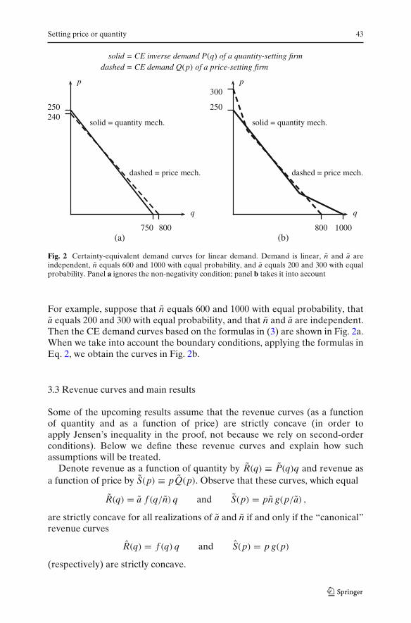
Example 1 Figure 2 illustrates the CE demand curves for linear demand,meaning that f (q) = 1 − q and g(p) = 1 − p. Over the range of quantities andprices for which the boundary of the linear demand curves are not reachedwith positive probability, we have the following CE demand curves:

P(q) = E[a] − qE[a/n] and Q(p) = E[n] − pE[n/a]. (3)


solid = CE inverse demand P(q) of a quantity-setting firmdashed = CE demand Q(p) of a price-setting firm

q

p

800750

250240

dashed = price mech.

solid = quantity mech.

q

p

800 1000

250

300

dashed = price mech.

solid = quantity mech.

(a) (b)

Fig. 2 Certainty-equivalent demand curves for linear demand. Demand is linear, n and a areindependent, n equals 600 and 1000 with equal probability, and a equals 200 and 300 with equalprobability. Panel a ignores the non-negativity condition; panel b takes it into account

For example, suppose that n equals 600 and 1000 with equal probability, thata equals 200 and 300 with equal probability, and that n and a are independent.Then the CE demand curves based on the formulas in (3) are shown in Fig. 2a.When we take into account the boundary conditions, applying the formulas inEq. 2, we obtain the curves in Fig. 2b.

3.3 Revenue curves and main results

Some of the upcoming results assume that the revenue curves (as a functionof quantity and as a function of price) are strictly concave (in order toapply Jensen’s inequality in the proof, not because we rely on second-orderconditions). Below we define these revenue curves and explain how suchassumptions will be treated.

Denote revenue as a function of quantity by R(q) ≡ P(q)q and revenue asa function of price by S(p) ≡ pQ(p). Observe that these curves, which equal

R(q) = a f (q/n) q and S(p) = pn g(p/a) ,

are strictly concave for all realizations of a and n if and only if the “canonical”revenue curves

R(q) = f (q) q and S(p) = p g(p)

(respectively) are strictly concave.


However, because R(q) and S(p) are positive, they could be strictly concaveon all of [0, ∞) only if they were strictly increasing. Therefore, we assumeinstead that R(q) is strictly concave on an interval [0, q] and that S(p) isstrictly concave on an interval [0, p]. Let nmin and amin be the greatest lowerbounds on the supports of n and a. Then R(q) is strictly concave on [0, nminq]for all realizations of demand and S(p) is strictly concave on [0, amin p] forall realizations of demand, respectively. We explore the significance of theseassumptions in Section 4.

3.3.1 Main results

Theorems 1 and 2 show that the increase in uncertainty about market sizecauses �∗

p − �∗q to rise, while the increase in uncertainty about valuations

causes �∗p − �∗

q to fall. More generally, by Theorem 1:

1. For a price-setting firm, the increase in uncertainty about market size hasno effect on the CE demand and therefore it has no effect on the profitfunction or on the maximum profit.

2. For a quantity-setting firm, the increase in uncertainty about market sizedampens the CE inverse demand and hence reduces the profit function andthe maximum profit—all under an assumption that the revenue function isstrictly concave on a large-enough domain (see Section 4).

Theorem 1 Suppose {n1, n2, a} are such that n2 is riskier than n1 given a.

1. For all p, Q(p; n2, a) = Q(p; n1, a) and hence �p(p; n2, a) = �p(p; n1, a).Therefore, �∗

p(n2, a) = �∗p(n1, a).

2. Suppose R(q) is strictly concave on [0, q]. For all q ∈ [0, nmin2 q],

P(q; n2, a) < P(q; n1, a) and hence �q(q; n2, a) < �q(q; n1, a). Therefore,if a solution to maxq �q(q; n2, a) lies in [0, nmin

2 q], then �∗q(n2, a) <

�∗q(n1, a).

By Theorem 2:

1. For a quantity-setting firm, the increase in uncertainty about valuations hasno effect on the CE inverse demand and therefore it has no effect on theprofit function or on the maximum profit.

2. For a price-setting firm, the increase in uncertainty about valuationsdampens the CE demand and hence reduces the profit function and themaximum profit—all under an assumption that the revenue function isstrictly concave on a large enough domain (see Section 4).

Theorem 2 Suppose {n; a1, a2} are such that a2 is riskier than a1 given n.

1. For all q, P(q; n, a2) = P(q; n, a1) and hence �q(q; n, a2) = �q(q; n, a1)

and �∗q(n, a2) = �∗

q(n, a1).


2. Suppose S(p) is strictly concave on [0, p]. Then, for all p ∈ [0, amin2 p],

Q(p; n, a2) < Q(p; n, a1) and hence �p(p; n, a2) < �p(p; n, a1). There-fore, if a solution to maxp �p(p; n, a2) lies in [0, amin

2 p], then �∗p(n, a2) <

�∗p(n, a1).

The proofs of these two theorems are identical except for a substitution ofthe roles of a and n, of f and g, et cetera. Therefore, the Appendix containsonly the proof of Theorem 1.

3.3.2 Remark on the standard additive-shock model

A standard representation of uncertain linear demand is Q(p) = α − βp,where β is known. The single parameter α scales both the horizontal andvertical intercepts; in our model, this means that n = α and a = α/β. Asa consequence, the CE inverse demand and demand curves are equivalent(assuming that p and q are such that formulas (1) do not result in negativevalues.) Therefore, this representation has the knife-edge property that theseller is indifferent between setting price and setting quantity no matter whatis the distribution of α.

This observation is interesting for two reasons. First, it means that the widelyused additive demand model (see e.g. Petruzzi and Dada 1999; Bhardwaj 2001;Chod and Rudi 2005) is very special. It also highlights that explicit modelingof the nature of demand uncertainty, which is the subject of our paper, isimportant. Second, it is also a benchmark that is useful for ranking the salesmechanisms. If we deviate from additive demand model by increasing theuncertainty about market size (valuations), then by Theorem 1 (Theorem 2)we know that setting price (quantity) is better than setting quantity (price).We summarize this conclusion in Proposition 1.

Proposition 1 Suppose that demand is linear.

1. If n = βa + x, where β > 0 and E[x | a] = 0 almost surely, then setting priceis better than setting quantity.

2. If a = n/β + x, where β > 0 and E[x | n] = 0 almost surely, then settingquantity is better than setting price.

4 Decreasing marginal revenue assumptions

The assumptions in Theorems 1 and 2, under which an increase in uncertaintyabout valuations (resp., market size) favors setting quantity (resp., settingprice), are that the revenue curves be concave on a large-enough domain.This section characterizes conditions under which the assumptions hold. Wedevelop the following ideas.

1. An empirical regularity is that demand becomes weakly more elastic athigher prices.


2. This implies that the “strict concavity of R” and “strict concavity of S”conditions hold on a range q ∈ [0, q] and p ∈ [0, p], respectively, thatincludes the optimal quantity and price as long as there is not too muchuncertainty and the marginal cost is low enough.

3. For the effect of market-size uncertainty on the expected profit of aquantity-setting firm, higher marginal cost merely strengthens the result(relaxes the condition on the amount of uncertainty).

4. In contrast, for the effect of valuation uncertainty on the expected profit ofa price-setting firm, higher marginal cost weakens the result (strengthensthe condition on the amount of uncertainty).

As noted, the property that demand becomes weakly more elastic at higherprices is an empirical regularity; we refer to it as “monotone elasticity”. Lineardemand has monotone elasticity as does the following variant of constant-elasticity demand: q = n(p−b − k), where b ∈ (0, 1) and k > 0. Given ourparametrization of demand uncertainty, a realization of the demand curve hasmonotone elasticity if and only if the canonical demand curves f and g havemonotone elasticity. Assume that this is true.

Consider first the canonical revenue curve R(q). Marginal revenue can bewritten as

R′(q) = p(

1 + 1

e

),

where p is the price f (q) when quantity is q and e is the elasticity at the point(q, p) on the demand curves. (Note that e is negative and we have assumedthat it becomes greater in magnitude for higher p and lower q.) One can usethis formula to show the following.

R1. R is maximized at the point qr at which e = −1.R2. R is strictly concave on an interval [0, q], where q > qr.R3. R is single peaked, meaning that it is decreasing for q > qr.

Likewise, consider the canonical revenue curve S(p). Marginal revenue canbe written

S′(p) = q (1 + e) .

One can use this formula to show the following.

S1. S is maximized at the point pr at which e = −1.S2. S is strictly concave on an interval [0, p], where p > pr.S3. S is single peaked, meaning that it is decreasing for p > pr.

Example 2 With linear demand, where f (q) = 1 − q and g(p) = 1 − p, therevenue curves are shown in Fig. 3. They are quadratic (and hence strictlyconcave) functions up until the intercepts, and hence we can take p = 1 andq = 1. The revenue maximizing values are qr = 1/2 and pr = 1/2.


q = 1qr = 1/ 2 q

R(q)

(a) Quantity-setting revenue

p = 1pr = 1/ 2 p

S(p)

(b) Price-setting revenue

Fig. 3 The canonical revenue curves for linear demand: f (q) = 1 − q and g(p) = 1 − p. aQuantity-setting revenue. b Price-setting revenue

Thus, over the domains [0, nmin] for quantities or [0, amin] for prices, theCE demand curves and the profit functions will shift as predicted by thesecond parts of Theorems 1 and 2. Theorem 1 is illustrated in Fig. 4, withindependent n and a. The dashed line assumes that n equals 700 or 900with equal probability; the solid line assumes that n equals 600 or 1000 withequal probability. As predicted by Theorem 1, the quantity-setting CE inversedemand curve, and hence the profit function, shift downward for q ∈ [0, 600].For high enough values of q, the shift is in the opposite direction.

Figure 5 illustrates Theorem 2, with independent n and a. The dashed lineassumes that a equals 240 or 260 with equal probability; the solid line assumesthat a equals 200 or 300 with equal probability. As predicted by Theorem 2, the

0 200 400 600 800q

p

250

P(q)

0 200 400 600 800

q

dashed = less risky n1

solid = more risky n2

nmin2 q

Πq(q)

Fig. 4 Illustration of Theorem 1 (effect of higher uncertainty about market size on quantity-settingCE inverse demand and profit function) for an example of linear demand; n and a are independent.Dashed curves are for less risky n1, equal to 700 or 900 with same probability. Solid curve is formore risky n2, equal to 600 or 1000 with same probability


0

50

100

150

200

250

300

q

p

800

Q(p)

0 50 100 150 200 250 300

dashed = less risky a1

solid = more risky a2

amin2 p

Πp(p)

Fig. 5 Illustration of Theorem 2 (effect of higher uncertainty about valuations on price-setting CEinverse demand and profit function) for an example of linear demand. n and a are independent.Dashed curves are for less risky a1, equal to 240 or 260 with same probability. Solid curve is formore risky a2, equal to 200 or 300 with same probability

price-setting CE demand curve shifts to the left, and hence the profit functionshifts downward, for p ∈ [0, 200]. For high enough values of p, the shift is inthe opposite direction.

Already R2 and S2 indicate that there are interesting domains on which thecomparisons of the profit functions in Theorems 1 and 2 hold. Next considerwhat it takes for these domains to be large enough for the comparisons ofmaximum profit to hold. We need to show that a solution to maxq �q(q; n2, a)

lies in [0, nmin2 q] and that a solution to maxp �p(p; n, a2) lies in [0, amin

2 p].Observe, for example, that this is true in Figs. 4 and 5.

Consider Theorem 2 and a quantity-setting firm. For any realization of theinverse demand curve f , revenue—and hence profit—is a decreasing functionof q on [nqr, ∞). Therefore, nmaxqr is an upper bound on the quantity that canmaximize expected profit. As long as nmax

2 qr < nmin2 q, that is, nmax

2 /nmin2 < q/qr,

we can conclude that the shift in the CE inverse demand curve causes themaximum expected profit to fall. If marginal cost is positive, we could weakenthe restriction because the profit-maximizing quantity would be lower andhence more likely to lie in [0, nmin

2 q].Consider Theorem 1 and a price-setting firm. Now we must be more

restrictive because the profit-maximizing price necessarily gets pushed up tothe region where the revenue curve is not concave as the marginal cost rises.Otherwise, however, the argument is similar. The condition amax

2 /amin2 < p/pr

guarantees that the price that maximizes expected revenue is in the strictlyconcave region of the revenue curve. As long as the marginal cost is smallenough, the profit-maximizing price is also in this region. We summarize thesetwo observations in Proposition 2.


Proposition 2

1. Suppose that {n1, n2, a} are such that n2 is riskier than n1 given a. Ifnmax

2 /nmin2 < q/qr then �∗

q(n2, a) < �∗(n1, a).2. Suppose that {n; a1, a2} are such that a2 is riskier than a1 given n. If

amax2 /amin

2 < p/pr then there is a c such that �∗p(n, a2) < �∗

p(n, a1) for c ∈[0, c].

On the other hand, consider linear demand with fixed {n, a1, a2}, where a2

is riskier than a1. Then for high-enough marginal cost the optimal price endsup where the CE demand curve for a2 is to the right of the one for a1, and thefirm is better off with the more uncertain valuations. The intuition is as follows.Suppose the marginal cost is high and therefore the firm sets a high price. It cando no worse than to have zero sales and this downside risk is not affected by anincrease in uncertainty about valuations. However, some times it will be luckyand sell at high price; this upside becomes more likely when there is greateruncertainty about valuations.

5 How the price-versus-quantity decision depends on the marginal cost

We now examine, for the case of linear demand, how the choice of salesmechanism depends on the magnitude of the marginal cost. We first ignorethe boundary constraint (i.e., we assume that the uncertainty about marketsize and valuations is not too large) and then show how the answer changeswhen we take it into account. As mentioned above, for any form of demand,marginal revenue cannot be decreasing everywhere (since revenue has to bepositive), and therefore the results of our analysis are rather general, and notjust an artifact of linear demand specification.

5.1 Analysis ignoring non-negativity constraints

Consider the example of the CE demand curves in Fig. 2a, which do not takeinto account the non-negativity constraints on quantity and price. Recall that(i) the choice of sales mechanism for a firm that faces uncertain demand isequivalent to (ii) the choice of CE demand curves for a firm with certaindemand but two demand curves from which to choose. A firm with decisionproblem (ii) would always choose a point on the outer (i.e., upper) envelope ofthe two demand curves. We can thus frame the choice of sales mechanism as:

1. choose a profit maximizing point on the outer envelope of the CE demandcurves P(q) and Q(p); then

2. see whether the solution comes from the P(q) curve or the Q(p) curve.

Figure 6a shows the outer envelope of the CE demand curves from Fig. 2a.The kink, where the outer envelope switches between P(q) and Q(p), ismarked with a dot. Because of the kink, the optimal price/quantity on this


solid = CE inverse demand P(q) of a quantity-setting firm

dashed = CE demand Q(p) of a price-setting firm

q

p

800

250

q

p

1000

300

(a) (b)

Fig. 6 Outer envelope of the CE demand curves for the example of linear demand in Fig. 2. Panela ignores the non-negativity condition, as in Fig. 2a; panel b takes into account the condition, as inFig. 2b

outer envelope does not vary continuously with marginal cost; in fact, it willjump over the kink as the marginal cost rises. Nevertheless, as a simple appli-cation of monotone comparative statics, we know that the optimal quantity isdecreasing and the optimal price is increasing as the cost rises because theobjective function π(q; c) = pq − cq has strictly decreasing differences in qand c. Therefore, as the marginal cost rises, the optimal price/quantity mayswitch from the dashed section (meaning that setting price is optimal) to thesolid section (meaning that setting quantity is optimal) but not vice versa.

To make sure that this conclusion is robust (as long as we ignore the non-negativity conditions) we just have to check that the CE curves can cross onlyas shown in Fig. 2a.

The formulas for the intercepts of the CE demand curves are shown inTable 1 for easy reference.

Proposition 3 Consider linear demand and ignore the non-negativity con-straints. Then either the CE demand curves do not cross or P(q) crosses Q(p)

from above, as illustrated in Fig. 2a.

Table 1 Intercepts of the CE inverse demand and demand curves for the linear case, ignoringnon-negativity constraints

Intercept P(q) Q(p)

Quantity E[a]/E[a/n] E[n]Price E[a] E[n]/E[n/a]


Proof We are ruling out the case in which the CE curves cross the other way,which would mean that the quantity intercept of Q(p) is lower than that ofP(q) whereas the price intercept of P(q) is lower than that of Q(p). FromTable 1, this translates into the following inequalities:

E[n] <E[a]

E[a/n] and E[a] <E[n]

E[n/a] . (4)

By multiplying the two inequalities together (LHS×LHS and RHS×RHS),then canceling E[n]E[a] from the resulting inequality, and then rearranging,we obtain E[a/n]E[n/a] < 1. This is impossible: for any nonnegative randomvariable z, E[z]E[1/z] ≥ 1. �

Proposition 3 leads to our main result on how the price-versus-quantitydecision depends on the magnitude of marginal cost.

Corollary 1 Suppose that demand is linear and consider the range of cost c suchthat the non-negativity constraints are not reached. If for some marginal cost c∗setting quantity is better for the seller, then it is better for any c > c∗. If for somemarginal cost c∗ setting price is better for the seller, then it is better for any c < c∗.

The result of Corollary 1 is, to some extent, counterintuitive. One wouldthink that if marginal cost is high, setting price is safer, since it will guaranteethat the product is never sold at a loss (i.e., below the marginal cost). However,this intuition is based on hitting the non-negativity constraint for quantity,as shown in the next subsection. The intuition for Corollary 1 comes fromProposition 3, showing the way the CE demand curves might cross.

5.2 Full analysis with non-negativity constraints

We now consider how the answer changes when we take into account the non-negativity constraints.

Consider the example of the CE demand curves in Fig. 2b. Figure 6b showstheir outer envelope. The kinks, where the outer envelope switches betweenP(q) and Q(p), are marked with a dot. As can be seen from Fig. 6b, the story ismore complicated than in Fig. 6a. If the CE curves cross three times, as in thispicture, then the optimal sales mechanism could switch from quantity to priceto quantity and then again to price as the marginal cost rises.

We can slightly simplify the possibilities by assuming that the bottom rightkink (crossing point) occurs at quantities beyond those that could maximizeprofit. This is true in the example because the quantity is greater than nmax/2,which bounds the optimal quantity. There are then three possible zones:

1. at low enough costs, the firm sets price;2. at an intermediate range of costs, the firm sets quantity;3. at an upper range of costs, the firm sets price.


Table 2 Intercepts of the CE inverse demand and demand curves for the linear case, taking intoaccount the non-negativity constraints

Intercept P(q) Q(p)

Quantity nmax E[n]Price E[a] amax

To ensure that these conclusions are robust, we must verify that the CEdemand curves cross as in Fig. 2b. In fact, this is true. Table 2 shows theintercepts of the CE curves. Along the vertical axis (low quantity, high price),the price-setting curve Q(p) must dominate. As long as the firm sets pricebelow amax, it gets some sales; in contrast, when setting quantity it can neverget an expected price that exceeds E[a]. By a similar argument, along thehorizontal axis (high quantity, low price) the quantity-setting curve P(q)

dominates. In fact, there are three possibilities.

1. The CE curves ignoring boundaries never cross because setting price dom-inates everywhere. Then the true CE curves cross only once, at low priceand high quantity, in a region that is never optimal even for zero marginalcost. Therefore, setting price is always optimal.

2. The CE curves ignoring boundaries never cross because setting quantitydominates everywhere. Then the true CE curves cross only once, at highprice and low quantity. If c = 0 then setting quantity is optimal; if c ≥ E[a]then setting price is optimal; in between, there is a single cost at which theoptimal mechanism switches from quantity to price.

3. The CE curves ignoring boundaries cross as illustrated in Fig. 2a. Then thetrue CE curves cross at this point and at two other points, one above andone below. If the optimal price/quantity at zero marginal cost is above themiddle crossing point, then this case ends up the same as case 1. Otherwise,at c = 0 and for c ≥ E[a], setting price is optimal. There may be a singleinterval of costs between 0 and E[a] for which setting quantity is optimal.

Results of this section (in particular, Corollary 1), where we have shownhow the price-versus-quantity decision depends on the marginal cost, arerelevant for manufacturer–retailer interactions. The retailer faces the problemwe have so far studied in this paper, but with its marginal cost equal to thewholesale price set by the manufacturer. Because of double marginalization,this wholesale price is greater than the marginal cost of the manufacturer. Asa consequence, the price-versus-quantity preferences of the retailer and themanufacturer might not be aligned. We study this issue in the following section.

6 Manufacturer–retailer interaction

We now consider a supply chain with an upstream manufacturer and a down-stream retailer, both risk neutral. The manufacturer has constant marginal costc. We restrict the manufacturer to a linear posted-price mechanism and denote


its price—which becomes the marginal cost of the retailer—by w. The retailer,on the other hand, can either set quantity or set price. We consider three cases.

1. The manufacturer can stipulate the mechanism used by the retailer (this ismeant to be a benchmark).

2. The retailer must commit to one of the two mechanisms before themanufacturer sets w.

3. The retailer selects its sales mechanism after the manufacturer sets w.

We assume that demand is linear and that the uncertainty is low enoughrelative to the cost that the boundaries of the linear demand curves are notrelevant. (The higher is the cost, the less uncertainty there can be aboutdemand so that the boundaries are avoided.) Thus, we use the formulas forlinear demand in Eq. 1, which do not take into account the non-negativityconditions. Alternatively, we rely on Section 5.1, and not on Section 5.2. Weuse subscript m (resp., r) to denote variables for the manufacturer (resp.,retailer).

6.1 Mechanism is selected before the wholesale price is set

Our analysis begins with the observation that the “certainty equivalent”approach extends to the supply chain if the mechanism is selected (by themanufacturer or retailer) in advance of the wholesale price w. That is, thequantity, price, and profit (or expectations thereof) for the parties are thesame as for a supply chain whose certain demand curve equals the mechanism’scertainty equivalent demand curve.

For example, suppose the retailer is committed to setting quantity. Let P(q)

be the CE inverse demand curve. Given w, the retailer chooses q to maximize(P(q) − w)q, just as it would if its inverse demand curve were known to beP(q). Let Qr(w) be the solution as a function of w. Then, whether demand iscertain or uncertain, the manufacturer chooses w to maximize (w − c)Qr(w).

Suppose instead the retailer is committed to setting price. Let Q(p) be theCE demand curve. Then the retailer chooses p to maximize (p − w)Q(p), justas it would if its demand curve were known to be Q(p). Let Qr(w) be theresulting expected sales as a function of w, which would equal its actual salesif its demand curve were certain. Either way, the manufacturer chooses w tomaximize (w − c)Qr(w).

Therefore, the choice of sales mechanism by the manufacturer or by theretailer is equivalent to the choice of CE demand curve P(q) or Q(p) in asupply chain with two possible demand curves. Our next step is to review theequilibrium profits for a supply chain with known demand.

The preceding observation does not depend on the assumption that demandis linear, but we now restrict attention to this case. Suppose, then, that theinverse demand and demand curves are known to be

p = a(1 − q/n) and q = n(1 − p/a).


One can show that the manufacturer sets w = (1/2)(a + c) (the midpointbetween the constant marginal cost c and the intercept a) and the retailer thensets p = (3/4)a + (1/4) (the midpoint between its constant marginal cost w andthe intercept a). The manufacturer’s price w is the same as the retail price ofthe coordinated channel. However, because the retailer’s price p is higher thanw, sales are half of what they would be in the coordinate channel. Therefore,the manufacturer’s profit is one half of the profit of the coordinated channel.In the supply chain, the manufacturer and retailer sell the same amount, butthe manufacturer’s markup is twice that of the retailers: (1/2)(a − c) versus(1/4)(a − c). Therefore, the manufacturer’s profit is twice that of the retailers.

With uncertainty and ignoring the boundaries, the CE inverse demand anddemand curves are linear. Applying the summary of the previous paragraph,we see that, for either sales mechanism, the retailer’s profit is half that of themanufacturer, which in turn is half that of the coordinated channel:

�∗q = 2�∗

qm = 4�∗qr and �∗

p = 2�∗pm = 4�∗

pr.

It follows that whichever CE demand curve (sales mechanism) gives thehighest profit to the coordinated channel also gives the highest profit to themanufacturer and to the retailer. It does not matter which party choosesthe sales mechanism — the decision would be the same. Furthermore, allour results from Sections 3–5 about how the nature of the uncertainty andthe marginal cost c affect the choice of sales mechanism for the coordinatedchannel apply to the choice of sales mechanism for the supply chain.

6.2 Retailer selects the mechanism after the wholesale price is set

Let M′ be the mechanism the manufacturer would select if it controlledthe choice, let w′ be the price the manufacturer would select given that themechanism is set to M′, and let �′

m be the resulting profit for the manufacturer.Here we suppose that the retailer selects the mechanism after w is set,

and consider whether the outcome for the manufacturer is still {M′, w′, �′m}

or it earns a lower profit than �′m because the retailer can choose the sales

mechanism after observing the wholesale price. We refer to parameters wherethe latter holds as a “conflict zone” because the manufacturer would preferto be able to force the mechanism M′ on the retailer and not allow for theretailer’s discretion.

Such a conflict occurs if, given w′, the retailer would not choose sales mech-anism M′. (We saw in Section 5 that the marginal cost influences the choice ofsales mechanism.) The manufacturer cannot achieve profit �′

m because either(a) it modifies w away from w′, so that the retailer chooses m′, or (b) the retaileruses a mechanism that yields a profit lower than �′

m for the manufacturer.Consider the CE curves shown in Fig. 2a and suppose that c = 0. For the

coordinated channel, the optimal price for either demand curve is one halfthe vertical intercept; we can see that the price-setting curve Q(p) dominates


in this region. Hence this is the mechanism that the manufacturer would liketo specify and that the retailer would also choose if it had to commit to amechanism in advance. Let w∗

p be the manufacturer’s optimal price if theretailer had to set price; w∗

p is one half the intercept of the dashed curve.Given w∗

p, the retailer would set a price halfway between w∗p and the vertical

intercept—in the region where the quantity-setting curve P(q) dominates.Therefore, the retailer prefers the quantity-setting mechanism.

Given our assumption that the boundaries of the demand curves are notrelevant, we know that an increase in marginal cost can cause a switch fromsetting price to setting quantity but not vice versa. Therefore, the only type ofconflict that can exist is as in the previous example: the manufacturer wouldprefer to commit to a price-setting mechanism but, given the manufacturer’swholesale price, the retailer would end up setting quantity.

This happens for an intermediate level of uncertainty about the valuationsof the consumers. With very little uncertainty about a, the CE demand curvesintersect near the vertical axis, and setting price will be optimal for both themanufacturer and for the retailer given w. With a lot of uncertainty about a,setting quantity dominates for the manufacturer and hence also for the retailer.

What does the manufacturer do in this conflict zone? It would not naivelyset w∗

p when it knows that the retailer would choose to set quantity. Thereare two possibilities: (a) the manufacturer may lower w to below w∗

p in orderto induce the retailer to set price; or (b) the manufacturer may accept that theretailer will set quantity and so chooses the price w∗

q > w∗p that is optimal given

that mechanism.Consider the following example. Let a and n be independent, with n equal

to 1 − δn and 1 + δn with equal probability and a equal to 1 − δa and 1 + δa withequal probability. Parameters δn and δa capture uncertainty about market sizeand valuations, respectively.

Fix c = 0 and δn = 0.1. Figure 7 plots wholesale price, manufacturer’s profit,and total channel profit as functions of δa under three possible scenarios:

1. the retailer sets price;2. the retailer sets quantity;3. the retailer chooses to set price or quantity.

In the range δa ≤ 0.05, the uncertainty about valuations is relatively lowand thus the manufacturer is better off when the retailer sets price, whichis also in the retailer’s interests. In the range δa > 0.1, the uncertainty aboutvaluations is large (compared to uncertainty about market size, δn = 0.1) andthus the manufacturer is better off when the retailer sets quantity; this is alsoin the retailer’s interests. Hence δa ≤ 0.05 and δa ≥ 0.1 correspond to “non-conflict” zones. In the range 0.05 < δa < 0.1, we observe the conflict zone: themanufacturer is better off if the retailer sets price, but the retailer prefersto set quantity when faced with the wholesale price w∗

p. For δa = 0.06 themanufacturer is better off by lowering the wholesale price to 0.47, so that theretailer then prefers to set price. For higher values of δa the manufacturer isbetter off letting the retailer to set quantity and thus setting the wholesale price


a)

0.465

0.47

0.475

0.48

0.485

0.49

0.495

0.5

0.505

0 0.05 0.1 0.15 0.2

retailer sets price

retailer sets quantity

retailer sets price or quantity

Wholesale Price

δa

b)

0.119

0.12

0.121

0.122

0.123

0.124

0.125

0.126

0 0.05 0.1 0.15 0.2

retailer sets price



δa

Manufacturer's Profit

c)

0.178

0.18

0.182

0.184

0.186

0.188

0.19

0.192

0.194

0.196

0 0.05 0.1 0.15 0.2

retailer sets price



δa

Channel Profit


� Fig. 7 Wholesale price a, manufacturer’s profit b, and total channel profit c as a function of δafor cases where the retailer sets price, the retailer sets quantity, and the retailer chooses betweensetting price or quantity

at w∗q. In other words, in the conflict zone the manufacturer must pay careful

attention to how its choice of wholesale price determines whether the retailersets price or quantity as its decision variable. Finally, observe that the totalchannel profit has a peak at δa = 0.06. The intuition is as follows: The lower isthe wholesale price, the better is channel coordination; since at that value ofδa the manufacturer is better off by lowering the wholesale price, total channelprofit goes up.

7 Conclusions

We examine how uncertainty about the demand curve influences a seller’schoice to set price or quantity. In particular, the seller could be uncertain aboutthe market size (e.g., the number of buyers) for its product or about how muchconsumers are willing to pay for the product. We show that greater uncertaintyabout market size favors setting price and greater uncertainty about valuationsfavors setting quantity. We also find a nonmonotonic relationship betweenmarginal cost and the choice of sales mechanism.

Framing the issues differently, we show that the seller needs to considerwhich of these two decision variables it should be more flexible on. Clearly,there are different costs to the seller of retaining flexibility of prices versusflexibility of quantity. Our analysis allows the seller to be informed on how thenature of uncertainty and the magnitude of marginal cost affect this trade-off.

We also consider the channel setting with a single manufacturer and a singleretailer. The interests of the manufacturer and retailer are aligned if there isprevailing uncertainty about either market size or about valuations. If bothuncertainties are comparable, then there exists a “conflict zone” in which themanufacturer prefers the retailer to set price but the retailer prefers to setquantity. In this situation the manufacturer must either (a) lower the wholesaleprice to the level at which the retailer prefers to set price or (b) let the retailerset quantity and adjust the wholesale price accordingly. The manufacturerwould then be better off if it could force the retailer to set the price.

The focus of our paper is on the effect of the nature of demand uncertaintyon the basic operation mode (to set price or to set quantity) preferred bya seller. We also show how the results extend to the channel setting. Weexpect that the effect of the uncertainty about different parameters of demandcurve on the seller’s choice of price versus quantity, illustrated in the simplemonopolistic one-shot sales model in this paper, will prevail under moresophisticated and realistic scenarios, such as auctions versus posted prices.

An interesting direction for future theoretic research could be the impact ofthe nature of demand uncertainty on other types of decisions, e.g., related to


inventory, either for a single seller or for the channel, possibly with competi-tion. On the empirical side, it would be important to distinguish and estimateuncertainty about market size and uncertainty about valuations.

Acknowledgements We thank Oleg Chuprinin and Kaifu Zhang for assistance, and the associateeditor and two anonymous referees for helpful and constructive comments.

Appendix: Proof of Theorem 1

Observe that

E[Q(p)

] = E[n g(p/a)] = E[E[n g(p/a) | a]] = E

[E[n | a] E[g(p/a)]], (5)

E[P(q)

] = E[a f (q/n)] = E[E[a f (q/n) | a]] = E

[a E[ f (q/n) | a]]. (6)

In each equation, the first equality is by substitution of the formulas for Q(p)

and P(q). The second equality is by iterative expectations. The third equalityfollows because we can treat a as a constant term when conditioning on it andhence move it out of the expectation.

Suppose that n2 is riskier than n1 given a. By definition, this means that theconditional distribution of n2 is riskier than the conditional distribution of n1,conditioning on a.

One implication is that E[n1 | a] = E[n2 | a] almost surely. Therefore, byEq. 5, E[Q(p; n1, a)] = E[Q(p; n2, a)]. This gives us part 1 of the theorem.

A second implication is that E[u(n2) | a] < E[u(n1) | a] almost surely for anystrictly concave u. In particular, suppose that

(a) n �→ f (q/n) is a strictly concave function of n on an interval that containsthe supports of n2 and n1.

Then E[ f (q/n2) | a] < E[ f (q/n1) | a] almost surely, and hence by Eq. 6 wehave E

[P(q; n2, a)

]< E

[P(q; n1, a)

]. To conclude the proof of part 2 of the

theorem, we need to show that (a) holds for q ∈ (0, nmin2 q] if

(b) R(q) is strictly concave on [0, q].Since n2 is riskier than n1 conditional on a, [nmin

2 , ∞) is an interval thatcontains the supports of n2 and n1. (Recall that nmin

2 is the greatest lower boundof the support of n2.)

For any function u(x) on R and any λ > 0, u is strictly concave on [z′, z′′]if and only if z �→ u(λz) is strictly concave on [z′/λ, z′′/λ]. Therefore, n �→f (q/n) is strictly concave on [nmin

2 , ∞) if and only if n �→ f (1/n) is strictlyconcave on [nmin

2 /q, ∞). The latter holds for all q ∈ (0, nmin2 q] if and only if it

holds for the largest such q, i.e., if and only if n �→ f (1/n) is strictly concave on[q, ∞).

The proof of Theorem 1 is then completed by using Lemma A.1. It says thatn �→ f (1/n) is strictly concave in n on [q, ∞) if and only if R(q) = f (q) q isstrictly concave in q on [0, q].


Lemma A.1 Let F : R+ → R+ be differentiable. Define G(x) ≡ xF(x) andH(y) ≡ F(1/y). Let y ∈ R++. Then H(y) is strictly concave on [y, ∞) if andonly if G is strictly concave on [0, 1/y].

Proof We provide a simple proof for differentiable F by showing that H′′(y) <

0 for all y ∈ [y, ∞) if and only if G′′(x) < 0 for all x ∈ [0, 1/y]. The lemmacan also be proved algebraically without differentiability; we omit the details.3

Observe that

G′(x) = xF ′(x) + F(x), H′(y) = − 1

y2F ′(1/y),

G′′(x) = xF ′′(x) + 2F ′(x), H′′(y) = 1

y4F ′′(1/y) + 2

y3F ′(1/y).

After canceling 1/y3 in the expression for H′′(y), H′′(y) < 0 is equivalent to

H(y) ≡ 1

yF ′′(1/y) + 2F ′(1/y) < 0.

By substituting x = 1/y, we see that H(y) < 0 for all y ≥ y if and only ifG′′(x) < 0 for all x ≤ 1/y. �

References

Bhardwaj, P. (2001). Delegating pricing decisions. Marketing Science, 20, 143–169.Budish, E., & Takeyama, L. (2001). Buy prices in online auctions: Irrationality on the internet?

Economic Letters, 72, 325–333.Caldentey, R., & Vulcano, G. (2007). Online auction and list price revenue management. Manage-

ment Science, 53(5), 795–813.Chod, J., & Rudi, N. (2005). Resource flexibility with responsive pricing. Operations Research,

53(3), 532–548.Etzion, H., Pinker, E., & Seidmann, A. (2006). Analyzing the simultaneous use of auctions and

posted prices for online selling. Manufacturing and Service Operations Management, 8(1), 68–91.

Fershtman, C., & Judd, K. L. (1987). Equilibrium incentives in oligopoly. American EconomicReview, 77, 927–940.

Hidvegi, Z., Wang, W., & Whinston, A. (2006). Buy-price english auctions. Journal of EconomicTheory, 129, 31–56.

Klemperer, P., & Meyer, M. (1986). Price competition versus quantity competition: The role ofuncertainty. Rand Journal of Economics, 17(4), 618–638.

Marvel, H. P., & Peck, J. (1995). Demand uncertainty and returns policies. International EconomicReview, 36(3), 691–714.

Matthews, T. (2004). The impact of discounting on an auction with a buyout option: A theoreticalanalysis motivated by ebays buy-it-now feature. Journal of Economics, 81(1), 25–52.

Miller, N., & Pazgal, A. (2001). The equivalence of price and quantity competition with delegation.RAND Journal of Economics, 32(2), 284–301.

Petruzzi, N., & Dada, M. (1999). Pricing and the newsvendor problem: A review with extensions.Operations Research, 47, 183–194.

3We thank Oleg Chuprinin and Kaifu Zhang for providing us with the algebraic proof.


Rothschild, M., & Stiglitz, J. (1970). Increasing risk: I. A definition. Journal of Economic Theory,2, 225–243.

Sklivas, S. D. (1987). The strategic choice of managerial incentives. RAND Journal of Economics,18, 452–458.

Vives, X. (1999). Oligopoly pricing. Cambridge: MIT.Wang, R. (1993). Auctions versus posted-price selling. American Economic Review, 83(4), 838–

851.Wang, X., Montgomery, A. L., & Srinivasan, K. (2008). When auction meets fixed price: A

theoretical and empirical examination of buy-it-now auctions. Quantitative Marketing andEconomics, 6(4), 339–70.

Weitzman, M. L. (1974). Prices vs. quantities. The Review of Economic Studies, 41(4), 477–491.

setting price or quantity: depends on what the seller is more

Documents