setting the boundary conditions ansys cfx -...
TRANSCRIPT
1
Ahmed Al Makky
Setting Up
the Boundary
Conditions
ANSYS CFX

2
@Ahmed Al Makky 2018
All rights reserved. No part of this publication may be reproduced, stored in a retrieval system or
transmitted in any form or by any means, electronic, mechanical or photo-copying, recording, or
otherwise without the prior permission of the publisher.
3
Tutorial 2:
Setting the boundary conditions on the studied
model using ANSYS
Introduction:
This tutorial is a continuation from the previous tutorial, we will be assigning the boundary conditions
to the studied domain such as inflow, out flow and etc …. .
Why is it that we need to specify the boundary condition?
During this tutorial a simple geometry is used, the objective of that is that the student masters the
steps to get to run a simple simulation, once that’s done the student can model any kind of geometry
he sees necessary for his studied case.
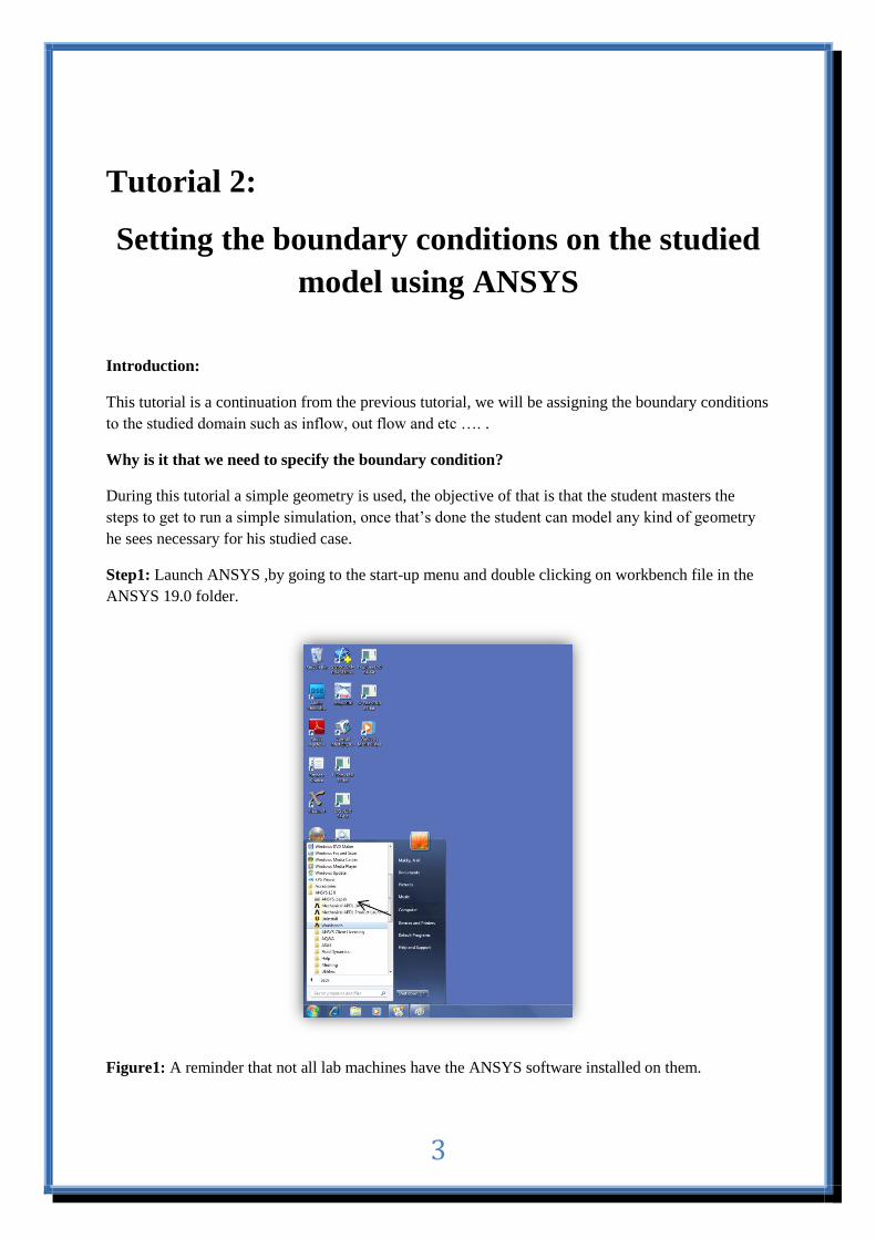
Step1: Launch ANSYS ,by going to the start-up menu and double clicking on workbench file in the
ANSYS 19.0 folder.
Figure1: A reminder that not all lab machines have the ANSYS software installed on them.

4
Step2: Once the program is launched it should look like as shown below. Go to Analysis Systems
(CFX) and double click.
Figure2: You might have to wait a bit till ANSYS gets running, the student is encouraged to use the
provided help with the software, it has lots of useful hints here and there.

5
Step3: Next Double click on the Geometry. This stage is for getting the required geometry read into
the software, note that there is a blue question mark icon beside the geometry text. Looking at the
bottom of the window you will see two windows one having the title of Messages, this title confirms
that the imported geometry has no problems with it, the next window has the title Progress and that is
necessary to prove that state of the progress and if there is a problem it will state the problem.
Figure3: At the moment the illustration are a bit simplified for the user and will get complex with
time.
Step4: Once ANSYS Workbench window is active you will get a window asking to specify working
units for the model dimension chose meters and press ok. For the user this step might seem secondary
in importance but as a matter of fact it’s of great importance, because at later stages you will have to
specify the box size (discrete element dimension). Box size dimension leads to finer mesh, the finer
the used mesh is the more accurate is the captured data. The captured data term refers to the fluid flow
structures.

6
Figure4: Depending on your studied case the selection of serial or parallel is taken, also depending on
the hardware provided in the computer lab dual core or quad core etc.
Step5: Go to file and choose Import External Geometry File…. .
Figure 5:.
7
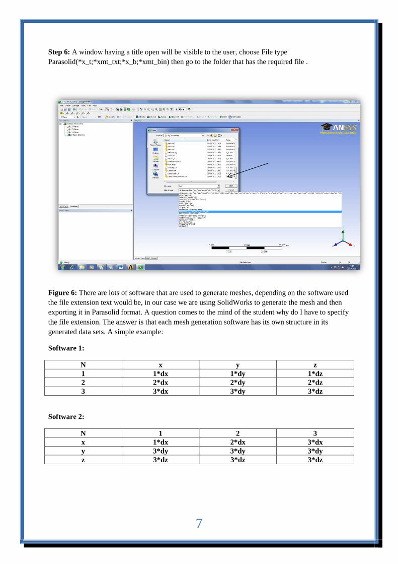
Step 6: A window having a title open will be visible to the user, choose File type
Parasolid(*x_t;*xmt_txt;*x_b;*xmt_bin) then go to the folder that has the required file .
Figure 6: There are lots of software that are used to generate meshes, depending on the software used
the file extension text would be, in our case we are using SolidWorks to generate the mesh and then
exporting it in Parasolid format. A question comes to the mind of the student why do I have to specify
the file extension. The answer is that each mesh generation software has its own structure in its
generated data sets. A simple example:
Software 1:
N x y z
1 1*dx 1*dy 1*dz
2 2*dx 2*dy 2*dz
3 3*dx 3*dy 3*dz
Software 2:
N 1 2 3
x 1*dx 2*dx 3*dx
y 3*dy 3*dy 3*dy
z 3*dz 3*dz 3*dz

8
Step7: Looking at the DesigModeler window, we can’t see the imported geometry yet, what is
required next is to press on the generate icon that is represented by a yellow thunder icon.
Figure6: The DesignModeler will read in the imported data file, and will construct the required mesh.
Step7: The imported Geometry Domain should look something like this, still that doesn’t give any
hints to the user, relating to the inner structure of the domain.
Figure7: The geometry domain is viewed in the shaded exterior style.
9
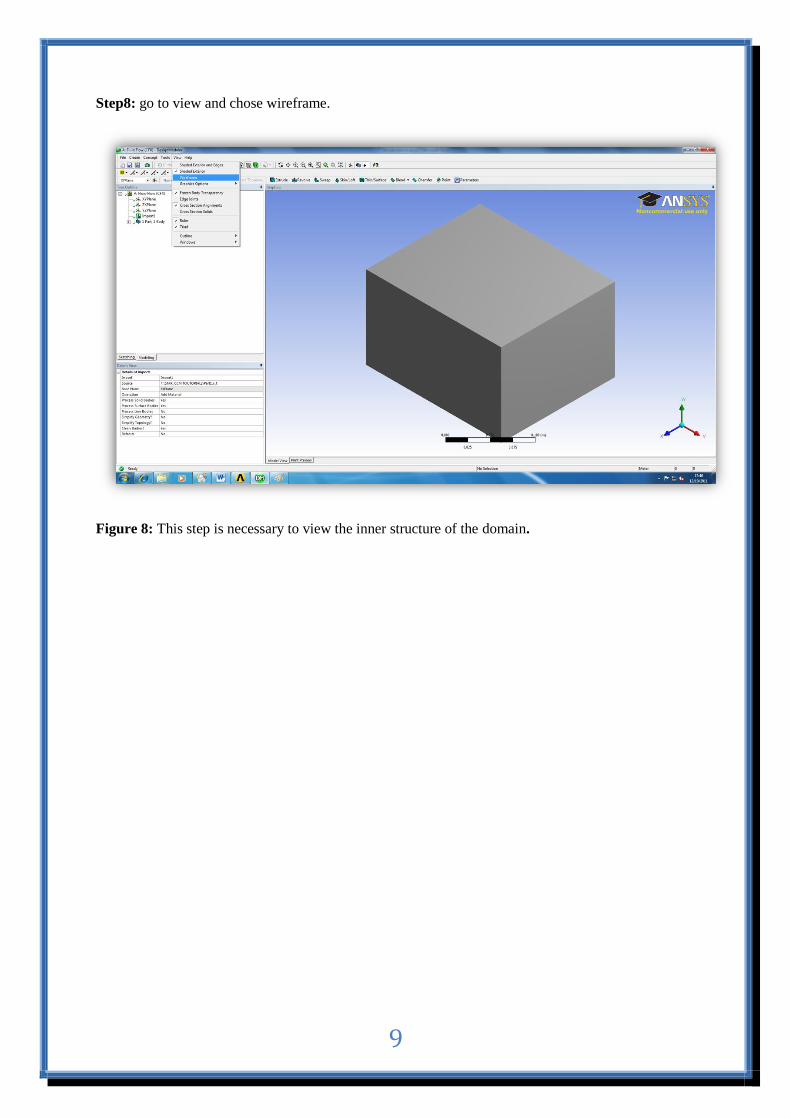
Step8: go to view and chose wireframe.
Figure 8: This step is necessary to view the inner structure of the domain.

10
On screen element selection (Left
Button):
Press once on the specified
element to study.
Rotation of View (Middle Button):
Press once on the specified point
on the screen and move mouse
you can rotate your view angle.
Zoom of View (Right Button):
Press once and the specified
point on the screen and move
mouse you zoom your view
angle.
11
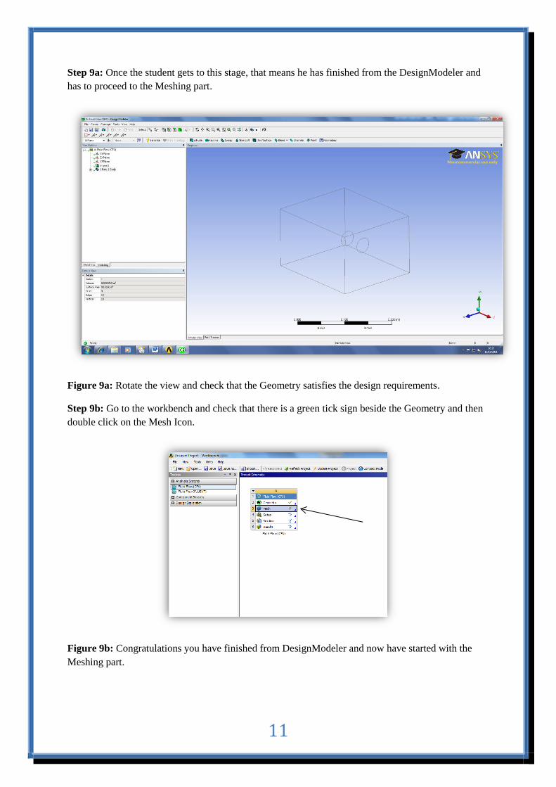
Step 9a: Once the student gets to this stage, that means he has finished from the DesignModeler and
has to proceed to the Meshing part.
Figure 9a: Rotate the view and check that the Geometry satisfies the design requirements.
Step 9b: Go to the workbench and check that there is a green tick sign beside the Geometry and then
double click on the Mesh Icon.
Figure 9b: Congratulations you have finished from DesignModeler and now have started with the
Meshing part.

12
Step 10a: The Meshing part of the project has started, notice that beside the Mesh there is a yellow
thunder icon.
Figure 10a: The scale shown at the bottom helps you make the right decision on the box sizeing, so
that we can see that the largest value on the scale is 0.200(m) which means we have to chose a value
less than 0.050(m).
Step 10b: right click on Mesh and chose Insert and then chose Method.
Figure 10b: at this stage we come to the point where we have to choose what kind of mesh are we
going to use wither regular or irregular or etc.

13
Step 10c: click on the positive sign beside the Mesh you should get a tree subbranch have
automatic Method using the left button click on the grey box domain, as a result it should by
highlighted in green, then you see that the geometry text is highlighted in blue press the apply.
Figure 10c: choose the parallel option in the projection mode, which will come handy later on, when
you want to use the measure command or choosing the appropriate slice plane for your study.
Step 11: go to method and choose Tetrahedrons.
Figure 11: This prepares the view for later wanted operations.

14
Step 12: Go to algorithms and choose Patch Independent.
Figure12: Now that you have specified the mesh properties, you can proceed to the next step .
Step13: press the Update icon and then press on the Generate Mesh icon.
Figure13: For our case we will want to now the dimensions of the inflow section of the pipe.

15
Step14: click on mesh, now it’s visible to the user the generated mesh.
Figure 14: Click on the middle button to rotate the view to inspect your mesh.
Step15: Go to work bench, you will see there is a green tick beside the mesh congratulations .
Figure15: Looking at the Output-star 1 you will see the coordinates of the points that you selected.

16
Step16: Changing the transparency of the mesh is essential to identify if there are any defects in the
internal structure of the studied mesh.
Figure16: The transparency icon is shown by an icon that has different plans with different colours in
a Cartesian coordinate’s system space.
Step17: Try using the rotate, pan or zoom view to get a view that looks something like this.
Figure17: Once you’re happy with it processed to the next step.
17
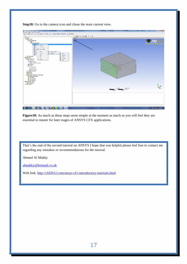
Step18: Go to the camera icon and chose the store current view.
Figure18: As much as these steps seem simple at the moment as much as you will feel they are
essential to master for later stages of ANSYS CFX applications.
That’s the end of the second tutorial on ANSYS I hope that was helpful please feel free to contact me
regarding any mistakes or recommendations for the tutorial.
Ahmed Al Makky
Web link: http://cfd2012.com/ansys-cfx-introductory-tutorials.html