setting up a mixed reality simulator for using … · setting up a mixed reality simulator for ......

F. López Peña, et al., Int. J. Sus. Dev. Plann. Vol. 11, No. 4 (2016) 616–626

© 2016 Fernando López Peña, Pilar Caamaño, Gervasio Varela, Félix Orjales, & Alvaro Deibe. May be used for research, academic, policy or other non-commercial purposes but with a citation to this source.ISSN: 1743-7601 (paper format), ISSN: 1743-761X (online), http://www.witpress.com/journalsDOI: 10.2495/SDP-V11-N4-616-626

This paper is part of the Proceedings of the 24th International Conference on Modelling, Monitoring and Management of Air Pollution (Air Pollution 2016) www.witconferences.com

SETTING UP A MIXED REALITY SIMULATOR FOR USING TEAMS OF AUTONOMOUS UAVS IN

AIR POLLUTION MONITORING

F. LÓPEZ PEÑA1, P. CAAMAÑO2, G. VARELA3, F. ORJALES1 & A. DEIBE1

1Integrated Group for Engineering Research, Universidade da Coruña, Spain. 2NATO Centre for Maritime Research and Experimentation, Italy.

3Mytech Ingeniería Aplicada S.L., Spain.

ABSTRACTA framework based on a mixed reality simulator for coordinating teams of autonomous Unmanned Aerial Vehicles (UAVs) is been developed. This framework would serve as a tool to facilitate crossing the reality gap for different applications; particularly when using these UAVs teams for air pollution monitoring and measurement. The system is built on a co-evolutionary simulator that makes use of data transmitted from some real UAVs to integrate them within a team of simulated UAVs. The system allows the progressive increase of the number of real UAV in the team. This facilitates the setting-up of a single UAV control system and also of the UAV collaboration schemes for different scenarios. A specific implementation of this system focussed on mapping the pollutant dispersion of a plume in the atmosphere is presented. Implementing an appropriate pollution dispersion model within the simu-lator is a key aspect of the system. This model should require few computational resources, should be easy to adapt in real time to ambient changes, and it should have a fair accuracy.Keywords: mixed reality, plume dispersion, unmanned aerial vehicles.

1 INTRODUCTIONA mixed reality simulator aiming to coordinating teams of autonomous Unmanned Aerial Vehicles (UAVs) is been developed as a framework to facilitate crossing the so-called reality gap. The ‘reality gap’ term has been coined at the end of the last century pointing to the fact that often robot controllers evolved in simulation result to be inefficient once the system is transferred onto the real world, as in Jakobi et al. [1] or in Nolfi and Floreano [2]. Furthermore, when seeking multi-robot collaboration strategies, as in the case of collective UAV systems, the problem is compounded and the reality gap arising from collective behaviour issues should be added to the inherent reality gap of each individual.

This paper presents the setting-up and first use of this simulator when applied to air pollu-tion dispersion monitoring. This simulator framework makes use of the telemetry and data transmitted from some real UAVs to integrate them within a team of simulated UAVs. The data measured by the sensors of the real UAVs are used as ground truth to adjust the param-eters of the world model used within the simulator. The system is designed to allow progressively increasing the number of real UAVs in the team. Thus, starting with just one real UAV it would be possible to check its controller, its behaviour, the communications and all the other physical aspects that could introduce discrepancies when moving to the real world. Then, adding more UAVs would allow verifying and adjusting the coordination and collaborative functions of the team. This progressive procedure facilitates the setting-up of the mission while minimizing risks and costs.

F. López Peña, et al., Int. J. Sus. Dev. Plann. Vol. 11, No. 4 (2016) 617

The simulation environment is an evolution of the one presented by Varela et al. [3]. It is conceived as a distributed multi-agent system where the planes are autonomous agents flying either in a real or a virtual world. It is built in such a way that the mission controlling algo-rithms are completely decoupled from the flight dynamics of the planes. This allows the use of combinations of different kinds of simulated and/or real planes. The simulation environ-ment uses a central control point, called Squadron Controller (SC) that uses the Google Maps API for monitoring and visualization purposes and for global squadron control. The SC com-municates remotely, via UDP/IP, with a Virtual Aircraft (VA) application that can be run in remote computers, so that a computation cluster can be used to run multiple planes. This remote operation capability allows running a VA directly in the flight field, connected via an RF data link to the real plane and remotely connected to the SC via Internet.

2 THE SIMULATOR FRAMEWORKThe design of the simulator framework should allow the simultaneous execution of coordinated teams of UAVs composed by arbitrary numbers of simulated and real UAVs. In addition, it should also allow to feed the simulator with real data, both off-line or on-line (i.e. at real time) to adjust the behaviour of the different simulated elements, so that they get closer to reality.

With these requirements in mind, we have designed the simulator as a distributed multi-agent system, where each element is an agent that can be run on different computers located in different physical places. Furthermore, each element provides their own entry points for data coming from the real world to allow adjusting their behaviour to the conditions and constraints of the reality. The proposed framework is divided into three main elements or types of agents: the SC, the world simulator (WS), and the VA. All the different elements can be distributed, and they communicate between them using a custom UDP/IP binary protocol.

The VAs represent the different UAVs deployed in the system, with one VA agent for each simulated or real UAV. All the VAs, regardless of their type, are equal inside the simulator, so it is transparent for the developers to deploy the system with zero, one or N physical UAVs. Any VA has two different components; the Airplane Closed Loop and the Autopilot. The Airplane Closed Loop is where the autonomous behaviour of the VA resides; it is in charge of deciding which action to do next. For the setting-up presented in this paper, the VA only receives setpoints from the SC. Then the Autopilot module controls the flight of the UAV by translating these setpoints into flight instructions.

The SC acts as a ground station for controlling, monitoring and visualization purposes. It has two main goals; first of all, it is in charge of automatically communicating with both, the environment simulator and the VAs to receive status information. When this information comes from real VAs, the SC uses it to feed the WS with real data, so that the simulation of the world can be improved. In addition, the SC can implement some parts of the behaviour of the coordination strategy. The SC includes also some monitoring tools, like a map visualiza-tion tool by using Google Maps and logging utilities.

The main purpose of the simulator third block, the WS, is to provide the SC and the VAs with information about the situation of the mixed-reality world where the VAs operate. It has two main purposes. On one hand, it must simulate the real outdoor environment. Furthermore, the WS is connected to each instance of the simulated VAs, and feeds them with ambient data coming from the real UAVs. On the other hand, the WS must simulate the sensors, emitting sources and pollution dispersion characterizing the problem to be assessed. Real aircraft could also send their actual sensor information via the SC to continuously adapt and correct the embedded pollutant dispersion models.

618 F. López Peña, et al., Int. J. Sus. Dev. Plann. Vol. 11, No. 4 (2016)

3 UAVS DESCRIPTION

3.1 Real UAVs

The UAVs selected for this case are flying wings, with all of their components embedded in the wing. The wings are made of EPP foam (Expanded Polypropylene). Figure 1 presents a picture of some UAVs currently used for testing.

There are three RF communication paths between each plane and its associated ground equipment. The first one is the Radio Control Link; it lets a human pilot control the plane from a standard RC transmitter. For safety reasons, this control by a human can be taken at any time. The second communication path is the Video Link and the third one is the data link.

The Video Link serves two purposes. On one hand, it is used to download real-time ana-logue video from the on-board camera. On the camera image, it is superimposed exhaustive information from the on-board electronics, such as GPS data, barometric altitude, pilot speed, geographic plane location, etc. This can help the pilot to control the plane in first person view in the event of an out of sight situation. On the other hand, the on-board electronics embed all available collected data in the Teletext space of the video link, in such a way that the ground equipment can extract and use this information in real time.

The third communication path is the data link. It duplicates the data download of the video link, for security reasons and, at the same time, it serves as the primary source of communica-tion for the automated UAV operations.

3.2 Virtual UAVs

The virtual UAVs allow the developers of the coordination strategy to easily test their imple-mentation at the lab. At first, only simulated UAVs are used, and then progressively real UAVs are added to the tests to validate the strategy and to introduce real data into the simula-tor to reduce the reality gap.

The simulated UAVs fly in a synthetic environment based on the open source FlightGear flight simulator [4]. Each simulated plane operates in an independent instance of FlighGear,

Figure 1: Some UAVs used for testing.


and all of them communicate with each other, and with the SC. As it has been said, this allows spreading the computational effort over different machines. The flight dynamics of each sim-ulated UAV are modelled with jsbsim, an open source Flight Dynamics Model (FDM). A jsbsim airplane model has been programmed and specifically tuned to match the physical characteristics of the real UAVs.

The geographic model of FlightGear is based on orthoimages, and the elevation data are obtained from Shuttle Radar Topography Mission (SRTM). Real-time weather is also simu-lated in FlightGear, helping to close the reality gap between virtual and real environment.

3.3 Control

In the real UAVs three modes of control have been implemented having different safety lev-els. The first mode is an automated control based on algorithms running onboard and aiming to control the airplane when flying in a standard automated manner. It drives the UAV follow-ing setpoints uploaded from the SC and using data from the onboard sensors such as GPS, barometric sensor, or Pitot tube. The ground station unit communicates with the airborne planes and links them to the remote SC and the rest of (virtual) planes of the swarm.

A human pilot can take control of the plane at all times, using the RC link and an RC trans-mitter for each plane. Video and audio links, with embedded sensor and status information help the pilot to control the plane in first person view in the event of an out of sight situation, as has been said.

Dedicated electronics watch for the radio links integrity, and transfer the plane control to the third, lower level, controller if need be. This stage – the Guardian Controller – is based on a commercial unit that uses GPS, IMU, Pitot and barometric sensors to control the plane, and is able to return it automatically to the takeoff point, in case of a total link loss.

With the aim of making the simulated UAVs behaviour as close as possible to reality, the control strategy is divided into four blocks as shown in Fig. 2. The only difference between real and simulated UAVs is the source of the data needed to determine the values of the

Figure 2: UAV control strategy.


variables. In the real ones this is coming from the onboard sensors while in the simulated ones come from the simulator.

Two of the blocks in Fig. 2 form an Inner Loop, controlling airspeed and roll. These blocks use roll and airspeed variables, and control the elevator and aileron of the plane. With this inner loop correctly tuned, the plane flies by itself with a constant attitude. In the real planes this loop is the Guardian itself.

The Outer Loop controls implement a Total Energy Compensation controller and a head-ing control. With this loop tuned, the SC or the human pilot can control the course, speed and altitude of the plane. This higher abstraction control layer is exactly the same in both the real and simulated planes.

4 SETTING UP THE MIXED-REALITY FRAMEWORKThe proposed simulator framework could be used for many scenarios and applications. Thus, it is necessary to set it up by taking into account the specific characteristics of the current application. In the present case it will make use the Google Maps API to represent the geo-graphic region under analysis. In addition, it includes a model for the particular pollutant dispersion case. In the following sub-section we describe how to set up the simulator for this purpose.

4.1 Plume modelling

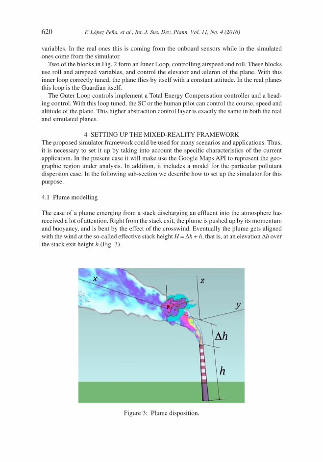
The case of a plume emerging from a stack discharging an effluent into the atmosphere has received a lot of attention. Right from the stack exit, the plume is pushed up by its momentum and buoyancy, and is bent by the effect of the crosswind. Eventually the plume gets aligned with the wind at the so-called effective stack height H = Dh + h, that is, at an elevation Dh over the stack exit height h (Fig. 3).

Figure 3: Plume disposition.


Selecting an adequate pollutant dispersion model is of paramount importance of having a virtual world able to correctly represent the relevant features of the real world. In this sense, selecting a highly accurate model could appear to be an adequate choice. However, the model also needs to be computationally light and easily configurable. This way it will facilitate its implementation making possible to adapt it in real time to the changing conditions in the real world. For these reasons, we have resorted on parametric plume dispersion models instead of going to more sophisticated ones.

The Gaussian plume models determine that, once the plume has been completely developed and for a given position along the x-axis, the pollutant dissemination along y and z axes follows a Gaussian distribution. Then the whole plume dispersion process is governed by fewer param-eters, as the mass flow of pollutant exiting the stack Q. The Gaussian model for the plume expresses the distribution of pollutant concentration c in the flow field within the plume as:

c x y zQ

u

y z

y z y z

( , , ) exp exp= − −

2 2 2

2

2

2

2p s s s s (1)

Where σy and σz are the Gaussian standard deviations along the y and z-axes at a given x posi-tion, and u is the wind speed.

There can be found in the literature different ways for obtaining σy and σz. The semi empirical formulation of Briggs [5] is generally accepted and is the one that is used in the present work. These Briggs sigma functions depend on the atmosphere stability classes, named from A to F, established by Pasquill [6]. The Brigss’ estimations of these standard deviations could be corrected during each test in view of the data obtained by the real UAVs.

A plume rise model aiming to estimate the elevation Dh uses to be included as a part or complement of any Gaussian plume model. However, the framework presented here doesn’t need to use any of these rise models as the elevation Dh can be directly measured by the UAVs during some preliminary flights for each test session. During these flights, the maxi-mum level of pollutant concentration is measured at several distances x from the stack. From expression (1) the maximum concentration at a given position x can be expressed as:

c xQ

uMAX

y z

( ) =2p s s

(2)

The preliminary tests flights serve to measure this cMAX. The position where the UAV is measuring this maximum concentration determines also the effective stack height H and serves to adjust the actual position of the x-axis.

As in many cases the mass flow of pollutant exiting the stack Q is not known, it results of interest to write the pollutant concentration distribution (1) in function of cMAX:

c x y z cy z

MAXy z

( , , ) exp exp= − −

2

2

2

22 2s s

(3)

With this formulation, the only parameters of the Gaussian model that are at first estimated are the Gaussian standard deviations σy and σz.

4.2 Setting up the squadron controller

The SC is in charge of implementing the behaviour of the UAVs coordination strategy. The SC receives the information that comes from the two types of VAs (real or virtual) and uses


it to drive the flight of the group of VAs over the environment. It does so by analyzing the received information to generate a group of setpoints that, depending on the problem to be solved, represent promising solutions. In the present case, these promising points represent interesting positions on the environment in terms of pollution concentration.

In this work, the Constrained Sampling Evolutionary Algorithm (CS-EA) has been used as part of the operation of the SC. The CS-EA is an evolutionary algorithm (EA) variant previously developed by the authors as it is explained in detail in [7]. This variant is based on the common cycle of a standard EA but taking into account the limitations imposed by the application where it is not possible to directly move the UAVs, which are sensing the environment to produce the fitness value of the EA, to the positions of the search space proposed by the EA.

The setting-up of the CS-EA requires the specification of the EA that is going to be used as which is called basis-EA. In this work, a Differential Evolution algorithm (DE) [8] has been used. The parameterization of the DE has been done using the values recommended in [9]. That is, the differential weight parameter (F) has been set to 0.9, the crossover rate (CR) has been set to 0.1, while the population size has been set to 100 individuals.

With this parameter configuration, the CS-EA will provide a population of 100 promising positions of the search space. At this point it is necessary to assign one of these positions to each VA of the squadron. Evidently, it is not practical and approachable to use one VA, real or simulated, for each individual of the population. Thus, as the number of VAs will be lower than the population size, it is necessary to establish a strategy to select a promising point for each VA with which drives its flight. In this work, due to physical constraints of the VAs and with the aim of avoiding sudden manoeuvres that although could be possible in simulated VAs are not realistic when dealing with real VAs, the strategy implemented selects a random promising point within a range from the VA position. In our experiments, an angle of 45 degrees charac-terizes this range.

5 TESTINGThis section presents some results obtained during the tests performed using a real UAV coordinated with a team of simulated UAVs having the mission of finding and characterizing a source of an atmospheric pollutant. The source under analysis for this test bench is a plume exhausted from the Thermal Power Plant (TPP) of As Pontes that is located in the region of Galicia, Spain. As Pontes TPP has four coal-fired independent power generation units of 350 MW each and it has a 356 m above ground level (AGL) exhaust stack. In this case, CO2 is the greenhouse gas used for monitoring and mapping.

The first step for each test session concerns the adjustments of the flight controls and the sensors of the real and simulated UAVs. A conventional and common application of mixed reality is for adjusting and setting-up the flight controls of UAVs. This is a customary and necessary preliminary step when using UAVs for sensing.

The second step is to adjust the parameters for the environment and the mission models that are implemented in the simulator. In the present case the environment corresponds to an outdoor flight for which wind speed and direction is very important. In addition, the initial values of H and cMAX need to be determined. Thus, some specific flights have been performed to adjust these parameters.

The last step concerns the adjustment of the coordination algorithm acting behind the SC. As in the previous case, this algorithm needs to be adjusted and validated. In this case, we have resorted on an incremental adjustment of this algorithm as a mean of progressively reduce the reality gap.


5.1 Adjusting the flight controls

The first and obvious use of the simulator is for adjusting the flight controllers of the UAVs. As it has been said in the previous sections, the control strategy of the UAVs is split into an inner and an outer loop.

The controllers of real and simulated UAVs are based on typical PID controllers. The pro-portional, integral and derivative terms of each controller need to be adjusted to the dynamic behaviour of the planes. To fine tune these parameters an incremental approach was taken. In the first place, the virtual environment of FlightGear and Jsbsim were used to simulate the dynamics of the plane in different weather situations. A Java based script allows to implement the controllers and to tune their parameters. The script also generated UAV flight data that have been used in the tuning process.

All the control parameters of the real UAVs were initially set matching the values obtained for their pairs in the virtual environment tuning process. After that, some specific flights were made to fine tune these parameters in the real environment. First, the inner loop controllers and then the outer loop ones. The parameters obtained in this real environment tests were used onwards on both real and simulated plane controllers, thus making the behaviour of real and simulated planes as close as possible, and closing the reality gap.

Some CO2 measurements have been obtained in these flight tests as well. This data was used to calibrate and fine tune the behaviour of the CO2 sensors, as well as establishing base CO2 levels (blue colour in the flight path).

5.2 Adjusting the environment and plume model parameters

Some tests have been performed where a single real UAV has been coordinated with a team of simulated UAVs. The mission has been that of finding and characterizing a source of an atmospheric pollutant starting from the stack output of the “As Pontes” TPP. Following the strategy presented earlier, the information obtained from the real UAV has been used to adjust the values of the parameters governing the Gaussian plume pollutant dispersion model. To illustrate the importance of this action, Fig. 4 presents one of the real UAV test flights. The figure represents by means of a colour coding the values of the CO2 concentration measured by the UAV sensor on the flight path. These concentration values have been recorded together with the GPS data in a KML file and then represented on Google Earth. The coded colours range from grey to red. Grey corresponds to a concentration of 450 ppm or less, and red cor-responds to 840 ppm or more. The measured base concentration level in the free air was of 449 ppm. The maximum CO2 concentration measured at a distance of 2.4 Km from the stack was of 859 ppm. This maximum concentration was measured at an effective stack height of 486 m. Therefore, the origin of coordinates has been placed in the simulator at this level on the vertical of the stack. The x-axis is taken as the line defined by the origin and the position where cMAX is measured.

5.3 Incremental adjustment of the coordination algorithm

From the SC point of view, that is to say that the features of the search space are continually modified during the search or characterization process. This is one of the reasons that support the choice of an EA-based approach, as this type of algorithms had shown a great perfor-mance in the resolution of problems in which the search space is dynamically modified.


As shown in [9], the EA works by generating, step-by-step, new populations of promising points where the maximum value of CO2 would be read. Each plane uses a strategy to select one of those points, and it tries to reach that point until a new step from the EA algorithm selects a new set of promising points. The planes are continuously feeding the EA with new data from the field, with is used by the EA in each step to generate a new population of chil-dren points more promising than the previous one.

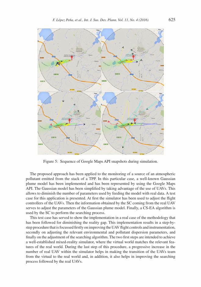
The test carried out within this work has been performed by using five simulated UAVs and one real UAV. In each snapshot of Fig. 5, the UAVs are represented by arrows; the black ones are for the simulated UAVs and the red ones for the real UAVs. The trajectory followed by each one is also represented by using colour lines. During their flight, both types of UAVs are sensing the environment, this information is used to feed the CS-EA. The set of promising point proposed by the CS-EA are represented by yellow starts.

As it is shown in the sequence of snapshots, as the execution progresses and more informa-tion from the environment is available, the EA population is getting closer to the point of maximum concentration of the plume.

6 CONCLUSIONSA framework for developing coordinated teams of autonomous UAVs based on a mixed-reality simulator making use of real and simulated UAVs is presented. The simulator is a distributed multi-agent system where both real and simulated UAVs are autonomous agents. This architecture allows the progressive increase of the number of real UAV within the team. The proposed simulator decouples the controlling algorithms from the flight dynamics of the planes and also from the simulation of the environmental characteristics. The simulator framework is made up by three main components, namely: a SC, a WS, and a VA.

Figure 4: CO2 concentrations measured and represented in Google Earth KML.


Figure 5: Sequence of Google Maps API snapshots during simulation.

The proposed approach has been applied to the monitoring of a source of an atmospheric pollutant emitted from the stack of a TPP. In this particular case, a well-known Gaussian plume model has been implemented and has been represented by using the Google Maps API. The Gaussian model has been simplified by taking advantage of the use of UAVs. This allows to diminish the number of parameters used by feeding the model with real data. A test case for this application is presented. At first the simulator has been used to adjust the flight controllers of the UAVs. Then the information obtained by the SC coming from the real UAV serves to adjust the parameters of the Gaussian plume model. Finally, a CS-EA algorithm is used by the SC to perform the searching process.

This test case has served to show the implementation in a real case of the methodology that has been followed for diminishing the reality gap. This implementation results in a step-by-step procedure that is focussed firstly on improving the UAV flight controls and instrumentation, secondly on adjusting the relevant environmental and pollutant dispersion parameters, and finally on the adjustment of the searching algorithm. The two first steps are intended to achieve a well-established mixed-reality simulator, where the virtual world matches the relevant fea-tures of the real world. During the last step of this procedure, a progressive increase in the number of real UAV within the simulator helps in making the transition of the UAVs team from the virtual to the real world and, in addition, it also helps in improving the searching process followed by the real UAVs.


ACKNOWLEDGEMENTSThe Integrated Group for Engineering Research acknowledges funding from the Xunta de Galicia and European Regional Development Funds under grant GRC 2013-050.

REFERENCES[1] Jakobi, N., Husbands, P. & Harvey, I., Noise and the reality gap: The use of simulation

in evolutionary robotics. Proceeding of the Third European Conference on Artificial Life, Springer-Verlag: London, UK, pp. 704–720, 1995.

[2] Nolfi, S. & Floreano, D., Evolutionary Robotics. MIT Press: Cambridge MA & London, p. 384, 2000.

[3] Varela, G., Caamaño, P., Orjales, F., Deibe, A., López Peña, F. & Duro, R.J., Autonomous UAV based search operations using constrained sampling evolutionary algorithms. Neurocomputing, 132, pp. 54–67, 2014.

[4] Perry, A.R., FlightGear flight simulator, available at http://www.flightgear.org/Papers/UseLinux-2004/fgfs.pdf

[5] Briggs, G.A., Diffusion estimation for small emissions. Technical report, air resources atmospheric turbulence and diffusion laboratory, NOAA, Oak Ridge, Tennessee, USA, 1974.

[6] Pasquill, F., The estimation of the dispersion of windborne material. The Meteorological Magazine, 90(1063), pp. 33–49. 1961.

[7] Varela, G., Caamano, P., Orjales, F., Deibe, A., Lopez-Pena, F. & Duro, R.J., Differen-tial evolution in constrained sampling problems. Proceeding 2014 IEEE Congress on Evolutionary Computation (CEC), Piscataway, N.J., pp. 2375–2382, 2014.

[8] Storn, R. & Price, K., Differential evolution–a simple and efficient heuristic for global optimization over continuous spaces. Journal of Global Optimization, 11(4), pp. 341–359, 1997.http://dx.doi.org/10.1023/A:1008202821328

[9] Caamaño, P., Bellas, F., Becerra, J.A. & Duro, R.J., Evolutionary algorithm charac-terization in real parameter optimization problems. Applied Soft Computing, 13(4), pp. 1902–1921, 2013.http://dx.doi.org/10.1016/j.asoc.2013.01.002

setting up a mixed reality simulator for using … · setting up a mixed reality simulator for ......

Documents