seyyedi_2010_optimization of tpp based on ex ergo economic analysis and structural optimization
TRANSCRIPT
8/6/2019 Seyyedi_2010_optimization of TPP Based on Ex Ergo Economic Analysis and Structural Optimization
http://slidepdf.com/reader/full/seyyedi2010optimization-of-tpp-based-on-ex-ergo-economic-analysis-and-structural 1/10
A new approach for optimization of thermal power plant based
on the exergoeconomic analysis and structural optimization
method: Application to the CGAM problem
Seyyed Masoud Seyyedi *, Hossein Ajam, Said Farahat
Department of Mechanical Engineering, University of Sistan and Baluchestan, Zahedan 98164, Iran
a r t i c l e i n f o
Article history:
Received 28 July 2009
Accepted 21 March 2010
Available online 24 April 2010
Keywords:
Optimization
Exergoeconomic analysis
Structural method
a b s t r a c t
In large thermal systems, which have many design variables, conventional mathematical optimization
methods are not efficient. Thus, exergoeconomic analysis can be used to assist optimization in these
systems. In this paper a new iterative approach for optimization of large thermal systems is suggested.
The proposed methodology uses exergoeconomic analysis, sensitivity analysis, and structural optimiza-
tion method which are applied to determine sum of the investment and exergy destruction cost flow
rates for each component, the importance of each decision variable and minimization of the total cost
flow rate, respectively. Applicability to the large real complex thermal systems and rapid convergency
are characteristics of this new iterative methodology. The proposed methodology is applied to the bench-
mark CGAM cogeneration system to show how it minimizes the total cost flow rate of operation for the
installation. Results are compared with original CGAM problem.
Ó 2010 Elsevier Ltd. All rights reserved.
1. Introduction
The development of design techniques for an energy system
with minimized costs is a necessity in a world with finite natural
resources and the increase of the energy demand in developing
countries [1]. Optimization has always been one of the most inter-
ested and essential subjective in the design of energy systems.
Usually we are interested to know optimum conditions of thermal
systems. Thus we need methods for optimization of such systems.
In large complex thermal systems, which have many design vari-
ables, conventional mathematical optimization methods are not
efficient. Thus, exergoeconomic analysis can be used to assist opti-
mization in these systems. On the other hand, complex thermal
systems cannot always be optimized using mathematical optimi-
zation techniques. The reasons include incomplete models, system
complexity and structural changes [2].
Exergoeconomic (Thermoeconomic) is the branch of engineer-
ing that combines exergy analysis with economic constraints to
provide the system designer with information not available
through conventional energy analysis and economic evaluation
[3]. The objective of a thermoeconomic analysis might be: (a) to
calculate separately the cost of each product generated by a system
having more than one product; (b) to understand the cost forma-
tion process and the flow of costs in the system; (c) to optimize
specific variables in a single component; or (d) to optimize the
overall system [2]. A thermodynamic optimization aims at mini-mizing the thermodynamic inefficiencies: exergy destruction and
exergy loss. The objective of a thermoeconomic optimization, how-
ever, is to minimize costs, including costs owing to thermodynamic
inefficiencies [4].
In 1994, a cogeneration plant, known as the CGAM problem,
was defined as a test case by a group of concerned specialists in
the filed of exergoeconomic, in order to compare their different
thermoeconomic methodologies [5–9]. Exergoeconomic methods
can be grouped in two classes: the algebraic methods and the cal-
culus methods [10,11]. All of these methods are based on an exer-
goeconomic model, which basically consists of an interposed set of
linear exergy equations that define the productive objective of
each component of the plant [3]. Some of the algebraic methods
are: exergetic cost theory (ECT) [12], average cost theory (ACT)
[4], specific cost exergy costing method (SPECO) [13] and modified
productive structural analysis (MOPSA) [14,15]. Furthermore,
some of the calculus methods are: thermoeconomical functional
analysis (TFA) [16,17] and engineering functional analysis (EFA)
[18]. Then, in 1992, Erlach et al. [19] developed a common mathe-
matical language for exergoeconomics, called the structural theory
of thermoeconomics. Furthermore, Hua et al. [20], El-Sayed [21],
Benelmir and Feidt [22] have proposed decomposition strategies
based on second law reasoning to reduce complexity in the
optimization of complete systems. A critical review of relevant
publications regarding exergy and exergoeconomic analysis can
be found in articles by Leonardo et al. [23], Sahoo [3] and Zhang
et al. [24]. In 1997, Tsatsaronis and Moran [2], showed how certain
0196-8904/$ - see front matter Ó 2010 Elsevier Ltd. All rights reserved.doi:10.1016/j.enconman.2010.03.014
* Corresponding author. Tel.: +98 541 2426206; fax: +98 541 2447092.
E-mail address: [email protected](S.M. Seyyedi).
Energy Conversion and Management 51 (2010) 2202–2211
Contents lists available at ScienceDirect
Energy Conversion and Management
j o u r n a l h o m e p a g e : w w w . e l s e v i e r . c o m / l o c a t e / e n c o n m a n

8/6/2019 Seyyedi_2010_optimization of TPP Based on Ex Ergo Economic Analysis and Structural Optimization
http://slidepdf.com/reader/full/seyyedi2010optimization-of-tpp-based-on-ex-ergo-economic-analysis-and-structural 2/10
exergy-related variables can be used to minimize the cost of a ther-
mal system. They applied this iterative optimization technique to
the benchmark CGAM problem. In 2004, Leonardo et al. [23] pre-
sented the development and automated implementation of an iter-
ative methodology for exergoeconomic improvement of thermal
systems integrated with a process simulator, so as to be applicable
to real, complex plants. Also, see Refs. [25,26]. Most exergoeco-nomic optimization theories have been applied to relatively simple
systems only. Conventional mathematical optimization, exergo-
economic or not, of real thermal systems are large scale problems,
due to their complicated nonlinear characteristics and because the
mass, energy and exergy (or entropy) balance equations must be
introduced in the problem as restrictions [23].
In this paper, a new iterative method for the optimization of
thermal systems is developed using exergoeconomic analysis, sen-
sitivity analysis, and structural optimization method. Exergo-
economoic analysis is used to determine sum of the investment
and exergy destruction cost flow rates for each component. A
numerical sensitivity analysis is performed in order to determine
the importance of each decision variable. Finally, the total cost flow
rate is minimized and the optimum vector of decision variables is
determined by using structural optimization method. The advanta-
ges of this new iterative method are: (1) it can be applied to the
real complex large thermal systems; (2) the procedure of optimiza-
tion is performed without user interface, i.e. there is no to the deci-
sion of designer in each iteration, and (3) since it uses a numerical
sensitivity analysis, convergency is improved. In order to represent
how this new methodology can be used for optimization of real
complex large thermal systems, it is applied to the benchmark
CGAM cogeneration system as a test case and results are compared
with the original CGAM problem.
2. CGAM problem
In 1990, a group of concerned specialists in the filed of exergo-economic (C. Frangopoulos, G. Tsatsaronis, A. Valero, and M. von
Spakovsky) decided to compare their methodologies by solving a
predefined and simple problem of optimization: the CGAM prob-
lem, which was named after the first initials of the participating
investigators. The objective of the CGAM problem was to show
how the methodologies were applied, what concepts were used
and what numbers were obtained in a simple and specific problem.
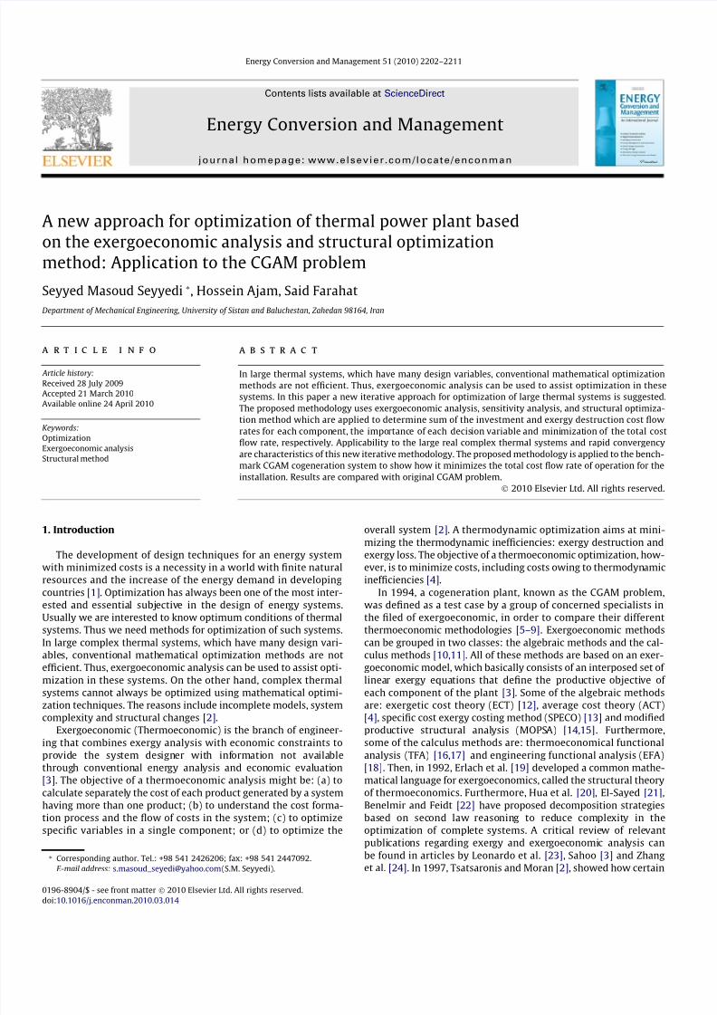
In the final analysis, the aim of CGAM problem was the unificationof exergoeconomic methodologies [3]. The CGAM system refers to
a cogeneration plant which delivers 30 MW of electricity and
14 kg sÀ1 of saturated steam at 20 bar. A schematic of cogeneration
plant is shown in Fig. 1. The system consists of an air compressor
(AC), an air preheater (APH), a combustion chamber (CC), a gas-tur-
bine (GT) and a heat-recovery steam generator (HRSG). The envi-
ronment conditions are defined as T 0 = 298.15 K and P 0 = 1.013 bar.
The objective function is the total cost flow rate of operation for
the installation that is obtained from
_C T ¼ _mf c f LHV þX5
i¼1
_ Z i ð1Þ
where C ˙ T ($/s) is the total cost flow rate of fuel and equipment and_
Z i in ($/s) is the cost flow rate associated with capital investmentand the maintenance cost for the ith component (i = AC, CC, GT,
APH, HRSG).
Also, exergetic efficiency of the cycle (gII) is defined as:
gII ¼_W net þ _msðe9 À e8Þ
_mf ef
ð2Þ
The key design variables, (the decision variables), for the cogen-
eration system are the compressor pressure ratio PR, the isentropic
compressor efficiency gAC, the isentropic turbine efficiency gGT, the
temperature of the air entering the combustion chamber T 3, and
the temperature of the combustion products entering the gas tur-
bine T 4. The objective is to minimize Eq. (1) subject to the con-
straints imposed by the physical, thermodynamic and cost
models of the installation. For more details see Appendix A andRef. [5].
Nomenclature
c cost per exergy unit ($/kJ)C ˙ exergetic cost flow rates ($/s)com componentCRF capital recovery factorE ˙ exergy flow rate (kW)
i ith plant component_I irreversibility rate (kW)
j jth decision variableLHV lower heating value of fuel (kJ/kg)_m mass flow rate
N number of the hours of plant operation per year (h/year) p parameter for sensitivity analysis, expressions (5) and
(6)PR pressure ratioT temperature (K)_W net net work of the cycle (kW)
x decision variable X vector of decision variables Z purchase costs of the ith component ($),_ Z investment cost flow rate ($/s)
Greek lettersa user – prescribed tolerance for the iterative process, Eq.
(7)e component exergetic efficienciesf capital cost coefficient
g isentropic efficiencygII exergetic efficiency of the cyclel defined in Eq. (8)r coefficient of structural bondsu maintenance factor
Subscripts0 index for environment (reference state)AC air compressorAPH air preHeaterCC combustion chamberD destructionf fuelGT gas-turbineHRSG heat-recovery steam generatorIn inletIter iterationk kth plant componentL lowerOPT optimumOut outletP productS steamT totalU upper
S.M. Seyyedi et al. / Energy Conversion and Management 51 (2010) 2202–2211 2203
8/6/2019 Seyyedi_2010_optimization of TPP Based on Ex Ergo Economic Analysis and Structural Optimization
http://slidepdf.com/reader/full/seyyedi2010optimization-of-tpp-based-on-ex-ergo-economic-analysis-and-structural 3/10
3. Structural optimization method
The purpose of this optimization is to determine the capital cost
of a selected component (system element) corresponding to the
minimum annual operating cost of the plant with a given plant
output and thus, by implication, corresponding to the minimum
unit cost of the product [27]. The following relation for the kth
component must be satisfied until the total cost flow rate of oper-
ation for the installation, C ˙ T , be minimized:
@ _I k@ xi
!OPT
¼ À1
c Ik;i
@ _ Z k@ xi
!ð3Þ
In the proposed methodology, Eq. (3) is numerically calculated
using Newton’s finite difference formula:
_I kð xi þ 1Þ À _I kð xiÞ
D xi ! ¼ À
1
c Ik;i
_ Z kð xiþ1Þ À _ Z kð xiÞ
D xi ! ð4Þ
where D xi ¼ xi þ 1 À xi . For more details see Appendix B and Ref.
[27].
4. Proposed iterative methodology
In this paper, we have proposed a new approach for optimiza-
tion of complex thermal power plant. It is worth to mention that
structural optimization method (see Section 3 and Appendix B) is
a method of optimization for one component of the system, so that
the total cost flow rate of the system to be minimized while we
have applied it for optimization of complex thermal power plant
using exergoeconomic analysis (here, ACT method [4]) and numer-
ical sensitivity analysis.
4.1. Numerical sensitivity analysis
A numerical sensitivity analysis is performed for each design
variable (decision variable) in order to determine the importance
of each decision variable. The sensitivity analysis is performed
for each xi according to the following procedure:
if xiD xi
DgII
gII
> p; xi affects exergetic efficiency; and ð5Þ
if xiD xi
D _C T_C T
> p; xi affects total cost flow rate of the system
ð6Þ
Thus, each decision variable will be settled in one of the follow-
ing groups:
Group 1: if decision variable affects both C ˙ T and gII.
Group 2: if decision variable affects on the C ˙ T only.
Group 3: if decision variable affects on the gII only.
Group 4: if decision variable affects neither C ˙ T nor gII.
The left-hand sides of expressions (5) and (6) are numerically
evaluated and compared to the value of the parameter p where
p ¼ 0:1 xi=D xi.
4.2. Algorithm for the proposed iterative methodology
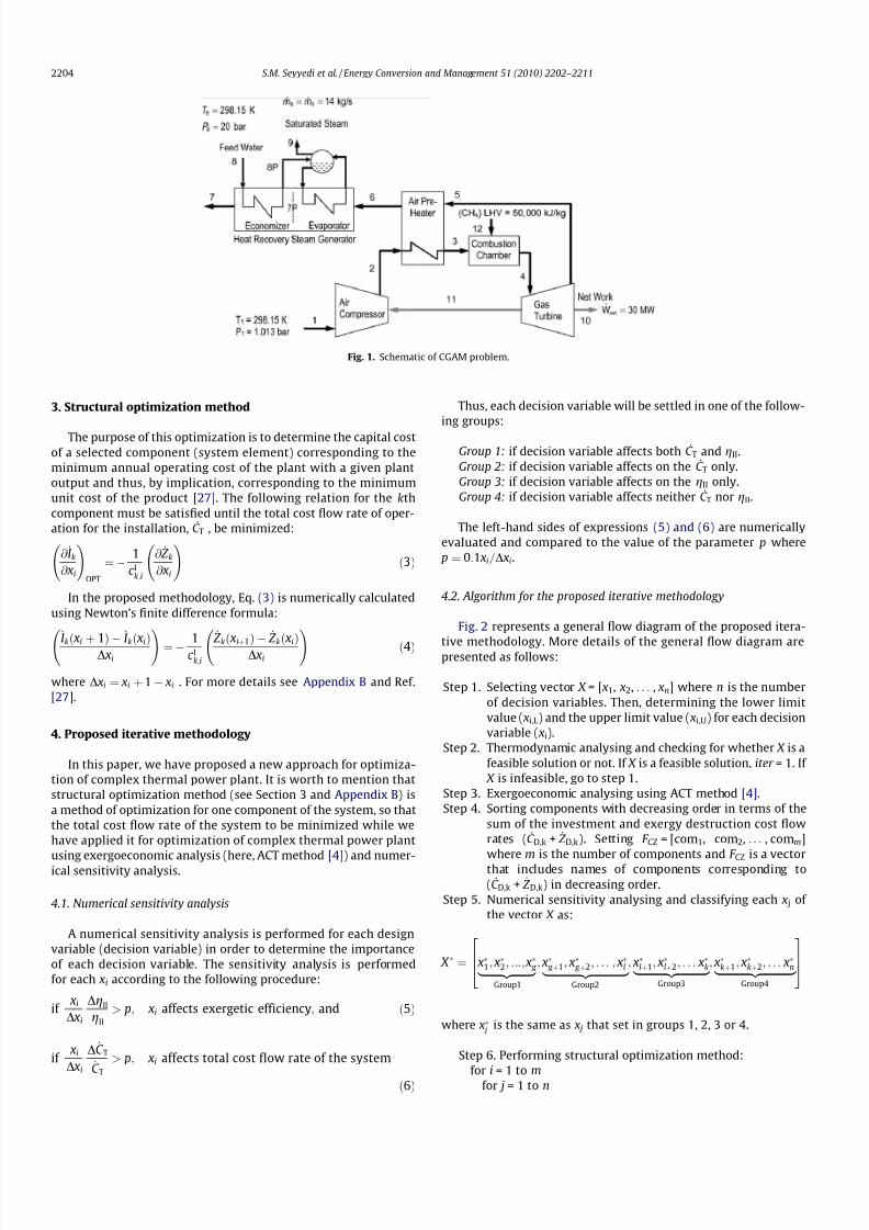
Fig. 2 represents a general flow diagram of the proposed itera-
tive methodology. More details of the general flow diagram arepresented as follows:
Step 1. Selecting vector X = [ x1, x2, . . . , xn] where n is the number
of decision variables. Then, determining the lower limit
value ( xi,L ) and the upper limit value ( xi,U) for each decision
variable ( xi).
Step 2. Thermodynamic analysing and checking for whether X is a
feasible solution or not. If X is a feasible solution, iter = 1. If
X is infeasible, go to step 1.
Step 3. Exergoeconomic analysing using ACT method [4].
Step 4. Sorting components with decreasing order in terms of the
sum of the investment and exergy destruction cost flow
rates (C ˙ D,k + _ Z D,k). Setting F CZ = [com1, com2, . . . , comm]
where m is the number of components and F CZ is a vector
that includes names of components corresponding to
(C ˙ D,k + _ Z D,k) in decreasing order.
Step 5. Numerical sensitivity analysing and classifying each x j of
the vector X as:
X Ã ¼ xÃ1; x
Ã2; :::; x
à g |fflfflfflfflfflfflfflffl{zfflfflfflfflfflfflfflffl}
Group1
; xà g þ1; x
à g þ2; . . . ; xÃ
l |fflfflfflfflfflfflfflfflfflfflfflfflffl{zfflfflfflfflfflfflfflfflfflfflfflfflffl} Group2
; xÃlþ1; x
Ãlþ2; . . . xÃ
k |fflfflfflfflfflfflfflfflfflfflffl{zfflfflfflfflfflfflfflfflfflfflffl} Group3
; xÃkþ1; x
Ãkþ2; . . . xÃ
n |fflfflfflfflfflfflfflfflfflfflfflffl{zfflfflfflfflfflfflfflfflfflfflfflffl} Group4
264
375
where xà j is the same as x j that set in groups 1, 2, 3 or 4.
Step 6. Performing structural optimization method:
for i = 1 to m
for j = 1 to n
Fig. 1. Schematic of CGAM problem.
2204 S.M. Seyyedi et al. / Energy Conversion and Management 51 (2010) 2202–2211
8/6/2019 Seyyedi_2010_optimization of TPP Based on Ex Ergo Economic Analysis and Structural Optimization
http://slidepdf.com/reader/full/seyyedi2010optimization-of-tpp-based-on-ex-ergo-economic-analysis-and-structural 4/10
6.i.j. For the ith element of F CZ (comi) and the jth element
of vector X Ãð xà j Þ , structural optimization is implemented. Thus,
xà j is updated and replaced by this value in vector X Ã.
end
Vector X Ã is updated which is called X com,i.
end
Step 7. Checking for convergency:
7.1. X Ã is named X iter and total cost flow rate (C ˙ T) is calculated
and named C ˙ T,iter.
7.2. The final vector of X (here, X com,m) is named X iter+1 and total
cost flow rate (C ˙ T) is calculated and named C ˙ T,iter+1.
7.3. Checking the following inequality:
_C T ; iterþ1 À _C T ; iter
_C T ; iter
< a ð7Þ
If Eq. (7) is satisfied, X iter+1 is the optimum solution otherwise, X is
replaced by X iter+1 and the procedure is repeated from step 3 and set
iter = iter + 1.
In Eq. (7), a is a small positive value.
It should be noted that step 5 is preformed in order to assist ra-
pid convergency.
4.3. Application to the CGAM problem
In order to represent how this proposed methodology optimizesthermal power plant, CGAM problem is selected as a test case. All
codes for calculations were developed in MATLAB. For each deci-
sion variable xi, the lower ( xi,L ) and the upper ( xi,U) limiting values
should be determined with predefined steps that have been pre-
sented in Table 1. The following steps are performed respectively:
Step 1. A vector of decision variables is randomly selected.
X ¼ ½PR; T 3; T 4;g AC ;gGT �
For each decision variable ( xi), the lower limit value ( xi,L ) and the
upper limit value ( xi,U) should be determined.
Step 2. A Thermodynamic analysis is performed to determine
whether X is a feasible solution or not. If X is a feasiblesolution iter = 1. If X is infeasible, go to step 1.
Start
Select X = [ x 1, x 2 , …. x n]
Evaluate objective function, i.e. total cost flow rate (Ċ T) by X
Exergoeconomic analysis (ACT method)
& Evalue (Ċ D,k + Ż D,k) for each component
Evaluate objective function, i.e. total cost flow rate ( T) by X new
Numerical sensitivity analysis and classify each x j in vector X that
],...,,,...,,,...,,,,...,,[
4
**2
*1
3
**2
*1
2
**2
*1
1
**2
*1
*
Group
nk k
Group
k ll
Group
Lgg
Group
g x x x x x x x x x x x x X ++++++=
STOP
NO
Yes
ConvergenceCriteria?
Components are ranked in decreasing order in terms of the sum of the investment andexergy destruction cost flow rates (Ċ D,k + Ż D,k), i.e. F CZ = [com1, com2,…,comm]
Print optimum vector ( X OPT ) & optimum total cost flow rate Ċ T,OPT
For all components of Vector F CZ & all decision variables of vector X * Perform Structural Optimization
X replaced by Xnew
Fig. 2. General flow diagram of the proposed iterative methodology.
Table 1
The lower and the upper limiting values and steps for the decision variables of the
CGAM cogeneration system.
Variable Value Step
Minimum Maximum
PR 5 25 0.01
T 3 (K) 500 1200 0.5
T 4 (K) 1200 1800 0.5
gAC 0.7 0.9 0.0001
gGT 0.7 0.92 0.0001
S.M. Seyyedi et al. / Energy Conversion and Management 51 (2010) 2202–2211 2205
8/6/2019 Seyyedi_2010_optimization of TPP Based on Ex Ergo Economic Analysis and Structural Optimization
http://slidepdf.com/reader/full/seyyedi2010optimization-of-tpp-based-on-ex-ergo-economic-analysis-and-structural 5/10
8/6/2019 Seyyedi_2010_optimization of TPP Based on Ex Ergo Economic Analysis and Structural Optimization
http://slidepdf.com/reader/full/seyyedi2010optimization-of-tpp-based-on-ex-ergo-economic-analysis-and-structural 6/10
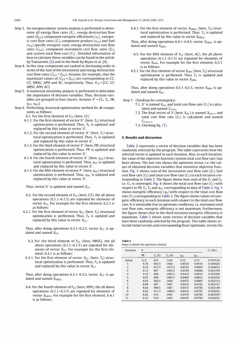
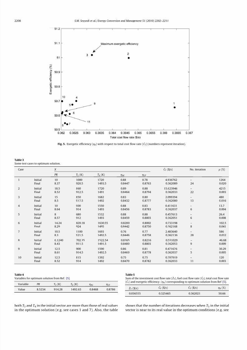
each case. In addition, the value of the objective function
(system total cost flow rate) in each case has been represented. lin the last column shows the percent of relative error of the
optimum solution results from Ref. [5] and the total cost flow rate
(C ˙ T) from the present work that is calculated by the followingequation:
l ¼_C T À _C T;OPT
_C T;OPT
! 100 ð8Þ
where_
C T ;OPT is the optimum solution from Ref. [5] (see Tables 4 and5). Table 3 also shows that the number of iterations increases when
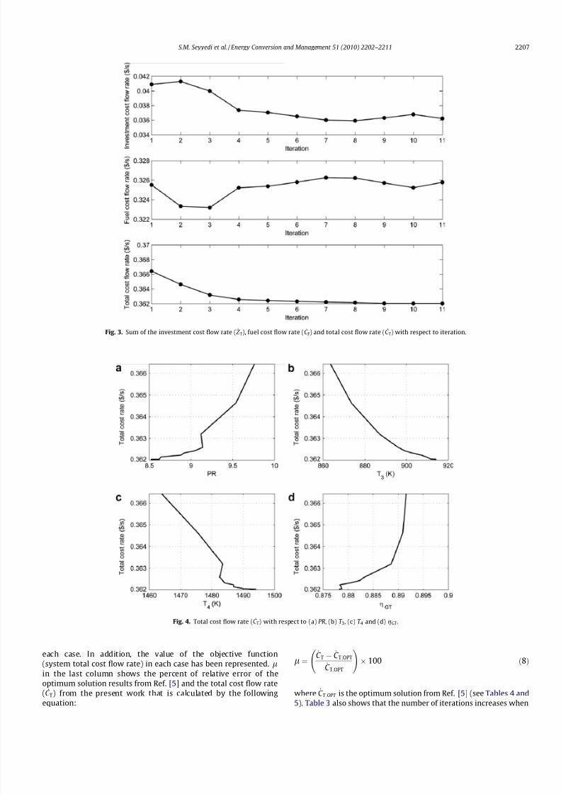
Fig. 3. Sum of the investment cost flow rate ( _ Z T), fuel cost flow rate (C ˙ F) and total cost flow rate (C ˙ T) with respect to iteration.
Fig. 4. Total cost flow rate (C ˙ T) with respect to (a) PR, (b) T 3, (c) T 4 and (d) gGT.
S.M. Seyyedi et al. / Energy Conversion and Management 51 (2010) 2202–2211 2207
8/6/2019 Seyyedi_2010_optimization of TPP Based on Ex Ergo Economic Analysis and Structural Optimization
http://slidepdf.com/reader/full/seyyedi2010optimization-of-tpp-based-on-ex-ergo-economic-analysis-and-structural 7/10
both T 3 and T 4 in the initial vector are more than those of real valuesin the optimum solution (e.g. see cases 1 and 7). Also, the table
shows that the number of iterations decreases when T 3 in the initialvector is near to its real value in the optimum conditions (e.g. see
Table 3
Some test cases to optimum solution.
Case X C ˙ T ($/s) No. iteration l (%)
PR T 3 (K) T 4 (K) gAC gGT
1 Initial 10 1000 1720 0.88 0.78 4.936762 – 1264
Final 8.37 920.5 1493.5 0.8447 0.8763 0.362089 24 0.0202 Initial 18.5 860 1720 0.89 0.88 15.623946 – 4215
Final 8.52 912.5 1491 0.8464 0.8794 0.362033 22 0.003
3 Initial 15 850 1682 0.83 0.80 2.099394 – 480
Final 8.5 917.5 1492 0.8432 0.8777 0.362080 13 0.016
4 Initial 10 900 1550 0.88 0.83 0.411631 – 13.7
Final 8.64 914 1493 0.8456 0.8783 0.362037 6 0.004
5 Initial 8 680 1532 0.88 0.88 0.457613 – 26.4
Final 8.57 912 1493 0.8459 0.8803 0.362051 6 0.008
6 Initial 14.24 820.18 1630.55 0.8280 0.8002 0.733198 – 102.5
Final 8.29 924 1495 0.8442 0.8750 0.362168 8 0.041
7 Initial 10.5 1100 1693 0.76 0.77 2.483640 – 586
Final 8.3 921.5 1492.5 0.8446 0.8758 0.362136 28 0.032
8 Initial 6.1240 702.35 1522.54 0.8365 0.8216 0.531029 – 46.68
Final 8.43 911.5 1491.5 0.8480 0.8803 0.362053 9 0.009
9 Initial 12.5 900 1590 0.86 0.81 0.471676 – 30.29
Final 8.61 914.5 1492.5 0.8460 0.8778 0.362037 5 0.005
10 Initial 12.5 815 1392 0.75 0.75 0.797919 – 120
Final 8.52 914 1492 0.8470 0.8782 0.362033 11 0.003
Table 4
Variables for optimum solution from Ref. [5].
Variable PR T 3 (K) T 4 (K) gAC gGT
Value 8.5234 914.28 1492.63 0.8468 0.8786
Table 5
Sum of the investment cost flow rate ( _ Z T), fuel cost flow rate (C ˙ F), total cost flow rate
(C ˙ T) and exergetic efficiency (gII) corresponding to optimum solution from Ref [5].
_ Z T ($/s) C ˙ F ($/s) C ˙ T ($/s) gII (%)
0.036555 0.325465 0.362021 50.66
Fig. 5. Exergetic efficiency (gII) with respect to total cost flow rate ( C ˙ T) (numbers represent iteration).
2208 S.M. Seyyedi et al. / Energy Conversion and Management 51 (2010) 2202–2211
8/6/2019 Seyyedi_2010_optimization of TPP Based on Ex Ergo Economic Analysis and Structural Optimization
http://slidepdf.com/reader/full/seyyedi2010optimization-of-tpp-based-on-ex-ergo-economic-analysis-and-structural 8/10
cases 4 and 9). Table 4 shows vector of decision variables for the
optimum conditions from Ref. [5]. Table 5 shows sum of the invest-
ment cost flow rate ( _ Z T), fuel cost flow rate (C ˙ F), total cost flow rate
(C ˙ T) and exergetic efficiency (gII) corresponding to the optimum
conditions from Ref. [5] (see Appendix A).
6. Conclusions
A new approach has been developed for the optimization of
thermal power plant based on the exergoeconomic analysis and
structural optimization. In the real complex large thermal systems
– that conventional mathematical optimization methods are not
efficient – the proposed iterative methodology is efficient for
optimization. This methodology uses exergoeconomic analysis,
sensitivity analysis, and structural optimization method. The
advantages of this new iterative methodology are: (1) it can be ap-
plied to the real complex large thermal systems; (2) the procedure
of optimization is performed without user interface, i.e. it dose not
need to the decision of designer in each iteration; and (3) since it
uses from a numerical sensitivity analysis, its convergency is rapid.
The benefits of the present work with respect to Refs. [2,23] can be
summarized as: (1) for each new iteration, new design variablesare calculated by structural optimization sub-routine (perfectly de-
scribed in Appendix B), while in Ref. [2] new design variables are
selected (and not calculated) by quality analysis of the component
with current design variable; (2) in large complex thermal systems,
(which have many design variables), it is difficult (or it is impossi-
ble) to determine which decision variable remains constant, in-
creases or decreases for the next iteration. Even if we overcome
on this problem, it is too difficult to determine the increased or de-
creased value of each decision variable; (3) since the present work
does not need any user-supplied data, this optimization can be
used widely while Ref. [2] needs to specialists of exergoeconomic
analysis for optimization; (4) a numerical sensitivity analysis is
used in the present work to achieve rapid convergency; (5) Ref.
[23] uses polyhedron method (a conventional mathematical opti-mization method) for optimization in each iteration, while present
method uses structural optimization method which is more consis-
tent with thermal systems, because of the irreversibility rate and
investment cost rate terms in Eqs. (3); and (6) although numerical
sensitivity analysis in the present work and Ref. [23] is the same,
however, the aim of the making use of it is not the same. Compar-
ison of the present results with results of original CGAM problem
test shows suitable performance and good accuracy of the pro-
posed methodology.
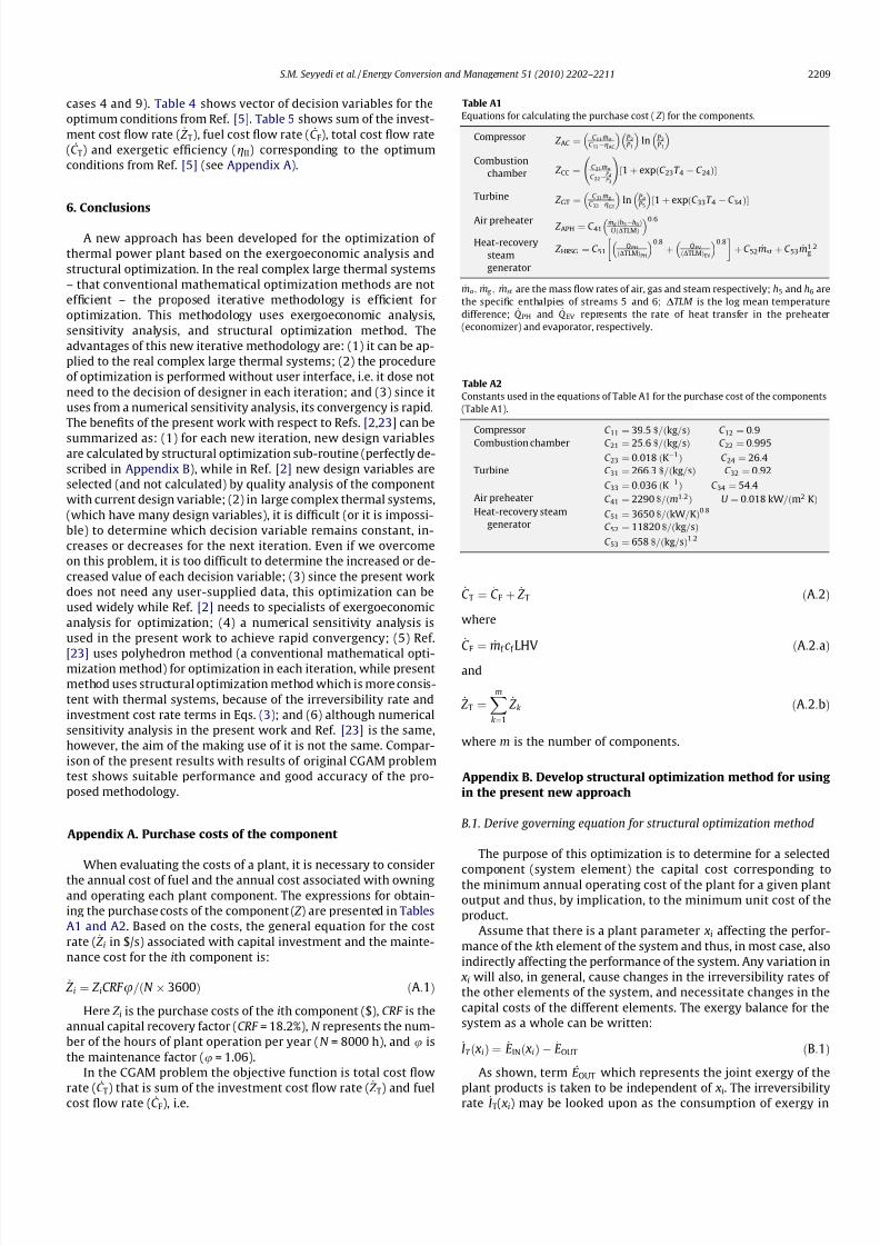
Appendix A. Purchase costs of the component
When evaluating the costs of a plant, it is necessary to consider
the annual cost of fuel and the annual cost associated with owning
and operating each plant component. The expressions for obtain-
ing the purchase costs of the component ( Z ) are presented in Tables
A1 and A2. Based on the costs, the general equation for the cost
rate ( _ Z i in $/s) associated with capital investment and the mainte-
nance cost for the ith component is:
_ Z i ¼ Z iCRF u=ðN Â 3600Þ ðA:1Þ
Here Z i is the purchase costs of the ith component ($), CRF is the
annual capital recovery factor (CRF = 18.2%), N represents the num-
ber of the hours of plant operation per year (N = 8000 h), and u is
the maintenance factor (u = 1.06).
In the CGAM problem the objective function is total cost flow
rate (C ˙ T) that is sum of the investment cost flow rate (_
Z T) and fuelcost flow rate (C ˙ F), i.e.
_C T ¼ _C F þ _ Z T ðA:2Þ
where
_C F ¼ _mf c f LHV ðA:2:aÞ
and
_ Z T ¼Xmk¼1
_ Z k ðA:2:bÞ
where m is the number of components.
Appendix B. Develop structural optimization method for using
in the present new approach
B.1. Derive governing equation for structural optimization method
The purpose of this optimization is to determine for a selected
component (system element) the capital cost corresponding tothe minimum annual operating cost of the plant for a given plant
output and thus, by implication, to the minimum unit cost of the
product.
Assume that there is a plant parameter xi affecting the perfor-
mance of the kth element of the system and thus, in most case, also
indirectly affecting the performance of the system. Any variation in
xi will also, in general, cause changes in the irreversibility rates of
the other elements of the system, and necessitate changes in the
capital costs of the different elements. The exergy balance for the
system as a whole can be written:
_I T ð xiÞ ¼ _E INð xiÞ À _E OUT ðB:1Þ
As shown, term E ˙ OUT which represents the joint exergy of the
plant products is taken to be independent of xi. The irreversibilityrate _I T( xi) may be looked upon as the consumption of exergy in
Table A1
Equations for calculating the purchase cost ( Z ) for the components.
Compressor Z AC ¼ C 11 _ma
C 12ÀgAC
P 2P 1
ln P 2
P 1
Combustion
chamber Z CC ¼ C 21 _ma
C 22ÀP 4P 3
!1 þ expðC 23T 4 À C 24Þ½ �
Turbine Z GT ¼C 31 _m g
C 32 ÀgGT ln P 4
P 5 1 þ expðC 33T 4 À C 34Þ½ �
Air preheater Z APH ¼ C 41_m g ðh5 Àh6 ÞU ðDTLMÞ
0:6
Heat-recovery
steam
generator
Z HRSG ¼ C 51_Q PH
ðDTLMÞPH
0:8þ
_Q EV
ðDTLMÞEV
0:8
þ C 52 _mst þ C 53 _m1:2g
_ma; _m g ; _mst are the mass flow rates of air, gas and steam respectively; h5 and h6 are
the specific enthalpies of streams 5 and 6; DTLM is the log mean temperature
difference; _Q PH and _Q EV represents the rate of heat transfer in the preheater
(economizer) and evaporator, respectively.
Table A2
Constants used in the equations of Table A1 for the purchase cost of the components
(Table A1).
Compressor C 11 ¼ 39:5 $=ðkg=sÞ C 12 ¼ 0:9
Combustion chamber C 21 ¼ 25:6 $=ðkg=sÞ C 22 ¼ 0:995
C 23 ¼ 0:018 ðKÀ1Þ C 24 ¼ 26:4
Turbine C 31 ¼ 266:3 $=ðkg=sÞ C 32 ¼ 0:92
C 33 ¼ 0:036 ðKÀ1Þ C 34 ¼ 54:4
Air preheater C 41 ¼ 2290 $=ðm1:2Þ U ¼ 0:018 kW=ðm2 KÞ
Heat-recovery steam
generatorC 51 ¼ 3650 $=ðkW=KÞ0:8
C 52 ¼ 11820 $=ðkg=sÞ
C 53 ¼ 658 $=ðkg=sÞ1:2
S.M. Seyyedi et al. / Energy Conversion and Management 51 (2010) 2202–2211 2209
8/6/2019 Seyyedi_2010_optimization of TPP Based on Ex Ergo Economic Analysis and Structural Optimization
http://slidepdf.com/reader/full/seyyedi2010optimization-of-tpp-based-on-ex-ergo-economic-analysis-and-structural 9/10
the system, necessary to generate the product exergy EOUT. An in-
crease in exergy consumption will necessitate corresponding to
additional exergy input, DE ˙ IN( xi).
The nature of the techniquerequires that the exergy input to the
plant should have a single fixed unit cost. This condition can be sat-
isfied by a single form of exergy input of invariable quality, e.g. fuel
or electric energy. Alternatively, theinputcouldbe made up of more
than one form of exergy of invariable quality in fixed proportions.The objective function is the total cost flow rate of operation for
the installation that is obtained from:
_C Tð xiÞ ¼ c IN_E INð xiÞ þ
Xml¼1
_ Z lð xiÞ ðB:2Þ
where C ˙ T is the total cost flow rate of fuel and equipment ($/s) and_Zl in ($/s) is the cost flow rate associated with capital investment
and the maintenance cost for the ith component.
Subject to the usual mathematical conditions being fulfilled, the
objective will be differentiated with respect to xi. From (B.1):
@ _E IN
@ xi¼
@ _I T@ xi
ðB:3Þ
So:
@ _C T@ xi
¼ c IN@ _I T@ xi
þXml¼1
@ _ Z l@ xi
ðB:4Þ
The second term on the RHS of (B.4) may be rearranged conve-
niently as:
Xml¼1
@ _ Z l@ xi
¼Xml0¼1
@ _ Z l0
@ xiþ
@ _ Z k@ xi
ðB:5Þ
where l0–k , i.e. subscript l
0 marks any of the element of the system
except that one which is subject to the optimization. Also, it will be
convenient to make the rearrangement:
Xml0 ¼1
@ _ Z l0
@ xi¼ @ _I k
@ xi
Xml0¼1
@ _ Z l0
@ _I k
!¼ @ _I k
@ xifk;i ðB:6Þ
where
fk;i ¼Xml0¼1
@ _ Z l0
@ _I k
! xi¼var; l0–k
ðB:7Þ
fk,i is the capital cost coefficient.
The coefficient of structural bonds (CSB) is defined by:
rk;i ¼
@ _I T@ xi
@ _I k@ xi
ðB:8:aÞ
Alternatively
rk;i ¼@ _I T
@ _I k
! xi¼var
ðB:8:bÞ
From (B.8-a)
@ _I T@ xi
¼ rk;i
@ _I k@ xi
!ðB:9Þ
Using (B.5)–(B.9), Eq. (B.4) can be modified as:
@ _C T@ xi
¼ c Ik;i@ _I T@ xi
þ@ _ Z k@ xi
ðB:10Þ
where
c I k;i ¼ c INrk;i þ fk;i ðB:11Þ
For optimization, set equation (B.10) equal zero. Thus:
@ _I k@ xi
!OPT
¼ À1
c Ik;i
@ _ Z k@ xi
!ðB:12Þ
B.2. Numerical solution of Eq. (B.12)
In this section, it has been described how Eq. (B.12) can be ap-
plied for structural optimization. Consider kth component and ith
decision variable. xi is ith decision variable that sets between xiL < -
xi < xiU with a step size D xi
Eq. (B.12) is numerically calculated using Newton’s finite differ-
ence formula as:
_I kð xiþ1Þ À _I kð xiÞ
D xi
!¼ À
1
c Ik;i
_ Z kð xiþ1Þ À _ Z kð xiÞ
D xi
!ðB:13Þ
where D xi ¼ xiþ1 À xi. Consider:
f 1 ¼_I kð xiþ1Þ À _I kð xiÞ
D xi
!ðB:14Þ
and
f 2 ¼ À1
c Ik;i
_ Z kð xiþ1Þ À _ Z kð xiÞ
D xi
!ðB:15Þ
Thus, when Eq. (B.13) is numerically evaluated, it can be written as:
f ¼ j f 1 À f 2j ðB:16Þ
If f ffi 0, then xi is obtained. Note that c Ik;i is numerically calcu-
lated for each xi. Fig. B1 shows functions f 1 and f 2 with respect to
xi (see Ref. [27]).
References
[1] Silveira JL, Tuna CE. Thermoeconomic analysis method for optimization of combined heat and power systems. Part I Prog Energy Combust Sci2003;29:479–85.
[2] Tsatsaronis G, Moran M. Exergy-aided cost minimization. Energy ConversManage 1997;38(15):1535–42.
[3] Sahoo PK. Exergoeconomic analysis and optimization of a cogeneration systemusing evolutionary programming. Appl Therm Eng 2008;28:1580–8.
[4] Bejan A, Tsatsaronis G, Moran M. Thermal design and optimization. NewYork: Wiley; 1996.
f 2 f 1
xi x
Fig. B1. Functions f 1 and f 2 with respect to x.
2210 S.M. Seyyedi et al. / Energy Conversion and Management 51 (2010) 2202–2211
8/6/2019 Seyyedi_2010_optimization of TPP Based on Ex Ergo Economic Analysis and Structural Optimization
http://slidepdf.com/reader/full/seyyedi2010optimization-of-tpp-based-on-ex-ergo-economic-analysis-and-structural 10/10