SHADE MUTATION STRATEGY ANALYSIS VIA DYNAMIC

SIMULATION IN COMPLEX NETWORK

Adam Viktorin

Roman Senkerik

Michal Pluhacek

Tomas Kadavy

Tomas Bata University in Zlin, Faculty of Applied Informatics

Nam T.G. Masaryka 5555, 760 01 Zlin, Czech Republic

{aviktorin, senkerik, pluhacek, kadavy}@fai.utb.cz

KEYWORDS

Differential Evolution, SHADE, Complex Network,

Mutation

ABSTRACT

This paper presents a novel approach to visualizing

Evolutionary Algorithm (EA) dynamic in complex

network and analyses the greediness of “current-to-

pbest/1” mutation strategy used in state-of-art

Differential Evolution (DE) algorithm – Success-

History based Adaptive DE (SHADE) on CEC2015

benchmark set of test functions. Provided analysis

suggests that the greediness might not be the optimal

approach for guiding the evolution.

INTRODUCTION

Differential Evolution (DE) is an algorithm for

numerical optimization, which was introduced to the

world by Storn and Price in 1995 (Storn and Price

1995). Its ingenuity and simplicity made it an

Evolutionary Algorithm (EA) with one of the largest

research community and therefore, continuous research

provided various improvements to the original

algorithm that led to one of the best performing EA

branches. DE research was summarized in (Neri and

Tirronen 2010; Das et al. 2016). Over the last decade,

variants of the DE algorithm have won numerous

numerical optimization competitions (Brest et al. 2006;

Qin et al. 2009; Das et al. 2009; Mininno et al. 2011;

Mallipeddi et al. 2011; Brest et al. 2013; Tanabe and

Fukunaga 2014) and the common denominator since

2013 is Success-History based Adaptive DE (SHADE),

which is an algorithm developed by Tanabe and

Fukunaga (Tanabe and Fukunaga 2013). SHADE is

based on the JADE algorithm by Zhang and Sanderson

(Zhang and Sanderson 2009) and belongs to the family

of adaptive DE algorithms. Adaptive algorithms are

algorithms that adapt their control parameters during the

optimization process and do not require user to set them

at the beginning, thus these algorithms are more robust

and do not require fine-tuning of the control parameters

for given problem.

SHADE algorithm uses the “current-to-pbest/1”

mutation strategy inherited from JADE, which

combines four individuals in the population. One of

them is selected greedily from the smaller subset of best

individuals, in terms of objective function value, in the

current population.

The dynamic of the SHADE algorithm is in this paper

transformed into the complex network and the greedy

behavior of the mutation strategy is analyzed with the

help of complex network feature – node centrality

value. Whereas in previous work (Viktorin et al. 2016;

Pluhacek et al. 2016) edges in complex network were

undirected and unweighted, this paper proposes an

approach with weighted and directed edges to better

capture the dynamic of the heuristic. Weights are based

on the individual donations in mutation and crossover

and directed from the donator to the beneficiary. This

approach is tested on CEC2015 benchmark set of 15 test

functions and the results of the analysis are provided

and discussed.

The remainder of the paper is structured as follows:

Next two sections describe DE and SHADE algorithms,

section that follows is about complex network design,

experiment setting and results are provided in two

following sections and the paper is concluded in the last

section.

DIFFERENTIAL EVOLUTION

The DE algorithm is initialized with a random

population of individuals P, that represent solutions of

the optimization problem. The population size NP is set

by the user along with other control parameters –

scaling factor F and crossover rate CR. In continuous

optimization, each individual is composed of a vector x

of length D, which is a dimensionality (number of

optimized attributes) of the problem, where each vector

component represents a value of the corresponding

attribute, and the individual also contains the objective

function value f(x). For each individual in a population,

three mutually different individuals are selected for

mutation of vectors and resulting mutated vector v is

combined with the original vector x in crossover step.

The objective function value f(u) of the resulting trial

vector u is evaluated and compared to that of the

original individual. When the quality (objective function

value) of the trial individual is better, it is placed into

Proceedings 31st European Conference on Modelling and Simulation ©ECMS Zita Zoltay Paprika, Péter Horák, Kata Váradi, Péter Tamás Zwierczyk, Ágnes Vidovics-Dancs, János Péter Rádics (Editors) ISBN: 978-0-9932440-4-9/ ISBN: 978-0-9932440-5-6 (CD)

the next generation, otherwise, the original individual is

placed there. This step is called selection. The process is

repeated until the stopping criterion is met (e.g. the

maximum number of objective function evaluations, the

maximum number of generations, the low bound for

diversity between objective function values in

population).

Initialization

As aforementioned, the initial population P, of size NP,

of individuals is randomly generated. For this purpose,

the individual vector xi components are generated by

Random Number Generator (RNG) with uniform

distribution from the range which is specified for the

problem by lower and upper bounds (1).

𝒙𝑗,𝑖 = 𝑈[𝑙𝑜𝑤𝑒𝑟𝑗 , 𝑢𝑝𝑝𝑒𝑟𝑗] for 𝑗 = 1, … , 𝐷 (1)

where i is the index of a current individual, j is the index

of current attribute and D is the dimensionality of the

problem.

In the initialization phase, the scaling factor value F and

the crossover rate value CR has to be assigned as well.

The typical range for F value is [0, 2] and for CR, it is

[0, 1].

Mutation

In the mutation step, three mutually different individuals

xr1, xr2, xr3 are randomly selected from a population and

combined in mutation according to the mutation

strategy. The original mutation strategy of canonical DE

is “rand/1” and is depicted in (2).

𝒗𝑖 = 𝒙𝑟1 + 𝐹(𝒙𝑟2 − 𝒙𝑟3) (2)

where r1 ≠ r2 ≠ r3 ≠ i, F is the scaling factor value and

vi is the resulting mutated vector.

Crossover

In the crossover step, mutated vector vi is combined

with the original vector xi and they produce trial vector

ui. The binomial crossover (3) is used in canonical DE.

𝑢𝑗,𝑖 = {𝑣𝑗,𝑖 if 𝑈[0,1] ≤ 𝐶𝑅 or 𝑗 = 𝑗𝑟𝑎𝑛𝑑

𝑥𝑗,𝑖 otherwise(3)

where CR is the used crossover rate value and jrand is an

index of an attribute that has to be from the mutated

vector vi (ensures generation of a vector with at least

one new component).

Selection

The selection step ensures, that the optimization

progress will lead to better solutions because it allows

only individuals of better or at least equal objective

function value to proceed into the next generation G+1

(4).

𝒙𝑖,𝐺+1 = {𝒖𝑖,𝐺 if 𝑓(𝒖𝑖,𝐺) ≤ 𝑓(𝒙𝑖,𝐺)

𝒙𝑖,𝐺 otherwise(4)

where G is the index of current generation.

The whole DE algorithm is depicted in pseudo-code

below.

Algorithm pseudo-code 1: DE

1. Set NP, CR, F and stopping

criterion;

2. G = 0, xbest = {};

3. Randomly initialize (1) population

P = (x1,G,…,xNP,G);

4. Pnew = {}, xbest = best from

population P;

5. while stopping criterion not met

6. for i = 1 to NP do

7. xi,G = P[i];

8. vi,G by mutation (2);

9. ui,G by crossover (3);

10. if f(ui,G) < f(xi,G) then

11. xi,G+1 = ui,G;

12. else

13. xi,G+1 = xi,G;

14. end

15. xi,G+1 → Pnew;

16. end

17. P = Pnew, Pnew = {}, xbest = best

from population P;

18. end

19. return xbest as the best found

solution

SUCCESS-HISTORY BASED ADAPTIVE

DIFFERENTIAL EVOLUTION

In SHADE algorithm, the only control parameter that

can be set by the user is the population size NP. Other

two (F, CR) are adapted to the given optimization task,

and a new parameter H is introduced, which determines

the size of F and CR value memories. The initialization

step of the SHADE is, therefore, similar to DE.

Mutation, however, is completely different because of

the used strategy “current-to-pbest/1” and the fact, that

it uses different scaling factor value Fi for each

individual. Crossover is still binomial, but similarly to

the mutation and scaling factor values, crossover rate

value CRi is also different for each individual. The

selection step is the same and therefore following

sections describe only different aspects of initialization,

mutation and crossover steps.

Initialization

As aforementioned, initial population P is randomly

generated as in DE, but additional memories for F and

CR values are initialized as well. Both memories have

the same size H and are equally initialized. The memory

for CR values is titled MCR and the memory for F is

titled MF. Their initialization is depicted in (5).

𝑀𝐶𝑅,𝑖 = 𝑀𝐹,𝑖 = 0.5 for 𝑖 = 1, … , 𝐻 (5)

Also, the external archive of inferior solutions A is

initialized. Since there are no solutions so far, it is

initialized empty A = Ø and its maximum size is set to

NP.

Mutation

Mutation strategy “current-to-pbest/1” was introduced

in (Zhang and Sanderson 2009) and unlike “rand/1”, it

combines four mutually different vectors, therefore

pbest ≠ r1 ≠ r2 ≠ i (6).

𝒗𝑖 = 𝒙𝑖 + 𝐹𝑖(𝒙𝑝𝑏𝑒𝑠𝑡 − 𝒙𝑖) + 𝐹𝑖(𝒙𝑟1 − 𝒙𝑟2) (6)

where xpbest is randomly selected from the best NP × p

best individuals in the current population. The p value is

randomly generated for each mutation by RNG with

uniform distribution from the range [pmin, 0.2] (Tanabe

and Fukunaga, 2013), where pmin = 2/NP. Vector xr1 is

randomly selected from the current population and

vector xr2 is randomly selected from the union of current

population P and archive A. The scaling factor value Fi

is given by (7).

𝐹𝑖 = 𝐶[𝑀𝐹,𝑟 , 0.1] (7)

where MF,r is a randomly selected value (by index r)

from MF memory and C stands for Cauchy distribution.

Therefore, the Fi value is generated from the Cauchy

distribution with location parameter value MF,r and scale

parameter value 0.1. If the generated value Fi > 1, it is

truncated to 1 and if it is Fi ≤ 0, it is generated again by

(7).

Crossover

Crossover is the same as in (3), but the CR value is

changed to CRi, which is generated separately for each

individual (8). The value is generated from the Gaussian

distribution with mean parameter value of MCR.r, which

is randomly selected (by the same index r as in

mutation) from MCR memory and standard deviation

value of 0.1.

𝐶𝑅𝑖 = 𝑁[𝑀𝐶𝑅,𝑟 , 0.1] (8)

Historical Memory Updates

Historical memories MF and MCR are initialized

according to (5), but their components change during

the evolution. These memories serve to hold successful

values of F and CR used in mutation and crossover

steps. Successful in terms of producing trial individual

better than the original individual. During one

generation, these successful values are stored in

corresponding arrays SF and SCR. After each generation,

one cell of MF and MCR memories is updated. This cell

is given by the index k, which is initialized to 1 and

increases by 1 after each generation. When k overflows

the size limit of memories H, it is reset to 1. The new

value of k-th cell for MF is calculated by (9) and for MCR

by (10).

𝑀𝐹,𝑘 = {mean𝑊𝐿(𝑺𝐹) if 𝑺𝐹 ≠ ∅

𝑀𝐹,𝑘 otherwise (9)

𝑀𝐶𝑅,𝑘 = {mean𝑊𝐴(𝑺𝐶𝑅) if 𝑺𝐶𝑅 ≠ ∅

𝑀𝐶𝑅,𝑘 otherwise (10)

where meanWL() and meanWA() are weighted Lehmer

(11) and weighted arithmetic (12) means

correspondingly.

mean𝑊𝐿(𝑺𝐹) =∑ 𝑤𝑘∙𝑆𝐹,𝑘

2|𝑺𝐹|

𝑘=1

∑ 𝑤𝑘∙𝑆𝐹,𝑘|𝑺𝐹|

𝑘=1

(11)

mean𝑊𝐴(𝑺𝐶𝑅) = ∑ 𝑤𝑘 ∙ 𝑆𝐶𝑅,𝑘

|𝑺𝐶𝑅|

𝑘=1 (12)

where the weight vector w is given by (13) and is based

on the improvement in objective function value between

trial and original individuals.

𝑤𝑘 =abs(𝑓(𝒖𝑘,𝐺)−𝑓(𝒙𝑘,𝐺))

∑ abs(𝑓(𝒖𝑚,𝐺)−𝑓(𝒙𝑚,𝐺))|𝑺𝐶𝑅|𝑚=1

(13)

And since both arrays SF and SCR have the same size, it

is arbitrary which size will be used for the upper

boundary for m in (13). Complete SHADE algorithm is

depicted in pseudo-code below.

Algorithm pseudo-code 2: SHADE

1. Set NP, H and stopping criterion;

2. G = 0, xbest = {}, k = 1, pmin =

2/NP, A = Ø;

3. Randomly initialize (1) population

P = (x1,G,…,xNP,G);

4. Set MF and MCR according to (5);

5. Pnew = {}, xbest = best from

population P;

6. while stopping criterion not met

7. SF = Ø, SCR = Ø;

8. for i = 1 to NP do

9. xi,G = P[i];

10. r = U[1, H], pi = U[pmin, 0.2];

11. Set Fi by (7) and CRi by (8);

12. vi,G by mutation (6);

13. ui,G by crossover (3);

14. if f(ui,G) < f(xi,G) then

15. xi,G+1 = ui,G;

16. xi,G → A;

17. Fi → SF, CRi → SCR;

18. else

19. xi,G+1 = xi,G;

20. end

21. if |A|>NP then randomly delete

an ind. from A;

22. xi,G+1 → Pnew;

23. end

24. if SF ≠ Ø and SCR ≠ Ø then

25. Update MF,k (9) and MCR,k (10),

k++;

26. if k > H then k = 1, end;

27. end

28. P = Pnew, Pnew = {}, xbest = best

from population P;

29. end

30. return xbest as the best found

solution

NETWORK DESIGN

The network is created for each generation of the

SHADE algorithm, where the key factors are mutation

and crossover steps. Individuals in population are nodes

in the network and edges between them are created if

the trial individual produced in mutation and crossover

succeeds in selection (has better objective function

value than the original individual). Each individual has

its own ID, trial individual ui inherits ID of the original

individual xi and therefore, the original individual and

trial individual are represented in the network by the

same node. Since there are four individuals acting in

mutation and crossover (xi, xpbest, xr1 and xr2), four edges

(ei,i, epbest,i, er1,i, er2,i) are created for each successful

selection. Each edge is directed from source to target

(donor to beneficiary) and denoted by esource,target. First

edge is a self-loop. Each edge has also its weight w,

which is denoted wsource and is based on the ratios of

donations to the trial individual. If the edge already

exists in the network, new weight is added to the current

one. Edges with their weights are depicted in Figure 1.

Figure 1: Edges Created for One Successful Evolution of an

Individual

Original individual xi donates during crossover and also

in mutation. The number of donated attributes in

crossover by xi is divided by dimension of the problem

D and the final ratio CRr (real crossover) is subtracted

from 1. This is done, because the sum of all four

weights should be 1, therefore, the cumulative value left

for the mutation donations is CRr. This value is divided

between four individuals according to their ratio in (6).

Ratios for each individual in mutation are:

xi → 1 – Fi

𝒗𝑖 = 𝒙𝑖 + 𝐹𝑖(𝒙𝑝𝑏𝑒𝑠𝑡 − 𝒙𝑖) + 𝐹𝑖(𝒙𝑟1 − 𝒙𝑟2)

xpbest → Fi

𝒗𝑖 = 𝒙𝑖 + 𝐹𝑖(𝒙𝑝𝑏𝑒𝑠𝑡 − 𝒙𝑖) + 𝐹𝑖(𝒙𝑟1 − 𝒙𝑟2)

xr1 → Fi

𝒗𝑖 = 𝒙𝑖 + 𝐹𝑖(𝒙𝑝𝑏𝑒𝑠𝑡 − 𝒙𝑖) + 𝐹𝑖(𝒙𝑟1 − 𝒙𝑟2)

xr2 → – Fi

𝒗𝑖 = 𝒙𝑖 + 𝐹𝑖(𝒙𝑝𝑏𝑒𝑠𝑡 − 𝒙𝑖) + 𝐹𝑖(𝒙𝑟1 − 𝒙𝑟2)

And each ratio is multiplied by CRr and divided by the

sum of ratios, which is 1 to obtain the proportion of CRr

as a weight. Resulting weights are depicted in (14, 15,

16 and 17).

𝑤𝑖 = (1 − 𝐶𝑅𝑟) + 𝐶𝑅𝑟 ∗ (1 − 𝐹𝑖) (14)

𝑤𝑝𝑏𝑒𝑠𝑡 = 𝐶𝑅𝑟 ∗ 𝐹𝑖 (15)

𝑤𝑟1 = 𝐶𝑅𝑟 ∗ 𝐹𝑖 (16)

𝑤𝑟2 = 𝐶𝑅𝑟 ∗ (−𝐹𝑖) (17)

where wi sums two components – crossover donation

and mutation donation. For example, if the

dimensionality of the problem D = 10, scaling factor for

this mutation Fi = 0.7 and 2 attributes are taken from the

original individual xi in crossover, then:

CRr = 2 / 10 = 0.2

wi = (1 – 0.2) + 0.2 * (1 – 0.7) = 0.86

wpbest = 0.2 * 0.7 = 0.14

wr1 = 0.2 * 0.7 = 0.14

wr2 = 0.2 * (-0.7) = -0.14

∑w = 0.86 + 0.14 + 0.14 – 0.14 = 1

EXPERIMENT SETTING

In order to obtain an analysis of the greedy behavior of

the mutation in SHADE algorithm, complex networks

were created for each generation in a SHADE run and

node centrality value (sum of weights of outgoing edges

from a node) for each individual in a population was

recorded. This was done for 15 test functions in

CEC2015 benchmark set and each test function was run

51 times with random initialization in 10D. The

stopping criterion was set to 10,000×D objective

function evaluations. The population size was set to NP

= 100 and historical memory size was set to H = 10.

The basic assumption is that the nodes, that

communicate the most (have high node centrality value)

are the ones who lead the evolution towards the global

optima. The greediness in “current-to-pbest/1” mutation

strategy is represented by xpbest individual, which is

selected from a subset of best individuals in the

population pbest (the size of this subset varies from 2

individuals to a maximum of 20% of the population

size). In theory, the pbest subset should contain

individuals leading the optimization, therefore these

individuals should correspond to the most active ones in

the network. In order to test that, a new metric

centrRank was proposed. An auxiliary variable

centrPosition is introduced and corresponds to the

number of individuals in the population that have worse

node centrality value than the current individual (e.g. If

the node has the highest centrality, than the

centrPosition value would be 99 as the number of

individuals is 100. On the other hand, if it is an

individual with worst centrality value, centrPosition

will be 0). The centrRank value is rescaled

centrPosition to the range <0, 1>, where centrPosition =

99 translates to centrRank = 1.

Values of centrRank were calculated for the subset of

20 best individuals (maximum size of pbest subset)

from the complex network created in each generation

(the complex network is pruned after that and next

generation creates a new one) and the results are

depicted in the next section.

RESULTS

This section depicts representatives of typical average

centrRank history among test functions in CEC2015

benchmark set. In the optimal scenario, the subset of 20

best individuals according to their objective function

value would be the same as the subset of 20 best

individuals according to their centrRank values and

average centrRank value in one generation would be

around 0.9. This behavior was not obtained from either

of the test functions. The closest were functions 1, 2 and

15 where there is a fast convergence to the global

(functions 1 and 2) or local optima (function 15). The

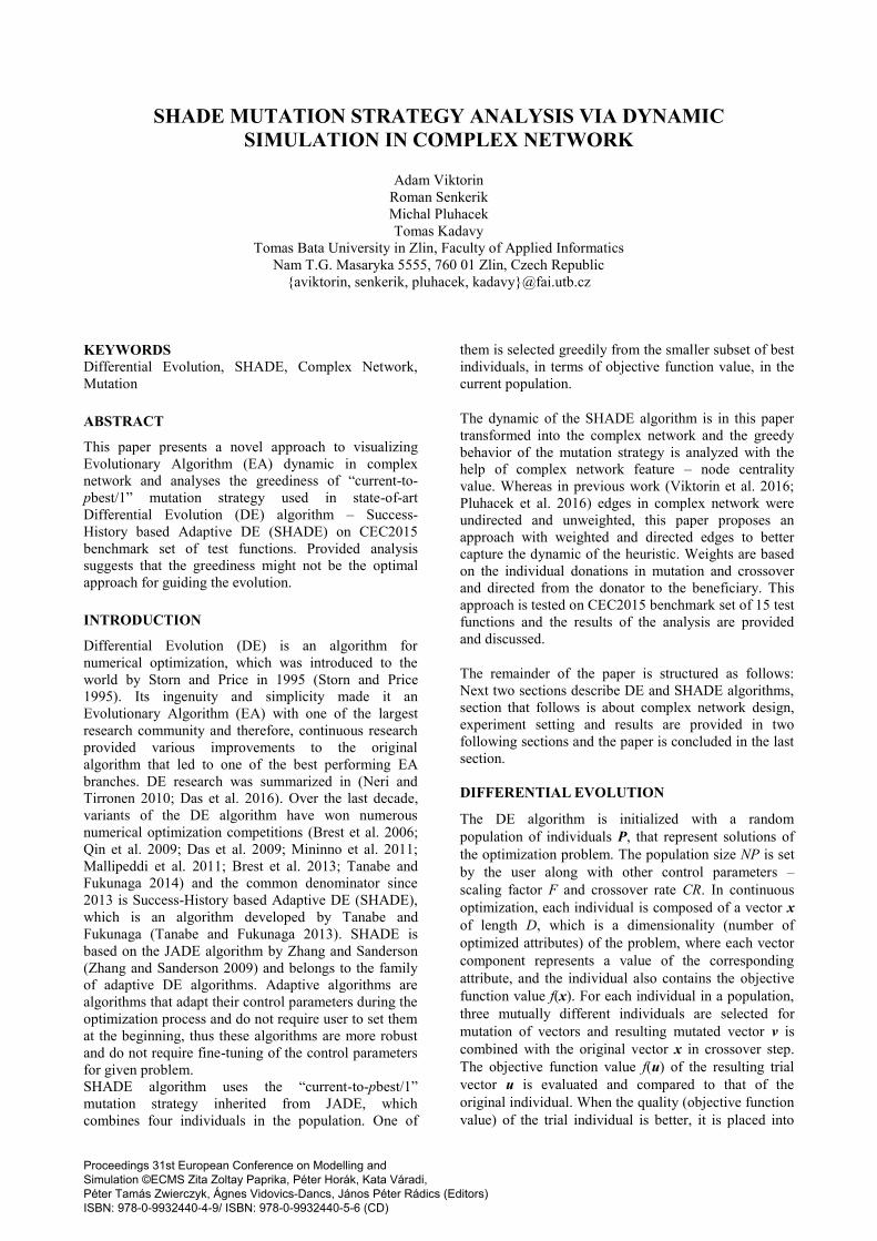
average centrRank history behavior on function 1 is

depicted in Figure 2 and convergence graph for this

function is in Figure 3.

Figure 2: CentrRank History Graph of 51 Runs on f1 in 10D

Figure 3: Convergence Graph of 51 Runs on f1 in 10D

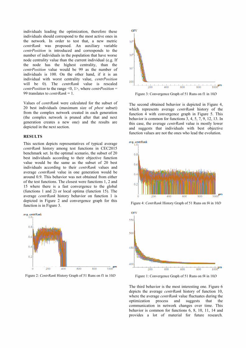
The second obtained behavior is depicted in Figure 4,

which represents average centrRank history of the

function 4 with convergence graph in Figure 5. This

behavior is common for functions 3, 4, 5, 7, 9, 12, 13. In

this case, the average centrRank value is mostly lower

and suggests that individuals with best objective

function values are not the ones who lead the evolution.

Figure 4: CentrRank History Graph of 51 Runs on f4 in 10D

Figure 1: Convergence Graph of 51 Runs on f4 in 10D

The third behavior is the most interesting one. Figure 6

depicts the average centrRank history of function 10,

where the average centrRank value fluctuates during the

optimization process and suggests that the

communication in network changes over time. This

behavior is common for functions 6, 8, 10, 11, 14 and

provides a lot of material for future research.

Convergence graph for function 10 is depicted in Figure

7.

Figure 6: CentrRank History Graph of 51 Runs on f10 in 10D

Figure 7: Convergence Graph of 51 Runs on f10 in 10D

Overall, behaviors 2 and 3 are not according to the basic

assumption and suggest that there might be a possibility

of adapting the mutation strategy to the given problem

on the basis of information from the complex network.

All average centrRank history and convergence graphs

along with numerical results can be found here:

https://owncloud.cesnet.cz/index.php/s/d59pVbT5gqXb

SrW

CONCLUSION

This work presented a novel approach for capturing

SHADE optimization process in directed and weighted

complex network, which should provide more accurate

information about the heuristic dynamic. In the

experimental part, the basic network feature – node

centrality value was used for the analysis of greedy

behavior of the “current-to-pbest/1” mutation strategy.

This analysis provided evidence that the best individuals

in population are not the ones who communicate the

most and therefore lead the evolution. This area of

research should be exploited and therefore, the future

research will be aimed at that direction. Complex

network features will be examined and used for

adaptation of the mutation strategy in order to improve

the performance of given algorithm.

ACKNOWLEDGEMENT

This work was supported by Grant Agency of the Czech

Republic – GACR P103/15/06700S, further by the

Ministry of Education, Youth and Sports of the Czech

Republic within the National Sustainability Programme

Project no. LO1303 (MSMT-7778/2014). Also by the

European Regional Development Fund under the

Project CEBIA-Tech no. CZ.1.05/2.1.00/03.0089 and

by Internal Grant Agency of Tomas Bata University

under the Projects no. IGA/CebiaTech/2017/004.

REFERENCES

Brest, J., Greiner, S., Boskovic, B., Mernik, M., & Zumer, V. (2006). Self-adapting control parameters in differential evolution: A comparative study on numerical benchmark prob-lems. IEEE transactions on evolutionary computation, 10(6), 646-657.

Brest, J., Korošec, P., Šilc, J., Zamuda, A., Bošković, B., & Maučec, M. S. (2013). Differen-tial evolution and differential ant-stigmergy on dynamic optimisation problems. International Journal of Systems Science, 44(4), 663-679.

Das, S., Abraham, A., Chakraborty, U. K., & Konar, A. (2009). Differential evolution using a neighborhood-based mutation operator. IEEE Transactions on Evolutionary Computa-tion, 13(3), 526-553.

Das, S., Mullick, S. S., & Suganthan, P. N. (2016). Recent advances in differential evolution–An updated survey. Swarm and Evolutionary Computation, 27, 1-30.

Mallipeddi, R., Suganthan, P. N., Pan, Q. K., & Tasgetiren, M. F. (2011). Differential evolu-tion algorithm with ensemble of parameters and mutation strategies. Applied Soft Compu-ting, 11(2), 1679-1696.

Mininno, E., Neri, F., Cupertino, F., & Naso, D. (2011). Compact differential evolution. IEEE Transactions on Evolutionary Computation, 15(1), 32-54.

Neri, F., & Tirronen, V. (2010). Recent advances in differential evolution: a survey and exper-imental analysis. Artificial Intelligence Review, 33(1-2), 61-106.

Pluhacek, M., Janostik, J., Senkerik, R., & Zelinka, I. (2016). Converting PSO dynamics into complex network-Initial study. In T. Simos, & C. Tsitouras (Eds.), AIP Conference Proceedings (Vol. 1738, No. 1, p. 120021). AIP Publishing.

Qin, A. K., Huang, V. L., & Suganthan, P. N. (2009). Differential evolution algorithm with strategy adaptation for global numerical optimization. IEEE transactions on Evolutionary Computation, 13(2), 398-417.

Storn, R., & Price, K. (1995). Differential evolution-a simple and efficient adaptive scheme for global optimization over continuous spaces (Vol. 3). Berkeley: ICSI.

Tanabe, R., & Fukunaga, A. (2013). Success-history based parameter adaptation for differential evolution. In Evolutionary Computation (CEC), 2013 IEEE Congress on (pp. 71-78). IEEE.

Tanabe, R., & Fukunaga, A. S. (2014). Improving the search performance of SHADE using linear population size reduction. In Evolutionary Computation (CEC), 2014 IEEE Con-gress on (pp. 1658-1665). IEEE.

Viktorin, A., Pluhacek, M., & Senkerik, R. (2016). Network Based Linear Population Size Reduction in SHADE. In Intelligent Networking and Collaborative Systems (INCoS), 2016 International Conference on (pp. 86-93). IEEE.

Zhang, J., & Sanderson, A. C. (2009). JADE: adaptive differential evolution with optional external archive. Evolutionary Computation, IEEE Transactions on, 13(5), 945-958.

AUTHOR BIOGRAPHIES

ADAM VIKTORIN was born in the Czech Republic,

and went to the Faculty of Applied

Informatics at Tomas Bata University in

Zlín, where he studied Computer and

Communication Systems and obtained his

MSc degree in 2015. He is studying his

Ph.D. at the same university and the fields

of his studies are: Artificial intelligence, data mining

and evolutionary algorithms. His email address is:

aviktorin@fai.utb.cz

ROMAN SENKERIK was born in the Czech Republic,

and went to the Tomas Bata University in

Zlin, where he studied Technical

Cybernetics and obtained his MSc degree

in 2004, Ph.D. degree in Technical

Cybernetics in 2008 and Assoc. prof. in

2013 (Informatics). He is now an Assoc.

prof. at the same university (research and courses in:

Evolutionary Computation, Applied Informatics,

Cryptology, Artificial Intelligence, Mathematical

Informatics). His email address is: senkerik@fai.utb.cz

MICHAL PLUHACEK was born in the Czech

Republic, and went to the Faculty of

Applied Informatics at Tomas Bata

University in Zlín, where he studied

Information Technologies and obtained his

MSc degree in 2011 and Ph.D. in 2016

with the dissertation topic: Modern method

of development and modifications of evolutionary

computational techniques. He now works as a

researcher at the same university. His email address is:

pluhacek@fai.utb.cz

TOMAS KADAVY was born in the Czech Republic,

and went to the Faculty of Applied

Informatics at Tomas Bata University in

Zlín, where he studied Information

Technologies and obtained his MSc degree

in 2016. He is studying his Ph.D. at the

same university and the fields of his

studies are: Artificial intelligence and evolutionary

algorithms. His email address is: kadavy@fai.utb.cz