Shading-based Refinement on Volumetric Signed Distance Functions

Michael Zollhofer1,4 Angela Dai2 Matthias Innmann1 Chenglei Wu3

Marc Stamminger1 Christian Theobalt4 Matthias Nießner21University of Erlangen-Nuremberg 2Stanford University 3ETH Zurich 4MPI Informatics

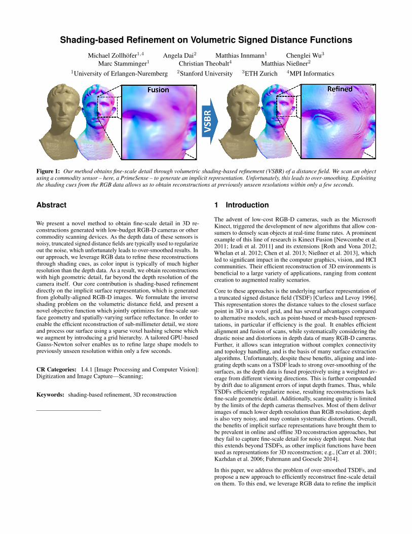
Figure 1: Our method obtains fine-scale detail through volumetric shading-based refinement (VSBR) of a distance field. We scan an objectusing a commodity sensor – here, a PrimeSense – to generate an implicit representation. Unfortunately, this leads to over-smoothing. Exploitingthe shading cues from the RGB data allows us to obtain reconstructions at previously unseen resolutions within only a few seconds.

Abstract

We present a novel method to obtain fine-scale detail in 3D re-constructions generated with low-budget RGB-D cameras or othercommodity scanning devices. As the depth data of these sensors isnoisy, truncated signed distance fields are typically used to regularizeout the noise, which unfortunately leads to over-smoothed results. Inour approach, we leverage RGB data to refine these reconstructionsthrough shading cues, as color input is typically of much higherresolution than the depth data. As a result, we obtain reconstructionswith high geometric detail, far beyond the depth resolution of thecamera itself. Our core contribution is shading-based refinementdirectly on the implicit surface representation, which is generatedfrom globally-aligned RGB-D images. We formulate the inverseshading problem on the volumetric distance field, and present anovel objective function which jointly optimizes for fine-scale sur-face geometry and spatially-varying surface reflectance. In order toenable the efficient reconstruction of sub-millimeter detail, we storeand process our surface using a sparse voxel hashing scheme whichwe augment by introducing a grid hierarchy. A tailored GPU-basedGauss-Newton solver enables us to refine large shape models topreviously unseen resolution within only a few seconds.

CR Categories: I.4.1 [Image Processing and Computer Vision]:Digitization and Image Capture—Scanning;

Keywords: shading-based refinement, 3D reconstruction

1 Introduction

The advent of low-cost RGB-D cameras, such as the MicrosoftKinect, triggered the development of new algorithms that allow con-sumers to densely scan objects at real-time frame rates. A prominentexample of this line of research is Kinect Fusion [Newcombe et al.2011; Izadi et al. 2011] and its extensions [Roth and Vona 2012;Whelan et al. 2012; Chen et al. 2013; Nießner et al. 2013], whichled to significant impact in the computer graphics, vision, and HCIcommunities. Their efficient reconstruction of 3D environments isbeneficial to a large variety of applications, ranging from contentcreation to augmented reality scenarios.

Core to these approaches is the underlying surface representation ofa truncated signed distance field (TSDF) [Curless and Levoy 1996].This representation stores the distance values to the closest surfacepoint in 3D in a voxel grid, and has several advantages comparedto alternative models, such as point-based or mesh-based represen-tations, in particular if efficiency is the goal. It enables efficientalignment and fusion of scans, while systematically considering thedrastic noise and distortions in depth data of many RGB-D cameras.Further, it allows scan integration without complex connectivityand topology handling, and is the basis of many surface extractionalgorithms. Unfortunately, despite these benefits, aligning and inte-grating depth scans on a TSDF leads to strong over-smoothing of thesurfaces, as the depth data is fused projectively using a weighted av-erage from different viewing directions. This is further compoundedby drift due to alignment errors of input depth frames. Thus, whileTSDFs efficiently regularize noise, resulting reconstructions lackfine-scale geometric detail. Additionally, scanning quality is limitedby the limits of the depth cameras themselves. Most of them deliverimages of much lower depth resolution than RGB resolution; depthis also very noisy, and may contain systematic distortions. Overall,the benefits of implicit surface representations have brought them tobe prevalent in online and offline 3D reconstruction approaches, butthey fail to capture fine-scale detail for noisy depth input. Note thatthis extends beyond TSDFs, as other implicit functions have beenused as representations for 3D reconstruction; e.g., [Carr et al. 2001;Kazhdan et al. 2006; Fuhrmann and Goesele 2014].

In this paper, we address the problem of over-smoothed TSDFs, andpropose a new approach to efficiently reconstruct fine-scale detailon them. To this end, we leverage RGB data to refine the implicit

surface representation using shading cues. Since color input is typi-cally of much higher resolution than the depth data, we can obtainreconstructions with geometric detail far beyond the depth resolu-tion of the camera itself. Operating directly on the implicit surfacerepresentation, as opposed to previous approaches on meshes, hasseveral distinct advantages. The regular structure of the TSDF natu-rally yields a spatially uniform sampling, in contrast to the overheadrequired to regularly sample a mesh. Further, we employ a sparsehashing-based scheme to store the TSDF, providing efficient storageand fast refinement. Additionally, operating on an implicit surfacerepresentation gives our approach versatility, as implicit surface rep-resentations are used in many other reconstruction approaches; e.g.,using other active triangulation sensors, laser scanning, or passiveimage-based reconstruction. In addition to geometric refinement ofconsumer RGB-D sensor input, we also demonstrate clear improve-ments in other settings in Section 7.

From globally-aligned color and depth input, we estimate the in-cident lighting distribution, and present a novel objective functionto jointly optimize for geometric refinement and dense albedo ingeneral and unconstrained environments. To solve this non-linearoptimization problem, we present a tailored, parallel Gauss-Newtonsolver. Our TSDF structure also uses a hierarchy of resolutions,which is required for efficient convergence. All our data structuresand algorithms are designed for efficient execution on the GPU.Our new refinement method is geared towards RGB-D scanning,improves over the state-of-the-art in many ways, and is based on thefollowing contributions:

• a formulation of the inverse shading problem on a TSDF, al-lowing for joint optimization of fine-scale geometric detail anddense, spatially-varying albedo (Section 5)

• an extension of the sparse voxel hashing scheme to support ahierarchy of resolutions, which provides efficient storage andfast refinement of TSDFs (Section 4)

• a GPU-based non-linear Gauss-Newton solver crafted to solvefor shading-based refinement on tens of millions of variablesin a few seconds (Section 6)

2 Related Work

Implicit functions are popular scene representations used in many3D reconstruction algorithms [Hoppe et al. 1992; Carr et al. 2001;Kazhdan et al. 2006; Fuhrmann and Goesele 2014]. Implicit modelsfacilitate partial scan alignment and integration without complextopology handling (as needed for meshes). A popular variant isthe signed distance field (SDF) model which stores distances to thesurface on a voxel grid [Curless and Levoy 1996]. It was used for off-line reconstruction of large models from partial range scans [Levoyet al. 2000], but has also been used in real-time structured lightscanning [Rusinkiewicz et al. 2002] where its efficient storage andsimple update is beneficial.

Recently, new cheap consumer-grade RGB-D cameras, such as thetriangulation-based Kinect or time-of-flight (TOF) cameras, havebecome increasingly popular for 3D scanning [Henry et al. 2012].Some hand-held RGB-D scanning approaches resort to point-basedscene models [Keller et al. 2013; Weise et al. 2009]. However,SDFs are the more widely used representation in recent real-timemethods. The Kinect Fusion algorithm [Newcombe et al. 2011;Izadi et al. 2011] was one of the first to do online alignment andintegration of RGB-D depth data using weighted averaging of par-tial scans in a truncated SDF. Several extensions of the approachwere proposed; e.g., a direct variational depth-to-SDF alignmentinstead of ICP [Bylow et al. 2013], or to use a combination of suchalignment with color optimization of aligned partial SDFs [Kehl

et al. 2014]. The SDF model also simplifies consideration of theoften drastic noise in the depth data of consumer depth cameraswhen integrating the scene model. Kinect Fusion stores the implicitmodel on a regular grid, which limits scalability to larger scenes. Toscan larger scenes, the use of shifting volumes [Whelan et al. 2012],hierarchical grids [Chen et al. 2013] or sparse voxel hashing datastructures [Nießner et al. 2013] was proposed. Unfortunately, mostRGB-D camera scanning approaches suffer from over-smoothedreconstructions due to the averaging during scan integration; thereconstructed geometric detail is thus not sufficient for many profes-sional applications. This problem is amplified by the fact that mostRGB-D cameras have a very low depth resolution, inhibiting captureof high geometric detail. Some methods attempt to overcome thedepth camera resolution limit by time-consuming multi-depth-framesuper-resolution from nearby RGB-D images [Schuon et al. 2009;Cui et al. 2010], but reconstructions are still of limited detail. Othertechniques improve depth resolution by leveraging the fact that mostRGB-D cameras have drastically higher RGB resolution than depthresolution. Another approach is to assume the alignment of colorand depth edges, which can be exploited in a joint edge-preservingupsampling filter, such as a bilateral or multi-lateral filter [Lind-ner et al. 2007; Kopf et al. 2007; Chan et al. 2008; Dolson et al.2010; Richardt et al. 2012], or explicitly phrased in an optimizationproblem [Park et al. 2011; Diebel and Thrun 2006]. Despite moredetailed and less noisy results, many of the approaches suffer fromtexture-copy artifacts since assumptions about lighting are oftenwrong and shading effects are mistaken for geometry detail. Ourapproach also exploits the higher RGB resolution of consumer depthcameras, but takes inspiration from recent progresses in scene re-construction from single or multi-view RGB images only. Recentmethods for 3D scene reconstruction from a hand-held RGB camerause a combination of sparse feature tracking, structure-from-motion,and stereo to reconstruct the scene geometry by integration in anSDF [Newcombe and Davison 2010; Pradeep et al. 2013]. How-ever, the reconstructed models show similar over-smoothing as theaforementioned RGB-D results. This is not only due to averaging inthe SDF, but also due to the stereo reconstruction itself, which oftenrequires strong regularization to find image correspondences fromscene texture [Seitz et al. 2006; Scharstein et al. 2014].

Shape-from-shading (SfS) is able to overcome some of these reso-lution limits, and also succeeds on texture-less objects [Horn 1975;Zhang et al. 1999]. SfS is well-understood, particularly when sur-face reflectance and light source positions are known [Prados andFaugeras 2005]. It can also refine coarse image-based shape models,for instance from multi-view stereo [Beeler et al. 2012], even ifthey were captured under general uncontrolled lighting with severalcameras [Wu et al. 2011; Wu et al. 2013]. To this end, illuminationand albedo distributions, as well as refined geometry, are found viainverse rendering optimizations. SfS is inherently ill-posed in un-controlled scenes, and achieving compelling results requires strongscene and lighting assumptions, as well as computationally complexalgorithms, particularly to solve hard non-linear inverse renderingoptimizations.

Several reconstruction approaches use prior models on reflectanceto alleviate some of these problems; e.g., [Haber et al. 2009]. Analternative strategy is photometric stereo, which uses images of ascene captured under different controlled illumination [Mulliganand Brolly 2004; Hernandez et al. 2008; Ghosh et al. 2011; De-bevec 2012; Nehab et al. 2005]. However, these approaches dependon complex controlled lighting setups, which are not available forscanning in general environments. Other methods create super-resolution texture maps from multi-view RGB images that werealigned on coarse image-based 3D models [Goldluecke et al. 2014];however, they do not refine reconstructed geometry. Since theyjointly consider cues from multiple aligned RGB images, many of

these image-based approaches produce results of higher detail thancurrent RGB-D camera methods, but computation times are verylong even on moderate shape resolutions.

Some methods thus combine image-based stereo and RGB-D depthfor reconstruction [Nair et al. 2013], but comparably high geometricdetail to that obtained by shading-based refinement is usually notattained. Zhou et al. [2014] combine Kinect Fusion with a texturewarping and frame bundling approach. This yields ghost-free tex-tures warped to a coarse SDF model, which means that the texturedmodel is not geometrically accurate. Recently, shape-from-shadingunder general illumination was used to up-sample and refine a singleRGB-D depth image [Han et al. 2013; Yu et al. 2013] at offline rates,and Wu et al. [2014] refine a single RGB-D camera depth frame atvideo rate. However, single frame RGB-D methods are specializedto the image domain and cannot process a 3D reconstruction. Un-fortunately, simply integrating their results in a Kinect Fusion style,causes a notable loss of the refined detail.

Current work on intrinsic image and video decomposition [Chen andKoltun 2013; Lee et al. 2012] deals with the problem of separatingalbedo and shading. These methods employ sophisticated albedoregularization strategies, but are computationally more expensiveand do not easily extend to the volume.

3 Overview

In this section, we provide a brief overview of our method. Wefirst capture input color and depth using commodity sensors (e.g.,Microsoft Kinect). This yields a sequence of depth images Diand color images Ci, which we use to generate an implicit surfacerepresenting the scanned scene (Section 4.3). We follow Curlessand Levoy [1996], and use a truncated signed distance function torepresent the implicit surface. From Di and Ci, we obtain an initialtruncated signed distance field D, from which we then solve for therefined signed distance field D. To this end, we augment each voxelv with the shading attributes – i.e., albedo a(v) and refined distanceD(v) – needed for our geometric refinement. In addition, we builda hierarchy of sparse voxel grids with varying voxel sizes to accountfor the differing depth and color input resolutions. This enablesour shading-based refinement to run efficiently in a coarse-to-finefashion. Note that to obtain sharp color data in the fused model, weoptimize for the rigid camera poses Ti bringing each frame i backto the space of the first frame (Section 4.4).

We then run our shading-based refinement on the sparse voxel hi-erarchy (Section 5). To accommodate general and uncontrolledlighting environments, we continually estimate incident irradiance.We rephrase the inverse shading problem for an implicit TSDF sur-face, simultaneously optimizing for refined surface geometry anddense, spatially-varying albedo. These dense albedos, as opposedto coarsely aligned clusters of albedos as in many previous shading-based refinement methods (e.g., [Wu et al. 2011; Wu et al. 2013]),further inform the lighting estimation and enable more accurateshape refinement results. We optimize our new objective functionwith a custom GPU-based parallel Gauss-Newton optimizer whichallows to solve for tens of millions of variables within a few seconds.This yields the refined scene model D with fine-scale detail fromthe RGB data mapped to the shape model. Fig. 2 shows an overviewof our reconstruction pipeline.

4 Implicit Surface Generation

We follow Curless and Levoy [1996], and represent surface geom-etry of a scanned scene using a truncated signed distance function(TSDF), denoted as D. The TSDF is defined as a piecewise linear

function, where supporting data is stored in a regular grid, composedof a set of voxels {vi,j,k}. Every voxel is a sampled point of D,containing a (signed) distance data point D(v). Accessing the vol-umetric distance field D for non-discrete points p ∈ R3 is donethrough tri-linear interpolation. Typically, we are interested in pointsp on the iso-surface of D, where D(p) = 0, which we will denoteas D0. Defining geometry as an implicit signed distance functionhas many advantages. A TSDF enables the regularization and noise-aware integration of noisy input depth data (e.g., obtained fromcommodity RGB-D sensors), and is a versatile representation thathas been used in many scanning pipelines and surface reconstructionapproaches. Additionally, it is easy to convert to other shape repre-sentations. Similar to Kinect Fusion [Newcombe et al. 2011; Izadiet al. 2011], we incrementally align and integrate RGB-D images toget an initial coarse signed distance field D (Section 4.3) which issubsequently geometrically refined (Section 5).

4.1 Extended Sparse Voxel Data Structure

Our ultimate goal is to obtain a refined distance field D by utilizingcolor data and shape-from-shading under general lighting conditions.We thus require a sufficiently high voxel resolution to capture allgeometric detail from RGB images. To this end, we aim to set thevoxel resolution such that the 2D projections of voxels are smallerthan the pixel size of input color images; as shown by our results,this is typically well below 1 mm3 (cf. Section 7). For efficientsurface reconstruction and refinement at this extremely high spatialresolution, we store and process all data structures on the GPU.

In addition to the signed distance value, each voxel stores values ofadditional attributes for color C(v) and integration weight W(v),both of which are explained in Section 4.3. In contrast to previouswork, our voxels also need to store additional attributes for shaperefinement (see Section 5); i.e., a luminance albedo a(v) and arefined signed distance value D(v). Our per-voxel data structureis depicted in Listing 1. Note that the requirement to store bothD and D is due to the stabilization term in our objective function(cf. Section 5.2).

The above considerations show that we reconstruct at a very high spa-tial resolution, matching high-end offline scanning systems [Levoyet al. 2000], even while book-keeping more data per voxel. Since wedo not want to sacrifice computational efficiency, we exploit the ca-pabilities of modern GPUs. To store and process this high-resolutiondata on the GPU, we store voxels sparsely using an extension ofthe voxel hashing scheme of Nießner et al. [2013]. The core ideais to use a spatial hashing function to reference a relatively smallnumber of voxel blocks close to 3D locations where the actual iso-surface resides; in our implementation, we use 43 voxel blocks.Note that a sparse representation is key to efficient storage and fastshading-based refinement.

Instead of a single, high-resolution voxel grid, as in [Nießner et al.2013], we maintain a hierarchy of sparse grids with varying voxelsizes to facilitate the later shading-based refinement. Since colorresolution is typically much higher than the corresponding inputdepth, we set the voxel resolution on the coarsest level to correspondto the input depth resolution, and the voxel size at the finest levelto correspond to the input RGB data. This enables an efficientcoarse-to-fine optimization, ultimately allowing us to obtain therefined signed distance function D at the highest resolution (seeSection 5.2). Note that our hierarchical TSDF model stores boththe initial integration result D and the final refined result D. Beforeminimizing the shading-based refinement objective (see Section 5.2),we initialize D with D.

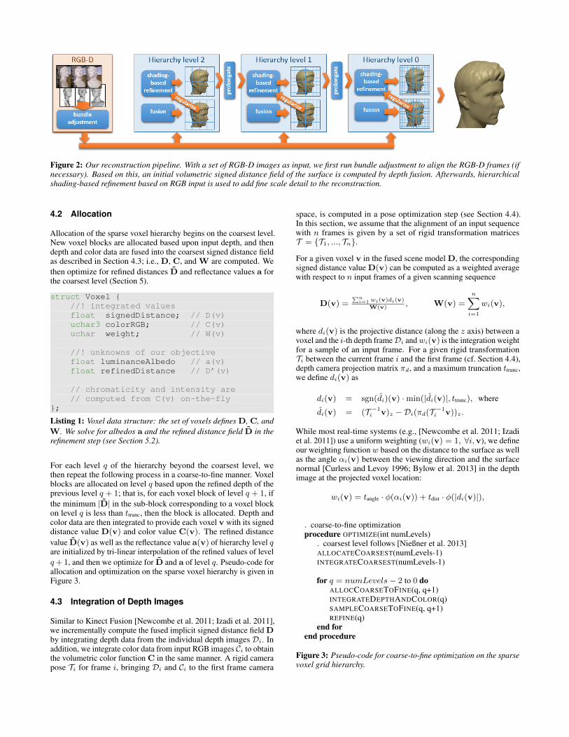
Figure 2: Our reconstruction pipeline. With a set of RGB-D images as input, we first run bundle adjustment to align the RGB-D frames (ifnecessary). Based on this, an initial volumetric signed distance field of the surface is computed by depth fusion. Afterwards, hierarchicalshading-based refinement based on RGB input is used to add fine scale detail to the reconstruction.

4.2 Allocation

Allocation of the sparse voxel hierarchy begins on the coarsest level.New voxel blocks are allocated based upon input depth, and thendepth and color data are fused into the coarsest signed distance fieldas described in Section 4.3; i.e., D, C, and W are computed. Wethen optimize for refined distances D and reflectance values a forthe coarsest level (Section 5).

struct Voxel {//! integrated valuesfloat signedDistance; // D(v)uchar3 colorRGB; // C(v)uchar weight; // W(v)

//! unknowns of our objectivefloat luminanceAlbedo // a(v)float refinedDistance // D’(v)

// chromaticity and intensity are// computed from C(v) on-the-fly

};

Listing 1: Voxel data structure: the set of voxels defines D, C, andW. We solve for albedos a and the refined distance field D in therefinement step (see Section 5.2).

For each level q of the hierarchy beyond the coarsest level, wethen repeat the following process in a coarse-to-fine manner. Voxelblocks are allocated on level q based upon the refined depth of theprevious level q + 1; that is, for each voxel block of level q + 1, ifthe minimum |D| in the sub-block corresponding to a voxel blockon level q is less than ttrunc, then the block is allocated. Depth andcolor data are then integrated to provide each voxel v with its signeddistance value D(v) and color value C(v). The refined distancevalue D(v) as well as the reflectance value a(v) of hierarchy level qare initialized by tri-linear interpolation of the refined values of levelq+ 1, and then we optimize for D and a of level q. Pseudo-code forallocation and optimization on the sparse voxel hierarchy is given inFigure 3.

4.3 Integration of Depth Images

Similar to Kinect Fusion [Newcombe et al. 2011; Izadi et al. 2011],we incrementally compute the fused implicit signed distance field Dby integrating depth data from the individual depth images Di. Inaddition, we integrate color data from input RGB images Ci to obtainthe volumetric color function C in the same manner. A rigid camerapose Ti for frame i, bringing Di and Ci to the first frame camera

space, is computed in a pose optimization step (see Section 4.4).In this section, we assume that the alignment of an input sequencewith n frames is given by a set of rigid transformation matricesT = {T1, ..., Tn}.

For a given voxel v in the fused scene model D, the correspondingsigned distance value D(v) can be computed as a weighted averagewith respect to n input frames of a given scanning sequence

D(v) =∑n

i=1 wi(v)di(v)

W(v), W(v) =

n∑i=1

wi(v),

where di(v) is the projective distance (along the z axis) between avoxel and the i-th depth frameDi andwi(v) is the integration weightfor a sample of an input frame. For a given rigid transformationTi between the current frame i and the first frame (cf. Section 4.4),depth camera projection matrix πd, and a maximum truncation ttrunc,we define di(v) as

di(v) = sgn(di)(v) ·min(|di(v)|, ttrunc), where

di(v) = (T −1i v)z −Di(πd(T −1

i v))z.

While most real-time systems (e.g., [Newcombe et al. 2011; Izadiet al. 2011]) use a uniform weighting (wi(v) = 1, ∀i,v), we defineour weighting functionw based on the distance to the surface as wellas the angle αi(v) between the viewing direction and the surfacenormal [Curless and Levoy 1996; Bylow et al. 2013] in the depthimage at the projected voxel location:

wi(v) = tangle · φ(αi(v)) + tdist · φ(|di(v)|),

. coarse-to-fine optimizationprocedure OPTIMIZE(int numLevels)

. coarsest level follows [Nießner et al. 2013]ALLOCATECOARSEST(numLevels-1)INTEGRATECOARSEST(numLevels-1)

for q = numLevels− 2 to 0 doALLOCCOARSETOFINE(q, q+1)INTEGRATEDEPTHANDCOLOR(q)SAMPLECOARSETOFINE(q, q+1)REFINE(q)

end forend procedure

Figure 3: Pseudo-code for coarse-to-fine optimization on the sparsevoxel grid hierarchy.

where tangle and tdist are user-defined constants, and φ(x) is a robustkernel with a user-defined constant trob (2 ∼ 5 in our experiments)

φ(x) = 1/(1 + trob · x)3.

The first term of w gives scene regions that are seen most head-on ahigher priority. This reflects the lower measurement uncertainty ofmost depth cameras for such regions. The second term gives valuesof voxels that are further from the surface a lower weight duringintegration. We integrate color data analogously to depth: for allRGB input frames Ci, we use the weighted average as shown above.Note that we keep the same weighting wi(v), since color integrationbenefits from this weighting strategy similar to depth data. Later,per-voxel color values are used as shading constraints to determinethe refined distance field D (see Section 5.2).

4.4 Pose Optimization

As we are fusing data from many input frames into a compactsurface representation, we must avoid drift while integrating thesurface to guarantee sharp color data. This problem is stronger onlarger scenes where the camera moves further. For such scenes,on the coarsest hierarchy level only, and before the coarse-to-finerefinement commences, we therefore perform a two-step global poseoptimization in addition to the integration steps from Section 4.3.This step jointly solves for all camera poses T = {T1, ..., Tn}, withTi as the rigid transform from the i-th frame to the first frame.

Sparse Bundle Adjustment Step First, we perform a sparse bun-dle adjustment step, similar to traditional bundle adjustment of RGBimages [Triggs et al. 2000; Snavely et al. 2006; Agarwal et al. 2011];however, we formulate our pose optimization to take advantage ofthe depth channel as well. The camera poses are initialized withframe-to-frame ICP on the depth data. Features are then detectedin the color input using a SIFT keypoint detector [Lowe 2004], andfor each pair of images which overlap (using the initial trajectory),feature correspondences are found based upon their SIFT descriptordistance. Using the depth data, we can project each feature to a 3Dlocation p in the camera space of that frame. We then solve for thecamera poses by minimizing the following alignment error:

Esparse(T ) =

#frames∑i,j

#corresp.∑k

∥∥∥Tipik − Tjpjk∥∥∥22,

where pik is the 3D location of the k-th feature correspondenceshared by frame i and frame j. This is a non-linear least-squaresobjective, which we minimize using the Levenberg-Marquardt al-gorithm. However, since the feature correspondences are fixed, theoptimization results can only be as good as the feature correspon-dences, which may not be all perfect. As a mismatch of a few pixelsmay still lead to blurred color fusion, a dense bundle adjustment stepis performed afterwards.

Dense Bundle Adjustment Step In the dense bundle adjustmentstep, instead of finding features and correspondences, we use thepixel information of Di and Ci densely, and optimize for maximalphoto-consistency and minimal re-projection error. Here, Ii is theluminance image corresponding to Ci. We minimize the objective

Edense(T ) = wcolorEcolor(T ) + wgeometricEgeometric(T ),

where wcolor and wgeometric weight the photo-consistency term andthe geometric error term, respectively.

The photo-consistency term, similar to [Zhou and Koltun 2014], isdefined as follows:

Ecolor(T ) =

#frames∑i,j

#pixels∑k

∥∥∥Ii(πc(pik))− Ij(πc(T −1j Tipik))

∥∥∥22.

Here, πc (πd) is the perspective transform of the color (depth) cam-era. That is, for each pixel k in each frame i with associated cameraspace position pik and color intensity Ii(πc(pik)), the projection ofpik into every other color image should produce a similar intensity.The geometric error term, a point-plane energy, is defined as:

Egeometric(T ) =

#frames∑i,j

#pixels∑k

[nTik · (pik − T −1

i Tjπ−1d

(Dj(πd(T −1

j Tipik)))

)]2.

That is, for each pixel k in frame i with associated camera spaceposition pik and corresponding surface normal nik, the projectionof pik into every other depth image should produce a 3D positionwhich (when projected into the camera space of frame i) agrees withpik.

Note that for both terms we also discard invalid correspondences –e.g., if there is no associated depth value for a pixel or if πc(pik) isout of image bounds – and only project a pixel from frame i to framej if the frames overlap (as computed by T ). We also subsample thedepth and color images by a factor of 8 on pixel level for efficiencypurposes. We minimize the non-linear least-squares objective Edenseusing Gauss-Newton optimization, iteratively giving more weight toEcolor. T is initialized with the results from the sparse bundling step.

5 Refinement of Signed Distance Functions

Our main goal is to refine D at the current hierarchy level, whichlacks fine-scale detail, to reflect the fine-scale RGB detail in thegeometry, and store this in D. Previous shading-based refinementmethods use mesh models which cause additional book keepingoverhead on the GPU, and require more effort to ensure spatiallyregular sampling. In contrast, our volumetric data structure providesa uniform sampling of the underlying surface.

Prior to optimization, we initialize D with D. As the surface isdefined by the iso-surface D0, we aim to determine the refined ge-ometry D0. To this end, we constrain points on D0 by an inverserendering and shading assumption on the observed color data C.This constraint relies on an efficient formulation of light transportto model the illumination in an environment and the reflection onthe surface. Similar to previous approaches, we assume surfacesto be predominantly Lambertian, allowing us to estimate incidentirradiance at a point p as a function of the (locally) parametrizedsurface normal n. In the following, we explain how incident illumi-nation in the scene can be directly computed from D and the fusedaligned color images (Section 5.1). The estimated illumination isused in a combined non-linear optimization for refined geometryand dense spatially-varying albedo (Section 5.2). An overview ofthe shading-based refinement stage is shown in Fig. 4.

Lighting Model For Lambertian reflectance, the incident irradi-ance at a point p is known to be smooth, and can be efficientlyrepresented using spherical harmonics [Ramamoorthi and Hanrahan2001]. Typically, a good approximation is given by the first ninespherical harmonics basis functions; i.e., up to 2nd order. Similar toprevious methods (e.g., [Wu et al. 2011; Wu et al. 2014]), we esti-mate the lighting based on a luminance attribute I(v) for each voxel,

Figure 4: At each hierarchy level, lighting is estimated based onthe fused model and the spatially-varying albedo estimates. Then,albedos and geometry of voxels within a thin-shell are optimized.

which we compute on-the-fly from C(v). The reflected irradianceB at a voxel v on (or close to) D0 is given as

B(v) = a(v)

b2∑m=1

lmHm(n(v)).

This is a parameterization of the reflectance equation, where a(v)is the albedo at v, Hm are the spherical harmonics (SH) basis func-tions, and l = (l1, ..., lb2) are the corresponding spherical harmonicscoefficients of the environment map; i.e., the incident illuminationrepresented in the SH basis. We do not infer more than b = 3(i.e., up to 2nd order) spherical harmonics bands from images ofLambertian surfaces [Hasinoff et al. 2011]. For efficiency reasons,we also do not consider visibility at each voxel. In order to refinea surface based on the shading constraint, we need to solve for theper-voxel albedo a, per-scene lighting l, and most importantly, theper-voxel normal n, which is directly coupled to the underlyingsigned distance function (see next paragraph).

The spherical harmonics basis functions Hm are parametrized by aunit normal n, and are defined as

H0 = 1.0, H1 = ny, H2 = nz, H3 = nx, H4 = nxny,

H5 = nynz, H6 = −nxnx − nyny + 2nznz,

H7 = nznx, H8 = nxnx − nyny.

Normal Field On a signed distance field, surface normals n ∈ R3

are given by the gradient operator. In our case, we express thenormals by the gradient of the refined signed distance function D,which for a continuous 3D location p = (x, y, z) is defined as:

∇D(x, y, z) = limδ→0

1

δ

D(x+ δ, y, z)− D(x, y, z)

D(x, y + δ, z)− D(x, y, z)

D(x, y, z + δ)− D(x, y, z)

.

The surface normal n(p) = (nx, ny, nz) is then given by

n(p) = ∇D(p)/‖∇D(p)‖2.

In the case of a discrete voxel v = (i, j, k), we obtain the corre-sponding surface normal n(i, j, k) through∇D(i, j, k) with δ = 1;i.e., a numerical forward difference between adjacent voxels. Noteagain that we initialize D with D, and as the optimization com-mences, n changes along with the underlying D.

5.1 Lighting Estimation with Signed Distance Fields

We estimate the illumination coefficients l by minimizing the differ-ences between the computed shading B on the iso-surface D0 and

Figure 5: Refinement overview: input model (left) and output (right).Memory for voxels is only allocated within the truncation region.Refinement is performed in the thin-shell region.

the luminance data I, which is computed from the captured colordata C:

Elight(l) =∑

v∈D0

(B(v)− I(v))2.

In practice, we consider voxels located inside a thin shell regiontshell – i.e., where |D| < tshell – as one sample point (cf. Fig. 5). Inour experiments, we set tshell to twice of the size of a voxel. The mini-mization ofElight(l) is performed using the current albedo and geom-etry estimate. In our case, Elight(l) is a linear least-squares problemwhose solution is equivalent to the following over-constrained linearsystem, where {v0, ...,vk} is the set of voxels with |D| < tshell:H1(n(v0)) . . . Hb2(n(v0))H1(n(v1)) . . . Hb2(n(v1))

.... . .

...H1(n(vk)) . . . Hb2(n(vk))

︸ ︷︷ ︸

A

l1l2...lb2

︸ ︷︷ ︸

l

=

I(v0)/a(v0)I(v1)/a(v1)

...I(vk)/a(vk)

︸ ︷︷ ︸

b

.

Note that the dimensionality of A is |{v0, ...,vk}| × b2, wherek >> b2. To obtain the least-squares solution, we use the normalequation ATA · l = ATb. Instead of storing A or b explicitly,we directly compute ATA and ATb using a parallel reduction onthe GPU. As a result, we obtain (ATA) · l = (ATb), a b2 × b2linear system, which is solved using a singular value decomposition.As ATA and ATb are low-dimensional, the SVD solve (not thereduction, which runs on the GPU) is sufficiently fast on the CPU.

We assume distant illumination, which makes the lighting coeffi-cients l spatially invariant; however, they are computed under theconsideration of local albedo and surface variation. Before we startoptimizing for D and a (see Section 6) on the coarsest level, weassume an initially uniform albedo to compute l. Since we updatethe lighting with each hierarchy level (see Section 3), we use theoptimized albedo distribution from the previous level for subsequentlighting estimations.

Unlike single image-based methods (e.g., [Wu et al. 2014]) whichyield inconsistent lighting estimates for different views, our estima-tion of lighting on a volume provides a consistent and much morerobust solution. Using the information of all fused color images intandem also efficiently regularizes out noise prior to energy min-imization. Directly considering all images simultaneously wouldmake the optimization more complex. In contrast, we can exploitour efficient SDF representation for gaining higher efficiency.

5.2 Geometry Refinement and Albedo Estimation onSigned Distance Fields

The core innovation in our method is the shape-from-shading-basedrefinement of D to obtain D. The goal is to refine D such that the

computed appearance B of the refined surface matches the high-resolution image data, under the estimated lighting l. This involvessolving a non-linear optimization problem to minimize a similaritymeasure. The problem is further compounded by the fact that albe-dos a(v) are needed to predict the appearance, but are also unknown.Previous shading-based refinement methods often approached thischicken-and-egg problem by assuming constant albedo, or by clus-tering a fixed set of discrete albedos before optimizing geometry.A better, yet more complex strategy, is to simultaneously optimizefor unknown albedos and refined geometry. In order to solve thisill-conditioned inverse rendering problem, prior assumptions aboutmaterials are usually made, such as a discrete set of albedos [Wuet al. 2011], or a data-driven BRDF prior [Haber et al. 2009].

Our method solves for refined geometry D and unknown albedosa in a combined global optimization problem. However, we for-mulate this optimization in a fundamentally different manner frommany previous shading-based refinement approaches that solve forsurface displacements along normals of a mesh, or orientations ofpoints or patches. Instead, we directly solve for distance values ina volumetric signed distance field such that the shading constraintsare fulfilled. This implicit formulation enables fast hierarchicalprocessing, efficient regularization, and avoids commitment to anexplicit surface model with costly topology handling. It also differsby simultaneously solving for dense spatially-varying albedos underthe control of a robust chromaticity-based regularizer.

The unknowns are optimized by solving the following non-linearleast squares problem:

Erefine(D,a) =∑v s.t. |D(v)|<tshell

wgEg(v) + wrEr(v) + wsEs(v) + waEa(v),

where Eg is a shading gradient constraint, Er is a volumetric regu-larizer,Es is a surface stabilization constraint, andEa is a constrainton albedos. wg, wr, ws, wa are corresponding optimization weights.We solve for the unknowns of the voxels in a thin shell band of widthtshell around the surface, where |D| < tshell, as depicted in Fig. 5.

Gradient-based Shading Constraint Our data term is based onthe assumption that high-frequency shape detail leads to shadingvariations visible in the RGB images. For simplicity, we only con-sider grayscale input I (computed from C), which should agree withthe computed shading intensity B. At a voxel v, Eg thus penalizesdifferences between gradients of captured grayscale input and thepredicted intensity of our lighting model

Eg(v) = ‖∇B(v)−∇I(v)‖22.

Note that the gradient difference metric is more robust than directappearance difference against inaccuracies of our hypothesized shad-ing model.

In order to evaluate Eg , we directly couple the gradients with thedata of the relevant voxels. That is, ∇B is directly linked to thenormals n and albedos a. As n is not explicitly stored, our data termEg directly constrains the underlying distance values. Note thatthe normals are defined with respect to the refined signed distancefunction D.

As we optimize at discrete voxel locations (i, j, k), we approximatethe gradients of the computed shading and observed image intensityusing finite forward differences, similar to the computation of n.

Volumetric Regularizer As shading-based refinement is gener-ally an ill-posed problem and sensitive to noisy input, we need to

Figure 6: From left to right: fused model color, chromaticity, andestimated per voxel albedo luminance estimate a(v).

regularize the refined signed distance function. To this end, weenforce a smoothness constraint at every voxel v, which is definedas

Er(v) = (∆D(v))2.

In practice, we discretize the volumetric Laplacian operator, consid-ering direct voxel neighbors with uniform weighting.

Surface Stabilization We also define a surface stabilization con-straint, penalizing the deviation of D from the original unrefinedinput distances D:

Es(v) = (D(v)−D(v))2.

This constraint is particularly important in the context of noisy inputdata, and mitigates the problem of getting stuck in local minima.

Albedo Regularizer The super-linear convergence of our Gauss-Newton solver (Section 6) enables efficient simultaneous optimiza-tion for both albedo and geometry. However, this may also introduceinstabilities, as the decision of whether to change material or surfacegeometry is non-trivial. To reduce these ambiguities, we regularizealbedo variations by introducing a consistency constraint based onchromaticity Γ; see Fig 6. In spirit, this is similar to the regular-ization employed by Chen and Koltun [2013] to tackle the intrinsicimage problem. The albedo regularizer at a voxel v considers its1-ring neighborhoodNv and is defined as

Ea(v) =∑

u∈Nv

φ(Γ(v)− Γ(u)) · (a(v)− a(u))2,

where the chromaticity Γ(v) is directly computed from C(v) asΓ(v) = C(v) / I(v), and φ(x) is the robust kernel introduced inSection 4.3. This regularization can be seen as a Laplacian smooth-ness constraint with anisotropic weights based on local chromaticityvariations. This idea follows the assumption that surfaces with asimilar chromaticity share a similar albedo. While this assumptiondoes not hold everywhere in a scene, our experiments show that it isa good compromise between generality and resolving ambiguity.

6 Parallel Energy Optimization

Our objective Erefine(D,a) has a total of 2N unknowns, where Nis the number of voxels (one unknown for D and one for a pervoxel) inside of the thin shell region |D| < tshell. In our examplescenes, N lies in the tens of millions of unknowns, leading to a high-dimensional non-linear optimization problem. In order to minimizethe objective efficiently, we introduce a specifically tailored GPU-based Gauss-Newton solver that exploits the sparse structure of ourdata representation. Note that we assume the lighting is knownhere, as it is estimated at each hierarchy level before minimizingErefine(D,a).

As our energy Erefine(D,a) : R2N → R is a sum of squares, we

reformulate Erefine as a non-linear least-squares problem:

Erefine(D,a) =

M∑k=1

fk(D,a)2.

Then the numberM of residual terms fk isM = 11N . The numberof residuals is composed of the following terms: Eg evaluates adifference of gradients→ 3N terms; Er is the Laplacian operatorevaluated as a set of scalar values→ N terms; Es is a difference ofscalar values→ N terms; Ea is a sum iterating over the six directneighbors of a voxel→ 6N terms.

6.1 Parallel Gauss-Newton Optimization

For simplicity, we define the unknowns of Erefine as x = {D,a}.Minimizing Erefine(x) is a non-linear least-squares problem, whichis reformulated in terms of its residual vector F : R2N → RM . Thisleads to the traditional Gauss-Newton definition

Erefine(x) = ‖F(x)‖22, F(x) = [f1(x), ..., fM (x)]T .

The optimal parameters x∗ are obtained by solving the minimizationproblem

x∗ = argminx‖F(x)‖22.

To this end, we linearize the vector field F(x) around xk using afirst-order Taylor expansion to obtain an approximation of F(xk+1):

F(xk+1) ≈ F(xk) + J(xk)δk, δk = xk+1 − xk,

where J(xk) is the Jacobian matrix of F evaluated at xk. This ap-proximation transforms the original non-linear optimization probleminto a linear minimization problem:

δ∗k = argminδk

||F(xk) + J(xk)δk||2.

This is a highly over-constrained linear system for which we obtainthe optimal least-squares solution δ∗k by solving the correspondingnormal equations:

J(xk)TJ(xk)δ∗k = −J(xk)TF(xk).

To solve the original non-linear minimization problem, we thus needto solve a sequence of linearized problems; i.e., we initialize x0 withthe scanned input D and uniform albedo, and successively computethe update δ∗k from xk to xk+1.

In order to solve for the linear update δ∗k , we jointly optimize for allunknowns using a preconditioned conjugate gradient (PCG) solver.Similar to previous methods [Weber et al. 2013; Zollhofer et al.2014; Wu et al. 2014], we run the linear PCG steps using a set ofCUDA kernels on the GPU.

6.1.1 Block-based PCG Solver

Note that we optimize on the sparse voxel hashing data structure(Section 4.1). Since our data structure is sparse and we want to refinearound the iso-surface, we refine a voxel block if and only if it con-tains at least one voxel within the thin shell region (|D(v)| < tshell).To identify these blocks, we run a compactification on the spatialhashing data structure. The resulting linear index set is used forthread allocation. Note that the thin shell region is defined with re-spect to the refined surface, and is thus moving with the refined D inevery Gauss-Newton step. In order to efficiently map the linear solveto the GPU, we have to exploit shared memory, which is an orderof magnitude faster than global memory. To this end, we divide the

entire voxel grid domain into a set of 43 voxel blocks, and use a vari-ant of the Schwarz Alternating Procedure. Each voxel block and itscorresponding 2-ring voxel boundary are loaded into shared memoryand processed by a 64-thread CUDA block (i.e., (2 + 4 + 2)3 = 83

voxels loaded per block). Note that the 2-ring voxel boundary is re-quired due to the gradient and volumetric regularization constraints,Eg and Er; the albedo constraint involves only a 1-ring neighbor-hood. We decide once per 5 × 5 voxel neighborhood if it can beoptimized; i.e., we check if all voxels are allocated, have non-zeroweight W(v) > 0, and provide a valid normal ||n(v)||2 6= 0.We treat the sub-domains (i.e., voxel blocks) as independent linearsystems by imposing Neumann constraints at the boundaries. Thesub-problems are solved using a data-parallel Preconditioned Conju-gate Gradient (PCG) solver. After a sub-problem has been solved,we directly apply the obtained updates to the corresponding variablesin global memory. Note that this leads to a mixture of additive- andmultiplicative-Schwarz, since results of already finished blocks maybe read by other blocks within the same Gauss-Newton step. Weapply a virtual sub-block shift when loading data to shared memory.This shift is based on multiple Halton sequences with respect to thebiases 2, 3, 5 in the x-,y-, and z-directions, respectively. This movesthe block boundaries around in space, allowing data to propagatefaster, and thus improving convergence. In our examples, we run 10local PCG iterations before we propagate updates to global memory.We monitor convergence of the Gauss-Newton solver by evaluatingthe non-linear residual error after each iteration step. If the changein residual error is smaller than a threshold, convergence is assumed.

6.1.2 Coarse-to-fine Optimization

The presented non-linear optimization strategy works well for es-timating geometric detail at the given voxel resolution, since in-formation can be easily propagated in a local neighborhood. Dueto the sparse structure of the optimization problem and the usediterative optimization strategy, the information propagation distanceis directly dependent on the number of iteration steps performed.Therefore, a high number of iterations would be required to prop-agate the voxel attributes over large spatial distances. To alleviatethis problem, we use a coarse-to-fine nested optimization strategy(see Fig. 3) that leverages our sparse hierarchical voxel hashingdata structure, thus effectively reducing the number of iterationsand improving convergence. The objective is first minimized on thecoarsest level; upon convergence, the optimized parameters D,aare prolongated to the next finer level, where they serve as an initialestimate. We traverse the complete hierarchy in a coarse-to-finefashion, from centimeter to sub-millimeter voxel resolution.

7 Results

We tested our volumetric shading-based refinement method on differ-ent reconstruction settings, primarily for RGB-D scanning but alsowith purely image-based reconstruction. In both cases, the cameraswere moved by hand. In the case of RGB-D scanning, we capture 5scenes using a PrimeSense Carmine 1.09 (Short Range) sensor. Weuse two modes of the sensor: 1) 640 × 480 depth and 640 × 480RGB at 30 fps, and 2) 640 × 480 depth and 1280 × 1024 RGBat ≈ 12 fps. Note that this sensor uses a structured light pattern,only obtaining independent depth values at visible projected IR dotlocations. Thus, the effective depth resolution is much lower thanthe depth stream resolution. Mode 1 is used for all sequences, exceptfor the Augustus and the Relief. We used the weights wg = 0.2,wr = 20 → 160, ws = 10 → 120, wa = 0.1 for our test. Here,a→ b means an increase of the weight from a to b during optimiza-tion. For objects with uniform albedo – i.e., the Augustus data set –,we use wa =∞ to keep the albedo constant.

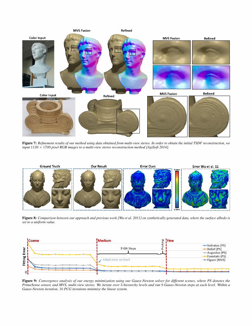
Figure 7: Refinement results of our method using data obtained from multi-view stereo. In order to obtain the initial TSDF reconstruction, weinput 1139× 1709 pixel RGB images to a multi-view stereo reconstruction method [AgiSoft 2014].

Figure 8: Comparison between our approach and previous work [Wu et al. 2011] on synthetically-generated data, where the surface albedo isset to a uniform value.

Figure 9: Convergence analysis of our energy minimization using our Gauss-Newton solver for different scenes, where PS denotes thePrimeSense sensor, and MVS, multi-view stereo. We iterate over 3 hierarchy levels and run 9 Gauss-Newton steps at each level. Within aGauss-Newton iteration, 10 PCG iterations minimize the linear system.

First, we fuse noisy input depth data in order to obtain an initial shaperepresented as a TSDF. While fusion regularizes out noise, it alsoleads to severe over-smoothing, resulting in reconstructions whichlack high-frequency geometric detail. We then run our new shading-based refinement approach directly on the implicit function to obtainthe refined surface geometry along with a spatially-varying albedoestimate for each voxel. Fig. 1 and Fig. 12 show reconstructionresults obtained with a PrimeSense Carmine 1.09 (Short Range)sensor before and after our refinement step. While real-time frame-to-frame tracking suffices for small scenes (i.e., the Augustus (PS)and Sokrates (PS)), we need to perform an offline pose optimizationstep (see Sec. 4.4) for larger scans. All scenes were captured underdifferent uncontrolled lighting conditions. The number of variablesthat need to be optimized during refinement, and the typical amountof iterations used in the refinement optimization are listed in Table1. Effectively, that means we show results with a 0.5mm voxelresolution on the finest level for the fountain scene, and all otherscenes have a 1mm resolution. Note however, that the continuoussigned distance field D provides a higher surface resolution thanthe underlying voxel grid. We compare a refined reconstructionwith a ground truth laser scan in Fig 14. As we can see in thefinal reconstructions, we are able to capture a significant amount ofsurface detail absent from the unrefined result. For instance, note thefine strands in the hair of the Augustus bust, or the fine details andwriting in the Relief. For both weakly and strongly textured objects,our reconstructions are of high accuracy.

In addition to RGB-D scanning, we also show the versatility of ourmethod by using it in a purely image-based reconstruction context.We capture 4 scenes using a multi-view stereo setup, where wereconstruct an initial shape model using a state-of-the-art stereoreconstruction method [AgiSoft 2014]. For each result, 30 imagesare captured with a handheld commodity Canon EOS 1100D cameraand downsampled to 1139×1709 pixels. From the multi-view stereoreconstruction, we obtain a initial TSDF and then run our volumetricshading-based refinement to obtain fine-scale geometric detail. Fig. 7shows the reconstruction results before and after our refinement step.Note that we are able to show significant improvements, even onthese high-quality multi-view stereo reconstructions.

Our method is very stable for different parameter settings; no scene-specific tweaking is needed. There are a few controllable parameters,such as the number of hierarchy levels, or the number of iterationsof the optimizer. These parameters are determined by the differencein input depth and color resolutions; e.g., low-resolution depth andhigh-resolution color will require more hierarchy levels. Results arealso stable on a range of the weights of Erefine; we use a coherent setfor all our results. For input depth with strong noise (this is currentlythe norm for commodity RGB-D data), better results are obtainedwhen using a higher weight for the volumetric regularizer Er .

7.1 Evaluation

We quantitatively evaluate the accuracy of our method onsynthetically-generated depth and color data (see Fig. 8). The datais generated by rendering a mesh from 28 virtual view points with agiven camera trajectory. Through ray casting, we obtain a quantizeddepth map from the ground truth model, and add Gaussian noiseto mimic a real depth sensor’s characteristics. For color data gen-eration, we set the surface reflectance to a uniform value and usethe same spherical harmonics lighting model as in the method of[Ramamoorthi and Hanrahan 2001]. We run our algorithm on thesesimulated depth and RGB images, first obtaining an initial modelby fusing the depth and then applying our shading-based refinementtechnique. The length of the bounding box diagonal of the meshcorresponds to 30cm, and the root-mean-square error is 0.47mm.The error plot on the surface is shown in Fig. 8.

Figure 10: Comparison between our algorithm and Wu et al. [2011]on a multi-view stereo sequence.

Figure 11: Comparison between our approach and Wu et al. [2011]on synthetic data with varying surface albedo.

In addition, we quantitatively compare our method with previouswork, a shading-based refinement method which operates on meshes(MESHRef) [Wu et al. 2011]. As MESHRef requires an input meshinstead of a TSDF, we extract the initial mesh from the implicitfunction. In comparison to our method, MESHRef only obtaineda reconstruction accuracy with root-mean-square error of 0.86mm.Our approach not only improves upon quality, but moreover, sig-nificantly improves computational efficiency. While our methodrequires less than 7.8 seconds, MESHRef takes 20 minutes to ob-tain the refined result. This speedup is largely due to the fact thatminimization of an objective function on a mesh data structure isfundamentally harder than using our hierarchical and sparse gridstructure. In Fig. 11, we provide another comparison on the samedataset, except that we now consider spatially-varying albedo froma painted texture. If we disable albedo optimization – i.e., assume afixed uniform albedo –, we would misinterpret material transitionsas shading cues and hallucinate wrong surface detail; previous workreduce such artifacts by assuming a set of clusters of albedos [Wuet al. 2011], but these artifacts are still very notable. Jointly opti-mizing for both geometric detail and albedo variation with our newchromaticity-based albedo regulizer further mitigates these artifactsand provides a much more realistic solution. We also compare ourmethod with MESHRef on real-world data in Fig. 10. Our approachnot only has a runtime advantage (6.5 seconds against about 1 hour),but also produces higher quality results. Fig. 13 shows a comparisonto the method of [Wu et al. 2014] including a final fusion step. Thisfinal fusion smoothes out some of the previously reconstructed de-tail. In contrast, our approach works in the reverse order and obtainshigher quality results (voxel resolution of 0.5mm in both cases). Thecumulative runtime on the complete sequence is a few seconds forour approach as well as the method of [Wu et al. 2014].

7.2 Runtime and Convergence

We analyze the effectiveness of our method in Fig. 9, which showsconvergence plots for optimizing our objective function. In this eval-uation, we use 3 hierarchy levels and run 9 Gauss-Newton steps on

Seq. Level 3 Level 2 Level 1 Level 0 TotalFuse Opt #Vars Fuse Opt #Vars Fuse Opt #Vars Fuse Opt #Vars #Iter Time

Sokrates (PS) 0.5s 85ms 200k 1.3s 0.1s 520k 1.6s 0.5s 2.0M 1.9s 3.9s 16M 10 9.9sRelief (PS) 0.9s 0.6s 1.2M 1.3s 0.7s 2.5M 1.0s 1.4s 4.0M 1.2s 2.6s 12M 11 9.7s

Augustus (PS) 0.4s 0.1s 200k 1.8s 0.2s 1.5M 2.1s 1.2s 8.5M 2.4s 4.9s 26M 12 13.1sFountain (PS) 0.1s 0.1s 500k 0.2s 0.8s 2.5M 0.3s 1.1s 6.0M 0.5s 2.7s 19M 10 5.8sFigure (MVS) 0.4s 0.8s 600k 1.4s 1.0s 2.7M 2.1s 2.1s 11M 1.9s 2.3s 16M 10 12s

Table 1: Timing measurements for different test scenes, where PS denotes the PrimeSense sensor, and MVS, multi-view stereo.

Figure 12: Refinement results for different scenes captured with a PrimeSense Carmine 1.09 (Short Range) sensor.

Figure 13: The method of Wu et al. [2014] refines independent depth maps, causing detail to smooth out in the subsequent fusion process; i.e.,fuse after refine. Our method refines the geometry after surface fusion, i.e., refine after fuse, thus capturing substantially more detail.

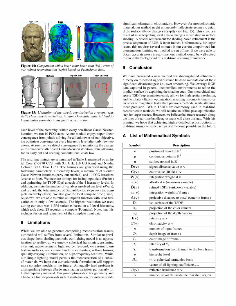
Figure 14: Comparison with a laser scan: laser scan (left), error ofour refined reconstruction (right) based on PrimeSense data.

Figure 15: Limitation of the albedo regularization strategy: spa-tially close albedo variations in monochromatic material lead tohallucinated geometry in the final reconstruction.

each level of the hierarchy; within every non-linear Gauss-Newtoniteration, we run 10 PCG steps. As our method enjoys super-linearconvergence from jointly solving for all unknowns of our objective,the optimizer converges on every hierarchy level after only few iter-ations. At runtime, we detect convergence by monitoring the changein residual error after each Gauss-Newton iteration, thus allowingfor an early out and keeping computational costs low.

The resulting timings are summarized in Table 1, measured on an In-tel Core i7-3770 CPU with 3.4 GHz (16 GB Ram) and NvidiaGeforce GTX Titan GPU. The timings are generated using thefollowing parameters: 4 hierarchy levels, a maximum of 9 outerGauss-Newton iterations (early-out enabled), and 10 PCG iterations(coarse-to-fine). We measure timings for fusing input data (Fusion)and optimizing the TSDF (Opt) at each of the 4 hierarchy levels. Inaddition, we state the number of variables involved per level (#Vars),and provide the total number of Gauss-Newton steps over the com-plete hierarchy (#Iter). We also give the total compute time (Time).As shown, we are able to refine an implicit function with 26M freevariables in only a few seconds. The highest resolution we usedduring our tests was 115M variables based on a 5 level hierarchy,which took about 25 seconds to compute (Fountain). Note, that thisincludes fusion and refinement of the complete input data.

8 Limitations

While we are able to generate compelling reconstruction results,our method still suffers from several limitations. Similar to previ-ous shape-from-shading methods, our lighting model is an approx-imation to reality, as we employ spherical harmonics, assuminga distant, monochromatic light source. Second, we assume Lam-bertian surfaces, and cannot handle specularities, self-occlusions,spatially-varying illumination, or high-frequency textures. Whileour simple lighting model permits the reconstruction of a subsetof materials, we hope that our volumetric formulation will supportmore complex models in the future. An equally hard problem isdistinguishing between albedo and shading variation, particularly forhigh-frequency material. Our joint optimization for geometry andalbedo is a first step towards such disambiguation, for materials with

significant changes in chromaticity. However, for monochromaticmaterial, our method might erroneously hallucinate geometric detailif the surface albedo changes abruptly (see Fig. 15). This error is aresult of misinterpreting local albedo changes as variation in surfaceshading. A crucial requirement for shading-based refinement is theprecise alignment of RGB-D input frames. Unfortunately, for largerscans, this requires several minutes in our current unoptimized im-plementation, limiting our method to run offline. If we were able toobtain accurate poses in real-time, our method would be well-suitedto run in the background of a real-time scanning framework.

9 Conclusion

We have presented a new method for shading-based refinementdirectly on truncated signed distance fields to mitigate one of theirsignificant disadvantages; i.e., over-smoothing. We leverage RGBdata captured in general uncontrolled environments to refine theimplicit surface by exploiting the shading cues. Our hierarchical andsparse TSDF representation easily allows for high spatial resolution,and facilitates efficient optimization, resulting in compute times overan order of magnitude faster than previous methods, while attainingmore precision. While TSDFs are commonly used in real-timereconstruction methods, we still require an offline pose optimizationstep for larger scenes. However, we believe that future research alongthe lines of real-time bundle adjustment will close this gap. With thisin mind, we hope that achieving highly-detailed reconstructions inreal-time using consumer setups will become possible in the future.

A List of Mathematical Symbols

Symbol Description

v position of voxel in R3

p continuous point in R3

n surface normal in R3

D(v) signed distance value at v

C(v) color value (RGB) at v

W(v) integration weight at v

a(v) albedo at v (unknown variable)D(v) refined TSDF (unknown variable)wi(v) integration weight of frame idi(v) projective distance to voxel center in frame iD0 iso-surface of the TSDFπc projection of the color cameraπd projection of the depth camera

I(v) intensity at v

Γ(v) chromaticity at v

n number of input framesDi depth image of frame iCi color image of frame iIi intensity of CiTi transformation from frame i to the base frameq hierarchy levelHm m-th spherical harmonics basisl vector of all lighting coefficients lm

B(v) reflected irradiance at v

N number of voxels inside the thin shell region

Acknowledgements

We would like to thank Qian-Yi Zhou and Vladlen Koltun for theFountain data. This work was funded by the Max Planck Centerfor Visual Computing and Communications, the German ResearchFoundation (DFG), grant GRK-1773 Heterogeneous Image Systems,and the ERC Starting Grant 335545 CapReal. We are grateful for thesupport of a Stanford Graduate Fellowship and gifts from NVIDIACorporation.

References

AGARWAL, S., FURUKAWA, Y., SNAVELY, N., SIMON, I., CUR-LESS, B., SEITZ, S. M., AND SZELISKI, R. 2011. Buildingrome in a day. Communications of the ACM 54, 10, 105–112.

AGISOFT, L. 2014. Agisoft photoscan. Professional Edition.

BEELER, T., BRADLEY, D., ZIMMER, H., AND GROSS, M. 2012.Improved reconstruction of deforming surfaces by cancellingambient occlusion. In Proc. ECCV, 30–43.

BYLOW, E., STURM, J., KERL, C., KAHL, F., AND CREMERS,D. 2013. Real-time camera tracking and 3d reconstruction usingsigned distance functions. In Robotics: Science and Systems(RSS) Conference 2013, vol. 9.

CARR, J. C., BEATSON, R. K., CHERRIE, J. B., MITCHELL, T. J.,FRIGHT, W. R., MCCALLUM, B. C., AND EVANS, T. R. 2001.Reconstruction and representation of 3d objects with radial basisfunctions. In Proc. SIGGRAPH, ACM, 67–76.

CHAN, D., BUISMAN, H., THEOBALT, C., THRUN, S., ET AL.2008. A noise-aware filter for real-time depth upsampling. InWorkshop on Multi-camera and Multi-modal Sensor Fusion Algo-rithms and Applications-M2SFA2 2008.

CHEN, Q., AND KOLTUN, V. 2013. A simple model for intrinsicimage decomposition with depth cues. In The IEEE InternationalConference on Computer Vision (ICCV).

CHEN, J., BAUTEMBACH, D., AND IZADI, S. 2013. Scalablereal-time volumetric surface reconstruction. ACM TOG 32, 4,113.

CUI, Y., SCHUON, S., CHAN, D., THRUN, S., AND THEOBALT, C.2010. 3d shape scanning with a time-of-flight camera. In Proc.CVPR, 1173–1180.

CURLESS, B., AND LEVOY, M. 1996. A volumetric method forbuilding complex models from range images. In Proceedings ofthe 23rd annual conference on Computer graphics and interactivetechniques, ACM, 303–312.

DEBEVEC, P. 2012. The light stages and their applications tophotoreal digital actors. In SIGGRAPH Asia Technical Briefs.

DIEBEL, J., AND THRUN, S. 2006. An application of MarkovRandom Fields to range sensing. 291–298.

DOLSON, J., BAEK, J., PLAGEMANN, C., AND THRUN, S. 2010.Upsampling range data in dynamic environments. In Proc. CVPR,IEEE, 1141–1148.

FUHRMANN, S., AND GOESELE, M. 2014. Floating scale surfacereconstruction. ACM TOG 33, 4, 46.

GHOSH, A., FYFFE, G., TUNWATTANAPONG, B., BUSCH, J., YU,X., AND DEBEVEC, P. 2011. Multiview face capture usingpolarized spherical gradient illumination. ACM TOG 30.

GOLDLUECKE, B., AUBRY, M., KOLEV, K., AND CREMERS, D.2014. A super-resolution framework for high-accuracy multiviewreconstruction. ijcv 106, 2 (jan), 172–191.

HABER, T., FUCHS, C., BEKAER, P., SEIDEL, H.-P., GOESELE,M., AND LENSCH, H. 2009. Relighting objects from imagecollections. In Computer Vision and Pattern Recognition, 2009.CVPR 2009. IEEE Conference on, 627–634.

HAN, Y., LEE, J.-Y., AND KWEON, I. S. 2013. High quality shapefrom a single rgb-d image under uncalibrated natural illumination.In Proc. ICCV.

HASINOFF, S., LEVIN, A., GOODE, P., AND FREEMAN, W. 2011.Diffuse reflectance imaging with astronomical applications. InProc. ICCV, 185–192.

HENRY, P., KRAININ, M., HERBST, E., REN, X., AND FOX, D.2012. RGB-D mapping: Using Kinect-style depth cameras fordense 3D modeling of indoor environments. Int. J. RoboticsResearch 31 (apr), 647–663.

HERNANDEZ, C., VOGIATZIS, G., AND CIPOLLA, R. 2008. Mul-tiview photometric stereo. IEEE PAMI 30, 3, 548–554.

HOPPE, H., DEROSE, T., DUCHAMP, T., MCDONALD, J., ANDSTUETZLE, W. 1992. Surface reconstruction from unorganizedpoints. In Proceedings of the 19th Annual Conference on Com-puter Graphics and Interactive Techniques, ACM, New York, NY,USA, SIGGRAPH ’92, 71–78.

HORN, B. K. 1975. Obtaining shape from shading information.The psychology of computer vision, 115–155.

IZADI, S., KIM, D., HILLIGES, O., MOLYNEAUX, D., NEW-COMBE, R., KOHLI, P., SHOTTON, J., HODGES, S., FREEMAN,D., DAVISON, A., ET AL. 2011. Kinectfusion: real-time 3dreconstruction and interaction using a moving depth camera. InProc. UIST, ACM, 559–568.

KAZHDAN, M., BOLITHO, M., AND HOPPE, H. 2006. Poissonsurface reconstruction. In Proc. SGP.

KEHL, W., NAVAB, N., AND ILIC, S. 2014. Coloured signeddistance fields for full 3d object reconstruction. In Proc. BMVC.

KELLER, M., LEFLOCH, D., LAMBERS, M., IZADI, S., WEYRICH,T., AND KOLB, A. 2013. Real-time 3d reconstruction in dynamicscenes using point-based fusion. In Proc. 3DV, 1–8.

KOPF, J., COHEN, M. F., LISCHINSKI, D., AND UYTTENDAELE,M. 2007. Joint bilateral upsampling. ACM TOG 26, 3.

LEE, K. J., ZHAO, Q., TONG, X., GONG, M., IZADI, S., LEE,S. U., TAN, P., AND LIN, S. 2012. Estimation of intrinsic imagesequences from image+depth video. In Proc. ECCV, 327–340.

LEVOY, M., PULLI, K., CURLESS, B., RUSINKIEWICZ, S.,KOLLER, D., PEREIRA, L., GINZTON, M., ANDERSON, S.,DAVIS, J., GINSBERG, J., SHADE, J., AND FULK, D. 2000.The digital michelangelo project: 3d scanning of large statues. InProc. SIGGRAPH, 131–144.

LINDNER, M., KOLB, A., AND HARTMANN, K. 2007. Data-fusion of PMD-based distance-information and high-resolutionRGB-images. In Proc. ISSCS, 121–124.

LOWE, D. G. 2004. Distinctive image features from scale-invariantkeypoints. IJCV 60, 2, 91–110.

MULLIGAN, J., AND BROLLY, X. 2004. Surface determination byphotometric ranging. In Proc. CVPR Workshops.

NAIR, R., RUHL, K., LENZEN, F., MEISTER, S., SCHAFER, H.,GARBE, C. S., EISEMANN, M., MAGNOR, M., AND KON-DERMANN, D. 2013. A survey on time-of-flight stereo fusion.In Time-of-Flight and Depth Imaging. Sensors, Algorithms, andApplications. Springer, 105–127.

NEHAB, D., RUSINKIEWICZ, S., DAVIS, J., AND RAMAMOORTHI,R. 2005. Efficiently combining positions and normals for precise3D geometry. Proc. SIGGRAPH 24, 3.

NEWCOMBE, R. A., AND DAVISON, A. J. 2010. Live densereconstruction with a single moving camera. In Computer Visionand Pattern Recognition (CVPR), 2010 IEEE Conference on,IEEE, 1498–1505.

NEWCOMBE, R. A., DAVISON, A. J., IZADI, S., KOHLI, P.,HILLIGES, O., SHOTTON, J., MOLYNEAUX, D., HODGES, S.,KIM, D., AND FITZGIBBON, A. 2011. Kinectfusion: Real-timedense surface mapping and tracking. In Proc. ISMAR, IEEE,127–136.

NIESSNER, M., ZOLLHOFER, M., IZADI, S., AND STAMMINGER,M. 2013. Real-time 3d reconstruction at scale using voxelhashing. ACM TOG 32, 6, 169.

PARK, J., KIM, H., TAI, Y.-W., BROWN, M. S., AND KWEON, I.-S. 2011. High quality depth map upsampling for 3d-tof cameras.In Proc. ICCV, IEEE, 1623–1630.

PRADEEP, V., RHEMANN, C., IZADI, S., ZACH, C., BLEYER,M., AND BATHICHE, S. 2013. Monofusion: Real-time 3dreconstruction of small scenes with a single web camera. In Proc.ISMAR.

PRADOS, E., AND FAUGERAS, O. 2005. Shape from shading: awell-posed problem? In Proc. CVPR.

RAMAMOORTHI, R., AND HANRAHAN, P. 2001. A signal-processing framework for inverse rendering. In Proc. SIGGRAPH,ACM, 117–128.

RICHARDT, C., STOLL, C., DODGSON, N. A., SEIDEL, H.-P.,AND THEOBALT, C. 2012. Coherent spatiotemporal filtering,upsampling and rendering of RGBZ videos. CGF (Proceedingsof Eurographics) 31, 2 (May).

ROTH, H., AND VONA, M. 2012. Moving volume kinectfusion. InBMVC, 1–11.

RUSINKIEWICZ, S., HALL-HOLT, O., AND LEVOY, M. 2002.Real-time 3D model acquisition. ACM TOG 21, 3, 438–446.

SCHARSTEIN, D., HIRSCHMULLER, H., KITAJIMA, Y., KRATH-WOHL, G., NESIC, N., WANG, X., AND WESTLING, P. 2014.High-resolution stereo datasets with subpixel-accurate groundtruth. In Pattern Recognition. Springer, 31–42.

SCHUON, S., THEOBALT, C., DAVIS, J., AND THRUN, S. 2009.Lidarboost: Depth superresolution for tof 3d shape scanning. InProc. CVPR, IEEE, 343–350.

SEITZ, S., CURLESS, B., DIEBEL, J., SCHARSTEIN, D., ANDSZELISKI, R. 2006. A comparison and evaluation of multi-viewstereo reconstruction algorithms. In Proc. CVPR, vol. 1, 519–528.

SNAVELY, N., SEITZ, S. M., AND SZELISKI, R. 2006. Phototourism: exploring photo collections in 3d. ACM TOG 25, 3,835–846.

TRIGGS, B., MCLAUCHLAN, P. F., HARTLEY, R. I., AND FITZGIB-BON, A. W. 2000. Bundle adjustment–a modern synthesis. InVision algorithms: theory and practice. Springer, 298–372.

WEBER, D., BENDER, J., SCHNOES, M., STORK, A., AND FELL-NER, D. 2013. Efficient gpu data structures and methods to solvesparse linear systems in dynamics applications. In CGF, vol. 32,Wiley Online Library, 16–26.

WEISE, T., WISMER, T., LEIBE, B., AND VAN GOOL, L. 2009.In-hand scanning with online loop closure. In ICCV Workshops,1630–1637.

WHELAN, T., KAESS, M., FALLON, M., JOHANNSSON, H.,LEONARD, J., AND MCDONALD, J. 2012. Kintinuous: Spatiallyextended kinectfusion.

WU, C., VARANASI, K., LIU, Y., SEIDEL, H.-P., AND THEOBALT,C. 2011. Shading-based dynamic shape refinement from multi-view video under general illumination. In Proc. ICCV, IEEE,1108–1115.

WU, C., STOLL, C., VALGAERTS, L., AND THEOBALT, C. 2013.On-set performance capture of multiple actors with a stereo cam-era. ACM TOG (Proc. SIGGRAPh Asia) 32, 6, 161.

WU, C., ZOLLHOFER, M., NIESSNER, M., STAMMINGER, M.,IZADI, S., AND THEOBALT, C. 2014. Real-time shading-basedrefinement for consumer depth cameras. ACM TOG (Proc. SIG-GRAPH Asia) 33, 6, 200:1–200:10.

YU, L.-F., YEUNG, S.-K., TAI, Y.-W., AND LIN, S. 2013.Shading-based shape refinement of rgb-d images. In Proc. CVPR.

ZHANG, Z., TSA, P.-S., CRYER, J. E., AND SHAH, M. 1999.Shape from shading: A survey. IEEE PAMI 21, 8, 690–706.

ZHOU, Q.-Y., AND KOLTUN, V. 2014. Color map optimization for3d reconstruction with consumer depth cameras. ACM Transac-tions on Graphics (TOG) 33, 4, 155.

ZOLLHOFER, M., NIESSNER, M., IZADI, S., REHMANN, C.,ZACH, C., FISHER, M., WU, C., FITZGIBBON, A., LOOP, C.,THEOBALT, C., ET AL. 2014. Real-time non-rigid reconstructionusing an rgb-d camera. ACM TOG (Proc. SIGGRAPH) 4.