shadows and lights in enzyme kinetics: quasi-steady state
TRANSCRIPT
Shadows and lights in enzyme kinetics:quasi-steady state approximation revisited
Alberto Maria Bersani1 and Guido Dell’Acqua2
1. Dipartimento di Metodi e Modelli Matematici (Me.Mo.Mat.),“La Sapienza” University, Rome, Italy
2. Istituto per le Applicazioni del Calcolo “Mauro Picone” (IAC-CNR),Rome, Italy
Abbreviated Title: Quasi-Steady State Approximation revisited
Corresponding author:Alberto Maria BersaniDipartimento di Metodi e Modelli Matematici (Me.Mo.Mat.)Via A. Scarpa 1600161 Rome, Italy.Tel. +39 0649766681. Fax +39 0649766684e-mail: [email protected]
Abstract
In this paper we re-examine the commonly accepted meaning of thetwo kinetic constants characterizing any enzymatic reaction, accordingto Michaelis-Menten kinetics. Introducing a new asymptotic expansion(in terms of exponentials) of the solutions of the ODEs governing thereaction, we determine a new constant, which corrects some misinter-pretations of current biochemical literature and suggest a new methodto estimate the characteristic parameters of the reaction.
Keywords: Michaelis-Menten kinetics, quasi-steady state approximations,asymptotic expansionsAMS 2000 Subject Classification: 41A58, 41A60, 92C45
1 Introduction
The Michaelis-Menten-Briggs-Haldane approximation, or standard quasi-steady state approximation (sQSSA) [20, 6, 32] represents a milestone in
1
the mathematical modeling of enzymatic reactions.The hypothesis of quasi-steady state is crucial for the interpretation of thereaction and must be handled with much care. It is based on the assump-tion that the complex can be considered ”substantially” constant, but thisstatement has led to many misinterpretations of the model.In fact, as Heineken et al. showed in [13], the exact mathematical interpre-tation of the quasi-steady state assumption is that when we expand asymp-totically the solutions of the ODEs governing the process with respect to anappropriate parameter, the sQSSA is the first order approximation of thesolution.As already observed by Michaelis and Menten by a chemical point of view,this approximation is valid only when the parameter of the expansion issufficiently small. Heineken et al. used the parameter given by the ratioof the initial concentrations of enzyme E and substrate S, obtaining thewell-known chemical requirement.In 1988 Segel [31] and in 1989 Segel and Slemrod [32] obtained the Michaelis-Menten approximation expanding the solutions in terms of a new parameter,including the so-called Michaelis constant and showing that the sQSSA isvalid in a wider range of parameters than the one supposed before.However it is well known that while in vitro the condition on the concentra-tions can be easily fulfilled, in vivo it is not always respected. This meansthat, though very useful, this approximation cannot always be applied.Michaelis-Menten kinetics has recently become very popular thanks to therecent explosion of Systems Biology and in particular of mathematical mod-eling of intracellular enzyme reactions, but in most literature any apriorianalysis of the applicability of sQSSA is absent, even in very complex reac-tion networks. This fact has led to several problems concerning the studyof particular phenomena, like oscillations [10, 25], bistability [8], ultrasensi-tivity [26] or Reverse Engineering [24].Following [17], recent papers [5, 37, 38, 23, 8, 26, 39, 19, 9, 25, 3] have in-troduced and explored a new approximation, called total quasi-steady stateapproximation (tQSSA), which has been shown to be more precise than thesQSSA and to be roughly always valid.Nevertheless, since it is in any case an approximation, also the tQSSA candramatically fail, as shown in [25], but it is doubtless that it is much moreaffordable than the sQSSA.One of the main problems of the mathematical treatment of the sQSSAis the misinterpretation of the hypothesis that the complex time concen-tration has zero derivative. Many papers and even monographies interpretthe ”substantial” equilibrium as a real equilibrium. This is obviously false.Nevertheless much literature uses equations that seem scandalous to anymathematicians ([13], p. 97), obtaining results which are absolutely incon-sistent and false.In this paper we want to re-examine some mathematical aspects of Michaelis-
2
Menten reaction and of the sQSSA, trying to clarify some aspects of theenzyme reactions.The paper is organized in the following way: in Section 2 we recall the mostimportant notions and results on Michaelis-Menten kinetics and sQSSA;in Section 3 we discuss the biochemical and mathematical meaning of thetQSSA, comparing it with the sQSSA; in Section 4 we analyse the conse-quences of the misuse of the sQSSA, reconsidering the meaning of the twokinetic constants Vmax and KM ; in Section 5 we introduce a new expansionin terms of exponentials, which is valid for every choice of the parametersand enzyme initial concentrations; the new expansion is the most appropri-ate to approximate the asymptotic behavior of the solution for large valuesof t; in Section 6 we use the new expansion to solve a serious incoherencepresent in literature, related to the biochemical interpretation of the con-stant KM ; in Section 7, using the expansions introduced in Section 5, wesuggest a new approach to the estimate of the kinetic constants, based onfitting by least squares the experimental data of the time courses of reactantconcentrations.
Finally, let us remark that, due to the stiffness of the system (2), for itsnumerical integration we used a standard stiff MATLAB integrator, ode23s.
2 Notations, definitions and main known results
The model of biochemical reactions was set forth by Henri in 1901 [14, 15, 16]and Michaelis and Menten in 1913 [20] and further developed by Briggs andHaldane in 1925 [6]. This formulation considers a reaction where a substrateS binds an enzyme E reversibly to form a complex C. The complex canthen decay irreversibly to a product P and the enzyme, which is then freeto bind another molecule of the substrate.This process is summarized in the scheme
E + Sa−→←−d
Ck−→ E + P, (1)
where a, d and k are kinetic parameters (supposed constant) associated withthe reaction rates: a is the second order rate constant of enzyme-substrateassociation; d is the rate constant of dissociation of the complex; k is thecatalysis rate constant.Following the mass action principle, which states that the concentrationrates are proportional to the reactant concentrations, the formulation leadsto an ODE for each involved complex and substrate. We refer to this as thefull system.From now on we will indicate with the same symbols the names of theenzymes and their concentrations.The ODEs describing (1) are
3
dSdt = −a(ET − C)S + d C,
dCdt = a(ET − C)S − (d + k)C,
(2)
with initial conditions
S(0) = ST , C(0) = 0, (3)
and conservation laws
E + C = ET , S + C + P = ST . (4)
Here ET is the total enzyme concentration assumed to be free at time t = 0.Also the total substrate concentration, ST , is free at t = 0. This is theso-called Michaelis-Menten (MM) kinetics [20, 4].Let us observe that (2) - (4) admits trivially the asymptotic solution given byC = S = 0, P = ST and E = ET . This means that all the substrate eventu-ally becomes product due to the irreversibility, while the enzyme eventuallyis free and the complex concentration tends to zero.Assuming that the complex concentration is approximately constant aftera short transient phase leads to the usual Michaelis-Menten (MM) approxi-mation, or standard quasi-steady state approximation (sQSSA): we have anODE for the substrate while the complex is assumed to be in a quasi-steadystate (i.e., dC
dt ≈ 0):
C ∼= ET · SKM + S
,dS
dt∼= −kC ∼= − VmaxS
KM + S, S(0) = ST , (5)
where
Vmax = k ET , KM =d + k
a. (6)
KM is the so-called Michaelis constant.The advantage of a quasi-steady state approximation is not only that itreduces the dimensionality of the system, passing from two equations (fullsystem) to one (MM approximation or sQSSA) and thus speeds up numericalsimulations greatly, especially for large networks as found in vivo, but alsothat it allows a theoretical investigation of the system which cannot beobtained with the numerical integration of the full system. Moreover, thekinetic constants in (1) are usually not known, whereas finding the kineticparameters for the MM approximation is a standard in vitro procedure inbiochemistry. See e.g. [4] for a general introduction to this approach. Westress here that this is an approximation to the full system, and that it is only
4
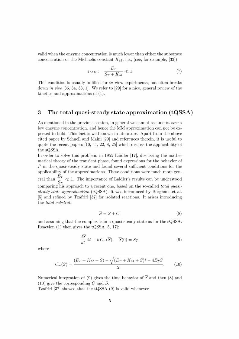
valid when the enzyme concentration is much lower than either the substrateconcentration or the Michaelis constant KM , i.e., (see, for example, [32])
εMM :=ET
ST + KM¿ 1 (7)
This condition is usually fulfilled for in vitro experiments, but often breaksdown in vivo [35, 34, 33, 1]. We refer to [29] for a nice, general review of thekinetics and approximations of (1).
3 The total quasi-steady state approximation (tQSSA)
As mentioned in the previous section, in general we cannot assume in vivo alow enzyme concentration, and hence the MM approximation can not be ex-pected to hold. This fact is well known in literature. Apart from the abovecited paper by Schnell and Maini [29] and references therein, it is useful toquote the recent papers [10, 41, 22, 8, 25] which discuss the applicability ofthe sQSSA.In order to solve this problem, in 1955 Laidler [17], discussing the mathe-matical theory of the transient phase, found expressions for the behavior ofP in the quasi-steady state and found several sufficient conditions for theapplicability of the approximations. These conditions were much more gen-
eral thanET
ST¿ 1. The importance of Laidler’s results can be understood
comparing his approach to a recent one, based on the so-called total quasi-steady state approximation (tQSSA). It was introduced by Borghans et al.[5] and refined by Tzafriri [37] for isolated reactions. It arises introducingthe total substrate
S = S + C, (8)
and assuming that the complex is in a quasi-steady state as for the sQSSA.Reaction (1) then gives the tQSSA [5, 17]:
dS
dt∼= −k C−(S), S(0) = ST , (9)
where
C−(S) =(ET + KM + S)−
√(ET + KM + S)2 − 4ET S
2. (10)
Numerical integration of (9) gives the time behavior of S and then (8) and(10) give the corresponding C and S.Tzafriri [37] showed that the tQSSA (9) is valid whenever
5
εtQSSA :=K
2ST
(ET + KM + ST√
(ET + KM + ST )2 − 4ET ST
− 1
)¿ 1, (11)
(where K =k
a), and that this is at least roughly valid for any sets of
parameters, in the sense that
εtQSSA ≤ K
4KM≤ 1
4. (12)
This means that, for any combination of parameters and initial conditions,(9) is a good approximation to the full system (2). The parameter K isknown as the Van Slyke-Cullen constant. The so-called dissociation constant
KD =d
a[4] is related to the previous kinetic constants by the simple formula
KD = KM −K.Tzafriri [37] expanded equations (10) and (11) in terms of
εTz := r(ST ) :=4ET · ST
(ET + KM + ST )2(13)
and assuming the validity of the tQSSA (εtQSSA ¿ 1) and r ¿ 1, he found
d S
dt∼= −kC−(S) ∼= − VmaxS
KM + ET + S, S(0) = ST , (14)
as a first order approximation to (9). Expression (14) is identical to the for-mula obtained by [5] by means of a two point Pade approximant technique.This approximation is valid at low enzyme concentrations ET ¿ ST + KM ,where it reduces to the MM expression (5), but holds moreover at low sub-strate concentrations ST ¿ ET + KM [37]. Thus, with minimal effort per-forming the substitutions of S by S and of KM by KM + ET , one obtainsa significantly improved MM-like approximation, without any need of moreadvanced mathematics.Moreover Tzafriri found that
εtQSSA =K · ET
(ET + KM + ST )2+ o(r) . (15)
The expressionK · ET
(ET + KM + ST )2appears in the necessary condition, found
by Borghans et al., for the validity of the tQSSA
K · ET
(ET + KM + ST )2¿ 1 (16)
which reduces to the condition given by Laidler for the validity of his ap-proximations, setting S = ST − P .
6
0 1 2 3 4 50
50
100
S
Substrate
t0 1 2 3 4 5
0
50
100
150
200
Sba
r
Substrate + Complex
t
0 1 2 3 4 50
50
100
t
C
Complex
0 1 2 3 4 5−100
0
100
200
t
P
Product
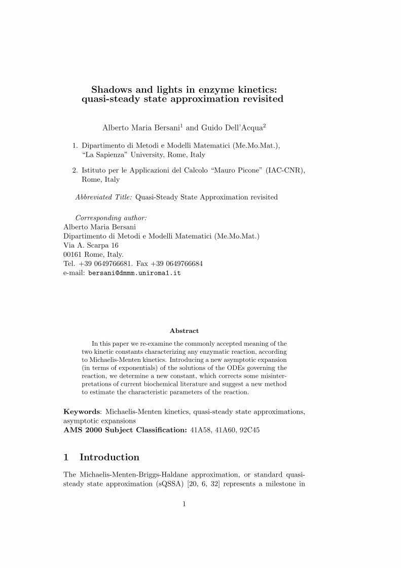
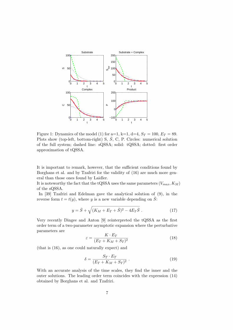
Figure 1: Dynamics of the model (1) for a=1, k=1, d=4, ST = 100, ET = 89.Plots show (top-left, bottom-right) S, S, C, P. Circles: numerical solutionof the full system; dashed line: sQSSA; solid: tQSSA; dotted: first orderapproximation of tQSSA.
It is important to remark, however, that the sufficient conditions found byBorghans et al. and by Tzafriri for the validity of (16) are much more gen-eral than those ones found by Laidler.It is noteworthy the fact that the tQSSA uses the same parameters (Vmax, KM )of the sQSSA.In [39] Tzafriri and Edelman gave the analytical solution of (9), in the
reverse form t = t(y), where y is a new variable depending on S:
y = S +√
(KM + ET + S)2 − 4ET S . (17)
Very recently Dingee and Anton [9] reinterpreted the tQSSA as the firstorder term of a two-parameter asymptotic expansion where the perturbativeparameters are
ε =K · ET
(ET + KM + ST )2(18)
(that is (16), as one could naturally expect) and
δ =ST · ET
(ET + KM + ST )2. (19)
With an accurate analysis of the time scales, they find the inner and theouter solutions. The leading order term coincides with the expression (14)obtained by Borghans et al. and Tzafriri.
7
0 2 4 6 8 100
0.1
0.2
0.3
0.4
0.5
0.6
0.7
S
(A)
0 2 4 6 8 100
0.1
0.2
0.3
0.4
0.5
0.6
0.7
Sbar
v
(B)
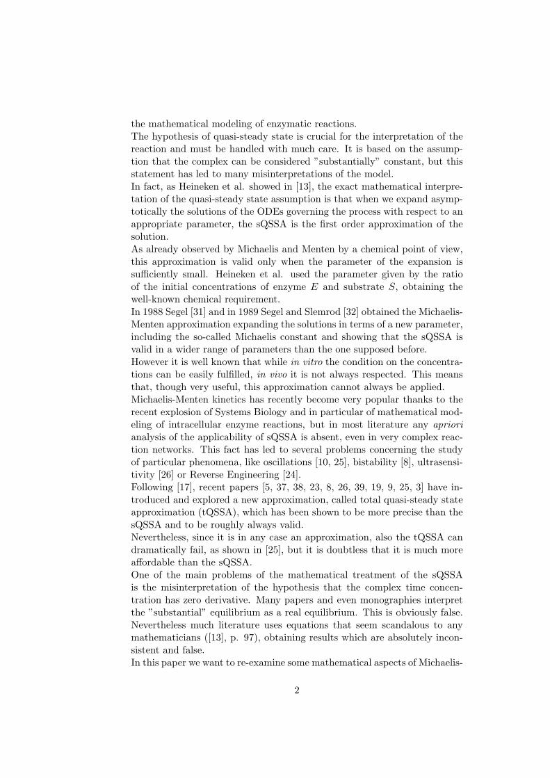
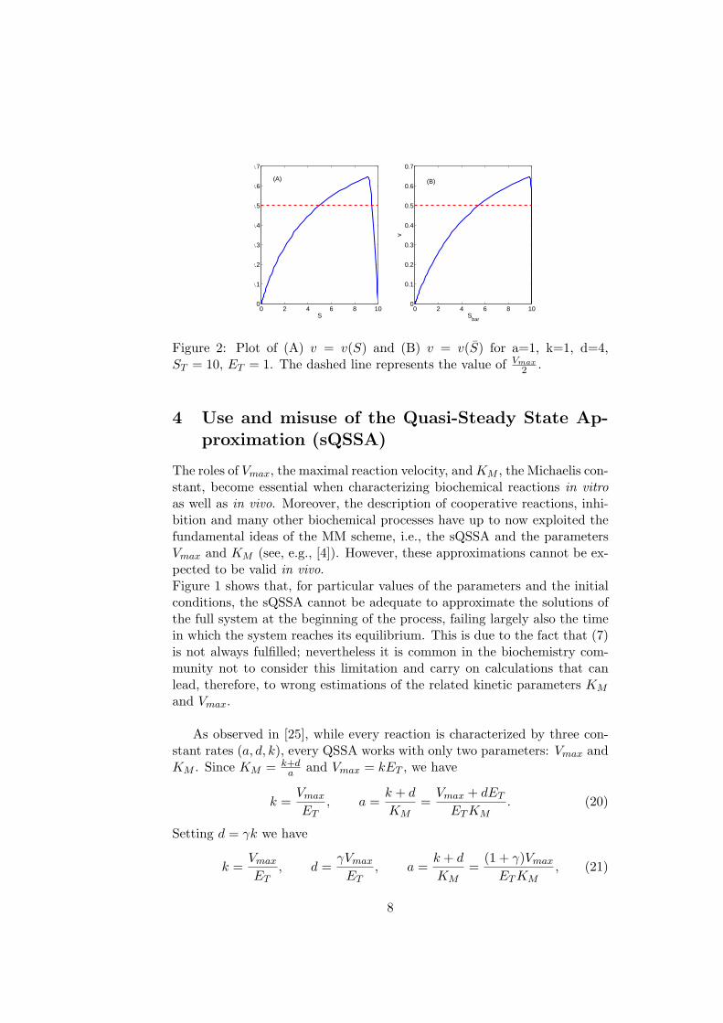
Figure 2: Plot of (A) v = v(S) and (B) v = v(S) for a=1, k=1, d=4,ST = 10, ET = 1. The dashed line represents the value of Vmax
2 .
4 Use and misuse of the Quasi-Steady State Ap-proximation (sQSSA)
The roles of Vmax, the maximal reaction velocity, and KM , the Michaelis con-stant, become essential when characterizing biochemical reactions in vitroas well as in vivo. Moreover, the description of cooperative reactions, inhi-bition and many other biochemical processes have up to now exploited thefundamental ideas of the MM scheme, i.e., the sQSSA and the parametersVmax and KM (see, e.g., [4]). However, these approximations cannot be ex-pected to be valid in vivo.Figure 1 shows that, for particular values of the parameters and the initialconditions, the sQSSA cannot be adequate to approximate the solutions ofthe full system at the beginning of the process, failing largely also the timein which the system reaches its equilibrium. This is due to the fact that (7)is not always fulfilled; nevertheless it is common in the biochemistry com-munity not to consider this limitation and carry on calculations that canlead, therefore, to wrong estimations of the related kinetic parameters KM
and Vmax.
As observed in [25], while every reaction is characterized by three con-stant rates (a, d, k), every QSSA works with only two parameters: Vmax andKM . Since KM = k+d
a and Vmax = kET , we have
k =Vmax
ET, a =
k + d
KM=
Vmax + dET
ET KM. (20)
Setting d = γk we have
k =Vmax
ET, d =
γVmax
ET, a =
k + d
KM=
(1 + γ)Vmax
ET KM, (21)
8
Sf.s. Sf.s. SMM StQSSA STz
a) 4.995 5.045 5 5.05 5εMM
∼= 0.007 εtQSSA∼= 0.0004 εTz
∼= 0.0175errMM
∼= 10−3 errtQSSA∼= 10−3 errTz
∼= 9 · 10−3
b) 4.95 5.45 5 5.5 6εMM
∼= 0.067 εtQSSA∼= 0.004 εTz
∼= 0.156errMM
∼= 10−2 errtQSSA∼= 9 · 10−3 errTz
∼= 0.1c) 0.105 44.6 1 45.5 90
εMM∼= 0.88 εtQSSA
∼= 0.034 εTz∼= 0.99
errMM∼= 8.52 errtQSSA
∼= 2 · 10−2 errTz∼= 1.018
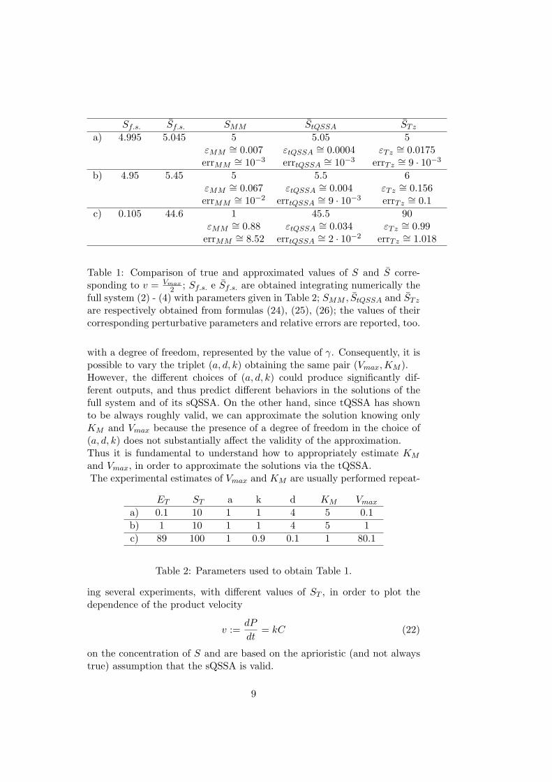
Table 1: Comparison of true and approximated values of S and S corre-sponding to v = Vmax
2 ; Sf.s. e Sf.s. are obtained integrating numerically thefull system (2) - (4) with parameters given in Table 2; SMM , StQSSA and STz
are respectively obtained from formulas (24), (25), (26); the values of theircorresponding perturbative parameters and relative errors are reported, too.
with a degree of freedom, represented by the value of γ. Consequently, it ispossible to vary the triplet (a, d, k) obtaining the same pair (Vmax,KM ).However, the different choices of (a, d, k) could produce significantly dif-ferent outputs, and thus predict different behaviors in the solutions of thefull system and of its sQSSA. On the other hand, since tQSSA has shownto be always roughly valid, we can approximate the solution knowing onlyKM and Vmax because the presence of a degree of freedom in the choice of(a, d, k) does not substantially affect the validity of the approximation.Thus it is fundamental to understand how to appropriately estimate KM
and Vmax, in order to approximate the solutions via the tQSSA.The experimental estimates of Vmax and KM are usually performed repeat-
ET ST a k d KM Vmax
a) 0.1 10 1 1 4 5 0.1b) 1 10 1 1 4 5 1c) 89 100 1 0.9 0.1 1 80.1
Table 2: Parameters used to obtain Table 1.
ing several experiments, with different values of ST , in order to plot thedependence of the product velocity
v :=dP
dt= kC (22)
on the concentration of S and are based on the aprioristic (and not alwaystrue) assumption that the sQSSA is valid.
9
In this case
v = kC ∼= Vmax · SKM + S
. (23)
Consequently Vmax is usually intended as the limit of the ”initial velocity”for the S concentration tending to infinity and KM as the value of S suchthat
v(S = KM ) =Vmax
2. (24)
The values of Vmax and KM are obtained by means of the so-called Lineweaver-Burk plot [4].The so-called ”initial velocity” v must be intended as ”initial velocity afterthe transient phase”. This transient phase is mathematically characterized
by a convex growth of P (during which C, and consequentlydP
dt, grows)
and ends when P graph changes its concavity, i.e., when C, at time tmax,
reaches its maximal value, given by Cmax = C(tmax) =k · ET · S(tmax)KM + S(tmax)
.
ObviouslydC
dt= 0 iff t = tmax.
In the literature we always read that after the transient phase the growthof P is almost linear. But if we recall that the velocity of P is proportionalto the concentration of C and if we look at Figure (1), we easily understandthat C can hardly be considered as “almost constant”; thus by (22) P nevergrows in a linear way. This means that the experimental determination ofthe initial velocity will strongly depend on the time discretization used forthe determination of the slope.In other words the intrinsic bug of using v is strictly connected to the al-
ready discussed problem of stating thatdC
dtis really equal to zero, instead
of being almost equal to zero.Significantly, the original title of Schnell and Maini’s paper [29], as shown onthe web site http://www.cirs-tm.org/researchers/researchers.php?id=694,was ”A century of enzyme kinetics. Should we believe in the Km and vmax
estimates?”. In fact they and some of the authors cited by them criticizethe way used to experimentally compute the parameters.However, the problem of the above mentioned method is not only the lowaccuracy of any estimation of the initial velocity, obtained by means of theslope of a line passing through two different (possibly close each other) pointsof the time course of P just after the transient phase.The problem we want to focus on is not HOW to estimate Vmax or KM ,but IF it is really meaningful to determine the exact behavior of reactantsby means of two parameters which can be determined only through somequasi-steady state approximation.Moreover, we face with the problem that the biochemical interpretation ofKM fails not only when the sQSSA is not valid, but also in many other cases,
10
even when sQSSA holds: for example, when KM > ST . This means that,again, oppositely to what the great majority of biochemistry monographiesreports, definition (24) is not true, in general.Since the tQSSA is much more appropriate than the sQSSA, we can useformula (10) and very simple algebra to define in a more appropriate wayKM (if ST > KM ):
i) when the value of the total substrate is equal to S = KM +ET
2, then
the rate of P is equal toVmax
2:
v
(S = KM +
ET
2
)=
Vmax
2(25)
This result can also be found in [36].
Let us remark, by the way, that if we used Tzafriri approximating formula(14), we would obtain the following definition:
ii) when the value of the total substrate is equal to S = KM + ET , then
the velocity of P is equal toVmax
2:
v(S = KM + ET
)=
Vmax
2(26)
Then the estimate given by (26) becomes largely incorrect for high valuesof ET .Figure (2) shows the behavior of v, as a function of S and S. The graphhas been obtained numerically integrating the full system (2) - (4) and com-puting v by means of formula (22). Let us observe that S is a decreasingfunction of t; thus the phase where C grows from 0 to Cmax corresponds tothe quasi-steady state phase, while the phase where C decreases from Cmax
to 0 corresponds to the transient phase.
We also plotted the horizontal line r of equation v =Vmax
2and determined
the values of S and S corresponding to the intersection of the graph of vwith r, respectively called Sf.s. and Sf.s.. Since the initial velocity is com-puted in the QSS phase, we are interested only in the first intersection.In Tables 1 and 2 we give some examples, where we show the good accuracyof definition (i), even in extremal cases, in contrast with the usual definition(24) and definition (ii): in fact, differently from tQSSA, sQSSA can yieldeven very bad estimates of KM . In Table 1 we report also the relative errors,given by
errMM =|SMM − Sf.s.|
Sf.s.; errtQSSA =
|StQSSA − Sf.s.|Sf.s.
; errTz =|STz − Sf.s.|
Sf.s.
(27)
11
where SMM , StQSSA and STz are respectively given by formulas (24), (25),(26).
5 A new asymptotic expansion for large t
Though the sQSSA is based on the approximationdC
dt∼= 0, several biochem-
istry textbooks (see for example [18, 42, 27, 12]) misuse it, considering theapproximation as a true equality.
As a consequence, the Michaelis constant is determined equating to zerothe right hand side of equation (2) for C, obtaining
KM =E · S
C=
(ET − C) · SC
. (28)
Actually, as shown in Figure (1), the derivative of C is equal to zero only attime t = tmax. Consequently we cannot declare that the right hand side in(28) remains constant.On the other hand, we could interpret KM as the equilibrium value forE · S
C, reached for t tending to infinity, in the same way as the dissociation
constant KD is interpreted in the original Michaelis-Menten reaction, wherek = 0 [27].Actually, while this last reaction, which is completely reversible, reaches asteady-state where both S and C are different from zero, in reaction (1), asabove remarked, S and C tend to zero and consequently we cannot use (28),which gives an undefined ratio, for t →∞.
Thus the equality KM =E · S
Cis valid for every reaction only at t = tmax,
when C reaches its maximum value.We can however try to solve the indetermination of the ratio for t → ∞ inthe following way.From Figure (1) we can observe that, after the transient phase, all the reac-tants seem to follow asymptotically an exponential behavior, with negativeexponent. If we suppose that the asymptotic decay of C is proportional toe−αt, for some α, formula (22) implies that also ST − P will be asymptot-ically proportional to e−αt. By means of the conservation laws (4) we canconclude that also S and ET − E will follow the same asymptotic behavioras C.
Thus let us expand S and C in powers of e−αt: we have
S(t) = S0 + S1 e−αt + S2 e−2αt + o(e−2αt) (29)C(t) = C0 + C1 e−αt + C2 e−2αt + o(e−2αt) (30)
12
0 10 20 30 40
5
10
15
20
25
30
35
40
t
S
(A)
0 10 20 30 400
1
2
3
4
5
6
7
8
tC
(B)
39.1 39.15 39.2 39.25
0.03
0.035
0.04
0.045
0.05
t
S
(C)
39.84 39.85 39.86 39.87
8.84
8.86
8.88
8.9
8.92
8.94
x 10−3
t
C
(D)
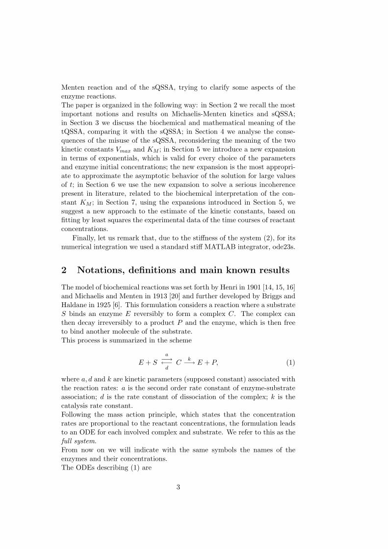
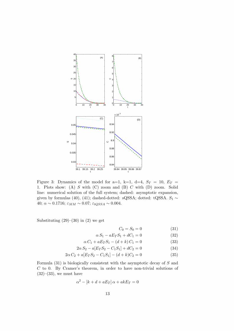
Figure 3: Dynamics of the model for a=1, k=1, d=4, ST = 10, ET =1. Plots show: (A) S with (C) zoom and (B) C with (D) zoom. Solidline: numerical solution of the full system; dashed: asymptotic expansion,given by formulas (40), (41); dashed-dotted: sQSSA; dotted: tQSSA. S1 ∼40; α ∼ 0.1716; εMM ∼ 0.07; εtQSSA ∼ 0.004.
Substituting (29)–(30) in (2) we get
C0 = S0 = 0 (31)α S1 − aET S1 + dC1 = 0 (32)
α C1 + aET S1 − (d + k) C1 = 0 (33)2α S2 − a[ET S2 − C1S1] + dC2 = 0 (34)
2α C2 + a[ET S2 − C1S1]− (d + k)C2 = 0 (35)
Formula (31) is biologically consistent with the asymptotic decay of S andC to 0. By Cramer’s theorem, in order to have non-trivial solutions of(32)–(33), we must have
α2 − [k + d + aET ]α + akET = 0
13
0 50 100 150
5
10
15
20
25
30
35
40
45
50
t
S
(A)
0 50 100 1500
5
10
15
20
25
30
35
40
45
t
C
(B)
142 144 146 148
0
0.005
0.01
0.015
0.02
0.025
0.03
0.035
0.04
0.045
t
S
(C)
140 142 144 146 1480
0.01
0.02
0.03
0.04
0.05
0.06
t
C
(D)
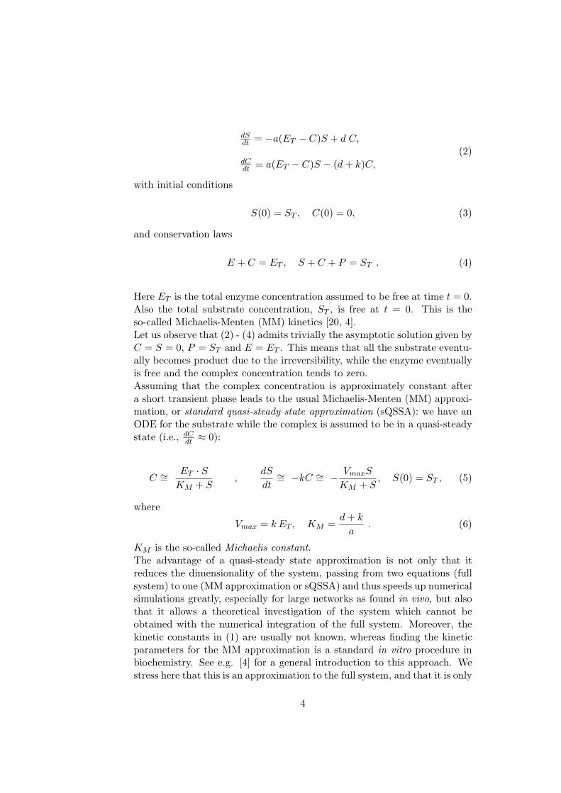
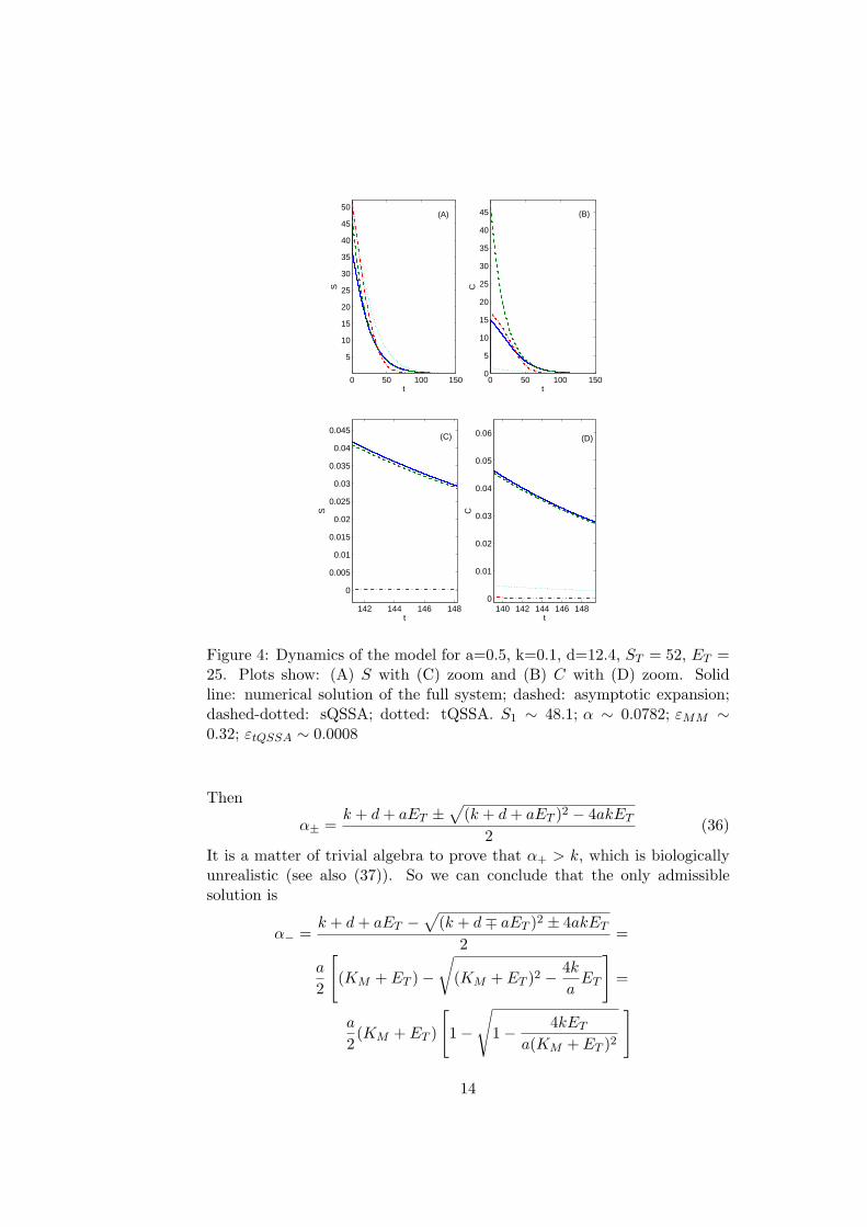
Figure 4: Dynamics of the model for a=0.5, k=0.1, d=12.4, ST = 52, ET =25. Plots show: (A) S with (C) zoom and (B) C with (D) zoom. Solidline: numerical solution of the full system; dashed: asymptotic expansion;dashed-dotted: sQSSA; dotted: tQSSA. S1 ∼ 48.1; α ∼ 0.0782; εMM ∼0.32; εtQSSA ∼ 0.0008
Then
α± =k + d + aET ±
√(k + d + aET )2 − 4akET
2(36)
It is a matter of trivial algebra to prove that α+ > k, which is biologicallyunrealistic (see also (37)). So we can conclude that the only admissiblesolution is
α− =k + d + aET −
√(k + d∓ aET )2 ± 4akET
2=
a
2
[(KM + ET )−
√(KM + ET )2 − 4k
aET
]=
a
2(KM + ET )
[1−
√1− 4kET
a(KM + ET )2
]
14
0 1 2 3 40
20
40
60
80
100
t
S
(A)
0 1 2 3 40
10
20
30
40
50
60
70
80
90
t
C
(B)
3.823 3.824 3.825
0
5
10
15x 10
−3
t
S
(C)
3.76 3.8 3.84 3.88
2.8
3
3.2
3.4
3.6
3.8
4
t
C
(D)
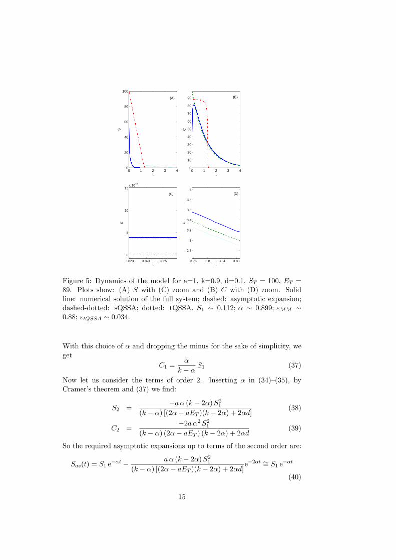
Figure 5: Dynamics of the model for a=1, k=0.9, d=0.1, ST = 100, ET =89. Plots show: (A) S with (C) zoom and (B) C with (D) zoom. Solidline: numerical solution of the full system; dashed: asymptotic expansion;dashed-dotted: sQSSA; dotted: tQSSA. S1 ∼ 0.112; α ∼ 0.899; εMM ∼0.88; εtQSSA ∼ 0.034.
With this choice of α and dropping the minus for the sake of simplicity, weget
C1 =α
k − αS1 (37)
Now let us consider the terms of order 2. Inserting α in (34)–(35), byCramer’s theorem and (37) we find:
S2 =−aα (k − 2α) S2
1
(k − α) [(2α− aET )(k − 2α) + 2αd](38)
C2 =−2aα2 S2
1
(k − α) (2α− aET ) (k − 2α) + 2αd(39)
So the required asymptotic expansions up to terms of the second order are:
Sas(t) = S1 e−αt − aα (k − 2α) S21
(k − α) [(2α− aET )(k − 2α) + 2αd]e−2αt ∼= S1 e−αt
(40)
15
Cas(t) =α
k − αS1 e−αt− 2aα2 S2
1
(k − α) (2α− aET ) (k − 2α) + 2αde−2αt ∼= α
k − αS1 e−αt
(41)
There is still an unknown parameter, S1, which could be estimated fromexperimental data via a least-squares procedure.Figures (3) - (5) compare the time courses of the full system solutions, theirsQSSA and tQSSA and the asymptotic expansions given by (40), (41).In Figure (3) both sQSSA and tQSSA are good approximations, but, asshown in the zoom plots, the asymptotic expansions approximate the solu-tions much better for large t.In Figure (4) the sQSSA begins to fail (εMM
∼= 0.32), while the tQSSAfollows in a very good way the solution. Nevertheless, again the asymptoticexpansion approximates much better the solution for large t.In Figure (5) the sQSSA cannot hold (εMM
∼= 0.88), while the tQSSA stillrepresents a good approximation (εtQSSA
∼= 0.034). Though initially theasymptotic approximation considerably differs from the numerical solution,for large t it represents again the best approximation.As shown in Figures (3) - (5), the estimate of S1 is not related to ST . In par-ticular, in Figure (5) ST = 100 and S1
∼= 0.112. This fact is not in contrastwith our results, because the intent of formulas (40), (41) is to approximatethe solutions for large values of t, no matter what happens for small t.
6 The equilibrium constant revisited
Let us first state the main result of this section.
Theorem 6.1. For t →∞E S
C(t) ∼= Eas Sas
Cas(t) →
(k − α
α
)ET =: KW (42)
Proof. From formulas (40), (41) we get
Sas
Cas(t) =
1− aα(k−2α)S1
(k−α)[(2α−aET )(k−2α)+2αd]e−αt
αk−α
[1− 2a α S1
(2α−aET )(k−2α)+2αde−αt] (43)
When t →∞ we have SasCas
(t) → k−αα . Consequently, since Eas(t) → ET ,
E S
C(t) ∼= Eas Sas
Cas(t) →
(k − α
α
)ET =: KW (44)
16
0 50 100 150 200 250 300
0.1
0.2
0.3
0.4
0.5
0.6
0.7
0.8
0.9
1
t
S*E
/C
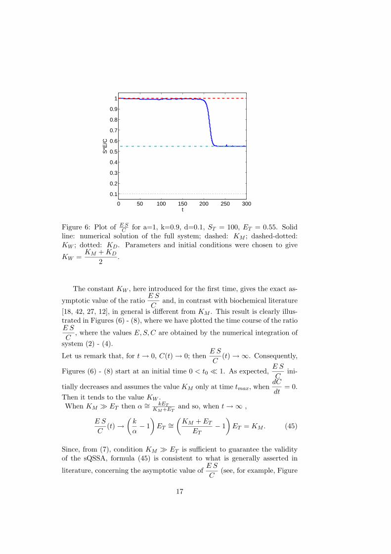
Figure 6: Plot of E SC for a=1, k=0.9, d=0.1, ST = 100, ET = 0.55. Solid
line: numerical solution of the full system; dashed: KM ; dashed-dotted:KW ; dotted: KD. Parameters and initial conditions were chosen to give
KW =KM + KD
2.
The constant KW , here introduced for the first time, gives the exact as-
ymptotic value of the ratioE S
Cand, in contrast with biochemical literature
[18, 42, 27, 12], in general is different from KM . This result is clearly illus-trated in Figures (6) - (8), where we have plotted the time course of the ratioE S
C, where the values E, S,C are obtained by the numerical integration of
system (2) - (4).
Let us remark that, for t → 0, C(t) → 0; thenE S
C(t) →∞. Consequently,
Figures (6) - (8) start at an initial time 0 < t0 ¿ 1. As expected,E S
Cini-
tially decreases and assumes the value KM only at time tmax, whendC
dt= 0.
Then it tends to the value KW .When KM À ET then α ∼= kET
KM+ETand so, when t →∞ ,
E S
C(t) →
(k
α− 1
)ET
∼=(
KM + ET
ET− 1
)ET = KM . (45)
Since, from (7), condition KM À ET is sufficient to guarantee the validityof the sQSSA, formula (45) is consistent to what is generally asserted in
literature, concerning the asymptotic value ofE S
C(see, for example, Figure
17
(7)).
0 1000 2000 3000 4000
0.1
0.2
0.3
0.4
0.5
0.6
0.7
0.8
0.9
1
t
S*E
/C
(A)
2700 2800 2900 3000 3100 3200
0.96
0.965
0.97
0.975
0.98
0.985
0.99
0.995
1
1.005
1.01
tS
*E/C
(B)
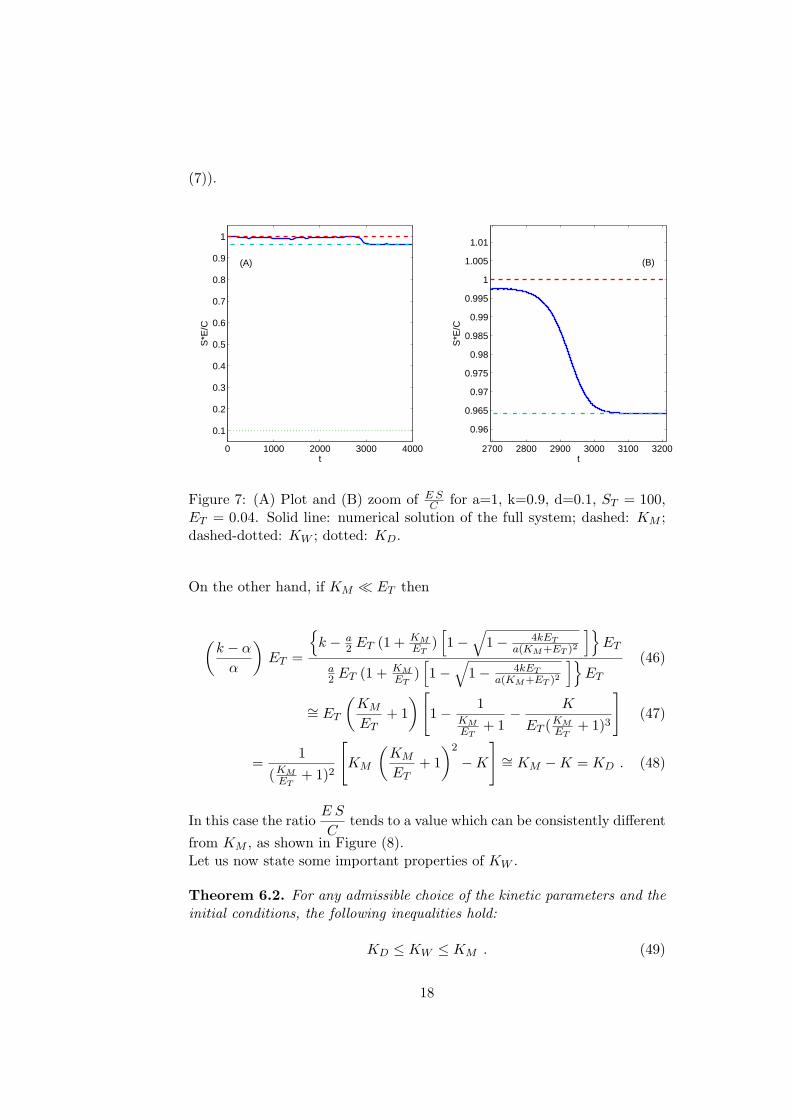
Figure 7: (A) Plot and (B) zoom of E SC for a=1, k=0.9, d=0.1, ST = 100,
ET = 0.04. Solid line: numerical solution of the full system; dashed: KM ;dashed-dotted: KW ; dotted: KD.
On the other hand, if KM ¿ ET then
(k − α
α
)ET =
{k − a
2 ET (1 + KMET
)[1−
√1− 4kET
a(KM+ET )2
]}ET
a2 ET (1 + KM
ET)[1−
√1− 4kET
a(KM+ET )2
]}ET
(46)
∼= ET
(KM
ET+ 1
)[1− 1
KMET
+ 1− K
ET (KMET
+ 1)3
](47)
=1
(KMET
+ 1)2
[KM
(KM
ET+ 1
)2
−K
]∼= KM −K = KD . (48)
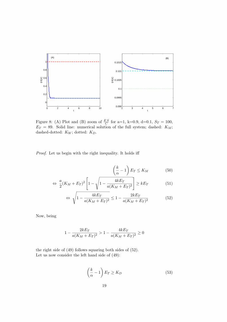
In this case the ratioE S
Ctends to a value which can be consistently different
from KM , as shown in Figure (8).Let us now state some important properties of KW .
Theorem 6.2. For any admissible choice of the kinetic parameters and theinitial conditions, the following inequalities hold:
KD ≤ KW ≤ KM . (49)
18
0 2 4 6 8 10
0
0.2
0.4
0.6
0.8
1
t
S*E
/C
(A)
2 3 4 5 6 70.099
0.0995
0.1
0.1005
0.101
0.1015
tS
*E/C
(B)
Figure 8: (A) Plot and (B) zoom of E SC for a=1, k=0.9, d=0.1, ST = 100,
ET = 89. Solid line: numerical solution of the full system; dashed: KM ;dashed-dotted: KW ; dotted: KD.
Proof. Let us begin with the right inequality. It holds iff
(k
α− 1
)ET ≤ KM (50)
⇔ a
2(KM + ET )2
[1−
√1− 4kET
a(KM + ET )2
]≥ kET (51)
⇔√
1− 4kET
a(KM + ET )2≤ 1− 2kET
a(KM + ET )2(52)
Now, being
1− 2kET
a(KM + ET )2> 1− 4kET
a(KM + ET )2≥ 0
the right side of (49) follows squaring both sides of (52).Let us now consider the left hand side of (49):
(k
α− 1
)ET ≥ KD (53)
19
Being KD = KM − da , (53) holds iff
α
(KM + ET − k
a
)≤ kET
⇔ 1−√
1− 4kET
a(KM + ET )2≤ 2kET
a(KM + ET )(KM + ET − ka)
⇔√
1− 4kET
a(KM + ET )2≥ 1− 2kET
a(KM + ET )(KM + ET − ka)
If the right side of the last inequality is ≤ 0, the proof is over; if this is notthe case, squaring both sides we get
1− 4kET
a(KM + ET )2≥ 1 +
4k2E2T
a2(KM + ET )2(KM + ET − ka)2
− 4kET
a(KM + ET )(KM + ET − ka)
;
⇔(
KM + ET − k
a
)2
+k
aET − (KM + ET )
(KM + ET − k
a
)≤ 0
⇔ −k
a
(KM − k
a
)≤ 0 ⇔ kd ≥ 0
and the proof is over.
Actually, we can say something more: varying appropriately the para-meter values, we can obtain for KW every value between KD and KM . Letus show this fact varying only ET .
Theorem 6.3. For any admissible choice of the kinetic parameters and forany K ∈ (KD , KM ), there exists ET such that ES
C → K when t →∞.
Proof. Let us write
K = βKM + (1− β)KD =d + βk
a(54)
for some β ∈ [0, 1]. Then
(k
α− 1
)ET =
d + βk
a⇔ α =
kET
ET + d+βka
(55)
20
Comparing (55) with the expression of α, we have then
a
2(ET + KM )
(ET +
d + βk
a
)[1−
√1− 4kET
a(KM + ET )2
]= kET
⇔ 1−√
1− 4kET
a(KM + ET )2=
2kET
a(ET + KM )(ET + d+βka )
⇔ 1KM + ET
+kET
a(KM + ET )[KM + ET + k(β−1)
a
]2 −1
KM + ET + k(β−1)a
= 0
⇔ a
[KM + ET +
k(β − 1)a
]2
+ kET − a(ET + KM )[KM + ET +
k(β − 1)a
]= 0
⇔ [a(KM + ET + k(β − 1)](β − 1) + aET = 0
and finally we have
ET =(k + d)(1− β)− k(1− β)2
αβ=
1− β
β
[d + βk
a
]=
1− β
β[βKM + (1− β)KD] .
(56)
Formula (54) justifies the symbol KW : this constant can be seen as aconvex combination of KD and KM , where β is the weight of the combina-tion.Substituting in (56) the expression of β given by (54), we find
ET = KKM − K
K −KD(57)
Moreover, we can express the corresponding α in a simpler way:
α = k (1− β) = a (KM − K) (58)
When β = 0, i.e. K = KD, formula (56) does not hold. In fact, the as-ymptotic value KD is the equilibrium value of the original Michaelis-Mentenreaction, obtained from (1) putting k = 0 [27]. Thus the case β = 0 is bio-logically unrealistic for reaction (1).In any case, we can suppose β ¿ 1 and consequently ET
∼= daβ = KD
β .
Therefore in this case we have ETKD
À 1, that is, ET À KD. In other words,as ET →∞, KW tends to KD, as shown in Figure (8).When β = 1, i.e. K = KM , formula (56) would give ET = 0, which clearlyis not admissible. Let us suppose therefore β = 1− ε with ε ¿ 1. Then weget, at leading order,
ET∼= ε
1− ε
[d + βk
a
]∼= ε(1 + ε)
[d + βk
a
]
∼= ε
[d + k
a
]= εKM
21
Then we have, in this case, ETKM
= ε ¿ 1, that is, ET ¿ KM .These last results are in good agreement with (45) and (48).
7 A new approach to the rate constants estimation
The analysis of the techniques for parameter estimation (inverse problem) isfar beyond the scopes of this paper. We refer to the very interesting paperby Schnell and Maini [29] for an extended discussion of the problem and fora large bibliography. Moreover several authors have recently discussed newapproaches for the experimental determination of the parameter values (seefor example [7, 21, 36, 28, 40, 2] and references therein).Schnell and Mendoza suggest to estimate the parameter values followingthe time course of reactants, fitting the experimental data with the formulaobtained in [30] and based on the Lambert function W , defined by theimplicit formula
W (t)exp [W (t)] = t , (59)
which is the solution of the sQSSA equation (5), instead of repeating severaltimes the same experiment, varying the initial reactant concentrations, inorder to determine the values of the so-called ”initial velocity” v.Their theoretical considerations have been positively experimentally testedby Goudar et al. [11].However the closed formula obtained by Schnell and Mendoza is valid onlyif the sQSSA holds. Otherwise we cannot use it.Making use of the asymptotic approximations introduced in Section 5 (whichare valid for every reaction and every parameter or initial concentrationvalue) and by some simple considerations, we are able to suggest a new wayof estimating the three constant rates a, d, k, starting from the experimentaldata of the time courses of S, E, C and P .Let us first observe that in literature it is usually declared that at the be-ginning, mainly when the initial substrate concentration ST is high, we canaffirm that S remains constant.Actually, when we determine from (2) the initial rates of the concentrations,we have
dS
dt(0) =
dE
dt(0) = −dC
dt(0) = −aET ST ;
dP
dt(0) = 0 . (60)
Then the mathematical model says that, for increasing values of ST ,∣∣∣dS
dt(0)
∣∣∣grows, while the ratio
dSdt (0)ST
= −aET (61)
22
does not depend on ST .
On the other hand, when we use the tQSSA, we havedS
dt= −kC and
consequentlydS
dt(0) = 0.
This means that during the transient phase we cannot suppose that S isapproximately constant, but we can reasonably suppose S ∼= ST , as correctlyset for the inner solutions, for t < tmax, in the tQSSA asymptotic expansions[17, 5, 37, 9].
i) estimate of aEquations (60) give a way to determine experimentally the parameter a,starting from the experimental data at the very beginning of the reaction:given t1 and t2, such that t1, t2 ¿ 1,
a ∼= 1ET ST
[S(t1)− S(t2)
t2 − t1
]∼= 1
ET ST
[E(t1)−E(t2)
t2 − t1
]∼= 1
ET ST
[C(t2)− C(t1)
t2 − t1
].
(62)The advantage of this estimate is given by the fact that, in the same exper-iment, the value of a can be determined in three different ways at the sametwo times t1 and t2.The other parameters can be estimated by means of formula (42), using theexperimental data of C, S and E for t sufficiently large.
ii) estimate of dPerforming an experiment with a very high initial concentration of ET
(ET →∞) and for sufficiently large values of t,
KD =d
a∼= S(t)E(t)
C(t)=
S(t) [ET − C(t)]C(t)
(63)
thus, knowing a from (62), we have
d = aKD∼= a ·
[S(t)E(t)
C(t)
]. (64)
In this case we can test the validity of KD (and a) estimates computing the
ratioS(t)E(t)
C(t)at different (sufficiently large) times.
iii) estimate of kThe case ET À 1 (β ¿ 1) can be used also for the estimate of k: in fact, inthis case, from formula (58), α ∼= k.Thus, fitting the experimental data of S with formula (40), we can estimateboth S1 and α and thus k, too.
On the other hand, since, for ET → 0,SE
C→ KW
∼= KM for t →∞, we can
perform experiments with ET ¿ 1, estimating KM (and thus k = aKM −d)
by means of the values ofSE
C(t) for t sufficiently large.
23
Though the approach here proposed needs the replication of experimentswith different values of ET (in particular ET À 1 and ET ¿ 1), it has theadvantage that it can directly estimate the three kinetic parameters a, d, kand that for every experiment the same estimate can be repeated for severalvalues of t, using the experimental time course of the concentrations.
Acknowledgements
G. D. acknowledges support by the EC, contract “FP6-2005-NEST-PATH,No. 043241 (ComplexDis)”.
References
[1] K. R. Albe, M. H. Butler and B. E. Wright, Cellular Concen-tration of Enzymes and Their Substrates, J. Theor. Biol., 143 (1990),pp. 163–195.
[2] R. A. Alberty, Determination of kinetic parameters of enzyme-catalyzed reactions with a minimum number of velocity measurements,J. Theor. Biol., 254 (2008), pp. 156–163.
[3] D. Barik, M. R. Paul, W. T. Baumann, Y. Cao andJ. J. Tyson, Stochastic Simulation of Enzyme-Catalized Reactionswith Disparate Time Scales, to appear on Biophys. J.
[4] H. Bisswanger, Enzyme Kinetics. Principles and Methods, Wiley-VCH, (2002).
[5] J. Borghans, R. de Boer and L. Segel, Extending the quasi-steady state approximation by changing variables, Bull. Math. Biol.,58 (1996), pp. 43–63.
[6] G. E. Briggs and J. B. S. Haldane, A note on the kinetics ofenzyme action, Biochem. J., 19 (1925), pp. 338–339.
[7] K.-H. Cho, S.-Y. Shin, H. W. Kim, O. Wolkenhauer, B. Mc-Ferran and W. Kolch, Mathematical Modeling of the Influence ofRKIP on the ERK Signaling Pathway, Computational Methods in Sys-tems Biology, First International Workshop, CMSB 2003, Rovereto,Italy, February 24-26, 2003, Proceedings, Corrado Priami (Ed.), Lec-ture Notes in Computer Science 2602 Springer (2003).
[8] A. Ciliberto, F. Capuani and J. J. Tyson, Modeling networks ofcoupled anzymatic reactions using the total quasi-steady state approx-imation, PLoS Comput. Biol., 3 (2007), pp. 463–472.
24
[9] J. W. Dingee and A. B. Anton, A New Perturbation Solution tothe Michaelis-Menten Problem, AIChE J., 54 (2008), pp. 1344–1357.
[10] E. H. Flach and S. Schnell, Use and abuse of the quasi-steady-state approximation, IEE Proc.-Syst. Biol., 153 (2006), pp. 187–191.
[11] C. T. Goudar, S. K. Harris, M. J. McInerney and J. M. Su-flita, Progress curve analysis for enzyme anf microbial kinetic re-actions using explicit solutions based on the Lambert W function, J.Microbiol. Meth., 59 (2004), pp. 317–326.
[12] G. G. Hammes, Thermodynamics and kinetics for the biological sci-ences, Wiley-Interscience, (2000).
[13] F. G. Heineken, H. M. Tsushiya and R. Aris, On the Mathe-matical Status of the Pseudo-steady State Hypothesis of BiochemicalKinetics, Math. Biosc., 1 (1967), pp. 95–113.
[14] V. Henri, Recherches sur la loi de l’action de la sucrase, C. R. Hebd.Acad. Sci., 133 (1901), pp. 891–899.
[15] V. Henri, Uber das Gesetz der Wirkung des Invertins, Z. Phys.Chem., 39 (1901), pp. 194–216.
[16] V. Henri, Theorie generale de l’action de quelques diastases, C. R.Hebd. Acad. Sci., 135 (1902), pp. 916–919.
[17] K. J. Laidler, Theory of the transient phase in kinetics, with specialreference to enzyme systems, Can. J. Chem., 33 (1955), pp. 1614–1624.
[18] A. L. Lehninger, Biochimica, Zanichelli, (1979), italian translationfrom Biochemistry, Worth Publ., (1975).
[19] S. MacNamara, A. M. Bersani, K. Burrage and R. B. Sidje,Stochastic chemical kinetics and the total quasi-steady-state assump-tion: application to the stochastic simulation algorithm and chemicalmaster equation, Preprint Me.Mo.Mat. n. 3/2007, to appear on J.Chem. Phys.
[20] L. Michaelis and M. L. Menten, Die kinetik der invertinwirkung,Biochem. Z., 49 (1913), pp. 333–369.
[21] C. G. Moles, P. Mendes and J. R. Banga, Parameter Estima-tion in Biochemical Pathways: A Comparison of Global OptimizationMethods, Genome Res., 13 (2003), pp. 2467–2474.
[22] L. Noethen and S. Walcher, Quasi-steady state in Michaelis-Menten system, Nonlinear Anal., 8 (2007), pp. 1512–1535.
25
[23] M. G. Pedersen, A. M. Bersani and E. Bersani, The Total QuasiSteady-State Approximation for Fully Competitive Enzyme Reactions,Bull. Math. Biol., 69 (2005), pp. 433–457.
[24] M. G. Pedersen, A. M. Bersani, E. Bersani and G. Cortese,The Total Quasi-Steady State Approximation for Complex Enzyme Re-actions, Proceedings 5th MATHMOD Conference, ARGESIM Reportn. 30, Vienna University of Technology Press (2006), to appear inMathematics and Computers in Simulation.
[25] M. G. Pedersen, A. M. Bersani and E. Bersani, Quasi Steady-State Approximations in Intracellular Signal Transduction – a Wordof Caution, J. Math. Chem., 43 (2008), pp. 1318–1344.
[26] M. G. Pedersen and A. M. Bersani, The Total Quasi-Steady StateApproximation Simplifies Theoretical Analysis at Non-Negligible En-zyme Concentrations: Pseudo First-Order Kinetics and the Loss ofZero-Order Ultrasensitivity, Preprint Me.Mo.Mat. n. 4/2007, submit-ted to Biophys. Chem.
[27] N. C. Price and L. Stevens, Fundamentals of Enzymology, OxfordUniv. Press, (1989).
[28] M. Rodriguez-Fernandez, P. Mendes and J. R. Banga, A hy-brid approach for efficient and robust parameter estimation in bio-chemical pathways, Biosystems, 83 (2006), pp. 248–265.
[29] S. Schnell and P. K. Maini, A century of enzyme kinetics. Re-liability of the KM and vmax estimates, Comments Theor. Biol., 8(2003), pp. 169–187.
[30] S. Schnell and C. Mendoza, A closed-form solution for time-dependent enzyme kinetic, Journal of theoretical Biology, 187 (1997),pp. 207–212.
[31] L. A. Segel, On the validity of the steady-state assumption of enzymekinetics. Bull. Math. Biol., 50 (1988), pp. 579–593.
[32] L. A. Segel and M. Slemrod, The quasi steady-state assumption:a case study in pertubation, SIAM Rev., 31 (1989), pp. 446–477.
[33] A. Sols and R. Marco, Concentrations of metabolites and bindingsites, Implications in metabolic regulation, Curr. Top. Cell. Regul., 2eds. B. Horecker and E. Stadtman (1970), pp. 227–273.
[34] P. A. Srere, Enzyme Concentrations in Tissues, Science, 158 (1967),pp. 936–937.
26
[35] O. H. Straus and A. Goldstein, Zone Behavior of Enzymes, J.Gen. Physiol., 26 (1943), pp. 559–585.
[36] P. Toti, A. Petri, V. Pelaia, A. M. Osman, M. Paoloni andC. Bauer, A linearization method for low catalytic activity enzymekinetic analysis, Biophys. Chem., 114 (2005), pp. 245–251.
[37] A. R. Tzafriri, Michaelis-Menten kinetics at high enzyme concen-trations, Bull. Math. Biol., 65 (2003), pp. 1111–1129.
[38] A. R. Tzafriri and E. R. Edelman, The total quasi-steady-stateapproximation is valid for reversible enzyme kinetics, J. Theor. Biol.,226 (2004), pp. 303–313.
[39] A. R. Tzafriri and E. R. Edelman, Quasi-steady-state kinetics atenzyme and substrate concentrations in excess of the Michaelis-Mentenconstant, J. Theor. Biol., 245 (2007), pp. 737–748.
[40] R. Varon, M. Garcia-Moreno, J. Masia-Perez, F. Garcıa-Molina, F. Garcıa-Canovas, E. Arias, E. Arribas andF. Garcıa-Sevilla, An alternative analysis of enzyme systems basedon the whole reaction time: evaluation of teh kinetic parameters andinitial enzyme concentration, J. Math. Chem., 42 (2007), pp. 789–813.
[41] N. G. Walter, Michaelis-Menten is dead, long live Michaelis-Menten!, Nat. Chem. Biol., 2 (2006), pp. 66–67.
[42] E. N. Yeremin, The foundations of chemical kinetics, MIR Pub.,(1979).
27