shakti ranjan garanayak - ethesisethesis.nitrkl.ac.in/4733/1/211me2348.pdf · a thesis submitted in...

A thesis Submitted in partial fulfilment of the requirements for

the award of the degree of

Master of Technology

In

Mechanical Engineering

(Production Engineering)

By

Shakti Ranjan Garanayak (211ME2348)

Under The Guidance of

Prof. K. P. Maity

Department of Mechanical Engineering

National Institute of Technology Rourkela

Orissa -769008, India

May 2013

A thesis Submitted in partial fulfilment of the requirements for

the award of the degree of

Master of Technology

In

Mechanical Engineering

(Production Engineering)

By

Shakti Ranjan Garanayak

(211ME2348) Under the guidance of

Prof. K. P. Maity


National Institute of Technology Rourkela

Orissa -769008, India

May 2013

National Institute of Technology

Rourkela

CERTIFICATE

This is to certify that the thesis entitled ― CFD analysis and Optimization of

Abrasive Flow Machining submitted to the National Institute of Technology,

Rourkela (Deemed University) by Shakti Ranjan Garanayak Roll No.

211ME2348 for the award of the Degree of Master of Technology in

Mechanical Engineering with specialization in―Production Engineering is a

record of bonafide research work carried out by him under my supervision and

guidance. The results presented in this thesis has not been, to the best of my

knowledge, submitted to any other University or Institute for the award of any

degree or diploma. The thesis, in my opinion, has reached the standards

fulfilling the requirement for the award of the degree of Master of technology in

accordance with regulations of the Institute.

Place: Rourkela Dr. K. P. Maity

Date Professor


National Institute of Technology, Rourkela

DEDICATED TO

MY DEAREST

JHUMI

ii

Acknowledgement

I express my deep sense of gratitude and indebtedness to my thesis

supervisor Dr. K. P. Maity, Professor and Head on Department of Mechanical

Engineering for providing precious guidance, inspiring discussions and constant

supervision throughout the course of this work. His timely help, constructive

criticism, and conscientious efforts made it possible to present the work

contained in this thesis.

I express my sincere thanks to Mr. Alok Ranjan Biswal, Ph.D scholar

and Dillip Bagal, Research Scholar and Mr. Abhijeet Majumdar, Technical

Assistant in Production Engineering lab, for their support during the project

work. I am also thankful to all the staff members of the department of

Mechanical Engineering and to all my well-wishers for their inspiration and

help. I am also thankful to my classmates Ved Prakash Kishor, Poorna chandu

karuturi, Debasis Nayak , Neelam Verma for their help during my project work.

I feel pleased and privileged to fulfil my parent’s ambition and I am

greatly indebted to them for bearing the inconvenience during my M Tech.

course.

Date Shakti Ranjan Garanayak

Roll No - 211ME2348

ABSTRACT

This study deals with a new approach to understand the micro finishing of abrasive

flow machining process in which computational fluid dynamics is used to simulate the forces.

Mathematical modelling is applied to model the micro finishing operation. The study is

conducted to compare the simulated results with the existing experimental results. A flexible

polishing tool comprising polishing medium is used to carry out the analysis. The relative

motion between the polishing medium and the workpiece surface provides the required

finishing action. In the present work a two dimensional computational fluid dynamics

simulation inside the workpiece fixture is performed to evaluate the axial and radial stresses

developed due to the flow of polishing medium. The present study also develops optimization

for AFM process of Al. alloy using response surface method. It is found that all the three

machining parameters and some of their interactions have significant effect on outputs

considered in the present study. Finally, an attempt has been made to estimate the optimum

machining conditions to produce the best possible output within the experimental constraints.

Keywords: AFM, Simulation, RSM, ANOVA

iv | P a g e

Contents

Sl.No. Contents Page No.

Certificate i

Acknowledgement ii

Abstract iii

Contents iv

List of Figures viii

List of Tables xi

1 Introduction

1.1 Overview Of Traditional Finishing Process 1

1.2 Advance Abrasive Finishing Process 2

1.2.1 Magnetic Abrasive Finishing Process 3

1.2.2 Magneto Rheological Finishing Process 3

1.2.3 Magneto Rheological Flow Polishing Process 4

1.3 Limitation Of Magnetic Field Assisted Finishing

Processes

5

1.4 Abrasive Flow Machining Process (AFM) 5

1.4.1 Working Principle 6

1.4.2 Abrasive Flow Machining System 7

1.4.3 Features of AFM 7

1.4.4 Application of AFM 8

2 Literature Reviews 10

2.1 AFM Process Mechanism 10

2.2 Surface Finish And Material Removal

Mechanism:

11

2.3 Medium Composition And Its Rheology 12

2.4 Active Grains 13

2.5 Force And Specific Energy 13

2.6 Representation Of Surface Roughness 14

2.7 Recent Advances on AFM Processes 14

2.7.1 Magnetic AFM Process 14

v | P a g e

2.7.2 Electro-Chemically Assisted Abrasive Flow

Machining Process

14

2.7.3 Ultrasonic Flow Polishing 15

2.7.4 Spiral Polishing 15

2.7.5 Centrifugal Force Assisted Abrasive Flow

Machining Process

15

2.7.6 Drill-bit guided Abrasive flow finishing process 15

2.8 Limitation of AFM 16

2.9 Objective Of The Present Work 16

3 Simulation Of AFM 17

3.1 Computational Fluid Dynamics (CFD): 17

3.1.1 Discretization Method 19

3.1.1.1 Finite Volume Method (FVM) 19

3.1.1.2 Finite Element Method (FEM) 19

3.1.1.3 Finite Difference Method 20

3.1.2 How Does CFD Work 20

3.1.2.1 Pre-Processing 20

3.1.2.2 Solver 21

3.1.2.3 Post-Processing 21

3.1.3.1 Present Study 21

3.1.3.2 Governing Equations 22

3.1.3.3 Geometry Of Workpiece 23

3.1.3.4 Geometry Of Workpiece with fixture 23

3.1.3.5 Design Of Work Piece With Fixture In Gambit 23

3.1.3.6 Meshed diagram Of Work Piece With Fixture 24

3.1.3.7 Parameter Setting 25

3.1.6.8 Boundary Conditions 25

3.1.3.9 Numerical Method 25

3.1.4.1 Steps Of Fluent Analysis 26

3.1.5.1 Modelling Of Material Removal 27

3.2 Simulation On A Cylindrical Pipe 31

3.2.1 Simulation Through CFD (Fluent: ANSYS 13) 31

4 Result and Discussion 32

vi | P a g e

4.1 Result And Discussion for flat work-piece 32

4.1.1 Velocity Distribution 32

4.1.2 Plot Of Velocity Magnitude With Position 33

4.1.3 Distribution Of Velocity Vector 33

4.1.4 Pressure Distribution 34

4.1.5 Plot Of Static Pressure With Position 35

4.1.6 Strain Distribution 35

4.1.7 Plot Of Strain Rate With Position 36

4.1.8 Plot Of Axial Wall Shear Stress With Position 37

4.1.9 Plot Of Radial Wall Shear Stress With Position 37

4.2 Results And Discussion Of Flow Inside A Pipe 39

4.2.1 Velocity Distribution 39

4.2.2 Plot Of Velocity Magnitude With Position 39

4.2.3 Pressure Distribution 40

4.2.4 Plot Of Variation Of Pressure In Axial Direction 40

4.2.5 Plot Of Axial Wall Shear Stress 41

4.2.6 Plot Of Radial Wall Shear Stress 41

5 Optimization 43

5.1 Response Surface Methodology 43

5.1.1 Optimization Techniques 45

5.1.2 Test For Significance Of The Regression Model 45

5.1.3 Test For Significance On Individual Model

Coefficients

45

5.1.4 Test For Lack-Of-Fit 46

5.2 Results And Discussion 46

5.2.1 Residual Plots 56

5.2.2 Contour Plots 59

6 Conclusion 64

7 References 65

viii | P a g e

LIST OF FIGURES

Figure no. Title Page no.

1. Magnetic abrasive flow machining …. ……………………………….. 3

2. Magnetic Rheological finishing ……………………………………... 3

3. Magneto rheological flow polishing…………………………………… 4

4. Abrasive Flow machining ………………………………………….. 5

5. Schematic diagram of AFM ………………………………………… 6

6. Surface finish of various components…………………………………… 8

7. AFM of some complex holes …………………………………………. 8

8. AFM of complex cylindrical holes …………………………………… 9

9. Tooling for AFM …………………………………………………. 9

10. Shows the workpiece with dimension ………………………………… 23

11. Shows the workpiece fixture ………………………………………... 23

12. Geometry of workpiece with fixture…………………………………... 23

13. Meshed diagram of workpiece with fixture…………………………… 24

14. Forces acting during AFM ……………………………………….. 27

15. Mechanism of material removal …………………………………… 28

16. Mechanism with forces during AFM………………………………… 28

17. The modelling and meshing of pipe…………………………………….. 31

18. Velocity distribution ……………………………………………… 32

19. Velocity distribution on full view of work piece ………………………….. 32

20. Velocity magnitude with position ……………………………………… 33

21. Distribution of velocity vector …………………………………………… 33

22. Pressure distribution ……………………………………………...... 34

23. Pressure distribution of full view of work piece ………………………… 34

24. Static pressure with position……………………………………...... 35

25. Strain distribution ………………………………………………..... 35

26. Strain distribution of full view of work piece……………………………. 36

27. Strain rate with position …………………………………………….. 36

28. Axial wall shear stress with position ………………………………….. 37

ix | P a g e

29. Radial wall shear stress with position …………………………... 37

30. Velocity distribution …………………………………………. 39

31. Velocity magnitude with in radial direction………………………… 39

32. Pressure distribution………………………………………... 40

33. Static pressure with position …………………………………. 40

34. Axial wall shear stress with position……………………………… 41

35. Radial wall shear stress with position……………………………… 41

36. Normal probability plot of axial stress……………………………. 56

37. Versus fit for axial stress …………………………………. 56

38. Histogram of axial stress………………………………………… 56

39. Versus order for axial stress …………………………………….. 56

40. Normal probability plot of radial stress …………………………... 57

41. Versus fit for radial stress …………………………………… 57

42. Histogram of radial stress……………………………………….. 57

43. Versus order of radial stress …………………………………… 57

44. Normal probability plot of indentation depth ………………………... 58

45. Versus fit for indentation depth ………………………………... 58

46. Histogram of indentation depth ……………………………………... 58

47. Versus order of indentation depth ………………………………… 58

48. 3D contour plot of axial stress vs. vol.fraction, pressure ……………. 59

49. 2D contour plot of axial stress vs. vol. fraction, pressure………………….59

x | P a g e

50. 3D contour plot of axial stress vs. vol.fraction, velocity………………….. 59

51. 2D contour plot of axial stress vs. vol. fraction, velocity…………………..59

52. 3D contour plot of axial stress vs. pressure, velocity……………………....60

53. 2D contour plot of axial stress vs. pressure, velocity………………………60

54. 3D contour plot of radial stress vs. vol.fraction, pressure………………… 60

55. 2D contour plot of radial stress vs. vol.fraction, pressure………………… 60

56. 3D contour plot of radial stress vs. vol.fraction, velocity………………… 61

57. 2D contour plot of radial stress vs. vol.fraction, velocity………………… 61

58. 3D contour plot of axial stress vs. pressure, velocity …………………… 61

59. 2D contour plot of axial stress vs. pressure, velocity………………………61

60. 3D contour plot of indentation depth vs. vol.fraction, pressure…………. 62

61. 2D contour plot of indentation depth vs. vol.fraction, pressure…………. 62

62. 3D contour plot of indentation depth vs. vol.fraction, velocity ……………62

63. 3D contour plot of indentation depth vs. vol.fraction, velocity………….. 62

64. 3D contour plot of indentation depth vs. pressure, velocity…………… 63

65. 2D contour plot of indentation depth vs. pressure, velocity……………… 63

xi | P a g e

LIST OF TABLES

Table no. Title Page no.

1. Value of Input Process Parameters 47

2. Design Table Randomized 47

3. Design table 48

4. Value of Output responses 49

5. Estimated Regression Coefficients for AXIAL STRESS 50

6. Analysis of Variance for AXIAL STRESS 51

7. Estimated Regression Coefficients for RADIAL STRESS 52

8. Analysis of Variance for RADIAL STRESS 53

9. Estimated Regression Coefficients for INDENTATION DEPTH 54

10. Analysis of Variance for INDENTATION DEPTH 55

1 | P a g e

Chapter 1

Introduction of AFM

Precision and Ultra finishing process represents a critical and expensive phase of the

overall production process. Manufacturing of precision parts consists a stage of final

finishing operation. It is mostly uncontrollable, labour intensive and frequently involves a

reasonable part of the total manufacturing cost. The functional properties such as wear

resistance and power loss due to friction are influenced by surface roughness of the matching

parts [1, 3].

To counter the problems such as high direct labour cost and to produce finished

precision parts with specific features for finishing inaccessible areas, abrasive finishing

techniques are developed. Abrasive finishing process is carried with large number of cutting

edges which have indefinite orientation and geometry. Abrasive fine process are commonly

employed due to their capacity of finishing various geometries of form (i.e. Flat, round etc.)

with desired dimensional accuracies and surface finish [1, 6].

1.1 OVERVIEW OF TRADITIONAL FINISHING PROCESS:

Before discussing advanced finishing process, it is beneficial to understand the

material removal mechanism commonly adapted in conventional finishing process. Grinding,

honing, microhoning are the examples of conventional abrasive finishing process. Multi point

cutting tool in the form of abrasive cutting particles are used in these Method.

In all these finishing process the particle workpiece interaction involves one or more

of the basic material removal. i.e. cutting, ploughing,sliding/friction. Mostly cutting is a

material removal process, ploughing is a material displacement process and sliding is a

material modifiacation process. The intensity of material deformation and change in surface

roughness depends upon the amplitude of forces and the number of active abrasive cutting

edges in abrasive finishing process [1-3].

In grinding process a grinding wheel made up of large abrasive cutting points is

used. Grinding is more effective in removing material than finishing surfaces due to random

2 | P a g e

distribution of abrasive particles. Finishing of complex parts is difficult and requires

expensive shaped grinding wheel.

In lapping process the surfaces produced are smoother and more accurate than

produced in the grinding process. Loose abrasive slurry is used between the work piece and

the gap. Lapping is used at very low abrading pressure and a slow movement of lap increases

the surface finish and the dimensional accuracy is achieved.the shapes of the surfaces

generally worked in lapping are limited to elementary forms such as cylindrical and flat.

Honing is considered to be the smoothening process than material removal process.

This process normally works on low cutting velocity, low pressure and large area of contact.

A solid tool made up of abrasive is used in this process. The tool is having low reciprocating

motion and rotates with high speed inside the workpiece. Thus this process produce scratch

pattern on the work piece surface [3, 5].

Super-finishing is a low velocity abrading method. A very fine abrasive stick is

mounted on a holder and pressed with light spring pressure against the workpiece surface in

this process. The work piece is given reciprocating motion and the stick is given feed or

oscillating motion [4, 6].

1.2 Advanced abrasive finishing process:

The available traditional processes are unable of producing desired nano/micro level

finishing.also these require high expensive equipment, more time consuming and

economically incompetent.

Hence to meet the present demand of industries new abrasive fine finishing

processes are developed. Abrasive flow machining is one of the processes with wide range of

application.Other processes are MAF, MRF and MFP where the control of performance is

done by the use of magnetic field [4, 5].

3 | P a g e

1.2.1 Magnetic Abrasive Finishing (MAF):

Figure No. 1: Magnetic abrasive flow machining

MAF is mostly used for the finishing process of metals and ceramics. A good quality

internal and external finishing in both cylindrical and flat surfaces is produced in this process.

Fig.1 shows a typical MAF process in which the workpiece to be finished is situated between

two magnetic poles and the gap between the workpiece and magnetic poles are filled with

abrasive powder. This abrasive powder is used for surface and edge cutting. A mirror type

image is produced and the burrs are removed without changing the shape because the

magnitude of machining force used is very low [1-6].

1.2.2 Magneto-Rheological Finishing (MRF):

Figure No. 2: Magnetic Rheological finishing

4 | P a g e

The MRF process uses a smart fluid known as Magneto Rheological fluid. These

fluids are suspension of magnetic particle and finishing abrasive which have the influence in

cutting the material proportional to magnetic strength.

The stiffened region produces a transient work zone or finishing spot by applying the

magnetic field in the gap. Surface smoothening and removal of sub-surface damage, and

figure correction are done through rotating the lens on a spindle at a constant speed while

sweeping the lens about its radius of curvature through the stiffened finishing zone [1-4].

1.2.3 Magneto-rheological flow polishing:

Figure No.3: Magneto rheological flow polishing

The MFP method is based on the Ferro-hydrodynamic conduct of a magnetic fluid

that levitates balls, abrasives and float pad. Because this levitation force is proportional to the

magnetic field gradient. It can be very cost effective and reliable method for finishing

materials with high precision for brittle materials with flat and spherical shapes [1].

Compared to other finishing methods polishing time in MFP is very low. Hence this

process is very cost-effective and the surface formed has little or no defects.This process can

be automated as well.

5 | P a g e

1.3 Limitation of Magnetic field assisted finishing processes [2-6]:

To provide the uniform magnetic force, magnet should be made converse to the

complex surface.

Due to their high density, abrasive particle get sedimented .

Variation in magnetic field during finishing operation happens, due to the presence of

chips and non-uniformly distributed abrasive particle.

For finishing thick work pieces these processes cannot be applied, because of the high

thickness of workpiece the magnetic field becomes quite low in finishing region

compared to top surface where it is applied.

1.4 Abrasive Flow Machining Process (AFM):

Abrasive Flow Machining was developed by Extrude Hone Corporation, USA in

1960. AFM can be regarded as a process of generating a self –formingly tool that correctly

removes the workpiece material and finishes those areas which are restricted to the medium

flow. AFM technique is used for deburring, edge contouring and surface finishing. It is

capable of finishing regions which are difficult to reach by flowing abrasive by mixing with

polymer of special rheological properties. AFM produces uniform, repeatable and predictable

results on a notable range of finishing operation. Normally the properties of carrier in AFM

process play an important role. They should be visco-elastic and non-sticky in nature.

Aluminium Oxide, Silicon Carbide, Boron Carbide and Diamond are commonly used

abrasive grains in AFM process [1-6].

Figure No. 4: Abrasive Flow machining

6 | P a g e

1.4.1 Working principle:

In abrasive Flow Machining process, polymer based on visco-elastic material matrix

is mixed with abrasive particle and additives which called as the medium, which is extruded

back and forth in two vertically opposed cylinder .While extruded through the passage

formed by the workpiece and tooling, this medium tries to finish the workpiece surface

selectively. Tooling plays the important role in this process. So tooling or fixture design

should be done carefully [1-7].

Figure No. 5: Schematic diagram of AFM

Because of the flow through the restricted passage of workpiece region, the polymer chain

holds the abrasive particle flexibly and moves them around in the direction of extrusion

pressure. Hence the medium acts as a multi-point cutting tool and starts abrading the work

piece surface.

Extrusion pressure, Number of cycle, work-piece initial surface roughness and

medium viscosity are the significant variable parameter having an impact on final surface

roughness. The viscoelastic medium moves along the direction of applied pressure with axial

velocity and axial force when sufficient extrusion pressure is applied. On the application of

7 | P a g e

extrusion pressure due to elastic component of medium, it exerts radial force which is

responsible for penetration of the abrasive on the work-piece. Axial force is responsible for

removal of material in the form of micro-chips by shearing the indented abrasive particle in

the axial direction. This method is applicable for different types of abrasive finishing process.

1.4.2 Abrasive Flow Machining System [1-4]:

AFM system consists of three different elements i.e. Machine, Tooling and Medium.

Machine: Depending upon capacity AFM machine is available in various sizes and designs.

It consists of frame structure, medium cylinder, hydraulic cylinder and control system.

Generally the working pressure ranges from 1Mpa to 16Mpa.

Tooling: The purpose of Tooling or fixture is to locate and hold the workpiece in position as

well as to direct the flow of medium. The tooling is designed in such a way that, it restricts

the flow of medium in the region where the material removal is needed.

Medium: It is a mixture of polymer, rheological aditives and abrasive particles.

Polyborosilaxane polymer is mostly used in this process. Other kind of polymers also can be

used according to the workpiece. Silicon carbide, boron carbide, alumina or diamonds are the

commonly abrasive particle used. The polymer acts as a binder and to transmit extrusion

pressure in different direction. While the function of abrasive particle is to abrade the

workpiece surface when the medium flows over the restricted passage. The rheological

properties of the medium are governed by its performance [35, 36].

AFM can be differentiated from other process in a way that, it is possible to

control and select the intensity and location of abrasion through fixture design, medium

selection and process parameter.

1.4.3 Features of AFM [3-6]:

In AFM abrasion of workpiece can takes place where the flow is restricted.

To deburr and polish any inaccessible and complex areas is possible by forcing the

abrasive medium into it.

AFM maintains precision, consistency and flexibility to a wide range of application.

It can polish any where that air, liquid, or fuel flows.

It is possible to achieve high level of surface finish and accuracy.

8 | P a g e

1.4.4 Application of AFM [1-4]:

Adjusting air flow resistance of blades, vanes, combustion liners and diffusers.

Improving airfoil surface conditions on compressors and turbine sections components.

Improve the mechanical fatigue strength of discs, edge finishing of holes and

attachments to blades, hubs and shafts with controlled polish.

Finishing accessory parts such as fuel spray nozzles, fuel control bodies and bearing

components.

Figure No. 6: (a) Surface finish of cast blades, (b) deburring of cooling holes in turbine

blades, (c) finishing of intersections

Figure No. 7: AFM of some complex holes

9 | P a g e

Figure No.8: AFM of complex cylindrical holes

Figure No. 9: Tooling for AFM

It is a well- known fact in automobile engineering, that it is very difficult to attain the surface

finish in the internal passageway of intake ports due to complex shape. The surface finish is

improved by applying AFM process to intake and exhaust manifold.

.

10 | P a g e

Chapter 2

Literature Review

Abrasive flow machining is a micro/nano finishing process on which a great amount

of research work have been done in the form of research papers, book chapters and patents. A

brief review of same has been presented in this section. This review has been divided into

further sub-sections as follows.

2.1 AFM process mechanism:

Rhodes found that [11-14] in AFM process depth of cut by abrasive particle depends

on size, relative hardness, sharpness of abrasive particle and extrusion pressure. He stated that

medium viscosity plays a vital role in finishing action. The medium flow pattern which

affects finishing characteristics depends on machine settings, medium formulation and

tooling configuration. In the restricted passages the viscosity of medium increases

temporarily and gives nearly pure extrusion of the medium. For abrading walls of large

passages high viscosity medium was recommended and low viscosity medium was found

suitable for radiusing edges and for finishing slender passages.

Experimental study by Przyklenk [15] suggested that, the material removal capacity of

high viscous medium was around 300 times greater than that of low viscous base medium.

The important factors that influence stock removal and medium velocity are abrasive

percentage concentration, abrasive size and viscosity of the medium.

Williams and Rajurker [16-21] conducted additional experiments to study the effect

of extrusion pressure and medium viscosity on material removal and surface finish. Loveless

et.al.[20] concluded through their experiments that initial surface roughness and viscosity

significantly influence the percentage surface finish improvements.

Later Jain et.al. [2-4] Suggested that the abrasive concentration and mesh size

on medium viscosity at different temperatures. They made-up a capillary rheometer and

conducted experiments to study rheological properties of abrasive loaded polymeric medium.

They mentioned that increase in medium viscosity leads to decrease in surface roughness.

11 | P a g e

It is determined by many researchers that viscosity of polymeric medium is a vital parameter

which affect AFM performance.

2.2 Surface finish and material removal mechanism:

Rhodes [11-14] investigated through experiments that, the basic principle of AFM

process and identified its process control variables. He stated that when the medium is

suddenly forced through the restricted passages its viscosity rises. Major material removal is

observed when the medium is thickened. The abrasion efficiency during AFM depends on

tooling and fixtures. Higher volume of the medium will result in interaction at more number

of times between abrasive particle and the work piece; hence more abrasion per number of

cycle will take place. For uniform finishing and small radius of edges slow medium flow

rates are suitable .while high flow rate will result in large radii. Low viscosity medium should

be used to get better result in comparison to high viscosity medium. If radiusing and

deburring along edges of passageway is also to be done along finishing then. Flow pattern

medium depends on its slug flow speed, rheology and passage size. Medium flow rate

depends on size and number of passage to be processed.

Perry [35] obtained some principle and industrial application of the AFM. i.e.

precision deburring, edge contouring, sufacefinsh and removal of thermal recast layers.

William and Rajurker [17-19] used full factorial design for research and calculated the effect

of medium viscosity and extrusion pressure on material removal and surface finish. Metal

removal results shows that the viscosity main effect was significant while the pressure main

effect is not so important. Jainet.al. [3-4] stated that the initial surface roughness and hardness

of the workpiece affect the material removal during the AFM process. For the case of softer

metal as compared to harder metal, Material removal and change in surface roughness value

were found to be higher. With the increase of percentage concentration of abrasive in the

medium material removal rate increases. They determined that among all the process

parameter studied, the leading parameter is abrasive concentration followed by abrasive size

and number of cycles.

The types of machining process used to prepare the workpiece before the AFM plays a

significant role in process performance [6]. As compared to turned and milled surface wore

12 | P a g e

EDM surfaces are found to be more suitable for AFM process. Because the machining

surfaces produces different surface textures and contours.

Davis and Fletcher [22] described the relationship between the number of cycles,

temperature, and pressure drop and across the die which are dependent upon the type of

polymer as well as the abrasive concentration used. An increase in temperature results in

decrease in viscosity and increase in medium flow rate. With increase in finishing time the

medium temperature increases that changes medium viscosity. The change in temperature is

partly due to the internal shearing of the medium and the abrasion process.

2.3 Medium composition and its rheology:

The medium is a main element in the AFM process and it is able to precisely abrade

the selected areas along which it flows. The medium is included of a base carrier, abrasive

particle and additives [24] .The base carrier is a high molecular weight material with

dominant elastic properties and low viscosity. Rheological additives such as plasticizers and

softeners are mixed to it, to improve viscous properties of the base carrier. The plasticizer as

well as softeners are low molecular weight materials and can easily diffuse in high molecular

weight base polymer carrier when mixed [26-29]. The viscosity of the medium decreases due

to the diffusion of low molecular weight forces the polymer chains apart. In these mixtures

Abrasive particles are held by the polymer matrix material. High viscous medium is rich in

base polymer contents with a small amount of plasticizer. Hence high viscosity medium

possess relatively high elastic components and hence this medium yield high rate of material

removal per cycle. And low viscosity medium behaves like fluid that effortlessly passes

through very small diameter holes [25-27].

Winfield B Perry [US patent no: 6132482] developed abrasive liquid slurry for polishing

and radiusing a micro-hole. Liquid abrasive slurry consists of polymer (polyboro-siloxane)

+low viscous naphthenic mineral oil + rheological additives + abrasive particles (SiC).

Kukreja and Rakesh [23] established a new AFM medium consists of ethylene propylene

dyene-moner, naphthenic oil, toluene, abrasive particle. To dissolve the compound and to

decrease the viscosity Toluene is added.

13 | P a g e

Randen et.al. (US patent no: 6918937) developed abrasive concentration for orbital

abrasive finishing process. Composition consists of polymer carrier(polyborosiloxane)

(starting viscosity of ( ),optical inert filler + abrasives(diamonds)+

optional plasticizing lubricant[30].Viscosity can be increased by two ways, one is by

increasing the share of the abrasive particle in the medium and the other is by using high

viscous polymer.

Fletcher et.al. [22] stated the viscosity of polyborosiloxane medium without abrasive

particle and got it as pseudo plastic in nature. Material removal rate and surface finish in

AFM are significantly affected by the medium viscosity which substantially decreases even

with a small increase in temperutre.medium viscosity increases with an abrasive particle

concentration and it decreases with abrasive particle size.

Abrasive particle action in AFM process depends upon rheological properties of the

medium. The viscosity which plays an important role in finishing operation is a rheological

property. This allows the abrasive particle to selectively and controllably abrade surface

over which it flows. Where the flow path is restricted and travels with high velocity the

abrasion is high [30].

2.4 Active Grains:

William and Rajurkar [18-21] recommended that the number of can be obtained by

using the pseudo-frequency associated with the primary root from the data dependent system

model of the AFM generated surface profiles. The number of dynamic active grains over a

unit area of extrusion passage is achieved by

Cd =frequency x time for one stroke/cross-sectional area

Jain [18] found the active grain density by counting the number of shining grains over the

medium surface. They described the active grain density increases with the concentration and

abrasive mesh size.

2.5 Force and Specific Energy:

To evaluate the forces on a single abrasive grain in AFM process, Jain and Jain [19]

presented a force analysis based on abrasion theory. From the analysis they projected the

specific energy AFM and compared it with the specific energy in fine grinding and concluded

14 | P a g e

that the magnitude of specific energy in AFM could be used to predict the mechanism

involved in surface generation.

2.6 Representation of surface roughness:

Jain [5] suggested that there is a necessity for systematic procedure for the selection

of a set of parameters to represent the surface roughness which fulfils the following basic

conditions.

1. Define the geometric feature of the surface.

2. Enable precise interpretation.

3. Measurable by commonly available instruments.

4. Applicable in research

Jain [4, 5] determined that, in production inspection high quality surface should be tested by

checking the parameters such as CLA value and mean slope of profile. He concluded that for

stable and well controllable production process the second parameters need not to be

inspected regularly.

2.7 Recent advances on AFM processes:

Some of the recent advances in the AFM process are discussed below.

2.7.1 Magnetic AFF process:

Singh and Shan [10] used the medium made of silicon polymer base carrier,

hydrocarbon gel and magnetic abrasive particle in Magnetic AFF set up. Magnetic field is

applied around the workpiece and observed that magnetic field affects the material removal

rate and surface roughness.

2.7.2 Electro-chemically assisted Abrasive flow machining process:

Electro-chemically assisted abrasive flow machining process which uses polymeric

electrolyte such as gelated polymers and water gel as base carrier. The conductivity of

electrolyte employed in ordinary chemical machining process is many times lower than the

15 | P a g e

ion conductivity of electrolyte. The conductivity decreases even more with the addition of

inorganic to electrolyte. The polymeric electrolyte medium forced the through small inter

electrode gap. This in turn results in greater flow resistance of polymeric electrolyte which

takes the form of semi-liquid paste. In flat surfaces experimental investigation have been

carried out.

2.7.3 Ultrasonic flow polishing:

Ultra-sonic flow polishing is combination of AFM and Ultra-sonic machining. The

medium pumped down the centre of the ultrasonically energized tool, flow radially relative to

the axes of the tool.

2.7.4 Spiral polishing:

In Spiral polishing a spiral fluted screw is placed at the centre of the hole in

workpiece to be finished. Using external energy source the screw is rotated. The rotational

motion of the screw lifts the medium from lower medium cylinder to upper medium cylinder

and tries to finish the hole while passing through it.

2.7.5 Centrifugal force assisted Abrasive flow machining process:

In this process a centrifugal force generating tiny rod is placed at the centre of the

medium slug in the workpiece finishing region.in this region the rod strikes the abrasive

particle that come in contact with it. The angle of moving of abrasive particle depends on

rotational speed and shape of the rod. The placing of rod in the centre and providing rotation

to it increase the finishing rate by 70-80%.

2.7.6 Drill-bit guided Abrasive flow finishing process:

In a drill-bit guided AFF process, a freely rotatable drill bit is placed with the help of

a special fixture plates in the workpiece finishing zone. By the combination of medium

reciprocation, medium flow rate through the drill bit flute and scooping flow across the flute

the actual path of movement of abrasive particle decided. This makes the abrasive particle to

move in an inclined motion rather than to move in a straight-line motion. Turbulence at the

centre is also causes frequent reshuffling of abrasive particle. Thus material removal rate and

finishing actions well as surface roughness is also enhanced.

16 | P a g e

2.8 Limitation of AFM:

The rate of finishing is low.

The rheological properties of the medium degrade due to long finishing time, and thus

the finishing ability of the medium reduces in the latter half of the useful life.

The probability of reshuffling of abrasive particle is less in AFM process and abrasive

particle at the centre of the medium slug won’t take part in finishing operation.

In commercially existing AFM machine the medium cylinder are in uni-axis, so

finishing of complex surfaces needs complex tooling which increases the production

cost.

In the process of Spiral polishing, CFAAFM, DBGAFM create motion at the centre of

the medium slug. This may not be able to force the abrasive particle to reach up to the

finishing zone.

2.9 Objective of the present work:

In the present work attempts are made in finishing of homogenous Aluminium alloy material.

The main objective of the thesis is as follows.

Develop a CFD simulation of the Abrasive flow Machining with proper boundary

conditions in the Aluminium-alloy work piece and find out the axial and radial

stresses.

Predict the material removal rate.

Optimize the various outputs such as axial stress, radial stress and depth of

indentation from the input parameters like volume fraction, extrusion pressure and

inlet velocity.

17 | P a g e

Chapter 3

Simulation of AFM

In the abrasive flow machining process discussed above, it is needed to make

experiments for output results. Different input parameters are required for every output.

Which is very time consuming and cost effective and also not accurate due to the inevitable

error in machine parts. So it is difficult to get the optimum input parameter for better result.

So the analysis of Abrasive flow machining numerically by using the software CFD

(FLUENT) of ANSYS13 is done. Then by getting the outputs and putting those into the

equations got the required results.

3.1 Computational Fluid Dynamics (CFD):

CFD or computational fluid dynamics forecasts quantitatively, when fluid are

flowing, frequently with the difficulties of concurrent flow of phase change (e.g. melting,

freezing, boiling), chemical reaction, and mechanical drives (e.g. Fans, pistons etc.), Stresses

and displacement of occupied or neighbouring solids. Computational fluid dynamics (CFD) is

the branches of fluid mechanics that uses numerical methods and algorithms to resolve and

analyse problems that involve fluid flows. Computers are used to get huge calculations

needed to simulate the interaction of fluids and gases with the intricate surfaces used in

engineering. Even with basic equations and high-speed supercomputers, only approximate

solutions can be attained in many cases. On successful research, however, may produce

software that advances the correctness and speed of intricate simulation conditions such as

turbulent flows. Initial verification of such software is often performed using a wind tunnel

with the final validation coming in flight test. To treat a continuous fluid in a discretized way

on a computer is the most vital thing in CFD. Computational fluid dynamics forecasts

quantitatively, when fluid is flowing, frequently with the difficulties of concurrent flow of

phase change (e.g. melting, freezing, boiling), chemical reaction, mechanical drives (e.g.

Fans, pistons etc.) Stresses and displacement of occupied or neighbouring solids.

Computational fluid dynamics (CFD) is the branches of fluid mechanics that uses numerical

methods and algorithms to resolve and analyse problems that involve fluid flows. We use

18 | P a g e

computers to get huge calculations needed to simulate the interaction of fluids and gases with

the intricate surfaces used in engineering. Even with basic equations and high-speed

supercomputers, only approximate solutions can be attained in many cases. On successful

research, however, may produce software that advances the correctness and speed of intricate

simulation conditions such as turbulent flows. Preliminary verification of this software is

frequently done using a wind tunnel with the last validation coming in flight test. One

technique is to discretize the three-dimensional domain into small cells to generate a volume

mesh or grid, and then by applying an appropriate algorithm in solving the equations of

motion (for inviscid Euler equations and for viscous flow Navier- Stokes equations). Also

this type of mesh can be either irregular (for Example consisting of triangles in 2D, or

pyramidal solids in 3D) or regular. If we chooses not to continue with a mesh-based

technique, a number of substitutes exist, notably Smoothed particle hydrodynamics (SPH), a

Lagrangian technique of solving fluid problems, Spectral methods, a technique where the

equations are projected onto basis functions like the sphere-shaped harmonics and Chebyshev

polynomials, which simulates a matching mesoscopic arrangement on a Cartesian grid, in

place of solving the macroscopic system. When all of the applicable length scales can be

determined by the grid then we can directly solve the laminar. One technique is to discretize

the three-dimensional domain into small cells to generate a volume mesh or grid, and then by

applying an appropriate algorithm in solving the equations of motion (for inviscid Euler

equations and for viscous flow Navier- Stokes equations). Also this type of mesh can be

either irregular (for Example consisting of triangles in 2D, or pyramidal solids in 3D) or

regular. If we chooses not to continue with a mesh-based technique, a number of substitutes

exist, notably Smoothed particle hydrodynamics (SPH), a Lagrangian technique of solving

fluid problems, Spectral methods, a technique where the equations are projected onto basis

functions like the sphere-shaped harmonics and Chebyshev polynomials, which simulates a

matching mesoscopic arrangement on a Cartesian grid, in place of solving the macroscopic

system. When all of the applicable length scales can be determined by the grid then we can

directly solve the laminar flows and turbulent flows by Navier- Stokes equations. However,

the range of length scales suitable to the problem is greater than even today's immensely

parallel computers can model. In these cases, turbulent flow simulations need the introduction

of a turbulence model. In many examples, to deal with these scales we need large eddy

simulations (LES) and the Reynolds-averaged Navier-Stokes equations (RANS) formulation,

with the k-ε model or the Reynolds stress model. The Navier-Stokes equations solve other

equations. These other equations can comprise those relating species concentration (mass

19 | P a g e

transfer), chemical reactions, heat transfer, etc. for the simulation of more complex cases

connecting multi-phase flows (e.g. liquid/gas, solid/gas, liquid/solid), non-Newtonian fluids

(Such as blood), or chemically reacting flows (such as combustion) More advanced codes are

required.

3.1.1 DISCRETIZATION METHODS IN CFD:

The steadiness of the chosen discretization is generally known numerically rather than

analytically as with simple linear problems. We must be cautious to make sure that the

discretization is handling discontinuous solutions elegantly. The Euler equations and Navier-

Stokes equations both admit shocks, and interaction surfaces.

Some of the discretization methods being used are codes, this normal method is used. On

discrete control volumes.

3.1.1.1 Finite volume method (FVM):

Mostly in profitable software and research solved. FVM reorganizes the PDE's

(Partial Differential Equations) of the N-S equation in the traditional form and then discretize

this equation. This promises the conservation of fluxes through a specific control volume.

There is no assurance that it is the definite solution though the general explanation will be

conventional. Furthermore this method is subtle to distorted elements which can avoid

convergence if such elements are in critical flow regions. This integration method produces a

method that is integrally conventional (i.e. quantities such as density remain physically

expressive.

3.1.1.2 Finite element method (FEM):

For structural analysis of solids this method is prevalent, but is also appropriate to

fluids. However, special care to ensure a conservative solution for the FEM designs. For use

with the Navier-Stokes equations the FEM design has been modified. It is much steadier than

the FVM method, although in FEM conservation has to be taken care of. Later it is the new

way in which CFD is moving. Normally steadiness/robustness of the solution is better in

FEM though for some cases it might take more recollection than FVM methods.

20 | P a g e

3.1.1.3 Finite difference method:

This technique has ancient significance and is simple to program. It is presently only

used in little particular codes. Current finite difference codes make use of an embedded

boundary for treating complex geometries making these codes highly effective and precise.

Where the solution is interpolated across each grid there are other ways to handle geometries

are using overlapping-grids. The boundary employed by the fluid is divided into surface mesh

in boundary element method.

Where shocks or cut-offs are present high-resolution schemes are used. the use of

second or higher order numerical arrangements that do not introduces forged oscillations is

needed to capture sharp changes in the solution. To confirm that the solution is total variation

diminishing, this frequently requires the application of flux limiters.

3.1.2 How does CFD work:

CFD work is done by writing down the CFD codes. CFD codes are organized around

the numerical algorithms that can challenge fluid problems. Inorder to run easy access to their

solving power all commercial CFD packages comprise sophisticated user boundaries input

problem parameters and to inspect the results.

Hence all codes comprise three key elements:

1. Pre-processing.

2. Solver

3. Post - processing.

3.1.2.1 PRE-PROCESSING:

Pre-processor contains input of a flow problem by means of an easy interface.

Following conversion of this input into suitable form for use by the solver.

The actions of the user at the Pre-processing phase include:

1) Description of the geometry of the region: The computational domain. Grid generation is

the subdivision of the domain into a number of lesser or no overlapping sub domains.

21 | P a g e

2) Explanation of fluid properties: The solution of a flow problem (velocity, pressure,

temperature etc.) is defined at nodes inside each cell the description of suitable boundary

conditions at cells that coincide with the boundary. Governing of the correctness of CFD

solutions is done by number of cells in the grid. Usually, the larger numbers of cells better the

solution correctness. Both the accuracy of the solution & its cost in terms of essential

computer hardware & calculation time are dependent on the fineness of the grid. Efforts are

on-going to improve CFD codes with a (self) adaptive meshing capability. Finally such

programs will automatically refine the grid in areas of rapid variation.

3.1.2.2 SOLVER:

These are three separate streams of numerical solutions methods: finite difference,

finite volume& finite element methods. In outline the numerical methods that form the basis

of solver accomplishes the following steps:

1) The approximation of unknown flow variables are by means of simple functions.

Discretization by replacement of the approximation into the governing flow equations and

subsequently mathematical manipulations.

3.1.2.3 POST-PROCESSING:

As in the pre-processing massive amount of development work has newly taken place

in the post processing field. Due to increased acceptance of engineering work stations, many

of which has excellent graphics abilities, the important CFD are now equipped with

multipurpose data visualization tools.

These include:

1) Domain geometry & Grid display

2) Vector plots

3) Line & shaded contour plots

4) 2D & 3D surface plots

5) Particle tracking

6) View manipulation (translation, rotation, scaling etc.)

3.1.3.1 Present study:

In the present study a two dimensional (2D) computational fluid dynamics (CFD)

simulation of the medium has been carried out to calculate the axial and radial stresses

developed during machining.

22 | P a g e

3.1.3.2 Governing equations:

The mathematical representation of the medium in the AFM process includes basic

equations of continuity and momentum equations [8, 9].

(1)

[

]

[ ( (

))] (2)

Where the density of the fluid, p is is the pressure and is the flow velocity in I- direction.

In the equation above the shear rate is derivable from the second invariant of the rate of

deformation tensor, and it is given as

√ (3)

Where

(

) (4)

In the present simulation we did not consider the heat generation resulted from the

viscous dissipation. But the continuity, momentum and energy equation are solved for

more precise modelling.as there is a chance of affecting the viscosity because of

increase of temperature.

In this study a quasi steady state is assumed.

The fluid is considered as incompressible.

Modelling of the flow is done on a time averaged scale. Therefore unsteady terms

resulted from the reciprocating motion is in the momentum equation are avoided.

23 | P a g e

In the present study a cylindrical work piece fixture made up of brass having internal slots in

which the flat workpiece is placed.

3.1.3.3 Geometry of workpiece:

Figure No. 10 shows the workpiece with dimension

3.1.3.4 Geometry of workpiece fixture:

Figure No. 11: Shows the workpiece fixture

3.1.3.5 Design of work piece with fixture in Gambit:

Figure No. 12: Geometry of workpiece with fixture

The design of workpiece is done by the GAMBIT software (solver 5/6).

24 | P a g e

Formulation of design through GAMBIT:

Create the vertex through the process,

Geometry command –vertex command –apply

Then create the face by,

Geometry command-face command-apply

As we are making two dimensional figure then no need to create the volume.

Then create the mesh by,

Mesh command-edge command-interval count-spacing-apply

Mesh command-face command-element (quadr)-interval count-spacing-apply

Then create the zone name by,

Zone command-specify boundary type command-name-type-apply

Then specify continuum type. After that save the mesh file and export it to the fluent

(ANSYS 13).

3.1.3.6 Meshed diagram of workpiece with fixture:

Figure No. 13. Meshed diagram of workpiece with fixture

As this workpiece is symmetric in nature therefore we have created half of the work piece

which will be automatically rotated in Fluent.

25 | P a g e

3.1.3.7 Parameter setting:

Properties of the work piece:

Material: Aluminium alloy

Composition:

Brinnel hardness no:

Ultimate tensile strength:

Yield strength:

Shear strength:

Media: polyborosiloxane + grease

Density = , viscosity =

Abrasive: silicon carbide

Diameter = =

3.1.3.8 Boundary conditions:

The schematic diagram of the computational domain of the half of the workpiece is shown in

fig.

At inlet a uniform velocity profile and at outlet a constant pressure is maintained with

a fully developed flow condition.

Along the wall a no slip boundary condition is applied.

Along the axes of the cylindrical fixture, an axes symmetric boundary condition is

applied.

The inlet pressure is .

Volume fraction is

3.1.3.9 Numerical method:

To simplify the analysis following assumptions are made.

The medium is homogenous

The flow is quasistatic, incompressible and laminar

26 | P a g e

The flow is axisymmetric

There is no swirling motion of the fluid

To solve he continuity equation, momentum equation of the fluid flow along the constitutive

viscosity model a commercial CFD package “FLUENT” (ANSYS 13) is used.

3.1.4.1 Steps of Fluent analysis:

Start the Fluent-import mesh file-setup-double precision

Problem set-up:

Check the scale ,and convert them to mm by,

General-mesh-scale-specify scaling factor (0.001)

Then check domain extent, volume statistics, face area statistic and mesh.

Taking, solver- type-pressure based-velocity formulation-absolute-time –steady-2D

space-axisymmetric

Models-multiphase-edit-mixture

Materials-fluid-change/create-name-polyborosiloxane-density(1219kg/m3)-

viscosity(0.789 kg/ms)-change/create-fluid-change/ create-fluent database(silicon

carbide)-copy

Phases-polyborosiloxane(primary phase)-drag coefficient-schiller naumann

Secondary phase-silicon carbide-granular-properties-diameter ( )

Cell zone condition-phase –polyborosloxane-type-fluid-phase-silicon carbide-type

solid

Boundary condition-zone-inlet-phase-mixture-type-velocity inlet-edit-velocity

magnitude( )

Outlet-type-pressure based-operating condition ( )

Reference values-compute from-inlet-reference zone-fluid

Solution method-scheme-pressure coupled SIMPLE-gradient-least square cell based-

momentum-second order upwind-volume fraction-first order upwind transient

formulation-first order implicit

Solution control-under relaxation factors-pressure(0.3)-momentum(0.6)-volume

fraction(0.40)

Monitors-residual print plot-edit-convergence criterion –absolute

27 | P a g e

Solution initialization method-standard-compute from all zone-reference frame-

absolute-initial values-silicon carbide volume fraction (-0.40)-initialize

Run calculation-time step sizes(0.001)-number of time steps(10000)-max

iteration/time step(30)-reporting interval(1)

Then calculate

The iterations are stopped when the scaled residuals of velocity and the continuity

equation approached an assymptotic value.

3.1.5.1 Modelling of material removal

For modelling of material removal the following assumptions are taken.

All the abrasive particles are assumed to be spherical in in shape.

The average diameter of the abrasive particle dg is calculated from the mesh size

number

We have taken =600

Each abrasive particle comprises of a single active cutting edge.

The load acting on the abrasive particle is assumed to be constant.so same amount

of indentation is created by each abrasive on the workpiece.

Mechanism of material removal:

Figure No.14: Forces acting during AFM

28 | P a g e

Figure No. 15: Mechanism of material removal

Jain et.al. Suggested that, when extrusion pressure is applied on the medium by the

piston two types of forces are generated. I.e. radial or normal force and the axial force.

Normal force is responsible for the indentation of the abrasive grain on the workpiece

surface. And axial force is responsible for the material removal from the work piece surface.

[1-6]

Normal force on a single grain:

Figure No.16: Mechanism with forces during AFM

When the normal force is applied on the workpiece during AFN it will indent to a depth

into the workpiece.

The normal force can be calculated as:

(5)

Where (6)

29 | P a g e

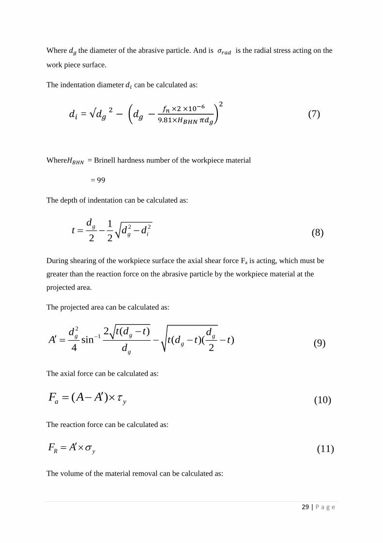
Where the diameter of the abrasive particle. And is is the radial stress acting on the

work piece surface.

The indentation diameter can be calculated as:

= (

)

(7)

Where = Brinell hardness number of the workpiece material

=

The depth of indentation can be calculated as:

2 21

2 2

g

g i

dt d d (8)

During shearing of the workpiece surface the axial shear force Fa is acting, which must be

greater than the reaction force on the abrasive particle by the workpiece material at the

projected area.

The projected area can be calculated as:

2

12 ( )

sin ( )( )4 2

gg g

g

g

t d td dA t d t t

d

(9)

The axial force can be calculated as:

( )a yF A A (10)

The reaction force can be calculated as:

R yF A (11)

The volume of the material removal can be calculated as:

30 | P a g e

(12)

Where is the contact length of grain on the with the work piece.

(13)

Where is the contact angle of abrasive grain on the work piece.

Can be calculated as (14)

31 | P a g e

3.2 Simulation on a cylindrical pipe:

Presently the CFD simulation of flow inside a pipe is also done.

Materials used:

Work piece: Al alloy

Yield strength=

Media: polyborosiloxane + grease

Density= , viscosity=

Abrasive particle: silicon carbide (diameter )

Workpiece design: the work piece is designed by GAMBIT and the meshed.

Figure No. 17: The modelling and meshing of pipe

Diameter of the pipe: no.

Length of pipe :

3.2.1 Simulation through CFD (FLUENT: ANSYS 13):

In this study solid –liquid multi-phase flow mixture model is taken, with solver

double precision and a low Reynolds number [31-36].

Boundary conditions:

Velocity inlet, pressure outlet, symmetrical centreline, Medium density is and

viscosity of Operating entrance pressure of and exit pressure is

atmospheric.

Simulation: taking number iteration Reporting interval = 1

Iterations are stopped when the residuals for the two component velocity and the continuity

equation approached an asymptotic value.

32 | P a g e

Chapter 4

4.1 Result and discussion for Flat work-piece

In this study the simulation results of fluid flow analysis at different volume fraction

and different extrusion pressure are discussed. Then calculation is made to find the various

parameters like axial force, normal force, and volume of material removal by getting the

results from the simulation.

4.1.1 Velocity distribution:

Figure No.18: Velocity distribution

From the figure we can conclude that the velocity changes when it reaches the taper exit,

magnitude of velocity is maximum at the centre and decreases gradually towards the wall,

because the effect of viscosity present in the media.

Figure No. 19: Velocity distribution on full view of work piece

33 | P a g e

4.1.2 Plot of velocity magnitude with position:

Figure No. 20: Velocity magnitude with position

From the plot of velocity we can determine that the velocity increases slowly up to the end of

taper and then increases suddenly and then becomes constant.

4.1.3 Distribution of velocity vector:

Figure No. 21: Distribution of velocity vector

34 | P a g e

4.1.4 Pressure distribution:

Figure No. 22: Pressure distribution

From the pressure distribution in the region of work piece fixture it remains constant upto the

exit of the taper. After that it decreases gradually to the end of the workpiece.

Figure No. 23: Pressure distribution of full view of work piece

35 | P a g e

4.1.5 Plot of static pressure with position:

Figure No. 24: Static pressure with position

From the XY plot pressure distribution we conclude that initially the pressure is maximum at

the inlet. It remains constant up to the taper then it starts decreasing gradually.

4.1.6 Strain distribution:

Figure No. 25: Strain distribution

From the figure above we can conclude that the strain is maximum at the wall. That’s why

stress will be produced there to remove the material.

36 | P a g e

Figure No. 26: Strain distribution of full view of work piece.

4.1.7 Plot of strain rate with position:

Figure No. 27: Strain rate with position

From the XY plot of strain distribution it is observed that, it is initially zero and then

increases up to certain distance and then decreases up to distance 20 mm.Then it increases

suddenly to its maximum value and then decreases and then becomes constant.

37 | P a g e

4.1.8 Plot of axial wall shear stress with position:

Figure No. 28: Axial wall shear stress with position

4.1.9 Plot of radial wall shear stress with position:

Figure No. 29: Radial wall shear stress with position

From CFD calculation the radial stress on the work piece material is,

Putting the value of radial stress on equation no. 5, we get normal force

38 | P a g e

Now the indentation diameter can be calculated by putting the value of in equation no. 7

= 4.328*10-7

Putting the value of in equation no 8. We get

Depth of indentation, =

Then projected area can be calculated as putting the value o in equation no. 9.

=

Now the reaction force can be calculated by putting the values in equation no.11

=

From the CFD calculation the axial stress on the workpiece material is ,

Now axial force can be calculated by putting the value of in equation no. 10

=

From the above calculation of axial force and reaction force we have found that the axial

force is very much higher (104

times) than the reaction force. This signifies that the shearing

action or the material removal from the work piece surface has been taken place.

Also from the equation no.14 we get,

Also we know

So

Now the volume of the material can be calculated from equation no. 12,

=

39 | P a g e

4.2 Results and discussion of flow inside a pipe:

After the iteration is stopped the velocity and pressure distribution, the axial stress and

the radial stresses are found as follows.

4.2.1 Velocity distribution:

Figure No. 30: Velocity distribution

From the simulation of velocity it is found that the velocity is maximum at the centreline and

is minimum at the wall.

4.2.2 Plot of velocity magnitude with position:

Figure No. 31: Velocity magnitude with in radial direction

40 | P a g e

4.2.3 Pressure distribution:

Figure No. 32: Pressure distribution

From the figure of pressure distribution it is found that the pressure decreases gradually from

inlet to outlet.

4.2.4 Plot of Variation of pressure in axial direction:

Figure No. 33: Static pressure with position

41 | P a g e

4.2.5 Plot of axial wall shear stress:

Figure No. 34: Axial wall shear stress with position

4.2.6 Plot of radial wall shear stress:

Figure No. 35: Radial wall shear stress with position

From CFD calculation the radial stress on the work piece material is,

Putting the value of radial stress on equation no. 5 the normal force is found to be,

42 | P a g e

Now the indentation diameter can be calculated by putting the value of in equation no. 7

=

Putting the value of in equation no.8 it is found that

Depth of indentation =

Then projected area can be calculated as putting the value of ‘in equation no.9

=

Now the reaction force can be calculated by putting the values in equation no. 11

N

From the CFD calculation the axial stress on the workpiece material is

Now axial force can be calculated by putting the values in equation no. 10

From the above calculation of axial force and reaction force we have found that the axial

force is very much higher (105

times) than the reaction force.which signifies that the shearing

action or the material removal from the work piece surface has been taken place.

Also from the equation no.14, can be calculated as:

So the contact length is

Now the volume of the material can be calculated by putting the values in equation no.12

43 | P a g e

Chapter 5

Optimization

Machinability of a material indicates towards adaptability to be manufactured by a

machining process. In general, machinability can be defined as an optimal combination of

factors such as low cutting force, high material removal rate, good surface integrity, accurate

and consistent workpiece geometrical characteristics. There are various methods of

optimization available. In this study we have used the Response surface methodology to

optimize the work.

5.1 Response Surface Methodology:

Mainly response surface methodology (RSM) was carried out in this study. Usually,

the correlation between the dependent variables and independent variables is either extremely

complex. However, RSM gives a procedure which solves this problem [37, 39]. Assume that

the decision maker is concerned with a system involving a dependent variable Y, which

affects on the independent variable xj. It is also taken that xj is continuous and convenient.

With RSM, the functional relationship between the output y and the levels of n input

parameters can be written as:

(15)

A mathematical model for such a relationship does not necessarily exist. Thus, the

first step in RSM is to get a suitable approximation for using a low-order

polynomial in some section of the independent variables. If the approximated function has

linear variables, a first-order polynomial can be used and written in terms of the independent

variables:

(16)

Otherwise, a second-order polynomial can be used:

∑ +∑

∑ ∑

(17)

The common use of second-order polynomial models is justified by the fact that they

influence the nonlinear behavior of the system. Experimental designs for setting a second-

order response surface must entail at least three levels of each variable so that the coefficients

44 | P a g e

in the model can be predictable. A rotation characteristic is required for response surface

models because the orientation of the design, with respect to its surface, is unidentified.

Hence, the orientation of the design is an important factor in regard to the response surface

which affects the set of data and the fitting of the response surface. Here the DOE of three

parameters with box-behnken design of 15 run conducted and that can be used for setting a

second-order model to the response surface [37, 39]. This study used the Box–Behnken

design because it allowed for fruitful estimation of the first-order and second-order

coefficients. Using this experimental design, the levels of each parameter were assumed to be

equally spaced. A least-squares method was used to approximate the coefficients to

approximate the polynomials. The response surface analysis then proceeded in terms of the

fitted surface. If the fitted surface is an enough estimation of the true functional relationship,

then the analysis of the fitted response will be nearly correspondent to the analysis of the

studied problem. Based on the RSM results, the design engineer can select the critical process

controllable variables for reducing the variation in quality value significantly. The ultimate

goal of RSM is to decide the optimal factor levels and to form the prediction function in the

system. The MINITAB version 16 software was used to develop the experimental plan for

RSM. The same software was also used to analyze the data collected by following the steps

[39]:

1) Choose a transformation if desired. Otherwise, leave the option at “None”.

2) Select the suitable model to be used. The Fit Summary button shows the sequential F-tests,

lack-of-fit tests and other adequacy measures that could be used to help in selecting the

appropriate model.

3) Perform the analysis of variance (ANOVA) analysis of individual model coefficients and

case information for analysis of residuals.

4) Inspect various diagnostic graphs to statistically validate to the model.

5) If the model looks good, generate model graphs, i.e. the contour and 3D graphs, for

analysis. The study and inspection performed in steps (3) and (4) above will illustrate

whether the model is good or otherwise. Very briefly, best model must be significant and the

lack-of-fit must be insignificant.

45 | P a g e

5.1.1 Optimization techniques

Mathematical programming can represent one problem formulation that normalizes

all deterministic operations research methodologies [39].The problem formulation is

represented as:

Optimize (18)

Subject to (19)

(20)

Where j is 1, 2, 3 ... n, i is 1, 2, 3.... m.

In this study, was the concerned objective function with as

the controllable variable. should fall between the mentioned low limit ,and the upper

limit .The objective functions are less important

than . Thus, these objective functions are considered as constraints for

multiple objective optimizations. For example, Eq. (4) is this type of constraint. The

constraints should fall within the domain of .

5.1.2 Test for significance of the regression model

This test is performed as an ANOVA analysis by calculating the F-ratio, which is the

ratio between the regression mean square and the mean square error. The F-ratio, also called

the variance ratio, is the ratio of variance due to the effect of a variable and variance due to

the error term. This ratio is used to calculate the significance of the model under investigation

with respect to the variance of all the terms incorporated in the error term at the desired

significance α-level. A significant model is preferred.

5.1.3 Test for significance on individual model coefficients

This test structures the basis for model optimization by adding or deleting coefficients

through backward elimination, for-ward addition or stepwise elimination/addition/exchange.

It engages the determination of the P-value or probability value, usually relating the risk of

falsely refusing a given hypothesis. For example, a “Prob. Value > F” value on an F-test

46 | P a g e

informs the proportion of time you would anticipate to get the stated F-value if no factor

effects are significant. The “Prob. Value > F” determined can be compared with the preferred

probability or α-level. In general, the lowest order polynomial would be selected to

adequately describe the system.

5.1.4 Test for lack-of-fit

As imitate measurements are available, a test indicating the consequence of the

replicate error in comparison to the model dependent error can be performed. This test

divides the residual or error sum of squares into two portions, one which is due to pure error

which is based on the replicate measurements and the other due to lack-of-fit based on the

model results. The test statistic for lack-of-fit is the ratio in between the lack-of-fit mean

square and the pure error mean square. As previously, this F-test statistic can be used to find

out as to whether the lack-of-fit error is significant or otherwise at the desired significance α-

level. Insignificant lack-of-fit is desired as significant lack-of-fit designates that there might

be contributions in the regression of response relationship that are not reported for by the

model.

5.2 Results and discussions:

In this present study, the characteristic parameters of abrasive flow machining are

taken of 3 variables and their domains are shown in Table no. 1 with high and low value.

Here the Response Surface Methodology (RSM) is used for optimization of this operation.

RSM is an efficient and fruitful method of optimization in statistical analysis. Design of

Experiment (DOE) of above said three parameters with 15 runs is given in Table no. 2. The

input variables of this machining are volumetric fraction, pressure and velocity which are

tabulated in Table no. 3 with their standard and experimental run order. Then the out

responses i.e. axial stress, radial stress and indentation depth are recorded in Table no. 4. For

this optimization Minitab version 16 is utilized and gives 3D surface plots below.

47 | P a g e

Table No. 1: Value of Input Process Parameters

Process parameters Unit Code Low High

Volume fraction % A 40 50

Pressure Bar B 35 60

Velocity m/sec C 0.009 0.025

Table No. 2: Design Table Randomized

RUN BLOCK A B C

1 1 + 0 -

2 1 0 - -

3 1 - - 0

4 1 0 + +

5 1 0 0 0

6 1 0 0 0

7 1 0 + -

8 1 0 - +

9 1 + + 0

10 1 0 0 0

11 1 + - 0

12 1 - + 0

13 1 + 0 +

14 1 - 0 +

15 1 - 0 -

48 | P a g e

Table No. 3: Design table

Std. Order Run Order VOLUME

FRACTION PRESSURE VELOCITY

6 1 50 47.5 0.009

9 2 45 35.0 0.009

1 3 40 35.0 0.017

12 4 45 60.0 0.025

15 5 45 47.5 0.017

14 6 45 47.5 0.017

10 7 45 60.0 0.009

11 8 45 35.0 0.025

4 9 50 60.0 0.017

13 10 45 47.5 0.017

2 11 50 35.0 0.017

3 12 40 60.0 0.017

8 13 50 47.5 0.025

7 14 40 47.5 0.025

5 15 40 47.5 0.009

49 | P a g e

Table No. 4: Value of Output responses

Run Order AXIAL STRESS RADIAL STRESS INDENTATION

DEPTH

1 41.064 0.236 1.340

2 30.142 0.092 1.080

3 30.052 0.069 1.070

4 46.987 0.286 1.876

5 40.764 0.219 1.241

6 40.981 0.221 1.253

7 45.894 0.275 1.864

8 30.239 0.108 1.092

9 47.234 0.296 1.982

10 40.542 0.241 1.261

11 30.438 0.139 1.116

12 45.564 0.261 1.881

13 40.763 0.209 1.219

14 40.439 0.275 1.283

15 40.018 0.237 1.249

50 | P a g e

Axial stress:

The regression analysis is carried out for the given output responses. First the

regression table axial stress is shown in Table no. 5 in which pressure, the square term of

pressure and the interaction between volume fraction and pressure have significant value as

their values are less than p=0.05. Here R-square value comes 99.94 % which is acceptable.

Then Analysis of Variance (ANOVA) analysis for axial stress has been done in Table no. 6 in

which the total degree of freedom of input parameters is 14.

Table No. 5: Estimated Regression Coefficients for AXIAL STRESS

TERM COEFFICIENT SE

COEFFICIENT

T P

CONSTANT -26.52 11.77 -2.254 0.074

VOLUME FRACTION 0.25 0.47 0.530 0.619

PRESSURE 1.80 0.12 15.017 0.000

VELOCITY 157.81 165.33 0.954 0.384

VOL.FRACTION*VOL.FRACTION -0.00 0.01 0.721 0.503

PRESSURE*PRESSURE -0.02 0.00 -18.330 0.000

VELOCITY*VELOCITY -1545.57 2001.44 -0.772 0.475

VOL.FRACTION*PRESSURE 0.01 0.00 2.608 0.408

VOL.FRACTION*VELOCITY -4.51 3.08 -1.467 0.202

PRESSURE*VELOCITY 2.49 1.23 2.023 0.099

S = 0.246134 PRESS = 3.52154

R-Sq. = 99.94%, R-Sq. (pred) = 99.36%, R-Sq. (adj) = 99.85%

51 | P a g e

Table No. 6: Analysis of Variance for AXIAL STRESS:

SOURCE DF SEQ SS Adj SS Adj MS F

REGRESSION 9 547.887 547.887 60.8763 1004.86

LINEAR 3 526.691 14.020 4.6734 77.14

VOL.FRACTION 1 1.467 0.017 0.0170 0.28

PRESSURE 1 525.010 13.661 13.6610 225.50

VELOCITY 1 0.215 0.055 0.0552 0.91

SQUARE 3 20.405 20.405 6.8016 112.27

VOL.FRACTION*VOLFRACTION 1 0.025 0.032 0.0315 0.52

PRESSURE*PRRESSURE 1 20.343 20.335 20.3546 335.99

VELOCITY*VELOCITY 1 0.036 0.036 0.0361 0.60

INTERACTION 3 0.790 0.790 0.2635 4.35

VOL.FRACTION*PRESSURE 1 0.412 0.412 0.4122 6.80

VOL.FRACTION*VELOCITY 1 0.130 0.130 0.1303 2.15

PRESSURE*VELOCITY 1 0.248 0.248 0.2480 4.09

RESIDUAL ERROR 5 0.303 0.303 0.0606 -

LACK OF FIT 3 0.207 0.207 0.0688 1.43

PURE ERROR 2 0.096 0.096 0.0482 -

TOTAL 14

The first order quadratic equation is generated which is given below:

AXIAL STRESS = 4.42000 + 0.08570* A + 0.64800*B + 20.50000*C (21)

52 | P a g e

Radial stress:

The regression analysis for radial stress is shown in table no 8.In which the pressure,

the square term of pressure have significant value as their values are less than 0.05. Here R-sq

value comes 94.46% which is acceptable. The analysis of variance for radial stress has been

done in table no.9 in which total degree of freedom of input parameters are 14.

Table No.7: Estimated Regression Coefficients for RADIAL STRESS

TERM COEF. SE COEF. T P

CONSTANT -0.8331 1.360 -0.613 0.567

VOL.FRACTION -0.0093 0.055 -0.171 0.871

PRESSURE 0.0394 0.014 2.840 0.036

VELOCITY 16.4805 19.013 0.863 0.428

VOL.FRACTION*VOL.FRACTION 0.0003 0.001 0.448 0.673

PRRESSURRE*PRESSURE -0.003 0.000 -2.863 0.035

VELOCITY*VELOCITY 87.8906 231.255 0.380 0.720

VOL.FRACTION*PRESSURE -0.0001 0.000 -0.615 0.565


PRESSURE*VELOCITY -0.0125 0.0142 -0.088 0.933

S = 0.0284394 PRESS = 0.060634

R-Sq = 94.68%, R-Sq (pred) = 20.25% R-Sq (adj) = 85.11%

53 | P a g e

Table No. 8: Analysis of Variance for RADIAL STRESS

SOURCE DF Seq SS Adj SS AdJ MS F

REGRESSION 9 0.071985 0.071985 0.007998 9.89

LINER 3 0.063373 0.007376 0.002459 3.04

VOL.FRACTION 1 0.000180 0.000024 0.000024 0.03

PRESSURE 1 0.063012 0.006522 0.006522 8.06

VELOCITY 1 0.000180 0.000602 0.000602 0.74

SQUARE 3 0.007243 0.007243 0.002414 2.98

VOL.FRACTION*VOL.FRACTION 1 0.000319 0.000162 0.000162 0.20

VOL.FRACTION*PRESSURE 1 0.006806 0.006630 0.006630 8,20


INTERACTION 3 0.001369 0.001369 0.000456 0.56


VOL.FRACTION*VELOCITY 1 0.001056 0.001056 0.001056 1.31


RESIDUAL ERROR 5 0.004044 0.004044 0.000809 -

LACK OF FIT 3 0.003748 0.003748 0.001249 8.44

PURE ERROR 2 0.000296 0.000296 0.111148 -

TOTAL 14

The first order quadratic equation is generated which is given below.

RADIAL STRESS = - 0.17900 + 0.00095*A + 0.00710*B + 0.59000*C (22)

54 | P a g e

Depth of indentation:

The regression analysis of depth of indentation is shown in table no.9.in which the

pressure and the square term of pressure have significant value as their values are less than

0.05.Here R-sq value comes as 99.67% which is acceptable. The analysis of variance for

depth of indentation has been done in table no .10, in which total no. of degree of freedom of

input parameters are 14.

Table No. 9: Estimated Regression Coefficients for INDENTATION DEPTH

TERM COEFF. SE COEFF T P

CONSTANT 4.835 1.516 3.189 0.024

VOL.FRACTION -0.089 0.061 -1.462 0.204

PRESSURE -0.119 0.015 -7.700 0.001

VELOCITY 46.107 21.301 2.165 0.083

VOL.FRACTION*VOLFRACTION 0.001 0.001 1.676 0.154

PRESSURRE*PRESSURE 0.001 0.000 14.144 0.000

VELOCITY*VELOCITY -102.865 157.858 -0.399 0.706

VOL.FRACTION*PRRESSURE 0.000 0.000 8.867 0.425


PRESSURE*VELOCITY 0.000 0.159 0.000 1.000

S = 0.0317109 PRESS = 0.07766

R-Sq = 99.67%, R-Sq (pred) = 94.94%, R-Sq (adj) = 99.08%

55 | P a g e

Table No. 10: Analysis of Variance for INDENTATION DEPTH

SOURCE DF Seq SS Adj SS Adj MS F

REGRESSION 9 1.53033 1.53033 0.170036 169.09

LINER 3 1.32053 0.0673 0.022542 22.42

VOL.FRACTION 1 0.00378 0.00215 0.002149 2.14

PRESSURE 1 1.31625 0.05963 0.59628 59.30

VELOCITY 1 0.00050 0.00471 0.004711 4.69

SQUARE 3 0.20303 0.20303 0.067677 67.30

VOL.FRACTION*VOL.FRACTION 1 0.00049 0.00283 0.002826 2.81

PRESSURE*PRESSURE 1 0.20238 0.20031 0.200308 199.20

VELOCITY*VELOCITY 1 0.00016 0.00016 0.000160 0.16

INTERACTION 3 0.00676 0.00676 0.002254 2,24


VOL.FRACTUION*VELOCITY 1 0.00601 0.00601 0.006006 5.97


RESIDUAL ERROR 5 0.00503 0.00503 0.001006 -

LACK OF FIT 3 0.00483 0.00483 0.001608 15.87

PURE ERROR 2 0.00020 0.00101 0.000101 -

TOTAL 14

The first order quadratic equation is generated which is given below.

INDENTATION DEPTH = - 0.33300 + 0.00435*A+ 0.03250*B - 0.98000*C (23)

56 | P a g e

5.2.1 Residual plots:

Axial stress:

3210-1-2-3

99

95

90

80

70

60

50

40

30

20

10

5

1

Standardized Residual

Pe

rce

nt

Normal Probability Plot(response is AXIAL STRESS)

48464442403836343230

2

1

0

-1

-2

Fitted Value

Sta

nd

ard

ize

d R

esid

ua

l

Versus Fits(response is AXIAL STRESS)

Figure. No. 36 Figure. No. 37

210-1-2

3.0

2.5

2.0

1.5

1.0

0.5

0.0


Fre

qu

en

cy

Histogram(response is AXIAL STRESS)

151413121110987654321

2

1

0

-1

-2

Observation Order

Sta

nd

ard

ize

d R

esid

ua

l

Versus Order(response is AXIAL STRESS)

Figure No. 38 Figure No.39

The normal probability plot of output response of axial stress is plotted in Fig. no. 36

in which almost all the points are situated on the straight line. Thus, the results which are

obtained for axial stress are correct. Then fitted value vs. standardized residual value plot is

given in Fig. no. 37. In this graph no pattern of these points is formed. So, the input

parameters are fitted well in 95 % confidence interval. The histogram plot of axial stress is

shown in Fig. no. 38 in which all the columns are formed into normal probability distribution.

Therefore, the present result indicates the realistic analysis of abrasive flow machining which

is carried out in a successful manner. The plot between standardized order and residual values

is presented in Fig. no. 39 where minimum axial stress is occurred in the 13th

run and

similarly at the 15th

run the maximum value is obtained.

57 | P a g e

Radial stress:

3210-1-2-3

99

95

90

80

70

60

50

40

30

20

10

5

1


Pe

rce

nt

Normal Probability Plot(response is RADIAL STRESS)

0.300.250.200.150.10

2

1

0

-1

-2

Fitted Value

Sta

nd

ard

ize

d R

esid

ua

l

Versus Fits(response is RADIAL STRESS)

Figure No.40: Figure No. 41:

1.51.00.50.0-0.5-1.0-1.5

4

3

2

1

0


Fre

qu

en

cy

Histogram(response is RADIAL STRESS)

151413121110987654321

2

1

0

-1

-2

Observation Order

Sta

nd

ard

ize

d R

esid

ua

l

Versus Order(response is RADIAL STRESS)

Figure No. 42: Figure No. 43:

The normal probability plot of output response of radial stress is plotted in Fig. no. 40

in which almost all the points are situated on the straight line. Thus, the results which are

obtained for radial stress are correct. Then fitted value vs. standardized residual value plot is

given in Fig. no. 41. In this graph no pattern of these points is formed. So, the input

parameters are fitted well in 95 % confidence interval. The histogram plot of radial stress is

shown in Fig. no. 42 in which all the columns are formed into normal probability distribution.

Therefore, the present result indicates the realistic analysis of abrasive flow machining which

is carried out in a successful manner. The plot between standardized order and residual values

is presented in Fig. no. 43 where minimum radial stress is occurred in the 13th

run and

similarly at the 11th


58 | P a g e

Indentation depth:

3210-1-2-3

99

95

90

80

70

60

50

40

30

20

10

5

1


Pe

rce

nt

Normal Probability Plot(response is INDENTATION DEPTH)

2.01.81.61.41.21.0

2

1

0

-1

-2

Fitted ValueS

ta

nd

ard

ize

d R

esid

ua

l

Versus Fits(response is INDENTATION DEPTH)

Figure No. 44: Figure No. 45:

210-1-2

7

6

5

4

3

2

1

0


Fre

qu

en

cy

Histogram(response is INDENTATION DEPTH)

151413121110987654321

2

1

0

-1

-2

Observation Order

Sta

nd

ard

ize

d R

esid

ua

l

Versus Order(response is INDENTATION DEPTH)

Figure No. 46 Figure No. 47

The normal probability plot of output response of indentation depth is plotted in Fig.

no. 44 in which almost all the points are situated on the straight line. Thus, the results which

are obtained for indentation depth are correct. Then fitted value vs. standardized residual

value plot is given in Fig. no. 45. In this graph no pattern of these points is formed. So, the

input parameters are fitted well in 95 % confidence interval. The histogram plot of

indentation depth is shown in Fig. no. 46 in which all the columns are formed into normal

probability distribution. Therefore, the present result indicates the realistic analysis of

abrasive flow machining which is carried out in a successful manner. The plot between

standardized order and residual values is presented in Fig. no. 47 where minimum indentation

depth is occurred in the 13th

run and similarly at the 9th


59 | P a g e

5.2.2 Contour plots:

Axial stress:

50

30 45

35

40

45

4050 40

60

AXIAL STRESS

VOLUME FRACTION

PRESSURE

PLOT NO. 1 Contour Plot of AXIAL STRESS vs VOLUME FRACTION, PRESSURE

PRESSURE

VO

LU

ME F

RA

CTIO

N

605550454035

50

48

46

44

42

40

>

–

–

–

–

< 33

33 36

36 39

39 42

42 45

45

STRESS

AXIAL

PLOT NO. 1 Contour Plot of AXIAL STRESS vs VOLUME FRACTION, PRESSURE


The 3D contour plot of axial stress vs. interaction of volume fraction and pressure is

presented in Fig. no. 48 which show the plot increases with both increasing in pressure and

volume fraction respectively. The 2D contour plot of axial stress vs. interaction of volume

fraction and pressure is shown in Fig. no. 49.

50

30 45

35

40

45

0.0100.015 40

0.0200.025

AXIAL STRESS

VOLUME FRACTION

VELOCITY

PLOT 2 Surface Plot of AXIAL STRESS vs VOLUME FRACTION, VELOCITY

VELOCITY

VO

LU

ME F

RA

CTIO

N

0.0240.0220.0200.0180.0160.0140.0120.010

50

48

46

44

42

40

>

–

–

–

–

< 33

33 36

36 39

39 42

42 45

45

STRESS

AXIAL

PLOT 2 Surface Plot of AXIAL STRESS vs VOLUME FRACTION, VELOCITY


The 3D contour plot of axial stress vs. interaction of volume fraction and velocity is

presented in Fig. no. 50 which show the plot increases at the middle region of velocity and

volume fraction. The 2D contour plot of axial stress vs. interaction of volume fraction and

velocity is shown in Fig. no. 51.

60 | P a g e

60

5030

35

40

45

0.010 400.015

0.0200.025

AXIAL STRESS

PRESSURE

VELOCITY

PLOT 3 Surface Plot of AXIAL STRESS vs PRESSURE, VELOCITY

VELOCITY

PR

ES

SU

RE

0.0240.0220.0200.0180.0160.0140.0120.010

60

55

50

45

40

35

>

–

–

–

–

< 33

33 36

36 39

39 42

42 45

45

STRESS

AXIAL

PLOT 3 Surface Plot of AXIAL STRESS vs PRESSURE, VELOCITY


The 3D contour plot of axial stress vs. interaction of velocity and pressure is presented in Fig.

no. 52 which show the plot increases with increasing by pressure and remains constant with

velocity. The 2D contour plot of axial stress vs. interaction of velocity and pressure is shown

in Fig. no. 53.

Radial stress:

50

0.1

45

0.2

0.3

4050 40

60

RADIAL STRESS

VOLUME FRACTION

PRESSURE

PLOT 4 Surface Plot of RADIAL STRESS vs VOLUME FRACTION, PRESSURE

PRESSURE

VO

LU

ME F

RA

CTIO

N

605550454035

50

48

46

44

42

40

>

–

–

–

< 0.10

0.10 0.15

0.15 0.20

0.20 0.25

0.25

STRESS

RADIAL

PLOT 4 Surface Plot of RADIAL STRESS vs VOLUME FRACTION, PRESSURE


The 3D contour plot of radial stress vs. interaction of volume fraction and pressure is

presented in Fig. no. 54 which show the plot increases with increasing in pressure in high

manner and in case of volume fraction it increases slowly. The 2D contour plot of radial

stress vs. interaction of volume fraction and pressure is shown in Fig. no. 55.

61 | P a g e

50

0.1

45

0.2

0.3

0.0100.015 40

0.0200.025

RADIAL STRESS

VOLUME FRACTION

VELOCITY

PLOT 5 Surface Plot of RADIAL STRESS vs VOLUME FRACTION, VELOCITY

VELOCITY

VO

LU

ME F

RA

CTIO

N

0.0240.0220.0200.0180.0160.0140.0120.010

50

48

46

44

42

40

>

–

–

–

< 0.10

0.10 0.15

0.15 0.20

0.20 0.25

0.25

STRESS

RADIAL

PLOT 5 Surface Plot of RADIAL STRESS vs VOLUME FRACTION, VELOCITY


The 3D contour plot of radial stress vs. interaction of volume fraction and velocity is

presented in Fig. no. 56 which show the plot increases at the middle region of velocity and

volume fraction. The 2D contour plot of radial stress vs. interaction of volume fraction and

velocity is shown in Fig. no. 57.

60

50

0.1

0.2

0.3

0.010 400.015

0.0200.025

RADIAL STRESS

PRESSURE

VELOCITY

PLOT 6 Surface Plot of RADIAL STRESS vs PRESSURE, VELOCITY

VELOCITY

PR

ES

SU

RE

0.0240.0220.0200.0180.0160.0140.0120.010

60

55

50

45

40

35

>

–

–

–

< 0.10

0.10 0.15

0.15 0.20

0.20 0.25

0.25

STRESS

RADIAL

PLOT 6 Surface Plot of RADIAL STRESS vs PRESSURE, VELOCITY


The 3D contour plot of radial stress vs. interaction of velocity and pressure is presented in

Fig. no. 58 which show the plot increases with increasing by pressure and remains almost

constant with velocity. The 2D contour plot of radial stress vs. interaction of velocity and

pressure is shown in Fig. no. 59.

62 | P a g e

Indentation depth:

50

1.0 45

1.5

2.0

4050 40

60

INDENTATION DEPTH

VOLUME FRACTION

PRESSURE

PLOT 7 Surface Plot of INDENTATION DEPTH vs VOLUME FRACTION, PRESSURE

PRESSURE

VO

LU

ME F

RA

CTIO

N

605550454035

50

48

46

44

42

40

>

–

–

–

–

–

< 1.20

1.20 1.35

1.35 1.50

1.50 1.65

1.65 1.80

1.80 1.95

1.95

DEPTH

INDENTATION

PLOT 7 Surface Plot of INDENTATION DEPTH vs VOLUME FRACTION, PRESSURE


The 3D contour plot of indentation depth vs. interaction of volume fraction and

pressure is presented in Fig. no. 25 which show the plot increases with increasing in pressure

and remains constant with volume fraction. The 2D contour plot of indentation depth vs.

interaction of volume fraction and pressure is shown in Fig. no. 26.

50

1.0 45

1.5

2.0

0.0100.015 40

0.0200.025

INDENTATION DEPTH

VOLUME FRACTION

VELOCITY

PLOT 8 Surface Plot of INDENTATION DEPTH vs VOLUME FRACTION, VELOCITY

VELOCITY

VO

LU

ME F

RA

CTIO

N

0.0240.0220.0200.0180.0160.0140.0120.010

50

48

46

44

42

40

>

–

–

–

–

–

< 1.20

1.20 1.35

1.35 1.50

1.50 1.65

1.65 1.80

1.80 1.95

1.95

DEPTH

INDENTATION

PLOT 8 Surface Plot of INDENTATION DEPTH vs VOLUME FRACTION, VELOCITY


The 3D contour plot of indentation depth vs. interaction of volume fraction and velocity is

presented in Fig. no. 62 which show the plot decreases with respect to the middle region of

velocity and volume fraction. The 2D contour plot of indentation depth vs. interaction of

volume fraction and velocity is shown in Fig. no. 63.

63 | P a g e

60

501.0

1.5

2.0

0.010 400.015

0.0200.025

INDENTATION DEPTH

PRESSURE

VELOCITY

PLOT 9 Surface Plot of INDENTATION DEPTH vs PRESSURE, VELOCITY

VELOCITY

PR

ES

SU

RE

0.0240.0220.0200.0180.0160.0140.0120.010

60

55

50

45

40

35

>

–

–

–

–

–

< 1.20

1.20 1.35

1.35 1.50

1.50 1.65

1.65 1.80

1.80 1.95

1.95

DEPTH

INDENTATION

PLOT 9 Surface Plot of INDENTATION DEPTH vs PRESSURE, VELOCITY


The 3D contour plot of indentation depth vs. interaction of velocity and pressure is presented

in Fig. no. 64 which show the plot increases with increasing by pressure and remains constant

with velocity. The 2D contour plot of indentation depth vs. interaction of velocity and

pressure is shown in Fig. no. 65.

64 | P a g e

Chapter 6

Conclusion

The present study develops CFD simulation of AFM in a flat workpiece and in a pipe

taking different input parameters and then the results are verified. The present study also

develops optimization for AFM process of Al. alloy using response surface method. It is

found that all the three machining parameters and some of their interactions have significant

effect on outputs considered in the present study. Finally, an attempt has been made to

estimate the optimum machining conditions to produce the best possible output within the

experimental constraints.

From CFD analysis it is found the axial stress, radial stress at the workpiece surface

and then the axial force and normal forces area calculated.

Material removal rate also calculated from this simulation.

The optimal condition of input variables are at 50 % of volume fraction, 60 bar of

pressure and 0.017 m/s of velocity in this study and also get maximum value of each

output responses.

The ANOVA revealed that the pressure is the most significant factor influencing the

response variables examined.

Additionally, the volume fraction and velocity also provided secondary contribution

to the out responses.

The reduced linear models developed using RSM were reasonably perfect and can be

used for prediction within the limits of the factors investigated.

65 | P a g e

Chapter 7

Refrences

[1] Gorana, V.K., Jain, V.K., Lal, G.K., 2004, Experimental investigation into cutting forces

and active grain density during abrasive flow machining, International Journal of Machine

Tool & Manufacture, Vol. 44, pp. 201-211.

[2] Gorana V. K, Jain V. K. and Lal G. K. “Prediction of surface roughness during abrasive

flow machining”, The International Journal of Advanced Manufacturing Technology,

2006,(31):258-267

[3] Jain R.K, Jain V.K, Simulation of surface generated in abrasive flow machining, Robotics

and Computer Integrated Manufacturing 15 (1999) 403–412.

[4] Lal G.K., Forces in vertical surface grinding, International Journal of Machine Tool

Design Research 8 (1968) 33–43.

[5] Jain R.K, Jain V.K, Dixit P.M. Modelling of material removal and surface rough-ness in

abrasive flow machining process, International Journal of Machine Tools & Manufacture 39

(1999) 1903–1923

[6] Jha. S, Jain V.K, Design and development of the magneto rheological abrasive flow

finishing process, International Journal of Machine Tools & Manufacture 44 (2004) 1019-

1029.

[7] Jha S, Jain V.K, Modelling and simulation of surface roughness in magneto rheological

abrasive flow finishing (MRAFF) process, Wear 261 (2006) 856–866.

[8] Das M, Jain V. K and Ghoshdastidar P.S Computational fluid dynamics simulation and

experimental investigations into the magnetic-field-assisted nano-finishing process (2012).

[9] Jayswal S.C, Jain V.K, Dixit P.M. Modelling and simulation of magnetic abrasive

finishing process, International Journal of Advanced Manufacturing Technology 26 (2005)

477–490.

[10] Singh, S., Shan, H.S., Kumar, P., 2002, Wear behaviour of materials in magnetically

assisted abrasive flow machining, Journal of Materials Processing Technology, Vol. 128, pp.

155- 161.

[11] Rhoades L.J, Abrasive flow machining, Manufacturing Engineering (1988) 66-82.

[12] Rhoades L.J, Abrasive flow machining with not-so-silly putty, Metal Finishing July

(1987) 22-28.

66 | P a g e

[13] Rhoades L.J, Abrasive flow machining: a case study, Journal of Material Processing

Technology 28 (1991) 101-117.

[14] Rhoades, L.J., 1989, Abrasive Flow Machining, Technical Paper of the Society of

Manufacturing Engineers (SME), MR89 – 145.

[15] Przylenk K, AFM—a process for surface finishing and deburring of the workpiece with

a complicated shape by means of an abrasive laden medium, PED, 22ASME, NewYork,1986,

pp. 98-116.

[16] Williams R.E, Rajurkar K.P, Metal removal and surface finish characteristics in abrasive

flow machining, PED, 38ASME, New York, 1989, pp. 87–104.

[17] Loveless T.R, Willams R.E, Rajurkar K.P, A study of the effects of abrasive flow

finishing on various machined surfaces, Journal of Material Processing Technology 47 (1994)

127-142.

[18] Williams R.E. Rajurkar K.P, Stochastic modeling and analysis of abrasive flow

machining, Transactions of the ASME, Journal of Engineering for Industry 114 (1992) 7481.

[19] Williams R.E, Acoustic emission characteristics of abrasive flow machining,

Transactions of the ASME120 (1998) 264–271.

[20] Williams, R.E., Rajurkar, K.P., Rhoades, L. J., 1989, Performance Characteristics of

Abrasive Flow Machining, Technical Paper of the Society of Manufacturing Engineers

(SME), MR89-806.

[21] William R.E, Rajurkar K.P. Monitoring of abrasive flow machining process using

acoustic emission, S.M. Wu Symposium, vol. I, 1994, pp. 35–41.

[22] Fletcher A.J, Hull J.B, Mackie J, Trengove S.A, Computer modeling of abrasive flow

machining process, Proceedings of the 210 V.K. Gorana et al. / International Journal of

Machine Tools & Manufacture 44 (2004) 201–211 International Conference on Surface

Engineering, Toronto, 1994, pp. 31-47, 1990, pp. 584-611.

[23] Kukreja T.R and Mohan Rakesh “A case study of EPDM rubber media utilized in the

abrasive flow machining process’Rubber India 55 (2003). pp.9 -11

[24] Macosko C.W. Rheology Principles, Measurement & Applications, VCH Publishers

Inc., New York, 1994.

[25] Beverly C.R, Tanner R.I. Numerical analysis of three-dimensional Bingham plastic

flow, Journal of Non-Newtonian Fluid Mechanics 42 (1992) 85–115.

[26] Bird R.B, Stewart W.E, Lightfoot E.N, Transport Phenomena, Wiley, New York, 1960.

[27] Fang,L, Zha, J., Sun, K, Zheng, D, Ma, D., 2009, Temperature as sensitive monitor for

efficiency of work in abrasive flow machining, Wear, Vol. 266, pp. 678-687.

67 | P a g e

[28] Uhlmann,E, Szulczynski, H., 2005, Precise finishing of inner contours with abrasive

flow machining, International Journal for Manufacturing Science & Technology, Vol. 7 (2),

pp. 33-39.

[29] Uhlmann, E, Mhotovic, V, Coenen, A., 2009, Modelling the abrasive flow machining

process on advanced ceramic materials, Journal of Materials Processing Technology, Vol.

209, pp. 6062- 6066.

[30] Sankar, M.R., Jain, V.K, Ramkumar, J., 2007, Abrasive flow machining (AFM): An

Overview, psgias/smart_machine_tools/V.K.Jain.pdf, 22.11.2011.

Fig. 10: FAX for different end piece geometries at 45 bar piston

[31] Junye Li, Liu Weina, Yang Lifeng, Li Chun, Liu Bin, Wu Haihong and Sun Xiaoli

Design and Simulation for Mico-hole Abrasive Flow Machining (2009) 815-819.

[32] Tzeng Hsinn-Jyh, Yan Biing-Hwa, Hsu Rong-Tzong, and Lin Yan- Cherng. “Self-

modulating abrasive medium and its application to abrasive flow machining for finishing

micro channel surfaces”, TheInternational Journal of Advanced Manufacturing Technology,

2007,(5):1163-1169

[33] Tsai M. J, Huang J. F. “Efficient automatic polishing process with a new compliant

abrasive tool”, The International Journal of Advanced Manufacturing Technology,

2006,(30),817-827

[34] Jain N. K, Jain V. K, and Jha S. “Parametric optimization of advanced fine-finishing

processes”, The International Journal of Advanced Manufacturing Technology, 2007,(34):

1191-1213

[35] Perry, W.B., 1975, Properties and Capabilities of low-pressure abrasive flow media,

Technical Paper of the society of Manufacturing Engineers (SME), MR75-831.

[36] Borchers, J., 1980, Why? Abrasive Flow Deburring, Technical Paper of the Society of

Manufacturing Engineers (SME), MR80 – 101.

[37] R.H. Myers, D.C. Montgomery, Response Surface Methodology-Process and Product

Optimization Using Robust Design, Wiley Series in Probability and Statistics, Wiley, New

York, 1995. pp. 318–321.

[38]D.J. Whitehouse, Handbook of Surface Metrology, Institute of Physics Publishing,

Bristol, UK, 1994

[39] Design-Expert Software, Version 6, User’s Guide, Technical Manual, Stat-Ease Inc.,

Minneapolis, MN, 2000

shakti ranjan garanayak - ethesisethesis.nitrkl.ac.in/4733/1/211me2348.pdf · a thesis submitted in...

Documents