1

Shallow and Deep Lunge Feeding of Humpback Whales in Fjords

of the West Antarctic Peninsula Colin Ware,

Center for Coastal and Ocean Mapping, University of New Hampshire, cware@ccom.unh.edu

Ari S. Friedlaender, Douglas P. Nowacek*,

Nicholas School of the Environment and *Pratt School of Engineering, Duke University Marine

Laboratory, asf7@duke.edu, dpn3@duke.edu.

ABSTRACT

Humpback whales (Megaptera novaeangliae) belong to the class of marine mammals

known as rorquals that feed through extraordinarily energetic lunges during which they engulf

large volumes of water equal to as much as 70% of their body mass. To understand the

kinematics of humpback lunge feeding, we attached high-resolution digital recording tags

incorporating accelerometers, magnetometers, pressure and sound recording to whales feeding on

euphausiids in fjords of the West Antarctic Peninsula. Instances of near vertical lunges gave us

the unique opportunity to use the signal from the accelerometer to obtain a fine scale record of the

body accelerations involved in lunging. We found that lunges contain extreme accelerations

reaching 2.5 m·s-2 in certain instances, which are then followed by decelerations. When animals

are intensively feeding the inter-lunge interval is similar for both deep and shallow lunges

suggesting a biomechanical constraint on lunges. However, the number of lunges per dive varies

from one for shallow feeding (<25m) to a median of six for deeper dives. Different feeding

patterns were evident in the kinematic record, for deep and shallow feeding bouts with the much

greater mean turn rates occurring in shallow feeding.

Keywords: kinematics, lunge feeding, humpback whales

INTRODUCTION

Humpback whales (Megaptera novaeangliae) belong to a group of baleen whales known

as the rorquals that feed by lunging, a technique involving an energetic maneuver to engulf a

volume of water that may equal two thirds of the animal’s body mass (Pivorunas 1979; Brodie

1993; Goldbogen et al. 2007). The water contained in an expanded gular pouch is then pushed out

with the tongue and expelled through baleen plates that act as filters to retain prey. The mouths of

rorqual whales contain a set of extreme morphological and biomechanical adaptations that

facilitate lunge feeding. The enormously enlarged mouth (buccal cavity) extends up to two thirds

of the body length (Matthews 1937). The blubber ventral to the buccal cavity is externally

marked by a series of grooves that extend in a rostral-caudal direction. The ventral groove

blubber is several times more elastic radially than in the rostral-caudal direction and is capable of

being stretched reversibly to several times its resting extent (Brodie 1977, Orton and Brodie

1987). As the mouth opens, the mandibles expand laterally as well as rotating to form roughly a

right angle with the body (Lambersten et al., 1995). Orton and Brodie (1987) estimated that a

speed of 3.0 m·s–1 would generate enough hydrodynamic force to completely inflate the buccal

cavity for fin whales. Enormous hydrodynamic drag results from the lowered mandibles, slowing

the animal and absorbing the kinetic energy gained from the preceding fluke strokes.

Once a prey-filled volume of water has been engulfed, a number of morphological

adaptations combine to augment rapid expulsion and filtering through the baleen. Lambersten et

2

al. (1995) argue that a fibrous frontomandibular stay provides a biological spring between the

frontal bone and the mandibular coronoid, acting in concert with the temporalis muscle to provide

elastic recoil to reverse jaw opening. The lateral expansion of the mandibles also provides a

channel for the lateral expulsion of baleen-filtered seawater once the jaws have closed. The

energy stored in the elastically extended grooved tissues forces water out, assisted by the tongue

and a layer of muscles underlying the blubber (Orton and Brodie 1987). Based on an analysis of

video imagery, Kot (2005) suggested that a rebounding wave within the ventral pouch also

enhances the expulsion of fluid, although more recent modeling work has argued that this is a

reflux (Potvin et al. 2009). Finally, the baleen plates attached to the upper jaw are aligned so as to

provide lateral channels for the expulsion of water, preventing forward jets which would further

slow the animal.

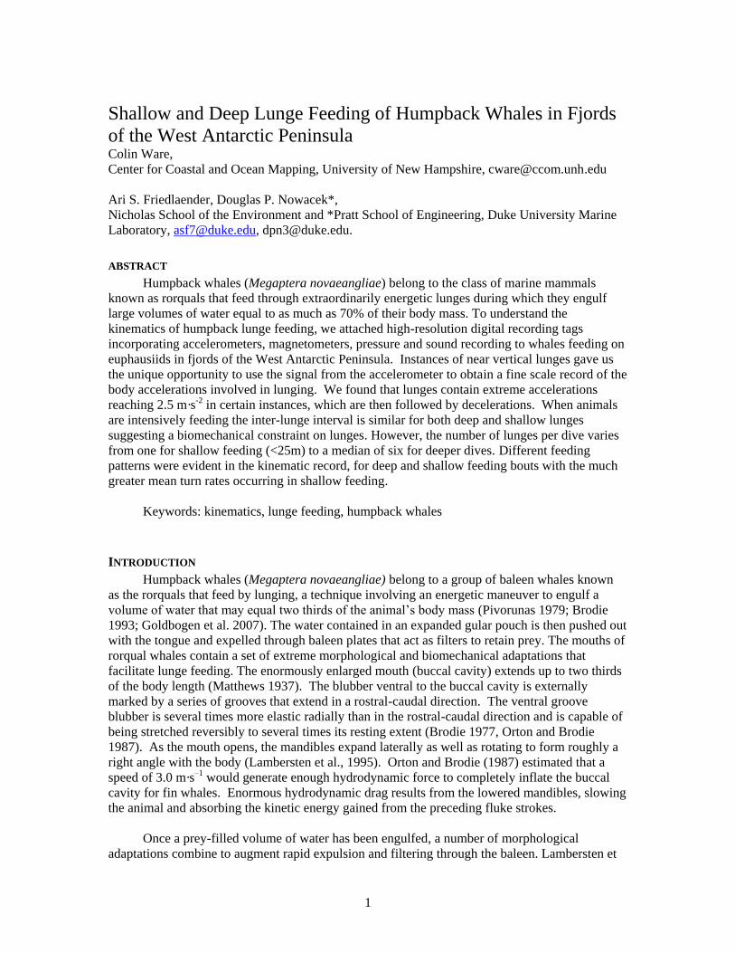
Figure. 1. (A) The acceleration signal measured by tag accelerometers a is the vector sum of gravity g

and the acceleration of the whale’s body w. If the whale acceleration is mostly horizontal (left diagram)

the accelerometers will register little or no change in acceleration. If the whale acceleration is mostly

vertical (right diagram) the accelerometer will register the whale’s acceleration as a deviation from g.

(B) Geometry used to derive a correction factor for speed and pitch angle. The ellipse represents

the attitude of the whale. See text for explanation

a : accelerometer vector

w: whale acceleration

g: gravity

: the measured angle of the whale with respect to the gravity vector.

: the angle correction

Kinematics is the study of motion patterns without regard to the generating forces. Our

current knowledge of lunge feeding kinematics in baleen whales comes mainly from two sources:

visual observations of animals feeding near the surface and data from tagged animals.

Humpback whales feeding near the surface have been observed to exhibit a variety of lunge types

(Jurasz and Jurasz 1979, Sharpe 2001, Hain et al. 1982), including some associated with creating

a net or corral of bubbles (Friedlaender et al. 2009, Hazen et al. 2009). In lateral lunge feeding,

the animal rolls through approximately 90 degrees while feeding. In vertical lunge feeding, the

animal lunges upward, sometimes emerging at the surface with mandibles open and body inverted

(Jurasz and Jurasz, 1979). Similar lateral rolls have been observed in both fin and blue whales

(Watkins and Shevill 1979).

The only source of information regarding baleen whale lunge feeding at depth comes from

digital recording tags attached with suctions cups, containing time and depth recorders, and in the

case of more sophisticated tags, accelerometers and magnetometers to reveal the orientation of

the animal, and sound recording. Goldbogen et al. (2006, 2008) used a tag with two-axis

accelerometers and magnetometers together with acoustic recording to investigate the kinematics

of lunges in fin whales and model underwater lunging behavior in humpback whales.

3

Accelerometer signals, however, were only used to estimate the orientation of the animal, not its

acceleration. The reason for this is that accelerometers can only provide accurate information

about vertical acceleration (see Fig. 1 for an explanation). In order to estimate speed and derive

accelerations they calibrated the recorded flow noise from water rushing past the tag. They

showed that typical fin whale lunges involved three fluke upstrokes and two downstrokes to build

speed with the feeding lunge occurring when the animals were angled upwards at about 30

degrees. Calambokidis et al. (2007) used video imagery and flow noise from a CritterCam®

(National Geographic Society) to infer lunging activity in blue whales. These studies suggest that

fin whales, blue whales and humpbacks have similar lunging strategies.

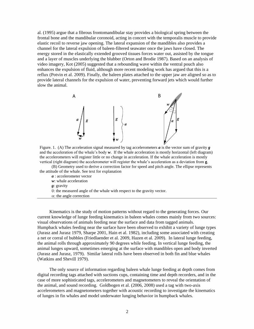
Figure. 2. A representation of a deep foraging dive in TrackPlot. The red and

blue saw tooth patterns on the track are derived from angular accelerations

around a lateral axis and indicators of fluking behavior.

Humpbacks feeding on krill at depth (~100 meters) have been shown to make multiple

lunges per dive, up to a total of 16 in one case (Goldbogen 2008) as measured by the flow noise

method. In an earlier study, Dolphin (1987) had estimated only a single lunge per dive and a dive

rate of approximately 17 dives per hour. It is tacitly assumed that Humpback whales bubble net

feeding near the surface make a single lunge per dive (Jurasz and Jurasz 1979, Friedlaender et al.

2009, Hazen et al. 2009). However, the relationship between the number of lunges per dive and

dive depths has not been reported. In the present study we were able to observe animals carrying

out both shallow and deep foraging dives targeting euphausiid prey over 24 hour periods.

Given the energy and time cost of deep dives, animals should prefer to feed at shallower

depths given equivalent prey abundance (Charnov 1976), although the duration of typical dives is

not long for such a large animal and it has been argued that the major energy expenditure

occurring during deep feeding is due to the cost of lunges (Acevedo-Guiterrez et al. 2002).

Supporting this, Acevedo-Gutierrez et al. (2002) show that time spent at the surface following a

dive increases with the number of inferred lunges in the preceding dive, and they have used this

as a basis for estimating the energetic costs of lunges. In addition, Goldbogen et al. (2008) found

the respiration rate following dives in which humpbacks engaged in lunging was more than three

times higher than following non-foraging dives.

Humpback whales have unique morphological specializations that differentiate them from

other lunge feeding mysticetes, including substantially larger flippers and flukes in relation to

body length (Woodward et al. 2006). In particular, humpback whales have flukes almost four

times the surface area relative to body length compared to blue whales. They are adapted for

quick accelerations and rapid turns. While humpback whales are well known for an elaborate

4

variety of surface feeding strategies, little is known about their underwater behaviors (Hain et al.

1995, Friedlaender et al. 2009).

In the present paper, we provide a report of mid-water kinematics and surface feeding

behaviors of humpback whales feeding on euphausiids in fjords of the West Antarctic Peninsula,

using data from a high-resolution digital recording tag (Dtag, see Johnson and Tyack 2003). In

addition, because some of these animals exhibited near vertical lunges, we were able to take

advantage of the residual acceleration once gravity had been subtracted from the magnetometer

signal to obtain more detailed and quantitative information about the kinematic structure of the

lunges. The presence and abundance of krill were verified and measured using MOCNESS tows

(Wiebe et al. 1976) and with both ADCP and calibrated Simrad EK-60 Sonar (e.g. Demer and

Conti 2003, Zhou and Dorland 2004).

MATERIALS AND METHODS

High-resolution digital recording tags (Dtags) (Johnson and Tyack 2003) were non-

invasively attached to humpback whales using four silicon suction cups. The tags incorporate a

hydrophone (sampling rate up to 96 KHz), a pressure sensor to measure depth, three-axis

accelerometers, three-axis magnetometers, and an embedded VHF transmitter. Data from the

pressure sensors, magnetometers and accelerometers are digitally recorded at 50·Hz and stored,

synchronously with audio data, on flash memory within the tag. Tag release was programmed

using a mechanism to release suction causing the tag to float to the surface. Upon tag retrieval,

the data are downloaded via infrared transmission.

Tagging methodology

Eleven humpback whales (Megaptera novaeangliae) were tagged between May 1st

and June 1st 2009 in Wilhelmina and Andvord Bays on the western side of the Antarctic

Peninsula inshore of the Gerlache Strait. During the day the animals were mostly observed in

pairs (Johnston et al. in review), although after dark we were unable to observe group size.

For tagging, a rigid-hull inflatable boat was used to approach whales at the surface, and

tags were attached using an 8m carbon fiber pole. Tag placement was always on the dorsal

surface of the whale between the dorsal fin and the blow-hole. Tagged whales were tracked

visually during daylight hours and using directional VHF antennas at night.

Generating a pseudo-track

Dtags provide a time series of 3-dimensional vectors providing estimates of gravity and

magnetic north direction with respect to the tag body. To generate a time series of estimated

whale attitudes we developed a method similar to the one described in Johnson and Tyack (2003).

The processing sequence begins by reducing the data rate to either 5 Hz or 1.25 Hz using a

Hamming filter. The lower data rate generally is better for revealing individual fluke strokes. The

higher data rates reveal more detail in the near vertical lunges which we discuss in detail later.

Once calibration constants have been applied, the Dtag provides a time series of magnetometer

and accelerometer vectors. These values are used to generate a time series of whale attitudes in a

customized visualization and data sampling software program (TrackPlot) using the method

described in Appendix 1.

A pseudo-track is created in TrackPlot by means of a form of dead reckoning based on the

time series of whale attitudes and assuming that the whale is moving forward in a rostral direction

(Johnson and Tyack, 2003). The amount of movement at any given point on the track is either

simple constant (one meter/second default value for humpback whales), or it is based on the rate

5

of depth change for an ascending or descending animal divided by the sine of the pitch angle. We

represent the pseudo-track as an extruded 3D box as shown in Fig. 2. The track ribbon is

generated using the whale reference frame time series (causal, dorsal and ventral axes) together

with depth. The ribbon is 4 m wide and 1.0 m thick. The top of the box has chevrons showing the

direction of movement. To provide a representation of fluke strokes we estimate the angular

accelerations about the lateral axis in whale coordinates. These values are used to generate red

sawtooth patterns above the track box and blue beneath it, representing downward and upward

fluke strokes respectively.

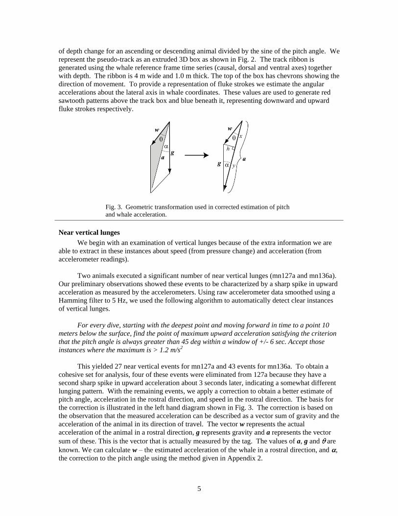
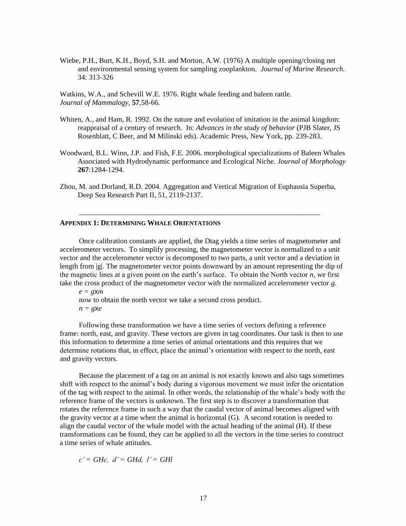
Fig. 3. Geometric transformation used in corrected estimation of pitch

and whale acceleration.

Near vertical lunges

We begin with an examination of vertical lunges because of the extra information we are

able to extract in these instances about speed (from pressure change) and acceleration (from

accelerometer readings).

Two animals executed a significant number of near vertical lunges (mn127a and mn136a).

Our preliminary observations showed these events to be characterized by a sharp spike in upward

acceleration as measured by the accelerometers. Using raw accelerometer data smoothed using a

Hamming filter to 5 Hz, we used the following algorithm to automatically detect clear instances

of vertical lunges.

For every dive, starting with the deepest point and moving forward in time to a point 10

meters below the surface, find the point of maximum upward acceleration satisfying the criterion

that the pitch angle is always greater than 45 deg within a window of +/- 6 sec. Accept those

instances where the maximum is > 1.2 m/s2

This yielded 27 near vertical events for mn127a and 43 events for mn136a. To obtain a

cohesive set for analysis, four of these events were eliminated from 127a because they have a

second sharp spike in upward acceleration about 3 seconds later, indicating a somewhat different

lunging pattern. With the remaining events, we apply a correction to obtain a better estimate of

pitch angle, acceleration in the rostral direction, and speed in the rostral direction. The basis for

the correction is illustrated in the left hand diagram shown in Fig. 3. The correction is based on

the observation that the measured acceleration can be described as a vector sum of gravity and the

acceleration of the animal in its direction of travel. The vector w represents the actual

acceleration of the animal in a rostral direction, g represents gravity and a represents the vector

sum of these. This is the vector that is actually measured by the tag. The values of a, g and are

known. We can calculate w – the estimated acceleration of the whale in a rostral direction, and ,

the correction to the pitch angle using the method given in Appendix 2.

6

The corrected pitch angle p is

p = 90.0 -

Once we have p we can estimate the speed s in a caudal direction.

s = depth/(sin(p) t);

The average speed profiles for the two animals are shown in Fig. 4a. Prior to the lunge the

animals move upward from between 1 and 1.3 m/s. The lunge is characterized by two pulsed

increases in speed. Following the second pulse the speed returns roughly to its previous value.

Figure 4b shows the corrected acceleration in a caudal direction. There is a sharp spike in

acceleration with a peak average value of 2.3 m/sec2. Note that this spike is much larger than that

seen in normal upward swimming and this provides the strongest direct evidence for lunging.

Figure 4c shows the mean variation in pitch angle during the course of an upward lunge.

The other four animals showed many instances of lunging in a generally upward direction,

but only two yielded any upward lunges meeting our criteria: mn122b yielded 2 events and

mn148a yielded 3 events.

Figure. 4. Average speed, acceleration and pitch for two animals. These are centered about a peak in

upward acceleration.

These data show that humpbacks use remarkably few fluke strokes to make a lunge. The

pitch angle plot suggests that the animal may make a single two-way fluke stroke to gain speed,

ending with its flukes hyper-rotated downward. This hyper-rotation likely slows the animal just

prior to the lunge, but it may also facilitate the steering of the body around the buccal cavity to

ensure more rapid closure of the mouth immediately following the lunge. The actual lunge is

accomplished by a single massive upstroke presumably with the mouth open, propelling the

7

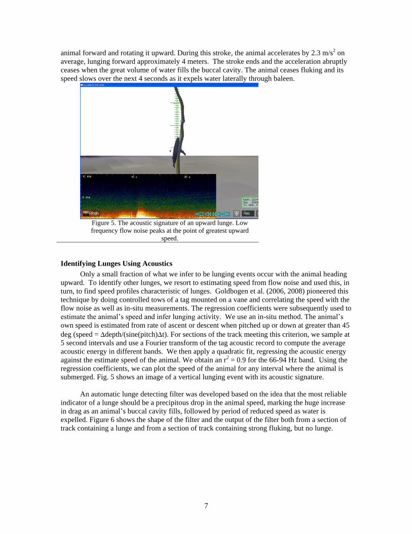
animal forward and rotating it upward. During this stroke, the animal accelerates by 2.3 m/s2 on

average, lunging forward approximately 4 meters. The stroke ends and the acceleration abruptly

ceases when the great volume of water fills the buccal cavity. The animal ceases fluking and its

speed slows over the next 4 seconds as it expels water laterally through baleen.

Figure 5. The acoustic signature of an upward lunge. Low

frequency flow noise peaks at the point of greatest upward

speed.

Identifying Lunges Using Acoustics

Only a small fraction of what we infer to be lunging events occur with the animal heading

upward. To identify other lunges, we resort to estimating speed from flow noise and used this, in

turn, to find speed profiles characteristic of lunges. Goldbogen et al. (2006, 2008) pioneered this

technique by doing controlled tows of a tag mounted on a vane and correlating the speed with the

flow noise as well as in-situ measurements. The regression coefficients were subsequently used to

estimate the animal’s speed and infer lunging activity. We use an in-situ method. The animal’s

own speed is estimated from rate of ascent or descent when pitched up or down at greater than 45

deg (speed = depth/(sine(pitch) t). For sections of the track meeting this criterion, we sample at

5 second intervals and use a Fourier transform of the tag acoustic record to compute the average

acoustic energy in different bands. We then apply a quadratic fit, regressing the acoustic energy

against the estimate speed of the animal. We obtain an r2 = 0.9 for the 66-94 Hz band. Using the

regression coefficients, we can plot the speed of the animal for any interval where the animal is

submerged. Fig. 5 shows an image of a vertical lunging event with its acoustic signature.

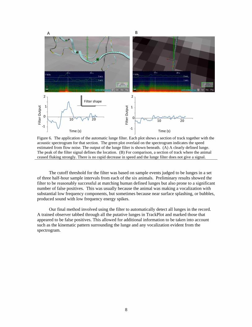
An automatic lunge detecting filter was developed based on the idea that the most reliable

indicator of a lunge should be a precipitous drop in the animal speed, marking the huge increase

in drag as an animal’s buccal cavity fills, followed by period of reduced speed as water is

expelled. Figure 6 shows the shape of the filter and the output of the filter both from a section of

track containing a lunge and from a section of track containing strong fluking, but no lunge.

8

Figure 6. The application of the automatic lunge filter. Each plot shows a section of track together with the

acoustic spectrogram for that section. The green plot overlaid on the spectrogram indicates the speed

estimated from flow noise. The output of the lunge filter is shown beneath. (A) A clearly defined lunge.

The peak of the filter signal defines the location. (B) For comparison, a section of track where the animal

ceased fluking strongly. There is no rapid decrease in speed and the lunge filter does not give a signal.

The cutoff threshold for the filter was based on sample events judged to be lunges in a set

of three half-hour sample intervals from each of the six animals. Preliminary results showed the

filter to be reasonably successful at matching human defined lunges but also prone to a significant

number of false positives. This was usually because the animal was making a vocalization with

substantial low frequency components, but sometimes because near surface splashing, or bubbles,

produced sound with low frequency energy spikes.

Our final method involved using the filter to automatically detect all lunges in the record.

A trained observer tabbed through all the putative lunges in TrackPlot and marked those that

appeared to be false positives. This allowed for additional information to be taken into account

such as the kinematic pattern surrounding the lunge and any vocalization evident from the

spectrogram.

9

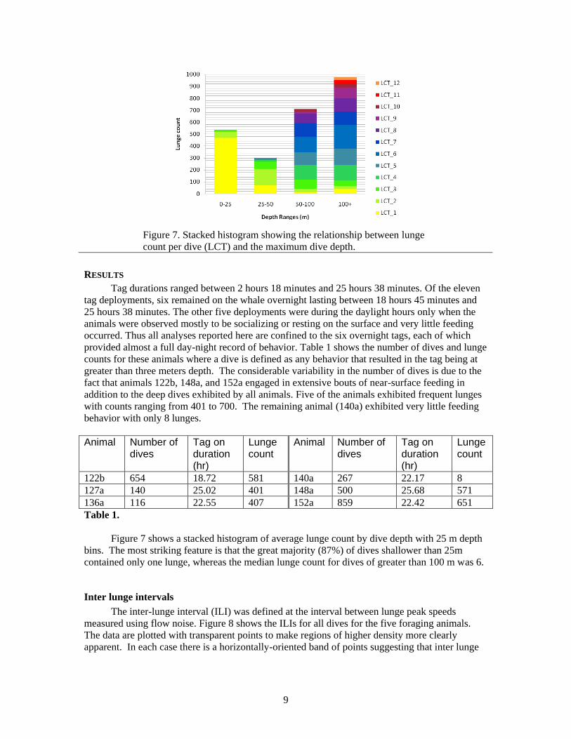
Figure 7. Stacked histogram showing the relationship between lunge

count per dive (LCT) and the maximum dive depth.

RESULTS

Tag durations ranged between 2 hours 18 minutes and 25 hours 38 minutes. Of the eleven

tag deployments, six remained on the whale overnight lasting between 18 hours 45 minutes and

25 hours 38 minutes. The other five deployments were during the daylight hours only when the

animals were observed mostly to be socializing or resting on the surface and very little feeding

occurred. Thus all analyses reported here are confined to the six overnight tags, each of which

provided almost a full day-night record of behavior. Table 1 shows the number of dives and lunge

counts for these animals where a dive is defined as any behavior that resulted in the tag being at

greater than three meters depth. The considerable variability in the number of dives is due to the

fact that animals 122b, 148a, and 152a engaged in extensive bouts of near-surface feeding in

addition to the deep dives exhibited by all animals. Five of the animals exhibited frequent lunges

with counts ranging from 401 to 700. The remaining animal (140a) exhibited very little feeding

behavior with only 8 lunges.

Animal Number of dives

Tag on duration (hr)

Lunge count

Animal Number of dives

Tag on duration (hr)

Lunge count

122b 654 18.72 581 140a 267 22.17 8

127a 140 25.02 401 148a 500 25.68 571

136a 116 22.55 407 152a 859 22.42 651

Table 1.

Figure 7 shows a stacked histogram of average lunge count by dive depth with 25 m depth

bins. The most striking feature is that the great majority (87%) of dives shallower than 25m

contained only one lunge, whereas the median lunge count for dives of greater than 100 m was 6.

Inter lunge intervals

The inter-lunge interval (ILI) was defined at the interval between lunge peak speeds

measured using flow noise. Figure 8 shows the ILIs for all dives for the five foraging animals.

The data are plotted with transparent points to make regions of higher density more clearly

apparent. In each case there is a horizontally-oriented band of points suggesting that inter lunge

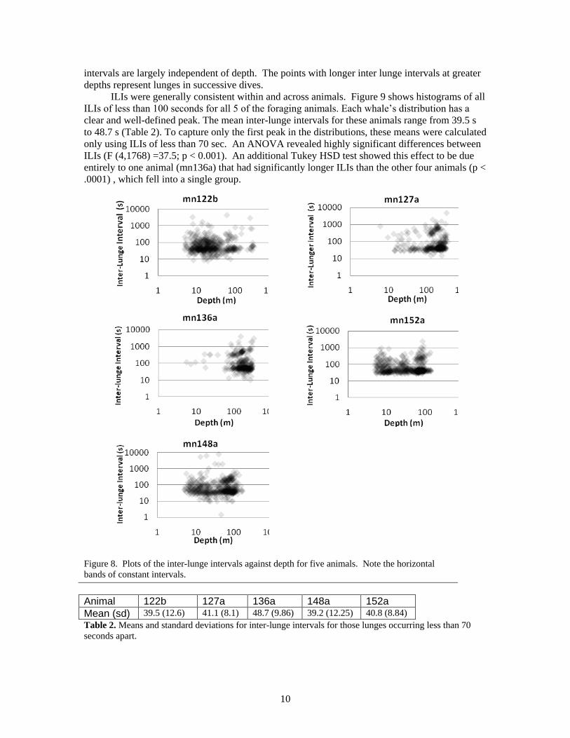
10

intervals are largely independent of depth. The points with longer inter lunge intervals at greater

depths represent lunges in successive dives.

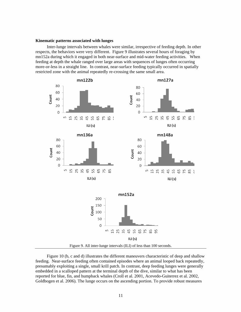
ILIs were generally consistent within and across animals. Figure 9 shows histograms of all

ILIs of less than 100 seconds for all 5 of the foraging animals. Each whale’s distribution has a

clear and well-defined peak. The mean inter-lunge intervals for these animals range from 39.5 s

to 48.7 s (Table 2). To capture only the first peak in the distributions, these means were calculated

only using ILIs of less than 70 sec. An ANOVA revealed highly significant differences between

ILIs (F (4,1768) =37.5; p < 0.001). An additional Tukey HSD test showed this effect to be due

entirely to one animal (mn136a) that had significantly longer ILIs than the other four animals (p <

.0001) , which fell into a single group.

Figure 8. Plots of the inter-lunge intervals against depth for five animals. Note the horizontal

bands of constant intervals.

Animal 122b 127a 136a 148a 152a

Mean (sd) 39.5 (12.6) 41.1 (8.1) 48.7 (9.86) 39.2 (12.25) 40.8 (8.84)

Table 2. Means and standard deviations for inter-lunge intervals for those lunges occurring less than 70

seconds apart.

11

Kinematic patterns associated with lunges

Inter-lunge intervals between whales were similar, irrespective of feeding depth. In other

respects, the behaviors were very different. Figure 9 illustrates several hours of foraging by

mn152a during which it engaged in both near-surface and mid-water feeding activities. When

feeding at depth the whale ranged over large areas with sequences of lunges often occurring

more-or-less in a straight line. In contrast, near-surface feeding typically occurred in spatially

restricted zone with the animal repeatedly re-crossing the same small area.

Figure 9. All inter-lunge intervals (ILI) of less than 100 seconds.

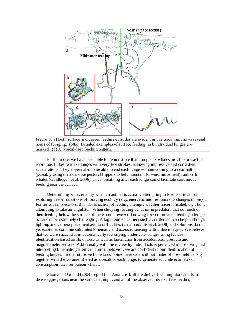
Figure 10 (b, c and d) illustrates the different maneuvers characteristic of deep and shallow

feeding. Near-surface feeding often contained episodes where an animal looped back repeatedly,

presumably exploiting a single, small krill patch. In contrast, deep feeding lunges were generally

embedded in a scalloped pattern at the terminal depth of the dive, similar to what has been

reported for blue, fin, and humpback whales (Croll et al. 2001, Acevedo-Guiterrez et al. 2002,

Goldbogen et al. 2006). The lunge occurs on the ascending portion. To provide robust measures

12

of the differences between the two feeding modes we compared median turn rates for 40 minutes

of deep feeding from animal mn152a with a 40-minute period of surface feeding by the same

animal. The median azimuthal turn rate was 2.86 deg/s for surface feeding compared to 1.28

deg/s for deeper feeding. Median roll rate similarly differed by more than a factor of two (2.79

deg/s versus 1.30 deg/s) and median pitch angle change varied by 57% (4.95 deg/s versus 3.19

deg/s). A CHI squared median test (Siegel, 1956) showed all of these differences to be highly

significant (p < 0.001).

DISCUSSION

When prey is abundant and uniformly dense around a predator, optimal foraging theory

(Charnov 1976) suggests that an animal feeds as frequently as possible in as close proximity to

the initial location as possible. In the case of humpback whales, this would mean prey being

distributed evenly throughout the water column, and optimal foraging would mean feeding

(lunging) as close to the surface and as frequently as possible. The fact that our measured inter-

lunge intervals are consistent for both deep and shallow lunges strongly suggests a biomechanical

limit to the lunge-filter cycle. The inter-lunge intervals we measured were similar to those

previously reported for humpbacks. Goldbogen et al. (2008) separated lunge durations (15.5 s)

and times between consecutive lunges (21.5 s), adding these gives an ILI of 37 s similar to our

overall median ILI of 40.1 s.

Despite the similarity in inter-lung interval for deep and shallow feeding, there were large

differences in other respects. Most notably the number of lunges per dive were very different

with animals executing one lunge per dive for dives of less than 25 meters, one or two lunges per

dive between 25 and 50 m and a median six lunges per dive for dives greater than 100 m. The

finding of one lunge per dive when feeding near the surface, combined with the constant inter-

lunge interval suggests that the animals can integrate respiration into the lunge and filter cycle to

maximize the rate at which they are able to forage. At an average speed of 1.5 m/s an animal can

dive to less than 30 m and back in about 45 seconds consistent with the transition from one to

more lunges per dive that we found between 25 and 50 m. At greater depths it should be more

efficient to execute several lunges per dive followed by multiple breaths on each surfacing.

13

Figure 10 a) Both surface and deeper feeding episodes are evident in this track that shows several

hours of foraging. (b&c) Detailed examples of surface feeding, in b individual lunges are

marked. (d) A typical deep feeding pattern.

Furthermore, we have been able to demonstrate that humpback whales are able to use their

enormous flukes to make lunges with very few strokes, achieving impressive and consistent

accelerations. They appear also to be able to end each lunge without coming to a near halt

(possibly using their oar-like pectoral flippers to help maintain forward movement), unlike fin

whales (Goldbogen et al. 2006). Thus, breathing after each lunge could facilitate continuous

feeding near the surface.

Determining with certainty when an animal is actually attempting to feed is critical for

exploring deeper questions of foraging ecology (e.g., energetic and responses to changes in prey).

For terrestrial predators, this identification of feeding attempts is rather uncomplicated, e.g., lions

attempting to take an ungulate. When studying feeding behavior in predators that do much of

their feeding below the surface of the water, however, knowing for certain when feeding attempts

occur can be extremely challenging. A tag mounted camera such as crittercam can help, although

lighting and camera placement add to difficulties (Calambokidis et al. 2008) and solutions do not

yet exist that combine calibrated kinematic and acoustic sensing with video imagery. We believe

that we were successful in automatically identifying underwater lunges using feature

identification based on flow noise as well as kinematics from accelometer, pressure and

magnetometer sensors. Additionally with the review by individuals experienced in observing and

interpreting kinematic patterns in animal behavior, we are confident in our identification of

feeding lunges. In the future we hope to combine these data with estimates of prey field density

together with the volume filtered as a result of each lunge, to generate accurate estimates of

consumption rates for baleen whales.

Zhou and Dorland (2004) report that Antarctic krill are diel vertical migrators and form

dense aggregations near the surface at night, and all of the observed near-surface feeding

14

behavior in this study occurred at night. It seems likely that the distribution and abundance of

prey near the surface was both patchy and dense, which may account for the much greater rate of

turning for increased foraging attempts on prey near the surface compared to deeper feeding. A

fascinating strategy utilized by multiple whales was a stereotyped reverse-looping near the

surface, during which the whales looped back to lunge through the same area repeatedly (Figure

9). This looping behavior would allow the whales to either exploit or to corral and then exploit a

small and very dense prey patch, or perhaps this behavior is a combination of the two. These

unique feeding behaviors may be the result of some type of learning based on repeated

interactions with the same prey item throughout the lifetime of an individual (e.g., trial-and-error

or observational (see Whiten and Hamm 1992 for a review of learning strategies)).

Our results provide novel information regarding the underwater foraging behaviors and

kinematics of humpback whales. Because of the near vertical lunges exhibited by two animals in

particular we have been able to obtain direct measurements of accelerations and speeds (from

pressure change) during underwater lunge feeding events and apply this to other whales that

employ lunge-based feeding regardless of their body orientation. This information can be used to

compare and contrast differences between baleen whale species within and across geographic

regions to better understand predator-prey interactions and the ecological role of cetaceans. Our

results also show that humpback whales are able to generate the speed necessary for lunging

quicker than other baleen whale species and that they do not slow to a near halt following a lunge.

It is worth noting that we found flow noise to be a very unreliable determinant of speed below

about 0.8 m/s, thus our use of the near vertical lunges as initial exemplars in our analyses, based

on the assumption that horizontal and vertical lunges have the same kinematic form. We must

qualify our interpretations of pure acceleration, however, because the tags are not placed at the

animal’s center of mass. We are in fact measuring at a point that is usually roughly midway

between the blowhole and the dorsal fin. Undoubtedly a component of the values we measure

comes from the flexing of the animal’s body, although in the absence of additional

instrumentation we are unable to resolve the various contributions. In the future tags that

incorporate gyros can provide a reference frame enabling accelerations in any direction to be

measured (Martin et al. 2005).

ACKNOWLEDGEMENTS

We are grateful to Reny Tyson for her careful review of the entire set of lunges and to

Alison Stimpert and the rest of the MISHAP tag team for the tag deployment effort. The

TrackPlot processing package would not have been developed without the enthusiastic support

and contributing ideas of David Wiley. Funding for TrackPlot development was provided by an

ONR grant to Colin Ware (ONR N0014091601). We are grateful to the ship and technical crews

of the ASRV LM Gould. This work was supported by NSF Polar Programs Award ANT-07-

39483. This research was conducted under NMFS MMPA Permit 808-1735 and Antarctic

Conservation Act permit 2009-014.

LITERATURE CITED

Acevedo-Guiterrez, A., Croll, D.A., Tershy, B.R. 2002. High feeding costs limit dive time in the

largest whales. Journal of Experimental Biology, 205:1747-1753

Brodie, P.F. 1977. Form, function and energetics of cetacea: A discussion. In Functional

Anatomy of Marine Mammals. Vol. 3. Ed. R.J. Harrison. Academic Press, New York,

pp.45-56.

15

Brodie, P.F. 1993. Noise generated by the jaw actions of feeding fin whales. Can. J. Zool.

71:2546-2550.

Croll, D.A., Acevedo-Guitierrez, A, Tershy BR, Urban-Ramirez J. 2001. The diving behavior of

blue and fin whales: is dive duration shorter than expected based on oxygen stores.

Comparative Biochemistry and Physiology Part A 129:797-809

Calambokidis, J., Schorr, G.S., Steiger, G.H., Francis, J., Bakhtirai, M., Marshall, G. and Oleson,

E., Gendron, D. and Robertson, K. 2008. Insights into the underwater diving, feeding and

calling behavior of blue whales from a suction-cup attached video-imaging tag (crittercam).

Marine Technology Society Journal, 41(4):19-29.

Charnov, E.L. 1976, Optimal foraging, the marginal value theorem. Theoretical Populatino

Biology, 9: 129-136.

Demer, D.A. and Conti, S.G. 2005. Validation of stochastic distorted-wave Born Approximation

with broad bandwidth total target strength measurement of Antarctic krill. ICES Journal of

Marine Science, 60(3): 625-635.

Dolphin, W.F. 1987. Prey densities and foraging of humpback whales, Megaptera Novaeangliae.

Experientia, 43: 468-471.

Friedlaender, A.S., Hazen, E.L., Nowacek, D.P, Halpin, P.N., Ware, C., Weinrich, M.T.,

Hurst, T., and Wiley, D. 2009. Diel changes in humpback whale Megaptera

novaeangliae feeding behavior in response to sand lance Ammodytes spp. behavior

and distribution. Marine Ecology Progress Series. doi: 10.3354/meps08003

Golbogen, J.A., Calambokidis, J., Croll, D.A., Harvey, J.T., Newton, K.M., Oleson, E.M., Schorr,

G., and Shadwick, R.E. 2008. Foraging behavior of humpback whales: kimematic and

respiratory patterns suggest a high cost for a lunge. Journal of Experimental Biology,

211:3712-3719.

Golbogen, J.A., Pyenson, N.D., and Shadwick, R.E. 2007, Big gulps require high drag for fin

whale lunge feeding. Marine Ecology Progress Series. 343: 289-301.

Goldbogen, J.A., Calambokidis, J., Shadwick, R.E., Oleson, E.M., McDonald, M.A., and

Hildebrand, J.A. 2006. Kinematics of foraging dives and lunge-feeding in fin whales.

Journal of Experimental Biology 209: 1231-1244.

Goldbogen, J. A., Potvin, J., Shadwick, R.E. (2010). Skull and buccal cavity allometry increase

mass-specific engulfment capacity in fin whales. Proceedings of the Royal Society – B

Biological Sciences 277:861-868.

Hain, J.H.W., Ellis, S.L., Kenney, R.D., Clapham, P.J., Gray, B.K., Weinrich, M.T., Babb, I.G.

1995. apparent bottom feeding by humpback whales on Stellwagen Bank. Marine Mammal

Science 11:464-479.

Hain, J.H.W., Carter,G.R. Kraus, S.D. Mayo, C.A. andWinn, H.E. 1982. Feeding behavior of

the humpback whale, Megaptera Noveangliae, in the Western North Atlantic. Fishery

Bulletin 80: 259-268.

16

Hazen, E.L., Friedlaender, A.S., Thompson, M.A., Ware, C.R., Weinrich, M.T., Halpin, P.N., and

Wiley, D.N. 2009. Fine-scale prey aggregations and foraging ecology of humpback whales

(Megaptera novaeangliae). Marine Ecology Progress Series doi:10.3354/meps08108

Johnson, M. and Tyack, P. L. 2003. A digital acoustic recording tag for measuring the response of

wild marine mammals to sound. IEEE Journal of Oceanic Engineering, 28, 3-12.

Johnston, D.W., Friedlaender, A.S., Read, A.J., and Nowacek, D.P. in review. Density estimates

of humpback whales (megaptera novaeangliae) in the inshore waters of the Western

Antarctic Peninsula during the late autumn. Endangered Species Research.

Jurasz, C.M., and Jurasz, V.P. 1979. Feeding modes of the humpback whale Megaptera

Novaeangliage, in Southeast Alaska. Scientific Reports of the Whales Research Institute

31:67-81.

Kot, B. W. 2005. Rorqual whale surface-feeding strategies: biomechanical aspects of

feeding anatomy and exploitation of prey aggregations along tidal fronts. M.Sc.

thesis, University of California, Los Angeles.

Lambertsen, R., Ulrich, N. and Straley, J. 1995. Frontomandibular Stay of Balaenopteridae: a

Mechanism for Momentum recapture during feeding. Journal of Mammalogy 76(3):877-

899.

Matthews, L. H. 1937. The humpback whale, Megaptera nodosa. Discovery Reports 17:7-92.

Nowacek, D.P. 2002. Sequential foraging behaviour of bottlenose dolphins, Tursiops truncatus,

in Sarasota Bay, FL. Behaviour, 139 (9): 1125-1145.

O’Brien, D.P. (987. Description of escape responses of krill (Crustacea: Euphausiacea), with

particular reference to swarming behavior and the size and proximity of the predator.

Journal of Crustacean Biology, 7(3): 449-457.

Orton, L.S., and Brodie, P.F. 1987. Engulfing mechanics of fin whales. Canadian Journal of

Zoology 65:2898-2907.

Pivorunas, A. 1979 The feeding mechanisms of baleen whales. American Scientist 67: 432-440.

Potvin, J. Goldbogen, J.A., and Shadwick, R.E., 2009. Passive versus active engulfment: verdict

from trajectory simulations of lunge-feeding fin whales Balaenoptera physalus. Journal of

the Royal Society Interface 6: 1005–1025.

Seigel, S. (1956) Nonparametric Statistics for the Behavioral Sciences. McGraw Hill, Toronto.

Sharpe, F.A. 2001. Social Foraging of the Southeast Alaskan Humpback Whale, Megaptera

novaeangliae. PhD Dissertation, Simon Fraser University, Vancouver, British Columbia,

Canada.

Ware, C., Arsenault, R., Wiley, D. Plumlee, M. 2006. Visualizing the underwater behavior of

humpback whales. IEEE Computer Graphics and Applications, 14-18.

17

Wiebe, P.H., Burt, K.H., Boyd, S.H. and Morton, A.W. (1976) A multiple opening/closing net

and environmental sensing system for sampling zooplankton. Journal of Marine Research.

34: 313-326

Watkins, W.A., and Schevill W.E. 1976. Right whale feeding and baleen rattle.

Journal of Mammalogy, 57,58-66.

Whiten, A., and Ham, R. 1992. On the nature and evolution of imitation in the animal kingdom:

reappraisal of a century of research. In: Advances in the study of behavior (PJB Slater, JS

Rosenblatt, C Beer, and M Milinski eds). Academic Press, New York, pp. 239-283.

Woodward, B.L. Winn, J.P. and Fish, F.E. 2006. morphological specializations of Baleen Whales

Associated with Hydrodynamic performance and Ecological Niche. Journal of Morphology

267:1284-1294.

Zhou, M. and Dorland, R.D. 2004. Aggregation and Vertical Migration of Euphausia Superba,

Deep Sea Research Part II, 51, 2119-2137.

__________________________________________________________________

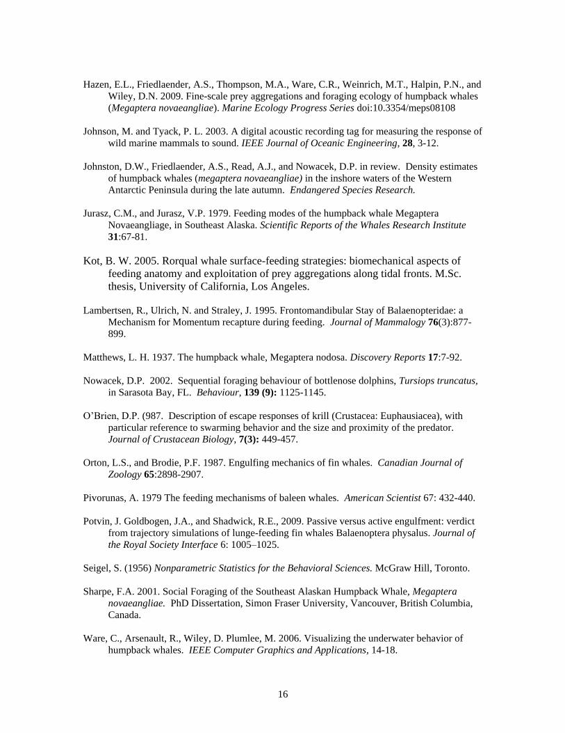
APPENDIX 1: DETERMINING WHALE ORIENTATIONS

Once calibration constants are applied, the Dtag yields a time series of magnetometer and

accelerometer vectors. To simplify processing, the magnetometer vector is normalized to a unit

vector and the accelerometer vector is decomposed to two parts, a unit vector and a deviation in

length from |g|. The magnetometer vector points downward by an amount representing the dip of

the magnetic lines at a given point on the earth’s surface. To obtain the North vector n, we first

take the cross product of the magnetometer vector with the normalized accelerometer vector g.

e = gxm

now to obtain the north vector we take a second cross product.

n = gxe

Following these transformation we have a time series of vectors defining a reference

frame: north, east, and gravity. These vectors are given in tag coordinates. Our task is then to use

this information to determine a time series of animal orientations and this requires that we

determine rotations that, in effect, place the animal’s orientation with respect to the north, east

and gravity vectors.

Because the placement of a tag on an animal is not exactly known and also tags sometimes

shift with respect to the animal’s body during a vigorous movement we must infer the orientation

of the tag with respect to the animal. In other words, the relationship of the whale’s body with the

reference frame of the vectors is unknown. The first step is to discover a transformation that

rotates the reference frame in such a way that the caudal vector of animal becomes aligned with

the gravity vector at a time when the animal is horizontal (G). A second rotation is needed to

align the caudal vector of the whale model with the actual heading of the animal (H). If these

transformations can be found, they can be applied to all the vectors in the time series to construct

a time series of whale attitudes.

c’ = GHc, d’ = GHd, l’ = GHl

18

By aligning the accelerometer vector with the down direction and the orthogonal

component of the magnetometer vector with north, a time series of tag orientations can be

produced.

TrackPlot uses the following method to determine this transformation. First a short section

to track is identified where the animal is presumed to be swimming horizontally. This section is

marked and TrackPlot averages the acceleration vectors over the interval. TrackPlot then

calculates the rotation matrix needed to rotate the ventral vector of the whale model to match the

gravity vector. All that is needed is a second rotation to bring the caudal vector into alignment

with the actual heading of the animal. To accomplish this step the animal proxy is moved along

the track to where there is a steep ascent or descent. The user can then manually rotate a

representation of the whale’s reference frame so that the caudal vector is pointing down. This

rotation is encoded as an azimuth rotation matrix R. TrackPlot generates a time series of vectors

representing the caudal, dorsal, and lateral vectors in world coordinates. The non-georeferenced

pseudo-track ribbon is constructed by assuming that the animal is progressing forward at a

constant speed of 1 m/s with the exception that when the animal is pitched up or down by more

than 30 degrees, the change in depth (from pressure) is used to estimate speed through the water

so that

speed = depth /sine(pitch).

__________________________________________________________________

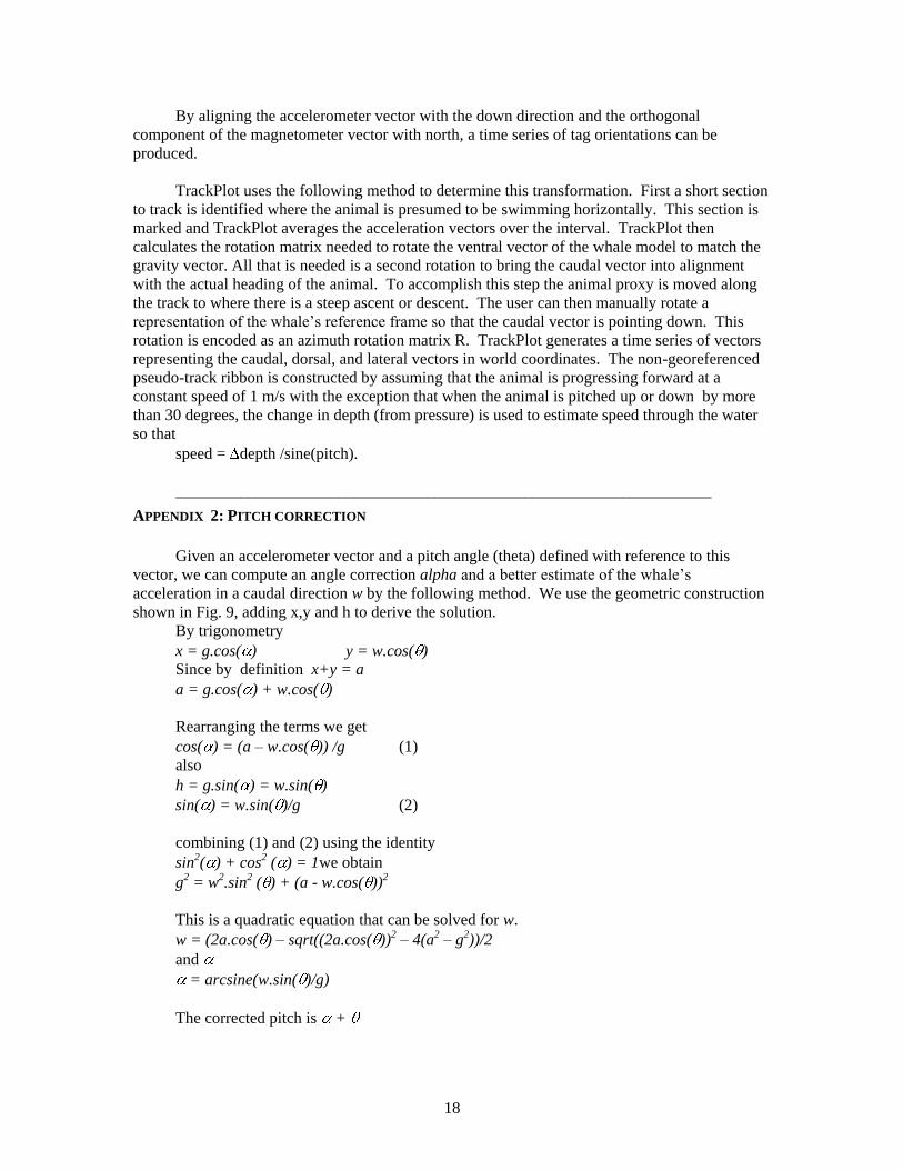
APPENDIX 2: PITCH CORRECTION

Given an accelerometer vector and a pitch angle (theta) defined with reference to this

vector, we can compute an angle correction alpha and a better estimate of the whale’s

acceleration in a caudal direction w by the following method. We use the geometric construction

shown in Fig. 9, adding x,y and h to derive the solution.

By trigonometry

x = g.cos( ) y = w.cos( )

Since by definition x+y = a

a = g.cos( ) + w.cos( )

Rearranging the terms we get

cos( ) = (a – w.cos( )) /g (1)

also

h = g.sin( ) = w.sin( )

sin( ) = w.sin( )/g (2)

combining (1) and (2) using the identity

sin2( ) + cos2 ( ) = 1we obtain

g2 = w2.sin2 ( ) + (a - w.cos( ))2

This is a quadratic equation that can be solved for w.

w = (2a.cos( ) – sqrt((2a.cos( ))2 – 4(a2 – g2))/2

and

= arcsine(w.sin( )/g)

The corrected pitch is +