AD-A237 976 7 &

Shallow Water RASP Upgrade

. JU., .i / 991 '

J. K. FulfordNumerical Modeling DivisionOcean Acoustics and Technology Directorate

Approved for public release; distribution is unlimited. NavalOceanographic and Atmospheric Research Laboratory, Stennis SpaceCenter, Mississippi 39529-5004.

91-03554,4IIII Ull! 11111 111) ll

These working papers were prepared for the timelydissemination of information; this document doesnot represent the official position of NOARL.

ABSTRACT

The Range Dependent Active System Performance model (RASP) has beenmodified to function at higher frequencies in shallower water than itsinitial design specification. The major difficulties in the original versionof the model were the control of the cubic spline fitting routines to thesound speed points, extension of attenuation coefficients to higherfrequencies and the need to interface to Navy standard data bases (ormodels) for bottom loss calculations. These two areas of difficulty wereovercome using a front end sound speed fitting algorithm based on cubicsplines under tension to control the oscillations in the spline fits in themodel, and subroutines to allow input of standard bottom loss curves.

The resulting modifications to the model created a model capable ofpredicting range dependent monostatic reverberation (with reasonableaccuracy) at frequencies up to 10 kHz. The modifications did not addressthe broader problem of bistatic range dependent reverberation at highfrequencies (or in shallow water), or the problem of "energy splittingloss" on predicted target returns.

-l".. . ..V T ). B

IL1.t __, __ __ i _/_

'Diet

ACKNOWLEDGMENTS

This work was supported by the ASW Environmental Acoustics Support(AEAS) division (code 124 A), Program Element 0603785N, Dr. E. EstalotteJr., Program Manager. The data used to verify the modeling modificationswere provided by B. Davis at NAVAIR PMA 264 and J. Gottwald of G/JAssociates.

ii

CONTENTS

INTRODUCTION 1

SOUND SPEED FITTING MODIFICATION 1

ATTENUATION FUNCTION 2

BOTTOM LOSS 3

SAMPLE RESULTS 3

SUMMARY 7

REFERENCES 9

APPENDIX A A-1

APPENDIX B B-1

iii

Shallow Water Range Dependent Active System Model

(RASP) Upgrade

INTRODUCTION

The requirement to improve active systems modeling capability inshallow water presents a new set of challenge to the active systemmodels that are currently in use. In this technical note the modificationsthat have been made to the Range Dependent Active System Performancemodel (RASP) will be documented. For technical details on the RASP modelthe reader is referred to Franchi et al. (1984).

Primarily the modifications are made to increase the maximumfrequency at which the model can be operated by modifying theattenuation coefficient to be correct at higher frequencies, and byintroducing the High Frequency Bottom Loss (HFBL) curves into the model.Another critical area of modification was to introduce a method thatwould limit the size of extraneous inflection points in the sound speedprofile used by the ray tracing model.

SOUND SPEED FITTING MODIFICATION

RASP converts pairs of depth, velocity to continuous functions via thetechnique of cubic spline (Cornyn, 1973). The cubic spline functionproduces the smoothest interpolant to a set of points that pass throughthe points in the sense that the strain energy associated with the curve isminimized (de Boor, 1978). It does however, produce extra minima andmaxima by failing to preserve the convexity of the set.

There are two approaches that could have been taken to overcome thisproblem. The first approach is to change the fitting routine in the model toone which is more robust with respect to extraneous inflection points. Thesecond approach is to modify the input profiles such that the extraneousinflection points are minimized. The second approach was selected,primarily to minimize the amount of time necessary to introduce the

change.

The cubic spline under tension (Cline, 1974) produces a fitted curve that

maintains the original convexity of the set. Therefore, the input sound

speed profiles were fitted using a cubic spline under tension, andresampled for subsequent entry into the RASP model. It was found that if

the original points were retained along with the densest possible sample,that the extraneous inflections were reduced to a point where their effecton calculations were minimized.

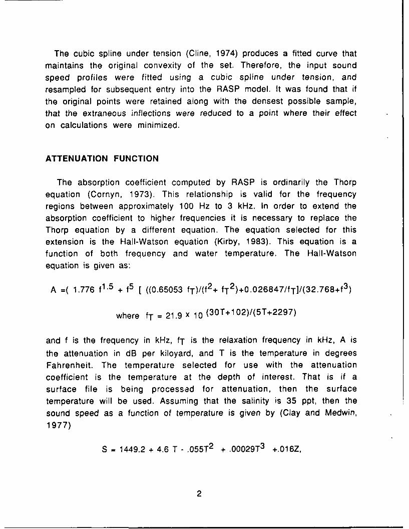
ATTENUATION FUNCTION

The absorption coefficient computed by RASP is ordinarily the Thorp

equation (Cornyn, 1973). This relationship is valid for the frequencyregions between approximately 100 Hz to 3 kHz. In order to extend the

absorption coefficient to higher frequencies it is necessary to replace theThorp equation by a different equation. The equation selected for this

extension is the Hall-Watson equation (Kirby, 1983). This equation is afunction of both frequency and water temperature. The Hall-Watsonequation is given as:

A =( 1.776 fl.5 + f5 [ ((0.65053 fT)/(f2+ fT 2 )+0.026847/fT]/(32.768+f 3 )

where fT = 21.9 x 10 (30T+102)/(5T+2297)

and f is the frequency in kHz, fT is the relaxation frequency in kHz, A is

the attenuation in dB per kiloyard, and T is the temperature in degreesFahrenheit. The temperature selected for use with the attenuation

coefficient is the temperature at the depth of interest. That is if asurface file is being processed for attenuation, then the surfacetemperature will be used. Assuming that the salinity is 35 ppt, then the

sound speed as a function of temperature is given by (Clay and Medwin,1977)

S = 1449.2 + 4.6 T - .055T2 + .00029T 3 +.016Z,

2

where S is the sound speed in m/sec, T is the temperature in degrees

Centigrade, and Z is the depth in meters. For a given depth this formulacan be solved for the temperature that gives the sound speed observed, andthat temperature converted by the well known conversion formula.

BOTTOM LOSS

RASP requires that bottom loss information must be in the form of

bottom loss versus grazing angle. There are two standard methods of

specifying bottom loss. These are the Low Frequency Bottom Loss (LFBL)parameters, and the HFBL curves. The LFBL parameters are usuallyconverted into bottom loss versus grazing angle using the PREP-PEprogram, or some similar program that implements the conversion.Therefore, it must be assumed that the user has access to these routines.The HFBL curves have been implemented via a series of common blocksthat hold the coefficients for the curves, and a query to the user for theprovince for which the bottom loss must be known. This change isreflected in the annotated list of RASP input question presented inappendix A, and some recommended input values in appendix B.

SAMPLE RESULTS

In this section the results of modeling the reverberation at four shallow

water sites will be presented. At each site the results of a single

frequency band is presented.The first site presented is taken from Urick (1969). The water depth is

assumed to be constant 200 ft, with a source depth of 60 ft, and areceiver depth of 80 ft. The source is a SUS Mark 61. The sound speedprofile as extracted from the measurements is given by:

Depth (ft) Sound Speed (ftlsec)0 5051

120 5053200 5011

3

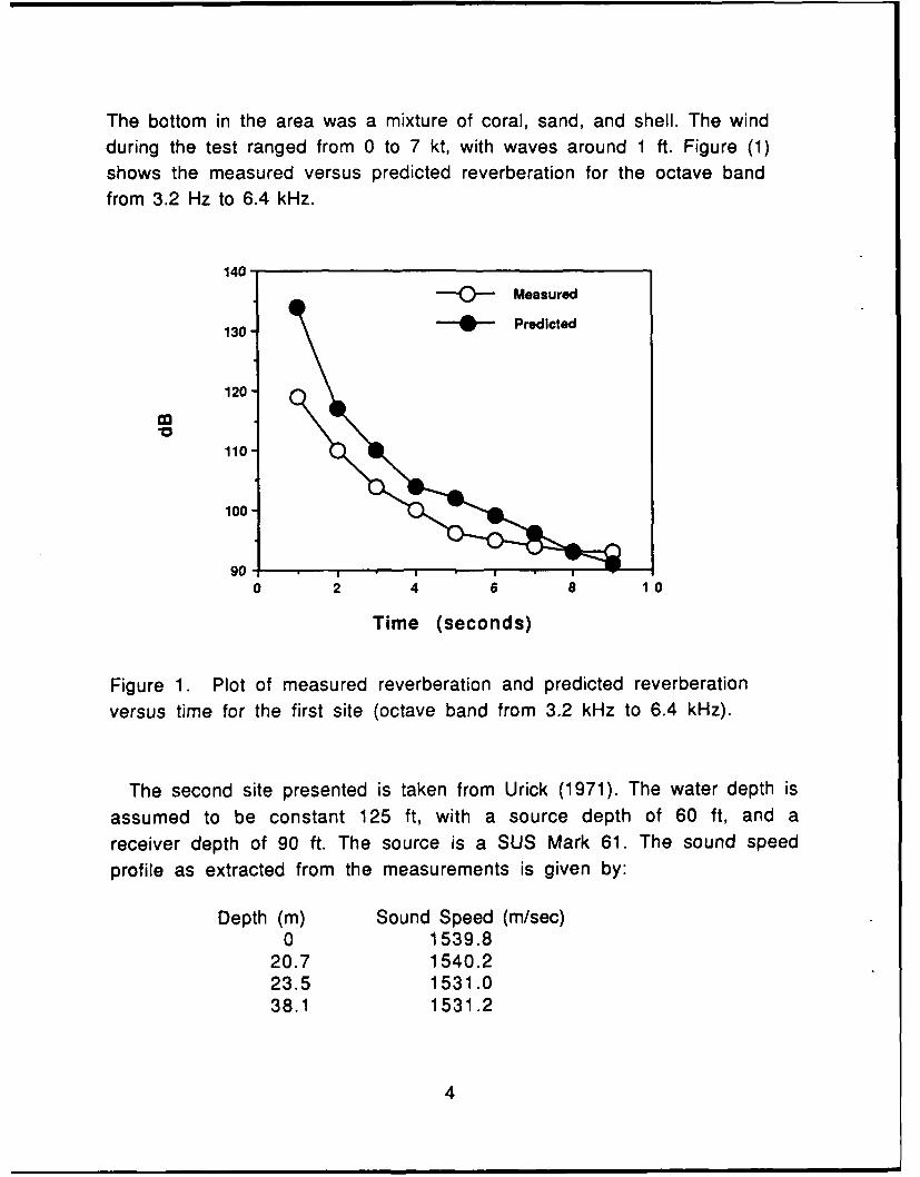
The bottom in the area was a mixture of coral, sand, and shell. The windduring the test ranged from 0 to 7 kt, with waves around 1 ft. Figure (1)shows the measured versus predicted reverberation for the octave bandfrom 3.2 Hz to 6.4 kHz.

140

- Measured

130 - Predicted

120

COV

110

100

900 2 4 6 8 10

Time (seconds)

Figure 1. Plot of measured reverberation and predicted reverberationversus time for the first site (octave band from 3.2 kHz to 6.4 kHz).

The second site presented is taken from Urick (1971). The water depth is

assumed to be constant 125 ft, with a source depth of 60 ft, and a

receiver depth of 90 ft. The source is a SUS Mark 61. The sound speedprofile as extracted from the measurements is given by:

Depth (m) Sound Speed (m/sec)0 1539.8

20.7 1540.223.5 1531.038.1 1531.2

4

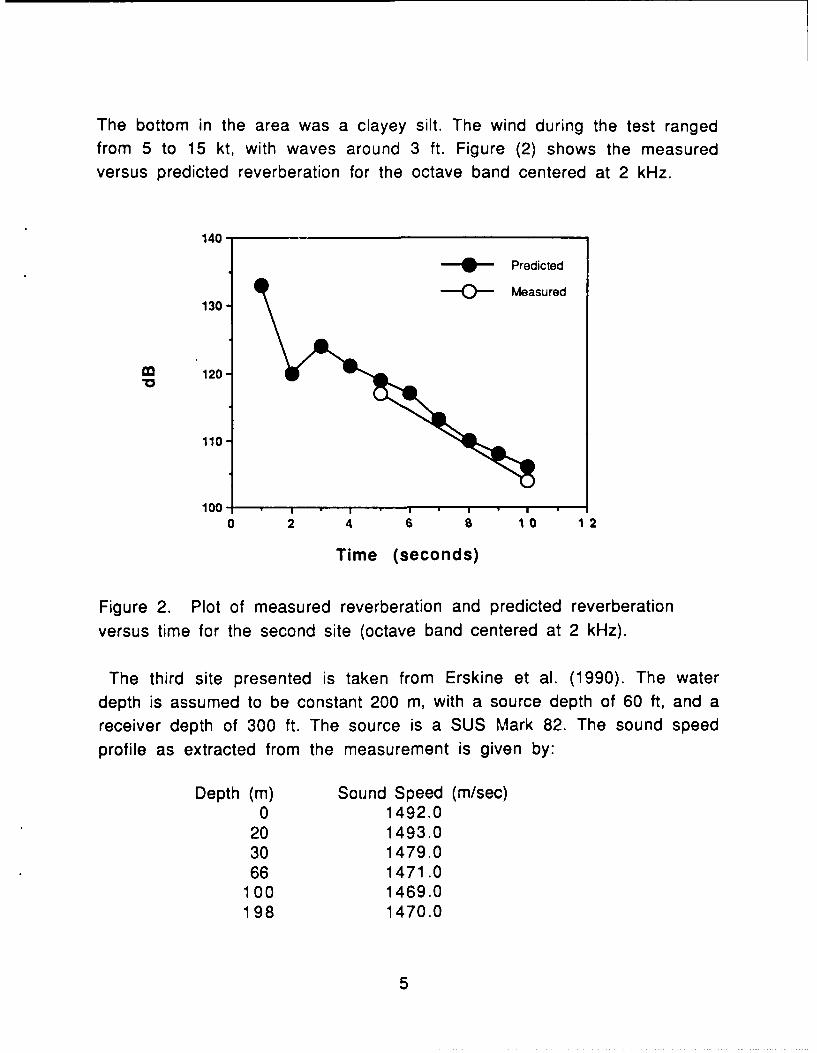
The bottom in the area was a clayey silt. The wind during the test rangedfrom 5 to 15 kt, with waves around 3 ft. Figure (2) shows the measuredversus predicted reverberation for the octave band centered at 2 kHz.

140

- Predicted

-C0- Measured130

120

110

100 -, I , , ,0 2 4 6 a 10 12

Time (seconds)

Figure 2. Plot of measured reverberation and predicted reverberationversus time for the second site (octave band centered at 2 kHz).

The third site presented is taken from Erskine et al. (1990). The waterdepth is assumed to be constant 200 m, with a source depth of 60 ft, and areceiver depth of 300 ft. The source is a SUS Mark 82. The sound speedprofile as extracted from the measurement is given by:

Depth (m) Sound Speed (m/sec)0 1492.0

20 1493.030 1479.066 1471.0

100 1469.0198 1470.0

5

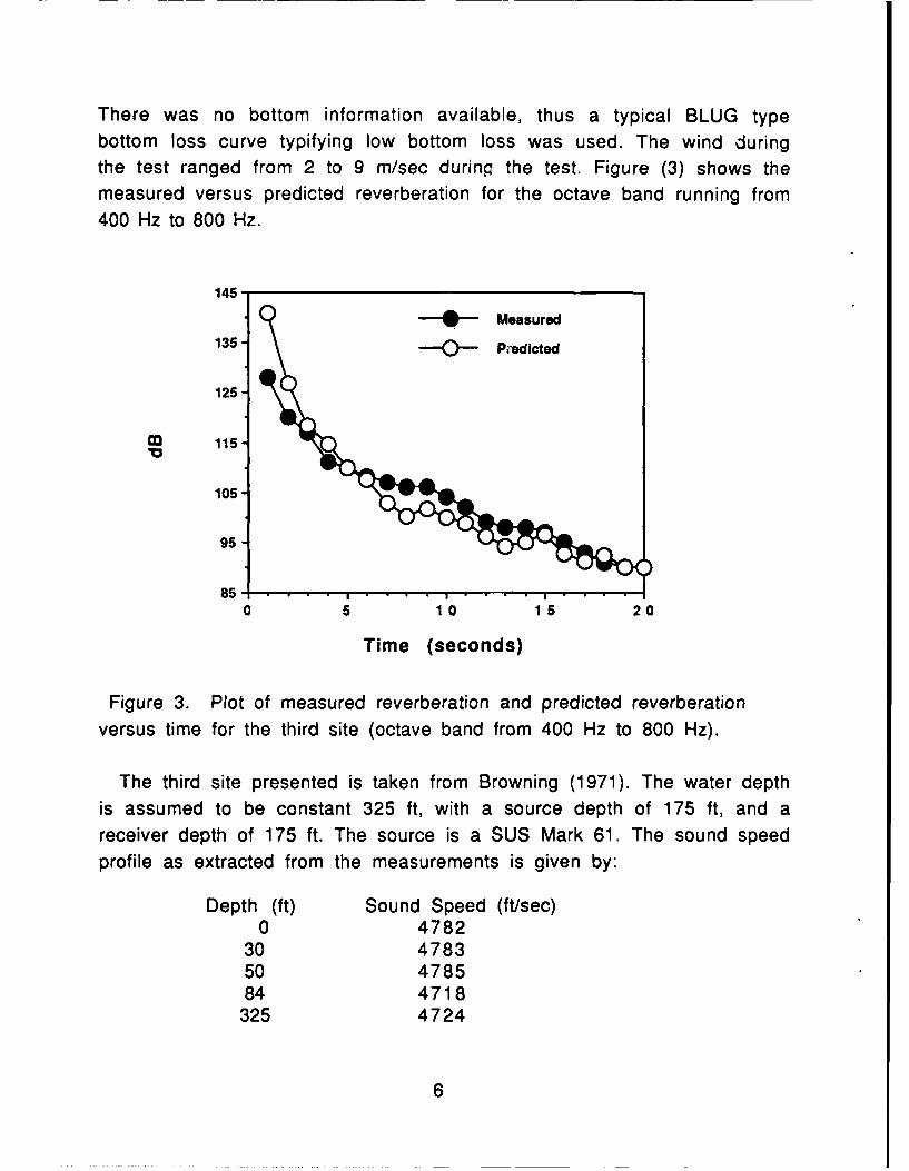
There was no bottom information available, thus a typical BLUG typebottom loss curve typifying low bottom loss was used. The wind duringthe test ranged from 2 to 9 m/sec during the test. Figure (3) shows themeasured versus predicted reverberation for the octave band running from400 Hz to 800 Hz.

145

-Measured135 - Predicted

125

CO 115

105

95

85

0 5 10 15 20

Time (seconds)

Figure 3. Plot of measured reverberation and predicted reverberationversus time for the third site (octave band from 400 Hz to 800 Hz).

The third site presented is taken from Browning (1971). The water depthis assumed to be constant 325 ft, with a source depth of 175 ft, and areceiver depth of 175 ft. The source is a SUS Mark 61. The sound speedprofile as extracted from the measurements is given by:

Depth (ft) Sound Speed (ft/sec)0 4782

30 478350 478584 4718

325 4724

6

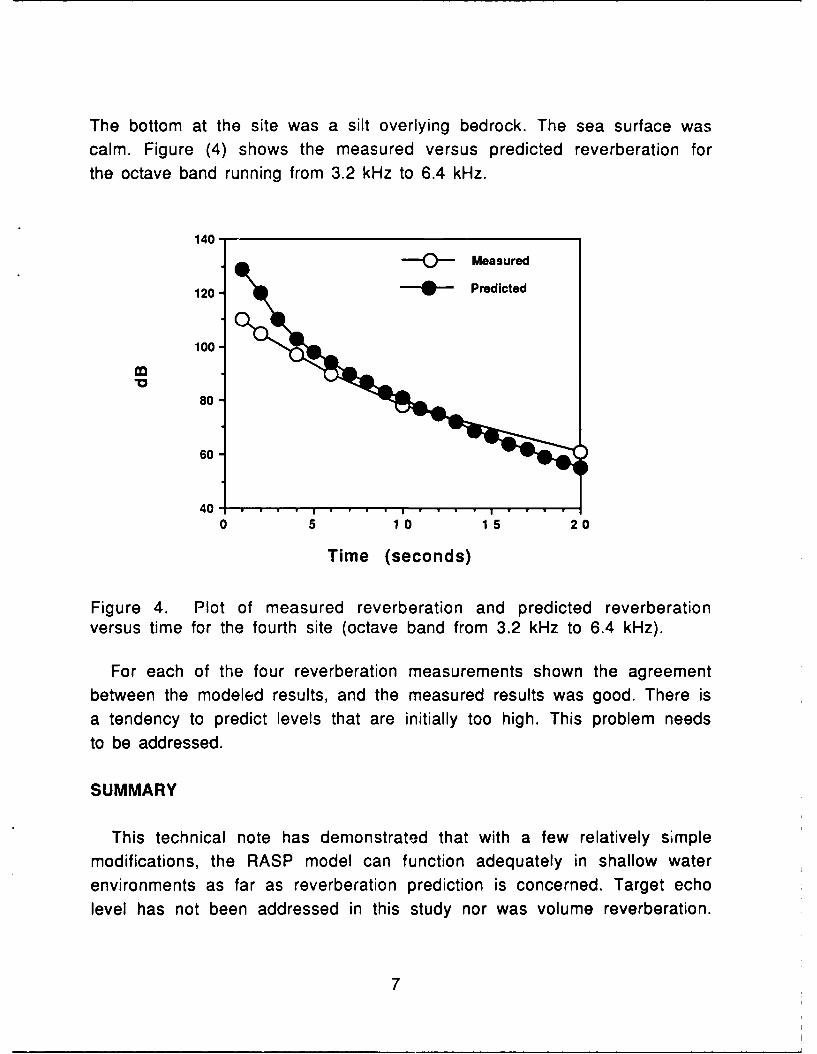
The bottom at the site was a silt overlying bedrock. The sea surface wascalm. Figure (4) shows the measured versus predicted reverberation forthe octave band running from 3.2 kHz to 6.4 kHz.

140-

0 Measured

120 - Predicted

100

80

60-

40O

0 5 10 15 20

Time (seconds)

Figure 4. Plot of measured reverberation and predicted reverberationversus time for the fourth site (octave band from 3.2 kHz to 6.4 kHz).

For each of the four reverberation measurements shown the agreement

between the modeled results, and the measured results was good. There isa tendency to predict levels that are initially too high. This problem needsto be addressed.

SUMMARY

This technical note has demonstrated that with a few relatively simplemodifications, the RASP model can function adequately in shallow water

environments as far as reverberation prediction is concerned. Target echolevel has not been addressed in this study nor was volume reverberation.

7

Volume reverberation was addressed for lower frequencies for CST.Results from studies on modeling active systems in shallow water (Belland Fisch, 1990) reveal that it may be necessary to either include a lossmechanism for energy splitting due to multipath returns, or to calculatethe target returns based on multipath (rather than two way transmissionloss) method.

8

REFERENCES

Browning, David G. (1971). Project CANUS: Sound Propagation andReverberation Measurements in Hudson Bay. Naval Underwater SystemsCenter, New London, CT NUSC Report 4221.

Bell, Thaddeus G. and Norbert P. Fisch (1990). Modeling Signal-ProcessingDegradation for AN/SQQ-891 Active-Sonar Operations in Shallow WaterFinal Report on Baseline Results. Prepared for SPAWAR 315.

Clay, Clarence S. and Herman Medwin (1977). Acoustical OceanographyPrinciples & Applications. Wiley Interscience Publications, 544 pp.

Cline, A. (1974). Scalar- and planar-valued curve fitting using splinesunder tension. Comm. ACM, 17 218-223.

Cornyn, John J. (1973). Grass: A Digital-Computer Ray-Tracing andTransmission-Loss-Prediction System. Naval Research Laboratory,Washington, DC, NRL Report 7621.

de Boor, Carl (1978). A Practical Guide to Splines. Applied MathematicalSeries NO. 27, Springer Verlag, 392 pp.

Erskine, F.T., J.M. Berksen, and P.M. Ogden (1990). Airborne AcousticMeasurments in Shallow Water. Naval Research Laboratory, Washington,DC, NRL Report 9286 (DRAFT).

Franchi, E.R., J.M. Griffin, and B.J. King (1984). NRL Reverberation Model: AComputer Program for the Prediction and Analysis of Medium- to Long-Range Boundary Reverberation. Naval Research Laboratory, Washington, DC,NRL Report 8721.

Kirby, W.D. (1983). Technical Description For the Ship Helicopter AcousticRange Prediction System (Sharps Ill). SAI 83-1011-WA.

9

Urick, R.J. (1969). Acoustic Observations At A Shallow Water Location OffThe Coast Of Florida. Naval Ordnance Laboratory, Silver Spring, MD, NOLTR69-90.

Urick, R.J. (1971). Airborne Measurements Of Shallow Water Acoustics AtVarious Shallow Water Locations Off The Eastern And Gulf Coasts Of TheUnited States. Naval Ordnance Laboratory, Silver Spring, MD, NOLTR 71-4.

10

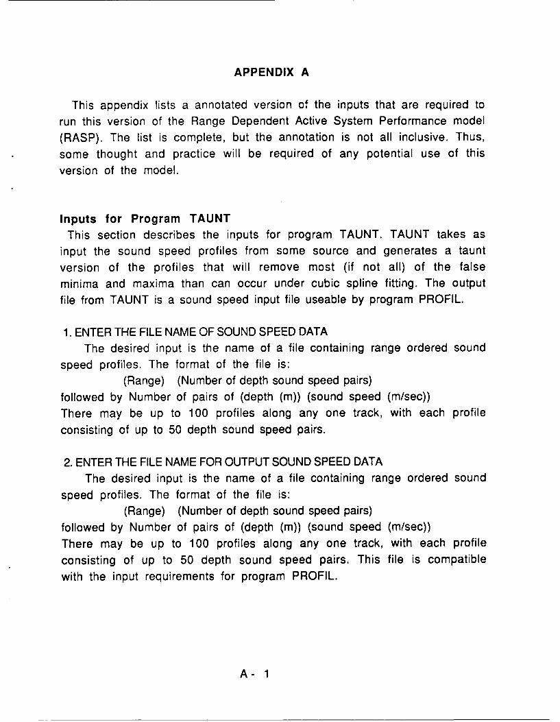
APPENDIX A

This appendix lists a annotated version of the inputs that are required to

run this version of the Range Dependent Active System Performance model

(RASP). The list is complete, but the annotation is not all inclusive. Thus,

some thought and practice will be required of any potential use of this

version of the model.

Inputs for Program TAUNTThis section describes the inputs for program TAUNT. TAUNT takes as

input the sound speed profiles from some source and generates a taunt

version of the profiles that will remove most (if not all) of the false

minima and maxima than can occur under cubic spline fitting. The output

file from TAUNT is a sound speed input file useable by program PROFIL.

1. ENTER THE FILE NAME OF SOUND SPEED DATAThe desired input is the name of a file containing range ordered sound

speed profiles. The format of the file is:(Range) (Number of depth sound speed pairs)

followed by Number of pairs of (depth (m)) (sound speed (m/sec))

There may be up to 100 profiles along any one track, with each profile

consisting of up to 50 depth sound speed pairs.

2. ENTER THE FILE NAME FOR OUTPUT SOUND SPEED DATAThe desired input is the name of a file containing range ordered sound

speed profiles. The format of the file is:(Range) (Number of depth sound speed pairs)

followed by Number of pairs of (depth (m)) (sound speed (m/sec))

There may be up to 100 profiles along any one track, with each profile

consisting of up to 50 depth sound speed pairs. This file is compatible

with the input requirements for program PROFIL.

A- 1

Inputs for Program PROFILThis section describes the inputs for program PROFIL. PROFIL takes as

input user specified bathymetric, and sound speed tracks, and generates aprint file, a data file for the program RAYACT, and the plots specified by

the user. The user inputs for PROFIL are listed below as they appear whenexecuting the program.

1. ENTER THE TITLE FOR THIS RUN (UP TO 68 CHARACTERS)The is an alphanumeric identifier that will appear on the print file and

the composite environment plot (if specified).

2. ENTER THE NAME FOR THE PRINT FILEThis is the file name assigned to the output print file generated by the

program, it may be any unique valid name.

3. ENTER THE NAME FOR THE OUTPUT ENVIRONMENT FIELDThis is the file name assigned to the output data file generated by the

program. This file contains information that is necessary to execute theRAYACT ray tracing program.

4. DO YOU WISH A COMPOSITE ENVIRONMENT PLOT? 1 =YES, O=NO(COMBINED BOTTOM AND SS PROFILES)If a plot of the bathymetric track and sound speed profiles are desired,

selecting this option will cause a plot of the environment to be generated.

5. DO YOU WISH A PLOT OF SOUND SPEED CONTOURS? 1 =YES, O=NOSelecting this option will cause a contour plot of the sound speed

environment to be generated. In general this plot is useful only if thesound speed environment is range dependent.

A- 2

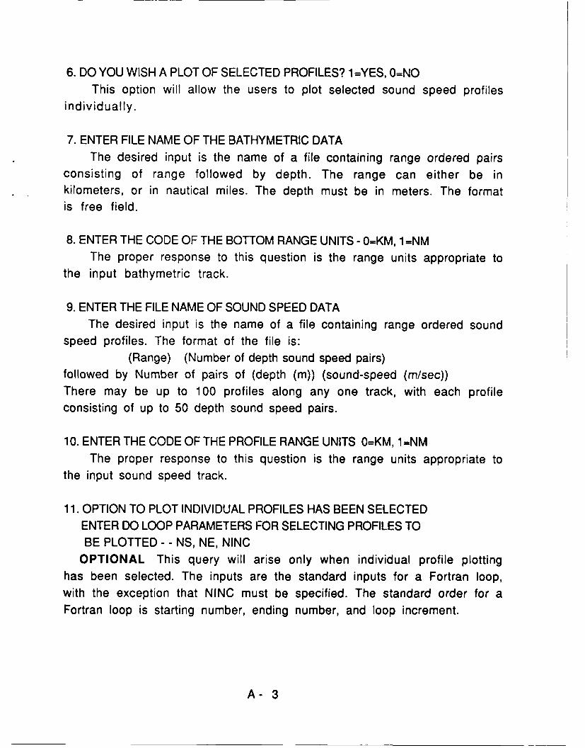
6. DO YOU WISH A PLOT OF SELECTED PROFILES? 1=YES, 0=NOThis option will allow the users to plot selected sound speed profiles

individually.

7. ENTER FILE NAME OF THE BATHYMETRIC DATAThe desired input is the name of a file containing range ordered pairs

consisting of range followed by depth. The range can either be inkilometers, or in nautical miles. The depth must be in meters. The formatis free field.

8. ENTER THE CODE OF THE BOTTOM RANGE UNITS - 0=KM, 1 =NMThe proper response to this question is the range units appropriate to

the input bathymetric track.

9. ENTER THE FILE NAME OF SOUND SPEED DATAThe desired input is the name of a file containing range ordered sound

speed profiles. The format of the file is:(Range) (Number of depth sound speed pairs)

followed by Number of pairs of (depth (m)) (sound-speed (m/sec))There may be up to 100 profiles along any one track, with each profileconsisting of up to 50 depth sound speed pairs.

10. ENTER THE CODE OF THE PROFILE RANGE UNITS O=KM, 1 =NMThe proper response to this question is the range units appropriate to

the input sound speed track.

11. OPTION TO PLOT INDIVIDUAL PROFILES HAS BEEN SELECTEDENTER DO LOOP PARAMETERS FOR SELECTING PROFILES TOBE PLOTTED - - NS, NE, NINC

OPTIONAL This query will arise only when individual profile plottinghas been selected. The inputs are the standard inputs for a Fortran loop,with the exception that NINC must be specified. The standard order for aFortran loop is starting number, ending number, and loop increment.

A- 3

Inputs for Program RAYACTThis section describes the inputs for program RAYACT. RAYACT takes as

input the environmental file generated by program PROFIL, user bottomloss specification, source depths, target depths to produce output datafiles, user specified print files, and the plots specified by the user. Theuser inputs for RAYACT are listed below as they appear when executingthe program.

1. ENTER TITLE FOR RUN (UP TO 68 CHARACTERS)The is an alphanumeric identifier that will appear on the print file and

the ray trace plot (if specified).

2. ENTER THE NAME OF THE OUTPUT PRINT FILEThis is the file name assigned to the output print file generated by the

program, it may be any unique valid name.

3. DO YOU WISH A PRINT FILE OF RAY STATISTICS? N=YES, O=NON=STATUS PRINTED FOR EVERY Nth RAY

Specifying a print file of the ray statistics will give a print fileshowing the statistics (arrival angle, travel time, etc.) for each ray forall boundary interactions, and (if target depths are specified) target depthinteractions.

4. ENTER NAME FOR PRINT FILE FOR RAY STATISTICSOPTIONAL This is the file name assigned to the output ray statistics

print file generated by the program, it may be any unique valid name.

5. ENTER FILE NAME OF INPUT ENVIRONMENT FIELDEnter the file name of the PROFIL output file created using the sound

speed field, and bathymetry that is desired.

A- 4

6. ENTER SOURCE DEPTH (M)Enter the depth in meters of (a) the source if the ray trace originates

from the source location, or (b) the receiver if the ray trace originatesfrom the receiver location.

7. ENTER UP THE 3 TARGET DEPTHS(M): 0 TO STOPEnter the depths of up to three targets in meters. If fewer than three

target depths are specified the the last specified depth must be 0.

8. ENTER RAY TRACING PARAMETERSRINIT(KM), RMAX(KM), NODUC, NBB,

-TMAX(SEC), BLMAX(DB), MAXORDEnter, in order, RINIT the initial range of the ray trace in kilometers

(normally zero), RMAX the final range of the ray trace in kilometers(normally 20 percent beyond the maximum range of interest), NODUC acontrol variable that when set to zero uses the default linearinterpolation between sound speed minimums in adjacent sound speed

profiles, otherwise a location interpolation between adjacent profiles at

the same depth is used (normal value is zero), NBB the number of bottombounces that a ray may take (maximum value is 98), TMAX is the maximumtime a ray is allowed to propagate (if set to zero the maximum rangedetermines the travel time), BLMAX is the maximum bottom loss that a rayis allowed to accumulate before being terminated (the default value is175), and MAXORD is the number of turning points (bottom bounces,

surface bounces, and refractive turning points) that a ray is allowed, themaximum number is 196.

9. DO YOU WISH TO REDEFINE DEFAULT RAY ITERATION PARAMETERS?If you do not wish to redefine the default ray iteration parameters then

enter 0.

10. ENTER ITERATION PARAMETERSDELMIN, DELMAX, HITDEL, VFAEPS, DELSMX

OPTIONAL DELMIN is the minimum range step for a ray, DELMAX is themaximum allowable range step for a ray, HITDEL is the tolerance for

A- 5

boundary or target depth interaction, VFAEPS is the maximum allowableerror in sound speed estimation, and DELSMX is the maximum allowable

change in the sine of the ray.

11. RAY LAUNCH ANGLES ARE SPECIFIED BY FANS(INTERVALS) OF EQUISPACED ANGLES. ANGLESARE MEASURED POSITIVE DOWN AND IN DEGREESENTER NO. OF FANSThe rays that are traced by this version of RAYACT are specified by the

user. They are specified as ray fans, that is fans defined by minimum,incremental, and maximum angles. Inside each ray fan the ray angular

spacing is constant. Approximately 1000 rays can be specified.

12. FAN 'I' ANGST, ANGINC, ANGENDThis entry will be entered the number of times that is specified in the

previous entry. Basically the input is the minimum angle, the incrementalangle, and the maximum angle for each fan. The fans start from -89.6degrees and go to 89.6 degrees with a minimum increment of 0.1 degree.

Do not specify the same angle more than once.

13. ENTER THE SOURCE OF BOTTOM LOSS FOR COMPUTATION1 = BOTTOM LOSS TABLE, 2 = NOO CURVES.

Two choices are given for bottom loss, either a table of values can be

entered into the program via a file, or a NOO province can be specified.

14. ENTER THE NAME OF THE BOTTOM LOSS FILEIf a bottom loss table is specified, then the program will expect a file

name containing the table in the formatnumber of tables (maximum - 4)number of entries in table, maximum range of table

grazing angle, bottom loss (number of entries times)

15. ENTER THE HIGH FREQUENCY BOTTOM LOSS PROVINCEIf the NOO curves are specified, then a single province (1-9) is

specified for the bottom loss.

A- 6

16. DO YOU WISH A PLOT OF RAYPATHS? +N,-N=YES, 0 = NOEVERY Nth RAY PLOTTEDN<0: WILL INPUT MIN, MAX ANGLE (DEF TO -20, +20)

N controls the number of rays plotted. If N is zero then no rays areplotted, N = 1 implies plotting every ray, N = M implies every mth ray willbe plotted.

17. PLOT OF RAY PATHS HAS BEEN REQUESTEDENTER MIN ANGLE, MAX ANGLE, R-AXIS(IN), DP-AXIS(IN)

MAX RANGE(KM), MAX DEPTH(M)The angle entries are in degrees, if n (the control for the number of

lines) is negative the numbers entered will be used. R-AXIS(IN) is thelength of the range axis in inches, DP-AXIS(IN) is the length of the depth

axis in inches. MAX RANGE(KM) is the maximum range to which to plot theray traces, and MAX DEPTH(M) is the maximum depth of the ray trace to beshown on the plot.

18. DO YOU WISH TO SAVE SURFACE ENCOUNTERS? 1-=YES, 0=NOIf you wish to calculate surface reverberation you must save the

surface encounters.

19. ENTER THE NAME FOR STORING SURFACE ENCOUNTERSOPTIONAL Will be queried only if answer to previous question is yes.

This is the file name assigned to the output data file generated by theprogram. This file contains information that is necessary to execute theRTHETA program.

20. DO YOU WISH TO SAVE BOTTOM ENCOUNTERS? 1 =YES, 0=NOIf you wish to calculate bottom reverberation you must save the bottom

encounters.

21. ENTER THE NAME FOR STORING BOTTOM ENCOUNTERSOPTIONAL Will be queried only if answer to previous question is yes.

This is the file name assigned to the output data file generated by the

A- 7

program. This file contains information that is necessary to execute theRTHETA program.

22. DO YOU WISH TO SAVE TARGET DEPTH ENCOUNTER? 1 =YES, O=NOOPTIONAL If a target depth has been specified then you may decide to

save or discard the target depth crossing information

23. ENTER THE NAME FOR STORING DEPTH ENCOUNTERSOPTIONAL Will be queried only if answer to previous question is yes.

This is the file name assigned to the output data file generated by theprogram. This file contains information that is necessary to execute theRTHETA program.

Inputs for Program RTHETAThis section describes the inputs for program RTHETA. RTHETA takes as

input a ray trace file (created by RAYACT) user specified frequency and

beam pattern, and generates a print file, a data file for the programsREVERB, or TLVSR and the plots specified by the user. The user inputs forRTHETA are listed below as they appear when executing the program.

1. TYPE TITLE OF JOB (UP TO 68 CHARACTERS)The is an alphanumeric identifier that will appear on the print file and

the composite environment plot (if specified).

2. ENTER NAME FOR PRINT FILEThis is the file name assigned to the output print file generated by the

program, it may be any unique valid name.

3. ENTER NAME OF INPUT DATA FILE FROM RAYACTThis is a file created by program RAYACT, it can be either a ray trace

file for bottom, surface, or target depth interaction.

4. DO YOU WISH A PLOT OF ORDER CONTOURS? 1-YES, O=NOThis is the option for generating a range versus launch angle plot.

5. ENTER PLOTTING PARAMETERS:

A- 8

RNGAX(IN), RMIN(KM), RSTEP, RMAXANGAX(IN), ANGMN(DGS), ANGSTEP, ANGMX

OPTIONAL If plot is selected then this question appears. RNGAX(IN) is

the length of the range axis in inches, RMIN(KM) is the minimum range toplot, RSTEP is the incremental label range, and RMAX is the maximumrange to plot. ANGAX(IN) is the length of the angle axis in inches,AGMN(DGS) is the minimum angle to appear on the plot, ANGSTEP is theincremental angle for labeling purposes, and ANGMX is the maximum angleto appear on the plot.

6. ENTER KFRQ, KBP, IFOUT, MINO, MAXO, IFANG, IFDELKFRQ is the acoustic frequency in hertz, KBP is the number of elements

in the vertical array (1 is omnidirectional, and 0 means a user suppliedbeam pattern will be read in), IFOUT is the type of data file created, 0implies no data file, 1 implies a ray averaged output file, and 2 implies acaustically corrected output file, MINO is the minimum order to calculate,MAXO is the maximum order to calculate (MINO is 1 for surface or targets,and 2 for bottom, while MAXO has a maximum value of 120), IFANG equals1 implies than a range of angles (not the full fan) is to be processed, andIFDEL equals 1 implies that a launch angle is to be deleted.

7. ENTER NAME FOR OUTPUT DATA FILEFOR INPUT TO TLVSR, OR REVERB

OPTIONAL This is the file name assigned to the output data filegenerated by the program. This file contains information that is necessaryto execute the TLVSR or REVERB programs.

8. ENTER ANGMIN, ANGMAX (DEGS) OF LAUNCH-ANGLES TO PROCESSOPTIONAL Enter the minimum and maximum launch angles to process.

9. ENTER ANGLE (DEGS) TO DELETE

OPTIONAL Enter the launch angle to delete.

A- 9

10. ENTER VERTICAL PHONE SPACING OF ARRAY (WAVELENGTHS), ANDDEGREES OF TILT FROM HORIZONTAL (+ IS DOWN): SP, TILTOPTIONAL Enter the phone spacing is degrees, and the tilt of the array

in degrees. This option assumes that the phones are equispaced, and equi-weighted.

11. ENTER NAME OF INPUT FILE CONTAINING BEAM PATTERNOPTIONAL Enter the name of the file containing the beam pattern you

wish to use. The beam patterns contain 181 values (in dB space) one foreach vertical angle from 90 degrees up to 90 degrees down.

Inputs for Program TLVSRThis section describes the inputs for program TLVSR. TLVSR takes as

input an output file generated by program RTHETA, and produces atransmission loss versus range and optional plots, and vertical arrivalstructure as function of range. The transmission loss files from thesource to target, and receiver to target arm used in ACTENV to produceecho level.

1. ENTER TITLE FOR THIS RUN (UP TO 68 CHARACTERS)The is an alphanumeric identifier that will appear on the print file and

the transmission loss plot (if specified).

2. ENTER IFPRT, IFPLT, IFOUT, IFARRThe symbols IFPRT, IFPLT, IFOUT, IFARR are integer variables that have

the value yes when set to a 1, and no when set to zero. IFPRT asks if aprint file is desired, IFPLT asks if a plot is desirea, IFOUT asks if anoutput file (for use in ACTENV) is desired, and IFARR asks if the verticalarrival structure is to be printed along with the transmission loss.

3. ENTER NAME FOR PRINT FILEThis is the file name assigned to the output print file generated by the

program, it may be any unique valid name.

4. ENTER NAME OF INPUT FILE FROM RTHETA

A- 10

This is the file name of the range versus launch angle data file created

by the program RTHETA.

5. ENTER NAME OF OUTPUT FILEThis is the file name assigned to the output data file generated by the

program. This file contains information that is necessary to calculate atarget echo level using ACTENV.

6. ENTER RGMN(KM), RINC(KM), RGMX(KM)Enter the minimum range, incremental range, and the maximum range

for which the transmission loss is to be calculated. Note the maximumnumber of ranges for which transmission loss ran be calculated is 400.

7. ENTER MAXIMUM NUMBER OF ARRIVALS TO BE FOUNDAT EACH RANGE*** DEFAULT AND MAXIMUM ALLOWABLE = 48.

OPTIONAL IFARR is assigned the value 1. Up to 48 arrivals at each

range can be printed, if you desired less than 48 then enter that number.

8. ENTER PLOTTING PARAMETERS:XAXIS(IN), RGMN(KM), RINC(KM), RGMX(KM)YAXIS(IN), TLMIN(DB), DBINC(+DB), TLMAX(DB), DELY(+DB)

OPTIONAL IFOUT is assigned the value 1. XAXIS(IN) is the length of the

range axis in inches, RGMN(KM) is the minimum range for which

transmission loss is to be plotted (in kilometers), RINC(KM) is the

incremental range for labeling (in kilometers), RGMX(KM) is the maximumrange to be plotted. YAXIS(IN) is the length of the transmission loss axis

in inches, TLMIN(DB) is the minimum transmission loss to be plotted,

DBINC(DB) is the incremental loss value for labeling, TLMAX(DB) is the

maximum transmission loss to be plotted, and DELY(+DB) is the span in dB

of the transmission loss (if TLMIN, TINC, and TLMAX assigned then this

value can be set to zero).

A-11

Inputs for Program REVERBThis section describes the inputs for program REVERB. REVERB takes as

input output files generated by program RTHETA, user specified systemcharacteristics, and scattering strengths. REVERB generates a print fileand a data file for the program ACTENV. The user inputs for REVERB arelisted below as they appear when executing the program.

1. ENTER TITLE FOR THIS RUN (UP TO 68 CHARACTERS)The is an alphanumeric identifier that will appear on the print file and

the composite environment plot (if specified).

2. ENTER FILE NAME FOR PRINT FILEThis is the file name assigned to the output print file generated by the

program, it may be any unique valid name.

3. ENTER KEY FOR TYPE OF CALCULATIONSKEY=1 MONOSTATICKEY=2 QUASI-MONOSTATICKEY=3 BISTATIC

Enter the proper key for the type run being made. If the source andreceiver are identical in type, depth, and location, then monostatic is tobe used. If the source and receiver only vary in depth, or type then quasi-monostatic. If bistatic is specified, then the run must be range

independent.

4. ENTER NVERT, MXHITS, MXHITRNVERT is the number of times that the vertical distribution of

reverberation is to be written (if NVERT is greater than or equal to zero),if negative then the vertical distribution of reverberation is written outat equally spaced times specified by the user. MXHITS is the number ofhits (or total arrivals) in a grid space that are allowed from the source,

and MXHITR is the number from the receiver.

5. ENTER RMINS, RINC, RMAX (KM)

A- 12

Enter the minimum, incremental, and maximum range from the source inkilometers.

6. KEY = 3 (BISTATIC CASE)ENTER RMINR, MRAXR, SEP (KM)

OPTIONAL Enter the minimum and maximum range from the receiver. Ifthe minimum range from the source is zero, then the receiver minimumrange cannot be zero. SEP is the source receiver separation in kilometers.

7. ENTER DURATION OF CW PULSE, SECThe pulse duration in seconds.

8. ENTER INITIAL, TINC, AND FINAL TIMES OF REVERB ENVELOPEThe times for which the envelope is to be calculated, in seconds.

9. ENTER ANGLES FOR VER. DIST. OF REVERB:THETA1, DTHETA, THETA2

OPTIONAL If NVERT is not zero then the vertical reverberation as afunction of time is specified. Enter the minimum, incremental, andmaximum angles for which reverberation is to be calculated. (The limit is181 bins, thus -90, 1, 90 specifies all angles in 1-degree bins).

10. ENTER 'NVERT' TIMES TO FIND VERT REV DISTOPTIONAL If NVERT is positive then you must specify NVERT times for

which vertical distribution of reverberation is to be output.

11. ENTER TIMES TO FINE VERT REV DISTTVERT1, DTVERT, TVERT2

OPTIONAL If NVERT is negative then you specify the initial,incremental, and final times to output vertical distribution ofreverberation (in seconds).

12. ENTER FILE NAME FOR SOURCE CONTOURS FROM RTHETAInput the source output file from RTHETA.

A-13

13. ENTER NUMBER OF BOTTOM BACKSCATTER TYPES TO BE USEDThe limit is four backscattering types.

14. ENTER 'NSCAT' BACKSCATTER TYPES ALONG WITHRANGE OUT TO WHICH KSCAT WILL BE USED.

FOR BOTTOM

KSCAT=FLAG INDICATING TYPE OF BOUNDARY BACKSCATTERINGMODEL WILL BE USED

-1 =UNIT BACKSCATTERING FOR ALL ANGLESO=TABLE OF BACKSCATTERING MODEL TO BE READ IN1 =INTERNAL NRL BACKSCATTERING MODEL-USED2=FREQUENCY-SCALING OF NRL MODEL3=STANDARD MODEL USED

4=URICK ROCK BOTTOM DATA USED5=URICK SAND BOTTOM DATA USED6=URICK SILT BOTTOM DATA USED7=URICK CLAY BOTTOM DATA USED

13. ENTER NUMBER OF SURFACE BACKSCATTER TYPES TO BE USED

14. ENTER 'NSCAT' BACKSCATTER TYPES ALONG WITHRANGE OUT TO WHICH KSCAT WILL BE USED.

FOR SURFACE

KSCAT=FLAG INDICATING TYPE OF BOUNDARY BACKSCATTERINGMODEL WILL BE USED

-1 =UNIT BACKSCATTERING FOR ALL ANGLESO=TABLE OF BACKSCATTERING MODEL TO BE READ IN1 =INTERNAL NRL BACKSCATTERING MODEL-USED2=FREQUENCY-SCALING OF NRL MODEL3=STANDARD MODEL USED

A- 14

15. ENTER BOTTOM BACKSCATTER TYPE, MAX RANGE.For bottom backscattering enter type -1 through 7, along with the

maximum range in kilometers.

16. ENTER SSO, SS, WS, WH FOR STANDARD SCATTERING MODELSOPTIONAL For surface reverberation SSO is the scattering strength at

0 degrees grazing angle, and SS is the sea state, WS is the wind speed, andWH is the save height. Only the sea state, wind speed, or wave height needbe specified.

16. ENTER SS0, SS FOR STANDARD SCATTERING MODELSOPTIONAL For bottom reverberation SSO is the scattering strength at

0 degrees grazing angle, and SS is the scattering strength at 90 degreesgrazing angle.

17. ENTER FILE NAME OF RECEIVER CONTOURS FROM RTHETAOPTIONAL If a quasi-monostatic or bistatic run is specified then the

output from the RTHETA program for the receiver (for the bottom ifbottom reverberation is specified, or surface for surface reverberation).

18. DO YOU WISH TO SAVE RESULTS ON OUTPUT FILEThe responses to this question are 1 = Yes, 0 = No.

19. ENTER NAME FOR OUTPUT FILE OF REVERB ENVELOPE

OPTIONAL This is the file name assigned to the output data filegenerated by the program. This file contains information that is necessaryto execute the ACTENV program when reverberation is required.

20. ENTER FILE NAME FOR OUTPUT OF VERT REVERB DISTOPTIONAL This is the file name assigned to the output data file

generated by the program. This file contains the vertical arrival structurein a binary output format.

A-15

Inputs for Program ACTENVThis section describes the inputs for program ACTENV. ACTENV takes as

input reverberation files generated by the program REVERB for the surface

and bottom, transmission loss files for the source to target, and receiverto target generated by the program TLVSR, and system input parameters.The output is a print file of the bottom and surface reverberationenvelope, and the target echo level, along with a plot of the quantities.The user inputs for ACTENV are listed below as they appear when

executing the program.

1. ENTER TITLE FOR THIS RUNThe is an alphanumeric identifier that will appear on the print file and

the active performance prediction plot.

2. ENTER NAME FOR OUTPUT PRINT FILEThis is the file name assigned to the output print file generated by the

program, it may be any unique valid name.

3. ENTER PING TYPE (1 =CW, 2=PULSE, 3=HFM)CENTER FREQUENCY, PING DURATION:

Enter the type, the center frequency in hertz, and the ping duration in

seconds.

4. ENTER BANDWIDTHEnter the bandwidth of signal in hertz.

5. ENTER TMIN, TMAX, TAVE:Enter the minimum and maximum time for which reverberation is to be

plotted and the averaging window. An averaging window of 0 implies no

averaging.

6. ENTER SOURCE LEVEL PER ELEMENT, NOISE LEVEL,RECEIVER DIRECTIVITY INDEX, NO. ARRAY ELEMENTS

A- 16

Entries are source level per element in dB, the ambient noise level inthe band of interest, the receiver directivity index in dB, and the numberof source elements.

7. ENTER PLOT PARAMETERSENTER TAXIS(IN), TMIN(SEC), TINC(SEC), TMAX(SEC)ENTER YAXIS(IN), YMIN(DB), YINC(DB), YMAX(DB), DELY(DB)

The symbols are.TAXIS length of time axis in inchesTMIN minimum time for which reverberation is plotted in seconds.TINC incremental time for labelsTMAX maximum time for which reverberation is plotted in seconds.YAXIS length of reverberation level axis in inchesYMIN minimum level in dB to be plottedYINC increment level (in dB) for labelsYMAX maximum level in dB to be plotted

DELY difference between minimum and maximum level (can be set tozero if YMIN, YINC, and YMAX are specified)

8. ENTER SPECTRAL SPREADING LOSSFOR SURFACE AND BOTTOM

If an estimate of spreading loss in the observed spectra for surface anbottom reverberation is known it can be entered here, otherwise enterzeroes for both.

9. ENTER SURFACE REVERBERATION ENVELOPESENTER NOREV, IFWGT

NOREV is the number of reverberation envelopes (positive number), andIFWGT is either 0 implying that all envelopes are equally weighted, or 1where envelopes can be weighted by the user.

10. ENTER FILE NAME OF REVERBERATION ENVELOPEEnter a data file (binary file) containing reverberation versus time for

surface interactions from program REVERB.

A-17

11. ENTER WEIGHT FOR THIS ENVELOPEThis question is optional, it is only answered if IFWGT is nonzero.

12. ENTER BOTTOM REVERBERATION ENVELOPESENTER NOREV, IFWGTNOREV is the number of reverberation envelopes (positive number), and

IFWGT is either 0 implying that all envelopes are equally weighted, or 1where envelopes can be weighted by the user.

13. ENTER FILE NAME OF REVERBERATION ENVELOPEEnter a data file (binary file) containing reverberation versus time for

bottom interactions from program REVERB.

14. ENTER WEIGHT FOR THIS ENVELOPEOPTIONAL Answer only if IFWGT is nonzero.

15. IS TARGET ECHO TO BE INCLUDED? 1=YES, O=NOIf a target echo calculation is required, and the transmission losses

from the receiver (and generally source) to the target have been made then

a target echo level can be calculated.

16. ENTER FILE NAME OF TRANSMISSION LOSS FROM THETARGET TO THE RECEIVER

This file is a data file created by TLVSR containing the transmission

loss from the receiver depth to the target depth.

17. IS A DIFFERENT FILE TO BE USED FOR TRANSMISSIONLOSS FROM THE SOURCE TO THE TARGET? 1 =YES, O=NO

If the run was quasi-monostatic, bistatic, or the source had a beam

pattern different from the receiver then the source to target transmission

loss must also be used to obtain a correct target ,c-oo estimate.

18. ENTER FILE NAME OF TRANSMISSION LOSS FROM iE

SOURCE TO THE TARGET

A- 18

This file is a data file created by TLVSR containing the transmissionloss from the source depth to the target depth.

19. ENTER RANGE UNITS OF TL VS R FILES: 1=KM, 2=NMThe range units are normally in kilometers when output by the

transmission loss module (TLVSR) of RASP.

20. ENTER SLE(DB), SEP(KM)

Enter the source level per element for the source and the sourcereceiver separation (in kilometers).

21. ENTER BRG, TASP:BRG =TARGET ASPECT RE RCVR (DGS) - 0 BROADSIDE, +CWTASP=TARGET ASPECT RE BEARING LINE (DGS)

-CW BEARING LINE TO TARGET CENTER LINEEnter the target-receiver geometry as defined.

22. ENTER TS (RE SQ M) VS ASPECT (0BOW, 180=STERN)ENTER NUMBER OF TS VALUES TO FOLLOW

Enter the number of target strength (relative to a square meter) versusgeometric aspect.

23. NOW ENTER 'NTS [AS PECT(DGS), TS(DB)] PAIRS AT ARATE OF ONE PAIR PER LINE

Enter the number of target strengths versus aspect specified in theprevious entry, where the aspect is in degrees, and the target strength is

in dB per square meter.

A-19

APPENDIX B

This appendix gives a list of suggested input values for producingshallow water predictions using this version of the Range DependentActive System Performance model (RASP). These suggestions arespecifically for shallow water, and do not address the more generalquestion of best inputs. The specific recommendations will be givenprogram by program.

TAUNTTAUNT has no user input other than input and output file names.

PROFILPROFIL inputs and output parameters (other than the choice of

entering into the program whether the input units are in kilometers,or nautical miles correctly) are significant for shallow water use.

RAYACTRAYACT has a series of specific input recommendations associated

with the execution of this code. The recommendations are:RMAX(KM) (entry 8) should be set 20 percent more than the

maximum range desired.NODUC (entry 8) should be set to 0NBB (entry 8) should be set to 98TMAX(SEC) (entry 8) should be set at 0BLMAX(dB) (entry 8) should be set to 175MAXORD (entry 8) should be set to 196Entry (9) should be set to 1DELMIN (entry 10) should be set to 5DELMAX (entry 10) should be set to 25 for water less than 100

meters deep, and 50 for water less than 300 meters.No of Fans (entry 11) should be set to 5Entries 11 will then read

-89.5 2.0 -39.5-39.0 0.5 -19.0-18.8 0.2 18.8

B-1

19.0 0.5 39.0

39.5 2.0 89.5

RTHETA

No specific recommendations for shallow water runs using RASP

are made for RTHETA.

TLVSRNo specific recommendations for shallow water runs using RASP

are made for TLVSR.

REVERBUse the default number for MXHITS (maximum number of hits

source), and MXHITR (maximum number of hits receiver) both ofwhich appear in entry 4.

B-2

DISTRIBUTION LIST

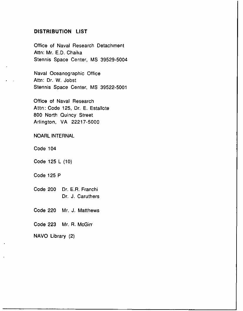
Office of Naval Research DetachmentAttn: Mr. E.D. ChaikaStennis Space Center, MS 39529-5004

Naval Oceanographic OfficeAttn: Dr. W. JobstStennis Space Center, MS 39522-5001

Office of Naval ResearchAttn: Code 125, Dr. E. Estallote800 North Quincy StreetArlington, VA 22217-5000

NOARL INTERNAL

Code 104

Code 125 L (10)

Code 125 P

Code 200 Dr. E.R. FranchiDr. J. Caruthers

Code 220 Mr. J. Matthews

Code 223 Mr. R. McGirr

NAVO Library (2)

REPOT DCUMNTATON AGEForm ApprovedREPOT DCUMNTATON AGEOBM No. 070"-188

Public reporting burden for this collection of information is estimated to average I hour per response, including the time for reviesing instructions, searching existing data sources,gathering and maintaining the data needed, and completing and reviewing the collection of informatic '. Send comments regarding this burden or any other aspet of this collection of information,including suggestions for reducing this burden, to Washington Headquarters Services, Directorate for information Operations and Reports, 1215 Jefferson Davis Highway, Suite 1204, Arlington,VA 22202-4302, and to the Office of Management and Budget, Papenork Reduction Project (0704-0188), Washington, DC 20503.

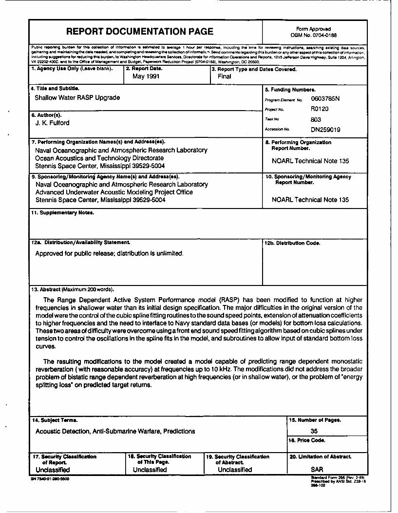
1. Agency Use Only (Leave blank). 2. Report Date. 3. Report Type and Dates Covered.

May 1991 Final

4. Title and Subtitle. 5. Funding Numbers.

Shallow Water RASP Upgrade Progra Elemnt No. 0603785NProect NO. R0120

6. Author(s).J. K. Fulford TkN 803

Acceson No DN259019

7. Performing Organization Names(s) and Address(es). 8. Performing Organization

Naval Oceanographic and Atmospheric Research Laboratory Report Number.

Ocean Acoustics and Technology Directorate NOARL Technical Note 135Stennis Space Center, Mississippi 39529-5004

9. Sponsoring/Monitoring Agency Name(s) and Address(es). 10. Sponsoring/Monitoring AgencyNaval Oceanographic and Atmospheric Research Laboratory Report Number.Advanced Underwater Acoustic Modeling Project OfficeStennis Space Center, Mississippi 39529-5004 NOARL Technical Note 135

11. Supplementary Notes.

12a. Distribution/Avalablity Statement 12b. Distribution Code.

Approved for public release; distribution is unlimited.

13. Abstract (Maximum 200 words).

The Range Dependent Active System Performance model (RASP) has been modified to function at higherfrequencies in shallower water than its initial design specification. The major difficulties in the original version of themodel were the control of the cubic spline fitting routines to the sound speed points, extension of attenuation coefficientsto higher frequencies and the need to interface to Navy standard data bases (or models) for bottom loss calculations.These two areas of difficulty were overcome using a front end sound speed fitting algorithm based on cubic splines undertension to control the oscillations In the spline fits in the model, and subroutines to allow input of standard bottom losscurves.

The resulting modifications to the model created a model capable of predicting range dependent monostaticreverberation (with reasonable accuracy) at frequencies up to 10 kHz. The modifications did not address the broaderproblem of bistatic range dependent reverberation at high frequencies (or in shallow water), or the problem of "energysplitting loss" on predicted target returns.

14. Subject Terms. 1S. Number of Pages.

Acoustic Detection, Anti-Submarine Warfare, Predictions 3516. Price Code.

17. Security Classification 18. Security Classification 19. Security Classification 20. Umitation of Abstractof Report. of This Page. of Abstract

Unclassified Unclassified Unclassified SARS754-1-2810-4M0 Standard Form 298 (Rev. 2-89)

Prscribed by ANSI Sd. Z39-182M-102