sham lu j. quantum mechanics (lecture notes, 2002)(324s)_pqm
TRANSCRIPT
Chapter 1 Contents
1 Fundamentals of Quantum Mechanics 11.1 Introduction . . . . . . . . . . . . . . . . . . . . . . . . . . . . . . . . . . 1
1.1.1 Why should we study quantum mechanics? . . . . . . . . . . . . . 11.1.2 What is quantum theory? . . . . . . . . . . . . . . . . . . . . . . 2
1.2 Pachycephalic Quantum Mechanics . . . . . . . . . . . . . . . . . . . . . 31.2.1 Schrodinger equation for a particle . . . . . . . . . . . . . . . . . 31.2.2 Normalization of the wave function . . . . . . . . . . . . . . . . . 51.2.3 Distinction between the classical wave and the matter wave . . . . 61.2.4 Statistical Interpretation of the Wave Function: Born’s postulate 61.2.5 Particle Flux and Probability Conservation . . . . . . . . . . . . . 7
1.3 The Many Faces of a Quantum State . . . . . . . . . . . . . . . . . . . . 91.3.1 Fourier transforms and Dirac’s delta function . . . . . . . . . . . 91.3.2 Transformation from the position space to the momentum space . 111.3.3 Momentum wave function and probability distribution . . . . . . 121.3.4 The momentum operator . . . . . . . . . . . . . . . . . . . . . . . 131.3.5 State representation in terms of the energy eigenstates . . . . . . 141.3.6 Meaning of the expansion coefficients . . . . . . . . . . . . . . . . 15
1.4 State Vectors . . . . . . . . . . . . . . . . . . . . . . . . . . . . . . . . . 171.4.1 Concept of a state vector . . . . . . . . . . . . . . . . . . . . . . . 171.4.2 Representation of a state vector . . . . . . . . . . . . . . . . . . . 171.4.3 General properties of the state vectors . . . . . . . . . . . . . . . 18
1.5 Observables As Hermitian Operators . . . . . . . . . . . . . . . . . . . . 191.5.1 Definition of a Hermitian conjugate . . . . . . . . . . . . . . . . . 191.5.2 Examples of Hermitian conjugates . . . . . . . . . . . . . . . . . . 201.5.3 Hermitian operator . . . . . . . . . . . . . . . . . . . . . . . . . . 211.5.4 Corollary . . . . . . . . . . . . . . . . . . . . . . . . . . . . . . . 221.5.5 Implication of the corollary . . . . . . . . . . . . . . . . . . . . . 22
1.6 Matrix Representation of a Physical Observable . . . . . . . . . . . . . . 221.6.1 Hermitian matrix . . . . . . . . . . . . . . . . . . . . . . . . . . . 231.6.2 Product of operators . . . . . . . . . . . . . . . . . . . . . . . . . 241.6.3 Expectation value . . . . . . . . . . . . . . . . . . . . . . . . . . . 251.6.4 Examples of a continuous basis set . . . . . . . . . . . . . . . . . 25
1.7 Eigenvalues and Eigenstates of a Physical Observable . . . . . . . . . . . 251.7.1 Definition . . . . . . . . . . . . . . . . . . . . . . . . . . . . . . . 251.7.2 Properties of an eigenstate of an operator A . . . . . . . . . . . . 261.7.3 Theorem . . . . . . . . . . . . . . . . . . . . . . . . . . . . . . . . 26
i
1.7.4 Orthogonality theorem . . . . . . . . . . . . . . . . . . . . . . . . 271.7.5 Gram-Schmidt orthogonalization procedure . . . . . . . . . . . . . 271.7.6 Physical meaning of eigenvalues and eigenstates . . . . . . . . . . 281.7.7 Eigenstate expansion and probability distribution . . . . . . . . . 281.7.8 Important examples of eigenstates . . . . . . . . . . . . . . . . . . 30
1.8 Commutative Observables and Simultaneous Measurements . . . . . . . . 321.8.1 Commutation bracket . . . . . . . . . . . . . . . . . . . . . . . . . 321.8.2 Commutative operators . . . . . . . . . . . . . . . . . . . . . . . . 321.8.3 Theorem 1 . . . . . . . . . . . . . . . . . . . . . . . . . . . . . . . 321.8.4 Example . . . . . . . . . . . . . . . . . . . . . . . . . . . . . . . . 331.8.5 Theorem 2 . . . . . . . . . . . . . . . . . . . . . . . . . . . . . . . 341.8.6 Implications of the theorems . . . . . . . . . . . . . . . . . . . . . 35
1.9 The Uncertainty Principle . . . . . . . . . . . . . . . . . . . . . . . . . . 361.9.1 The Schwartz inequality . . . . . . . . . . . . . . . . . . . . . . . 361.9.2 Proof of the uncertainty principle . . . . . . . . . . . . . . . . . . 371.9.3 Applications of the uncertainty principle . . . . . . . . . . . . . . 38
1.10 Examples . . . . . . . . . . . . . . . . . . . . . . . . . . . . . . . . . . . 411.10.1 The Gaussian wave packet . . . . . . . . . . . . . . . . . . . . . . 411.10.2 Fourier transform of the Yukawa potential . . . . . . . . . . . . . 451.10.3 Interference and beat . . . . . . . . . . . . . . . . . . . . . . . . . 461.10.4 Constant of motion . . . . . . . . . . . . . . . . . . . . . . . . . . 481.10.5 The inversion symmetry . . . . . . . . . . . . . . . . . . . . . . . 491.10.6 The Virial Theorem . . . . . . . . . . . . . . . . . . . . . . . . . . 511.10.7 Translational Symmetry Group . . . . . . . . . . . . . . . . . . . 53
1.11 Problems . . . . . . . . . . . . . . . . . . . . . . . . . . . . . . . . . . . . 58
Chapter 1 List of Figures
1.1 The real part of a Gaussian wave function and its envelope. . . . . . . . 421.2 Probability density from a Gaussian wave function. . . . . . . . . . . . . 421.3 Propagation of a Gaussian wave packet from left to right. . . . . . . . . 43

iv LIST OF FIGURES
Chapter 1
Fundamentals of QuantumMechanics
If a man will begin with certainties, he shall end in doubts;But if he will be content to begin with doubts, he shall end in certainties— Francis Bacon, Advancement of Learning.
1.1 Introduction
1.1.1 Why should we study quantum mechanics?
Quantum mechanics used to be the province of atomic, molecular, nuclear, and particle
physics. In the last four decades, a wide range of development in basic science in astro-
physics, cosmology, quantum optics, condensed matter, chemistry, and materials science
and rapid progress in device technology, such as transistors, lasers, magnetic resonance
imaging, scanning tunneling microscope, optical tweezers and the Hubble telescope, have
made quantum mechanics the fundamental pinning of much of our civilization. Even
the remarkable development of the classical nonlinear dynamics in the 20th century was
rooted in the appreciation of the conceptual and methodology progress in quantum sta-
tistical physics and quantum field theory. The current development of nanoscience in
physics, chemistry, biology and materials science elevates the importance of mesoscopic
physics, a meeting ground of the microscopic and the macroscopic, where not only one
must understanding quantum mechanics but one must also have a clear comprehension
of its influence on the macroscopic outcome. Schrodinger’s cat is no longer merely part
of the gedanken parlor games of the fundamentalists in quantum mechanics. Einstein-
Podolsky-Rosen paradox has evolved into “teleporting”, quantum computing and cryp-
1
2 Chapter 1. Fundamentals of Quantum Mechanics
tography. The availability of lasers and of nanostructures of semiconductors has led to
experimental demonstrations of simple quantum mechanical processes which used to be
subjects of theoretical arguments and only whose consequences in atoms or molecules
are observed. We are no longer content with merely investigating quantum processes
in nature. We now strive to trap atoms, to fabricate designer nanostructures and to
control the outcome of the quantum processes. These are today the many reasons why
an educated person should understand quantum mechanics. It is even more so the case
for a physical scientist or an engineer.
1.1.2 What is quantum theory?
Quantum theory consists in states, observables, and time evolution. In this chapter, we
set up the framework of the quantum theory starting with the familiar wave mechanics
governed by the Schrodinger equation. We shall adopt the axiomatic approach of taking
the Schrodinger equation as given and follow Born in giving the wave function a definite
meaning. Via the various representations of the state in terms of the position, momentum
and energy, we abstract the state as a vector in a space of infinite dimension, independent
of any representation.
In classical mechanics, every dynamical property of a system is a function of the
positions and momenta of the constituent particles and of time. Hence, a dynamical
property is an observable quantity. In quantum theory, we have a prescription to trans-
late a classical property to an operator acting on a wave function. The outcome of a
measurement of a property can only be predicted statistically unless the system is in an
eigenstate of the operator associated with the property. Some pairs of properties, such as
the position and momentum in the same direction, cannot be measured simultaneously
with arbitrarily small uncertainties, thus obeying the uncertainty principle. Other pairs
are not restricted by the uncertainty principle.
In this chapter, we consider the general theory of the physical observables. We wish
to gain a clear picture of what happens after the measurement of a property. It will also
be possible to decide which pair of observables is restricted by the uncertainty principle
and which pair is not.
The time evolution of the state or the observables will be studied in the next chapter.
1.2. Pachycephalic Quantum Mechanics 3
The simplicity of the structure of quantum theory belies the rich texture and the depth
of the theory, the multitude of microscopic phenomena within its grasp, and the subtlety
of the connection to the macroscopic world. The latter are the topics of the rest of the
course.
1.2 Pachycephalic Quantum Mechanics
Pachy — from the Greek word pachys, meaning thick.
Cephalic — pertaining to the head.
Thus, pachycephalosaurus is the name given to a dinosaur with a skull bone nine inches
thick. The moniker “Pachycephalic Quantum Mechanics” imitates the old course popu-
larly known as “Bonehead English”.
You have perhaps seen an attempt to establish wave mechanics in an introductory
course. On the way, you might have gone through a lot of arguments purporting to show
the reasonableness of the extrapolations from classical mechanics. Such an exercise is
valuable in giving physical meaning to the new quantities and equations. For a second
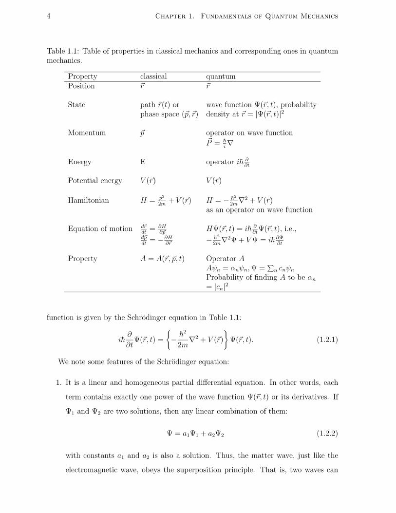
course, we can adopt a simpler route to quantum mechanics. Table 1.1 gives a recipe, with
one column listing the ingredients in classical mechanics and another column transcribing
them to quantum mechanics. One may take the attitude that no amount of arguing about
the reasonableness of the procedure is as conclusive as applying the clear recipe to various
systems and comparing the results to observation. A loftier treatment than the recipe
approach is ‘axiomatic’ quantum mechanics. It sets down axioms or postulates and derive
the Schrodinger equation from them. Such an approach will likely obscure the physical
picture of the wave mechanics. Although we shall not have an exposition of axiomatic
quantum mechanics, it is comforting to know of its existence. You can get a flavor of it
from the book [1] in the bibliography at the end of the chapter.
1.2.1 Schrodinger equation for a particle
For simplicity, consider a point particle with mass m. Extension to a system of many
particles will be done later. Associated with the particle is a wave function Ψ(r, t) from
which we shall deduce the properties of the particle. The time evolution of the wave
4 Chapter 1. Fundamentals of Quantum Mechanics
Table 1.1: Table of properties in classical mechanics and corresponding ones in quantummechanics.
Property classical quantumPosition r r
State path r(t) or wave function Ψ(r, t), probabilityphase space (p, r) density at r = |Ψ(r, t)|2
Momentum p operator on wave functionP = h
i∇
Energy E operator ih ∂∂t
Potential energy V (r) V (r)
Hamiltonian H = p2
2m+ V (r) H = − h2
2m∇2 + V (r)
as an operator on wave function
Equation of motion drdt
= ∂H∂p
HΨ(r, t) = ih ∂∂t
Ψ(r, t), i.e.,dpdt
= −∂H∂r
− h2
2m∇2Ψ + V Ψ = ih∂Ψ
∂t
Property A = A(r, p, t) Operator AAψn = αnψn, Ψ =
∑n cnψn
Probability of finding A to be αn
= |cn|2
function is given by the Schrodinger equation in Table 1.1:
ih∂
∂tΨ(r, t) =
− h2
2m∇2 + V (r)
Ψ(r, t). (1.2.1)
We note some features of the Schrodinger equation:
1. It is a linear and homogeneous partial differential equation. In other words, each
term contains exactly one power of the wave function Ψ(r, t) or its derivatives. If
Ψ1 and Ψ2 are two solutions, then any linear combination of them:
Ψ = a1Ψ1 + a2Ψ2 (1.2.2)
with constants a1 and a2 is also a solution. Thus, the matter wave, just like the
electromagnetic wave, obeys the superposition principle. That is, two waves can
1.2. Pachycephalic Quantum Mechanics 5
be combined to make another wave. The interference and diffraction phenomena
follow immediately.
2. It is a first-order differential equation in time. If the wave function is specified at
any instant for all positions, then it is completely determined at all times.
3. It should satisfy the correspondence principle. In the classical limit (where h is
unimportant), it is possible to find solutions approaching the Newtonian mechanics.
4. The classical wave equation has real coefficients. The complex representation for
the solution is just a convenience. The Schrodinger equation has an imaginary
coefficient and so the solution is in general complex.
1.2.2 Normalization of the wave function
Consider the integral over all space
N =∫
d3r|Ψ(r, t)|2 (1.2.3)
where d3r denotes the volume element dxdydz.
If N = 1, the wave function is said to be normalized. If N is finite, the wave function
is said to be square-integrable. An integrable wave function is trivially normalized by
dividing it with the square root of the integral N .
Some wave functions are not square-integrable, e.g., the plane wave. There are at
least a couple of ways to deal with them. One way is the so-called box normalization.
Take the particle to be in an extremely large box. We are interested in the interior
of the box and the boundary condition and the shape of the box are immaterial. For
example, consider the plane wave in one dimension. Let the wave function be confined
in the interval (−L/2, L/2) where L is enormous compared with the wavelength. Then
the plane wave can be normalized by choosing the constant C to be L−1/2. We shall see
a second way later.
6 Chapter 1. Fundamentals of Quantum Mechanics
1.2.3 Distinction between the classical wave and the matterwave
It might be tempting to conclude that wave mechanics is like the classical theory of waves
and that the particle nature can be completely explained in terms of the latter. It is,
therefore, important to point to a crucial difference between the classical wave and the
quantum wave. The classical wave, say the electromagnetic wave, can be widespread
spatially. It is possible to make a measurement of the wave at a small locality hardly
disturbing the wave elsewhere. Now consider a matter wave representing an electron.
The wave can also be widespread so that there can be diffraction. Is it possible that the
wave represents the structure of the electron spatially? One can trap an electron in a
small locality whereupon there must be no electron wave outside the locality. This is the
crucial difference from the classical wave. It also means that the wave cannot represent
the spatial structure of the electron.
1.2.4 Statistical Interpretation of the Wave Function: Born’spostulate
The classical electromagnetic wave is a measure of the electric or magnetic field. What
property of the material particle does the matter wave represent? We have seen that
a classical interpretation of the wave as the actual structure of the material particle
runs into difficulties. Born suggested that the wave function should be a measure of the
probability of finding the particle at r and t. More precisely,
ρ(r, t) = |Ψ(r, t)|2 (1.2.4)
is the probability density, i.e., the probability of finding the particle in a small volume
d3r at time t is ρ(r, t)d3r. This definition has the following desirable properties:
1. ρ(r, t) is always a real positive number.
2. ρ is large where Ψ is large and small where Ψ is small.
3. If the wave function is normalized (or box normalized),
∫
ρ(r, t)d3r = 1 (1.2.5)
1.2. Pachycephalic Quantum Mechanics 7
meaning that the probability of finding the particle over all space must be unity.
If the wave function is not normalized (or not square-integrable), then ρ(r, t) rep-
resents the relative probability.
Born’s interpretation is statistical. Take the example of a particle in a large box of
volume V under no force otherwise. Let the wave function of the particle be the box-
normalized plane wave (one of an infinite number of possible solutions of the Schrodinger
equation). The probability density is everywhere the same, equal to the constant 1/V .
This gives the chance of locating the particle at one spot. It is as likely to find the particle
at one place as at another. Once the particle is located in a small neighborhood by a
measurement (how small depends on the sensitivity of the measuring instrument), one will
not find it elsewhere immediately afterwards. Thus, the very measuring process changes
the plane wave into a wave function concentrating near that particular neighborhood.
If a large number of measurements are made at a variety of locations, each on one of a
collection of identical boxes, then the position distribution of the particle is given by the
probability density of the wave function.
This represents a radical departure from the Descartes objective reality and the clas-
sical determinism [2]. In quantum theory, there is still determinism in that the wave
function develops according to Schrodinger’s equation. However, we do not know for
sure the properties of a particle at all times but only the probability of the outcome of a
measurement. The very act of observing the particle changes its state. The consequences
of the interaction between the microscopic particle and the macroscopic observer (or the
apparatus) is unavoidable.
1.2.5 Particle Flux and Probability Conservation
As the wave function changes with time, the probability density distribution over space
changes and we can imagine a flow of the probability density has taken place. Since
the probability density function represents the density distribution of a large number of
particles, the flux can represent the particle current density. Denote the flux or current
density by J(r, t). What is the expression of J(r, t) in terms of the wave function?
8 Chapter 1. Fundamentals of Quantum Mechanics
Probability conservation
It follows from the Schrodinger equation that the total probability is time independent.
Consider first the probability in a volume Ω enclosed by a fixed surface S:
P =∫
Ωd3rρ(r, t). (1.2.6)
Now,
∂ρ
∂t= Ψ∗∂Ψ
∂t+
∂Ψ∗
∂tΨ
=1
ih
Ψ∗(
− h2
2m∇2Ψ + V Ψ
)
− Ψ
(
− h2
2m∇2Ψ∗ + V Ψ∗
)
.
By using the Schrodinger equation,
∂ρ
∂t= − h
2miΨ∗∇2Ψ − (∇2Ψ∗)Ψ
= − h
2mi∇ · Ψ∗∇Ψ − (∇Ψ∗)Ψ. (1.2.7)
Let the current density be given by
J(r, t) =h
2miΨ∗∇Ψ − (∇Ψ∗)Ψ. (1.2.8)
The time derivative of the probability in Ω is
dP
dt= −
∫
Ωd3r∇ · J(r, t), using Eq. (1.2.7)
= −∫
SdS · J, (1.2.9)
using the divergence theorem.
For the square-integrable wave function, it tends to zero at infinity and J from Eq.
(1.2.8) does the same. If we let the surface S tend to infinity, then by Eq. (1.2.9)
dP
dt= 0 (1.2.10)
from which the conservation of the total probability over all space follows.
1.3. The Many Faces of a Quantum State 9
Expression for the flux or current density
For a finite volume Ω Eq. (1.2.9) still represents conservation of probability with the
L.H.S. being the rate of increase of the probability balanced by an influx through the
surface S on the R.H.S. Thus, J(r, t) defined by Eq. (1.2.8) is the current density.
Equation (1.2.7) may be rewritten as
∂ρ
∂t+ div J = 0, (1.2.11)
the equation of continuity. For electric charges or fluid, the equation of continuity is a
consequence of the conservation of charges or matter. Equation (1.2.11) is the quantum
mechanical analog.
1.3 The Many Faces of a Quantum State
The wave function Ψ(r, t) which represents the state of a particle is a function of position
and time. It gives us a measure of the probability distribution of the position of the
material particle. Why does the property position enjoys such a privileged position?
Why can’t we replace the position with momentum or energy or any other dynamical
property? In this section, it is shown that indeed the quantum state of a particle can be
represented as a function of momentum or energy.
1.3.1 Fourier transforms and Dirac’s delta function
Definition The Fourier transform ψ(k) of a function ψ(x) is given by
ψ(k) =∫ +∞
−∞
dx√2π
e−ikxψ(x) . (1.3.1)
Fourier theorem If ψ(k) is the Fourier transform of the function ψ(x) as given by
Eq. (1.3.1), then
ψ(x) =∫ +∞
−∞
dk√2π
eikxψ(k) . (1.3.2)
Lemma The Fourier transform of a Gaussian function is another Gaussian.
10 Chapter 1. Fundamentals of Quantum Mechanics
Proof of the lemma is given by putting a Gaussian function
ψ(x) =1√2σ2
e−x2/4σ2
(1.3.3)
with a constant σ into Eq. (1.3.1) and evaluating the integral by completing the square
in the exponent and by using the Gaussian integral,
∫ +∞
−∞dt e−t2 =
√π, (1.3.4)
to obtain the Fourier transform
ψ(k) = e−σ2k2
. (1.3.5)
This lemma can now be used to prove the Fourier theorem and also to introduce
the concept of the Dirac δ-function. Starting from the right-hand side of the theorem,
Eq. (1.3.2), and substituting the definition of the Fourier transform, we obtain
∫ +∞
−∞
dk√2π
eikxψ(k)
=∫ +∞
−∞
dk√2π
eikx∫ +∞
−∞
dy√2π
e−ikyψ(y)
= limσ→0
∫ +∞
−∞
dk√2π
eikx−σ2k2∫ +∞
−∞
dy√2π
e−ikyψ(y)
a harmless introduction of a factor of unity,
= limσ→0
∫ +∞
−∞dy ψ(y)
∫ +∞
−∞
dk
2πeik(x−y)−σ2k2
reversing order of integration,
=∫ +∞
−∞dy ψ(y)δ(x − y)
= ψ(x).
In the last two steps of the proof, we introduced the δ-function
δ(x) = limσ→0
∫ +∞
−∞
dk
2πeikx−σ2k2
, (1.3.6)
1.3. The Many Faces of a Quantum State 11
which by the lemma is
δ(x) = limσ→0
1
2σ√
πe−x2/4σ2
(1.3.7)
= ∞, if x = 0,
= 0, if x = 0. (1.3.8)
The limit yields such a strange function that the mathematicians would say that it is not
a function but a “distribution”. It would be somewhat safer to define the distribution
which the physicists call the δ-function as the limit of a series of well defined functions,
such as in Eq. (1.3.7). See the delightful little book by M.J. Lighthill [3]. It is easy to
verify using the limit definition the two important properties of the δ-function:∫ +∞
−∞dy δ(y) = 1, (1.3.9)
∫ +∞
−∞dy ψ(y)δ(x − y) = ψ(x). (1.3.10)
The limit of Eq. (1.3.6) may be written as
δ(x) =∫ +∞
−∞
dk
2πeikx, (1.3.11)
which is not well defined unless we take it as a shorthand for Eq. (1.3.6) or, alternatively,
as the limit of a finite integral, i.e.
δ(x) = limK→∞
∫ K
−K
dk
2πeikx = lim
K→∞
sin(Kx)
πx. (1.3.12)
1.3.2 Transformation from the position space to the momen-tum space
The Fourier transform of the state wave function Ψ(r) is
Ψ(k) =∫ d3r
(2π)3/2e−ik·rΨ(r). (1.3.13)
By the Fourier theorem,
Ψ(r) =∫ d3k
(2π)3/2eik·rΨ(k). (1.3.14)
This relation may be read as exhibiting the fact that the wave function Ψ(r) is made up
of sinusoidal waves of various wave-vectors k. The Fourier transform Ψ(k) measures the
amount of the sinusoidal wave with wave-vector k in the wave function Ψ(r).
12 Chapter 1. Fundamentals of Quantum Mechanics
1.3.3 Momentum wave function and probability distribution
By the operator form for the momentum given in the Table 1.1, we see that a plane wave
with wave-vector k is an eigenstate of the momentum,
h
i∇ 1
(2πh)3/2eip·r/h = p
1
(2πh)3/2eip·r/h, (1.3.15)
i.e., the plane wave represents a quantum state which carries a definite momentum p = hk.
The constant in front of the plane wave is chosen by normalization.
The Fourier expansion of the wave function, Eq. (1.3.14), may be written in terms of
the momentum eigenvalue p,
Ψ(r) =∫ d3p
(2πh)3/2eip·r/hΦ(p), (1.3.16)
where the coefficient of the expansion,
Φ(p) = Ψ(p/h) ÷ h3/2, (1.3.17)
is the probability amplitude of the momentum by the rules governing the operator in
Table 1.1. The probability density for the momentum value p is
Π(p) = |Φ(p)|2. (1.3.18)
Π(p) is always real and positive and, because we have taken care of the normalization of
the basis states,
∫
d3pΠ(p) =∫
d3p|Φ(p)|2
=∫
d3k|Ψ(k)|2
=∫
d3kΨ∗(k)∫ d3r
(2π)3/2e−ik·rΨ(r)
=∫
d3rΨ∗(r)Ψ(r),
= 1, (1.3.19)
using Eq. (1.3.13) and its complex conjugate.
1.3. The Many Faces of a Quantum State 13
1.3.4 The momentum operator
Sometimes it is too cumbersome to Fourier transform the wave function in order to find
the information about the momentum. In quantum theory, the most information about
the momentum (or position, or any other property) one can have is in its momentum
wave function. A large amount of information is contained in the probability distribution
of the momentum. Equivalent to this latter is the knowledge of all the moments of p. In
practice, one commonly needs or measures only the mean and the variance from repeating
a large number of experiments. It is possible to calculate the mean value of any function of
the momentum directly from the position wave function rather than Fourier transforming
first.
The mean value of the momentum is
〈p〉 =∫
d3p p Π(p)
=∫
d3p Φ∗(p)pΦ(p). (1.3.20)
Differentiating Eq. (1.3.14) with respect to position,
h
i∇Ψ = (2π)−3/2
∫
d3khkeik·rΨ(k). (1.3.21)
Multiplying the equation by Ψ∗ and integrating,
∫
d3rΨ∗ h
i∇Ψ = (2π)−3/2
∫
d3k∫
d3rΨ∗(r)eik·rhkΨ(k)
=∫
d3kΨ∗(k)hkΨ(k)
=∫
d3pΦ∗(p)pΦ(p)
= 〈p〉. (1.3.22)
Similarly, it can be shown that
〈F (p)〉 =∫
d3rΨ∗(r)F
(h
i∇
)
Ψ(r). (1.3.23)
To calculate the mean value of any function of the momentum directly from the position
wave function, one simply replaces the momentum by the momentum operator:
p → P =h
i∇. (1.3.24)
14 Chapter 1. Fundamentals of Quantum Mechanics
We have gone full circle from the momentum operator to the momentum value p and
back.
1.3.5 State representation in terms of the energy eigenstates
Energy eigenstates and eigenvalues
The time development of the wave function of a particle obeys the Schrodinger equation
ih∂
∂tΨ(r, t) = HΨ(r, t), (1.3.25)
where H is the Hamiltonian of the particle. In classical mechanics, the Hamiltonian
is said to be conservative if it does not depend explicitly on time. In that case, the
total energy E is a constant of motion. In quantum mechanics, there is a corresponding
constant energy state.
The energy eigenstate is given by the time-independent Schrodinger equation
Hψ(r) = Eψ(r). (1.3.26)
Or, more explicitly,
− h2
2m∇2 + V (r)
ψ(r) = Eψ(r). (1.3.27)
The time-dependent wave function is given by
Ψ(r, t) = ψ(r)e−iEt/h. (1.3.28)
Orthogonality of eigenstates
Depending on the nature of the potential, the energy eigenvalue can be continuous or
discrete. For the simplicity of exposition, we shall first represent the energy eigenvalues
as discrete. Let us order the energy in increasing values by the integer n. Some of the
energy values may be equal (degenerate).
Hψn(r) = Enψn(r). (1.3.29)
The eigenstates ψn(r) are orthogonal in the sense that for m = n,
〈ψm|ψn〉 ≡∫
d3r ψ∗m(r)ψn(r) = 0, (1.3.30)
1.3. The Many Faces of a Quantum State 15
where we have introduced the angular brackets as the shorthand notation (due to Dirac)
for the integral of the product of the complex conjugate of a wave function with another
wave function. Later, we shall prove that eigenstates of any Hermitian operator (H
being one,) are orthogonal to one another. The eigenfunctions ψn are said to form an
orthonormal set if they are normalized (〈ψn|ψn〉 = 1) and orthogonal to each other, i.e.,
〈ψm|ψn〉 = δmn, (1.3.31)
δmn being the Kronecker delta, zero unless m = n whence it is 1.
Energy eigenstate expansion
If the eigenstates form a complete set, any state of the system with the Hamiltonian H
(or any confined system for that matter) can be expressed as a series
Ψ(r) =∑
n
ψn(r)cn, (1.3.32)
with the constants cn given by
cn = 〈ψn|Ψ〉. (1.3.33)
1.3.6 Meaning of the expansion coefficients
For simplicity, we shall assume here that each energy eigenvalue is nondegenerate. In later
chapters, we shall characterize the degenerate states with additional quantum numbers
such as the angular momentum quantum numbers and include the symmetry considera-
tions of the Hamiltonian. For a general state represented by the wave function (1.3.32),
let us calculate the mean energy,
E = 〈H〉 = 〈Ψ|H|Ψ〉
=∫
d3r Ψ∗(r)H∑
n
ψn(r)cn
=∑
n
En
∫
d3r Ψ∗(r)ψn(r)cn
=∑
n
En|cn|2. (1.3.34)
16 Chapter 1. Fundamentals of Quantum Mechanics
Similarly, the mean value of any function of H, f(H) , is
〈f(H)〉 =∑
n
f(En)|cn|2. (1.3.35)
This is consistent with the last rule in Table 1.1 that the probability of finding the state
Ψ(x) with energy value En is
P (En) = |cn|2. (1.3.36)
Continuous energy eigenvalues
The case of the continuous energy eigenvalues is important in the scattering problem.
The foregoing results are extended by replacing the quantum number n by the continuous
variable E and a set of quantum numbers denoted by λ which distinguishes the states
with the same energy:
Hψλ(r, E) = Eψλ(r, E). (1.3.37)
In the case of a spherically symmetric potential, for example, the quantum numbers
λ stand for the angular momentum quantum numbers , m, which will be derived in
Chapter 4. The orthonormality is replaced by
〈ψλ(E)|ψλ′(E ′)〉 = δ(E − E ′)δλ,λ′ . (1.3.38)
A state can be expressed as an integral of the energy eigenstates:
Ψ(r) =∑
λ
∫
dE ψλ(r, E)cλ(E). (1.3.39)
As an example, the plane wave is an energy eigenstate (as well as a momentum eigenstate)
of a free particle. A state expressed as an integral of the plane waves is related to the
Fourier integral.
Clearly, the foregoing expansion in terms of the eigenstates can be applied to any
Hermitian operator which shares the property of orthonormality. In particular, the prob-
ability meaning of the expansion coefficients holds for any physical property.
1.4. State Vectors 17
1.4 State Vectors
Dirac [4] developed quantum theory in terms of the concept of the state vector and was
able to use it to demonstrate the equivalence between Schrodinger’s wave mechanics and
Heisenberg’s matrix mechanics. We follow the path of the wave function for a state and
make an abstraction of the state as a vector.
1.4.1 Concept of a state vector
A vector in three dimension, v, is an abstract object which represents three numbers
in a Cartesian frame of reference, or an arrow with magnitude and direction in terms
of two angles, etc. By analogy, the state Ψ, which has a representation Ψ(r) in the
position space, Φ(p) in the momentum space, and cλ(E) in the energy space, etc., can be
regarded as a vector in the infinite dimensional vector space (infinite because the number
of eigenstates which serve as a basis set is infinite). To distinguish the state Ψ from its
conjugate Ψ∗, Dirac [4] adopted the notation |Ψ〉 for the former. This is known as the
Dirac “ket” vector. Its Hermitian conjugate, Ψ∗, is represented by the “bra” vector 〈Ψ|as part of the bracket, for, say, the normalization integral 〈Ψ|Ψ〉. If we need to denote
the time dependence, we simply use |Ψ(t)〉.We introduced in the last section the Dirac notation 〈ψm|ψn〉 for the overlap integral
in Eq. (1.3.30) as a matter of convenience. The notation now stands for the inner (or
scalar) product of a bra vector and a ket vector, independent of representation. The
product could equally well have been an integral over wave functions as functions of the
position or momentum variables.
1.4.2 Representation of a state vector
To reverse the process of abstraction of a state vector, we can also choose a complete set
of basis states |q〉, where q denotes a set of quantum numbers such as x, y, z, or px, py, pz,
or E, λ. Then,
|Ψ〉 =∫
dq|q〉〈q|Ψ〉. (1.4.1)
The inner product between the two state vectors, 〈q|Ψ〉, is the probability amplitude of
the state |Ψ〉 being found in state |q〉.
18 Chapter 1. Fundamentals of Quantum Mechanics
To make the vector nature of the state representation more obvious, we introduce a
discrete set of orthonormal states |uj〉, j being chosen as a set of integers. A state vector
is expanded as a series in terms of these basis states:
|ψ〉 =∑
j
|uj〉cj , (1.4.2)
where
cj = 〈uj|ψ〉. (1.4.3)
The explicit matrix form of Eq. (1.4.2) is
|ψ〉 = [|u1〉 |u2〉 . . . ]
c1
c2
.
.
.
(1.4.4)
Instead of using the wave function ψ(r) to represent the dynamical state of a particle at
a particular time, we can use, with respect to the chosen basis set, the column vector
with elements cj, i.e.,
c1
c2
.
.
.
(1.4.5)
1.4.3 General properties of the state vectors
The infinite dimensional vector space of the states |ψ〉 is known as the Hilbert space.
It possesses all the properties of the finite dimensional vector space with which we are
familiar. The overlap integral 〈φ|ψ〉 is the inner (or scalar) product of the two vectors
|φ〉 and |ψ〉. The length of a vector |ψ〉 is defined as√〈ψ|ψ〉. The triangular inequality,
which in the ordinary vector notation is given by
|a +b| ≤ |a| + |b| (1.4.6)
becomes
√
〈ψ + φ|ψ + φ〉 ≤√
〈ψ|ψ〉 +√
〈φ|φ〉. (1.4.7)
1.5. Observables As Hermitian Operators 19
The Schwartz inequality, which for common vectors is given by
|a ·b| ≤ |a| |b| (1.4.8)
becomes
|〈ψ|φ〉|2 ≤ 〈ψ|ψ〉〈φ|φ〉 (1.4.9)
of which we shall have more to say later.
1.5 Observables As Hermitian Operators
Consider a system of one particle only. Extension to many particles will be studied
later. By analogy with the action of the physical observable x or px on the wave function
transforming it to another wave function, each observable property of the system is
represented by an operator A, which acts on a state vector |Ψ〉, transforming it into
another state denoted by |Ψ′〉,
|Ψ′〉 = A|Ψ〉. (1.5.1)
We shall find occasions when it is convenient to use the shorthand AΨ for Ψ′ such that
the transformed state of |Ψ〉 is denoted by |AΨ〉. Examples of observables which we
shall study presently are the position coordinates X, Y, Z, momentum components Px,
Py, Pz, kinetic energy P 2/2m, potential energy V (R ) and the Hamiltonian H. In the
configuration space, the action of the observables x or px on the wave function may be
written as the wave function of the transformed state given by
〈x|X|Ψ〉 = x〈x|Ψ〉, (1.5.2)
〈x|Px|Ψ〉 =h
i
∂
∂x〈x|Ψ〉. (1.5.3)
1.5.1 Definition of a Hermitian conjugate
The Hermitian conjugate of an operator A, denoted by A†, is defined as an operator acting
on the bra state to the left which yields the Hermitian conjugate of the transformed state
resulting from A acting on the ket:
〈Ψ|A† = 〈AΨ|. (1.5.4)
20 Chapter 1. Fundamentals of Quantum Mechanics
As a consequence, the matrix element of the Hermitian conjugate operator with respect
to any two states is given by
〈Ψa|A†|Ψb〉 = 〈AΨa|Ψb〉 = 〈Ψb|AΨa〉∗ = 〈Ψb|A|Ψa〉∗. (1.5.5)
1.5.2 Examples of Hermitian conjugates
1. Position operator: X† = X.
X denotes the position operator for the coordinate x. Thus,
〈Ψa|X†|Ψb〉 = 〈XΨa|Ψb〉 = [〈Ψb|X|Ψa〉]∗
=[∫
d3rΨ∗b(r)xΨa(r)
]∗=
∫
d3rΨ∗a(r)xΨb(r)
= 〈Ψa|X|Ψb〉. (1.5.6)
Since this is true for any two states, the equation X† = X follows. This seems
a rather involved way to show that the coordinate x is real but (1) it does show
the connection between the Hermitian property of an operator and the measurable
number it represents and (2) the logical process involved is a useful exercise in
preparation for a less well-known physical observable.
2. If A is defined as the operator with the position representation ∂∂x
, then A† has the
position representation − ∂∂x
.
To prove this, we start with the right-hand side of the defining equation (1.5.5),
〈AΨa|Ψb〉 =∫
d3r
(∂
∂xΨa
)∗Ψb =
∫
d3r
(∂
∂xΨ∗
a
)
Ψb
=∫
SdSxΨ
∗aΨb −
∫
d3rΨ∗a
∂
∂xΨb, (1.5.7)
having used a variant of the divergence theorem, with S being a large sphere ulti-
mately taken to be infinitely large. If the wave functions vanish at infinity, then the
surface integral tends to zero. Otherwise, the volume integrals are O(V ), where V
is the volume enclosed by S and the surface integral is O(V 2/3), smaller than the
1.5. Observables As Hermitian Operators 21
volume terms. In either case, we have
∫
d3r
(∂
∂xΨa
)∗Ψb =
∫
d3rΨ∗a
(
− ∂
∂x
)
Ψb,
or, 〈AΨa|Ψb〉 = 〈Ψa| − A|Ψb〉 (1.5.8)
Hence, by definition, the Hermitian conjugate of a first-order differential operator
is minus the operator.
3. If a is a complex number and B = aA, then
B† = a∗A†. (1.5.9)
4. If px = −ih ∂∂x
, then
p†x = (−ih)∗(
− ∂
∂x
)
, using Ex. 3 and Ex. 2 above,
= −ih∂
∂x
= px. (1.5.10)
5. The Hermitian conjugate of the Hermitian conjugate of A is A:
(A†)† = A, (1.5.11)
by taking the complex conjugate of the defining equation (1.5.5).
1.5.3 Hermitian operator
The operator A is Hermitian if
A† = A, (1.5.12)
or equivalently, for any two states Ψa and Ψb,
〈Ψa|A|Ψb〉∗ = 〈Ψb|A|Ψa〉. (1.5.13)
Examples of the Hermitian operators are the position operator X, the momentum
Px, and the Hamiltonian H.
22 Chapter 1. Fundamentals of Quantum Mechanics
1.5.4 Corollary
It follows immediately from Eq. (1.5.13) that the mean value of a Hermitian operator for
any state of a system is real.
1.5.5 Implication of the corollary
In classical physics, a physical property usually can take on real values. Although some-
times we use complex properties, they always denote two physical properties. For exam-
ple, the complex electric or magnetic field really represents two properties: the amplitude
and the phase. Or, the complex impedance really represents the resistance and the re-
actance. So let us take a physical property to mean one quantity which, in classical
physics, takes on real values only. We have seen that a physically meaningful quantity is
the mean value of the operator associated with the property with respect to a dynamical
state. By the correspondence principle, it is reasonable to postulate that the mean value
is always real. It follows that an operator which represents a physical observable must
be an Hermitian operator. It is comforting to note that all the operators representing
measurables which we have come across are indeed Hermitian: such as the position, the
momentum, the potential energy, the kinetic energy, the angular momentum and the
Hamiltonian.
1.6 Matrix Representation of a Physical Observ-able
Consider an operator A. It transforms a state |uk〉 to another state A|uk〉, which can be
expanded in terms of the basis set:
A|uk〉 =∑
j
|uj〉Ajk. (1.6.1)
Or in explicit matrix form,
[A|u1〉 A|u2〉 . . .] = [u1〉 |u2〉 . . .]
A11 A12 . . .A21 A22 . . .. . . . . . . . .
. (1.6.2)
Using the orthonormality of the states |uj〉, we have
Ajk = 〈uj|A|uk〉. (1.6.3)
1.6. Matrix Representation of a Physical Observable 23
With respect to the basis set, the operator A can be regarded as a matrix with elements
Ajk. Without fear of confusion, we can use the same symbol A to represent the operator
as well as the matrix.
An operator A acting on a state |ψ〉 changes it into a state |ψ′〉 where
|ψ′〉 = A|ψ〉. (1.6.4)
Let |ψ〉 be represented by a vector c with elements cj given by Eq. (1.4.3) and |ψ′〉 be
represented by the vector c ′ with respect to the same basis set. Then
c′j =∑
k
Ajkck, (1.6.5)
or, in matrix notation,
c ′ = A · c. (1.6.6)
Proof: From Eq. (1.6.1), we have
|ψ′〉 = A|ψ〉 =∑
k
A|uk〉ck =∑
kj
|uj〉Ajkck. (1.6.7)
Multiplying both sides by the bra vector 〈uj|, we obtain Eq. (1.6.5).
The result of an operator A acting on the state |ψ〉 is just a linear transformation of
the state vector c to the state vector Ac.
The inner product of a bra and a ket vector, 〈φ|ψ〉 is a scalar. The outer product of a
ket and a bra is an operator |φ〉〈ψ| transforms any state to the state |φ〉. It is also called
the projection operator. From Eq. (1.6.1), we can express a general operator in terms of
the basis set as
A =∑
j,k
|uj〉Ajk〈uk|. (1.6.8)
1.6.1 Hermitian matrix
From the definition of the Hermitian conjugate, Eq. (1.4.2) the matrix elements of the
conjugate A† are related to those of A by
A†jk = (Akj)
∗, (1.6.9)
24 Chapter 1. Fundamentals of Quantum Mechanics
i.e., to get the matrix A, one not only transposes the matrix A but also takes the complex
conjugate of each element.
For a Hermitian operator A,
Ajk = (Akj)∗, (1.6.10)
or in matrix notation,
A = A†, (1.6.11)
which is of the same form as the operator equation (1.4.9).
1.6.2 Product of operators
The matrix representation of the product AB of two operators A and B is just the matrix
product of the matrices of A and B:
(AB)ij =∑
k
AikBkj. (1.6.12)
Proof: Let C = AB.
C|uj〉 = A(B|uj〉) = A∑
k
|uk〉Bkj
=∑
k
(A|uk〉)Bkj
=∑
ik
|ui〉AikBkj. (1.6.13)
By definition,
C|uj〉 =∑
i
|ui〉Cij. (1.6.14)
By comparing the two sums, we obtain Eq. (1.6.12).
Thus, the operator equation (1.6.13) can also be read as the matrix equation. To find
out whether two operators commute, we simply have to see if the corresponding matrices
commute.
1.7. Eigenvalues and Eigenstates of a Physical Observable 25
1.6.3 Expectation value
〈A〉 = 〈ψ|A|ψ〉 =∑
ij
c∗i Aijcj
= c † · A · c, (1.6.15)
the last expression being in matrix notation, with c as a column vector and c † its Her-
mitian conjugate (a row vector), i.e.
[c∗1 c∗2 . . . ]
A11 A12 . . .A21 A22 . . .. . . . . . . . .
c1
c2
. . .
. (1.6.16)
1.6.4 Examples of a continuous basis set
While it is straightforward to extend the previous results written out in a discrete basis
set to a continuous set, here are some examples where care has to be exercised. For the
position states |x〉,
〈x|X|x′〉 = x〈x|x′〉 = xδ(x − x′), (1.6.17)
〈x|Px|x′〉 =h
i
∂
∂x〈x|x′〉 =
h
i
∂
∂xδ(x − x′), (1.6.18)
using Eqs. (1.5.2) and (1.5.3).
1.7 Eigenvalues and Eigenstates of a Physical Ob-servable
1.7.1 Definition
A state, |ψ〉, which satisfies the equation
A|ψ〉 = α|ψ〉, (1.7.1)
A being an operator and α being a number, is called an eigenstate of the operator A with
the eigenvalue α.
26 Chapter 1. Fundamentals of Quantum Mechanics
1.7.2 Properties of an eigenstate of an operator A
1. Function of an operator
f(A)|ψ〉 = f(α)|ψ〉. (1.7.2)
Starting with Eq. (1.7.1), we can show
A2ψ = A(Aψ) = A(αψ) = α(Aψ) = α2ψ, (1.7.3)
and, by induction, that Eq. (1.7.2) holds for any powers of A. Eq. (1.7.2) is then
valid for any function f(A) which can be expressed as a Taylor series in powers of
A.
2. The mean value of the observable A for the system in an eigenstate is given by the
eigenvalue:
〈A〉 = 〈ψ|A|ψ〉 = α, (1.7.4)
and the uncertainty [defined as the variance, see Eq. (1.7.24)] is zero:
(∆A)2 = 〈A2〉 − 〈A〉2 = α2 − α2 = 0. (1.7.5)
1.7.3 Theorem
Eigenvalues of a Hermitian operator are real.
Proof: Suppose an operator A has an eigenstate |ψ〉 with eigenvalue α.
A|ψ〉 = α|ψ〉. (1.7.6)
Hence,
〈ψ|A|ψ〉 = α〈ψ|ψ〉. (1.7.7)
Since A is Hermitian, taking the complex conjugate of the last equation, we obtain
〈ψ|A|ψ〉∗ = 〈ψ|A†|ψ〉 = 〈ψ|A|ψ〉. (1.7.8)
Therefore,
α∗ = α. (1.7.9)
Q.E.D.
1.7. Eigenvalues and Eigenstates of a Physical Observable 27
1.7.4 Orthogonality theorem
Two eigenstates of a Hermitian operator with unequal eigenvalues are orthogonal.
Proof: Let A be the Hermitian operator and
A|ψi〉 = αi|ψi〉, (1.7.10)
A|ψj〉 = αj|ψj〉, (1.7.11)
where the eigenvalues αi and αj are not equal. Hence,
〈ψj|A|ψi〉 = αi〈ψj|ψi〉, (1.7.12)
and
〈ψi|A|ψj〉 = αj〈ψi|ψj〉. (1.7.13)
Take the complex conjugate of the second equation:
〈ψj|A|ψi〉 = αj〈ψj|ψi〉, (1.7.14)
where on the left we have used the Hermitian property of the operator A and on the
right we have made use of the fact that αj is real and
〈ψi|ψj〉∗ = 〈ψj|ψi〉. (1.7.15)
Subtracting (1.7.14) from (1.7.12),
(αi − αj)〈ψj|ψi〉 = 0. (1.7.16)
Since the two eigenvalues are not equal,
〈ψi|ψj〉 = 0. (1.7.17)
1.7.5 Gram-Schmidt orthogonalization procedure
If the two eigenvalues αi and αj are equal, it is always possible to construct two orthogonal
eigenstates even if |ψi〉 and |ψ〉 are not orthogonal.
|ψ′j〉 = |ψj〉 − |ψi〉
〈ψi|ψj〉〈ψi|ψi〉
, (1.7.18)
is orthogonal to |ψi〉, and is also an eigenstate with the same eigenvalue.
28 Chapter 1. Fundamentals of Quantum Mechanics
1.7.6 Physical meaning of eigenvalues and eigenstates
In quantum mechanics, we represent an observable property by a Hermitian operator.
Because the systems in which we are now interested are microscopic, a measurement of
the property of a system presents a non-negligible interaction of the measuring instrument
with the system under investigation. We postulate that (1) the only possible outcome of
one measurement of the property A is one of the eigenvalues of A, and (2) whatever the
initial state of the system, after the measurement, the system will be in the eigenstate
(or one of the eigenstates, if they are degenerate) whose eigenvalue is the outcome.
If the system is in one of the eigenstates of A before the measurement, a measurement
of the property A will definitely yield the eigenvalue associated with the state, and will
leave the system in the same eigenstate. It follows that the mean value of A is the
eigenvalue and that the uncertainty is zero.
If the system is not in an eigenstate of A, then a measurement of the property A
will put the system in an eigenstate. If the measurement is repeated immediately, the
outcome will be the same eigenvalue and the system stays in the same eigenstate. In
this sense, a measurement is repeatable. The repeated measurement is required to be
performed immediately after the first one because, if the system stays in an eigenstate
of A which is not an eigenstate of the Hamiltonian, given time it will evolve into a state
which is not an eigenstate of A.
1.7.7 Eigenstate expansion and probability distribution
When the system is not in an eigenstate of the Hermitian operator A, it is not possible to
predict exactly which eigenvalue of A will be the outcome of a measurement of A. What
can be done within the framework of quantum mechanics is to examine the mix of the
eigenstates which make up the state of the system and then to give odds on each possible
result, i.e., to associate each eigenvalue of A with a probability of being the outcome of
a measurement.
The orthogonality and completeness theorems enable one to expand any state of the
system in terms of a set of eigenstates of any observable property. Let |ψi〉, i being
a set of integers, be a complete set of orthonormal eigenstates of a Hermitian operator
1.7. Eigenvalues and Eigenstates of a Physical Observable 29
A. (Extension to continuous eigenvalues is straightforward and will be done below by
example. We choose not to burden the notation system to cover the most general case.)
Then
A|ψi〉 = αi|ψi〉, (1.7.19)
〈ψi|ψj〉 = δij. (1.7.20)
Completeness means that any state of the system, represented by the wave function
|Ψ〉 can be expanded as a series in the eigenfunctions:
|Ψ〉 =∑
j
|ψj〉aj. (1.7.21)
To find the coefficients aj, multiply both sides of the equation by 〈ψi|:
〈ψi|Ψ〉 =∑
j
〈ψi|ψj〉aj =∑
j
δijaj
= ai (1.7.22)
The state |Ψ〉 has a probability distribution |aj|2 among the eigenstates |ψi〉 of A.
The reasonableness of the statement is seen as follows. The expectation value of A in
the state |Ψ〉 is, by means of the eigenstate expansion, given by
〈Ψ|A|Ψ〉 =∑
i
αi|ai|2. (1.7.23)
If at a time t, the state of the system is represented by the wave function |Ψ〉, then
|aj|2 is the probability of finding the system to be in the eigenstate ψj immediately after
a measurement of the property A. This probability interpretation is consistent with
the expression for the average value of A given by Eq. (1.7.23) or with the corresponding
expression for any powers of A. The coefficient aj itself is called the probability amplitude.
Besides the expectation value, another important quantity which characterizes the
probability distribution is the uncertainty ∆A, defined by
(∆A)2 = 〈Ψ|A2|Ψ〉 − 〈Ψ|A|Ψ〉2. (1.7.24)
30 Chapter 1. Fundamentals of Quantum Mechanics
1.7.8 Important examples of eigenstates
1. Energy
We have come across this property many times. We take the Hermitian operator
for energy to be the Hamiltonian operator. The eigenfunctions were treated in
Section 1.3.5.
2. Position of a particle
Although we have considered only eigenfunction expansion in the case of discrete
eigenvalues, continuous eigenvalues can be treated in a similar way, for example, by
taking the index to be continuous. The position operator X, when measured, can
yield a continuous spectrum of values x. We express this fact as the eigen-equation:
X|a〉 = a|a〉, (1.7.25)
where |a〉 is the state where the particle is definitely at the coordinate x = a. By
exploiting the property of the δ-function
xδ(x − a) = aδ(x − a), (1.7.26)
we can identify the position eigen-wavefunction for the specific position a as
〈x|a〉 = δ(x − a), (1.7.27)
where x is the position coordinate variable. The equation can also be read as the
orthonormal condition for the position states with continuous eigenvalues. The
position eigenfunction expansion for any state |Ψ〉 is, by extension to continuous
eigenvalues of Eqs. (1.7.21) and (1.7.22),
|Ψ〉 =∫
dx|x〉〈x|Ψ〉, (1.7.28)
where we have used the completeness relation
∫
dx |x〉〈x| = 1. (1.7.29)
The probability 〈x|Ψ〉 is the wave function Ψ(x).
1.7. Eigenvalues and Eigenstates of a Physical Observable 31
3. Momentum of a particle
The momentum operator P in a particular direction (say, along the x axis) is
another example of a property which has continuous eigenvalues p:
P |p〉 = p|p〉. (1.7.30)
Capping both sides of Eq. (1.7.30) leads by means of Eq. (1.5.3) to
h
i
∂
∂x〈x|p〉 = p〈x|p〉. (1.7.31)
Integration of the above leads to the momentum eigen-wavefunction
〈x|p〉 = Ceipx/h, (1.7.32)
with the normalization constant C to be determined.
The orthonormality condition of the momentum eigenstates
〈p|p′〉 =∫
dx|C|2e−ipx/heip′x/h = δ(p − p′) (1.7.33)
leads to
|C|22πh = 1, (1.7.34)
or
C =1√2πh
, (1.7.35)
with the arbitrary choice of zero phase for C.
A general state of the particle has the momentum eigenfunction expansion
|Ψ〉 =∫
dp|p〉〈p|Ψ〉, (1.7.36)
which in the position representation is the Fourier relation:
〈x|Ψ〉 =∫
dp〈x|p〉〈p|Ψ〉 (1.7.37)
where the momentum probability amplitude Φ(p, t) = 〈p|Ψ(t)〉 is just the Fourier
transform of the wave function.
32 Chapter 1. Fundamentals of Quantum Mechanics
1.8 Commutative Observables and Simultaneous Mea-surements
According to Heisenberg’s uncertainty principle, a conjugate pair of dynamic variables
in the classical mechanics sense, such as x and px, cannot be measured simultaneously
to arbitrary accuracy in the quantum regime. A more convenient criterion to determine
if a pair of physical observables can be measured simultaneously is the commutability of
their corresponding operators.
1.8.1 Commutation bracket
Let A and B be two operators representing two observables. Their commutation bracket
is defined by:
[A, B] = AB − BA. (1.8.1)
1.8.2 Commutative operators
Two operators A and B are said to be commutative if
AB = BA, or [A, B] = 0. (1.8.2)
1.8.3 Theorem 1
If A and B are two commutative operators and either A or B has non-degenerate eigen-
values, then its eigenfunctions are also eigenfunctions of the other operator.
Proof: Say, A|ψj〉 = αj|ψj〉, (1.8.3)
with |ψj〉 being non-degenerate, i.e., all the eigenvalues αj are distinct.
Operating on both sides of (1.8.3) with B:
BA|ψj〉 = B(αj|ψj〉) = αjB|ψj〉. (1.8.4)
Since it is given that
AB = BA, (1.8.5)
1.8. Commutative Observables and Simultaneous Measurements 33
Eq. (1.8.4) becomes
A(B|ψj〉) = αj(B|ψj〉), (1.8.6)
which means that B|ψj〉 is also an eigenfunction of A with the eigenvalue αj. Since
we assume that the eigenvalue αj only has one eigenfunction, B|ψj〉 and |ψj〉 must be
essentially the same function, i.e.
B|ψj〉 = βj|ψj〉, (1.8.7)
for some constant βj. But, that means |ψj〉 is an eigenfunction of B with the eigenvalue
βj. QED.
1.8.4 Example
Consider a free particle in one dimension. The momentum operator p and the Hamilto-
nian H, where
H =p2
2m, (1.8.8)
are clearly two operators which commute, i.e.,
[p, H] = 0. (1.8.9)
The plane wave eikx which has a constant wave vector k is an eigenfunction of the
momentum operator p with the eigenvalue hk. It is non-degenerate. Therefore, by the
foregoing theorem, the plane wave eikx must be an eigenstate of the Hamiltonian H,
which can be checked explicitly:
Heikx =
(h2k2
2m
)
eikx. (1.8.10)
We note the non-degeneracy requirement of the theorem. The eigenstates of the
Hamiltonian are doubly degenerate and they are not necessarily the eigenstates of the
momentum even though the two properties commute. From Eq. (1.8.10), it can be seen
that eikx and e−ikx are two degenerate eigenstates of the Hamiltonian with the same
energy value h2k2/2m. These states happen to be also eigenstates of the momentum.
34 Chapter 1. Fundamentals of Quantum Mechanics
However, we could have chosen two different linear combinations as the two degenerate
eigenstates for the same energy eigenvalue, such as the even and odd parity solutions
ψs =1
2(eikx + e−ikx) = cos kx, (1.8.11)
ψa =1
2i(eikx − e−ikx) = sin kx, (1.8.12)
which clearly are energy eigenstates with the same eigenvalue h2k2/2m. Indeed, they are
not eigenstates of the momentum, since
pψs = −ih∂
∂xcos kx = ihk sin kx = ihkψa, (1.8.13)
and
pψa = −ihkψs. (1.8.14)
From these two linear equations, it is easy to construct the eigenstates of p. By
inspection, they are ψs ± iψa.
1.8.5 Theorem 2
If A and B are two commutative operators, then there exists a complete set of eigenstates
which are simultaneously eigenstates of A and B.
Proof: Let us forget the proof of the completeness and concentrate on the existence of a
set of common eigenstates.
Case I. If the eigenstates of one of the operators are all non-degenerate, then Theorem
1 gives the result.
Case II. Some of the eigenstates, say of A, are degenerate. Let us illustrate the proof
with just two-fold degeneracy:
A|ψj〉 = α|ψj〉, for j = 1, 2. (1.8.15)
The proof can be extended straightforwardly to any multiple fold of degeneracy.
By using the comutativity of A and B, we can show that B|ψj〉 is also an eigenstate
of A with the same eigenvalue α:
A(B|ψj〉) = BA|ψj〉 = αB|ψj〉. (1.8.16)
1.8. Commutative Observables and Simultaneous Measurements 35
Since we assume that there are only two eigenstates with the eigenvalue α, the two
states B|ψ1〉 and B|ψ2〉 must be linear combinations of the eigenstates |ψ1〉 and |ψ2〉:[
B|ψ1〉 B|ψ2〉]
=[|ψ1〉 |ψ2〉
] [b11 b12
b21 b22
]
, (1.8.17)
where the bij’s are constants. If the off-diagonal elements b12 and b21 are not both zero,
then |ψ1〉 and |ψ2〉 are not eigenstates of B.
However, it is possible to choose two linear combinations of the eigenstates of A, |ψ1〉and |ψ2〉, which, of course, are still eigenstates of A with the same eigenvalue α, and
which are now eigenstates of B as well, i.e.,
B(|ψ1〉c1 + |ψ2〉c2) = β(|ψ1〉c1 + |ψ2〉c2), (1.8.18)
where B is an operator acting the state wave functions |ψ1〉, and |ψ2〉, β is an eigenvalue of
B, and c1 and c2 are scalar coefficients. Substituting Eq. (1.8.17) into the above equation
and identifying the coefficients of |ψ1〉 and |ψ2〉, we arrive at the secular equation:[
b11 b12
b21 b22
] [c1
c2
]
= β
[c1
c2
]
. (1.8.19)
By diagonalizing the 2 × 2 matrix with coefficients bij, we find two eigenvalues βi,
with i = 1, 2, and their corresponding eigenvectors
[c1i
c2i
]
.
1.8.6 Implications of the theorems
These theorems enable us to decide whether it is possible to measure two observables
simultaneously to any desired accuracy or whether the observables obey the uncertainty
principle.
If the two observables A and B commute, then it is possible to find or prepare the
system to be in a state which is the common eigenstate of both operators, in which the
measured values for A and B can both be accurate to any arbitrary degree. Examples of
such pairs of properties are components of position in two different directions, components
of momentum in two different directions, and energy and momentum for a free particle.
Generalization of the position eigenstate |x〉 to three dimensions is now trivial. Since
the three components X, Y, Z of the position vector operator R commute with each
other, we can have a simultaneous eigenstates of all three position coordinates |r〉 with
36 Chapter 1. Fundamentals of Quantum Mechanics
eigenvalues r = (x, y, z). Similarly for the momentum eigenstate |p〉 in three dimension.
The transformation matrix between the two spaces is
〈r|p〉 =1
(2πh)3/2eip·r/h (1.8.20)
For a pair of observables which do not commute, we give the following generalized
statement of the uncertainty principle.
1.9 The Uncertainty Principle
Denote the commutation bracket of a pair of physical observables, represented by the
Hermitian operators A and B by
[A, B] = iC, (1.9.1)
then C must be either a real constant or a Hermitian operator. A and B are said to be
conjugate observables. For any state of the system,
∆A · ∆B ≥ 1
2|〈C〉|. (1.9.2)
1.9.1 The Schwartz inequality
We need this lemma to prove the general uncertainty principle. For any two states Φ
and Ξ,
|〈Ξ|Φ〉|2 ≤ 〈Ξ|Ξ〉 · 〈Φ|Φ〉 (1.9.3)
This inequality is the functional analog of the vector inequality
|a ·b|2 ≤ |a|2|b|2. (1.9.4)
We give a proof which relies on the geometrical meaning of the vector inequality. The
projection b · a/|b| is the magnitude of the component of vector a along the direction of
b. The magnitude of the component of a perpendicular to b is |a −b(b · a/)|b|2| which
cannot be less than zero. Squaring and expanding this expression will lead to the vector
inequality. So we follow the same method for the two states:[
〈Ξ| − 〈Ξ|Φ〉〈Φ|Φ〉〈Φ|
] [
‖Ξ〉 − |Φ〉 〈Φ|Ξ〉〈Φ|Φ〉
]
≥ 0. (1.9.5)
Expansion of this inequality leads to the Schwartz inequality.
1.9. The Uncertainty Principle 37
1.9.2 Proof of the uncertainty principle
Suppose the system is in the state |Ψ〉. It is convenient to change the operator to one
with zero expectation value in that state, e.g.,
δA = A − 〈A〉, (1.9.6)
〈A〉 being the shorthand for the mean value 〈Ψ|A|Ψ〉.To facilitate the use of the Schwartz inequality, we let
|Ξ〉 = δA|Ψ〉,
|Φ〉 = δB|Ψ〉. (1.9.7)
Since δA and δB are Hermitian operators, it is easy to show that the uncertainties are
given by
(∆A)2 = 〈Ξ|Ξ〉
(∆B)2 = 〈Φ|Φ〉. (1.9.8)
The Schwartz inequality (1.9.3) then takes us a step towards the uncertainty relation:
(∆A)2(∆B)2 ≥ |〈Ξ|Φ〉|2, (1.9.9)
where,
〈Ξ|Φ〉 = 〈Ψ|δA δB|Ψ〉, (1.9.10)
having used the Hermitian property of A. The product operator may be written in terms
of the symmetrized and antisymmetrized products:
δA δB = S + iT, (1.9.11)
where S =1
2(δA δB + δB δA) ≡ 1
2δA, δB, (1.9.12)
T =1
2i(δA δB − δB δA) ≡ 1
2i[δA, δB], (1.9.13)
38 Chapter 1. Fundamentals of Quantum Mechanics
so that both the expectation values 〈S〉 and 〈T 〉 are real. We have introduced the
anticommutation brackets A, B = AB + BA in addition to the commutation brackets.
The expectation value of T is
〈T 〉 =1
2i〈[A, B]〉 =
1
2〈C〉. (1.9.14)
Hence,
|〈Ξ|Φ〉|2 = |〈S + iT 〉|2
= |〈S〉|2 + |〈T 〉|2
≥ |〈T 〉|2 =1
4|〈C〉|2. (1.9.15)
The symmetrized part 〈S〉 is a measure of the correlation between the two operators δA
and δB, which is an important quantity in quantum dynamics. It also contributes to
the product of the uncertainties. Since the correlation may exist also in the classical
regime, this portion of the uncertainty is not necessarily quantum in nature. The anti-
symmetrized part which provides the minimum uncertainty product is quintessentially
quantum mechanical since all classical observables commute.
From the general statement of the uncertainty principle here we can derive the special
case for the pair of operators x and px. Since [x, px] = ih, then
∆x∆px ≥ 1
2h. (1.9.16)
1.9.3 Applications of the uncertainty principle
We have seen that the uncertainty principle is a consequence of the quantum mechanics.
It is a succinct statement of an essentially quantum phenomenon. It is also useful in two
aspects: it provides a physical understanding of some microscopic phenomena completely
outside the realm of classical physics and it can be used to yield some semi-quantitative
estimates.
A particle under gravity
Consider a familiar problem in mechanics. A particle falls under gravity towards an
impenetrable floor. According to classical mechanics, the ground state (the state of least
1.9. The Uncertainty Principle 39
energy) is one in which the particle is at rest on the floor. Let us measure the distance
vertically from the floor and call it x. Thus, we know the position of the particle in its
ground state (x = 0) and also its momentum (p = 0). This contradicts the uncertainty
principle.
We can solve the problem by quantum mechanics. The potential energy of the particle
is
V (x) = mgx if x > 0,= +∞ if x < 0.
(1.9.17)
Just plug this into the Schrodinger equation and solve it. Let us try a simple estimate
here. The ground state will differ from the classical solution by having an uncertainty in
position of ∆x and momentum ∆p where
∆p ∼ h/∆x. (1.9.18)
Then the energy is approximately,
E ∼ (∆p)2
2m+ mg∆x ∼ h2
2m(∆x)2+ mg∆x. (1.9.19)
Minimizing the energy with respect to ∆x, we obtain
∆x ∼(
h2
m2g
)1/3
∼(
me
m
)2/3
× 1.11 × 10−3meter. (1.9.20)
where me is the mass of the electron.
From the uncertainty principle, we have deduced that a particle cannot rest on a floor
even under the pull of gravity. Even in the lowest energy state, the particle bounces up
and down with a range given by (1.9.20).
Stability of the electron orbit in an atom
Bohr had postulated that the orbits are ‘stationary.’ Once we accept the uncertainty
principle, we can understand the stability of the smallest Bohr orbit. Consider the
hydrogen atom. We shall come back to the detailed solution of the Schrodinger equation
later. The electron is prevented from radiating electromagnetic energy and falling into
the nucleus by the following considerations. The closer the electron gets to the nucleus,
the larger the uncertainty of its momentum is. Then there is the possibility that its
40 Chapter 1. Fundamentals of Quantum Mechanics
kinetic energy becomes larger than its potential energy, thus escaping from the nucleus.
Therefore, in the ground state, the electron compromises by staying at a distance from
the nucleus.
We can obtain a more quantitative estimate. Let the root-mean-square distance of
the electron from the proton be ∆r. The uncertainty in momentum is
∆p ∼ h/∆r. (1.9.21)
The energy of the ground state is roughly,
E ∼ (∆p)2
2m− e′2
∆r
∼ h2
2m(∆r)2− e2
∆r. (1.9.22)
where, in SI units, e′2 = e2/4πε0, e being the proton charge. The minimum energy is
given by
∆r ∼ h2/me2 = a0 ∼ 0.5 A, (the Bohr radius). (1.9.23)
It is a fluke that we obtain exactly the right energy because in (1.9.18) we can only be
certain to an order of magnitude of the coefficient multiplying h.
From Eq. (1.9.20), the range of bounce of a ground state electron on the floor under
gravity is about 1 mm, surprisingly large compared with the uncertainty in position in
the atom. The reason is that the force of attraction on the electron by the proton is much
stronger than the gravity pull. Another inference is that the stronger the attraction, the
larger the range of possible speed. For the hydrogen atom, the speed is about 106 m/s
which is small enough compared with the speed of light that non-relativistic mechanics
is valid. For inner electrons in very heavy atoms or nucleons (neutrons and protons) in
the nucleus, the force of attraction is much stronger and the speed of the particle is close
enough to c that relativistic quantum mechanics must be used.
Time for the spread of a wave-packet
In section 1.10.1, an explicit calculation yields the time taken to double the width of a
Gaussian wave-packet. Here is a more general derivation for the order of magnitude of
the time T .
1.10. Examples 41
Suppose a wave-packet initially has uncertainty ∆x in position and ∆p in momentum.
Initially, the wave-packet has components of plane waves with wave-vectors in a range
∆p/h. Consider the motion of two components of plane waves, one with the wave-vector
of the mean and one with wave-vector differing by one standard deviation. The two plane
waves have wave-vectors different by ∆p/h and, therefore, speeds differing by ∆p/m. If
initially the two plane waves both have crests at the average position of the wave-packet,
after time T , they will be at a distance T∆p/m apart. Since T is the time taken for the
wave-packet to double its width, this distance T∆p/m must be of the same order as the
initial width ∆x:
∆x ∼ T∆p/m. (1.9.24)
Hence,
T ∼ m∆x/∆p ∼ m(∆x)2/h. (1.9.25)
in agreement with Eq. (1.10.9).
1.10 Examples
Example is the school of mankind, and they will learn at no other. – Edmund Burke
1.10.1 The Gaussian wave packet
Given that at t = 0 the particle is at x = 0±σ (with uncertainty σ in position) and with
mean momentum hK, what happens to the particle at a later time t?
The information which we possess is not sufficient to determine the wave function at
t = 0 completely. A reasonable approximation for the initial wave function which agrees
with the given data is
Ψ(x, 0) = f(x) = (2πσ2)−1/4 exp
(
− x2
4σ2+ iKx
)
, (1.10.1)
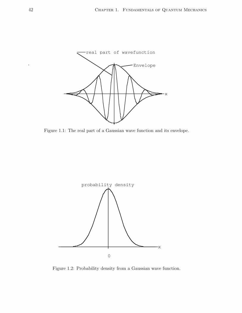
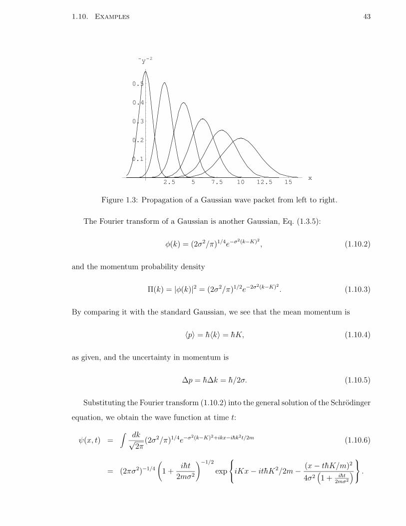
with the mean position at x = 0 and the uncertainty ∆x = σ. The initial wave function
is modulated with a Gaussian envelope (Fig. 1.1) and the probability density is Gaussian
(Fig. 1.2).
x
real part of wavefunction
Envelope
x
probability density
0
42 Chapter 1. Fundamentals of Quantum Mechanics
Figure 1.1: The real part of a Gaussian wave function and its envelope.
Figure 1.2: Probability density from a Gaussian wave function.
1.10. Examples 43
2.5 5 7.5 10 12.5 15x
0.1
0.2
0.3
0.4
0.5
¨y¨2
Figure 1.3: Propagation of a Gaussian wave packet from left to right.
The Fourier transform of a Gaussian is another Gaussian, Eq. (1.3.5):
φ(k) = (2σ2/π)1/4e−σ2(k−K)2 , (1.10.2)
and the momentum probability density
Π(k) = |φ(k)|2 = (2σ2/π)1/2e−2σ2(k−K)2 . (1.10.3)
By comparing it with the standard Gaussian, we see that the mean momentum is
〈p〉 = h〈k〉 = hK, (1.10.4)
as given, and the uncertainty in momentum is
∆p = h∆k = h/2σ. (1.10.5)
Substituting the Fourier transform (1.10.2) into the general solution of the Schrodinger
equation, we obtain the wave function at time t:
ψ(x, t) =∫ dk√
2π(2σ2/π)1/4e−σ2(k−K)2+ikx−ihk2t/2m (1.10.6)
= (2πσ2)−1/4
(
1 +iht
2mσ2
)−1/2
exp
iKx − ithK2/2m − (x − thK/m)2
4σ2(1 + iht
2mσ2
)
.
44 Chapter 1. Fundamentals of Quantum Mechanics
The wave function is a plane wave with a Gaussian envelope. At time t, the mean position
is
〈x〉 = hKt/m, (1.10.7)
with uncertainty
∆x = σ
1 +
(ht
2mσ2
)2
1/4
. (1.10.8)
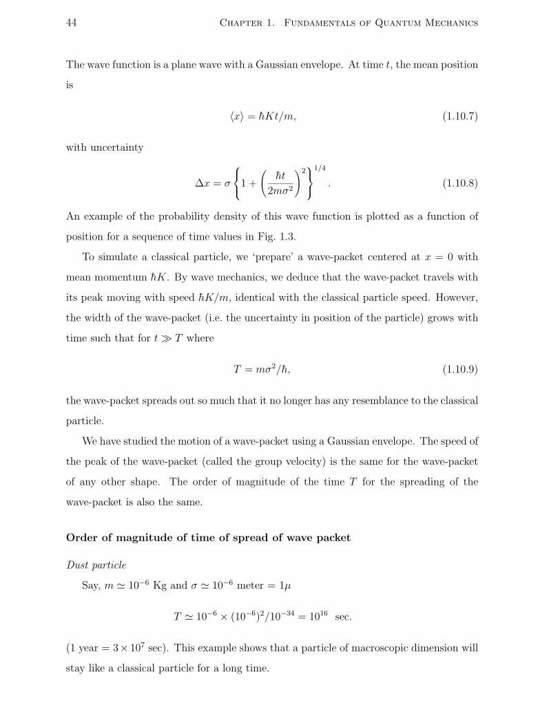
An example of the probability density of this wave function is plotted as a function of
position for a sequence of time values in Fig. 1.3.
To simulate a classical particle, we ‘prepare’ a wave-packet centered at x = 0 with
mean momentum hK. By wave mechanics, we deduce that the wave-packet travels with
its peak moving with speed hK/m, identical with the classical particle speed. However,
the width of the wave-packet (i.e. the uncertainty in position of the particle) grows with
time such that for t T where
T = mσ2/h, (1.10.9)
the wave-packet spreads out so much that it no longer has any resemblance to the classical
particle.
We have studied the motion of a wave-packet using a Gaussian envelope. The speed of
the peak of the wave-packet (called the group velocity) is the same for the wave-packet
of any other shape. The order of magnitude of the time T for the spreading of the
wave-packet is also the same.
Order of magnitude of time of spread of wave packet
Dust particle
Say, m 10−6 Kg and σ 10−6 meter = 1µ
T 10−6 × (10−6)2/10−34 = 1016 sec.
(1 year = 3×10⁷ sec). This example shows that a particle of macroscopic dimension will
stay like a classical particle for a long time.
1.10. Examples 45
Electron
m 10−30 kg
T 104 × σ2 sec.
(i) Electron in an atom
σ size of atom a0 = 0.5 × 10⁻¹⁰ meter.
T 10−16 sec.
From the Bohr theory of the hydrogen, in particular Eqs. (1.6.5) and (1.6.6), for the
electron in its ground state the period of revolution around the proton is about 10−16
sec. Hence, it is impossible to make a wave-packet for the electron in an atom and to try
to follow its progress.
(ii) Electron in a thermionic tube
Energy E 5 ev 10−18J.
Speed v (2E/m)1/2 106 m/s.
The time taken by the electron to travel 1 cm is about 10−8 sec, 1 centimeter being taken
as the order of magnitude dimension of the thermionic tube. If the electrons can be
treated as classical particles, then T >∼
10−8 sec and σ = (10−4T )1/2 >∼
10−6 meters. The
uncertainty in position is a lot larger than the atomic dimension.
1.10.2 Fourier transform of the Yukawa potential
Here is an example of Fourier transform in three dimensions. Find the Fourier transform
of the potential
V (r) =e−αr
r, (1.10.10)
where r is the radial distance from the origin.
Solution — The Fourier transform of the potential is given by
U(k) =∫
d3r1
re−αr−ik·r, (1.10.11)
46 Chapter 1. Fundamentals of Quantum Mechanics
where we find it convenient to drop the factor (2π)−3/2 in the Fourier integral here and
put it in the inverse Fourier integral. In the spherical polar coordinates (r, θ, φ) with the
z-axis chosen along the wave vector k, the integral is
U(k) =∫ ∞
0r2dr
∫ π
0sin θdθ
∫ 2π
0dφ
1
re−αr−ikr cos θ
= 2π∫ ∞
0rdr
∫ 1
−1dµ e−αr−ikrµ
= 4π∫ ∞
0dr
[1
ke−αr+ikr
]
=4π
α2 + k2, (1.10.12)
where [ ] denotes the imaginary part of the expression in the square brackets and we
have changed the variable µ = cos θ for the θ integration.
As a bonus, by taking the limit of α to zero, we find the Fourier transform of the
Coulomb potential 1/r to be 4π/k2.
1.10.3 Interference and beat
1. The wave function of a free particle in one dimension at time t = 0 is made up of
two plane waves of the same amplitude with wave-vectors k1 and k2:
ψ(x, t = 0) = C(eik1x + eik2x) . (1.10.13)
Find the wave function at time t. What is the probability of finding the particle at
time t with momentum hk1?
Solution — The most general way to find the solution at time t is by Fourier
transforming the solution at t = 0. Since Fourier transform is just a way to decom-
pose a function of x into plane-wave components and since we are already given a
discrete sum of two plane waves which is a special case of the Fourier integral, we
can simply proceed to find the time dependence of each plane wave which satisfies
the Schrodinger equation and place them back into the sum which will then be a
solution of the Schrodinger equation, i.e.
ψ(x, t) = C(eik1x−iω1t + eik2x−iω2t) , (1.10.14)
1.10. Examples 47
where
ωn =hk2
n
2m. (1.10.15)
The moduli squared of the coefficients in front of the plane waves give the relative
probabilities of finding the particle in the respective plane-wave states. Thus, the
probability of finding it in k1 state is one-half.
2. Suppose k1 = k and k2 = −k. Find the wave function at time t and discuss the
interference effect by contrasting the probability density of the wave function with
that of each plane-wave component alone.
Solution — The wave function is
ψ(x, t) = 2C cos(kx)e−iωt, (1.10.16)
with
ω =hk2
2m. (1.10.17)
The probability density distribution is
ρ(x, t) = |ψ(x, t)|2 = 4|C|2(cos kx)2, (1.10.18)
which varies sinusoidally between 0 and 4|C|2, in contrast with the constant density
associated with a single plane wave.
3. Suppose k1 = k − ∆k and k2 = k + ∆k, ∆k k. Describe the resultant wave
function. Find the speed of the “beat” pattern. Show that the current density
satisfies the equation of continuity.
Solution — Let ω1 = ω − ∆ω and ω2 = ω + ∆ω. Then,
∆ω =hk
m∆k + 0(∆k)2 , (1.10.19)
neglecting terms of second order in the small quantity ∆k. The wave function,
ψ(x, t) = 2Ceikx−iωt cos(∆kx − ∆ωt), (1.10.20)
48 Chapter 1. Fundamentals of Quantum Mechanics
is a plane wave eikx−iωt with its amplitude modulated by a cosine wave form
cos(∆kx − ∆ωt). The crest of the modulation wave moves with speed
vg =∆ω
∆k=
hk
m. (1.10.21)
The current density is given by
J(x, t) = (
h
mψ
∂ψ∗
∂x
)
=hk
m4|C|2 cos2(∆kx − ∆ωt) . (1.10.22)
With the density
ρ(x, t) = 4|C|2 cos2(∆kx − ∆ωt) (1.10.23)
it is easy to see that they satisfy the continuity equation
∂ρ
∂t+
∂J
∂x= 0. (1.10.24)
1.10.4 Constant of motion
If the Hamiltonian of a particle does not depend explicitly on time, show that the mean
energy of any state is a constant of motion.
Solution — The expectation value of the Hamiltonian is
E = 〈Ψ(t)|H|Ψ(t)〉. (1.10.25)
To see if it is a constant in time, we just differentiate it with respect to time:
dE
dt=
∂〈Ψ(t)|∂t
H|Ψ(t)〉 + 〈Ψ(t)|H ∂|Ψ(t)〉∂t
, (1.10.26)
where we have used the fact that H is independent of t. The time rate of change of the
state is given by the Schrodinger equation,
H|Ψ(t)〉 = ih∂|Ψ(t)〉
∂t, (1.10.27)
and its complex conjugate,
〈Ψ(t)|H = −ih∂〈Ψ(t)|
∂t, (1.10.28)
where we have used the Hermitian property of H. Thus,
dE
dt= 〈Ψ(t)|H2|Ψ(t)〉 − 〈Ψ(t)|H2|Ψ(t)〉 = 0. (1.10.29)
1.10. Examples 49
1.10.5 The inversion symmetry
Consider a particle in three dimensional space. Let P be the inversion operator, i.e., if
ψ(r) is any wave function, then
Pψ(r) = ψ(−r). (1.10.30)
1. Show that P 2 = 1.
Solution — From the definition of P 2, acting on any wave function,
P 2ψ(r) = PPψ(r) = Pψ(−r) = ψ(r). (1.10.31)
Thus, P 2 = 1, the identity operator.
2. Show that P is Hermitian.
Solution — The Hermitian conjugate P † of P is defined by
〈Ψ|P †|Φ〉 = 〈PΨ|Φ〉, (1.10.32)
valid for any pair of states. The right-hand side is by the action of P
∫
d3r Ψ∗(−r)Φ(r) =∫
d3r Ψ∗(r)Φ(−r) =∫
d3r Ψ∗PΦ, (1.10.33)
where in the intermediate step we change the sign of the variable of integration
and in the last step we restore the appearance of P by its definition. Since we have
shown that
〈Ψ|P †|Φ〉 = 〈Ψ|P |Φ〉, (1.10.34)
for any pair of states, P † must be the same as P , i.e. P is Hermitian.
3. Show that the eigenvalues of P are +1 and −1. The eigenfunctions are said to be
of even and of odd parity, respectively.
Solution — Consider the eigenequation:
Pψ = αψ, (1.10.35)
50 Chapter 1. Fundamentals of Quantum Mechanics
where α is a number. Operating P on both side of the equation leads to
P 2ψ = α2ψ. (1.10.36)
Since from part (a), P 2 = 1, α2 must be equal to unity. So, α = ±1.
When α = 1, the eigenfunction is given
Pψe(r) = ψe(r), (1.10.37)
i.e. it is of even parity:
ψe(−r) = ψe(r). (1.10.38)
When α = −1, the eigenfunction is given
Pψo(r) = −ψo(r), (1.10.39)
i.e. it is of odd parity:
ψo(−r) = −ψo(r). (1.10.40)
4. Show that any wave function can be expressed as a linear sum of the eigenfunctions
of P , i.e., of functions of even and odd parity.
Solution — Any wave function may be written as
ψ(r) =1
2ψ(r) + ψ(−r) +
1
2ψ(r) − ψ(−r)
=1√2ψe(r) + ψo(r), (1.10.41)
where we have put
ψe(r) =1√2ψ(r) + ψ(−r),
ψo(r) =1√2ψ(r) − ψ(−r), (1.10.42)
whose respective even and odd parity are easy to establish.
1.10. Examples 51
5. Show that the eigenfunctions of the Hamiltonian H are of definite parity if and
only if [H, P ] = 0.
Solution — The statement follows from the theorem on the existence of simulta-
neous eigenfunctions of commuting operators.
6. Show that [H, P ] = 0 if and only if the potential V (r) is invariant under inversion,
i.e., V (r) = V (−r).
Solution — The Hamiltonian is composed of the kinetic energy and the potential
energy:
H = K + V. (1.10.43)
The kinetic energy
K = − h2
2m∇2 (1.10.44)
is unchanged under the inversion operation P . Thus, K commutes with P , i.e.
PKψ(r) = Kψ(−r) = KPψ(r). (1.10.45)
The equation
[H, P ] = [K, P ] + [V, P ] (1.10.46)
vanishes if and only if [V, P ] = 0, which is the same statement as
PV ψ(r) = V Pψ(r) (1.10.47)
or
V (−r)ψ(r) = V (r)ψ(−r). (1.10.48)
1.10.6 The Virial Theorem
Consider a particle moving in a potential V (r ). Classically, the kinetic energy is given
by
〈T 〉 = −1
2〈r · F 〉, (1.10.49)
52 Chapter 1. Fundamentals of Quantum Mechanics
where F is the force on the particle and 〈. . .〉 denotes the time average.
Prove the quantum equivalent that when the particle is in an energy eigenstate,
〈T 〉 =1
2〈r · ∇V (r )〉, (1.10.50)
where 〈. . .〉 now denotes the expectation value. Hint: use the results of Prob. 10 (c) and
(d) to evaluate the equation
〈x[H, px]〉 = 〈[x, H]px + [H, xpx]〉. (1.10.51)
Hence, show that for the Coulomb potential
〈T 〉 = −1/2〈V 〉 (1.10.52)
and that for the harmonic oscillator,
〈T 〉 = 〈V 〉. (1.10.53)
Solution — We start with a term on the right-hand side of Eq. (1.10.50):
x∂V
∂x= x
i
h[px, H]. (1.10.54)
Taking the expectation value on both sides,
〈x∂V
∂x〉 =
i
h〈ψ|x[px, H]|ψ〉
=i
h〈ψ|(xpxH − Hxpx + Hxpx − xHpx)|ψ〉, (1.10.55)
where we have introduce the middle two terms which cancel each other. The first two
terms cancel each other because of the energy eigenstate
H|ψ〉 = E|ψ〉,
〈ψ|H = 〈ψ|E. (1.10.56)
Thus,
1
2〈x∂V
∂x〉 =
i
2h〈ψ|[H, x]px|ψ〉
=i
2h〈ψ| h
impxpx|ψ〉
= 〈ψ| p2x
2m|ψ〉. (1.10.57)
1.10. Examples 53
There are two similar equations for the y and z components. Adding up all three
components, we obtain the virial theorem,
1
2〈r · ∇V 〉 = 〈ψ|T |ψ〉. (1.10.58)
For the Coulomb potential,
V (r) = − e2
r, (1.10.59)
and
r · ∇V = −V. (1.10.60)
Hence,
〈T 〉 = −1
2〈V 〉. (1.10.61)
For the harmonic potential,
V (r) =1
2kr2, (1.10.62)
and
r · ∇V = 2V. (1.10.63)
Hence,
〈T 〉 = 〈V 〉. (1.10.64)
1.10.7 Translational Symmetry Group
Consider a particle moving in one dimension.
1. Ta denotes the translation operator:
Ta|b〉 = |b + a〉. (1.10.65)
The equation simply means that we change the state with a well-defined position
at x to a state at a new position x + a. Show that for any wave function ψ(x), the
effect of the translation operator is
Taψ(x) = ψ(x − a). (1.10.66)
54 Chapter 1. Fundamentals of Quantum Mechanics
Proof —
Taψ(x) = 〈x|Ta|ψ〉
=∫
dx′〈x|Ta|x′〉〈x′|ψ〉
=∫
dx′〈x|x′ + a〉〈x′|ψ〉
=∫
dx′〈x|x′〉〈x′ − a|ψ〉
=∫
dx′δ(x − x′)〈x′ − a|ψ〉
= ψ(x − a). (1.10.67)
Incidentally, we have also proved that the Hermitian conjugate does
T †a |x〉 = |x − a〉
T †a = T−a = T−1
a , (1.10.68)
where the last term denotes the inverse translation operator.
2. Show that
Ta = e−iah
Px , (1.10.69)
where Px is the momentum operator along the x axis.
Solution — By using the series of expansion for the exponential function and the
Taylor theorem,
ψ(x − a) = ψ(x) − ad
dxψ(x) +
1
2a2 d2
dx2ψ(x) + . . .
=∞∑
n=0
1
n!
(
−ad
dx
)n
ψ(x)
= e−a ddx ψ(x)
= e−ih
apx ψ(x). (1.10.70)
3. Is Ta an observable?
Solution — No, because it is non-Hermitian unless a = 0, which can be seen from
part (a). The Hermitian conjugate is
T †a = T−a = Ta. (1.10.71)
1.10. Examples 55
4. Show that the translation operators Ta with a belonging to the field of real numbers
form an Abelian (i.e., commutative) group.
Solution — A group G is a set of elements A which possess the following prop-
erties:
(a) There is a binary operation called multiplication between two elements such
that if A ∈ G and B ∈ G, then A × B ∈ G.
(b) Associativity:
A × (B × C) = (A × B) × C. (1.10.72)
(c) There exists a unit element I such that
A × I = I × A = A. (1.10.73)
(d) For every element A, there exists an inverse A−1 such that
A−1 × A = I. (1.10.74)
For the translation operator
Ta = e−iap/h, (1.10.75)
the binary operation is just successive translation operation:
TaTb = e−i(a+b)p/h = Ta+b, (1.10.76)
which is certainly another translation operator. Associativity is easily shown. In
addition, there is commutativity:
TaTb = TbTa. (1.10.77)
The unit element is zero translation, T0. The inverse of Ta is T−a.
5. Symmetry operator. Show that Ta is a symmetry operator of the free particle
Hamiltonian H in the sense that:
TaHT−1a = H. (1.10.78)
56 Chapter 1. Fundamentals of Quantum Mechanics
Solution — H = p2/2m is a function of p and therefore commutes with any other
function of p, including Ta.
6. Symmetry operator and its generator. Consider an infinitesimal translation
dx. The generator G for the symmetry operator Tdx is defined by
Tdx = 1 − idx
hG. (1.10.79)
Show that G = P and that G commutes with H.
Solution — Just expand the expression Tdx = e−i(dx/h)Px to first order in dx.
[H, P ] = 0 for the same reason that [H, Tdx] = 0.
7. Show that the eigenfunctions of the generator of the translation operators are also
the energy eigenfunctions. Does the theorem on the common eigenstates of com-
mutative operators guarantee that they are also eigenstates of the free particle
Hamiltonian?
Solution — Consider the plane wave
ψk = eikx. (1.10.80)
It is an eigenstate of the generator P with eigenvalue hk. Since
Taψk = eik(x−a) = e−ikaψk, (1.10.81)
it is also an eigenstate of Ta with the eigenvalue e−ika. Yes, since the eigenstates of
P are nondegenerate, they are also eigenstates of H which commutes with P .
8. Show that the sine and cosine wave solutions of the energy eigenfunctions are not
eigenfunctions of the translation operators in general. Does this fact contradict any
of the theorems about the common eigenstates of commutative operators?
Solution — Consider the sine wave
φk = sin(kx). (1.10.82)
1.10. Examples 57
It is an eigenstate of H:
Hφk =h2k2
2mφk. (1.10.83)
However,
Taφk = sin k(x − a)
= sin kx cos ka − cos kx sin ka
= constant φk, (1.10.84)
unless ka = 0. This fact does not contradict the theorem which states that only
non-degenerate eigenstates of one operator are necessarily the eigenstates of an-
other which commutes with the operator nor the theorem that there exist common
eigenstates of two commutative operators.
58 Chapter 1. Fundamentals of Quantum Mechanics
1.11 Problems
1. Consider a relativistic particle of rest mass m moving in a straight line under no
force. The energy-momentum relation in classical mechanics is
E2 = p2c2 + m2c4. (1.11.1)
(a) By starting with a plane wave for the wave function Ψ(x, t) and using de
Broglie’s relations, show that a reasonable partial differential equation for the
relativistic particle is the Klein-Gordon equation:
1
c2
∂2Ψ
∂t2=
∂2Ψ
∂x2−
(mc
h
)2
Ψ. (1.11.2)
(b) Compare and contrast the Klein-Gordon equation with the Schrodinger equa-
tion, pointing out the important physical consequences.
2. For the state |Ψ〉, with wave function as a function of position, 〈r|Ψ〉 = Ψ(r),
momentum is represented by the differential operator −ih∇ acting on the wave
function. Suppose we wish to represent the dynamical state by a wave function in
momentum, 〈p|Ψ〉 = Φ(p, t).
(a) Deduce a representation for the position operators R = (X, Y, Z) acting on
Φ(p, t).
(b) Deduce the form of the Schrodinger equation in the momentum representation.
(c) Is the momentum representation in general as convenient as the position rep-
resentation? Comment on the harmonic oscillator problem in this context.
(d) Prove that for the momentum operator Px,
Px|x〉 = ih∂
∂x|x〉. (1.11.3)
3. A reasonable requirement for the quantum mechanical representation of a dynam-
ical property is that its mean value be real if the corresponding classical property
is real.
(a) Verify this property for position, momentum, and the Hamiltonian of a parti-
cle. (Hint: A number is real if its complex conjugate is equal to the number.)
1.11. Problems 59
(b) Show that, if px stands for −ih ∂∂x
, the quantum mechanical representation
for xpx is the symmetrized form 12(xpx + pxx) in order to satisfy the above
requirement.
4. The wave function of a free particle in one dimension at t = 0 is a Gaussian
modulated plane wave:
Ψ(x, t = 0) = (2πσ2)−1/4eiKx−x2/4σ2
. (1.11.4)
(a) Find the probability of finding the particle at t = 0 within one uncertainty of
its mean position (i.e. in the range between −σ and σ).
(b) Find the uncertainty in momentum at a subsequent time t. (You may use the
results in the notes.)
5. Applications of the uncertainty principle.
(a) By using the uncertainty principle in the form ∆x∆p = h2, estimate the
ground-state energy for a harmonic oscillator in one dimension. The harmonic
oscillator is a particle of mass m and subject to a restoring force proportional
to its displacement with the force constant mω2.
(b) It has become possible to confine an electron in a semiconductor system to
a region almost like a one-dimensional wire, called a quantum wire. If the
electron so confined is attracted by a fixed Coulomb charge in the wire giving
it a potential energy
V (x) = − e2
|x| , (1.11.5)
where x is the position of the electron measured from the fixed charge, use the
same method as part (a) to estimate the ground-state energy.
(c) A nucleus is composed of a number of hadrons each with the mass of the
order of the proton mass. The radius of the nucleus is of the order of 10 fermi
(1fm = 10−15 m). Estimate the magnitude of the interaction energy which
binds the hadrons. Can the interaction be of electrical origin?
60 Chapter 1. Fundamentals of Quantum Mechanics
6. Non-conservation of particles.
In terms of the wave function Ψ(r, t), one may define
N(t) =∫
d3rΨ∗(r, t)Ψ(r, t) (1.11.6)
as the total number of particles in the system. Suppose N(0) = 1.
(a) If the Hamiltonian H is complex, with the potential energy given by
Vc = V − iΓ/2, (1.11.7)
where V and Γ are real functions of r, show that
dN/dt = −1
h〈Γ〉. (1.11.8)
(b) Now suppose that Γ = h/τ where τ is a constant. Show that τ has the
dimension of time and that τ is a measure of the lifetime of the particle, or
more precisely,
N(t) = exp(−t/τ). (1.11.9)
[Thus, the wave function can only be normalized at all times if the potential
energy is real.]
7. (a) The position and momentum of the particle in one dimension are expressed in
terms of two new operators, c and c† by
X =
(h
2mω
)1/2
(c + c†), (1.11.10)
P =1
i
(mhω
2
)1/2
(c − c†). (1.11.11)
Show that c and c† are Hermitian conjugates of each other.
(b) If A, B, C are three operators such that
C = AB,
show that
C† = B†A†,
where † denotes the Hermitian conjugate.
1.11. Problems 61
(c) Hence show that c + c† , i(c − c†) and c†c are Hermitian operators.
(d) Are c, c† and c†c observables? If any one of them is, what does it represent?
8. Deduce whether each of the following operators is Hermitian:
(a) the gradient, ∂/∂x in the position representation;
(b) the potential energy operator, V (R), V being a real function;
(c) a momentum component, Px;
(d) an angular momentum component, Lz = XPy − Y Px;
(e) a component of the torque, −x∂V (r)∂y
+ y ∂V (r)∂x
, in the position representation.
9. Show that the Hamiltonian of a particle is Hermitian and hence, that the energy
eigenvalues are all real.
10. Exercises in commutation.
(a) Prove that [A, BC] = [A, B]C + B[A, C].
(b) Prove the Jacobi identity, [A, [B, C]] + [B, [C, A]] + [C, [A, B]] = 0.
(c) Show that
[Px, f(R)] =h
i
∂f
∂X[X, f(P )
]= ih
∂f
∂Px
. (1.11.12)
(d) [Px, X2] =?
(e) [H, X] =?, where H =P 2
2m+ V (R ).
(f) [H, Px] =?
(g) [Lz, X] =?
(h) Find [c, (c†c)n], where c and c† are defined in Problem 7.
11. You are given only these facts:
• A and B are two physical observables satisfying the commutation relation,
[A, B] = i. (1.11.13)
62 Chapter 1. Fundamentals of Quantum Mechanics
• B has an “orthonormal” set of eigenstates |β〉 with associated eigenvalues β
which are all possible real numbers.
• A transformation with any real number γ maps an eigenstate of B to another:
Tγ|β〉 = |β + γ〉. (1.11.14)
(a) Prove that Tγ = eiγA.
(b) Find the representations of A and B which act on the wave function 〈β|Ψ〉 for
any state |Ψ〉.
12. The rotational operator through an angle π about the z-axis is given by
R(π)ψ(x, y, z) = ψ(−x,−y, z). (1.11.15)
Is R(π) Hermitian? Find the eigenvalues and eigenfunctions of R(π).
13. The quantum rotor. It has applications in the rotational motion of a molecule.
A rotor is a rigid body rotating freely about a fixed axis with moment of inertia I.
By analogy with the free particle, choose the angular coordinate φ and the angular
momentum L about the axis as the conjugate dynamical variables.
(a) Show that the φ−representation for the angular momentum operator is L =
hi
∂∂φ
. Find the Hamiltonian of the free rotor H.
(b) The rotation operator R(α) is defined by
R(α)|φ〉 = |φ + α〉, (1.11.16)
acting on the angular position eigenstate |φ〉. Prove the operator relation
R(α) = e−ih
αL. (1.11.17)
(c) Show that R(α) is not Hermitian but unitary, i.e., its Hermitian conjugate is
its inverse.
(d) Show that for a general operator R(α) which is a function of the scalar α, its
generator, defined in Eq. (1.10.79), is Hermitian if R(α) is unitary.
1.11. Problems 63
(e) Find the generator for the rotational symmetry operator and show that it
commutes with the free rotor Hamiltonian H.
(f) Find the common eigenstates of L and H and their respective eigenvalues.
(g) Give an example of an eigenstate of H which is not an eigenstate of L. In the
last part, the eigenstates of L are shown to be the eigenstates of H, why is
the converse not true?
14. The Bloch Theorem. Consider a particle in a one-dimension periodic potential
V (x) with period a, i.e., V (x + a) = V (x).
(a) Show that the translation operators (defined in Sec. 1.10.7), Tna for all integers
n, form an Abelian (commutative) group.
(b) Show that there are wave functions which obey the translation symmetry rule,
Tnaψk(x) = eiknaψk(x). (1.11.18)
The discrete translation operator is said to have the (one-dimensional) irre-
ducible representation eikna for a real number k.
(c) Show that the Hamiltonian of the periodic potential commutes with any trans-
lation operator.
(d) Show that the energy eigenstate is of the form ψk(x), known as the Bloch
wave.
15. Quantum mechanics of two particles. A system consists of two particles of
mass m1 and m2 with an attractive potential V (r1 − r2) depending only on their
positions.
(a) Construct the total Hamiltonian H for the system.
(b) Define the total momentum P of the system. Find a possible conjugate posi-
tion to P . Is it the only solution?
(c) Find the eigenstates of P .
64 Chapter 1. Fundamentals of Quantum Mechanics
(d) Does P commute with the Hamiltonian? Is it related to the fact that the
system Hamiltonian is invariant through the rigid translation of both particles
through the same distance. Find the translation operation of the two particles
through the same distance a.
(e) Separate H into the center of mass motion and the relative motion and find the
eigenvalues and eigenstates of the total Hamiltonian in terms of the eigenstates
of the separated terms.
(f) The two-particle state vector may be considered as a linear combination of the
direct products, |u(1)α 〉|u(2)
β 〉, of the single-particle basis sets of the two particles.
Show that an eigenstate of the total Hamiltonian is an entangled state, i.e.,
not a single direct product of single-particle states of the given particles.
Bibliography
[1] R. H. Dicke and J. P. Wittke Introduction to Quantum Mechanics (Addison-Wesley,
Reading, Mass., 1960).
[2] A very thoughtful treatment is given in the book by D. Bohm, Quantum Theory
(Prentice Hall, New York, 1951).
[3] M. J. Lighthill, Fourier Analysis and Generalised Functions (Cambridge University
Press, Cambridge, 1964).
[4] P.A.M. Dirac, Quantum Mechanics (Clarendon Press, Oxford, 1958).
65
Chapter 2 Contents
2 Quantum Dynamics and Quantum Statistical Dynamics 672.1 Introduction . . . . . . . . . . . . . . . . . . . . . . . . . . . . . . . . . . 672.2 Unitary Transformations . . . . . . . . . . . . . . . . . . . . . . . . . . . 68
2.2.1 Change of basis . . . . . . . . . . . . . . . . . . . . . . . . . . . . 682.2.2 Transformation of the state representation . . . . . . . . . . . . . 692.2.3 Transformation of the matrix representation of an operator . . . . 702.2.4 Invariance under a unitary transformation . . . . . . . . . . . . . 712.2.5 Diagonalization of a Hermitian operator . . . . . . . . . . . . . . 71
2.3 The Schrodinger and Heisenberg Representations . . . . . . . . . . . . . 722.3.1 The Schrodinger representation . . . . . . . . . . . . . . . . . . . 722.3.2 The Heisenberg representation . . . . . . . . . . . . . . . . . . . . 732.3.3 Equation of motion for an observable in the Heisenberg representation 732.3.4 Matrix mechanics of a particle . . . . . . . . . . . . . . . . . . . . 74
2.4 Feynman Path Integral Method . . . . . . . . . . . . . . . . . . . . . . . 752.4.1 The Propagator . . . . . . . . . . . . . . . . . . . . . . . . . . . . 752.4.2 The Path Integral . . . . . . . . . . . . . . . . . . . . . . . . . . . 76
2.5 Mixed Ensembles and Density Matrix . . . . . . . . . . . . . . . . . . . . 782.5.1 Pure and mixed ensembles . . . . . . . . . . . . . . . . . . . . . . 782.5.2 Density Matrix . . . . . . . . . . . . . . . . . . . . . . . . . . . . 802.5.3 Time evolution of an ensemble . . . . . . . . . . . . . . . . . . . . 81
2.6 Dissipative Processes in Quantum Dynamics . . . . . . . . . . . . . . . . 822.6.1 Examples of dissipative processes . . . . . . . . . . . . . . . . . . 832.6.2 Closed and open quantum systems . . . . . . . . . . . . . . . . . 852.6.3 The product Hilbert space . . . . . . . . . . . . . . . . . . . . . . 862.6.4 A simple model of particle escape . . . . . . . . . . . . . . . . . . 872.6.5 The reduced density matrix . . . . . . . . . . . . . . . . . . . . . 912.6.6 Phenomenological approach to the relaxation dynamics . . . . . . 93
2.7 Quantum Measurement . . . . . . . . . . . . . . . . . . . . . . . . . . . . 962.7.1 Von Neumann’s postulates . . . . . . . . . . . . . . . . . . . . . . 962.7.2 Back action noise of a measurement . . . . . . . . . . . . . . . . . 962.7.3 Quantum non-demolition measurement . . . . . . . . . . . . . . . 98
2.8 Examples . . . . . . . . . . . . . . . . . . . . . . . . . . . . . . . . . . . 1012.8.1 Ehrenfest’s theorem . . . . . . . . . . . . . . . . . . . . . . . . . . 1012.8.2 A three-state system . . . . . . . . . . . . . . . . . . . . . . . . . 101
2.9 Problems . . . . . . . . . . . . . . . . . . . . . . . . . . . . . . . . . . . . 105

ii CONTENTS
Chapter 2 List of Figures
2.1 Rotation of basis in two dimension vector space. . . . . . . . . . . . . . . 702.2 Division of coordinates for the path integral. . . . . . . . . . . . . . . . . 772.3 Two bound states in a square well. . . . . . . . . . . . . . . . . . . . . . 792.4 A potential which contains a bound state at energy En indicated by the
dashed line. The particle trapped in the bound state can escape by tun-neling through the potential barrier. . . . . . . . . . . . . . . . . . . . . 84

iv LIST OF FIGURES
Chapter 2
Quantum Dynamics and QuantumStatistical Dynamics
Around the ancient track marched, rank on rank,The army of unalterable law.
— George Meredith, Lucifer in Starlight.
2.1 Introduction
Quantum dynamics deals with the time evolution of a conservative system with a Hamil-
tonian. In Schrodinger’s wave mechanics, a dynamical state of a system is represented
by a time-dependent wave function and the properties are represented by differential op-
erators acting on this evolving wave function. Heisenberg’s approach is to leave the state
fixed in time and to allow the physical observables evolve in time. Although the relations
between these two approaches can be presented in the abstract Hilbert space, it may be
easier to gain physical insight if one is allowed to think in terms of a representation of
the state vector or the observable. A particularly important concept is the change of the
basis of representation leading to the unitary transformation because then time evolu-
tion in quantum mechanics may be viewed as a unitary transformation. Historically, the
matrix representation formed the basis of the matrix mechanics of Heisenberg. The wave
mechanics and the matrix mechanics were developed independently. We follow Dirac [1]
in deriving the latter from the former, thus showing them to be fully equivalent. Yet
a third approach to quantum dynamics is the Feynman path integral method [2]. An
introduction is given here for two reasons: it presents a very physical way of looking the
time propagation and the use of the Lagrangian instead of the Hamiltonian makes it a
67
68 Chapter 2. Quantum Dynamics and Quantum Statistical Dynamics
powerful method for field theory and many-particle physics.
Quantum statistical dynamics deals with the time evolution of a statistical distribu-
tion of the quantum states of a system. This statistics arises out of a certain lack of
detailed knowledge of the dynamics of a quantum system as a result of contact with the
outside world, in the form of either a measurement apparatus or a reservoir. It is in
addition to the probability interpretation of the quantum state itself. The concept of
the density matrix is a powerful one to treat the dynamics of an incoherent ensemble
of systems. This forms an important link between the dynamics of an ideal quantum
system and the measurements of an ensemble of microscopic systems whose initial states
are not under control. It leads to a description of irreversible dissipative processes in the
system as a result of contact with a reservoir.
2.2 Unitary Transformations
2.2.1 Change of basis
The matrix representations of the states and the observables may be made with respect
to any orthonormal set of states. It is therefore necessary to establish the procedure to
change the basis set, say, from ui to vm. Let the old basis set be related to the new
set by
|ui〉 =∑
m
|vm〉Smi, (2.2.1)
where
Smi = 〈vm|ui〉. (2.2.2)
The matrix S is called the transformation matrix. It may be regarded as an operator
which transforms the new basis state vi back to the old, ui,
|ui〉 = S|vi〉. (2.2.3)
Because of the orthonormality of both basis sets, S is a unitary matrix, i.e.,
S† = S−1, (2.2.4)
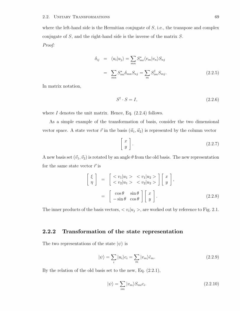
2.2. Unitary Transformations 69
where the left-hand side is the Hermitian conjugate of S, i.e., the transpose and complex
conjugate of S, and the right-hand side is the inverse of the matrix S.
Proof:
δij = 〈ui|uj〉 =∑
mn
S∗mi〈vm|vn〉Snj
=∑
mn
S∗miδmnSnj =
∑
m
S†imSmj. (2.2.5)
In matrix notation,
S† · S = I, (2.2.6)
where I denotes the unit matrix. Hence, Eq. (2.2.4) follows.
As a simple example of the transformation of basis, consider the two dimensional
vector space. A state vector r in the basis (u1, u2) is represented by the column vector
[xy
]
. (2.2.7)
A new basis set (v1, v2) is rotated by an angle θ from the old basis. The new representation
for the same state vector r is
[ξη
]
=
[< v1|u1 > < v1|u2 >< v2|u1 > < v2|u2 >
] [xy
]
,
=
[cos θ sin θ− sin θ cos θ
] [xy
]
. (2.2.8)
The inner products of the basis vectors, < vi|uj >, are worked out by reference to Fig. 2.1.
2.2.2 Transformation of the state representation
The two representations of the state |ψ〉 is
|ψ〉 =∑
i
|ui〉ci =∑
m
|vm〉cm. (2.2.9)
By the relation of the old basis set to the new, Eq. (2.2.1),
|ψ〉 =∑
im
|vm〉Smici. (2.2.10)
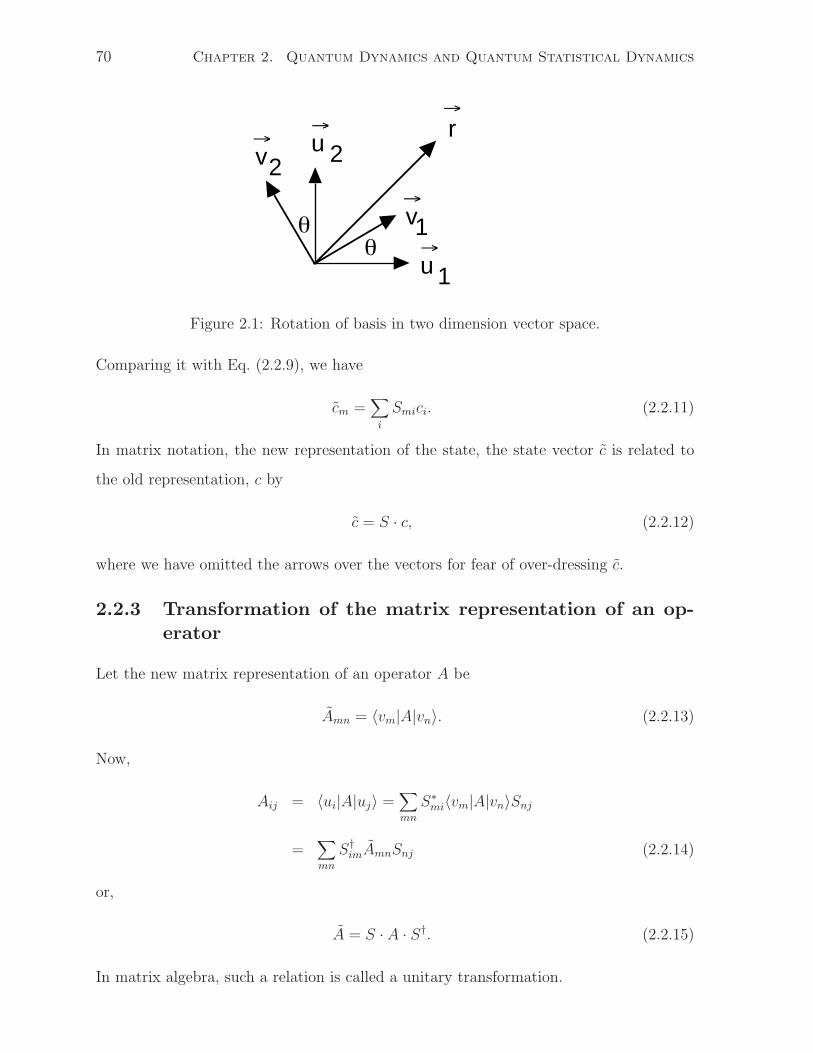
uv
1
2r→
→→
v→
2
1
u→θ
θ
70 Chapter 2. Quantum Dynamics and Quantum Statistical Dynamics
Figure 2.1: Rotation of basis in two dimension vector space.
Comparing it with Eq. (2.2.9), we have
cm =∑
i
Smici. (2.2.11)
In matrix notation, the new representation of the state, the state vector c is related to
the old representation, c by
c = S · c, (2.2.12)
where we have omitted the arrows over the vectors for fear of over-dressing c.
2.2.3 Transformation of the matrix representation of an op-erator
Let the new matrix representation of an operator A be
Amn = 〈vm|A|vn〉. (2.2.13)
Now,
Aij = 〈ui|A|uj〉 =∑
mn
S∗mi〈vm|A|vn〉Snj
=∑
mn
S†imAmnSnj (2.2.14)
or,
A = S · A · S†. (2.2.15)
In matrix algebra, such a relation is called a unitary transformation.
2.2. Unitary Transformations 71
2.2.4 Invariance under a unitary transformation
The following properties are invariant after a unitary transformation:
1. Inner product between two states |ψ〉 and |φ〉
〈ψ|φ〉 = c † · d, (2.2.16)
where c and d are the vector representations of |ψ〉 and |φ〉.
2. Eigenvalues of an operator.
3. Operator relations.
2.2.5 Diagonalization of a Hermitian operator
Suppose a Hermitian operator A has a complete set of orthonormal eigenstates |ψi〉with eigenvalues αi. We may choose to use the eigenstates of A as the basis set. Then
the matrix of A is a diagonal matrix Λ with elements αiδij.
If we start off with representation in a basis set which are not eigenstates of A, the
unitary transformation is found by solving for the eigenvectors and the eigenvalues of the
matrix A:
A · c i = αici. (2.2.17)
The transformation matrix which diagonalizes A is formed by the column vectors c i:
S† = [c 1 c 2 c 3 . . .], (2.2.18)
i.e.,
SAS† = Λ =
α1 0 . . .0 α2 . . .. . . . . . . . .
. (2.2.19)
In particular, the matrix method to solve the time-independent Schrodinger equation
is to find the matrix representation of the Hamiltonian H in some basis set and then
to diagonalize the matrix H, i.e. find the eigenvectors and eigenvalues of the matrix H.
With modern high speed computers, this method is much used for atomic and molecular
calculations.
72 Chapter 2. Quantum Dynamics and Quantum Statistical Dynamics
In exactly the same way as the operators, the matrices can only be simultaneously
diagonalized by the same set of functions if and only if the matrices commute with one
another.
2.3 The Schrodinger and Heisenberg Representa-tions
2.3.1 The Schrodinger representation
In Schrodinger’s theory, to find the time dependence of a property of a system, one
solves the time-dependent Schrodinger equation for the wave function as a function of
time, from which the (statistical) knowledge of any property is obtained. In the abstract
form, The Schrodinger equation for the state vector is given by
H|Ψ(t)〉 = ih∂
∂t|Ψ(t)〉. (2.3.1)
It is easy to verified that, if H is independent of time, the formal solution is
|Ψ(t)〉 = e−iHt/h |Ψ(0)〉. (2.3.2)
The time evolution of a state from time t0 to time t may be regarded as a unitary
transformation (called the evolution operator):
|Ψ(t)〉 = U(t − t0) |Ψ(t0)〉,
U(t − t0) = e−ih
H(t−t0). (2.3.3)
In the chapters on collision theory and on the time-dependent perturbation, the time
evolution of a state governed by a time-dependent Hamiltonian will be studied. The
unitary transformation preserves the length of the state vector 〈Ψ(t)|Ψ(t)〉 and, hence,
the total probability is constant in time.
The eigenstates |ψn〉 of the time-independent Hamiltonian H with eigenvalues En
form a special basis set. Under it, the matrix representation of the evolution operator is
diagonal,
Umn(t) = δm,ne−iEnt/h. (2.3.4)
2.3. The Schrodinger and Heisenberg Representations 73
At time t, the state |Ψ(t)〉 is represented by
|Ψ(t)〉 =∑
n
|ψn〉cn(t), (2.3.5)
where
cn(t) = e−iEnt/h cn(0). (2.3.6)
The time dependence of the expectation value of an operator A is given by:
〈A〉t = 〈Ψ(t)|A|Ψ(t)〉 =∑
m,n
c ∗m (0)Am,ncn(0)ei(Em−En)t/h. (2.3.7)
Aside from any explicit time dependence of the operator A itself, the time development
of the mean value of A is expressed through the oscillatory factors ei(Em−En)t/h.
2.3.2 The Heisenberg representation
Consider the unitary transformation from any time-independent basis:
S = eiHt/h. (2.3.8)
The representation with respect to the new set of basis is called the Heisenberg repre-
sentation. The transformed state for the state vector at time t,
|Ψ〉 = S|Ψ(t)〉 = |Ψ(0)〉, (2.3.9)
is independent of time. On the other hand, the matrix representation of an operator is
A = S · A · S† = eiHt/hAe−iHt/h, (2.3.10)
which changes with time in addition to any possible explicit time dependence of the
operator A.
2.3.3 Equation of motion for an observable in the Heisenbergrepresentation
d
dtA =
i
h
[HeiHt/hAe−iHt/h − eiHt/hAe−iHt/hH
]+ eiHt/h
∂A
∂t
e−iHt/h
=i
h[H, A] +
∂A
∂t. (2.3.11)
74 Chapter 2. Quantum Dynamics and Quantum Statistical Dynamics
In the last term, it is understood that the time derivative is with respect to the explicit
time dependence of the operator A.
The matrix form of the equation of motion is
dA
dt=
i
h[H, A] +
∂A
∂t. (2.3.12)
In the Hamiltonian formulation of classical mechanics, the Hamiltonian H(q, p) and any
property A(q, p, t) are functions of the generalized coordinates q and their canonical
conjugates p and time t. The equation of motion for A is
dA
dt=
∂A
∂p· dp
dt+
∂A
∂q
dq
dt+
∂A
∂t
=∂A
∂q
∂H
∂p− ∂A
∂p
∂H
∂q+
∂A
∂t
≡ −H, A +∂A
∂t. (2.3.13)
The bracket in the last line is known as the Poisson bracket. Notice the parallel forms of
the quantum mechanical equation (2.3.12) and of the classical counterpart, Eq. (2.3.13).
Indeed, in Heisenberg’s version of quantum mechanics, known also as the matrix mechan-
ics, he constructed the quantum equation of motion by replacing the Poisson bracket in
the classical equation of motion by −i/h times the commutation bracket and regarding
the dynamical variables as matrices. The equivalence of the Schrodinger version and the
Heisenberg version of quantum mechanics is thus demonstrated by deriving the latter
from the former.
2.3.4 Matrix mechanics of a particle
Consider a particle of mass m in a potential V .
H = P 2/2m + V (R ). (2.3.14)
The operator X now stands for the position observable in the Heisenberg representation.
Since X has no explicit time dependence, its equation of motion is
dX
dt=
i
h[H, X] =
Px
m, (2.3.15)
2.4. Feynman Path Integral Method 75
where Px is the x-component of the momentum operator. We have used the commutation
rule
[Px, X] = −ih. (2.3.16)
Similarly,
dPx
dt=
i
h[H, Px] = −∂V
∂X. (2.3.17)
Here, the force is again an operator or a matrix in the Heisenberg representation.
2.4 Feynman Path Integral Method
The evolution operator in Eq. (2.3.3) is more than a formal solution of the Schrodinger
equation. In this section, we examine its physical meaning more closely by the concept
of propagator and the path integral method, both due to Feynman.
2.4.1 The Propagator
Consider the single particle case. Multiplying Eq. (2.3.2) from the left by the position
eigenstate 〈r |, we obtain the time evolution of the state wave function in the form:
Ψ(r, t) =∫
d3r′ U(r, r′, t − t′)Ψ(r′, t′), (2.4.1)
where the evolution operator U in spatial representation becomes the propagator,
U(r, r′, t − t′) = θ(t − t′)〈r|e−iH(t−t′)/h|r′〉. (2.4.2)
Note that the propagator is just the time evolution in the particle going from position r′
at time t′ to r at time t. We have inserted the step-function θ(t− t′) to denote causality.
In the terms of the theory of differential equations, the propagator is just the Green’s
function which satisfies the equation:[
ih∂
∂t− H
]
U(r, r′, t − t′) = ihδ(t − t′)δ3(r − r′), (2.4.3)
with the condition that U(r, r′, t − t′) vanishes for t < t′.
By using the plane-wave eigenstates, it is possible to evaluate the propagator for the
free particle (with the potential energy V = 0) in one dimension (Problem 7):
U(x − x′, t − t′) =
√m
2πih(t − t′)exp
[im(x − x′)2
2h(t − t′)
]
. (2.4.4)
You may recognize this from the heat diffusion except for the factor of i in the time.
76 Chapter 2. Quantum Dynamics and Quantum Statistical Dynamics
2.4.2 The Path Integral
We shall consider the one-dimension system. Generalization of the formulation is straight-
forward. The path integral method gives an expression for the propagator in the following
way:
1. Consider all possible paths from the point (x0, t0) to (xf , tf ).
2. Find the action S[x(t)] along each path C : x = x(t).
3. The propagator is proportional to the sum over all possible paths of the exponential,
expiS[x(t)]/h.
The action is the classical quantity of the integral along the path of the Lagrangian L:
S =∫
Cdt L =
∫
Cdt
m
2
(dx
dt
)2
− V (x)
. (2.4.5)
We break each path C : x = x(t) from (x0, t0) to (xf , tf ) into N segments with inter-
mediate points (xj, tj), j = 1, 2, . . . N and j = N coinciding with the final point. (See
Fig. 2.2). Take the time segments to be equal, tj − tj−1 = ∆t. Then the sum over all
paths is given by
N∏
j=1
∫
dxj
N∏
n=1
eiS(tn,tn−1)/h, (2.4.6)
which, in the limit of infinite N , is called a functional integral:
U(xf , x0, tf − t0) =∫ xf
x0
D[x(t)]ei∫
CdtL/h, (2.4.7)
where the constant of proportionality is incorporated into the metric of the integration
(see below).
The functional integral expression for the propagator may be derived by considering
the propagator as the overlap integral:
U(x, x′, t − t′) = 〈x, t|x′, t′〉. (2.4.8)
Along all the possible paths broken up into N segments,
U(xf , x0, tf − t0) =
N∏
j=1
∫
dxj
〈xN , tN |xN−1, tN−1〉〈xN−1, tN−1|xN−2, tN−2〉
. . . 〈x1, t1|x0, t0〉. (2.4.9)
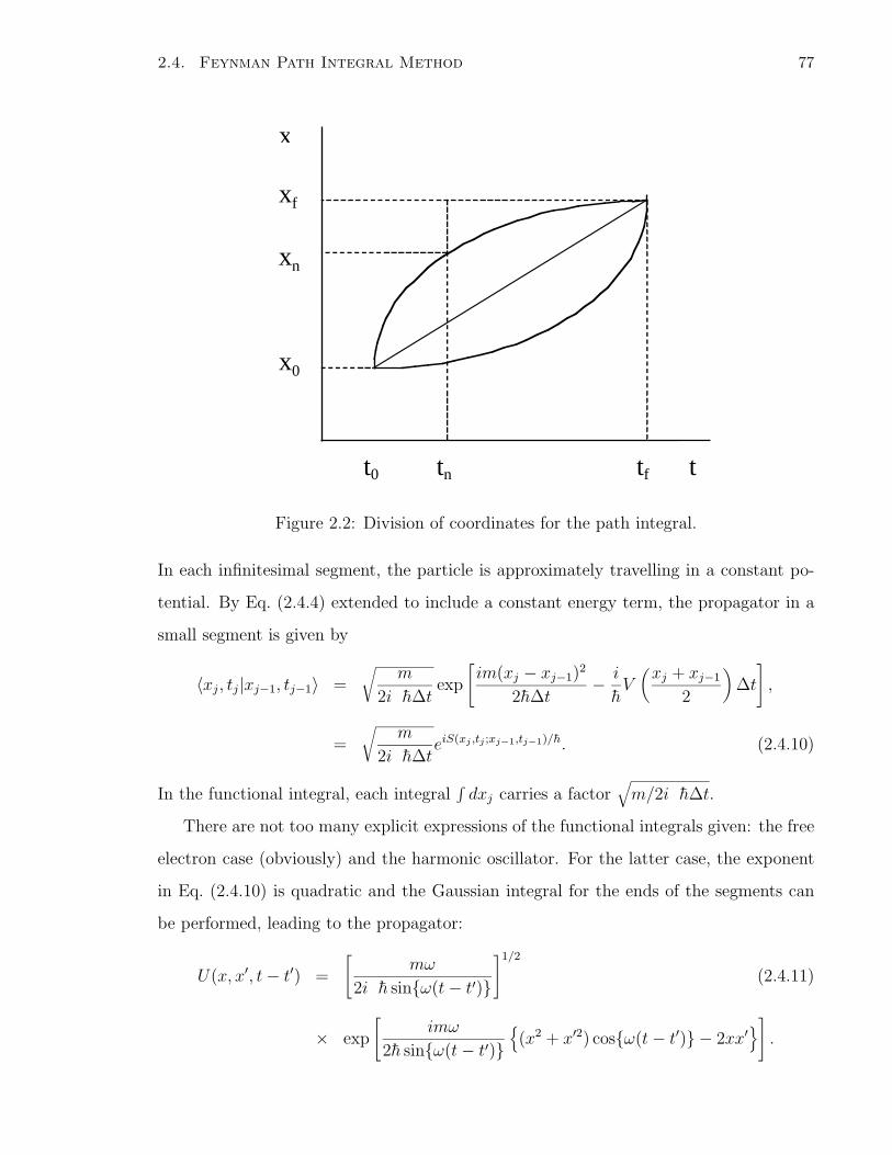
t0
x0
xn
tn tf
xf
x
t
2.4. Feynman Path Integral Method 77
Figure 2.2: Division of coordinates for the path integral.
In each infinitesimal segment, the particle is approximately travelling in a constant po-
tential. By Eq. (2.4.4) extended to include a constant energy term, the propagator in a
small segment is given by
〈xj, tj|xj−1, tj−1〉 =
√m
2πih∆texp
[im(xj − xj−1)
2
2h∆t− i
hV
(xj + xj−1
2
)
∆t
]
,
=
√m
2πih∆teiS(xj ,tj ;xj−1,tj−1)/h. (2.4.10)
In the functional integral, each integral∫
dxj carries a factor√
m/2πih∆t.
There are not too many explicit expressions of the functional integrals given: the free
electron case (obviously) and the harmonic oscillator. For the latter case, the exponent
in Eq. (2.4.10) is quadratic and the Gaussian integral for the ends of the segments can
be performed, leading to the propagator:
U(x, x′, t − t′) =
[mω
2πih sinω(t − t′)
]1/2
(2.4.11)
× exp
[imω
2h sinω(t − t′)(x2 + x′2) cosω(t − t′) − 2xx′
]
.
78 Chapter 2. Quantum Dynamics and Quantum Statistical Dynamics
The significance of the path integral formulation is that it is an alternative to the
Schrodinger equation and that it is closer to the Hamilton-Jacobi formulation of New-
tonian mechanics. Thus, studying the classical limit of the quantum theory is easier.
It is readily generalized to many-body systems and fields and is, thus, a powerful tool
in statistical mechanics and field theory. The path nature is also useful in studying the
interference phenomena along different paths, such as the Bohm-Aharonov effect in a
mesoscopic metallic ring which has been observed recently. (See Chapter 9.)
2.5 Mixed Ensembles and Density Matrix
In determining the time evolution of a quantum system, we have so far assumed that the
initial state of the system is known. For an ensemble of identical quantum systems, such
as a beam of atoms, the initial states may not be known precisely but may be known
statistically. How do we describe the state of such an ensemble and its time evolution?
In examining the quantum mechanics of such an ensemble, we start with a probability
distribution among possible states for the systems in the ensemble. By dissecting the
possible differences between two ensembles in which each system has the same probability
of distribution among a set of basis states, we shall find situations where the quantum
state of one system is inadequate in representing a state of the whole ensemble. This
inadequacy illustrates the difference between the classical statistical distribution over
states for systems of an ensemble and the quantum nature of a linear combination of
states. It will be used to motivate the density matrix as a tool which utilizes the states of
a single system to represent all possible states of the ensemble. In the literature, density
matrix is also called density operator. We shall not use the latter nomenclature to avoid
confusion with the density operator used in the many-body theory in later chapters.
2.5.1 Pure and mixed ensembles
Consider a one-dimension system of a particle bound in a square well with only two
bound states (Fig. 2.3). Denote the ground state with even parity by |+〉 and the excited
state with odd parity by |−〉. There is an ensemble of a large number N of identical
copies of this system (which are isolated from one another). Half of them are in the even
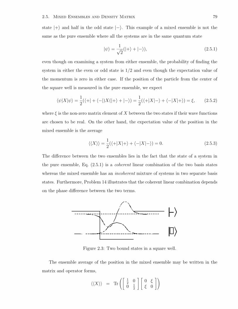
|+⟩
|−⟩
2.5. Mixed Ensembles and Density Matrix 79
state |+〉 and half in the odd state |−〉. This example of a mixed ensemble is not the
same as the pure ensemble where all the systems are in the same quantum state
|ψ〉 =1√2(|+〉 + |−〉), (2.5.1)
even though on examining a system from either ensemble, the probability of finding the
system in either the even or odd state is 1/2 and even though the expectation value of
the momentum is zero in either case. If the position of the particle from the center of
the square well is measured in the pure ensemble, we expect
〈ψ|X|ψ〉 =1
2(〈+| + 〈−|)X(|+〉 + |−〉) =
1
2(〈+|X|−〉 + 〈−|X|+〉) = ξ, (2.5.2)
where ξ is the non-zero matrix element of X between the two states if their wave functions
are chosen to be real. On the other hand, the expectation value of the position in the
mixed ensemble is the average
〈〈X〉〉 =1
2(〈+|X|+〉 + 〈−|X|−〉) = 0. (2.5.3)
The difference between the two ensembles lies in the fact that the state of a system in
the pure ensemble, Eq. (2.5.1) is a coherent linear combination of the two basis states
whereas the mixed ensemble has an incoherent mixture of systems in two separate basis
states. Furthermore, Problem 14 illustrates that the coherent linear combination depends
on the phase difference between the two terms.
Figure 2.3: Two bound states in a square well.
The ensemble average of the position in the mixed ensemble may be written in the
matrix and operator forms,
〈〈X〉〉 = Tr
([12
00 1
2
] [0 ξξ 0
])
80 Chapter 2. Quantum Dynamics and Quantum Statistical Dynamics
= Tr(
|+〉12〈+| + |−〉1
2〈−|
)
X
= Tr(ρX), (2.5.4)
where the operator
ρ =(
|+〉12〈+| + |−〉1
2〈−|
)
, (2.5.5)
is a description of the state of the mixed ensemble and is called the density matrix (or
density operator, though the latter can be confused with the same term used for density
in a many-particle system). The density matrix for the pure-state ensemble above is
given by
ρ =1
2(|+〉 + |−〉)(〈+| + 〈−|), (2.5.6)
with the matrix representation[
12
12
12
12
]
, (2.5.7)
in contrast with the diagonal matrix for the mixed ensemble. The off-diagonal term in
the density matrix is sometimes described as the coherence (between the two basis states)
in the ensemble. A special case of a mixed ensemble whose density matrix is a constant
times the identity operator would, of course, have no off-diagonal matrix elements in any
basis set and is known as an incoherent mixture. For more discussions of the off-diagonal
matrix elements, see Problem 8.
2.5.2 Density Matrix
In general, if the distribution of the systems in a ensemble can be expressed as a fraction
wj in each state |j〉 of a complete set of orthogonal states, the expectation value (called
the ensemble average) of a system property A is then
〈〈A〉〉 =∑
j
wj〈j|A|j〉, (2.5.8)
∑
j
wj = 1, (2.5.9)
where the double angular brackets connote first the quantum mechanical average over
the state of the system and then the average over the systems of the ensemble with the
2.5. Mixed Ensembles and Density Matrix 81
weighting factor wj. An important example is an ensemble in thermal equilibrium, where
wj ∝ e−Ej/kBT is the thermal distribution of the energy states at temperature T , kB being
the Boltzmann constant.
Now let us separate the average into two components: the physical observable A and
the state of the ensemble as characterized by the density matrix,
ρ =∑
j
|j〉wj〈j|. (2.5.10)
The ensemble average may be rewritten concisely as
〈〈A〉〉 = Tr(ρA), (2.5.11)
where Tr denotes trace of a matrix of the operator in any basis. A few simple properties
are easily proved:
1. ρ is hermitian.
2. Tr(ρ) = 1.
3. Tr(ρ2) ≤ 1.
The pure ensemble is a special case in which every system is in the same state, say
|k〉, i.e., wk = 1. Then,
ρ2 = ρ. (2.5.12)
2.5.3 Time evolution of an ensemble
In the Schrodinger representation, from the time evolution of the states
|j(t)〉 = e−iHt/h|j〉, (2.5.13)
the time dependence of the density matrix is
ρ(t) = e−iHt/hρeiHt/h. (2.5.14)
This leads to the time evolution equation for the density matrix, known as the Liouville
equation,
ih∂ρ(t)
∂t= [H, ρ(t)]. (2.5.15)
82 Chapter 2. Quantum Dynamics and Quantum Statistical Dynamics
As a pure ensemble evolves with time, it remains a pure ensemble.
The time dependence of the ensemble average of a property A is
〈〈A(t)〉〉 = Tr[ρ(t)A]. (2.5.16)
In the Heisenberg representation, the state vectors and hence the density matrix have no
explicit time dependence but the physical observable is given the time dependence,
A(t) = eiHt/hAe−iHt/h. (2.5.17)
Note the difference with the expression for ρ(t) in the Schrodinger representation and,
hence, also the difference in the Heisenberg equation of motion for A with that of ρ. The
time dependence of the average
〈〈A(t)〉〉 = Tr[ρA(t)] = Tr[ρ(t)A], (2.5.18)
since Tr(ABC) = Tr(BCA). (2.5.19)
2.6 Dissipative Processes in Quantum Dynamics
We have so far considered a system with a Hamiltonian which is a Hermitian operator.
Consequently, the evolution operator on any state is unitary. The quantum dynamics
conserves the norm of the state and the energy. In particular, if the system is in an
energy eigenstate, it will always be in that state albeit with a phase change. There are
observed processes which either do not conserve energy or particle number and which
are irreversible. We give a number of important examples below. These fall outside the
unitary evolution. We begin the study of such quantum processes by first making the
distinction between the closed system which obeys the quantum Hamiltonian dynamics
and the open system which can exhibit the dissipative processes. We set up the framework
for the study of an open system by making a larger closed system which contains the
open system. We leave to later chapters the study of the quantum dynamics of the larger
system and how the dissipative processes of the smaller open system arise. Instead, we
introduce here a phenomenological theory which can be used to describe a number of
common relaxation processes, frequently restricted to weak coupling to the outside of
the open system.
2.6. Dissipative Processes in Quantum Dynamics 83
The subject of the dissipative processes, also known under the rubric of “decoher-
ence”, is active and controversial. It is becoming of ever greater importance as the single
microscopic systems assume a more prominent role in scientific research and device devel-
opment. Further reading is highly recommended. Weiss’s [3] book gives a comprehensive
and up-to-date treatise of the subject. In this book, the central tool is the functional
integral (see Sec. 2.4). A good alternative is the book by Gardiner and Zoller [4]. The
dissipative phenomena have been treated for a long time, especially in spin resonances
[5] and in quantum optics [6, 7, 8, 9].
2.6.1 Examples of dissipative processes
There are many examples of systems which do not apparently behave like the conservative
Hamiltonian system.
1. In Chapter 11, we shall study the energy levels of the electron in a hydrogen atom.
The electron in an appropriate excited state of the hydrogen atom may decay to
the ground state with the spontaneous emission of a photon (a quantum of light)
with a mean time of the order τ ∼10 ns. This gives an energy uncertainty Γ = h/τ
known as the radiation linewidth of the energy level of the order 10−7 eV. Since
the ratio of the transition energy (of the order 10 eV) to Γ is 108, there is a period
of time much shorter than the radiative lifetime τ within which the state obeys
the unitary evolution quite accurately. For dynamics in time of the order of the
radiative time or longer, the decay of the energy eigenstate must be accounted for.
2. Under an electric field, while the electron in the ground state of the hydrogen
atom may have a negligible probability of tunneling out of the confining Coulomb
potential, the electron in a highly excited state could tunnel out in a finite time.
The escape represents another type of decay of the excited state.
3. In Gamow’s model of alpha decay of a nucleus, alpha particles (each being a compos-
ite particle with two neutrons and two protons) are trapped in a nuclear potential
of the form in Fig. 2.4. The wave function of the bound state at energy En can
tunnel out of the potential barrier.
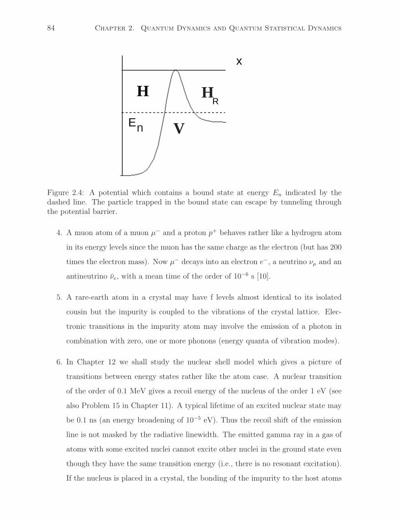
RH
V
H
nE
x
84 Chapter 2. Quantum Dynamics and Quantum Statistical Dynamics
Figure 2.4: A potential which contains a bound state at energy En indicated by thedashed line. The particle trapped in the bound state can escape by tunneling throughthe potential barrier.
4. A muon atom of a muon µ− and a proton p+ behaves rather like a hydrogen atom
in its energy levels since the muon has the same charge as the electron (but has 200
times the electron mass). Now µ− decays into an electron e−, a neutrino νµ and an
antineutrino νe, with a mean time of the order of 10−6 s [10].
5. A rare-earth atom in a crystal may have f levels almost identical to its isolated
cousin but the impurity is coupled to the vibrations of the crystal lattice. Elec-
tronic transitions in the impurity atom may involve the emission of a photon in
combination with zero, one or more phonons (energy quanta of vibration modes).
6. In Chapter 12 we shall study the nuclear shell model which gives a picture of
transitions between energy states rather like the atom case. A nuclear transition
of the order of 0.1 MeV gives a recoil energy of the nucleus of the order 1 eV (see
also Problem 15 in Chapter 11). A typical lifetime of an excited nuclear state may
be 0.1 ns (an energy broadening of 10−5 eV). Thus the recoil shift of the emission
line is not masked by the radiative linewidth. The emitted gamma ray in a gas of
atoms with some excited nuclei cannot excite other nuclei in the ground state even
though they have the same transition energy (i.e., there is no resonant excitation).
If the nucleus is placed in a crystal, the bonding of the impurity to the host atoms
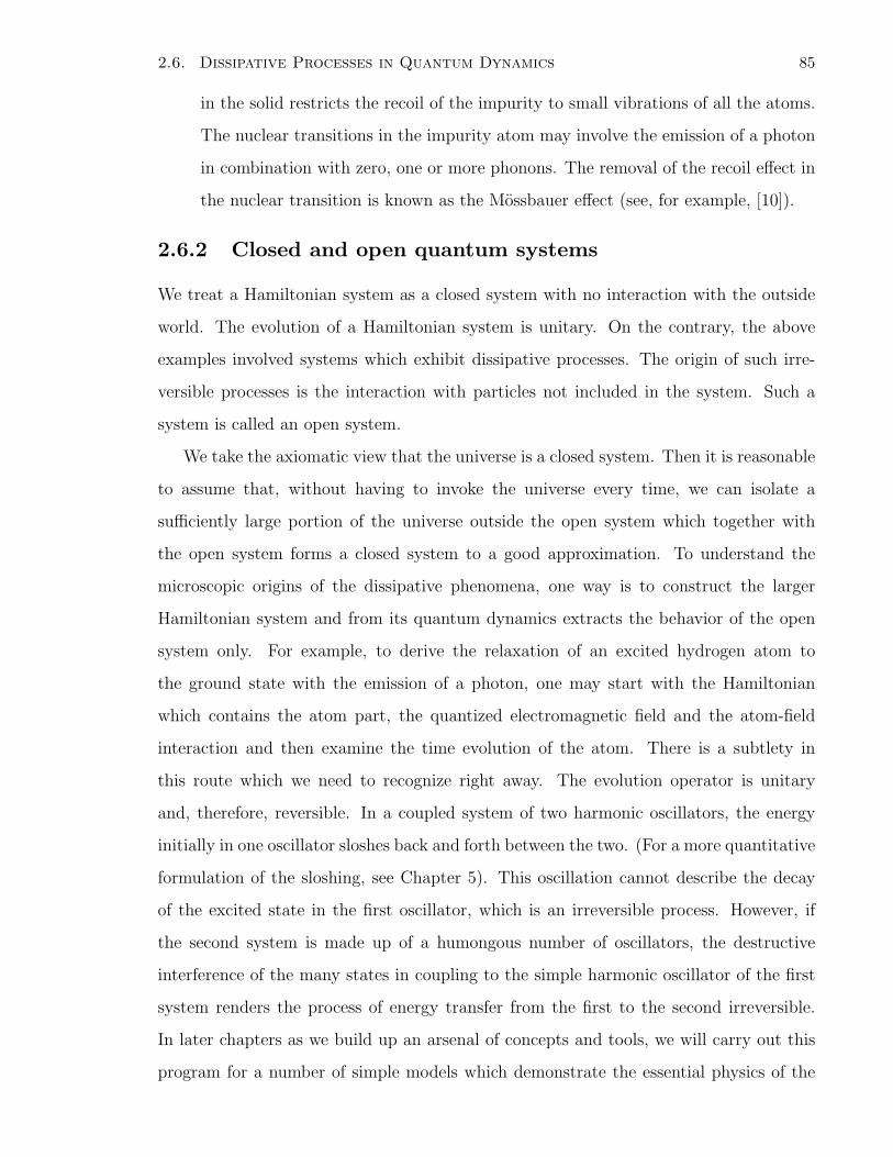
2.6. Dissipative Processes in Quantum Dynamics 85
in the solid restricts the recoil of the impurity to small vibrations of all the atoms.
The nuclear transitions in the impurity atom may involve the emission of a photon
in combination with zero, one or more phonons. The removal of the recoil effect in
the nuclear transition is known as the Mossbauer effect (see, for example, [10]).
2.6.2 Closed and open quantum systems
We treat a Hamiltonian system as a closed system with no interaction with the outside
world. The evolution of a Hamiltonian system is unitary. On the contrary, the above
examples involved systems which exhibit dissipative processes. The origin of such irre-
versible processes is the interaction with particles not included in the system. Such a
system is called an open system.
We take the axiomatic view that the universe is a closed system. Then it is reasonable
to assume that, without having to invoke the universe every time, we can isolate a
sufficiently large portion of the universe outside the open system which together with
the open system forms a closed system to a good approximation. To understand the
microscopic origins of the dissipative phenomena, one way is to construct the larger
Hamiltonian system and from its quantum dynamics extracts the behavior of the open
system only. For example, to derive the relaxation of an excited hydrogen atom to
the ground state with the emission of a photon, one may start with the Hamiltonian
which contains the atom part, the quantized electromagnetic field and the atom-field
interaction and then examine the time evolution of the atom. There is a subtlety in
this route which we need to recognize right away. The evolution operator is unitary
and, therefore, reversible. In a coupled system of two harmonic oscillators, the energy
initially in one oscillator sloshes back and forth between the two. (For a more quantitative
formulation of the sloshing, see Chapter 5). This oscillation cannot describe the decay
of the excited state in the first oscillator, which is an irreversible process. However, if
the second system is made up of a humongous number of oscillators, the destructive
interference of the many states in coupling to the simple harmonic oscillator of the first
system renders the process of energy transfer from the first to the second irreversible.
In later chapters as we build up an arsenal of concepts and tools, we will carry out this
program for a number of simple models which demonstrate the essential physics of the
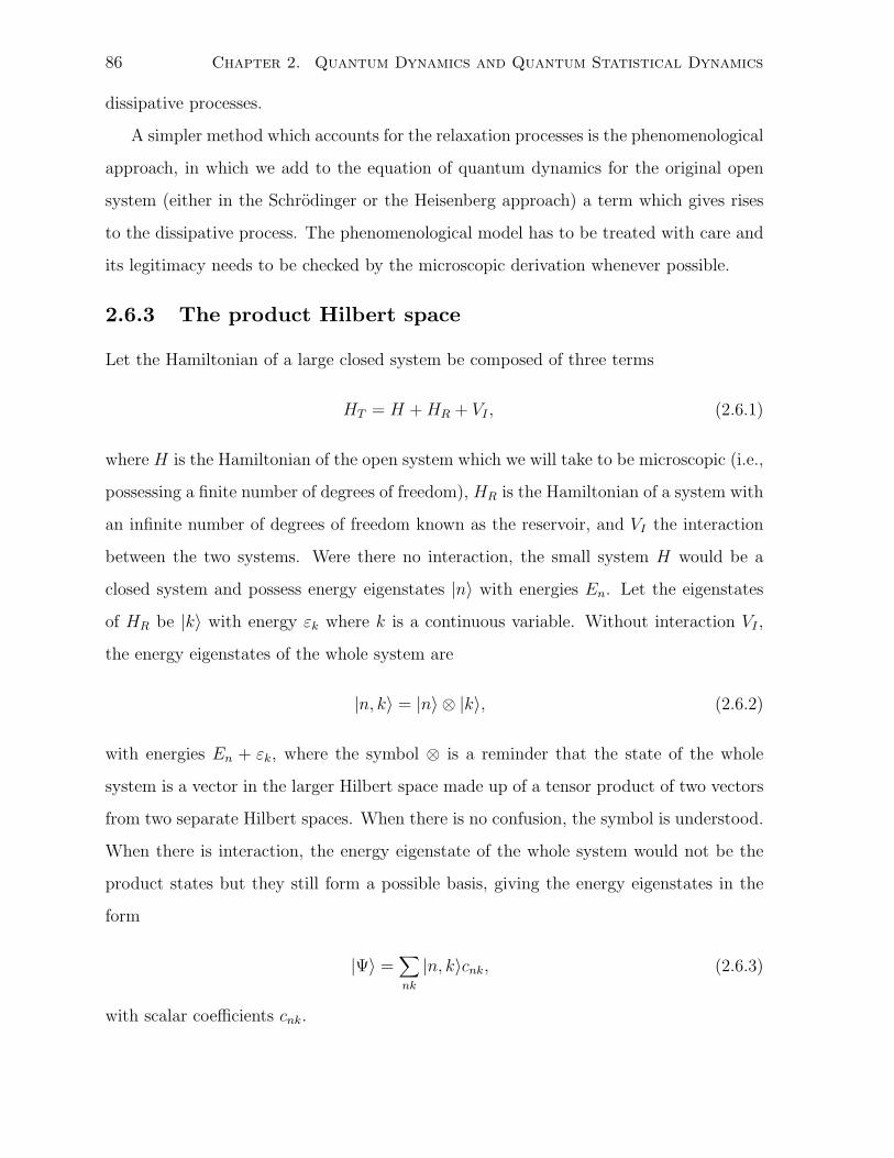
86 Chapter 2. Quantum Dynamics and Quantum Statistical Dynamics
dissipative processes.
A simpler method which accounts for the relaxation processes is the phenomenological
approach, in which we add to the equation of quantum dynamics for the original open
system (either in the Schrodinger or the Heisenberg approach) a term which gives rises
to the dissipative process. The phenomenological model has to be treated with care and
its legitimacy needs to be checked by the microscopic derivation whenever possible.
2.6.3 The product Hilbert space
Let the Hamiltonian of a large closed system be composed of three terms
HT = H + HR + VI , (2.6.1)
where H is the Hamiltonian of the open system which we will take to be microscopic (i.e.,
possessing a finite number of degrees of freedom), HR is the Hamiltonian of a system with
an infinite number of degrees of freedom known as the reservoir, and VI the interaction
between the two systems. Were there no interaction, the small system H would be a
closed system and possess energy eigenstates |n〉 with energies En. Let the eigenstates
of HR be |k〉 with energy εk where k is a continuous variable. Without interaction VI ,
the energy eigenstates of the whole system are
|n, k〉 = |n〉 ⊗ |k〉, (2.6.2)
with energies En + εk, where the symbol ⊗ is a reminder that the state of the whole
system is a vector in the larger Hilbert space made up of a tensor product of two vectors
from two separate Hilbert spaces. When there is no confusion, the symbol is understood.
When there is interaction, the energy eigenstate of the whole system would not be the
product states but they still form a possible basis, giving the energy eigenstates in the
form
|Ψ〉 =∑
nk
|n, k〉cnk, (2.6.3)
with scalar coefficients cnk.
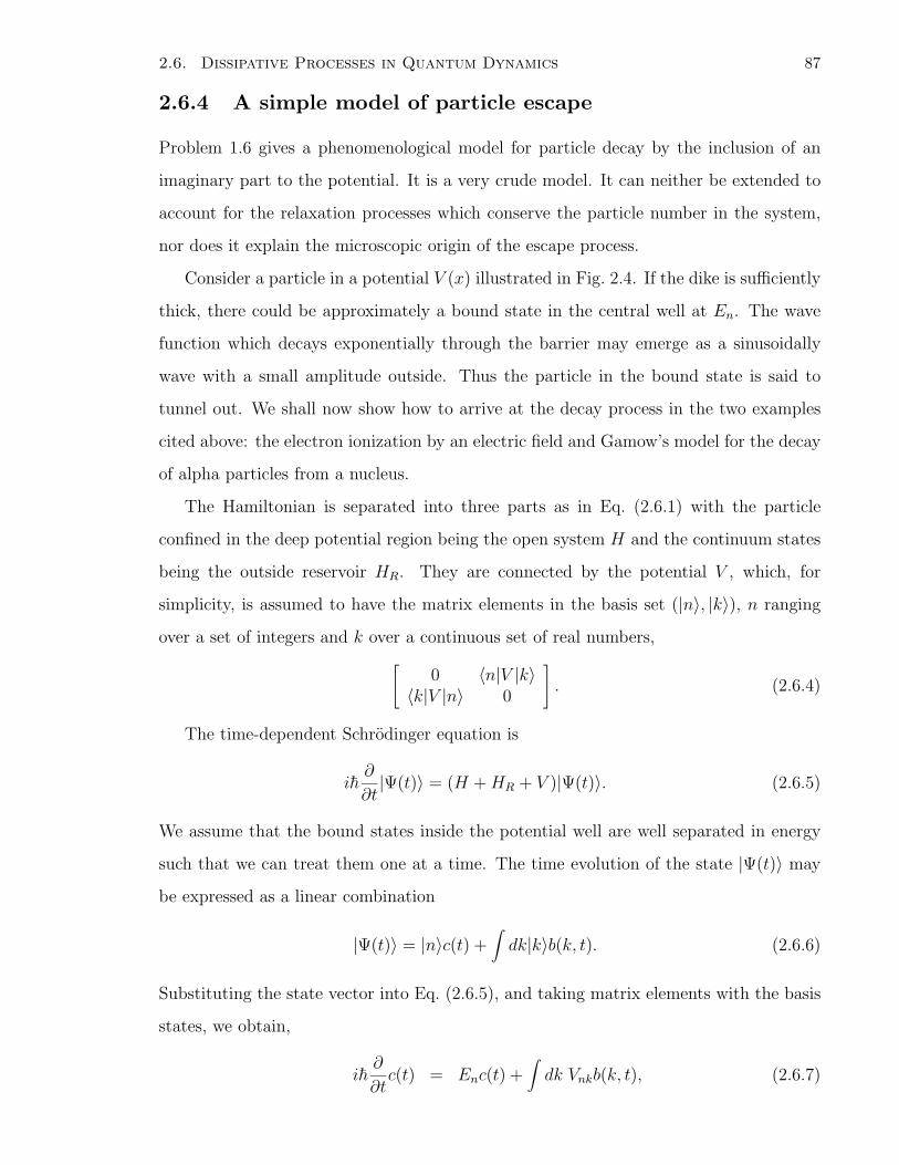
2.6. Dissipative Processes in Quantum Dynamics 87
2.6.4 A simple model of particle escape
Problem 1.6 gives a phenomenological model for particle decay by the inclusion of an
imaginary part to the potential. It is a very crude model. It can neither be extended to
account for the relaxation processes which conserve the particle number in the system,
nor does it explain the microscopic origin of the escape process.
Consider a particle in a potential V (x) illustrated in Fig. 2.4. If the dike is sufficiently
thick, there could be approximately a bound state in the central well at En. The wave
function which decays exponentially through the barrier may emerge as a sinusoidally
wave with a small amplitude outside. Thus the particle in the bound state is said to
tunnel out. We shall now show how to arrive at the decay process in the two examples
cited above: the electron ionization by an electric field and Gamow’s model for the decay
of alpha particles from a nucleus.
The Hamiltonian is separated into three parts as in Eq. (2.6.1) with the particle
confined in the deep potential region being the open system H and the continuum states
being the outside reservoir HR. They are connected by the potential V , which, for
simplicity, is assumed to have the matrix elements in the basis set (|n〉, |k〉), n ranging
over a set of integers and k over a continuous set of real numbers,
[0 〈n|V |k〉
〈k|V |n〉 0
]
. (2.6.4)
The time-dependent Schrodinger equation is
ih∂
∂t|Ψ(t)〉 = (H + HR + V )|Ψ(t)〉. (2.6.5)
We assume that the bound states inside the potential well are well separated in energy
such that we can treat them one at a time. The time evolution of the state |Ψ(t)〉 may
be expressed as a linear combination
|Ψ(t)〉 = |n〉c(t) +∫
dk|k〉b(k, t). (2.6.6)
Substituting the state vector into Eq. (2.6.5), and taking matrix elements with the basis
states, we obtain,
ih∂
∂tc(t) = Enc(t) +
∫
dk Vnkb(k, t), (2.6.7)
88 Chapter 2. Quantum Dynamics and Quantum Statistical Dynamics
ih∂
∂tb(k, t) = Vknc(t) + εkb(k, t), (2.6.8)
where Vnk = 〈n|V |k〉. (2.6.9)
The coupled set of differential equations may be simplified by the transformation,
c(t) = e−iEnt/hc(t), (2.6.10)
b(k, t) = e−iεkt/hb(k, t), (2.6.11)
where Vnk(t) = 〈n|V |k〉ei(En−εk)t/h. (2.6.12)
The substitution is known as the interacting representation (see Section 5.6). The resul-
tant equations are
ih∂
∂tc(t) =
∫
dk Vnk(t)b(k, t), (2.6.13)
ih∂
∂tb(k, t) = Vkn(t)c(t), (2.6.14)
where Vkn(t) = [Vnk(t)]∗. (2.6.15)
We make the first key assumption that initially t = t0, the state of the whole system is
given by the state |n〉 in the well with the reservior completely quiescent, i.e.,
c(t0) = e−iEnt0/h,
b(k, t) = 0. (2.6.16)
Then, from Eq. (2.6.14), the coefficient b(k, t) is an integral of c(t), which may be sub-
stituted into Eq. (2.6.13), yielding
ih∂
∂tc(t) = − i
h
∫ t
t0dt′
∫
dk |Vnk|2ei(En−εk)(t−t′)/hc(t′). (2.6.17)
We now make the second assumption that the coupling matrix element Vnk is weak.
Then the zeroth order solution of Eq. (2.6.13) has the rapidly oscillatory time dependence
with a period of 2πh/En and c(t) is slowly varying in time compared with the time of
h/En. This enable us to carry out the integral on the right of Eq. (2.6.17),
∫ t
t0dt′
∫
dk |Vnk|2ei(En−εk)(t−t′)/h, (2.6.18)
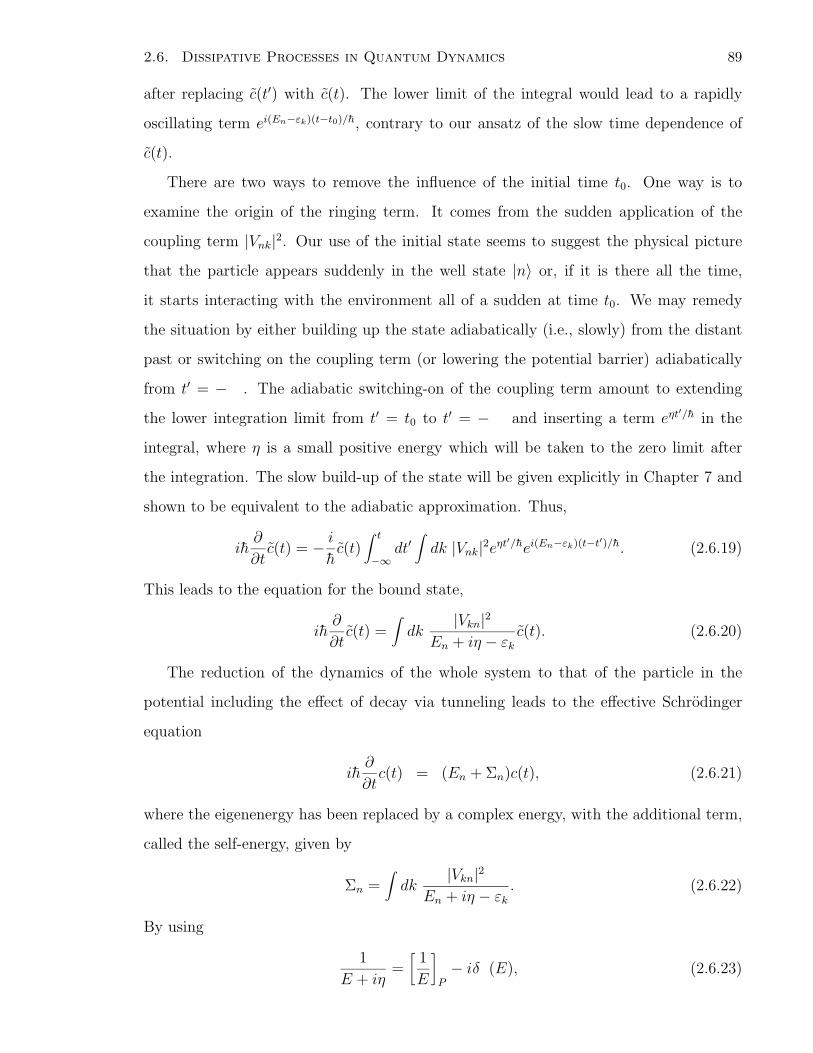
2.6. Dissipative Processes in Quantum Dynamics 89
after replacing c(t′) with c(t). The lower limit of the integral would lead to a rapidly
oscillating term ei(En−εk)(t−t0)/h, contrary to our ansatz of the slow time dependence of
c(t).
There are two ways to remove the influence of the initial time t0. One way is to
examine the origin of the ringing term. It comes from the sudden application of the
coupling term |Vnk|2. Our use of the initial state seems to suggest the physical picture
that the particle appears suddenly in the well state |n〉 or, if it is there all the time,
it starts interacting with the environment all of a sudden at time t0. We may remedy
the situation by either building up the state adiabatically (i.e., slowly) from the distant
past or switching on the coupling term (or lowering the potential barrier) adiabatically
from t′ = −∞. The adiabatic switching-on of the coupling term amount to extending
the lower integration limit from t′ = t0 to t′ = −∞ and inserting a term eηt′/h in the
integral, where η is a small positive energy which will be taken to the zero limit after
the integration. The slow build-up of the state will be given explicitly in Chapter 7 and
shown to be equivalent to the adiabatic approximation. Thus,
ih∂
∂tc(t) = − i
hc(t)
∫ t
−∞dt′
∫
dk |Vnk|2eηt′/hei(En−εk)(t−t′)/h. (2.6.19)
This leads to the equation for the bound state,
ih∂
∂tc(t) =
∫
dk|Vkn|2
En + iη − εk
c(t). (2.6.20)
The reduction of the dynamics of the whole system to that of the particle in the
potential including the effect of decay via tunneling leads to the effective Schrodinger
equation
ih∂
∂tc(t) = (En + Σn)c(t), (2.6.21)
where the eigenenergy has been replaced by a complex energy, with the additional term,
called the self-energy, given by
Σn =∫
dk|Vkn|2
En + iη − εk
. (2.6.22)
By using
1
E + iη=
[1
E
]
P− iπδ(E), (2.6.23)
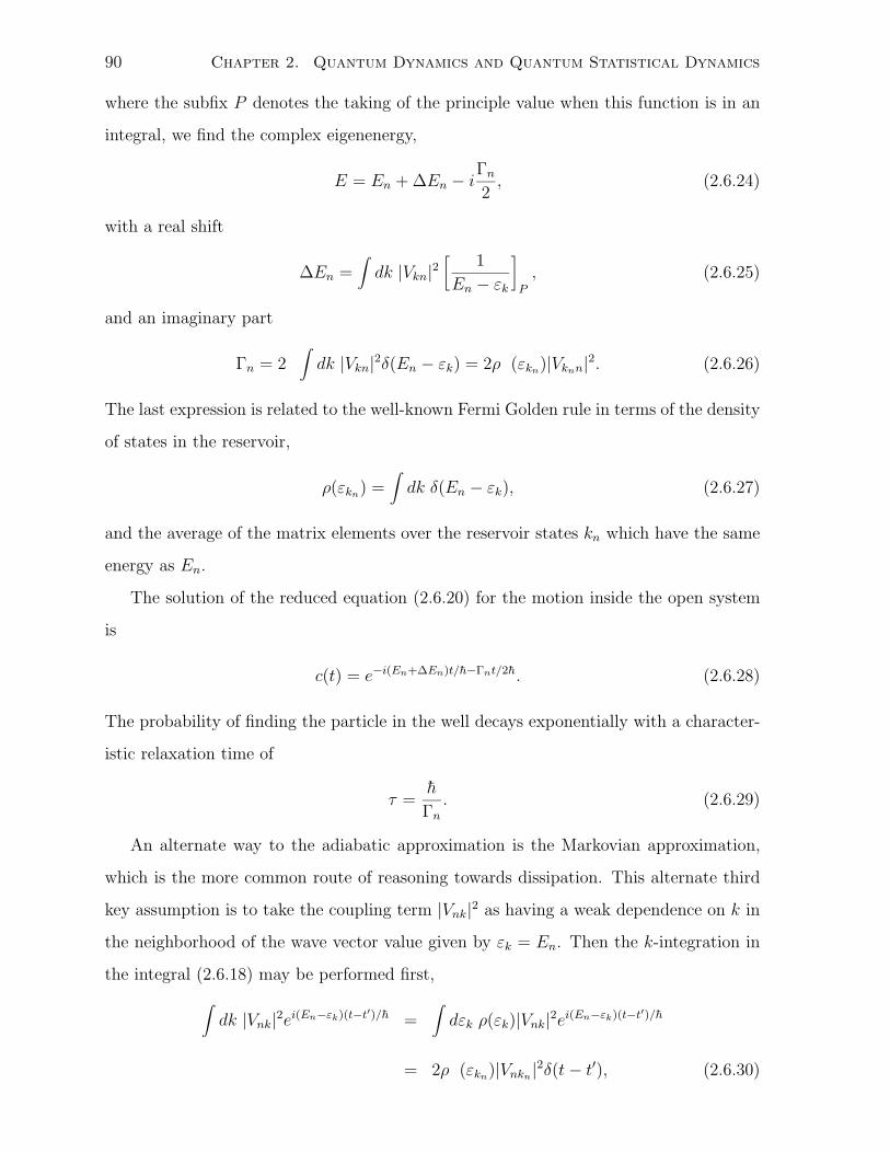
90 Chapter 2. Quantum Dynamics and Quantum Statistical Dynamics
where the subfix P denotes the taking of the principle value when this function is in an
integral, we find the complex eigenenergy,
E = En + ∆En − iΓn
2, (2.6.24)
with a real shift
∆En =∫
dk |Vkn|2[
1
En − εk
]
P
, (2.6.25)
and an imaginary part
Γn = 2π∫
dk |Vkn|2δ(En − εk) = 2πρ(εkn)|Vknn|2. (2.6.26)
The last expression is related to the well-known Fermi Golden rule in terms of the density
of states in the reservoir,
ρ(εkn) =∫
dk δ(En − εk), (2.6.27)
and the average of the matrix elements over the reservoir states kn which have the same
energy as En.
The solution of the reduced equation (2.6.20) for the motion inside the open system
is
c(t) = e−i(En+∆En)t/h−Γnt/2h. (2.6.28)
The probability of finding the particle in the well decays exponentially with a character-
istic relaxation time of
τ =h
Γn
. (2.6.29)
An alternate way to the adiabatic approximation is the Markovian approximation,
which is the more common route of reasoning towards dissipation. This alternate third
key assumption is to take the coupling term |Vnk|2 as having a weak dependence on k in
the neighborhood of the wave vector value given by εk = En. Then the k-integration in
the integral (2.6.18) may be performed first,
∫
dk |Vnk|2ei(En−εk)(t−t′)/h =∫
dεk ρ(εk)|Vnk|2ei(En−εk)(t−t′)/h
= 2πρ(εkn)|Vnkn|2δ(t − t′), (2.6.30)
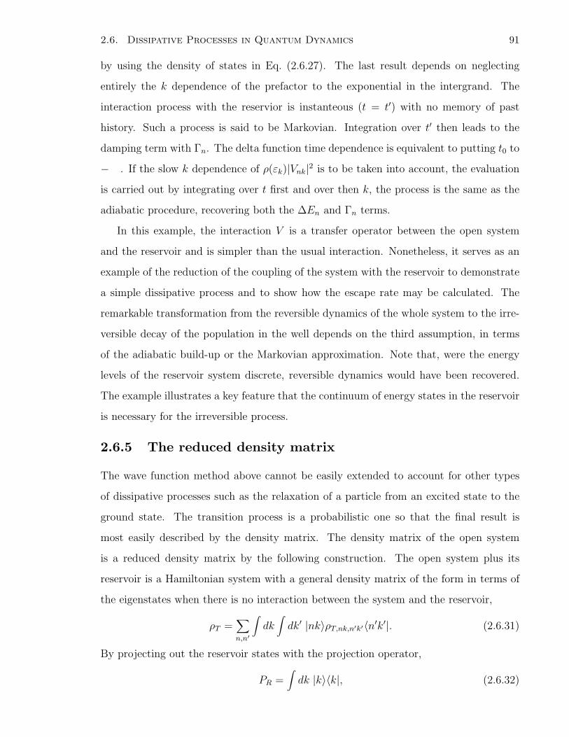
2.6. Dissipative Processes in Quantum Dynamics 91
by using the density of states in Eq. (2.6.27). The last result depends on neglecting
entirely the k dependence of the prefactor to the exponential in the intergrand. The
interaction process with the reservior is instanteous (t = t′) with no memory of past
history. Such a process is said to be Markovian. Integration over t′ then leads to the
damping term with Γn. The delta function time dependence is equivalent to putting t0 to
−∞. If the slow k dependence of ρ(εk)|Vnk|2 is to be taken into account, the evaluation
is carried out by integrating over t first and over then k, the process is the same as the
adiabatic procedure, recovering both the ∆En and Γn terms.
In this example, the interaction V is a transfer operator between the open system
and the reservoir and is simpler than the usual interaction. Nonetheless, it serves as an
example of the reduction of the coupling of the system with the reservoir to demonstrate
a simple dissipative process and to show how the escape rate may be calculated. The
remarkable transformation from the reversible dynamics of the whole system to the irre-
versible decay of the population in the well depends on the third assumption, in terms
of the adiabatic build-up or the Markovian approximation. Note that, were the energy
levels of the reservoir system discrete, reversible dynamics would have been recovered.
The example illustrates a key feature that the continuum of energy states in the reservoir
is necessary for the irreversible process.
2.6.5 The reduced density matrix
The wave function method above cannot be easily extended to account for other types
of dissipative processes such as the relaxation of a particle from an excited state to the
ground state. The transition process is a probabilistic one so that the final result is
most easily described by the density matrix. The density matrix of the open system
is a reduced density matrix by the following construction. The open system plus its
reservoir is a Hamiltonian system with a general density matrix of the form in terms of
the eigenstates when there is no interaction between the system and the reservoir,
ρT =∑
n,n′
∫
dk∫
dk′ |nk〉ρT,nk,n′k′〈n′k′|. (2.6.31)
By projecting out the reservoir states with the projection operator,
PR =∫
dk |k〉〈k|, (2.6.32)
92 Chapter 2. Quantum Dynamics and Quantum Statistical Dynamics
and taking the trace, we obtain the reduced density matrix of the system,
ρ = Tr[PRρT PR] = Tr[PRρT ] =∑
nn′|n〉
∫
dk ρT,nk,n′k〈n′|. (2.6.33)
The equation of motion for the density matrix of the whole system, the Liouville
equation, assumes the simple form,
∂
∂tρT = LT ρT , (2.6.34)
if the linear operator, the Liouville operator, associated with a Hamiltonian, is defined
generally by,
Lρ =1
ih[H, ρ]. (2.6.35)
Following a procedure similar in spirit to the wave function method to eliminate the
reservoir states in the preceding section, a Liouville equation for the reduced density
matrix is commonly obtained in the Redfield form [3, 5],
∂
∂tρn,m(t) = −iωnmρn,m(t) −
∑
k
Rnmkρk(t), (2.6.36)
where the transition frequency is given by
ωnm =En − Em
h. (2.6.37)
The explanation of the relaxation coefficients Rnmk has to await the development of
the microscopic theory in later chapters. Akin to the introduction of the adiabatic
switching-on which leads to the irreversible decay in the last subsection, the Redfield
result depends on the Born approximation (using weak coupling) and the Markovian
approximation, which has the same effect as the adiabatic approximation in reducing the
t − t′ dependence in the kernel of the integral in Eq. (2.6.19) to being an instantaneous
response in Eq.(2.6.20). The weak coupling limit and the Markovian approximation are
not necessary for the existence of an equation of motion for the reduced density matrix,
known as the master equation.
The time evolution of the density matrix to describe the dissipative dynamics and the
trace of the time-independent observable times the time-dependent density matrix as the
mean value of the observable constitute the analog to the Schrodinger representation. In
2.6. Dissipative Processes in Quantum Dynamics 93
the analog of the Heisenberg representation, the density matrix remains time independent
and the equation of motion of a physical observable would include both a damping term
involving the physical observable of the open system and a noise operator which is a
function of the relevant operators of the reservoir, known as the quantum Langevin
equation because of the correspondence with the classical Langevin equation used to treat
classical dissipative dynamics such as the Brownian motion. An introductory treatment
of the Heisenberg type approach will be given in later chapters.
2.6.6 Phenomenological approach to the relaxation dynamics
It is possible to add damping terms to the Liouville equation for the Hamilton of the
system to simulate the dissipative forces. However, it may leads to certain undesirable
results for the time development of the reduced density matrix. If the open system has
only relaxation transitions within the system, while the total energy is not conserved,
the total number of particles is conserved. Then the trace of the reduced density should
remain unity. A general form of the Liouville operator [11] which preserves the trace
of the reduce density matrix may be deduced by means of the concept of the dynamic
semigroup in terms of its generators. (See Chapter 8 for the concept of the group,
semigroup and generators [12].) Lindblad [13] has deduced a simple form,
∂
∂tρ(t) =
1
ih[H, ρ] +
1
2
∑
j
[Ljρ(t), L†
j] + [Lj, ρ(t)L†j]
, (2.6.38)
where Lj is a set of damping operators which act on the state of the open system. For
example, for linear coupling of a particle to a reservoir,
L = αX + iβP, (2.6.39)
where X and P are the position and momentum operators of the particle in an open
system and α and β are scalars. For some simple models of the system plus reservoir, it
is possible to derive the master equation and identify the Lindblad operators. It is clear
from the form of the Lindblad equation that both the weak coupling and the Markovian
approximation have been used.
An important example of the application of the Lindblad form of dissipative processes
is given by the transitions in a two-state system, of which we shall have a lot to say in
94 Chapter 2. Quantum Dynamics and Quantum Statistical Dynamics
Chapter 5. Let the ground state and excited state be |0〉 and |1〉. The Lindblad operator
which simulates the decay from the excited to the ground state with the emission of a
quantum of energy to the reservoir,
Le =√
hγ|0〉〈1|, (2.6.40)
leads to the relaxation rates,
d
dt
[ρ00 ρ01
ρ10 ρ11
]
=
[γρ11 −1
2γρ01
−12γρ10 −γρ11
]
. (2.6.41)
Note that the decay rate of the excited state population is exactly offset by the increase
in the ground state population. The interesting case of the off-diagonal elements ρ01, ρ10
known as coherences will be studied in Chapter 5.
A second Lindblad operator which simulates the excitation from the ground state to
the excited state by absorbing a quantum of energy from the reservoir,
La =√
hγ′|1〉〈0|, (2.6.42)
leads to the relaxation rates,
d
dt
[ρ00 ρ01
ρ10 ρ11
]
=
[−γ′ρ00 −1
2γ′ρ01
−12γ′ρ10 γ′ρ00
]
. (2.6.43)
A third one
Lf =√
2hγ∗|1〉〈1|, (2.6.44)
leads only to the destruction of the phase coherence between the two states,
d
dt
[ρ00 ρ01
ρ10 ρ11
]
=
[0 −γ∗ρ01
−γ∗ρ10 0
]
. (2.6.45)
The derivation of these results are left as problems. The emission term Le and the
absorption term La, in addition to altering the occupation numbers of the energy levels
irreversibly, also contribute to the destruction of the phase coherence between two states,
(ρ01 or ρ10), known as dephasing. The term Lf might be viewed as the fluctuation of the
energy state |1〉 because of the interaction with the reservoir and it contributes only to
the dephasing, leading to the decreasing of ρ01 and ρ10 without affecting the populations
of the energy levels. This type of dephasing is known as “pure” dephasing. Unlike the
2.6. Dissipative Processes in Quantum Dynamics 95
dephasing rates γ/2, γ′/2 which is related to the transition rates γ, γ′, the pure dephasing
rate γ∗ is not related to any decay rate.
A physical way to view this extension of the Liouville equation (2.6.34) to include
dissipative terms is to extend the definition of the Liouville operator from Eq. (2.6.35)
to accommodate the non-Hermitian Hamiltonian Hc as
Lρ =1
ih(Hcρ − ρH†
c ). (2.6.46)
If we take the complex Hamiltonian to be
Hc = H − ih
2
∑
j
L†jLj − iVo, (2.6.47)
where H is the Hamiltonian of the open system and Lj is the Lindblad operator and Vo
is a Hermitian operator, the equation of motion of the density matrix becomes
∂ρ
∂t=
1
ih[H, ρ] − 1
2
∑
j
L†jLj, ρ −
1
hVo, ρ, (2.6.48)
where A, B ≡ AB + BA is the anticommutation bracket. Both the Lindblad terms
and the imaginary potential term Vo lead to the decay of the particle number in the
open system. The Lindblad terms above represent the scattering of the particles out of
the open system into the reservoir. To preserve the particle number (i.e., Tr(ρ)), a term∑
j LjρL†j, representing the scattering of the particles into the open system, has to be
added to the right-hand side of the new Liouville equation. This gives the form of the
Lindblad equation (2.6.38).
The term Vo represents particle decay. In nuclear scattering, the phenomenological
imaginary potential −iVo is known as the optical potential. For example, an elastic
scattering experiment of a neutron against a target of He3 atoms may be regarded as
the potential scattering of a particle (see Chapter 7). However, it is possible for a He3
atom to absorb a neutron (to become He4). In principle, it is possible to construct
a scattering theory with a conservative Hamiltonian for four particles (two neutrons
and two protons) but it is more convenient to analyze the scattering data as a particle
scattering in a complex potential, with the imaginary part simulating the decay of the
one-particle open system. The simplification becomes more needed as the target atoms
get heavier. For a reservoir with an Avogadro number of degrees of freedom, the use of
the dissipative dynamics becomes necessary.
96 Chapter 2. Quantum Dynamics and Quantum Statistical Dynamics
2.7 Quantum Measurement
The development of the measurements and associated theories utilizing quantum optics
in the last two decades has greatly increased both the range of possible measurements
and our understanding of the quantum processes associated with the measurement [14,
15]. The recent experiments and theories in the mesoscopic regime with atoms transfer
between a scanning tunneling tip and a solid surface add to this body of knowledge
[16]. We shall bypass the actual microscopic processes which lead to the “collapse”
of the quantum state after a measurement. While it is somewhat analogous to the
dissipative process, it is a still an actively researched and somewhat controversial subject
and, therefore, beyond the scope of our purview. Instead, we follow the simplification of
the measurement processes to a set of postulates and examine some consequences thereof.
2.7.1 Von Neumann’s postulates
In Section 1.7.6, two postulates were made regarding the outcome of a measurement of
a physical observable A as one of the eigenvalues with an assigned probability and the
“collapse” of the state of the measured system to the associated eigenstate. Since the
density matrix is often the more appropriate description of the system in the mixed state
form, we describe the two postulates in terms of the development of the density matrix
ρ:
1. The outcome of a measurement of the observable A is one of its eigenvalue, α, with
the probability
P (α) = Tr(|α〉〈α|ρ), (2.7.1)
where |α〉 is the associated eigenstate.
2. At the end of the measurement, the density matrix describing the system becomes
ρ′ = |α〉〈α|.
2.7.2 Back action noise of a measurement
By the second postulate, the result of a measurement makes a drastic change to the state.
If repeated measurements of the same observable could be made instantly, then the same
2.7. Quantum Measurement 97
value of the observable would be obtained. However, in reality the repeated measurement
has to be made at a finite time later. Then the first measurement introduces noise (i.e.,
uncertainty) to the properties of the system which do not commute with the first observed
property. After a finite time, the uncertainties in these observables may impart noise to
a subsequent measurement of the first observable, i.e., the same eigenvalue which was
measured the first time would not be reproduced.
A simple example is provided by measuring the position of a free particle. Suppose
that, right after a measurement of the position coordinate x, instead of the system being
in the position eigenstate, the state can be modeled by the Gaussian wave function given
by Eq. (1.10.1). It has an amount of uncertainty ∆x(0) from the instrumental noise. Note
that the uncertainty in momentum is the minimum allowed by the uncertainty principle,
∆p(0) = h/2∆x(0). In practice the instrument noise could be much worse, caused by
the correlation part in Eq. (1.9.15). In any case, a measurement of position gives rise
to an uncertainty in momentum and therefore, an additional uncertainty in subsequent
displacement which is proportional to the momentum. From Eq. (1.10.8), we have the
uncertainty in position at time t after the measurement given by
[∆x(t)]2 = [∆x(0)]2 +(
t
m
)2
[∆p(0)]2. (2.7.2)
The time evolution of the uncertainty in position for a general state is given in Problem 15.
The above relation shows that, the more precise the initial measurement of position is,
the larger the subsequent uncertain is through the Heisenberg uncertainty in momentum.
Thus, the first measurement of position creates the uncertainty in momentum which acts
back on the system. Hence,
[∆x(t)]2 = [∆x(0)]2
1 +
(ht
2m∆x(0)2
)2
(2.7.3)
= [∆x(0)]2
(
1 − ht
2m∆x(0)2
)2
+ht
m∆x(0)2
≥ ht
m. (2.7.4)
Thus, a second measurement of X after a certain time will have a growing minimum
uncertainty.
98 Chapter 2. Quantum Dynamics and Quantum Statistical Dynamics
Such a quantum limitation as the uncertainty in position measurement is relevant
to highly sensitive measurements, such as the attempt to detect gravitational radiation.
Because of the weak interaction of gravitation with a measuring instrument (compared
with the electromagnetic interaction), the detector has to be able to measure a displace-
ment of the order 10−21 meter. The period of a gravitation wave is about a millisecond.
The uncertainty increase between two measurements of position with a period must stay
within 10−21 m. Thus, from Eq. (2.7.4), the mass whose displacement is affected by the
gravitation wave must be
m ≥ ht
10−21meter2≈ 105 Kg. (2.7.5)
On the other hand, the momentum is a constant of the motion for the free particle
and its uncertainty remains the same as the initial value caused by the contact with the
measuring instrument. Thus, it can be limited by better design (see the discussion on
the squeezed states in Chapter 14).
2.7.3 Quantum non-demolition measurement
A quantum non-demolition (QND) measurement means that the measurement can be
performed repeatedly without the increase of the uncertainty of the measured quantity.
Ideally, after one measurement, the results of further measurements of the same physical
observable should be predictable. The behavior of the constant momentum uncertainty
of a free particle gives us a clue to one requirement of a QND measurement, namely, for
observable A,
[A(t), A(t′)] = 0. (2.7.6)
It follows that, while the state may evolve with time, the state remains an eigenstate
of A and the eigenvalue of A measured remains constant. A constant of motion, i.e., if
[A, H] = 0 for the system Hamiltonian H, is a QND observable.
The other requirement for QND is that the QND observable A should not be affected
by the perturbation Hamiltonian HI which couples the system to the measuring instru-
ment, i.e., [A, HI ] = 0. In Chapter 10, the Kubo response function when a system is
2.7. Quantum Measurement 99
subject to a probe is examined. Details of how the probe works in the quantum optics ex-
periments on QND are beyond the scope of this book and interested readers are referred
to references [9, 8].
We use now the two-level system described in Sec. 2.5.1 as an example to find QND
observables. The position operator is, from Eq. (2.5.4),
X =[|+〉 |−〉
][
0 ξξ 0
] [〈+|〈−|
]
. (2.7.7)
For brevity, we shall use the operator X as its matrix representation with the basis set
understood without fear of confusion. Thus, the momentum operator is given by
P =
[0 −i
i 0
]
, (2.7.8)
where the real number = h〈+|∇|−〉. (2.7.9)
The two observables, X and P , can be rendered dimensionless,
σx = X/ξ, (2.7.10)
σy = P/. (2.7.11)
Their combinations in the form
σ± =1
2(σx ± iσy), (2.7.12)
have simple time evolution as can be seen by their Heisenberg representation,
σ+(t) = eiHt/hσ+e−iHt/h = σ+ e−iωt, (2.7.13)
σ−(t) = eiHt/hσ−e−iHt/h = σ− eiωt, (2.7.14)
where ω = (E− − E+)/h, (2.7.15)
in term of the energy difference between the two levels. Hence, the position and momen-
tum operators in the Heisenberg representation are
X(t) = ξ(σ+e−iωt + σ−eiωt) = X cos ωt + Pξ
sin ωt, (2.7.16)
P (t) = −i(σ+e−iωt − σ−eiωt) = P cos ωt − X
ξsin ωt. (2.7.17)
100 Chapter 2. Quantum Dynamics and Quantum Statistical Dynamics
Note that the position and momentum operators in the Schrodinger representation are
both time independent. From the requirement Eq. (2.7.6) that neither is a QND observ-
able.
Now, in analogy with the harmonic oscillator case [9, 8], we define in the Schrodinger
representation two time-dependent operators,
Qr(t) = ξ(σ+eiωt + σ−e−iωt), (2.7.18)
Qi(t) = −i(σ+eiωt − σ−e−iωt). (2.7.19)
They are related to the position and momentum with an important difference. Their
explicit time dependence leads to their Heisenberg representation
Qr(t) = eiHt/hQr(t)e−iHt/h = ξ(σ+ + σ−) = X, (2.7.20)
Qi(t) = eiHt/hQi(t)e−iHt/h = −i(σ+ − σ−) = P, (2.7.21)
which are independent of time. They are QND observables.
The two “phase” operators are related to the position and momentum operators by
Qr = X(t) cos ωt − P (t)ξ
sin ωt, (2.7.22)
Qi = X(t)
ξsin ωt + ˜P (t) cos ωt. (2.7.23)
The two-level model is not robust since experimental disturbance may excite the par-
ticle out of the bound states. However, there are two-level models, such as the spin-1/2
particle (Chapter 5), which are robust under the action of the magnetic field. QND ex-
periments with the above variables are in principle possible. A better (both conceptually
and experimentally) example is the simple harmonic oscillator, which will be treated in
Chapter 3. The simple harmonic oscillator is relevant in the sensitive measurement of
gravitational waves and in quantum optics where many of the QND experiments are
carried out [9, 8].
2.8. Examples 101
2.8 Examples
2.8.1 Ehrenfest’s theorem
Let A be an observable not explicitly dependent on time. The time dependence of the
expectation value of A for a system comes from the time dependence of the wave function
of the system. Prove, using the Heisenberg representation that
d
dt〈A〉 =
i
h〈[H, A]〉. (2.8.1)
Solution — In the Heisenberg representation, Ψ is independent of t and the operator
at time t is
A(t) = eiHt/h A e−iHt/h. (2.8.2)
Thus,
d
dt〈A〉 = 〈 d
dtA〉
=i
h〈[H, A]〉. (2.8.3)
2.8.2 A three-state system
A particle can have only three possible states, ψ1, ψ2, and ψ3. In terms of these three
states as the basis, the Schrodinger representation of the Hamiltonian H and the position
operator x are given by matrices
H =
E0 0 00 0 00 0 −E0
, (2.8.4)
x =
0 0 a0 0 0a 0 0
, (2.8.5)
where E0 is an energy constant and a is a constant distance.
1. Find the vector representation of the energy eigenstates and the associated eigen-
values.
2. If a measurement of x is made, what are the possible measured values?
102 Chapter 2. Quantum Dynamics and Quantum Statistical Dynamics
3. Say that the particle is found with the largest value for x. What are then the
probabilities of finding the particle in each of the energy eigenstates?
4. If we define the momentum operator in the Heisenberg picture as
p(t) = mdx(t)
dt(2.8.6)
where m is the mass of the particle and x(t) is the position operator at time t, find
the matrix representation for p(t = 0).
5. Find [x, p]. Is the result a disaster?
6. The initial state (i.e. at time t = 0) is given by
1√2
101
. (2.8.7)
Find the expectation value of x at time t.
Solution —
1. From the diagonal form of the Hamiltonian, it is obvious that the solutions to the
eigen-equation
Hψn = Enψn (2.8.8)
are given by
ψ1, ψ2, ψ3 =
100
,
010
,
001
, (2.8.9)
with the associated energy values E0, 0, and −E0 respectively.
2. The possible values of x is given by the eigenvalues λ of
xφ = λφ, (2.8.10)
i.e by the roots λ of the determinantal equation
|x − λI| = 0, (2.8.11)
2.8. Examples 103
where I denotes the 3 × 3 unit matrix, i.e.∣∣∣∣∣∣∣
−λ 0 a0 −λ 0a 0 −λ
∣∣∣∣∣∣∣
= 0. (2.8.12)
The possible values of x are 0, a,−a.
3. The eigenstate of x with the eigenvalue a, i.e. the state φ given by
xφ = aφ, (2.8.13)
is
φ =1√2
101
. (2.8.14)
Thus, the probabilities of finding the energy value to be E0, 0, and −E0 are,
respectively, 12, 0, and 1
2.
4. From the equation of motion
dx
dt=
i
h[H, x], (2.8.15)
we obtain the relation for the momentum
p =im
h[H, x]. (2.8.16)
Evaluation of the commutation bracket then yields
p =im
h
E0 0 00 0 00 0 −E0
0 0 a0 0 0a 0 0
−
0 0 a0 0 0a 0 0
E0 0 00 0 00 0 −E0
=2maE0
h
0 0 i0 0 0−i 0 0
. (2.8.17)
5. The commutator bracket
[x, p] =2ma2E0
h
0 0 10 0 01 0 0
0 0 i0 0 0−i 0 0
−
0 0 i0 0 0−i 0 0
0 0 10 0 01 0 0
= −4imaE0
h
1 0 00 0 00 0 1
. (2.8.18)
104 Chapter 2. Quantum Dynamics and Quantum Statistical Dynamics
Since the factor in front of the matrix has the dimension of h and the commutation
relation has the form
[A, B] = iC (2.8.19)
with the uncertainty relation from Eq. (6.6.2)
∆x ∆p ≥∣∣∣∣2maE0
h
∣∣∣∣ , (2.8.20)
there is no disaster.
6. The state at time t is given by in terms of the energy eigenstates ψn
Ψ(t) =∑
n
anψne−iEnt/h (2.8.21)
=1√2
e−iE0t/h
0eiE0t/h
.
The expectation of x at time t is given by
〈x〉t = 〈Ψ(t)|x|Ψ(t)〉
=(eiE0t/h 0 e−iE0t/h)
0 0 a0 0 0a 0 0
e−iE0t/h
0eiE0t/h
= a cos(
2E0t
h
)
. (2.8.22)
2.9. Problems 105
2.9 Problems
1. The Hamiltonian of a driven rotor about a fixed axis is given by
H = ωL, (2.9.1)
where ω is a constant frequency and L is the angular momentum operator.
(a) Find the energy eigenvalues and eigenstates.
(b) A state at time t = 0 has the wave function
Ψ(φ, t = 0) =1√π
cos φ. (2.9.2)
Find the wave function of the state at time t.
(c) Ehrenfest’s theorem for the driven rotor. Find the time dependence of the
expectation values of the angular momentum L and of the position φ for a
state of the system.
2. A subspace of the rotor states. The collection of all states which are linear combi-
nations of the two states
ψx(φ) =1√π
cos φ,
ψy(φ) =1√π
sin φ. (2.9.3)
is called the subspace spanned by the basis of these two states.
(a) Find the vector representation of a state in this subspace.
(b) Find the matrix representation of the angular momentum operator L in this
basis.
(c) Diagonalize the angular momentum matrix in part (b). What are the meanings
of the resultant eigenvalues and eigenvectors?
(d) A new basis set is generated by the rotation operator R(α):
ψξ = R(α)ψx,
ψη = R(α)ψy. (2.9.4)
106 Chapter 2. Quantum Dynamics and Quantum Statistical Dynamics
Find the transformation matrix.
(e) Show that the state
ψ(φ) =1√π
cos(φ − α), (2.9.5)
with a constant α is a state in the subspace but not all states in the subspace
is of this form.
3. Stranger than fiction. A baryon is a heavy elementary particle. Proton and neutron
are baryons. A baryon is made up of three color quarks. Each quark can have one
of three colors: red, green, and blue, but no two quarks in a baryon can have the
same color. The six color states of a baryon are therefore: [rgb, brg, gbr, bgr, rbg,
grb]. Use this basis set to represent a baryon state. A permutation is an operator
which permutes the color arrangement of the three quarks. An exchange of the
colors of the first two quarks, P (xyz → yxz) is an example of a permutation with
a single pair exchange.
(a) Find the matrix representation of the exchange.
(b) Find the eigenvalues of the exchange.
(c) Show that the antisymmetric state with the vector representation
1√6
111−1−1−1
(2.9.6)
is an eigenstate of the exchange with eigenvalue −1. Of the six eigenstates of
the exchange operator, the antisymmetric state is the only one allowed for a
baryon.
4. A stadium is divided from left to right into three sections: red, white and blue.
The states ψr, ψw, and ψb form the basis set where ψr denotes the normalized state
where Joe Fan is found with certainty in the red section, etc.
2.9. Problems 107
(a) Write down the vector representation of a state in which Joe Fan can be found
with equal probability in each section.
(b) R is an operator which moves Joe Fan one section to the right, i.e.,
Rψr = ψw, (2.9.7)
Rψw = ψb (2.9.8)
except at the right end section,
Rψb = 0. (2.9.9)
Find the matrix representation for R and its Hermitian conjugate.
(c) L is an operator which moves Joe Fan one section to the left, i.e.,
Lψb = ψw, (2.9.10)
Lψw = ψr (2.9.11)
except at the left end section,
Lψr = 0. (2.9.12)
Find the matrix representation for L and its Hermitian conjugate.
(d) Are R and L observables?
(e) Let the Hamiltonian for Joe Fan be given by
H = R + L. (2.9.13)
Is this valid ? (I.e., is the Hamiltonian Hermitian?)
(f) Find Joe Fan’s energy eigenvalues.
(g) At the beginning of a game, Joe Fan was in the red section, find his state at
time t after the start.
5. Quantum Beat. The Hamiltonian of an atom (or nucleus) which describes two
excited states with closely spaced energy levels is given by
H =
0 0 00 E0 00 0 E0 + ∆
, (2.9.14)
108 Chapter 2. Quantum Dynamics and Quantum Statistical Dynamics
where 0 < ∆ E0. An electromagnetic field which excites the atom from its
ground state with zero eigenenergy to an energy close to E0 is represented by the
raising operator
R =1√2
0 0 01 0 01 0 0
, (2.9.15)
which raises the ground state to
φ = R
100
(2.9.16)
=1√2
011
.
If at time t = 0, the system is excited to the state φ, find the state of the system at
time t. Hence find the probability at time t of finding the system at state φ. The
oscillatory behavior of this probability is known as the quantum beat.
6. The f sum rule. For an electron with the Hamiltonian
H =P 2
2m+ V (R), (2.9.17)
with discrete eigenenergies En and eigenstates |n〉, the absorption of the light of
frequency ω is related to the ac conductivity,
σ(ω) = 2e2∑
n
|〈0|X|n〉|2δ(hω + E0 − En). (2.9.18)
By evaluating the commutation bracket [X,[X,H]], prove the sum rule
∫ ∞
0dω σ(ω)ω =
e2
m. (2.9.19)
7. Deduce the expression for the free particle propagator in Eq. (2.4.4). [Hint: Fourier
transform the equation of motion for the propagator, (2.4.3), with respect to time
and position.]
8. The off-diagonal density matrix. Consider a beam of photons flying in the z
direction with two polarization states in the x and y directions , denoted by |x〉
2.9. Problems 109
and |y〉. Let the density matrix for the ensemble of photons in this basis set be
diagonal,
ρ =
[ρ1 00 1 − ρ1
]
. (2.9.20)
The most general unitary transformation of the basis set has the form,
S =
[eiφ cos θ e−iφ sin θ−eiφ sin θ e−iφ cos θ
]
, (2.9.21)
where the parameters φ and θ are real numbers. Below we study the off-diagonal
density matrix element ρ12 for three different degrees of polarization of the ensemble
of photons.
(a) Unpolarized beam: ρ1 = 1/2. Show that the off-diagonal element of the
density matrix in any transformed basis set is zero.
(b) Polarized beam: ρ1 = 1 or 0. Show that |ρ12| may attain the maximum value
of 1/2 for some transformed basis sets.
(c) Partially polarized beam: 0 < ρ1 < 1/2 or 1/2 < ρ1 < 1. Show that 0 <
|ρ12| < 1/2 for a non-trivial transformation of the basis.
9. Population and coherence. An ensemble of identical systems is described by the
density matrix given by Eq. (2.5.10) where the basis set is chosen to be the energy
eigenstates of each system. The eigenstate of an physical observable A associated
with eigenvalue αn is related to the chosen basis set by
|ψn〉 =∑
j
|j〉cj,n , n = 1, 2, . . . . (2.9.22)
(a) When A is measured on the ensemble, find the fraction of the systems showing
the value αn. The fraction is known as the population.
(b) When a single matrix element of A, 〈ψm|A|ψn〉 is measured, the outcome
for the ensemble is determined by the density matrix element, 〈ψn|ρ|ψm〉,known as the coherence (between the two states). Find coherence in terms of
probabilities wj and the coefficients cj,n.
(c) Find the time evolution of the population and the coherence above.
110 Chapter 2. Quantum Dynamics and Quantum Statistical Dynamics
10. The complex energy. With the model in Section 2.6.4, take the energy eigenstate
of the whole system to be given by
|Ψ〉 = |n〉c +∫
dk|k〉b(k). (2.9.23)
(a) By making appropriate approximations and by inserting the small positive
number η at the right step, can you find the eigenenergy to be the complex
energy using Eq. (2.6.23)?
(b) Could you interpret the imaginary part of the self-energy found as the decay
time?
(c) Since the total Hamiltonian is Hermitian, how do you reconcile the fact that
the eigenenergy has to be real with the complex self-energy?
11. Population decay and phase decoherence. Consider the case of a two-state
system in contact with a reservoir. With the Lindblad operators
L1 =√
hγ1|0〉〈1|, (2.9.24)
L2 =√
hγ2|1〉〈1|, (2.9.25)
show that the Bloch equations may be deduced from the Liouville equation,
d
dt
[ρ00 ρ01
ρ10 ρ11
]
=
1T1
ρ11
(iω − 1
T2
)ρ01(
−iω − 1T2
)ρ10 − 1
T1ρ11
. (2.9.26)
Relate the frequency ω and the relaxation times T1 and T2 to the energy and decay
rate parameters of the open system.
12. Einstein’s theory of transitions in an atom. Consider a two-level atom in
contact with a blackbody at temperature T , with the Lindblad operators,
L1 =√
h(A + Bu)|0〉〈1|, (2.9.27)
L2 =√
hBu|1〉〈0|, (2.9.28)
where the Einstein A and B coefficients are constants and independent of temper-
ature, and u is the energy density of the radiation field per unit frequency range
2.9. Problems 111
obeying the Planck distribution,
u(ω, T ) =hω3
π2c3n(ω), (2.9.29)
n(ω) =1
ehω/kBT − 1, (2.9.30)
where ω is the transition frequency between the two state, c the speed of light, and
kB the Boltzmann constant.
(a) Deduce the rate equations including the damping terms,
dρ11
dt= −(A + Bu)ρ11 + Buρ00 = −dρ00
dt. (2.9.31)
(b) If the atom is in thermal equilibrium with the blackbody, i.e.,
ρ11/ρ00 = e−hω/kBT , (2.9.32)
show that the absorption rate is given by
Bu = n(ω), (2.9.33)
and the emission rate is given by
A + Bu = A[n(ω) + 1], (2.9.34)
13. Quantum measurement of physicists’ humor. The source of the following
Q&A is not known:
Q: How many quantum mechanicians does it take to change a light bulb?
A: None. Once the light bulb is observed to be out, it is changed.
The best way to kill a joke is to analyze it to death. Is the answer correct?
14. QND Observable. Consider a one-dimension system of a particle bound in a
square well with only two bound states. Denote the ground state with ever parity
by |+〉 and the excited state with odd parity by |−〉. Ensemble M of a large number
N of identical copies of this system is made up of half of the systems in the even
state |+〉 and half in the odd state |−〉. Ensemble P is made up of all systems in
the same quantum state
|ψ〉 =1√2(|+〉 + i|−〉). (2.9.35)
112 Chapter 2. Quantum Dynamics and Quantum Statistical Dynamics
(a) Show that the expectation values of the position in both ensembles are the
same.
(b) Find a dynamical property which behaves differently in the two ensembles.
(c) Show that, within the two-state model, iPX = −iXP is a QND observable.
(d) Critique the restricted model of a particle in the presence of a square well,
starting with the commutation relation between X and P and find the specific
defects with the two-state model which lead to unphysical predictions.
15. Uncertainty below the standard quantum limit. Let δA denote the observ-
able A − 〈A〉. Consider a free particle in one dimension.
(a) Show that
〈[δX(t)]2〉 = 〈[δX(0)]2〉 +(
t
m
)2
〈[δP (0)]2〉 +(
t
m
)
〈δX(0), δP (0)〉, (2.9.36)
where the curly brackets denote the anticommutation brackets.
(b) The wave function of a free particle at t = 0 is given by the Gaussian wave
packet,
Ψ(x, 0) = (2πσ2)−1/4 exp
(
− x2
4σ2+ iKx
)
, (2.9.37)
with the mean position at x = 0 and the uncertainty ∆x(0) = σ and ∆p(0) =
h/(2σ).
Show that, for the Gaussian wave packet, at t = 0,
〈δX(0), δP (0)〉 = 0. (2.9.38)
(c) Can you find a wave packet such that, at t = 0,
〈δX(0), δP (0)〉 < 0? (2.9.39)
Show then that the position uncertainty ∆x(t) can be less than the quantum
limit in Eq. (2.7.3), (see Ref. [9], p. 541 and [8], p. 281).
Bibliography
[1] P.A.M. Dirac, Quantum Mechanics (Clarendon Press, Oxford, 1958).
[2] R.P. Feynman and A.R. Hibbs, Quantum Mechanics and Path Integrals (McGraw-
Hill, New York, 1964).
[3] U. Weiss, Quantum Dissipative System, second edition (World Scientific, Singapore,
1999).
[4] C.W.Gardiner and P. Zoller, Quantum Noise: A Handbook of Markovian and
Non-Markovian Quantum Stochastic Methods with Applications to Quantum Optics
(Springer, New York, 2000).
[5] C.P. Slichter, Principles of Magnetic Resonance, third edition (Springer-Verlag,
Berlin, 1996).
[6] L. Allen and J.H. Eberly, Optical Resonance and Two-Level Atoms, (Dover, New
York, 1987).
[7] P. Meystre and M. Sargent III, Elements of Quantum Optics, (Springer, Berlin,
1990).
[8] D.F. Walls and G.J. Milburn, Quantum Optics, (Springer, Berlin, 1994).
[9] M.O. Scully and M.S. Zubairy, Quantum Optics, (Cambridge University Press, Cam-
bridge 1997).
[10] K.S. Krane, Modern Physics (J. Wiley, New York, 1996).
[11] V. Gorini, A.Kossakowski, and E.C.G. Sudarshan, J. Math. Phys. 17, 821 (1976).
113
114 BIBLIOGRAPHY
[12] R. Alicki and K. Lendi, Quantum Dynamical Semigroups and Applications,
(Springer-Verlag, Berlin, 1987).
[13] G. Lindblad, Commun. Math. Phys. 48, 119 (1976).
[14] A. Peres, Quantum Theory: Concepts and Methods, (Kluwer Academic, Dordrecht,
1993).
[15] V.B. Braginsky and F.Y. Khalili, Quantum Measurement, (Cambridge University
Press, Cambridge, 1992).
[16] A.A. Louis and J.P. Sethna, Phys. Rev. Lett. 74, 1363 (1995), and references therein.
Chapter 3 Contents
3 Simple Harmonic Oscillator 1153.1 Introduction . . . . . . . . . . . . . . . . . . . . . . . . . . . . . . . . . . 1153.2 The Operator Method . . . . . . . . . . . . . . . . . . . . . . . . . . . . 116
3.2.1 Creation and annihilation operators . . . . . . . . . . . . . . . . . 1163.2.2 The ladder theorem . . . . . . . . . . . . . . . . . . . . . . . . . . 1173.2.3 The ground state and zero-point motion . . . . . . . . . . . . . . 1183.2.4 The excited states . . . . . . . . . . . . . . . . . . . . . . . . . . 119
3.3 Quantum Non-Demolition Observables in a Simple Harmonic Oscillator . 1203.4 A system of many coupled oscillators . . . . . . . . . . . . . . . . . . . . 122
3.4.1 Vibrations of atoms in a periodic lattice . . . . . . . . . . . . . . 1223.4.2 Second quantization - first look . . . . . . . . . . . . . . . . . . . 124
3.5 Examples . . . . . . . . . . . . . . . . . . . . . . . . . . . . . . . . . . . 1253.5.1 A harmonic oscillator subject to a constant force . . . . . . . . . 1253.5.2 Center of mass and relative motion . . . . . . . . . . . . . . . . . 1263.5.3 Molecular vibration . . . . . . . . . . . . . . . . . . . . . . . . . . 1283.5.4 Pendulum motion . . . . . . . . . . . . . . . . . . . . . . . . . . . 1313.5.5 Exercises using the operator method . . . . . . . . . . . . . . . . 1333.5.6 Time evolution of the oscillator state . . . . . . . . . . . . . . . . 1353.5.7 Matrix mechanics of the simple harmonic oscillator . . . . . . . . 138
3.6 Problems . . . . . . . . . . . . . . . . . . . . . . . . . . . . . . . . . . . . 140

Chapter 3 List of Figures
3.1 Morse potential with the potential in units of V0 and distance in units ofr0 and α = 1/r0. . . . . . . . . . . . . . . . . . . . . . . . . . . . . . . . 129

iv
Chapter 3
Simple Harmonic Oscillator
But oh, beamish nephew, beware of the day,If your Snark be a Boojum! For thenYou will softly and suddenly vanish away,And never be met with again!
—Lewis Carroll, The Hunting of the Snark.
3.1 Introduction
In quantum mechanics, the simple harmonic oscillator plays a very important role. As
in classical mechanics, it deals with the physically important situation of motion near a
potential minimum. The most familiar example of the harmonic oscillation is the small-
amplitude vibrations of atoms or ions about their equilibrium positions in a molecule or
in a solid. Another example is the electromagnetic wave which is composed of a number
of normal modes each of which is a simple harmonic oscillator. As to the theory aspect,
the simple harmonic oscillator provides an exactly soluble system. We shall not solve the
Schrodinger equation as a partial differential equation with a power series solution [1].
We shall follow Dirac’s operator method [2]. Its simplicity lies in the ease with which all
relevant matrix elements can be constructed from first principles and, therefore, there are
no complicated recurrence relations to remember. The methodology for diagonalization
is also useful in the operator solution in diagonalizing the angular momentum operator,
which is a stepping stone to the spin. It is also equivalent to the factorization method [3]
for the solution of a family of second order differential equations, which we will explore
further in Chapter 11 in connection with the radial equation for the hydrogen atom
. The simple harmonic oscillator is also a wonderful system for delving deeper into the
115
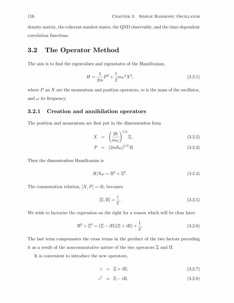
116 Chapter 3. Simple Harmonic Oscillator
density matrix, the coherent number states, the QND observable, and the time-dependent
correlation functions.
3.2 The Operator Method
The aim is to find the eigenvalues and eigenstates of the Hamiltonian,
H =1
2mP 2 +
1
2mω2X2, (3.2.1)
where P an X are the momentum and position operators, m is the mass of the oscillator,
and ω its frequency.
3.2.1 Creation and annihilation operators
The position and momentum are first put in the dimensionless form
X =
(2h
mω
)1/2
Ξ, (3.2.2)
P = (2mhω)1/2 Π. (3.2.3)
Then the dimensionless Hamiltonian is
H/hω = Π2 + Ξ2. (3.2.4)
The commutation relation, [X, P ] = ih, becomes
[Ξ, Π] =i
2. (3.2.5)
We wish to factorize the expression on the right for a reason which will be clear later:
Π2 + Ξ2 = (Ξ − iΠ)(Ξ + iΠ) +1
2. (3.2.6)
The last term compensates the cross terms in the product of the two factors preceding
it as a result of the noncommutative nature of the two operators Ξ and Π.
It is convenient to introduce the new operators,
c = Ξ + iΠ, (3.2.7)
c† = Ξ − iΠ. (3.2.8)
3.2. The Operator Method 117
From the commutation relation (3.2.5) between Ξ and Π, the commutator between the
new operators is
[c, c†] = 1. (3.2.9)
The Hamiltonian has the simple expression
H = hω(
c†c +1
2
)
. (3.2.10)
The number operator N = c†c is Hermitian and, therefore, a physical observable. From
its relation to the Hamiltonian, it is evident that N and H share common eigenstates
and their eigenvalues are simply related. We shall therefore find the eigenvalues and
eigenstates of N first.
3.2.2 The ladder theorem
If |ν〉 is an eigenstate of N with eigenvalue ν, then c|ν〉 is an eigenstate with eigenvalue
ν − 1, and c†|ν〉 is an eigenstate with eigenvalue ν + 1.
Proof: The key is the commutation relations,
[c, N ] = c , (3.2.11)[c†, N
]= −c† , (3.2.12)
which follows readily from Eq. (3.2.9). We are given
N |ν〉 = ν|ν〉. (3.2.13)
Operating on both sides with c, we obtain
cN |ν〉 = νc|ν〉. (3.2.14)
Note that we have commuted the order of c and ν on the right side since ν is a number.
The commutation relation between c and N , Eq. (3.2.11), leads to
N(c|ν〉) = (ν − 1)(c|ν〉), (3.2.15)
which means that cν is an eigenstate of N with the eigenvalue ν − 1. Q.E.D.
Similarly, it can be shown (really!) by Eq. (3.2.12) that
N(c†|ν〉) = (ν + 1)(c†|ν〉). (3.2.16)
118 Chapter 3. Simple Harmonic Oscillator
3.2.3 The ground state and zero-point motion
Since for the normalized state |ν〉
ν = 〈ν|N |ν〉 = 〈ν|c†c|ν〉 ≥ 0, (3.2.17)
where the expression ν|c†c|ν〉 is the absolute square of the length of the state vector
c|ν〉, the smallest ν must be exactly zero, otherwise ν − 1 would be a legitimate smaller
eigenvalue. For ν = 0, the same equation leads to
c|ψ0〉 = 0. (3.2.18)
The state |ν = 0〉 is the lowest energy state with energy
E0 =1
2hω. (3.2.19)
It is possible to generate the ground state wave function by expressing the state as
an expansion in the eigenstate |ξ〉 of the dimensionless position Ξ with the coefficient
ψ0(ξ) = 〈ξ|0〉, which is governed by Eq. (3.2.18),
0 = 〈ξ|c|ψ0〉 =
(
ξ +1
2
∂
∂ξ
)
ψ0(ξ), (3.2.20)
using the definition of c in Eq. (3.2.7). The normalized solution is
ψ0(ξ) =2
π
1/4
e−ξ2
,
or ψ0(x) =(
mω
πh
)1/4
e−mωx2
2h . (3.2.21)
Since the ground state energy does not enter into the spectral distribution of the
black-body radiation, there was no way for Planck to have known to include the zero
point energy in his hypothesis. The existence of motion—the zero point motion—for the
state of the lowest energy can be understood from the considerations of the uncertainty
principle, as we have seen in Chapter 1. The Gaussian wave function shows that, although
the particle is most likely to be at the origin, there is an uncertainty of position equal to√
h/2mω. Since the Fourier transform of a Gaussian is another Gaussian, the momentum
wave function has a similar distribution.

3.2. The Operator Method 119
One manifestation of the zero point motion is the fact that helium, both isotopes
He3 and He4, remains a liquid down to the lowest temperatures reached (in the milli-
degree Kelvin range), under one atmospheric pressure. In a solid made up of heavier
elements, the atoms or ions are arranged in a regular array and oscillate about the mean
equilibrium position. As the temperature approaches absolute zero, the oscillation is due
to the zero point motion. If the amplitude of the zero point oscillation (roughly speaking,
the uncertainty in position) is a small fraction of the inter-atomic distance, then the solid
remains well ordered. For a helium atom, the mass is so small that the uncertainty in
position is larger than the inter-atomic distance and the order of a solid is destroyed. It
is possible to solidify liquid helium by applying pressure at sufficiently low temperatures.
Even then the large zero point motion sets the solid helium apart from ordinary solids
with properties of a “quantum solid”.
The zero point motion of the electromagnetic field is known as the vacuum fluctua-
tions, to be considered in Chapter 14.
3.2.4 The excited states
Once we know the ground state, we can obtain all the normalized higher number or
energy eigenstates by using the ladder theorem repeatedly:
|n〉 =1√n!
(c†)n|0〉, (3.2.22)
and the corresponding energies
En =(
n +1
2
)
hω, (3.2.23)
where n is zero or a positive integer.
The ladder theorem relates two normalized adjacent number states by
c†|n〉 = γn|n + 1〉, (3.2.24)
where γn is a number to be determined by:
|γn|2〈n + 1|n + 1〉 = 〈n|cc†|n〉
= 〈n|(c†c + 1)|n〉
= n + 1. (3.2.25)
120 Chapter 3. Simple Harmonic Oscillator
In the last two steps, the commutation relation (3.2.9) and the number eigenstate prop-
erty (3.2.13) are used. Hence,
γn = (n + 1)1/2, (3.2.26)
aside from a multiplicative factor eiα with an undetermined (real) phase α which by
convention is set to zero. Thus,
c†|n〉 =√
n + 1|n + 1〉. (3.2.27)
Similarly,
c|n〉 =√
n|n − 1〉. (3.2.28)
Eq. (3.2.22) is then obtained by induction.
The energy values of the energy eigenstates, i.e., the states with definite energies, are
discrete. This is a common property of bound states. Since the potential for the harmonic
oscillator rises quadratically without limit, all the states are bound. The energy values are
separated by a regular spacing of hω. This is the essential feature of the Planck hypothesis
which is needed to derive the spectral distribution of the black-body radiation. It is very
satisfying to have this as a consequence of quantum mechanics.
3.3 Quantum Non-Demolition Observables in a Sim-ple Harmonic Oscillator
The example of a QND observable in a square well with two levels in the last chapter
is a fine academic exercise but it is not a robust system since one has to be careful not
to excite the particle out of the well. Now let us use the simple harmonic oscillator of
frequency ω as an example to find QND observables. The position and momentum of
the particle in one dimension are
X =
(h
2mω
)1/2
(c + c†), (3.3.1)
P =1
i
(mhω
2
)1/2
(c − c†), (3.3.2)
3.3. Quantum Non-Demolition Observables in a Simple Harmonic Oscillator 121
The time evolution of the operators are given in the Heisenberg representation,
c(t) = c e−iωt, (3.3.3)
c†(t) = c† eiωt. (3.3.4)
To avoid later confusion, we denote an operator in the Heisenberg representation by the
tilde over the symbol and the same operator in the Schrodinger representation by the
same symbol without the tilde. Hence, the position and momentum operators are
X(t) =
(h
2mω
)1/2
(ce−iωt + c†eiωt) = X cos ωt +P
mωsin ωt, (3.3.5)
P (t) =1
i
(mhω
2
)1/2
(ce−iωt − c†eiωt) = P cos ωt − mωX sin ωt. (3.3.6)
Note that the position and momentum operators in the Schrodinger representation are
both time independent.
Now we define in the Schrodinger representation two time dependent operators,
Qr(t) =1√2(ceiωt + c†e−iωt), (3.3.7)
Qi(t) =1
i√
2(ceiωt − c†e−iωt). (3.3.8)
They are related to the position and momentum with a trivial difference and an im-
portant difference. The trivial difference is the factor which renders the new operators
dimensionless. The important one is the time dependence which leads to their Heisenberg
representation
Qr = eiHt/hQr(t)e−iHt/h =
1√2(c + c†), (3.3.9)
Qi = eiHt/hQi(t)e−iHt/h =
1
i√
2(c − c†), (3.3.10)
which are independent of time. They are called by Walls and Milburn [4] “quadrature
phase amplitudes”. “Quadrature” means that the two phases differ by π/4, as in “the
first quarter moon is in quadrature with the sun”, or closer to our example, “the two
components of the two-phase ac current are in quadrature”. Since these phase operators
in the Heisenberg representation are independent of time, they are QND observables.
122 Chapter 3. Simple Harmonic Oscillator
The two phase operators are related to the position and momentum operators by
Qr =(
mω
h
)1/2[
X(t) cos ωt − P (t)
mωsin ωt
]
, (3.3.11)
Qi =(
mω
h
)1/2[
X(t) sin ωt +P (t)
mωcos ωt
]
. (3.3.12)
An observation useful for later use in the study of squeezed states is that the Qr − Qi
axis rotates relative to the X − P axis with angular speed −ω. A survey of experiments
on QND is given in Ref. [4].
3.4 A system of many coupled oscillators
It is straightforward to generalize the foregoing work to a coupled set of harmonic os-
cillators. When the total Hamiltonian is quadratic in the momentum variables and the
displacement from equilibrium positions of a number of particles, in classical mechan-
ics it is possible to decouple them into a set of normal modes. If each normal mode is
distinguished by a suffix j, the Hamiltonian may be written as
H =∑
j
hωj
(
c†jcj +1
2
)
. (3.4.1)
The commutation relations are
[cj, cj′ ] = 0, (3.4.2)[cj, c
†j′
]= δjj′ . (3.4.3)
In Chapter 14, it will be shown that the quantization of the electromagnetic fields can be
carried out in the same way, by determining the normal modes of the oscillations of the
electromagnetic waves and quantizing the Hamiltonian of each independent oscillator.
For a very large number of normal modes, this system is an important model for the
reservoir in the study of dissipative dynamics of an open system.
3.4.1 Vibrations of atoms in a periodic lattice
Here we study an example of coupled harmonic oscillators originating from the oscillations
of a linear chain of identical atoms with equally spaced equilibrium positions [5] moving
along the chain. To use the periodic boundary condition, we imagine the atoms to be in
3.4. A system of many coupled oscillators 123
a necklace. The atoms are labeled by the integer = 0, 1, , . . . , N − 1. Atom +N is the
same as atom . The harmonic Hamiltonian is
H =∑
[P 2
2m+
g
2(X+1 − X)
2
]
, (3.4.4)
where P is the momentum operator of the -th atom along the chain, and X its dis-
placement operator from the equilibrium position a.
For a periodic system, the translational symmetry may help in constructing the energy
eigenstates. This will be done in Chapter 8 while the treatment here is analogous to the
classical physics of small oscillations. The Heisenberg equations of motion for the coupled
oscillators are
dX
dt=
1
mP, (3.4.5)
dP
dt= g(X+1 − 2X + X−1). (3.4.6)
The equations can be decoupled by the Fourier sum,
Qk =1√N
N−1∑
=0
e−ikX,
Πk =1√N
N−1∑
=0
e−ikP. (3.4.7)
where the “lattice wave vector” k is given by
k =2πnk
N, with nk = 0, 1, . . . , N − 1. (3.4.8)
We arrive at the equations for the normal mode harmonic oscillators,
dQk
dt=
1
mΠk, (3.4.9)
dΠk
dt= −mω2
kQk, (3.4.10)
with the frequencies,
ωk = 2
√g
msin
(ka
2
)
. (3.4.11)
Each normal mode oscillator has the annihilation and creation operators given by,
Qk =
(h
2mω
)1/2
(ck + c†k), (3.4.12)
Pk = −i
(mhω
2
)1/2
(ck − c†k). (3.4.13)

124 Chapter 3. Simple Harmonic Oscillator
These relations and the inverse Fourier transforms of Eq. (3.4.7) lead directly to the
Hamiltonian (3.4.1) of N independent oscillators.
Extension to three dimensions is done first by permitting the atoms in the one dimen-
sion chain to oscillate normal to the chain. With a different (generally smaller) elastic
constant g′ for the transverse motion, there will be two transverse modes with lower fre-
quencies than the vibration along the chain which is called the longitudinal mode. Next,
the extension of the periodic structure to three dimensions can be done, for example, by
a cubic lattice of atoms. The lattice wave vector is now a vector k. For each k, there
are three normal modes in the case of a simple cubic lattice, but the direction of each
normal mode is not necessarily parallel or perpendicular to k. We may consider the index
j in the Hamiltonian (3.4.1) as the collection of indices k, ν, where the number of normal
modes per wave vector is three times the number of atoms per primitive unit cell of a
periodic lattice. For details, consult a solid state book, e.g., [5, 6]. The essential point is
the construction of the independent oscillators.
3.4.2 Second quantization - first look
We have seen how in terms of the annihilation and creation operators the Hamiltonian
can be expressed in a factorizable form, and how the Schrodinger equation is then solved
completely for the energy eigenvalues and their associated eigenstates. This method of
solution affords us a graphic interpretation of the energy eigenstates of the harmonic
oscillator. The nth level has energy nhω plus the zero point energy 12hω. Now imagine
particles each of energy hω. If the harmonic oscillator is an electromagnetic field, the
particle is called the photon. If the harmonic oscillator is from the displacement of
atoms in a solid or liquid, the particle of energy is called the phonon. Aside from the
zero point energy, the nth state of the simple harmonic oscillator may be said to be a
state containing n of these particles. The operator c† acting on the nth state yields the
(n+1)th state. c† has created a particle of energy hω and is therefore called the creation
operator. On the other hand, c acting on the nth state yields the (n − 1)th state. c
destroys a particle of energy hω and is therefore called the annihilation operator. These
operators do more than just keeping count of the number of particles; they also provide
the coherence between the two contiguous energy states since they keep the phase relation
3.5. Examples 125
between them.
For the system of N oscillators, we may think of c†j as the creation of a boson in state
j. the commutation relations are
[cj, c†j′ ] = δjj′ . (3.4.14)
In Chapter 13, the study of a system of identical particles leads to those with the com-
mutation relations like the creation and annihilation operators which are called bosons.
We could completely forget the original harmonic oscillators and their complicated wave
functions and treat the system as a bunch of particles, photons or phonons, in different
normal modes j. A general energy eigenstate of the system is
|n0, n1, . . .〉 =∏
k
[1√nk!
(c†k)nk
]
|0〉, (3.4.15)
where the quantum numbers nj are given by the number of bosons in each normal
mode j.
The first introduction of h into the commutation between the position and momentum
is called the first quantization. The quantization of the multimode wave function into a
system of Bose particles is called the second quantization.
3.5 Examples
The examples in this section are primarily for readers who have not encountered the
quantum harmonic oscillator problem previously.
3.5.1 A harmonic oscillator subject to a constant force
A simple harmonic oscillator is restricted to move in one dimension. It has mass m
and force constant mω2. It carries a charge e and is placed in a uniform static electric
field E in the line of direction of its motion. Find its energy eigenvalues and associated
eigenstates. (Hint: Do not charge into the series solution of the Schrodinger equation.
Ask yourself how you would solve the classical problem and ask if a similar procedure
could not be adopted for the corresponding quantum case.)
126 Chapter 3. Simple Harmonic Oscillator
Solution — The Hamiltonian is
H =P 2
2m+
1
2kX2 − eEX. (3.5.1)
Completing the square in X, we have
H =P 2
2m+
1
2k(X − x0)
2 − 1
2k(eE)2, (3.5.2)
where x0 = eE/k. This is a harmonic oscillator with a displaced origin at x = x0 and a
shift in energy − 12k
(eE)2. Hence, the energy eigenvalues are
En = (n +1
2)hω − (eE)2
2mω2, (3.5.3)
where n = 0, 1, 2, . . . and
ω =
√k
m. (3.5.4)
Th eigenstates are given by Eq. (3.2.22) with c† defined by X − x0 in placement of X.
3.5.2 Center of mass and relative motion
Two particles of masses m1 and m2 are confined to move in one dimension subject to an
internal conservative force between the two particles.
1. Write down the Hamiltonian for the two particles.
Solution — It is simplest to do the problem in the position representation. With
the suffices 1 and 2 denoting the respective particles, the Hamiltonian for the system
of two particles is
H =p2
1
2m1
+p2
2
2m2
+ V (x1 − x2). (3.5.5)
2. Separate the Hamiltonian into two parts: one containing the center of mass motion
only and one containing the relative motion only.
Solution — Introduce the relative coordinate
x = x1 − x2 (3.5.6)
3.5. Examples 127
and the center of mass coordinate
X =m1x1 + m2x2
m1 + m2
. (3.5.7)
To relate the relative and center-of-mass momentum operators to those of the in-
dividual particles, we use the chain rule for the differential operator
∂
∂x1
=∂x
∂x1
∂
∂x+
∂X
∂x1
∂
∂X=
∂
∂x− m1
m1 + m2
∂
∂X. (3.5.8)
Repeating the operation once more and doing the same for the second particle, we
eventually get
− h2
2m1
∂2
∂x21
− h2
2m2
∂2
∂x22
= − h2
2µ
∂2
∂x2− h2
2(m1 + m2)
∂2
∂X2, (3.5.9)
where µ is the reduced mass given by
1
µ=
1
m1
+1
m2
. (3.5.10)
Thus, the Hamiltonian is divided into two terms:
H = Hc + Hr, (3.5.11)
where the first is the center of mass motion
Hc = − h2
2(m1 + m2)
∂2
∂X2(3.5.12)
and the second is the relative motion
Hr = − h2
2µ
∂2
∂x2+ V (x). (3.5.13)
3. If the force between the two particles is simple harmonic, solve the Schrodinger
equation for the energy values and eigenstates for the system of two particles. (Do
not forget to include both relative motion and center of mass motion, or equiva-
lently, the coordinates of both particles.)
Solution — The wave function as a function of the center of mass coordinate and
the relative coordinate is now separable:
ψ(X, x) = ψc(X)ψr(x), (3.5.14)
128 Chapter 3. Simple Harmonic Oscillator
with energy
E = Ec + Er. (3.5.15)
The center of mass motion is given by the Schrodinger equation
Hcψc(X) = Ecψc(x). (3.5.16)
Therefore,
Ec =h2K2
2(m1 + m2)(3.5.17)
and
ψc(X) = eiKX . (3.5.18)
The relative motion is simple harmonic and
Ern = (n +1
2)hω, (3.5.19)
where ω =√
k/µ, and
ψrn(x) = ψn(x), (3.5.20)
the harmonic oscillator wave function.
Putting the results together, we have for the system the eigenenergy
EK,n =h2K2
2(m1 + m2)+ (n +
1
2)hω, (3.5.21)
and the associated wave function
ψK,n(X, x) = eiKXψn(x). (3.5.22)
3.5.3 Molecular vibration
Consider the vibrations of the two atoms along the line joining them in a diatomic
atom. If r denotes the distance between the two atoms, their interaction potential is
approximately given by the Morse potential
V (r) = V0
[e−2α(r−r0) − 2e−α(r−r0)
], eαr0 > 2. (3.5.23)
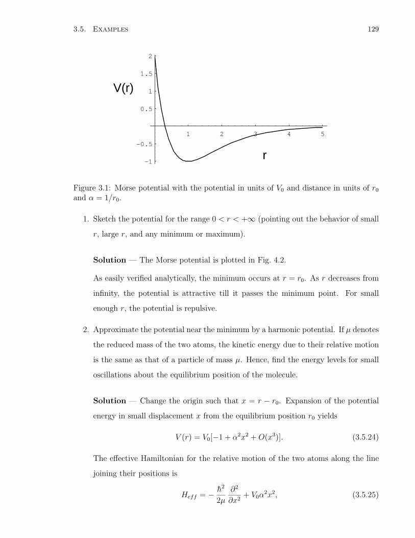
3.5. Examples 129
1 2 3 4 5
-1
-0.5
0.5
1
1.5
2
V(r)
r
Figure 3.1: Morse potential with the potential in units of V0 and distance in units of r0
and α = 1/r0.
1. Sketch the potential for the range 0 < r < +∞ (pointing out the behavior of small
r, large r, and any minimum or maximum).
Solution — The Morse potential is plotted in Fig. 4.2.
As easily verified analytically, the minimum occurs at r = r0. As r decreases from
infinity, the potential is attractive till it passes the minimum point. For small
enough r, the potential is repulsive.
2. Approximate the potential near the minimum by a harmonic potential. If µ denotes
the reduced mass of the two atoms, the kinetic energy due to their relative motion
is the same as that of a particle of mass µ. Hence, find the energy levels for small
oscillations about the equilibrium position of the molecule.
Solution — Change the origin such that x = r − r0. Expansion of the potential
energy in small displacement x from the equilibrium position r0 yields
V (r) = V0[−1 + α2x2 + O(x3)]. (3.5.24)
The effective Hamiltonian for the relative motion of the two atoms along the line
joining their positions is
Heff = − h2
2µ
∂2
∂x2+ V0α
2x2, (3.5.25)
130 Chapter 3. Simple Harmonic Oscillator
where µ is the reduced mass. The angular frequency is given by
ω =
√2V0α2
µ. (3.5.26)
The energy levels are
En = (n +1
2)hω − V0, (3.5.27)
provided that n is not so large that the quadratic approximation for V (r) breaks
down.
3. For the hydrogen molecule, V0 = 5.07 eV,
r0 = 0.74A , α = 1.88A−1
.
Compute the energy levels of the molecular vibration. (Caution: find the reduced
mass for the hydrogen molecule.)
Solution — The reduced mass is
µ = mproton/2 = 8.35 × 10⁻²⁸kg. (3.5.28)
The frequency is
ω =
[2 × 5.07eV × 1.60 × 10−19(J/eV )
8.35 × 10⁻²⁸kg
]1/2
× 1.88 × 1010/m
= 8.29 × 10¹⁴/s, (3.5.29)
and its energy is
hω = 0.54eV. (3.5.30)
The energy of the system is
En = (0.54n − 4.80)eV. (3.5.31)
4. A better approximation for the energy levels of the Morse potential are
En =(
n +1
2
)
hω −[(
n + 12
)hω
]2
4V0
− V0. (3.5.32)
3.5. Examples 131
For the hydrogen molecule, comment on the accuracy of the harmonic approxima-
tion and on its correction.
Solution — The correction ratio is
∆En
En
=(
n +1
2
)hω
V0
= 0.11(
n +1
2
)
. (3.5.33)
For the lowest level, the correction is about 10%. The corrections becomes over-
whelming at about n = 10. The tendency is to narrow the spacing between energy
levels as n increases.
3.5.4 Pendulum motion
A particle of mass m is confined to move in a vertical circle of radius R in the earth’s
gravitational field. Its position is determined by θ, the angle of its radius vector with the
downward vertical.
1. Establish the Schrodinger equation for the particle.
Solution — Treat the motion as a rigid-body rotation. The Hamiltonian is given
by
H =L2
2I+ mgR(1 − cos θ), (3.5.34)
where the moment of inertia is I = mR2 and L is the angular momentum operator
L =h
i
∂
∂θ. (3.5.35)
The time-dependent Schrodinger equation is
HΨ(θ, t) = ih∂Ψ(θ, t)
∂t. (3.5.36)
2. Show that the motion is simple harmonic if the wave function is concentrated near
θ = 0. Hence, write down the ground-state energy of the particle.
Solution — For small angular displacement θ.
1 − cos θ ≈ θ2
2, (3.5.37)
132 Chapter 3. Simple Harmonic Oscillator
and the Hamiltonian is simple harmonic
H = − h2
2mR2
∂2
∂θ2+
1
2mgRθ2, (3.5.38)
with frequency
ω =
√g
R. (3.5.39)
The ground-state energy measured from the potential energy zero is
E0 =h
2
√g
R. (3.5.40)
3. Estimate the ground-state energy in electron volts if the radius R is 1 A.
Solution —
ω =
√10m/s
10−10m≈ 3 × 10⁵/s. (3.5.41)
E0 = 10−10eV. (3.5.42)
This shows that the gravitational force is unimportant in atoms.
4. Deduce the condition on R in order that the energy in part (b) is a good approxi-
mation to the ground, given that m is about 100 times the hydrogen atom mass.
Solution — Expand the power series for the potential energy in θ to one more
term:
V (θ) = mgR(1 − cos θ) = mgR
(θ2
2− θ4
24+ O(θ6)
)
. (3.5.43)
For the harmonic approximation to be valid, the fourth order term must be smaller
than the second order:
〈θ4〉 12〈θ2〉, (3.5.44)
where the angular brackets denote the ground-state expectation value.
A sloppy way to proceed is to approximate 〈θ4〉 by 〈θ2〉2. Then the condition
Eq. (3.5.44) becomes
〈θ2〉 12. (3.5.45)
3.5. Examples 133
From the next example we see that the potential energy expectation value for the
harmonic oscillator is
1
2mgR〈θ2〉 =
1
4hω =
1
4h
√g
R. (3.5.46)
Thus, the condition for the validity of the harmonic approximation becomes
R [
h2
576m2g
]1/3
≈ 500A. (3.5.47)
A more precise treatment of the condition is to evaluate 〈θ4〉. By the operator
method, we obtain
〈(c + c†)4〉 = 5, (3.5.48)
which leads to the condition
R [
25h2
576m2g
]1/3
≈ 1500A. (3.5.49)
3.5.5 Exercises using the operator method
1. The uncertainty in momentum for the oscillator in the ground state.
Solution — The momentum expectation value for the ground state is
〈P 〉 = 〈0|P |0〉
= −i
(mhω
2
)1/2
〈0|(c − c†)|0〉, by Eq. (3.3.2)
= −i
(mhω
2
)1/2
〈0| − c†|0〉, by Eq. (3.2.18)
= i
(mhω
2
)1/2
〈0|1〉, by Eq. (3.2.27)
= 0, (3.5.50)
by the orthogonality of the eigenstates.
From Eq. (3.3.1),
P 2 = −1
2mhω(c − c†)(c − c†)
= −1
2mhω(c2 − c†c − cc† + c†2)
= −1
2mhω(c2 − 2c†c − 1 + c†2),
=1
2mhω(1 − c†2 − c2 + 2c†c). (3.5.51)
134 Chapter 3. Simple Harmonic Oscillator
To evaluate the mean value, we need
〈c†c〉 = 〈0|c†c| 0〉 = 0, by Eq. (3.2.18)
〈c2〉 = 0, for the same reason,
and 〈c†2〉 = 〈c2〉∗ = 0.
Hence, 〈P 2〉 =1
2mhω. (3.5.52)
The uncertainty is
∆p =(
1
2mhω
)1/2
. (3.5.53)
2. Ground state expectation value for the kinetic energy.
Solution —
〈T 〉 = 〈(P 2/2m)〉 =1
4hω. (3.5.54)
3. Ground state expectation value for the potential energy.
Solution —
〈V 〉 = 〈H − T 〉 =1
2hω − 1
4hω =
1
4hω. (3.5.55)
4. Uncertainty for the position of the oscillator in the ground state.
Solution — Since V = 12mω2X2,
〈X2〉 =h
2mω. (3.5.56)
Thus,
∆x =
(h
2mω
)1/2
. (3.5.57)
For the ground state, we have
∆p · ∆x =h
2. (3.5.58)
3.5. Examples 135
3.5.6 Time evolution of the oscillator state
A simple harmonic oscillator of mass m and frequence ω has a wave function at t = 0
given by
|Ψ(t = 0)〉 =1√2|0〉 + |1〉 , (3.5.59)
in terms of the two lowest energy eigenstates.
1. Find the wave function at time t.
Solution — By the procedure in Chapter 2, we obtain
|Ψ(t)〉 =1√2
|0〉e−iE0t/h + |1〉e−iE1t/h
. (3.5.60)
2. What is the probability of finding the oscillator with energy En =(n + 1
2
)hω, for
n=0,1,2,. . . ?
Solution — If the expansion of the state in terms of the energy eigenstates is
|Ψ(t)〉 =∑
n
|n〉cne−iEnt/h, (3.5.61)
then the probability of finding the particle in the state with energy En is
Pn = |cn|2. (3.5.62)
Here, the probabilities are
Pn =1
2for n = 0, 1;
Pn = 0 for n ≥ 2. (3.5.63)
3. Find the mean energy and the uncertainty.
Solution — The mean energy is
〈E〉 =∑
n
PnEn =1
2
(1
2hω +
3
2hω
)
= hω. (3.5.64)
136 Chapter 3. Simple Harmonic Oscillator
The mean square energy is
〈E2〉 =∑
n
PnE2n =
1
2
[(1
2hω
)2
+(
3
2hω
)2]
=5
4(hω)2 . (3.5.65)
The uncertainty in energy is
∆E =√
〈E2〉 − 〈E〉2 =1
2hω. (3.5.66)
This result could also be have been reached as the average is half-way between the
only two admissible energy levels.
4. Find the mean position at time t.
Solution — By definition,
〈x〉 = 〈Ψ(t)|x|Ψ(t)〉. (3.5.67)
Expanding out the energy eigenfunction series of the wave function and its complex
conjugate, we obtain
〈x〉 =1
2
[〈0|x|0〉 + eiωt〈1|x|0〉 + e−iωt〈0|x|1〉 + 〈1|x|1〉
]. (3.5.68)
Among the terms on the right, by inversion symmetry,
〈n|x|n〉 = 0, (3.5.69)
and
〈1|x|0〉 =
√h
2mω〈1|(c + c†)|0〉 =
√h
2mω. (3.5.70)
Therefore,
〈x〉 = [eiωt〈1|x|0〉
]
=
√h
2mωeiωt
=
√h
2mωcos(ωt). (3.5.71)
3.5. Examples 137
5. Find the mean momentum at time t.
Solution — By a similar argument as for the position,
〈p〉 = [eiωt〈1|p|0〉
]. (3.5.72)
The matrix element of the momentum is
〈1|p|0〉 =1
i
√mhω
2〈1|(c − c†)|0〉 = i
√mhω
2. (3.5.73)
The mean momentum at time t is
[eiωt〈1|p|0〉
]= −
√mhω
2sin(ωt). (3.5.74)
6. If at t = 0, |Ψ(t = 0)〉 = 1√2|0〉 + i|1〉, find the answers to (a)-(e). [Note: In the
normalization constant for each eigenstate, we have chosen a real number, saying
that a phase factor of eiδ is immaterial to the physics. For |Ψ(t)〉, however, the
factor of i = eiπ/2 is not an overall phase factor. (f) furnishes an example of the
importance of the relative phase of the ψ1 and ψ0 terms.]
Solution — Similar to part (a), the wave function at time t is
|Ψ(t)〉 =1√2|0〉e−iE0t/h +
i√2|1〉e−iE1t/h, (3.5.75)
The probability for finding each energy state and therefore the average energy and
uncertainty are the same as in part (a). The change in coefficient, however, changes
the mean position to
〈x〉 =1
2
[〈0|x|0〉 − ieiωt〈1|x|0〉 + ie−iωt〈0|x|1〉 + 〈1|x|1〉
]
=
−i
√h
2mωeiωt
=
√h
2mωsin(ωt). (3.5.76)
Note the change in phase of −π/2 in the oscillation of the mean position compared
with part (d).
138 Chapter 3. Simple Harmonic Oscillator
Similarly, the mean momentum is
〈p〉 = [−ieiωt〈ψ1|p|ψ0〉
]
=
√mhω
2cos(ωt). (3.5.77)
3.5.7 Matrix mechanics of the simple harmonic oscillator
We shall use the simple harmonic oscillator as an illustrative example of the matrix
mechanics in Chapter 2. In the Schrodinger representation, the evolution operator is
diagonal in the energy representation. It is, therefore, convenient to express the matrix
representation of an operator in terms of the energy eigenstates as the basis set.
From Eq. (3.2.27,3.2.28), the matrix elements of the annihilation and creation oper-
ators follow:
cmn = δm,n−1
√n , (3.5.78)
c†mn = δm,n+1(n + 1)1/2. (3.5.79)
Writing them out in matrix form, we have
c =
0 1 0 0 0 . . .
0 0√
2 0 0 . . .
0 0 0√
3 0 . . .
0 0 0 0√
4 . . .0 0 0 0 0 . . .. . . . . . . .
, (3.5.80)
and
c† =
0 0 0 0 0 . . .1 0 0 0 0 . . .
0√
2 0 0 0 . . .
0 0√
3 0 0 . . .
0 0 0√
4 0 . . .. . . . . . . .
. (3.5.81)
From the matrix forms, it is evident that c† is the Hermitian conjugate of c.
The Hamiltonian has matrix elements
Hnm = δnm
(
n +1
2
)
hω, (3.5.82)
3.5. Examples 139
i.e., diagonal:
H =1
2hω
1 0 0 0 0 . . .0 3 0 0 0 . . .0 0 5 0 0 . . .0 0 0 7 0 . . .0 0 0 0 9 . . .. . . . . . . .
. (3.5.83)
In the Heisenberg representation, the vector representation for a state of the oscillator
is frozen at a fixed time, say, at t = 0. The equation for the time development of the
operator c is
dc
dt=
i
h[H, c] = −iωc, (3.5.84)
with the help of the commutation relation (3.2.12). Hence,
c(t) = c(0) e−iωt. (3.5.85)
Similarly,
c†(t) = c†(0)eiωt. (3.5.86)
140 Chapter 3. Simple Harmonic Oscillator
3.6 Problems
1. A quantum one-dimensional harmonic oscillator has mass m, classical angular fre-
quency ω, and the bottom of the potential at the origin of the coordinate axis. At
time t = 0, it is in a state with (I) equal probability in the eigenstates with energies
(n + 12)hω and (n − 1
2)hω; (II) zero mean position; and (III) the mean momentum
in the positive axis direction.
(a) Find a state of the oscillator at time t = 0 satisfying all three conditions.
(b) Find the mean values of its position and momentum at a subsequent time t.
(c) Consider a classical oscillator with its total energy equal to the mean energy
of the above quantum oscillator. Does the classical amplitude of oscillation
agree with the largest mean value of the position of the quantum oscillator in
(b)?
2. A one-dimensional harmonic oscillator is in its ground state. Suddenly, the attrac-
tive potential on the particle is switched off so that the particle is now under no
external force. Describe what happens then by first finding the probability of the
particle flying off with momentum hk (which can be either positive or negative)
and then by a qualitative account. Contrast this with the classical harmonic oscil-
lator in its ground state and with the oscillator in a state with energy equal to the
zero-point energy.
3. Parity. The parity operator P transforms the position and momentum as
PXP† = −X, (3.6.1)
PPP† = −P. (3.6.2)
(a) Show that the parity commutes with the harmonic oscillator Hamiltonian
and, hence, that the energy eigenstates with even quantum number n are of
even parity and that the eigenstates with odd quantum number are of odd
parity. (Try to use the results of the operator method rather than the Weber
functions.)
3.6. Problems 141
(b) A particle of mass m is restricted to move in one dimension. Its potential
energy is
V (x) =1
2kx2 for x > 0 (3.6.3)
= +∞ for x < 0. (3.6.4)
i. Find the energy and wave function of its ground state. (Hint: Do not
solve the Schrodinger equation! Use the parity consideration.)
ii. Determine the uncertainties in position and momentum of the ground
state. Is the uncertainty principle obeyed?
4. Harmonic oscillator in two dimensions. A particle of mass m is confined to
move in a plane. If its position is denoted by the Cartesian coordinates (z, x), its
potential energy is given by
V (z, x) =k
2(z2 + x2), (3.6.5)
where k is the force constant.
(a) Find the energy eigenvalues and eigenstates (as state vectors) in terms of the
solutions of the one-dimensional harmonic oscillator.
(b) Find the degeneracy (i.e. the number of states) of each energy level.
(c) Show that the angular momentum operator about the y-axis, Ly = ZPx−XPz
commutes with the Hamiltonian.
(d) For the three lowest energy levels, find the eigenvalues and eigenstates of Ly
which remain energy eigenstates.
(e) Map the problem of finding the simultaneous eigenstates of H and Ly to the
angular momentum problem.
5. Correlation function of a harmonic oscillator. For the simple harmonic os-
cillator of mass m with the Hamiltonian
H = hω(
c†c +1
2
)
, (3.6.6)
where c is the annihilation operator,
142 Chapter 3. Simple Harmonic Oscillator
(a) find the time evolution of the Heisenberg operator c(t) in terms of c(0);
(b) find the evolution of 〈c†(t)c(0)〉 and 〈c†(t)c(0)〉, (i) for an energy eigenstate
and (ii) for the oscillator in thermal equilibrium at temperature T ;
(c) find the position correlation function 〈X(t)X(0)〉 for the same two cases as
above. Explain why your results are not real and how you would fix them.
6. Bose-Einstein Statistics.
Statistic mechanics tells us that, in thermodynamic equilibrium, the probability of
a system being found in a state n with energy En is proportional to exp(−En/kT )
where T is the temperature and k the Boltzmann constant. For a simple harmonic
oscillator, c†c may be regarded as the number operator measuring the number of
bosons in a state.
(a) If the system is in thermal equilibrium at temperature T , show that the ex-
pectation value 〈〈c†c〉〉 is given by the well-known Bose-Einstein distribution
function.
(b) Does the zero point energy play a role in this function? Why?
(c) Find the thermal average of eiqX (the Debye-Waller factor) where q is a wave
number and X is the position operator of a harmonic oscillator. Hint: Baker-
Hausdorff theorem for two operators with [[A, B], A] = 0 = [[A, B], B],
eA+B = e−12[A,B]eAeB. (3.6.7)
7. The coherent state represents a coherent-phase state of macroscopic number of
photons in a laser or a harmonic oscillator with a finite displacement. At time t = 0
the wave function of a simple harmonic oscillator of frequency ω is given by
|Ψ(t = 0)〉 = exp
−1
2(N + iα)
eλc+ |0〉 (3.6.8)
where |0〉 is the ground state, c+ the creation operator and λ =√
N e−iα. N is a
very large integer and α is a real phase.
3.6. Problems 143
(a) Show that
|Ψ(t = 0)〉 =∞∑
n=0
e−i(n+ 12)αf 1/2
n |n〉 (3.6.9)
where |n〉 is the nth energy eigenstate and show that the probability of finding
the system in state n is given by the Poisson distribution
fn =Nn
n!e−N . (3.6.10)
Show that the state is normalized.
(b) Prove that the coherent state is an eigenstate of c with eigenvalue λ.
(c) Find the mean value and uncertainty of the number of bosons, c+c, in this
state. Show that as N → ∞, the uncertainty is small compared with the mean
value (central limit theorem).
(d) Show that the time development of the state at time t, |Ψ(t)〉 is equivalent to
the phase α increasing as α(t) = α + ωt.
(e) Show that
〈Ψ(t)|c|Ψ(t)〉 =√
Ne−i(ωt+α). (3.6.11)
Hence, find the expectation value of the displacement of the harmonic oscilla-
tor at time t.
(f) Show that for this state
∆p · ∆x = h/2. (3.6.12)
8. Transformation to normal modes. From the transformation
X =1√N
∑
k
eik
(h
2mωk
)1/2
(ck + c†k),
P =1√N
∑
k
eik
(mhωk
2
)1/2
(−i)(ck − c†k), (3.6.13)
where k is given in Eq. (3.4.8), deduce the commutation relation [ck, c†k] and the
diagonal form of the coupled harmonic oscillator Hamiltonian, Eq. (3.4.4) in terms
of ck and c†k. Deduce also the form of ωk.
144 Chapter 3. Simple Harmonic Oscillator
9. Density of states. Phonon density of states for each polarization is defined in terms
of the frequency spectrum ωk,ν for wave vector k and polarization ν by
Dν(ω) =∑
k
δ(ω − ωk,ν), (3.6.14)
(a) Evaluate the sum for a large system at low frequency where
ωk,ν = sν |k|. (3.6.15)
(b) Hence, find the approximate expression for the zero point energy for the whole
system and the total energys if one assumes that
i. the linear dispersion holds for all k;
ii. there are one longitudinal branch and two transverse branches.
iii. the allowable k lies in a sphere in k space for N atoms.
Bibliography
[1] See any elementary text on quantum mechanics, such as R.L. Liboff, Introductory
Quantum Mechanics (Holden-Day, San Francisco, 1980).
[2] P.A.M. Dirac, Quantum Mechanics (Clarendon Press, Oxford 1958).
[3] L. Infeld and T.E. Hull, Reviews of Modern Physics 23, 21 (1951).
[4] D.F. Walls and G.J. Milburn, Quantum Optics (Springer-Verlag, Berlin,1994).
[5] J.M. Ziman, Principles of the Theory of Solids (Cambridge University Press, Cam-
bridge, 1964).
[6] A.A. Maradudin, E.M. Montroll, and G.H. Weiss, Theory of Lattice Dynamics in
the Harmonic Approximation (Academic Press, New York, 1963).
145
Chapter 4 Contents
4 Angular Momentum and Spin 1474.1 Angular Momentum and Spin . . . . . . . . . . . . . . . . . . . . . . . . 147
4.1.1 Definition of the Angular Momentum Operator . . . . . . . . . . 1474.1.2 Commutation Rules . . . . . . . . . . . . . . . . . . . . . . . . . 1484.1.3 Magnitude of the angular momentum . . . . . . . . . . . . . . . . 1494.1.4 Physical implications . . . . . . . . . . . . . . . . . . . . . . . . . 149
4.2 Angular Momentum in Spatial Representation . . . . . . . . . . . . . . . 1494.2.1 The angular momentum operators . . . . . . . . . . . . . . . . . . 1504.2.2 The magnitude squared of the angular momentum . . . . . . . . . 1514.2.3 Eigenvalues and eigenfunctions of L2 and Lz . . . . . . . . . . . . 1524.2.4 Vector model . . . . . . . . . . . . . . . . . . . . . . . . . . . . . 1544.2.5 Arbitrariness of the z direction . . . . . . . . . . . . . . . . . . . 154
4.3 Orbital Magnetic Moment . . . . . . . . . . . . . . . . . . . . . . . . . . 1604.3.1 Angular momentum and magnetic dipole moment . . . . . . . . . 1614.3.2 Magnetic dipole moment in quantum mechanics . . . . . . . . . . 161
4.4 The Stern-Gerlach Experiment . . . . . . . . . . . . . . . . . . . . . . . . 1624.4.1 Principle of the experiment . . . . . . . . . . . . . . . . . . . . . 1624.4.2 The Stern-Gerlach experiment . . . . . . . . . . . . . . . . . . . . 1624.4.3 Prediction of classical mechanics . . . . . . . . . . . . . . . . . . . 1634.4.4 Prediction of quantum mechanics . . . . . . . . . . . . . . . . . . 1634.4.5 Experimental findings . . . . . . . . . . . . . . . . . . . . . . . . 1634.4.6 Measurement of Lx . . . . . . . . . . . . . . . . . . . . . . . . . . 163
4.5 Spin of a Particle . . . . . . . . . . . . . . . . . . . . . . . . . . . . . . . 1654.5.1 Operator representation of the spin . . . . . . . . . . . . . . . . . 1654.5.2 Magnitude of spin . . . . . . . . . . . . . . . . . . . . . . . . . . . 1664.5.3 The eigen-problem of S2 and Sz . . . . . . . . . . . . . . . . . . . 1664.5.4 The raising and lowering operators . . . . . . . . . . . . . . . . . 1674.5.5 Commutation relations of S± . . . . . . . . . . . . . . . . . . . . 1674.5.6 Effects of the raising and lowering operators . . . . . . . . . . . . 1684.5.7 Theorem: β is bounded if the value of α is fixed. . . . . . . . . . . 1684.5.8 The eigenvalues . . . . . . . . . . . . . . . . . . . . . . . . . . . . 1694.5.9 Recurrence relations between eigenstates . . . . . . . . . . . . . . 1714.5.10 Matrix elements of S and S2 . . . . . . . . . . . . . . . . . . . . . 1714.5.11 Conclusion . . . . . . . . . . . . . . . . . . . . . . . . . . . . . . . 172
4.6 Electron Spin . . . . . . . . . . . . . . . . . . . . . . . . . . . . . . . . . 1734.6.1 Anomalous magnetic moment of electron spin . . . . . . . . . . . 174
i
4.6.2 Origin of the electron spin . . . . . . . . . . . . . . . . . . . . . . 1754.6.3 Electron dynamics including spin . . . . . . . . . . . . . . . . . . 1754.6.4 Spin degeneracy . . . . . . . . . . . . . . . . . . . . . . . . . . . . 1754.6.5 Hydrogen atom . . . . . . . . . . . . . . . . . . . . . . . . . . . . 176
4.7 Nucleon Spin . . . . . . . . . . . . . . . . . . . . . . . . . . . . . . . . . 1774.8 Addition of Angular Momenta . . . . . . . . . . . . . . . . . . . . . . . . 177
4.8.1 Total angular momentum . . . . . . . . . . . . . . . . . . . . . . 1774.8.2 Commutation rules . . . . . . . . . . . . . . . . . . . . . . . . . . 1784.8.3 Relationship between the two sets of eigenstates and eigenvalues . 1794.8.4 Example . . . . . . . . . . . . . . . . . . . . . . . . . . . . . . . . 1824.8.5 The vector model . . . . . . . . . . . . . . . . . . . . . . . . . . . 182
4.9 A Composite of Two Spin 12
Particles . . . . . . . . . . . . . . . . . . . . 1834.9.1 Total spin . . . . . . . . . . . . . . . . . . . . . . . . . . . . . . . 183
4.10 Examples . . . . . . . . . . . . . . . . . . . . . . . . . . . . . . . . . . . 1864.10.1 Exercise in commutation relations . . . . . . . . . . . . . . . . . . 1864.10.2 Spherical harmonics and homogeneous polynomials . . . . . . . . 1874.10.3 Rotational operator . . . . . . . . . . . . . . . . . . . . . . . . . . 1884.10.4 Stern-Gerlach experiment for spin 1/2 particles . . . . . . . . . . 1894.10.5 Zeeman splitting . . . . . . . . . . . . . . . . . . . . . . . . . . . 1914.10.6 Matrix representation of the angular momentum . . . . . . . . . . 1914.10.7 Spin-orbit interaction . . . . . . . . . . . . . . . . . . . . . . . . . 1974.10.8 Hydrogen 4f states . . . . . . . . . . . . . . . . . . . . . . . . . . 197
4.11 Problems . . . . . . . . . . . . . . . . . . . . . . . . . . . . . . . . . . . . 199
Chapter 4 List of Figures
4.1 Polar plots of the angular dependent part of the probability density . . . 1554.2 Vector diagram of the angular momentum . . . . . . . . . . . . . . . . . 1564.3 (a) Cross-section of the magnet. . . . . . . . . . . . . . . . . . . . . . . 1644.3 (b) Apparatus arrangement for the Stern-Gerlach experiment. . . . . . . 1644.4 Measuring Lx on a beam in the state Y1,1. . . . . . . . . . . . . . . . . . 1654.5 Vector model for the addition of angular momentum. . . . . . . . . . . . 184

iv
Chapter 4
Angular Momentum and Spin
Sally go round the sun,Sally go round the moon,Sally go round the chimney-potsOn a Saturday afternoon.
— Mother Goose.
4.1 Angular Momentum and Spin
Angular momentum is one property which has very interesting quantum manifestations,
which are subject to direct experimental verifications. One such experiment led to the
discovery of electron spin. A theory of the angular momentum, which does not rely
specifically on the orbital motion defining it, can be extended to describe spin which is
an intrinsic property of the particle. It is as important (and interesting) to study the
properties of spin itself as to understand the process of adding more degrees of freedom
to the motion of a particle.
4.1.1 Definition of the Angular Momentum Operator
The operator which corresponds to the physical observable, a component of the angular
momentum, is defined in the same way in terms of position and momentum as in classical
mechanics:
hL = R × P . (4.1.1)
The Cartesian components are
hLx = Y Pz − ZPy
147
148 Chapter 4. Angular Momentum and Spin
hLy = ZPx − XPz
hLz = XPy − Y Px. (4.1.2)
Since the components of position and momentum which form products in the angular
momentum are never along the same axis and therefore commute (e.g., Y Pz = PzY ),
there is no ambiguity in the quantum mechanical definition of the angular momentum and
it is not necessary to symmetrize the product of the position and momentum. Since h is
a reasonable unit of angular momentum in quantum mechanics, we follow the convention
of defining the angular momentum observable as a dimensionless operator as above.
4.1.2 Commutation Rules
In this section, we consider the commutation of the angular momentum with position,
momentum, or itself.
Define the εjk tensor as = 1 if j, k, form a cyclic permutation of x, y, z; = −1 if it
is anticyclic; = 0 otherwise. Then,
[Lj, Ak] = iεjkA, (4.1.3)
where A is R, P , or L and repeated indices are summed. We shall later give a very
general proof from the transformation properties. Here is an elementary proof:
[hLz, X] = [XPy − Y Px, X] = −Y [Px, X] = ihY. (4.1.4)
[hLz, Y ] = [XPy − Y Px, Y ] = X[Py, Y ] = −ihX. (4.1.5)
[hLz, Z] = [XPy − Y Px, Z] = 0. (4.1.6)
The other six relations can be written down by cyclically permuting the Cartesian indices.
Similarly, for momentum,
[hLz, Px] = [XPy − Y Px, Px] = [X, Px]Py = ihPy. (4.1.7)
[hLz, Py] = −ihPx. (4.1.8)
[hLz, Pz] = 0. (4.1.9)
4.2. Angular Momentum in Spatial Representation 149
The nine commutation relations of the angular momentum with itself can be suc-
cinctly summarized as
L × L = iL. (4.1.10)
In components,
[Lx, Lx] = 0 (4.1.11)
[Lx, Ly] = iLz. (4.1.12)
[Lx, Lz] = −iLy. (4.1.13)
The other six relations can be written down analogously.
4.1.3 Magnitude of the angular momentum
The square of the angular momentum is defined as
L 2 = L2x + L2
y + L2z (4.1.14)
It commutes with all three components of the angular momentum,
[Lx, L2] = 0, etc. (4.1.15)
4.1.4 Physical implications
There exist states which are simultaneous eigenstates of L 2 and only one of the three
components of the vector L, usually taken to be Lz. For these states, with wave functions
given by the spherical harmonics, L 2 and Lz can be measured simultaneously to arbitrary
accuracy. Since the components do not commute with one another, they cannot be
measured simultaneously to arbitrary accuracy.
4.2 Angular Momentum in Spatial Representation
In this section, we use the spatial representation of position and momentum operators for
the angular momentum and summarize the results of the differential equation treatment
of the eigenstate problem of L2 and Lz.
150 Chapter 4. Angular Momentum and Spin
4.2.1 The angular momentum operators
In the spatial representation, the angular momentum operator components are given in
the Cartesian axes by
Lx[x, y, z] =1
i
(
y∂
∂z− z
∂
∂y
)
Ly[x, y, z] =1
i
(
z∂
∂x− x
∂
∂z
)
Lz[x, y, z] =1
i
(
x∂
∂y− y
∂
∂x
)
. (4.2.1)
The use of the square brackets including the position coordinates indicates the fact that
the operator acts on a function of the coordinates. The functional dependence of the
operator goes beyond the position to include differential operators with respect to the
position coordinates.
The Cartesian coordinates and the spherical polars are related by
x = r sin θ cos φ,
y = r sin θ sin φ,
z = r cos θ, (4.2.2)
or the inverse relations
r = (x2 + y2 + z2)1/2,
θ = cos−1(z/r) = cos−1(z/x2 + y2 + z21/2)
φ = tan−1(y/x). (4.2.3)
The first derivatives of the spherical polars with respect to the Cartesians are
∂r∂x
= xr
= sin θ cos φ, ∂r∂y
= yr
= sin θ sin φ, ∂r∂z
= zr
= cos θ,
∂θ∂x
= 1rcos θ cos φ, ∂θ
∂y= 1
rcos θ sin φ, ∂θ
∂z= −1
rsin θ,
∂θ∂x
= −1r
sin φsin θ
, ∂φ∂y
= 1r
cos φsin θ
, ∂φ∂z
= 0.
(4.2.4)
4.2. Angular Momentum in Spatial Representation 151
The chain rules are used to convert the partial derivatives with respect to x, y, z to
the partial derivatives with respective to r, θ, φ, such as
∂
∂x=
∂r
∂x
∂
∂r+
∂θ
∂x
∂
∂θ+
∂φ
∂x
∂
∂φ, etc. (4.2.5)
Then, the Cartesian components of the angular momentum in terms of the spherical
polars are
Lx[θ, φ] = i
(
sin φ∂
∂θ+ cot θ cos φ
∂
∂φ
)
,
Ly[θ, φ] = −i
(
cos φ∂
∂θ− cot θ sin φ
∂
∂φ
)
,
Lz[θ, φ] = −i∂
∂φ. (4.2.6)
Although we are using the spherical polar coordinates, we have kept the components
of the angular momentum along the Cartesian axes, i.e., along constant directions. The
angular momentum vector is not resolved along the spherical polar coordinate unit vectors
because these vary with position and are not convenient for the purpose of integration
(which is much used in calculating expectation values, uncertainties and other matrix
elements). The functional dependence of the angular momentum operators on only the
two angular coordinates shows that it is redundant to use three position variables.
In Hamiltonian mechanics, if φ is chosen to be a generalized coordinate, then its
conjugate momentum is the angular momentum hLz. By an extension of the rule of
making the momentum conjugate of x to be the operator −ih∂/∂x, Lz would have the
expression in Eq. (4.2.6).
4.2.2 The magnitude squared of the angular momentum
From Eq. (4.2.6) one can work out the spatial representation for the angular momentum
squared,
L 2[θ, φ] = L2x + L2
y + L2z = −
[1
sin θ
∂
∂θ
(
sin θ∂
∂θ
)
+1
sin2 θ
∂2
∂φ2
]
. (4.2.7)
The θ and φ dependent part of the Laplacian in spherical polars is entirely represented
by L 2, yielding
∇2 =1
r2
∂
∂r
(
r2 ∂
∂r
)
− 1
r2L 2. (4.2.8)
152 Chapter 4. Angular Momentum and Spin
4.2.3 Eigenvalues and eigenfunctions of L2 and Lz
The commutation rules (see Sec. 4.1.2) dictate that there are no simultaneous eigenstates
of the components of the angular momentum but that it is possible to find simultaneous
eigenstates of one component and the square of the angular momentum. As a review of
the wave mechanics treatment of the angular momentum [1], we record here the simul-
taneous eigenfunctions of L 2 and Lz as spherical harmonics Ym(θ, φ):
L 2Ym = ( + 1)Ym, (4.2.9)
LzYm = mYm. (4.2.10)
The z component of the angular momentum hLz is quantized into integral multiples of h
with |m| less than or equal to . The magnitude of the angular momentum is h√
( + 1).
Note that the integer values of m are a direct consequence of the requirement that the
wave function is the wave function is unchanged by a 2π rotation about the z axis.
The spherical harmonics are determined in terms of the generalized Legendre functions
Pm :
Ym(θ, φ) = NmPm (cos θ)eimφ, (4.2.11)
with the constant
Nm =
[(2 + 1) · ( − |m|)!
4π( + |m|)!
]1/2
×
(−1)m if m > 01 if m ≤ 0
(4.2.12)
The normalization constants Nm are so chosen that the spherical harmonics form an
orthonormal set:
∫ π
0dθ
∫ 2π
0dφ sin θY ∗
′m′(θ, φ)Ym(θ, φ) = δ′δmm′ . (4.2.13)
Note that sin θdφdθ is the solid angle part of the volume element r2dr sin θdθdφ in the
spherical polars representation.
Table 4.2.3 gives the explicit expressions for the more commonly used spherical har-
monics.
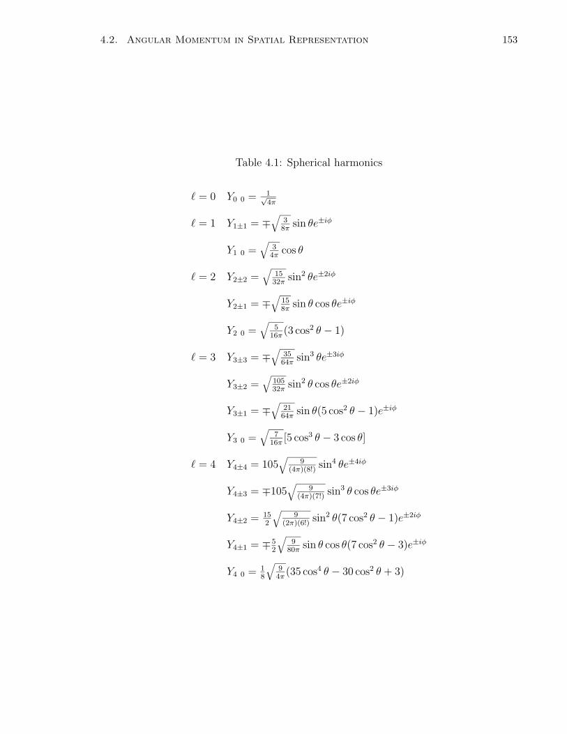
4.2. Angular Momentum in Spatial Representation 153
Table 4.1: Spherical harmonics
= 0 Y0 0 = 1√4π
= 1 Y1±1 = ∓√
38π
sin θe±iφ
Y1 0 =√
34π
cos θ
= 2 Y2±2 =√
1532π
sin2 θe±2iφ
Y2±1 = ∓√
158π
sin θ cos θe±iφ
Y2 0 =√
516π
(3 cos2 θ − 1)
= 3 Y3±3 = ∓√
3564π
sin3 θe±3iφ
Y3±2 =√
10532π
sin2 θ cos θe±2iφ
Y3±1 = ∓√
2164π
sin θ(5 cos2 θ − 1)e±iφ
Y3 0 =√
716π
[5 cos3 θ − 3 cos θ]
= 4 Y4±4 = 105√
9(4π)(8!)
sin4 θe±4iφ
Y4±3 = ∓105√
9(4π)(7!)
sin3 θ cos θe±3iφ
Y4±2 = 152
√9
(2π)(6!)sin2 θ(7 cos2 θ − 1)e±2iφ
Y4±1 = ∓52
√9
80πsin θ cos θ(7 cos2 θ − 3)e±iφ
Y4 0 = 18
√94π
(35 cos4 θ − 30 cos2 θ + 3)
154 Chapter 4. Angular Momentum and Spin
The angular dependence of the probability density is contained in the factor
Fm(θ) = |Ym(θ, φ)|2 = N2m|Pm
(cos θ)|2. (4.2.14)
It is independent of the angle φ. To get a feel for the θ dependence of the probability,
polar plots for a few Fm are given in Fig. 4.2.3. A polar plot for Fm(θ) is a plot of the
radial distance from the origin in the direction of θ equal to the function,
r = Fm(θ). (4.2.15)
These plots also give an indication of the directional dependence of the wave functions,
which is important in the consideration of chemical bonding.
4.2.4 Vector model
Since we are used to thinking in terms of classical mechanics, it is useful to represent the
quantum angular momentum in a semi-classical picture. Caution is given here that if
the picture is taken too literally it could be very misleading [2]. The angular momentum
is represented by a vector with a fixed magnitude h[( + 1)]1/2 and a fixed component
hm along the z direction, precessing about the z-axis. Figure 4.2 shows the example of
= 1. There are three vectors with magnitude h√
2, having, respectively, h, 0, −h as
the z components.
The vector has to be taken as precessing about the z-axis because the Lx and Ly
components are not well defined. Their mean values are zero. Their uncertainties are
given by
h2(〈L2x〉 + 〈L2
y〉) = h2(〈L2〉 − 〈L2z〉)
= [( + 1) − m2]h2 ≥ h2 (4.2.16)
4.2.5 Arbitrariness of the z direction
We could have chosen a component of the angular momentum along any direction. How
does one relate the eigenfunctions of L 2 and the component along this direction to the
Ym for L 2 and Lz? Suppose we rotate the Cartesian axes in some fashion and label the
new axes x′, y′, z′. The eigenfunctions of the new component Lz′ and L 2, denoted by
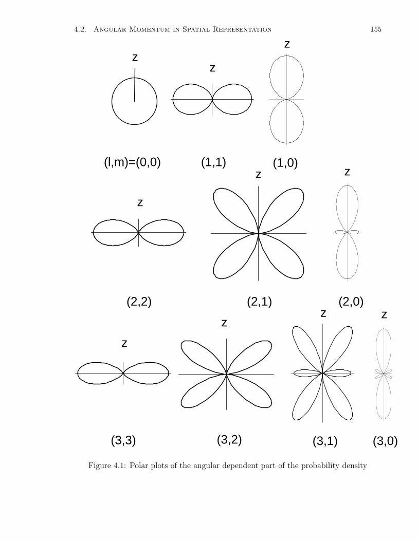
4.2. Angular Momentum in Spatial Representation 155
(l,m)=(0,0) (1,1) (1,0)
(2,2) (2,1) (2,0)
(3,3) (3,2) (3,1) (3,0)
zz
z
z
z z
z
zz z
Figure 4.1: Polar plots of the angular dependent part of the probability density
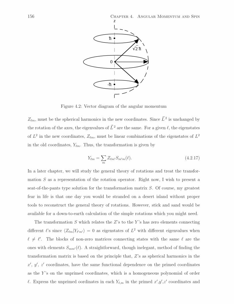
z
_√2 h
_
-h_
h_
0
156 Chapter 4. Angular Momentum and Spin
Figure 4.2: Vector diagram of the angular momentum
Zm, must be the spherical harmonics in the new coordinates. Since L 2 is unchanged by
the rotation of the axes, the eigenvalues of L 2 are the same. For a given , the eigenstates
of L2 in the new coordinates, Zm, must be linear combinations of the eigenstates of L2
in the old coordinates, Ym. Thus, the transformation is given by
Ym =∑
m
Zm′Sm′m(). (4.2.17)
In a later chapter, we will study the general theory of rotations and treat the transfor-
mation S as a representation of the rotation operator. Right now, I wish to present a
seat-of-the-pants type solution for the transformation matrix S. Of course, my greatest
fear in life is that one day you would be stranded on a desert island without proper
tools to reconstruct the general theory of rotations. However, stick and sand would be
available for a down-to-earth calculation of the simple rotations which you might need.
The transformation S which relates the Z’s to the Y ’s has zero elements connecting
different ’s since 〈Zm|Y′m′〉 = 0 as eigenstates of L2 with different eigenvalues when
= ′. The blocks of non-zero matrices connecting states with the same are the
ones with elements Smm′(). A straightforward, though inelegant, method of finding the
transformation matrix is based on the principle that, Z’s as spherical harmonics in the
x′, y′, z′ coordinates, have the same functional dependence on the primed coordinates
as the Y ’s on the unprimed coordinates, which is a homogeneous polynomial of order
. Express the unprimed oordinates in each Y,m in the primed x′,y′,z′ coordinates and
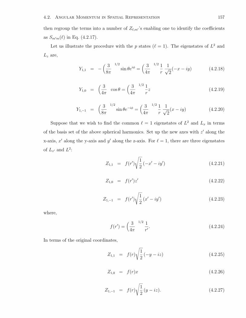
4.2. Angular Momentum in Spatial Representation 157
then regroup the terms into a number of Z,m′ ’s enabling one to identify the coefficients
as Sm′m() in Eq. (4.2.17).
Let us illustrate the procedure with the p states ( = 1). The eigenstates of L2 and
Lz are,
Y1,1 = −(
3
8π
)1/2
sin θeiφ =(
3
4π
)1/2 1
r
1√2(−x − iy) (4.2.18)
Y1,0 =(
3
4π
)
cos θ =(
3
4π
)1/2 1
rz (4.2.19)
Y1,−1 =(
3
8π
)1/2
sin θe−iφ =(
3
4π
)1/2 1
r
1√2(x − iy) (4.2.20)
Suppose that we wish to find the common = 1 eigenstates of L2 and Lx in terms
of the basis set of the above spherical harmonics. Set up the new axes with z′ along the
x-axis, x′ along the y-axis and y′ along the z-axis. For = 1, there are three eigenstates
of Lz′ and L2:
Z1,1 = f(r′)
√1
2(−x′ − iy′) (4.2.21)
Z1,0 = f(r′)z′ (4.2.22)
Z1,−1 = f(r′)
√1
2(x′ − iy′) (4.2.23)
where,
f(r′) =(
3
4π
)1/2 1
r′. (4.2.24)
In terms of the original coordinates,
Z1,1 = f(r)
√1
2(−y − iz) (4.2.25)
Z1,0 = f(r)x (4.2.26)
Z1,−1 = f(r)
√1
2(y − iz). (4.2.27)
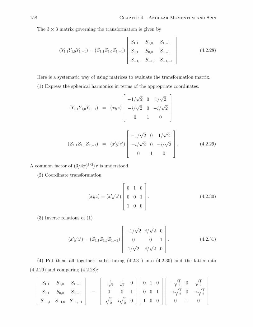
158 Chapter 4. Angular Momentum and Spin
The 3 × 3 matrix governing the transformation is given by
(Y1,1Y1,0Y1,−1) = (Z1,1Z1,0Z1,−1)
S1,1 S1,0 S1,−1
S0,1 S0,0 S0,−1
S−1,1 S−1,0 S−1,−1
(4.2.28)
Here is a systematic way of using matrices to evaluate the transformation matrix.
(1) Express the spherical harmonics in terms of the appropriate coordinates:
(Y1,1Y1,0Y1,−1) = (xyz)
−1/√
2 0 1/√
2
−i/√
2 0 −i/√
2
0 1 0
(Z1,1Z1,0Z1,−1) = (x′y′z′)
−1/√
2 0 1/√
2
−i/√
2 0 −i/√
2
0 1 0
. (4.2.29)
A common factor of (3/4π)1/2/r is understood.
(2) Coordinate transformation
(xyz) = (x′y′z′)
0 1 0
0 0 1
1 0 0
. (4.2.30)
(3) Inverse relations of (1)
(x′y′z′) = (Z1,1Z1,0Z1,−1)
−1/√
2 i/√
2 0
0 0 1
1/√
2 i/√
2 0
. (4.2.31)
(4) Put them all together: substituting (4.2.31) into (4.2.30) and the latter into
(4.2.29) and comparing (4.2.28):
S1,1 S1,0 S1,−1
S0,1 S0,0 S0,−1
S−1,1 S−1,0 S−1,−1
=
− 1√2
i√2
0
0 0 1√
12
i√
12
0
0 1 0
0 0 1
1 0 0
−√
12
0√
12
−i√
12
0 −i√
12
0 1 0
4.2. Angular Momentum in Spatial Representation 159
=
12i i
√12
i12
−√
12
0√
12
−i12
i√
12
−i12
. (4.2.32)
An alternative way, which is perhaps more physical, is to examine each state on the
right side of Eq. (4.2.28). For example,
Y1,1 = Z1,1S1,1 + Z1,0S0,1 + Z1,−1S−1,1. (4.2.33)
Substituting Eqs. (4.2.18, 4.2.25-4.2.27),
−√
1
2(x + iy) = −
√1
2(y + iz)S1,1 + xS0,1 +
√1
2(y − iz)S−1,1. (4.2.34)
Since this equality holds for all x, y and z, we can equate their coefficients on both sides:
S0,1 = −√
1
2
−S1,1 + S−1,1 = −i
−S1,1 − S−1,1 = 0. (4.2.35)
Thus,
S1,1 = i/2
S0,1 = −√
1
2
S−1,1 = −i/2. (4.2.36)
The other six elements of the transformation matrix can be found in a similar way.
Because the spherical harmonics are normalized wave functions, S must be a unitary
matrix. We verify that
|S1,1|2 + |S0,1|2 + |S−1,1|2 = 1. (4.2.37)
160 Chapter 4. Angular Momentum and Spin
Suppose that a system is prepared in the state represented by the wave function
Y1,1 with respect to a chosen z axis. Since this state is the eigenstate of L2 and Lz with
eigenvalues 2 and 1, respectively, measurement of L2 and Lz will definitely yield the same
values. If a measurement of Lx is made on this system, what will be the outcome? The
eigenstates of Lx are Z1,1, Z1,0, Z1,−1 with eigenvalues 1, 0, −1, respectively. The initial
state of the system, Y1,1, is a linear combination of the eigenstates of Lx given by Eq.
(4.2.33). The possible outcomes of the measurement of Lx are 1, 0, −1 with probabilities
|S1,1|2, |S0,1|2, |S−1,1|2, i.e. 14, 1
2, 1
4, respectively.
The mean value of Lx is
〈Lx〉 = 〈Y1,1|Lx|Y1,1〉 = |S1,1|2 · (1) + |S0,1|2 · (0) + |S−1,1|2 · (−1)
= 0. (4.2.38)
The uncertainty is given by
(∆Lx)2 = 〈L2
x〉
= |S1,1|2 · (1)2 + |S0,1|2 · (0)2 + |S−1,1|2 · (−1)2
=1
2. (4.2.39)
Hence, ∆Lx =1√2. (4.2.40)
4.3 Orbital Magnetic Moment
In Sec. 4.2.3, the z-component of the angular momentum is quantized. Loosely speaking,
the orientation of the angular momentum vector in space is quantized. This phenomenon
is known as the space quantization. How does one measure the angular momentum and
verify space quantization? Direct measurements of mechanical properties on microscopic
systems are usually very difficult. Fortunately, the electron is charged. Linear motion of
an electron creates a current. Periodic motion of an electron creates a magnetic dipole.
Electronic motion is, therefore, measured by electromagnetic means.
4.3. Orbital Magnetic Moment 161
4.3.1 Angular momentum and magnetic dipole moment
A classical derivation is given here for the relation between the angular momentum and
the magnetic dipole moment. A quantum mechanical derivation which yields the same
relation will be given later. For simplicity, consider the electron moving in a circular orbit
with speed v. (Refer to an electromagnetism text [3] for the case of a general motion.)
The angular momentum of the electron with respect to the center of the orbit is
L = mvr, (4.3.1)
where r is the radius of the orbit and m is the electron mass.
The current I is the amount of charge passing a point of the orbit per unit time:
I = (−e)v/2πr, (4.3.2)
where e denotes the charge of a proton.
The magnetic dipole moment created by the current I is
µ = Iπr2 = −evr/2 = (−e/2m)L. (4.3.3)
The magnetic dipole moment is in the same direction as the angular momentum vector.
Hence,
µ = (−e/2m)L. (4.3.4)
In an external magnetic field B, the energy of the magnetic dipole moment is
E = −µ · B. (4.3.5)
4.3.2 Magnetic dipole moment in quantum mechanics
The operator representing the magnetic moment is given by the same relation (4.3.4)
with the angular momentum. Since a component of the angular momentum is quantized
in units of h, it is convenient to write the magnetic dipole moment of the electron as
µ = −µBL, (4.3.6)
where µB = eh/2m, (4.3.7)
162 Chapter 4. Angular Momentum and Spin
is called the Bohr magneton. Thus, the z-component of the magnetic dipole moment of
the electron is quantized in units of the Bohr magneton.
In the presence of an external magnetic field B, the angular momentum of the electron
creates an additional term in the Hamiltonian,
H = −µ · B = µBL · B. (4.3.8)
Note that in a field of 1 Tesla (104 Gauss), one Bohr magneton has an energy of about
6× 10⁻⁵ eV. A field of 16 Tesla or 160 kilo-Gauss is now readily available in a laboratory
superconducting magnet.
In Eq. (4.3.7) if the electron mass is replaced by a proton mass mp and the sign of
the charge is reversed, the quantity
µN = eh/2mp, (4.3.9)
is known as the nuclear magneton, and is approximately 3×10⁻⁸ eV/T, about 2000 times
smaller than the Bohr magneton.
4.4 The Stern-Gerlach Experiment
4.4.1 Principle of the experiment
In a magnetic field B = (0, 0, B) which is non-uniform with a gradient of ∂B/∂z, the
force on a magnetic dipole is
(µ · ∇) B =
(
0, 0, µz∂B
∂z
)
. (4.4.1)
A dipole moving normal to the magnetic field will be deflected by this force. The amount
of deflection of the path of the dipole can be used to deduce the force and, therefore, the
component of the dipole moment along the field if the field gradient is known.
4.4.2 The Stern-Gerlach experiment
The cross-section of the magnet is shown in Fig. 4.3(a). The convergent magnetic line of
force creates a field gradient. The arrangement of the apparatus is shown in Fig. 4.3(b).
Neutral atoms are used in this experiment so that there is no net Lorentz force acting on
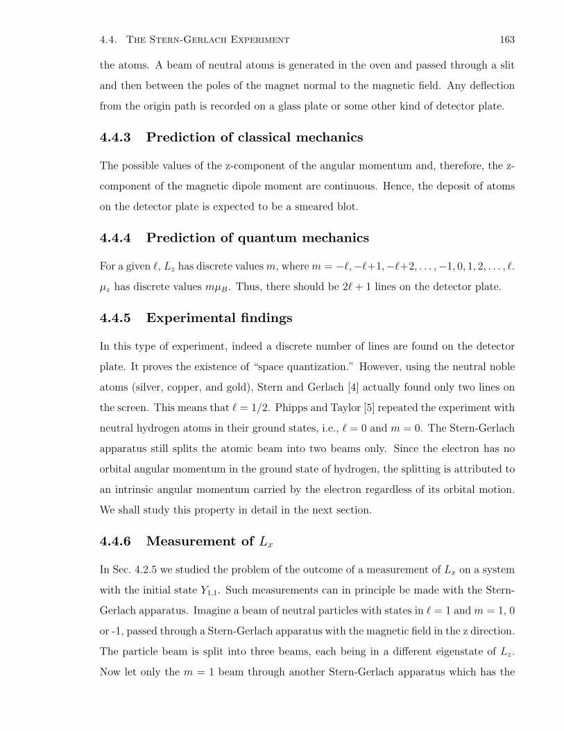
4.4. The Stern-Gerlach Experiment 163
the atoms. A beam of neutral atoms is generated in the oven and passed through a slit
and then between the poles of the magnet normal to the magnetic field. Any deflection
from the origin path is recorded on a glass plate or some other kind of detector plate.
4.4.3 Prediction of classical mechanics
The possible values of the z-component of the angular momentum and, therefore, the z-
component of the magnetic dipole moment are continuous. Hence, the deposit of atoms
on the detector plate is expected to be a smeared blot.
4.4.4 Prediction of quantum mechanics
For a given , Lz has discrete values m, where m = −,−+1,−+2, . . . ,−1, 0, 1, 2, . . . , .
µz has discrete values mµB. Thus, there should be 2 + 1 lines on the detector plate.
4.4.5 Experimental findings
In this type of experiment, indeed a discrete number of lines are found on the detector
plate. It proves the existence of “space quantization.” However, using the neutral noble
atoms (silver, copper, and gold), Stern and Gerlach [4] actually found only two lines on
the screen. This means that = 1/2. Phipps and Taylor [5] repeated the experiment with
neutral hydrogen atoms in their ground states, i.e., = 0 and m = 0. The Stern-Gerlach
apparatus still splits the atomic beam into two beams only. Since the electron has no
orbital angular momentum in the ground state of hydrogen, the splitting is attributed to
an intrinsic angular momentum carried by the electron regardless of its orbital motion.
We shall study this property in detail in the next section.
4.4.6 Measurement of Lx
In Sec. 4.2.5 we studied the problem of the outcome of a measurement of Lx on a system
with the initial state Y1,1. Such measurements can in principle be made with the Stern-
Gerlach apparatus. Imagine a beam of neutral particles with states in = 1 and m = 1, 0
or -1, passed through a Stern-Gerlach apparatus with the magnetic field in the z direction.
The particle beam is split into three beams, each being in a different eigenstate of Lz.
Now let only the m = 1 beam through another Stern-Gerlach apparatus which has the
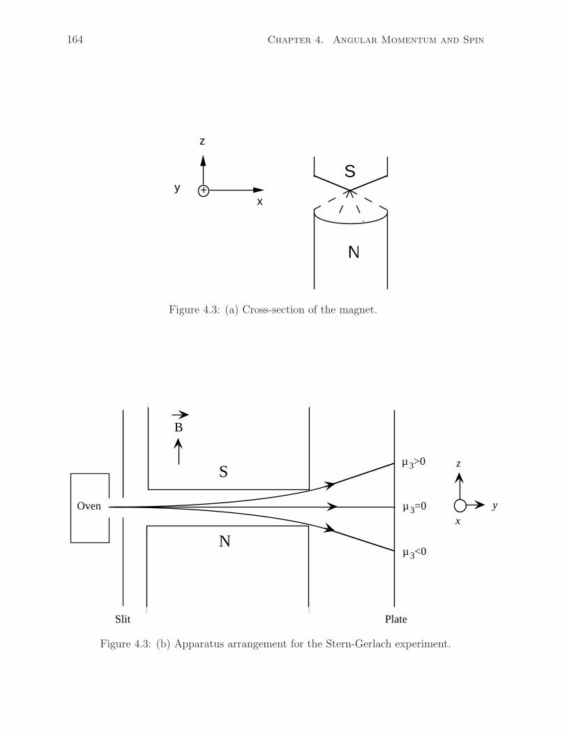
S
N
+
z
yx
Oven
Slit Plate
S
N
B
µ <03
µ =03
µ >03 z
y
x
164 Chapter 4. Angular Momentum and Spin
Figure 4.3: (a) Cross-section of the magnet.
Figure 4.3: (b) Apparatus arrangement for the Stern-Gerlach experiment.
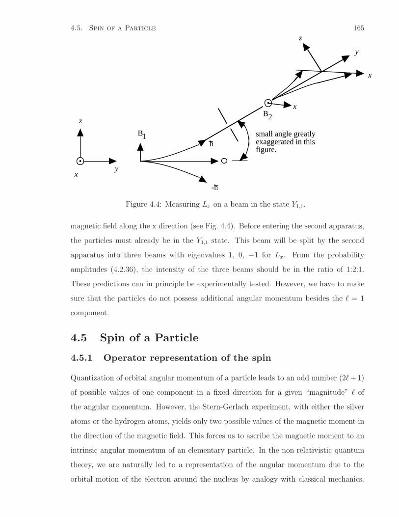
.
z
xy
x
B1
B2
-h_
h_
small angle greatlyexaggerated in this figure.
.
x
y
z4.5. Spin of a Particle 165
Figure 4.4: Measuring Lx on a beam in the state Y1,1.
magnetic field along the x direction (see Fig. 4.4). Before entering the second apparatus,
the particles must already be in the Y1,1 state. This beam will be split by the second
apparatus into three beams with eigenvalues 1, 0, −1 for Lx. From the probability
amplitudes (4.2.36), the intensity of the three beams should be in the ratio of 1:2:1.
These predictions can in principle be experimentally tested. However, we have to make
sure that the particles do not possess additional angular momentum besides the = 1
component.
4.5 Spin of a Particle
4.5.1 Operator representation of the spin
Quantization of orbital angular momentum of a particle leads to an odd number (2+1)
of possible values of one component in a fixed direction for a given “magnitude” of
the angular momentum. However, the Stern-Gerlach experiment, with either the silver
atoms or the hydrogen atoms, yields only two possible values of the magnetic moment in
the direction of the magnetic field. This forces us to ascribe the magnetic moment to an
intrinsic angular momentum of an elementary particle. In the non-relativistic quantum
theory, we are naturally led to a representation of the angular momentum due to the
orbital motion of the electron around the nucleus by analogy with classical mechanics.
166 Chapter 4. Angular Momentum and Spin
The problem now is how to construct an operator corresponding to the intrinsic angular
momentum of a particle which is independent of the position and momentum of the
particle.
Let us postulate that we may define three physical observables as the Cartesian com-
ponents of the spin vector S such that hS is the intrinsic angular momentum of a particle.
That the intrinsic angular momentum obeys the same commutation rules as the orbital
angular momentum leads to
S × S = iS. (4.5.1)
Of course, S must be Hermitian, i.e.,
S † = S. (4.5.2)
We cannot insist on the r × p representation for S; otherwise, S is not different from L
and we cannot explain the two beam result of the Stern-Gerlach experiment. Thus, the
spin S has no classical counterpart.
4.5.2 Magnitude of spin
The square of the magnitude of the spin is given by
S2 = S2x + S2
y + S2z . (4.5.3)
It follows from the commutation rules (4.5.1) that, just like the orbital angular momen-
tum,
[S, S2] = 0. (4.5.4)
4.5.3 The eigen-problem of S2 and Sz
We cannot use the spatial representation of L and solve the differential equations to
find the eigenvalues and eigenfunctions of S2 and Sz. Let us try an alternative operator
method, in analogy with the simple harmonic oscillator problem. Since the method relies
only on the commutation relations which S and L share, part of the solutions for the
general spin must be solutions of the orbital angular momentum.
4.5. Spin of a Particle 167
Since S2 and Sz commute with each other, we define their common eigenstate as |ψαβ〉with eigenvalues α and β, respectively, i.e.,
S2|ψαβ〉 = α|ψαβ〉 (4.5.5)
Sz|ψαβ〉 = β|ψαβ〉. (4.5.6)
The eigenstate |ψαβ〉 can no longer represented by a wave function of position of the
particle. We shall, however, be able to find out enough properties about these states and
their matrix representations that predictions about measurements of the spin can still be
made.
4.5.4 The raising and lowering operators
By analogy with the harmonic oscillator, we wish to factorize S2,
S2 = S2x + S2
y + S2z
= (Sx + iSy)(Sx − iSy) − Sz + S2z , (4.5.7)
where the cross terms in the product of two brackets are cancelled out by the −Sz term.
Thus, we can also define the raising and lowering operators:
S+ = Sx + iSy
S− = Sx − iSy. (4.5.8)
Since Sx and Sy are Hermitian operators, S+ and S− are not Hermitian but they are
Hermitian conjugates of each other. Then various useful expressions for S2 are:
S2 = S+S− − Sz + S2z
= S−S+ + Sz + S2z
=1
2(S+S− + S−S+) + S2
z (4.5.9)
4.5.5 Commutation relations of S±
(1) [Sz, S±] = ±S±. (4.5.10)
168 Chapter 4. Angular Momentum and Spin
Proof: [Sz, S+] = [Sz, Sx + iSy]
= [Sz, Sx] + i[Sz, Sy]
= iSy + i(−i)Sx
= (Sx + iSy).
(2) [S±, S2] = 0 (4.5.11)
(3) [S+, S−] = 2Sz. (4.5.12)
4.5.6 Effects of the raising and lowering operators
If |ψαβ〉 is an eigenstate of S2 with eigenvalue α and of Sz with eigenvalue β, then S±|ψαβ〉are eigenstates of S2 with the same eigenvalue α and eigenstates of Sz with eigenvalues
(β ± 1).
Proof: The proof that S±|ψαβ〉 are eigenstates of S2 with the same eigenvalue as |ψαβ〉 is
left as an exercise.
Sz(S+|ψαβ〉) = (SzS+)|ψαβ〉
= (S+Sz + S+)|ψαβ〉
= (β + 1)(S+|ψαβ〉). (4.5.13)
A similar proof can be constructed for S−.
Thus, S+ raises the eigenvalue of Sz by one; and S− lowers the eigenvalue of Sz by one.
Their functions are analogous to the creation and annihilation operators for a harmonic
oscillator.
4.5.7 Theorem: β is bounded if the value of α is fixed.
Since 〈ψαβ|S2|ψαβ〉 ≥ 〈ψαβ|S2z |ψαβ〉, we have,
α ≥ β2. (4.5.14)
4.5. Spin of a Particle 169
4.5.8 The eigenvalues
Since for a given α, β is bounded, there must exist a smallest value for β, which is denoted
by β1, and a largest value of β, which is denoted by β2. For a fixed α, β1 is the smallest
eigenvalue of Sz and β2 is the largest eigenvalue. Therefore,
S−|ψαβ1〉 = 0, (4.5.15)
S+|ψαβ2〉 = 0, (4.5.16)
otherwise, these two states would be eigenstates of Sz with eigenvalues (β1 − 1) and
(β2 + 1), contrary to the definitions of β1 and β2.
A useful equation is
〈S+ψαβ|S+ψαβ〉 = 〈ψαβ|(S+)†S+|ψαβ〉
= 〈ψαβ|S−S+|ψαβ〉 (4.5.17)
= 〈ψαβ|S2 − Sz − S2z |ψαβ〉 using Eq. (4.5.9),
= (α − β − β2)〈ψαβ|ψαβ〉. (4.5.18)
Since for the largest β state, raising it cannot yield another state, Eq. (4.5.16) leads to
〈S+ψαβ2|S+ψαβ2〉 = 0,
i.e., α − β2 − β22 = 0. (4.5.19)
Similarly,
〈S−ψαβ|S−ψαβ〉 = (α + β − β2)〈ψαβ|ψαβ〉. (4.5.20)
So,
α + β1 − β21 = 0. (4.5.21)
Subtracting Eq. (4.5.21) from Eq. (4.5.19),
β21 − β1 = β2
2 + β2,
or (β1 + β2)(β1 − β2 − 1) = 0. (4.5.22)
170 Chapter 4. Angular Momentum and Spin
Since β2 is greater than β1, the second bracket cannot vanish. Hence,
β2 = −β1. (4.5.23)
If the raising operator is used repeatedly on the state |ψαβ1〉, we obtain the eigenstates
of Sz
|ψαβ1〉, S+|ψαβ1〉, S2+|ψαβ1〉, . . . , Sn
+|ψαβ1〉, (4.5.24)
with eigenvalues,
β1, (β1 + 1), (β1 + 2), . . . , (β1 + n). (4.5.25)
There must exist an integer n such that after n steps the maximum value β2 is reached.
Thus,
β1 + n = β2. (4.5.26)
Using this in conjunction with Eq. (4.5.23), we obtain
β1 = −n
2, (4.5.27)
β2 =n
2, (4.5.28)
where n is zero or a positive integer. From Eq. (4.5.19),
α =n
2
(n
2+ 1
)
. (4.5.29)
To summarize, we have
S2|ψsm〉 = (s + 1)s|ψsm〉, (4.5.30)
Sz|ψsm〉 = m|ψsm〉, (4.5.31)
where, s is a half-integer or integer, i.e.
s = 0,1
2, 1,
3
2, 2,
5
2, . . . (4.5.32)
and for a given s,
m = −s, −s + 1, −s + 2, . . . , s − 1, s. (4.5.33)
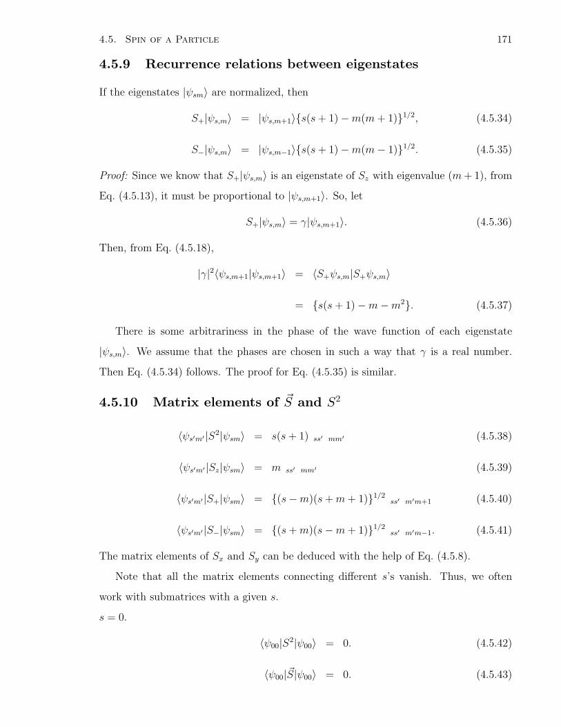
4.5. Spin of a Particle 171
4.5.9 Recurrence relations between eigenstates
If the eigenstates |ψsm〉 are normalized, then
S+|ψs,m〉 = |ψs,m+1〉s(s + 1) − m(m + 1)1/2, (4.5.34)
S−|ψs,m〉 = |ψs,m−1〉s(s + 1) − m(m − 1)1/2. (4.5.35)
Proof: Since we know that S+|ψs,m〉 is an eigenstate of Sz with eigenvalue (m + 1), from
Eq. (4.5.13), it must be proportional to |ψs,m+1〉. So, let
S+|ψs,m〉 = γ|ψs,m+1〉. (4.5.36)
Then, from Eq. (4.5.18),
|γ|2〈ψs,m+1|ψs,m+1〉 = 〈S+ψs,m|S+ψs,m〉
= s(s + 1) − m − m2. (4.5.37)
There is some arbitrariness in the phase of the wave function of each eigenstate
|ψs,m〉. We assume that the phases are chosen in such a way that γ is a real number.
Then Eq. (4.5.34) follows. The proof for Eq. (4.5.35) is similar.
4.5.10 Matrix elements of S and S2
〈ψs′m′|S2|ψsm〉 = s(s + 1)δss′δmm′ (4.5.38)
〈ψs′m′|Sz|ψsm〉 = mδss′δmm′ (4.5.39)
〈ψs′m′|S+|ψsm〉 = (s − m)(s + m + 1)1/2δss′δm′m+1 (4.5.40)
〈ψs′m′|S−|ψsm〉 = (s + m)(s − m + 1)1/2δss′δm′m−1. (4.5.41)
The matrix elements of Sx and Sy can be deduced with the help of Eq. (4.5.8).
Note that all the matrix elements connecting different s’s vanish. Thus, we often
work with submatrices with a given s.
s = 0.
〈ψ00|S2|ψ00〉 = 0. (4.5.42)
〈ψ00|S|ψ00〉 = 0. (4.5.43)
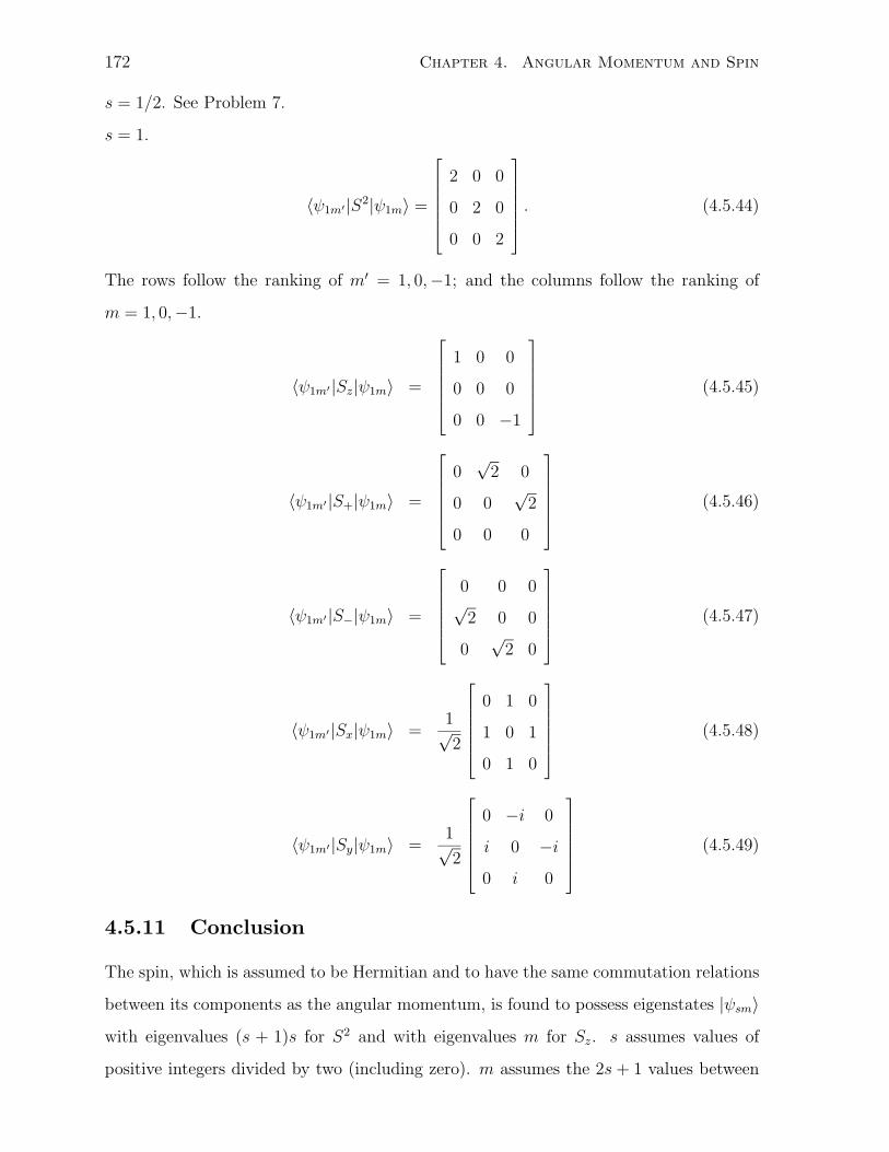
172 Chapter 4. Angular Momentum and Spin
s = 1/2. See Problem 7.
s = 1.
〈ψ1m′|S2|ψ1m〉 =
2 0 0
0 2 0
0 0 2
. (4.5.44)
The rows follow the ranking of m′ = 1, 0,−1; and the columns follow the ranking of
m = 1, 0,−1.
〈ψ1m′|Sz|ψ1m〉 =
1 0 0
0 0 0
0 0 −1
(4.5.45)
〈ψ1m′|S+|ψ1m〉 =
0√
2 0
0 0√
2
0 0 0
(4.5.46)
〈ψ1m′|S−|ψ1m〉 =
0 0 0√
2 0 0
0√
2 0
(4.5.47)
〈ψ1m′|Sx|ψ1m〉 =1√2
0 1 0
1 0 1
0 1 0
(4.5.48)
〈ψ1m′|Sy|ψ1m〉 =1√2
0 −i 0
i 0 −i
0 i 0
(4.5.49)
4.5.11 Conclusion
The spin, which is assumed to be Hermitian and to have the same commutation relations
between its components as the angular momentum, is found to possess eigenstates |ψsm〉with eigenvalues (s + 1)s for S2 and with eigenvalues m for Sz. s assumes values of
positive integers divided by two (including zero). m assumes the 2s + 1 values between
4.6. Electron Spin 173
−s and s. Thus, if s is an integer, there are an odd number of eigenstates of Sz. If s is
an integer plus a half, there are an even number of eigenstates of Sz.
If the spin is independent of position and momentum of a particle, then the eigenstate
is not expressible as a wave function of position. However, since the matrix elements of
the spin and the square of the spin are known, prediction of measurements can be made.
The orbital angular momentum, which is a vector product of position and momentum,
has the same commutation rules as the spin and ought to have eigenstates and eigenvalues
behaving the same way. However, because of its spatial dependence, a wave function of
position (or of momentum) is defined. A one-valued-ness condition is imposed on the
wave function and, consequently, the eigenstates with non-integral values of s have to be
excluded.
4.6 Electron Spin
Passing a beam of hydrogen atoms in their ground state through a Stern-Gerlach appa-
ratus results in two beams. Since the magnetic dipole moment is inversely proportional
to the mass of a particle [see Eq. (4.3.4)], the electronic dipole moment is at least a
thousand times larger than the nuclear magnetic dipole moment for the same angular
momentum. It is safe to assume that the Stern-Gerlach measurement is dominated by
the electron contribution. Since the ground state of the hydrogen atom is the = 0,
m = 0 eigenstate of the angular momentum, there is no contribution to the magnetic
dipole moment in the applied magnetic field direction from the electron orbital angular
momentum. Yet, the splitting of the beam implies the existence of a magnetic dipole
moment carried by the electron. One is forced to postulate that the electron carries an
intrinsic angular momentum independent of its orbital motion, which is called spin, to
distinguish it from the orbital angular momentum. The spin also conjures up a mental
picture of the electron being a ball of finite extent which spins about its own axis. Such a
classical picture of the electron spin can mislead us to several fruitless inferences, such as
the radius of the electron sphere (the electron is an elementary particle and is therefore
a point particle), the analogy of spin to the classical angular momentum, etc.
Furthermore, that the beam splits into two beams implies that the electron spin is in
174 Chapter 4. Angular Momentum and Spin
an s = 12
state. The electron is said to have spin “one-half.”
If the hydrogen is not in an s-state, then the magnitude of the orbital angular mo-
mentum is no longer zero. The Stern-Gerlach apparatus measures the total angular
momentum which is the sum of the orbital angular momentum and the spin of the elec-
tron.
4.6.1 Anomalous magnetic moment of electron spin
From the measurements of the deflections of the split beams, the force on the magnetic
dipole moment can be deduced. Equation (4.4.1) then yields the component of the
magnetic dipole moment along the magnetic field direction, µz, if the field gradient is
known. It turns out that
µz = ±µB. (4.6.1)
The relation between magnetic dipole moment and orbital angular momentum, Eq.
(4.3.6), has to be modified for the spin,
µ = −2µBS, (4.6.2)
since the eigenvalues of Sz are 12
and −12. The factor of two change in the relation causes
the magnetic moment of the spin to be called anomalous.
In general, when an electron possesses both spin and orbital angular momentum, its
magnetic dipole moment is
µ = −µB(gsS + g
L). (4.6.3)
g is known as the gyromagnetic ratio, or simply as the g-factor. For the electron spin,
gs = 2. (4.6.4)
For the orbital motion,
g = 1. (4.6.5)
4.6. Electron Spin 175
4.6.2 Origin of the electron spin
In the non-relativistic treatment of the electron motion by either the Schrodinger wave
mechanics or the Heisenberg matrix mechanics, the spin property of the electron has to
be grafted on. In the next chapter, we shall introduce the view that, for the double
degeneracy of the ground state found in the Stern-Gerlach experiment, the electron spin
is a natural consequence. Dirac has shown that, if the classical motion of the electron is
treated by the special relativity theory, and if the Schrodinger procedure of quantization
is followed, then the spin 12
property of the electron arises naturally in the non-relativistic
limit. This theory will be studied in Chapter 15.
4.6.3 Electron dynamics including spin
The electron properties now include not only functions of position r and momentum p,
but also of spin S. Since the spin is independent of position and momentum, it commutes
with both r and p. To specify the wave function of an electron, we require, in addition
to the three degrees of freedom given by the position r (or the momentum p), the spin
degrees of freedom. The experiments show that the electron spin is always one half.
Thus, any electron state satisfies
S2|Ψ〉 =1
2
(1
2+ 1
)
|Ψ〉 =(
3
4
)
|Ψ〉. (4.6.6)
The square of the spin operator is a constant of motion. The only additional spin variable
is sz, the eigenvalues of Sz. The other two components Sx and Sy do not commute with
Sz and cannot be used in the wave function, just as p is not used once r is chosen, or
vice versa. In general, the electron wave function is
〈r, sz|Ψ(t)〉 = Ψ(r, sz, t). (4.6.7)
4.6.4 Spin degeneracy
If the Hamiltonian of an electron is independent of its spin, then the energy eigenstates
are at least doubly degenerate.
Proof: Let Sχ be the component of S with spin 12
along some direction χ and the eigen-
176 Chapter 4. Angular Momentum and Spin
states of Sχ be denoted by |χ±〉, such that
Sχ|χ+〉 =1
2|χ+〉 (4.6.8)
Sχ|χ−〉 = −1
2|χ−〉. (4.6.9)
The states χ+ and χ− are often referred to as the spin-up state and the spin-down state.
Since the Hamiltonian is assumed to be independent of the spin variables, the energy
eigenfunctions can be found as functions of positions only as before:
Hψ(r ) = Eψ(r ). (4.6.10)
Now let the electron state including spin be
|Ψ〉 = |ψ, χσ〉, (4.6.11)
with the wave function,
Ψ(r, sz) = 〈r, sz|ψ, χσ〉 = ψ(r)χσ(sz), (4.6.12)
being a simultaneous eigenstate of H and Sχ. With the choice of σ = ±, there are two
states with energy eigenvalues E.
4.6.5 Hydrogen atom
The Hamiltonian of the hydrogen atom derived from classical mechanics (Chapter 11) is
independent of spin. There are four quantum numbers n, , m, σ specifying the energy
eigenstates, when the spin degree of freedom is included. The wave function is
ψnmσ(r, sz) = Rn(r)Ym(θ, φ)χσ(sz). (4.6.13)
The energy is unchanged:
Enmσ = −(1/n2)Ryd. (4.6.14)
The number of states with this energy is 2n2. The doubling comes from the added
possibility of spin up and down states.
4.7. Nucleon Spin 177
4.7 Nucleon Spin
Nucleon is the name given to the nuclear particles which include both proton and neutron.
The charge state of a nucleon gives the distinction between a proton and a neutron. A
nucleon has spin one-half. If S denotes the spin of a nucleon and L its orbital angular
momentum in a nucleus, then its magnetic moment is given by
µ = µN(gL + gs
S) , (4.7.1)
where g and gs are the orbital and spin g-factors. In the table below, we list the empirical
values of the g-factors:
g gs
proton 1 5.6
neutron 0 −3.8
The orbital g-factor values are as expected for the charged proton and uncharged neutron
but the expected spin g-factors are respectively 2 and 0. The explanation of the measured
values of the spin g-factors is given in terms of the internal structure of the nucleon, being
composed of three quarks.
4.8 Addition of Angular Momenta
4.8.1 Total angular momentum
An electron in an atom carries an orbital angular momentum L as well as spin S. The
total angular momentum is
J = L + S. (4.8.1)
It is important to be able to express the eigenstates of the angular momentum L2 and Lz
and the spin S2 and Sz in terms of the total angular momentum J2 and Jz (as well as of
L2 and S2) because of the conservation of the total angular momentum in the presence of
internal spin-orbit interaction. (See Sec. 4.10.7.) Let us consider the more general case
of the addition of two angular momentum operators L and S, both of which can take on
either integer or half integer values of the “magnitude” and s.
178 Chapter 4. Angular Momentum and Spin
4.8.2 Commutation rules
We start with
L × L = iL (4.8.2)
S × S = ihS (4.8.3)
[L, S] = 0. (4.8.4)
It follows that
[L, L2] = 0 (4.8.5)
[S, S2] = 0 (4.8.6)
[L, S2] = 0 (4.8.7)
[S, L2] = 0. (4.8.8)
For the sum of the angular momenta,
J × J = i J (4.8.9)
[ J, J2] = 0. (4.8.10)
Since
J2 = L2 + S2 + 2L · S, (4.8.11)
[J2, S2] = 0, (4.8.12)
and [J2, L2] = 0. (4.8.13)
Thus, we have two sets of four commutative operators:
(1) L2, Lz, S2, Sz; (4.8.14)
(2) J2, Jz, L2, S2. (4.8.15)
We may choose either set and find the simultaneous eigenstates of the four operators in
the same set.
4.8. Addition of Angular Momenta 179
4.8.3 Relationship between the two sets of eigenstates andeigenvalues
(1) The eigenstates of the first set of operators are easy to find. Let |Ym〉 be the
eigenstate of L2 and Lz with eigenvalues (+1) and m, and let |χsms〉 be the eigenstate
of S2 and Sz with eigenvalues s(s + 1) and ms. Then, the simultaneous eigenstate of all
four operators is
|ψ(msms)〉 = |Ymχsms〉. (4.8.16)
Since is not confined to the integral values, |Ym〉 here is not restricted to the spherical
harmonics. Given and s, there are (2 + 1)(2s + 1) eigenstates.
(2) Since J is an angular momentum operator satisfying the usual commutation rules,
the eigenstates of J2 and Jz can be defined as usual. In addition, however, these states
must be eigenstates of L2 and S2. Each state is characterized by four quantum numbers
j, mj, , s, such that
J2|Ψjmjs〉 = j(j + 1)|Ψjmjs〉 (4.8.17)
Jz|Ψjmjs〉 = mj|Ψjmjs〉 (4.8.18)
L2|Ψjmjs〉 = ( + 1)|Ψjmjs〉 (4.8.19)
S2|Ψjmjs〉 = s(s + 1)|Ψjmjs〉. (4.8.20)
The problem is how to relate the eigenstates |Ψjmjs〉 and their eigenvalues of the second
set of operators to those of the first set given by Eq. (4.8.16).
We note that |ψ(msms)〉 is already an eigenstate of L2 and S2. Given and s, we
only need to take linear combinations of the (2+1)(2s+1) states |ψ(msms)〉 to make
eigenstates of J2 and Jz. Now,
Jz|ψ(msms)〉 = (Lz + Sz)|ψ(msms)〉
= (m + ms)|ψ(msms)〉. (4.8.21)
This shows that |ψ(msms)〉 is already an eigenstate of Jz with eigenvalue (m+ms),
i.e. the sum of eigenvalues for Lz and Sz. It is in general not an eigenstate of J2. The
180 Chapter 4. Angular Momentum and Spin
possible values of mj are
mj = m + ms. (4.8.22)
We shall now find, given and s, what are the values of j. The largest value of mj is
(mj)max = + s. (4.8.23)
Since mj ranges from −j to j, the largest possible value of j is
jmax = + s. (4.8.24)
Since there is only one such state |ψ(ss)〉, this state must be an eigenstate of J2 and
Jz, i.e. |Ψ+s +s s〉. This statement can easily be verified directly by operating
J2 = J−J+ + Jz + J2z (4.8.25)
on the state |ψ(ss)〉, since J+ annihilates the state and each Jz produces a factor of
+ s.
The second largest value of mj is
mj = + s − 1. (4.8.26)
There are two such |ψ(msms)〉 states with
m = − 1 and ms = s (4.8.27)
and m = , ms = s − 1. (4.8.28)
Two suitable linear combinations of these two states will be eigenstates |Ψjmjs〉, with
j = + s, mj = + s − 1, (4.8.29)
j = + s − 1, mj = + s − 1. (4.8.30)
The former is a state of j = + s with the second largest mj. The latter is a state of
j = + s − 1 with the largest mj.
In the same way, the next value of mj is + s− 2 with three possible combinations of
m and ms. They yield three states with the same mj but three different j values: + s,
+ s − 1, + s − 2.

4.8. Addition of Angular Momenta 181
We can keep going in this manner. The smallest value of j, which must be positive, is
| − s| because the total number of possible product states |ψ(msms)〉 for given and
s is exhausted:
+s∑
j=|−s|(2j + 1) = ( + s − | − s| + 1)( + s + | − s| + 1)
= (2 + 1)(2s + 1). (4.8.31)
This yields just the right number of combinations for the unitary transformation:
|Ψjmjs〉 =∑
m
∑
ms
|Ymχsms〉〈Ym
χsms |Ψjmjs〉, (4.8.32)
where,
〈Ymχsms |Ψjmjs〉 = C
jmj
m,sms=
j s
mj m ms
(4.8.33)
denoted by the Clebsch-Gordan coefficient, or the 3j symbol. We shall delay the study
of the general theory for these coefficients but for now work out only a couple of specific
examples in the next section.
There is an alternative way to obtain the largest value of j (say, jmax) and the smallest
value of j (say, jmin). The total number of states with and s is on the one hand
jmax∑
j=jmin
(2j + 1) =1
2(2jmax + 1 + 2jmin + 1)(jmax − jmin + 1)
= (jmax + jmin + 1)(jmax − jmin + 1), (4.8.34)
and on the other hand (2 + 1)(2s + 1). If > s, the solution is
jmax + jmin = 2,
jmax − jmin = 2s, (4.8.35)
yielding
jmax = + s,
jmin = − s. (4.8.36)
182 Chapter 4. Angular Momentum and Spin
4.8.4 Example
Let us illustrate the above procedure with an example. Let = 1 and s = 12. For
instance, we wish to find the total angular momentum of the electron (carrying a spin 12)
in a p state of the hydrogen atom. There are 6 eigenstates of L2, Lz, S2 and Sz with m
and ms chosen from
m = 1, 0,−1
ms =1
2,−1
2.
From Eq. (4.8.22), the possible values of mj are
32, 1
2, −1
2, −3
2.
(1, 1
2
) (1,−1
2
) (0,−1
2
) (−1,−1
2
)
(0, 1
2
) (−1, 1
2
)
Under each value of mj is a column of combinations of (m, ms). Thus, the possible
values of j and mj are
j =3
2, mj =
3
2,1
2,−1
2,−3
2;
and j =1
2, mj =
1
2,−1
2.
They correspond to exactly 6 states. The (m, ms) =(1, 1
2
)state is the only one with
mj = 32
and, thus, it must be an eigenstate of J2 with j = 32. The two states (m, ms) =
(1,−1
2
)and
(0, 1
2
)have mj = 1
2and suitable linear combinations can be made from them
to yield an eigenstate of J2 with j = 32
and one with j = 12.
4.8.5 The vector model
In Section 4.2.4, a semi-classical picture of the angular momentum is described in which
it is represented by a vector precessing about the z-axis with a fixed z component equal
to the eigenvalue of the z component of the angular momentum operator. Now, all
three angular momenta, L, S and their sum J can be represented by three precessing
vectors. The vector J is given in terms of L and S by the usual vector addition rule.
For the example above, the three possible orientations of the vector L are illustrated in
4.9. A Composite of Two Spin 12 Particles 183
Fig. 4.5(a), and the two possible states of the vector S are illustrated in Fig. 4.5(b). The
z-component of the vector J must be the sum of the z components of L and S. Figures
4.5(c) and (d) show the possible combinations of vector additions of the precessing vectors
L and S.
4.9 A Composite of Two Spin 12 Particles
Besides the electron, there are other particles with spin 12, e.g. the neutron and the
proton. Consider a system of two spin 12
particles, either identical, such as two protons
in the hydrogen molecule, or dissimilar, such as the electron and proton in the hydrogen
atom or the neutron and proton in the deuteron. We shall work out this example of two
spins not only for the eigenvalues but also eigenstates of the total spin J2 and Jz.
Using the notations of the last section, let L and S be the spin operators of the two
particles. Then
=1
2, and s =
1
2. (4.9.1)
For simplicity, denote the eigenstates of Lz with eigenvalues ±12
by |φ±〉 and those of Sz
by |χ±〉. The four eigenstates of L2, Lz, S2, and Sz are |φ+χ+〉, |φ+χ−〉, |φ−χ+〉, |φ−χ−〉.
4.9.1 Total spin
The possible values of j, mj are
j = 0, mj = 0;
and j = 1, mj = 1, 0,−1. (4.9.2)
Denote the eigenstates of J2 and Jz by |Ψjmj〉, with the quantum numbers and s
understood to be a half.
From Eq. (4.8.21), |φ+χ+〉 is an eigenstate of Jz with eigenvalue
mj = m + ms = 1. (4.9.3)
Since there is only one such state, the j = 1 mj = 1 state must be
|Ψ1,1〉 = |φ+χ+〉. (4.9.4)
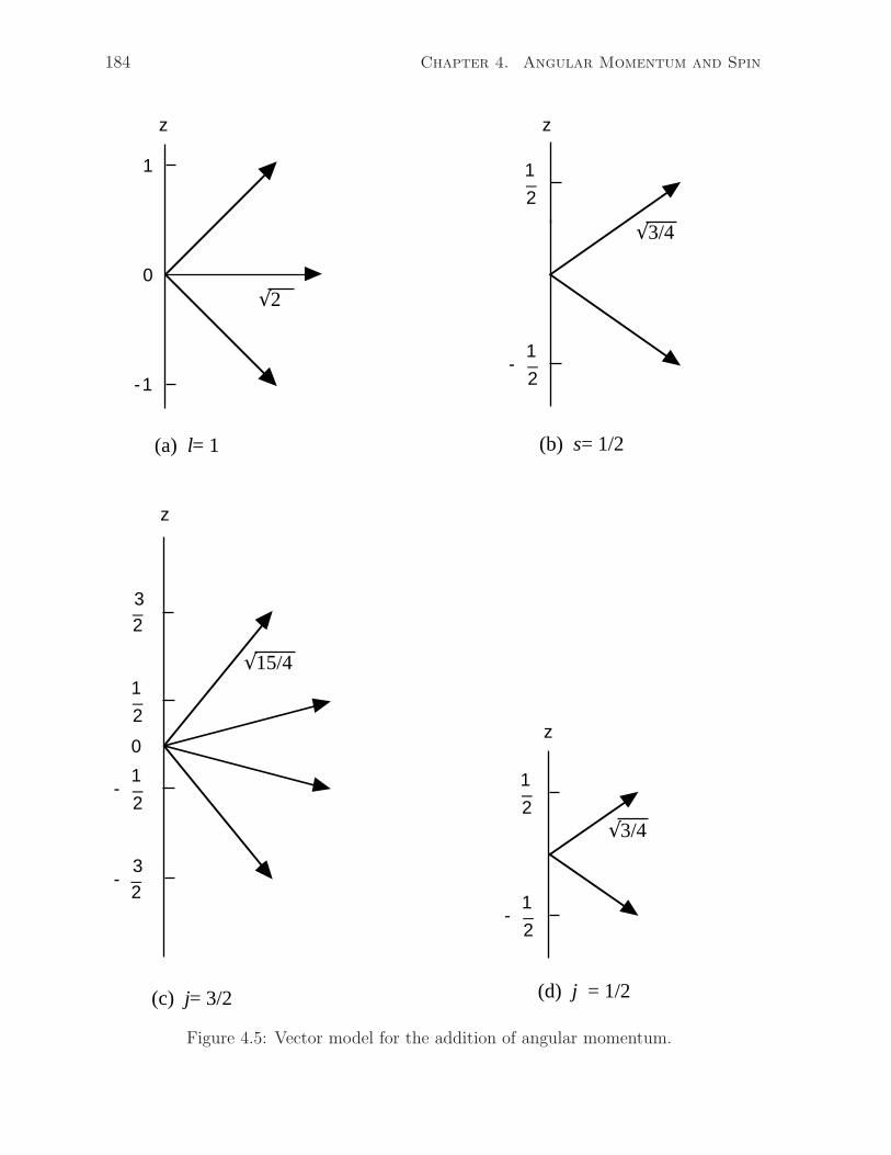
√15/4
z
3_2
3_2
-
0
1_2
1_2
-
√3/4
z
1_2
1_2
-
(c) j= 3/2 (d) j = 1/2
√3/4
√2
z z
1
0
-1
(a) l= 1 (b) s= 1/2
1_2
1_2
-
184 Chapter 4. Angular Momentum and Spin
Figure 4.5: Vector model for the addition of angular momentum.
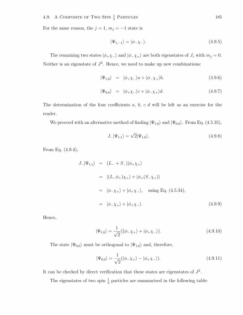
4.9. A Composite of Two Spin 12 Particles 185
For the same reason, the j = 1, mj = −1 state is
|Ψ1,−1〉 = |φ−χ−〉. (4.9.5)
The remaining two states |φ+χ−〉 and |φ−χ+〉 are both eigenstates of Jz with mj = 0.
Neither is an eigenstate of J2. Hence, we need to make up new combinations:
|Ψ1,0〉 = |φ+χ−〉a + |φ−χ+〉b, (4.9.6)
|Ψ0,0〉 = |φ+χ−〉c + |φ−χ+〉d. (4.9.7)
The determination of the four coefficients a, b, c d will be left as an exercise for the
reader.
We proceed with an alternative method of finding |Ψ1,0〉 and |Ψ0,0〉. From Eq. (4.5.35),
J−|Ψ1,1〉 =√
2|Ψ1,0〉. (4.9.8)
From Eq. (4.9.4),
J−|Ψ1,1〉 = (L− + S−)|φ+χ+〉
= |(L−φ+)χ+〉 + |φ+(S−χ+)〉
= |φ−χ+〉 + |φ+χ−〉, using Eq. (4.5.34),
= |φ−χ+〉 + |φ+χ−〉. (4.9.9)
Hence,
|Ψ1,0〉 =1√2(‖φ−χ+〉 + |φ+χ−〉). (4.9.10)
The state |Ψ0,0〉 must be orthogonal to |Ψ1,0〉 and, therefore,
|Ψ0,0〉 =1√2(|φ−χ+〉 − |φ+χ−〉). (4.9.11)
It can be checked by direct verification that these states are eigenstates of J2.
The eigenstates of two spin 12
particles are summarized in the following table:
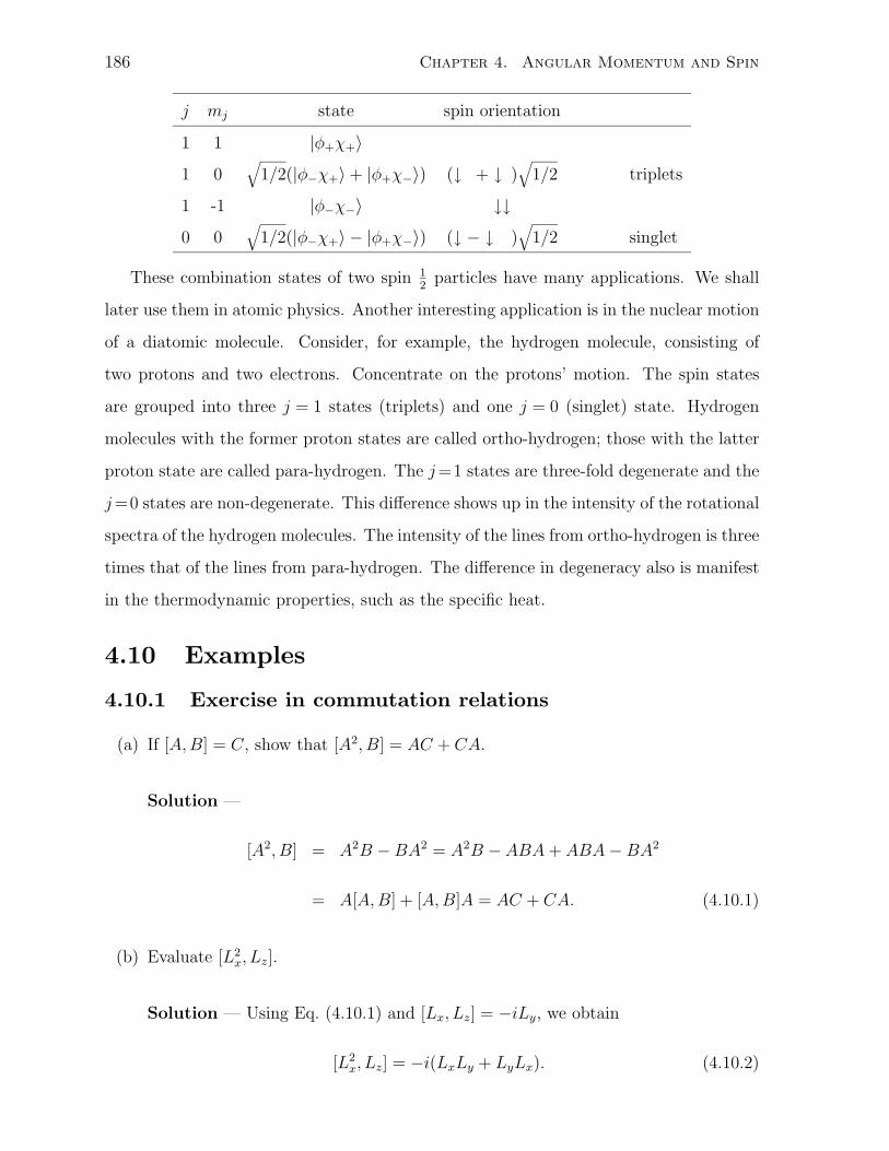
186 Chapter 4. Angular Momentum and Spin
j mj state spin orientation
1 1 |φ+χ+〉 ↑↑1 0
√1/2(|φ−χ+〉 + |φ+χ−〉) (↑↓ + ↓↑)
√1/2 triplets
1 -1 |φ−χ−〉 ↓↓0 0
√1/2(|φ−χ+〉 − |φ+χ−〉) (↑↓ − ↓↑)
√1/2 singlet
These combination states of two spin 12
particles have many applications. We shall
later use them in atomic physics. Another interesting application is in the nuclear motion
of a diatomic molecule. Consider, for example, the hydrogen molecule, consisting of
two protons and two electrons. Concentrate on the protons’ motion. The spin states
are grouped into three j = 1 states (triplets) and one j = 0 (singlet) state. Hydrogen
molecules with the former proton states are called ortho-hydrogen; those with the latter
proton state are called para-hydrogen. The j =1 states are three-fold degenerate and the
j =0 states are non-degenerate. This difference shows up in the intensity of the rotational
spectra of the hydrogen molecules. The intensity of the lines from ortho-hydrogen is three
times that of the lines from para-hydrogen. The difference in degeneracy also is manifest
in the thermodynamic properties, such as the specific heat.
4.10 Examples
4.10.1 Exercise in commutation relations
(a) If [A, B] = C, show that [A2, B] = AC + CA.
Solution —
[A2, B] = A2B − BA2 = A2B − ABA + ABA − BA2
= A[A, B] + [A, B]A = AC + CA. (4.10.1)
(b) Evaluate [L2x, Lz].
Solution — Using Eq. (4.10.1) and [Lx, Lz] = −iLy, we obtain
[L2x, Lz] = −i(LxLy + LyLx). (4.10.2)
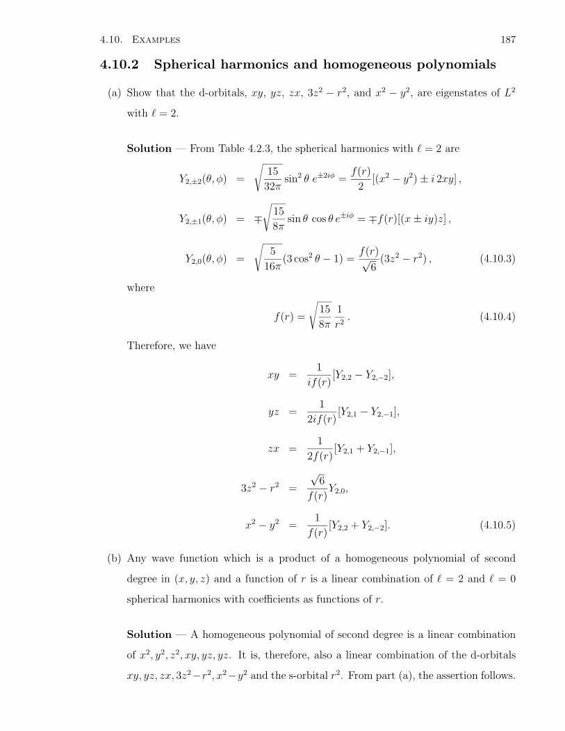
4.10. Examples 187
4.10.2 Spherical harmonics and homogeneous polynomials
(a) Show that the d-orbitals, xy, yz, zx, 3z2 − r2, and x2 − y2, are eigenstates of L2
with = 2.
Solution — From Table 4.2.3, the spherical harmonics with = 2 are
Y2,±2(θ, φ) =
√15
32πsin2 θ e±2iφ =
f(r)
2[(x2 − y2) ± i 2xy] ,
Y2,±1(θ, φ) = ∓√
15
8πsin θ cos θ e±iφ = ∓f(r)[(x ± iy)z] ,
Y2,0(θ, φ) =
√5
16π(3 cos2 θ − 1) =
f(r)√6
(3z2 − r2) , (4.10.3)
where
f(r) =
√15
8π
1
r2. (4.10.4)
Therefore, we have
xy =1
if(r)[Y2,2 − Y2,−2],
yz =1
2if(r)[Y2,1 − Y2,−1],
zx =1
2f(r)[Y2,1 + Y2,−1],
3z2 − r2 =
√6
f(r)Y2,0,
x2 − y2 =1
f(r)[Y2,2 + Y2,−2]. (4.10.5)
(b) Any wave function which is a product of a homogeneous polynomial of second
degree in (x, y, z) and a function of r is a linear combination of = 2 and = 0
spherical harmonics with coefficients as functions of r.
Solution — A homogeneous polynomial of second degree is a linear combination
of x2, y2, z2, xy, yz, yz. It is, therefore, also a linear combination of the d-orbitals
xy, yz, zx, 3z2−r2, x2−y2 and the s-orbital r2. From part (a), the assertion follows.
188 Chapter 4. Angular Momentum and Spin
4.10.3 Rotational operator
(a) Show that a rotational operator, which rotates any wave function rigidly through
an angle α about the z-axis, can be express as
R(α, z) = e−iαLz . (4.10.6)
Solution — See Problem 12 in Chapter 1. The effect of the operator on a wave
function is
R(α, z)ψ(r, θ, φ) = ψ(r, θ, φ − α)
=∞∑
n=0
1
n!
(
−α∂
∂φ
)n
ψ(r, θ, φ)
= e−α ∂∂φ ψ(r, θ, φ)
= e−iαLzψ(r, θ, φ). (4.10.7)
(b) Is R(α, z) a Hermitian operator?
Solution — No, its Hermitian conjugate is
R†(α, z) = eiαLz , (4.10.8)
which is not equal to R(α, z) except in the trivial case of α = 0.
(c) Find the transformation matrix which connects the = 1 spherical harmonics to
the eigenstates of = 1 of Lx′ where x′ is obtained by rotating the x-axis through
an angle α about the z-axis.
Solution — By using the rotation operator, we obtain the new eigenstates
Z1,1 = R(α, z)Y1,1 = Y1,1e−iα,
Z1,0 = R(α, z)Y1,0 = Y1,0,
Z1,−1 = R(α, z)Y1,−1 = Y1,−1eiα. (4.10.9)
4.10. Examples 189
The transformation S, which is given by
Y1,m =1∑
m′=−1
Z1,m′Sm′,m, (4.10.10)
is, therefore, a diagonal matrix
S =
eiα 0 0
0 1 0
0 0 e−iα
. (4.10.11)
(d) What is the most general expression for a rotation operator?
Solution — A rotation may be expressed as through an angle α about an axis in
the direction of the unit vector n. Thus, from part (a), it can be represented by
R(α,n) = e−iαn·L. (4.10.12)
4.10.4 Stern-Gerlach experiment for spin 1/2 particles
Platt [7] complained that most textbook treatments of the Stern-Gerlach experiment
were based on semiclassical quantum mechanics. Indeed, the account in this chapter is
also based on the semiclassical orbital argument. He gave a quantum treatment. Here is
a simplified version of his paper for the spin 1/2 particles in a Stern-Gerlach apparatus.
(a) Wave function representation of the spin 1/2 particle in three dimensions.
Solution — If |Ψ〉 represents the state of the particle, and |r,±〉 represents the
eigenstate of position at r and spin state in the z direction ±1/2, then
Ψ(r,±) = 〈r,±|Ψ〉 (4.10.13)
is the two-component wave function.
(b) The time-dependent Schrodinger equation.
Solution — The time-dependent Schrodinger equation is given by
ih∂
∂t|Ψ〉 = H|Ψ〉 (4.10.14)
190 Chapter 4. Angular Momentum and Spin
with the Hamiltonian given by
H =P 2
2m− gµB
S · B, (4.10.15)
in a non-uniform magnetic field B = (0, 0, βz). Applying 〈r,±| to Eq. (4.10.14)
yields the two-component Schrodinger equation for the wave functions:
ih∂Ψ(r,±)
∂t= − h2
2m∇2Ψ(r,±) ∓ 1
2gµBβzΨ(r,±). (4.10.16)
(c) The particle paths and their interpretation.
Solution — If we apply the Ehrenfest theorem separately to each spin component
of the wave function, we obtain the equations of motion for the separate expectation
values 〈r〉± = 〈Ψ(±)|r|Ψ(±)〉
d〈r〉±dt
=〈p〉±m
,
d〈p〉±dt
= ±1
2gµBβzk, (4.10.17)
where k is the unit vector in the z direction.
While the equations no doubt give us two mathematical paths, one for each spin
state, the interpretation for the prediction of experimental outcome requires care.
Suppose that spatially each particle is prepared as a wave packet. Remember that
if the state wave function is normalized at a given time, then
〈Ψ(+)|Ψ(+)〉 + 〈Ψ(−)|Ψ(−)〉 = 1. (4.10.18)
This reminds us that 〈Ψ(±)|Ψ(±)〉 for the wave packet are measures of the proba-
bilities of the particle being in either path. Thus, if we set up the detector screen
as in Fig. 4.3, the two intersects of the paths with the screen give us the positions
for the spin up and down states and their intensities give us the probabilities in
these spin states. A single particle can end up in either point, with its associated
probability.
4.10. Examples 191
4.10.5 Zeeman splitting
A hydrogen atom in its ground state is placed in a uniform magnetic field of 200 Tesla.
Calculate the energy difference of the two-spin states to two significant figures in elec-
tron volts and the frequency of the electromagnetic wave which would cause resonance
absorption between the two levels.
Solution — The Hamiltonian for the spin in magnetic field B along the z direction
is
H = − gsµB SzB. (4.10.19)
The energy difference for the two states with Sz given by ±12
is
∆E = − gsµB B(−1
2− 1
2
)
= gsµBB
= 2 × 5.79 × 10−5 eV/T × 200 T
= 0.023 eV. (4.10.20)
We have used the g-factor of the electron spin to be 2 and the value of the Bohr magneton
from the table of Fundamental Physical Constants. Note that it agrees with the energy
on the last but one line of the table.
Thus, from the same line of the table, the corresponding frequency for the electro-
magnetic wave is
ν = 0.028 THz/T × 200 T
= 5.6 THz. (4.10.21)
4.10.6 Matrix representation of the angular momentum
(a) Evaluate the matrix elements of L for the = 2 states.
Solution — In the basis set of the common eigenstates of Lz and L2, Y,m, all the
matrix elements of L and L2 connecting states of different ’s vanish. Thus, we can
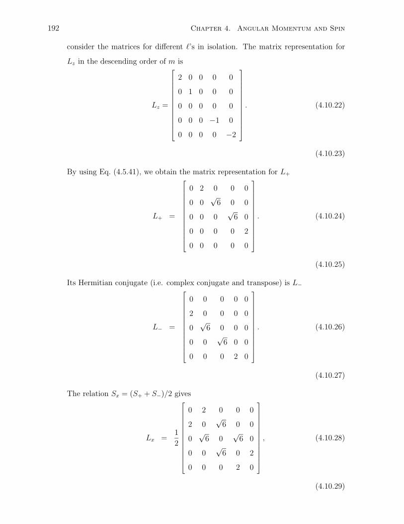
192 Chapter 4. Angular Momentum and Spin
consider the matrices for different ’s in isolation. The matrix representation for
Lz in the descending order of m is
Lz =
2 0 0 0 0
0 1 0 0 0
0 0 0 0 0
0 0 0 −1 0
0 0 0 0 −2
. (4.10.22)
(4.10.23)
By using Eq. (4.5.41), we obtain the matrix representation for L+
L+ =
0 2 0 0 0
0 0√
6 0 0
0 0 0√
6 0
0 0 0 0 2
0 0 0 0 0
. (4.10.24)
(4.10.25)
Its Hermitian conjugate (i.e. complex conjugate and transpose) is L−
L− =
0 0 0 0 0
2 0 0 0 0
0√
6 0 0 0
0 0√
6 0 0
0 0 0 2 0
. (4.10.26)
(4.10.27)
The relation Sx = (S+ + S−)/2 gives
Lx =1
2
0 2 0 0 0
2 0√
6 0 0
0√
6 0√
6 0
0 0√
6 0 2
0 0 0 2 0
, (4.10.28)
(4.10.29)
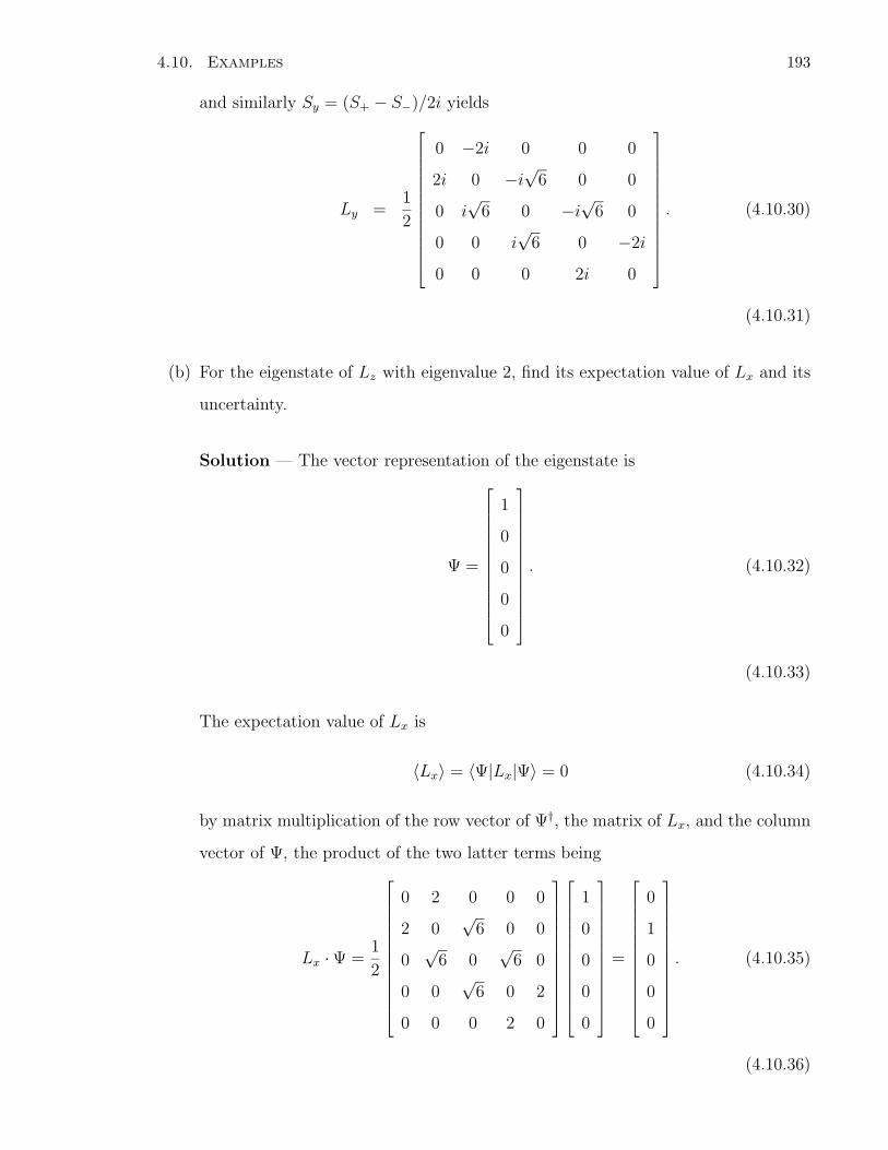
4.10. Examples 193
and similarly Sy = (S+ − S−)/2i yields
Ly =1
2
0 −2i 0 0 0
2i 0 −i√
6 0 0
0 i√
6 0 −i√
6 0
0 0 i√
6 0 −2i
0 0 0 2i 0
. (4.10.30)
(4.10.31)
(b) For the eigenstate of Lz with eigenvalue 2, find its expectation value of Lx and its
uncertainty.
Solution — The vector representation of the eigenstate is
Ψ =
1
0
0
0
0
. (4.10.32)
(4.10.33)
The expectation value of Lx is
〈Lx〉 = 〈Ψ|Lx|Ψ〉 = 0 (4.10.34)
by matrix multiplication of the row vector of Ψ†, the matrix of Lx, and the column
vector of Ψ, the product of the two latter terms being
Lx · Ψ =1
2
0 2 0 0 0
2 0√
6 0 0
0√
6 0√
6 0
0 0√
6 0 2
0 0 0 2 0
1
0
0
0
0
=
0
1
0
0
0
. (4.10.35)
(4.10.36)
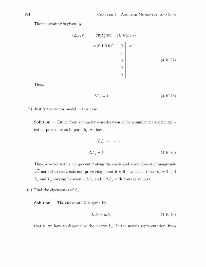
194 Chapter 4. Angular Momentum and Spin
The uncertainty is given by
(∆Lx)2 = 〈Ψ|L2
x|Ψ〉 = 〈LxΨ|LxΨ〉
= [0 1 0 0 0]
0
1
0
0
0
= 1.
(4.10.37)
Thus,
∆Lx = 1. (4.10.38)
(c) Justify the vector model in this case.
Solution — Either from symmetry consideration or by a similar matrix multipli-
cation procedure as in part (b), we have
〈Ly〉 = = 0,
∆Ly = 1 (4.10.39)
Thus, a vector with a component 2 along the z-axis and a component of magnitude√
2 normal to the z-axis and precessing about it will have at all times Lz = 2 and
Lx and Ly varying between ±∆Lx and ±∆Ly with average values 0.
(d) Find the eigenstates of Lx.
Solution — The eigenstate Φ is given by
LxΦ = mΦ, (4.10.40)
that is, we have to diagonalize the matrix Lx. In the matrix representation, from
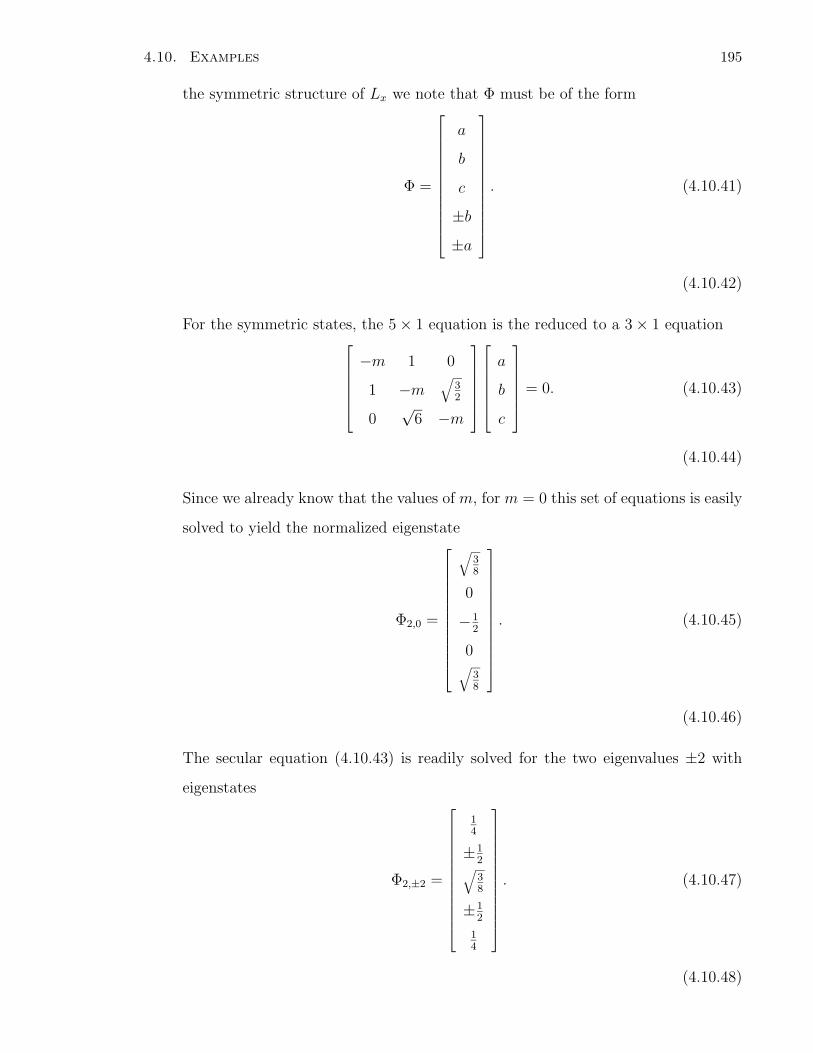
4.10. Examples 195
the symmetric structure of Lx we note that Φ must be of the form
Φ =
a
b
c
±b
±a
. (4.10.41)
(4.10.42)
For the symmetric states, the 5 × 1 equation is the reduced to a 3 × 1 equation
−m 1 0
1 −m√
32
0√
6 −m
a
b
c
= 0. (4.10.43)
(4.10.44)
Since we already know that the values of m, for m = 0 this set of equations is easily
solved to yield the normalized eigenstate
Φ2,0 =
√38
0
−12
0√
38
. (4.10.45)
(4.10.46)
The secular equation (4.10.43) is readily solved for the two eigenvalues ±2 with
eigenstates
Φ2,±2 =
14
±12
√38
±12
14
. (4.10.47)
(4.10.48)
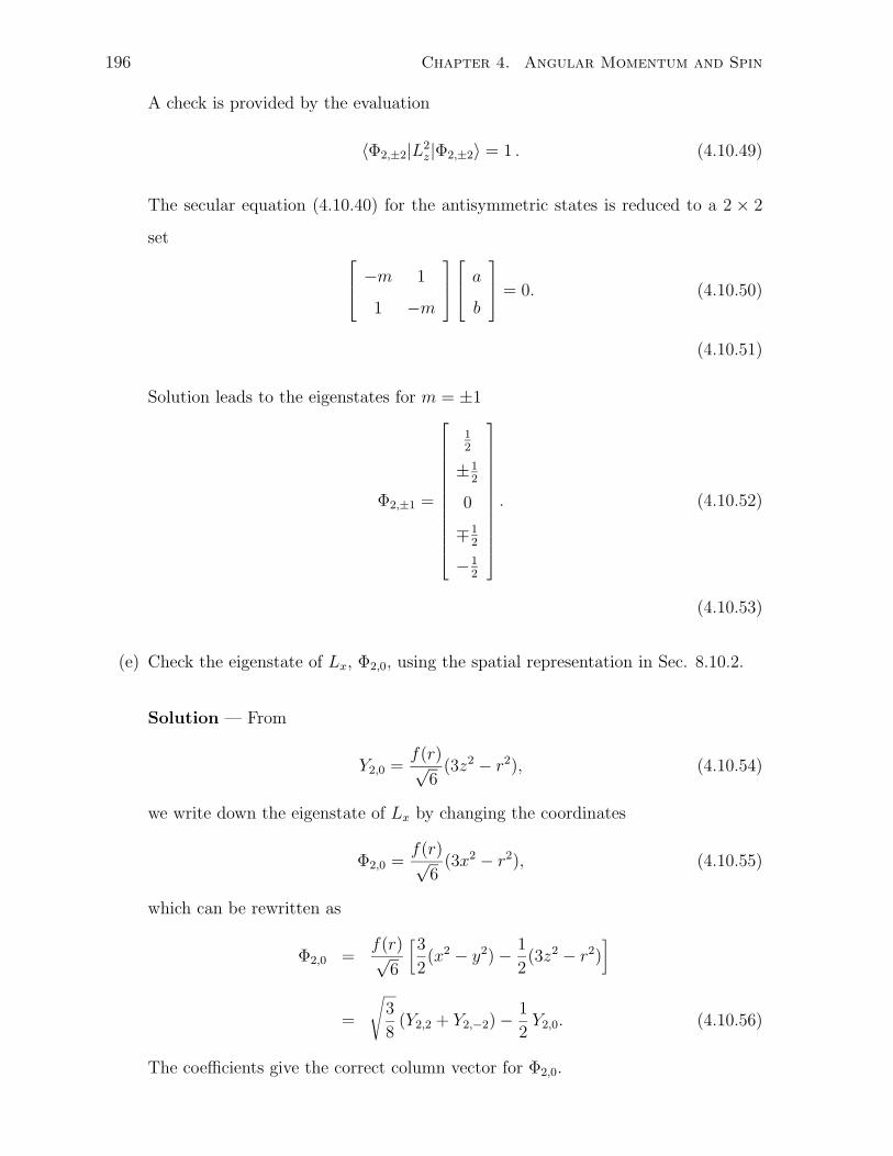
196 Chapter 4. Angular Momentum and Spin
A check is provided by the evaluation
〈Φ2,±2|L2z|Φ2,±2〉 = 1 . (4.10.49)
The secular equation (4.10.40) for the antisymmetric states is reduced to a 2 × 2
set
−m 1
1 −m
a
b
= 0. (4.10.50)
(4.10.51)
Solution leads to the eigenstates for m = ±1
Φ2,±1 =
12
±12
0
∓12
−12
. (4.10.52)
(4.10.53)
(e) Check the eigenstate of Lx, Φ2,0, using the spatial representation in Sec. 8.10.2.
Solution — From
Y2,0 =f(r)√
6(3z2 − r2), (4.10.54)
we write down the eigenstate of Lx by changing the coordinates
Φ2,0 =f(r)√
6(3x2 − r2), (4.10.55)
which can be rewritten as
Φ2,0 =f(r)√
6
[3
2(x2 − y2) − 1
2(3z2 − r2)
]
=
√3
8(Y2,2 + Y2,−2) −
1
2Y2,0. (4.10.56)
The coefficients give the correct column vector for Φ2,0.
4.10. Examples 197
4.10.7 Spin-orbit interaction
We give here a reason why sometimes the eigenstates of J2, Jz, L2, and S2 are preferred to
those of L2, Lz, S2, and Sz. Later, we shall establish the interaction between the magnetic
dipole moment due to the orbital motion and the spin magnetic dipole moment. Here we
argue that the interaction between L and S must have spherical symmetry since there
is no reason for a special direction. The invariants are L2, S2 and L · S. The first two
depend only on the individual properties. The interaction must involve the last one. The
Hamiltonian is of the form
Hso = 2ζ L · S, (4.10.57)
where ζ is independent of the angular and spin coordinates. The spin-orbit interaction
may be rewritten as
Hso = ζ (J2 − L2 − S2). (4.10.58)
It is evident then that an eigenstate of J2, Jz, L2, and S2 is also an eigenstate of Hso,
with the eigenvalue ζ[j(j + 1) − ( + 1) − s(s + 1)]. That eigenvalue of the interaction
has a 2j + 1-fold degeneracy.
4.10.8 Hydrogen 4f states
(a) If the electron of a hydrogen atom is in the 4f state, list by appropriate quan-
tum numbers the eigenstates of the z-components of the electron orbital angular
momentum and spin. By using the vector model or otherwise, list by appropriate
quantum numbers the eigenstates of J2 and Jz of the total angular momentum
(spin plus orbital).
Solution — Let L denote the orbital angular momentum and S the spin. For the
4f level, = 3. Thus, the additional quantum numbers in this level are given by
(m, ms), with m in integers ranging from −3 to 3 and ms = ±1/2. There are in
total 14 states.
The total angular momentum, J = L + S, has quantum numbers for J2 and Jz
denoted by (j, mj). The possible values of j range from | − s| in unit increments
198 Chapter 4. Angular Momentum and Spin
to + s. Thus,
j = 3 ± 1
2=
5
2or
7
2. (4.10.59)
For j = 52,
mj = −5
2, −3
2,−1
2,
1
2,
3
2,
5
2; (4.10.60)
for j = 72,
mj = −7
2, . . . ,
7
2. (4.10.61)
There are again 14 states.
(b) Find the component of the magnetic dipole moment along the z-direction in units
of the Bohr magneton of the eigenstate of J2 and Jz with the largest eigenvalues
for a 4f electron.
Solution — The largest eigenvalues of J2 and Jz are (j, mj) = (72, 7
2). The associ-
ated state is
Ψ 72, 72
= Y3,3ψ 12, 12, (4.10.62)
where the terms on the right side are the eigenstates of the orbital angular momen-
tum and spin respectively.
The z component of the magnetic dipole moment is given by
µz = −µe(Lz + 2Sz). (4.10.63)
Acting on the (72, 7
2) state yields
µzΨ 72, 72
= −µB(Lz + 2Sz)Y3,3ψ 12, 12
= −µB[(LzY3,3)ψ 12, 12
+ Y3,3(2Szψ 12, 12)]
= −µB[(3Y3,3)ψ 12, 12
+ Y3,3(ψ 12, 12)]
= −4µBΨ 72, 72. (4.10.64)
This shows that the state is also an eigenstate of µz with eigenvalue −4µB.
4.11. Problems 199
4.11 Problems
1. From the definition of the orbital angular momentum, deduce the commutation
relations:
L × L = iL,
[L, L2] = 0.
2. Let the three components of K be Hermitian operators with the commutation
relations:
[Ky, Kz] = iKx, [Kz, Kx] = iKy, [Kx, Ky] = −iKz. (4.11.1)
No, the minus sign in the last equation is not a typo. (For a more detailed discussion
of these generators of the SO(2,1) group, see [6]).
(a) Establish the following relations:
[Kz, K±] = ±K± for K± = Kx ± iKy; (4.11.2)
[K−, K+] = 2Kz; (4.11.3)
if M = K2z − K2
x − K2y , then M = K2
z − Kz − K+K−; (4.11.4)
[M, K
]= 0. (4.11.5)
(b) Hence use the raising and lower operators on the common eigenstates of Kz
and M to find the possible values of their eigenvalues.
3. The unnormalized wave function of a particle at some instant of time is
Ψ(r) = (x + y + z)F (x2 + y2 + z2),
where F is a given function. Find all the possible outcomes and their associated
probabilities that a measurement of the square of the magnitude of the angular
momentum L2 and the z component Lz will yield. Is the state an eigenstate of
n · L, where n is a unit vector to be determined?
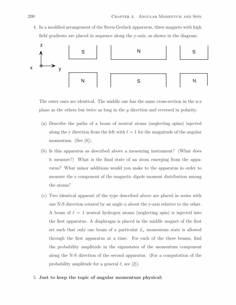
x y
zS
N
N
NS
S
200 Chapter 4. Angular Momentum and Spin
4. In a modified arrangement of the Stern-Gerlach apparatus, three magnets with high
field gradients are placed in sequence along the y-axis, as shown in the diagram.
The outer ones are identical. The middle one has the same cross-section in the x-z
plane as the others but twice as long in the y direction and reversed in polarity.
(a) Describe the paths of a beam of neutral atoms (neglecting spins) injected
along the y direction from the left with = 1 for the magnitude of the angular
momentum. (See [8]).
(b) Is this apparatus as described above a measuring instrument? (What does
it measure?) What is the final state of an atom emerging from the appa-
ratus? What minor additions would you make to the apparatus in order to
measure the z component of the magnetic dipole moment distribution among
the atoms?
(c) Two identical apparati of the type described above are placed in series with
one N-S direction rotated by an angle α about the y-axis relative to the other.
A beam of = 1 neutral hydrogen atoms (neglecting spin) is injected into
the first apparatus. A diaphragm is placed in the middle magnet of the first
set such that only one beam of a particular Lz momentum state is allowed
through the first apparatus at a time. For each of the three beams, find
the probability amplitude in the eigenstates of the momentum component
along the N-S direction of the second apparatus. (For a computation of the
probability amplitude for a general , see [2]).
5. Just to keep the topic of angular momentum physical:
4.11. Problems 201
(a) Compute the field gradient of a meter-long Stern-Gerlach magnet necessary to
produce a 1 mm separation at the end of the magnet between the components
of a beam of neutral atoms with no spin and with orbital angular momentum
= 1 incident with kinetic energy of 1000 K.
(b) The ground state of 57Fe (a favorite nucleus for the Mossbauer experiment)
has a spin 1/2 ground state. Nuclear magnetic resonance (more about that in
the next chapter) gives a change of the resonance frequency of 1.38 MHz at
an additional magnetic field of 1 T. Deduce the g-factor for 57Fe.
6. If S denotes the spin angular momentum and S± = Sx ± iSy, show that
[S±, S2] = 0,
and hence, show that if ψαβ is an eigenstate of S2 and Sz, then S±ψαβ are also
eigenstates of S2 with the same eigenvalue as ψαβ.
7. Exercises in angular momentum.
(a) Evaluate the matrix elements 〈ψsm|S|ψsm′〉 of all three components of the
angular momentum for s =1, 12, and 3
2.
(b) For the eigenstate of Lz with eigenvalue 1 and of L2 with = 1, find its
expectation value of Lx and its uncertainty.
(c) Find the eigenstates of Lx with = 1 from its matrix representation.
(d) Check the eigenstate of Lx with eigenvalue 1, using the spatial representation
in Eq. (4.2.29).
8. For the orbital angular momentum L, find the expressions for the raising and
lowering operators L± = Lx ± iLy in terms of the spherical polar coordinates. Use
the properties of these raising and lowering operators to find the = 2 normalized
eigenfunctions for Lz and L2, given one of them:
Y2,0 =
√5
16π(3 cos2 θ − 1) ∝ P2(cos θ).
202 Chapter 4. Angular Momentum and Spin
9. If the electron of a hydrogen atom is in the 3d state, list by appropriate quan-
tum numbers the eigenstates of the z-components of the electron orbital angular
momentum and spin. By using angular momentum addition, list by appropriate
quantum numbers the eigenstates of J2 and Jz of the total angular momentum
(spin plus orbital).
Find the component of the magnetic dipole moment along the z-direction in units
of the Bohr magnetons of the eigenstate of J2 and Jz with the largest eigenvalues
for a 3d electron.
10. In a system of two spin one-half particles, |φ±〉 and |χ±〉 denote the spin-up and
spin-down states of the two particles respectively.
(a) Show that |φ+χ−〉 and |φ−χ+〉 are eigenstates of the z-component of the total
spin Jz but not of the square of the total momentum J2.
(b) Find the 2× 2 matrix of J2 with respect to the two states |φ+χ−〉 and |φ−χ+〉and diagonalize it to find the eigenvalues and eigenstates of J2.
(c) Why is it not necessary in (b) to consider the matrix elements of J2 connecting
the state |φ+χ−〉 or the state |φ−χ+〉 to either |φ+χ+〉 or |φ−χ−〉?
11. A deuteron (2H) is composed of a proton and a neutron. Let us think of the state
of the deuteron as due to the two spin one-half constituent particles moving around
each other with a central potential. Let the total angular momentum be
I = Sp + Sn + L,
being the sum of the proton spin, neutron spin and the orbital angular momentum.
(a) The measured total angular momentum of the deuteron is i = 1. Show that
the four possible states are:
i. Spz and Snz parallel with = 0,
ii. Spz and Snz antiparallel with = 1,
iii. Spz and Snz parallel with = 1,
4.11. Problems 203
iv. Spz and Snz parallel or antiparallel with = 2.
(b) The spatial parity of deuteron is determined by studying nuclear reactions
involving deuterons to be even. Show that this eliminates the = 1 states.
(c) The experimentally measured magnetic dipole moment of the deuteron is
0.8574µN . By calculating the maximum magnetic dipole moment for the = 0
and the maximum magnetic dipole moment = 2 states, show that the state
of deuteron is = 0.
12. Consider angular momentum addition J = L + S. |, s; j, m〉 ≡ |j, m〉 is an eigen-
state respectively of L2, S2, J2, and Jz; while |, s; m, ms〉 ≡ |m, ms) denotes an
eigenstate respectively of L2, S2, Lz, and Sz.
(a) Find the eigenstate |j = +s, m = +s〉 in terms of |m, ms). By means of the
lowering operator J− = L− + S− find the eigenstate |j = + s, m = + s− 1〉in terms of |m, ms).
(b) Hence, find the eigenstate |j = + s − 1, m = + s − 1〉 in terms of |m, ms).
(c) Explain briefly how to use the lowering operator J− to construct in principle
the eigenstate |j, m〉 in terms of |m, ms).
13. Find the eigenvalues and eigenstates of J2 and Jz of the total angular momentum
J = L + S for = 1 and s = 12
in terms of the eigenstates of L2, S2, Lz and Sz.
This problem has a number of applications, e.g. the “holes” in the valence band of
a III-V semiconductor [9].

204 Chapter 4. Angular Momentum and Spin
Bibliography
[1] See, for example, R.L. Liboff, Introductory Quantum Mechanics (Holden-Day, San
Francisco, 1980).
[2] K. Schonhammer, Am. J. Phys. 68, 49 (2000).
[3] For example, J.R. Reitz, F.J. Milford, and R.W. Christy, Foundations of electro-
magnetic theory, 4th edition (Addison-Wesley, Reading, Mass., 1993).
[4] O. Stern, Zeits. f. Physik 7, 249 (1921); W. Gerlach and O. Stern, Ann. d. Physik
74, 673 (1924).
[5] T. E. Phipps and J. B. Taylor, Phys. Rev. 29, 309 (1927).
[6] K.T. Hecht, Quantum Mechanics (Springer-Verlag, new York 2000).
[7] D.E. Platt, Am. J. Phys. 60, 306 (1992).
[8] R.P. Feynman, R.B. Leighton, and M. Sands, The Feynman Lectures on Physics,
Vol. III, (Addison-Wesley, Reading, Mass., 1965) Chapter 5.
[9] P.Y. Yu and M. Cardona, Fundamentals of Semiconductors (Springer-Verlag, Berlin,
1996).
205
Chapter 5 Contents
5 Two-State Systems 2075.1 The general two-state system . . . . . . . . . . . . . . . . . . . . . . . . 207
5.1.1 States and observables . . . . . . . . . . . . . . . . . . . . . . . . 2075.1.2 The spin one-half language . . . . . . . . . . . . . . . . . . . . . . 2085.1.3 Properties of the Pauli matrices . . . . . . . . . . . . . . . . . . . 2095.1.4 Mapping the two-state system to the spin one-half particle . . . . 2095.1.5 Spin-1/2 Hamiltonian in a magnetic field – redux . . . . . . . . . 2115.1.6 Examples of two-state systems . . . . . . . . . . . . . . . . . . . . 212
5.2 Energy Eigenstates of Spin 12
Particle . . . . . . . . . . . . . . . . . . . . 2145.2.1 Magnetic field splitting . . . . . . . . . . . . . . . . . . . . . . . . 2145.2.2 Magnetic field in a general direction . . . . . . . . . . . . . . . . . 2145.2.3 Transformation matrix . . . . . . . . . . . . . . . . . . . . . . . . 216
5.3 Transformation and rotation . . . . . . . . . . . . . . . . . . . . . . . . . 2165.3.1 Transformation matrix in terms of rotational matrices . . . . . . . 2175.3.2 Some special rotations . . . . . . . . . . . . . . . . . . . . . . . . 219
5.4 Spin Precession . . . . . . . . . . . . . . . . . . . . . . . . . . . . . . . . 2205.4.1 Spin flip . . . . . . . . . . . . . . . . . . . . . . . . . . . . . . . . 222
5.5 Magnetic Resonance . . . . . . . . . . . . . . . . . . . . . . . . . . . . . 2225.5.1 Transition probability . . . . . . . . . . . . . . . . . . . . . . . . 2225.5.2 The Rabi oscillations . . . . . . . . . . . . . . . . . . . . . . . . . 2285.5.3 Irreversible transitions versus oscillations between states . . . . . 230
5.6 Dissipative Dynamics for an Ensemble of Two-Level Systems . . . . . . . 2315.6.1 The Bloch equations . . . . . . . . . . . . . . . . . . . . . . . . . 2315.6.2 Relaxation times due to transitions between states . . . . . . . . . 2335.6.3 A physical origin of pure dephasing . . . . . . . . . . . . . . . . . 235
5.7 Methods of Measuring the Spin Resonance . . . . . . . . . . . . . . . . . 2375.7.1 Free induction decay . . . . . . . . . . . . . . . . . . . . . . . . . 2375.7.2 Spin and photon echo . . . . . . . . . . . . . . . . . . . . . . . . . 2385.7.3 The Rabi Molecular Beam Method . . . . . . . . . . . . . . . . . 240
5.8 Bonding of the Ionized Hydrogen Molecule . . . . . . . . . . . . . . . . . 2415.8.1 The covalent bond . . . . . . . . . . . . . . . . . . . . . . . . . . 2425.8.2 Time evolution of the electron in the bonding state . . . . . . . . 242
5.9 The Ammonia Maser . . . . . . . . . . . . . . . . . . . . . . . . . . . . . 2445.10 Strangeness Oscillations of the Kaons . . . . . . . . . . . . . . . . . . . . 2465.11 Isospin of nucleons . . . . . . . . . . . . . . . . . . . . . . . . . . . . . . 2515.12 Examples . . . . . . . . . . . . . . . . . . . . . . . . . . . . . . . . . . . 252
i

5.12.1 An operator which commutes with the Pauli matrices . . . . . . . 2525.12.2 Neutron spin precession . . . . . . . . . . . . . . . . . . . . . . . 2535.12.3 An application of the transformation matrix . . . . . . . . . . . . 255
5.13 Problems . . . . . . . . . . . . . . . . . . . . . . . . . . . . . . . . . . . . 2575.14 Source Material and Further Reading . . . . . . . . . . . . . . . . . . . . 268
Chapter 5 List of Figures
5.1 The ammonia molecule. . . . . . . . . . . . . . . . . . . . . . . . . . . . 2135.2 Transition probability dependence on frequency. . . . . . . . . . . . . . 2265.3 Dynamics of the spin polarization: (a) The magnetic field and the induc-
tion coil configuration; (b) illustration of the spin echo (see text). . . . . 2395.4 (a) The Rabi molecular beam apparatus. . . . . . . . . . . . . . . . . . 2405.4 (b) Resonance shown by the detector count. . . . . . . . . . . . . . . . . 2415.5 P1(t) solid line, and P2(t) dashed line. . . . . . . . . . . . . . . . . . . . 2445.6 Spin-zero mesons (a) and as combinations of quarks (b). . . . . . . . . . 2485.7 Experimental arrangement for measuring spin precession of neutrons . . . 2545.8 Potential for the nitrogen atom in the ammonia molecule. . . . . . . . . 2605.9 Separation of the double well. . . . . . . . . . . . . . . . . . . . . . . . . 2615.10 An arrangement of Stern-Gerlach magnets for Problem 16 . . . . . . . . . 2655.11 A neutron interferometer. . . . . . . . . . . . . . . . . . . . . . . . . . . 266

iv
Chapter 5
Two-State Systems
. . . wherever the road divided, there were sure to be two finger posts pointingthe same way, one marked ‘to Tweedledum’s House,’ and the other ‘to theHouse of Tweedledee.’
“I do believe,” said Alice at last, “that they live in the same house!. . . ”— Through the Looking-Glass by Lewis Carroll.
5.1 The general two-state system
A thorough study of the most general case of a two-state system is an excellent application
of the quantum theory presented in the first two chapters. Because the most general two-
state system is isomorphous to the simplest case of the angular momentum states, s = 12,
the study of the dynamics can be very explicit. It also means that the theory of spin 12
dynamics can be applied to a long list of important systems, even though quite frequently
the two-state system is just an approximation to the complete system. The quantum
physics revealed has a truly amazing reach. The study yields a graphic description of the
quantum dynamics and the salient features of the dissipation. This is an invaluable aid
to understanding the quantum phenomena.
5.1.1 States and observables
Consider a quantum system any of whose properties on measurement yields only two
values (which could be equal) with two associated eigenstates. Take any pair of such
states as an orthonormalized basis set, denoted by |+〉 and |−〉. Or, if two energy
eigenstates of a system are well isolated from the rest of the states for some relevant
properties, we may consider only these two states as the basis set for a model system.
207
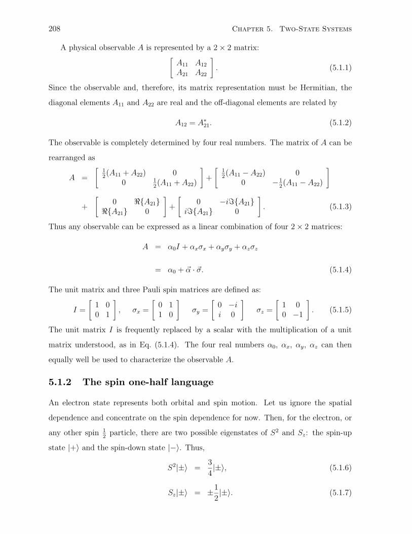
208 Chapter 5. Two-State Systems
A physical observable A is represented by a 2 × 2 matrix:[
A11 A12
A21 A22
]
. (5.1.1)
Since the observable and, therefore, its matrix representation must be Hermitian, the
diagonal elements A11 and A22 are real and the off-diagonal elements are related by
A12 = A∗21. (5.1.2)
The observable is completely determined by four real numbers. The matrix of A can be
rearranged as
A =
[12(A11 + A22) 0
0 12(A11 + A22)
]
+
[12(A11 − A22) 0
0 −12(A11 − A22)
]
+
[0 A21
A21 0
]
+
[0 −iA21
iA21 0
]
. (5.1.3)
Thus any observable can be expressed as a linear combination of four 2 × 2 matrices:
A = α0I + αxσx + αyσy + αzσz
= α0 + α · σ. (5.1.4)
The unit matrix and three Pauli spin matrices are defined as:
I =
[1 00 1
]
, σx =
[0 11 0
]
σy =
[0 −ii 0
]
σz =
[1 00 −1
]
. (5.1.5)
The unit matrix I is frequently replaced by a scalar with the multiplication of a unit
matrix understood, as in Eq. (5.1.4). The four real numbers α0, αx, αy, αz can then
equally well be used to characterize the observable A.
5.1.2 The spin one-half language
An electron state represents both orbital and spin motion. Let us ignore the spatial
dependence and concentrate on the spin dependence for now. Then, for the electron, or
any other spin 12
particle, there are two possible eigenstates of S2 and Sz: the spin-up
state |+〉 and the spin-down state |−〉. Thus,
S2|±〉 =3
4|±〉, (5.1.6)
Sz|±〉 = ±1
2|±〉. (5.1.7)
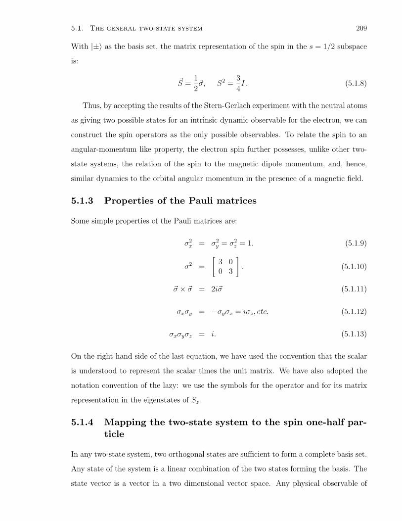
5.1. The general two-state system 209
With |±〉 as the basis set, the matrix representation of the spin in the s = 1/2 subspace
is:
S =1
2σ, S2 =
3
4I. (5.1.8)
Thus, by accepting the results of the Stern-Gerlach experiment with the neutral atoms
as giving two possible states for an intrinsic dynamic observable for the electron, we can
construct the spin operators as the only possible observables. To relate the spin to an
angular-momentum like property, the electron spin further possesses, unlike other two-
state systems, the relation of the spin to the magnetic dipole momentum, and, hence,
similar dynamics to the orbital angular momentum in the presence of a magnetic field.
5.1.3 Properties of the Pauli matrices
Some simple properties of the Pauli matrices are:
σ2x = σ2
y = σ2z = 1. (5.1.9)
σ2 =
[3 00 3
]
. (5.1.10)
σ × σ = 2iσ (5.1.11)
σxσy = −σyσx = iσz, etc. (5.1.12)
σxσyσz = i. (5.1.13)
On the right-hand side of the last equation, we have used the convention that the scalar
is understood to represent the scalar times the unit matrix. We have also adopted the
notation convention of the lazy: we use the symbols for the operator and for its matrix
representation in the eigenstates of Sz.
5.1.4 Mapping the two-state system to the spin one-half par-ticle
In any two-state system, two orthogonal states are sufficient to form a complete basis set.
Any state of the system is a linear combination of the two states forming the basis. The
state vector is a vector in a two dimensional vector space. Any physical observable of
210 Chapter 5. Two-State Systems
the system is represented by a 2× 2 matrix. The two-state systems all have the unifying
features of the same formal structure of the matrix algebra of the two dimensional vector
space for the vector representation of the state and the matrix representation of the
physical observable. Thus, all the two-state systems are said to be isomorphic to the spin
1/2 system. The physical differences among the various two-state systems have to be
found in their basis states or in the coupling of their observables to external stimuli, such
as the electromagnetic fields. Quite commonly, the spin description and terminology are
used for other two-state systems whose properties may have nothing to do with angular
momentum at all. The distinction from the true spin is often made by the term “pseudo-
spin”. The importance of this chapter lies not only in the simplicity which gives us a
graphic illustration of the theory of quantum mechanics, but also in the unified study of
the prototype of many important physical and chemical phenomena.
The most general form of the two-state Hamiltonian is, by Eq. (5.1.4),
H = E0 + B′ · σ, (5.1.14)
completely determined by four real numbers E0, B′x, B′
y, B′z. For the spin 1
2particle, E0
could be the energy of due to its orbital motion. The physical meaning of B ′ is gleaned
from the extension of the classical Hamiltonian of the magnetic dipole moment to the
spin 12
case:
H = E0 − B · µ, (5.1.15)
where B is the external magnetic field. Thus, B′ = µB, where µ is the magnetic dipole
moment of spin 1/2 from µ = µσ. For a nucleon spin, µ is positive,
µ =gsµN
2, (5.1.16)
with µN = eh/2mp for the proton mass mp. For the electron spin, µ is negative,
µ = −µB, (5.1.17)
where we have taken the g-factor to be 2.
5.1. The general two-state system 211
5.1.5 Spin-1/2 Hamiltonian in a magnetic field – redux
In the non-relativistic limit of a particle, the classical kinetic energy is given by
T =p2
2m. (5.1.18)
The quantization procedure consists in replacing p by the momentum operator P with
a spatial representation −ih∇ acting on a wave function ψ(r). To include the spin-
1/2 dynamics, the state vector is written in the basis set of the eigenstates of the spin
component Sz:
ψ =
[ψ+
ψ−
]
. (5.1.19)
The operator equation,
(σ · P )2 = P 2, (5.1.20)
can be established by choosing the z-axis to be along the momentum vector P , leading
to the kinetic energy operator,
T =P 2
2m
[1 00 1
]
=1
2mPzσzσzPz
= (P · σ)1
2m(σ · P ), (5.1.21)
from the vector product invariance. Alternatively, it follows from the relation [see Prob-
lem 5.1 (c)]
( A · σ)( B · σ) = A · B + i( A × B) · σ, (5.1.22)
where σ is a vector of the three Pauli matrices and A and B are two vectors of three
operators.
In the presence of a vector potential A, the momentum P is replaced by P − q A for
the particle with charge q. The kinetic energy operator becomes
T = σ · (P − q A)1
2mσ · (P − q A)
=1
2m(P − q A)2 +
i
2mσ · (P − q A) × (P − q A)
=1
2m(P − q A)2 − qh
2mσ · B, (5.1.23)
212 Chapter 5. Two-State Systems
where we have used the relation (5.1.22), ∇× A = B, and
[P , f(R)] = −ih∇f(r). (5.1.24)
Notice that, for the electron, this gives the correct g factor of 2 for the energy of the spin
magnetic moment in a magnetic field. This is a consequence of the spin transformation
properties and not of relativity.
5.1.6 Examples of two-state systems
We list here examples, besides the electron spin states, and discuss some of them in the
following sections and some in the problems:
1. All spin 12
particles such as neutron and proton.
2. The proton mass is 938.3 MeV/c2 and neutron 939.6 MeV/c2, differing by about 1
part in 103. In the consideration of the nuclear structure consisting of protons and
neutrons, it is convenient to think of the proton and the neutron as two possible
charged states of a particle called the nucleon: when it is charged, it is a proton;
when it is uncharged, it is a neutron. This property of the nucleon is called the
isotopic spin (isospin in short). This terminology is an example of analogy with the
spin 12
system because of the two level nature and not because of any other spin
or angular momentum property. The strong interaction between the two nucleons
conserves the total isospin. This leads to some useful applications, e.g., Problems 14
and 15. Why, then, does one find a mixed neutron and proton state in nature? The
weak electromagnetic interaction breaks the isospin symmetry leading to two stable
charged states and slightly different masses.
3. The dynamics of an atom under the influence of a monochromatic and coherent
radiation field resonant with two levels in the atom is essentially represented by the
two-level atom model. Thus, quantum optics was stimulated by a flow of concepts
from spin resonance.
4. Molecular and solid-state systems which have two low-lying energy states close to
each other but far away from the other excited states. Then, a two-state system
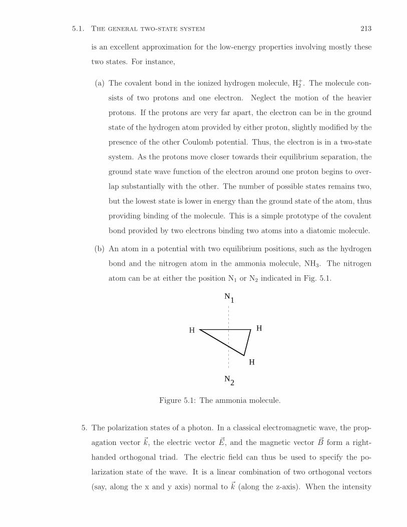
N1
•H
H
H
N2
5.1. The general two-state system 213
is an excellent approximation for the low-energy properties involving mostly these
two states. For instance,
(a) The covalent bond in the ionized hydrogen molecule, H+2 . The molecule con-
sists of two protons and one electron. Neglect the motion of the heavier
protons. If the protons are very far apart, the electron can be in the ground
state of the hydrogen atom provided by either proton, slightly modified by the
presence of the other Coulomb potential. Thus, the electron is in a two-state
system. As the protons move closer towards their equilibrium separation, the
ground state wave function of the electron around one proton begins to over-
lap substantially with the other. The number of possible states remains two,
but the lowest state is lower in energy than the ground state of the atom, thus
providing binding of the molecule. This is a simple prototype of the covalent
bond provided by two electrons binding two atoms into a diatomic molecule.
(b) An atom in a potential with two equilibrium positions, such as the hydrogen
bond and the nitrogen atom in the ammonia molecule, NH3. The nitrogen
atom can be at either the position N1 or N2 indicated in Fig. 5.1.
Figure 5.1: The ammonia molecule.
5. The polarization states of a photon. In a classical electromagnetic wave, the prop-
agation vector k, the electric vector E, and the magnetic vector B form a right-
handed orthogonal triad. The electric field can thus be used to specify the po-
larization state of the wave. It is a linear combination of two orthogonal vectors
(say, along the x and y axis) normal to k (along the z-axis). When the intensity
214 Chapter 5. Two-State Systems
of the electromagnetic wave is so low that it represents a photon, the polarization
state of the photon is then a linear combination of the two states corresponding to
polarization in the x and y direction respectively. Experiments can be carried out
with polaroid films and birefringence crystals.
6. The “strangeness oscillation” of kaons was an important step in the history of ele-
mentary particles and can be understood by the two-state quantum theory without
relativity. From the decay of the long-lived state, the CP violation (breach of the
charge-conjugation and parity invariance) was first found.
5.2 Energy Eigenstates of Spin 12 Particle
5.2.1 Magnetic field splitting
Recall that in the spin 12
system, the basis set chosen consists of the spin up state χ+
and the spin down state χ− which are the eigenstates of σz with eigenvalues +1 and
-1, respectively. In the absence of a magnetic field, these two states are also energy
eigenstates with the same energy E0. In the presence of a magnetic field B, choose, for
convenience, the z-axis along the field direction. From Eq. (5.1.14), the Hamiltonian is
H = E0 + µBBzσz =
[E0 + µBB 0
0 E0 − µBB
]
. (5.2.1)
Since the matrix is already diagonal, it means that χ± remain the energy eigenstates
with energy values E0±µBB. The magnetic field splits the doubly degenerate spin states
into two energy levels with a spacing 2µBB.
5.2.2 Magnetic field in a general direction
Sometimes it is necessary not to choose the z-axis along the direction of the magnetic
field B. Then, the Hamiltonian is
H =
[E0 + µBBz µB(Bx − iBy)
µB(Bx + iBy) E0 − µBBz
]
. (5.2.2)
The diagonalization of this 2 × 2 matrix is straightforward. Nonetheless we record here
a method with which the eigenvalues and eigenstates of a general two-state Hamiltonian
can be easily found. Expressing the magnetic field in the spherical polar coordinates. Let
5.2. Energy Eigenstates of Spin 12 Particle 215
the magnetic field B be in the direction at an angle θ with the z-axis and its projection
in the x-y plane be at an angle φ with the x-axis. Then,
Bx = B sin θ cos φ,
By = B sin θ sin φ,
Bz = B cos θ. (5.2.3)
The Hamiltonian becomes
H = E0
[1 00 1
]
+ µBB
[cos θ sin θe−iφ
sin θeiφ − cos θ
]
. (5.2.4)
We need only diagonalize the second matrix on the right and add E0 to the eigenvalues.
The energy values are
E = E0 ± µBB, (5.2.5)
independent of the direction of the z-axis, as they should be. The corresponding eigen-
states ψ± are given by
[|ψ+〉 |ψ−〉] = [|χ+〉 |χ−〉][
a++ a+−a−+ a−−
]
, (5.2.6)
with the coefficients aij given by,
a++
a−+
=sin θe−iφ
1 − cos θ=
2 sin 12θ cos 1
2θe−iφ
2 sin2 12θ
=cos 1
2θ
sin 12θe−iφ. (5.2.7)
Let us choose the phase of the wave function ψ+ such that
a++ = cos1
2θe−i 1
2φ. (5.2.8)
Then, a−+ = sin1
2θe+i 1
2φ. (5.2.9)
Similarly,
a+− = − sin1
2θe−i 1
2φ, (5.2.10)
a−− = cos1
2θe+i 1
2φ. (5.2.11)
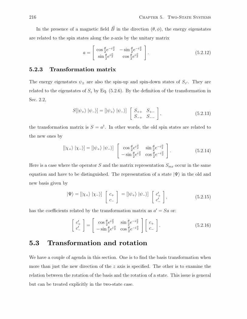
216 Chapter 5. Two-State Systems
In the presence of a magnetic field B in the direction (θ, φ), the energy eigenstates
are related to the spin states along the z-axis by the unitary matrix
a =
cos θ2e−i φ
2 − sin θ2e−i φ
2
sin θ2ei φ
2 cos θ2ei φ
2
. (5.2.12)
5.2.3 Transformation matrix
The energy eigenstates ψ± are also the spin-up and spin-down states of Sz′ . They are
related to the eigenstates of Sz by Eq. (5.2.6). By the definition of the transformation in
Sec. 2.2,
S[|ψ+〉 |ψ−〉] = [|ψ+〉 |ψ−〉][
S++ S+−S−+ S−−
]
, (5.2.13)
the transformation matrix is S = a†. In other words, the old spin states are related to
the new ones by
[|χ+〉 |χ−〉] = [|ψ+〉 |ψ−〉]
cos θ2ei φ
2 sin θ2e−i φ
2
− sin θ2ei φ
2 cos θ2e−i φ
2
. (5.2.14)
Here is a case where the operator S and the matrix representation Smx occur in the same
equation and have to be distinguished. The representation of a state |Ψ〉 in the old and
new basis given by
|Ψ〉 = [|χ+〉 |χ−〉][
c+
c−
]= [|ψ+〉 |ψ−〉]
[c′+c′−
]
, (5.2.15)
has the coefficients related by the transformation matrix as a′ = Sa or:
[c′+c′−
]
=
cos θ2ei φ
2 sin θ2e−i φ
2
− sin θ2ei φ
2 cos θ2e−i φ
2
[c+
c−
]
. (5.2.16)
5.3 Transformation and rotation
We have a couple of agenda in this section. One is to find the basis transformation when
more than just the new direction of the z axis is specified. The other is to examine the
relation between the rotation of the basis and the rotation of a state. This issue is general
but can be treated explicitly in the two-state case.
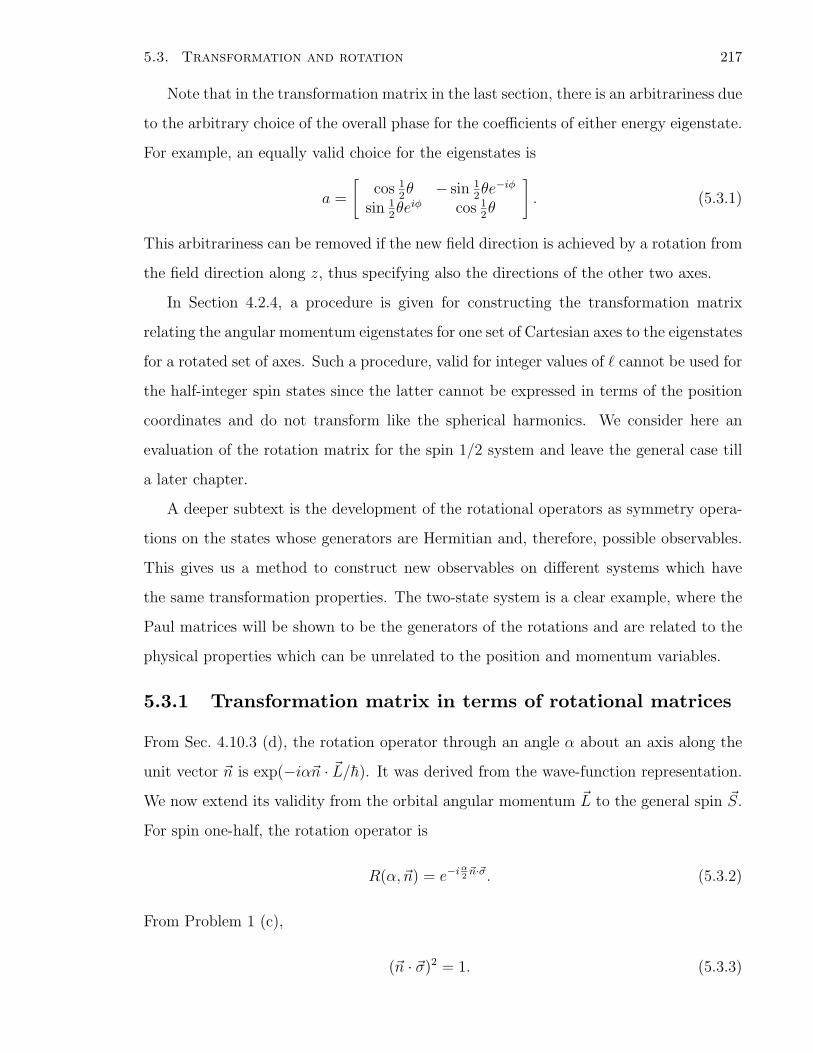
5.3. Transformation and rotation 217
Note that in the transformation matrix in the last section, there is an arbitrariness due
to the arbitrary choice of the overall phase for the coefficients of either energy eigenstate.
For example, an equally valid choice for the eigenstates is
a =
[cos 1
2θ − sin 1
2θe−iφ
sin 12θeiφ cos 1
2θ
]
. (5.3.1)
This arbitrariness can be removed if the new field direction is achieved by a rotation from
the field direction along z, thus specifying also the directions of the other two axes.
In Section 4.2.4, a procedure is given for constructing the transformation matrix
relating the angular momentum eigenstates for one set of Cartesian axes to the eigenstates
for a rotated set of axes. Such a procedure, valid for integer values of cannot be used for
the half-integer spin states since the latter cannot be expressed in terms of the position
coordinates and do not transform like the spherical harmonics. We consider here an
evaluation of the rotation matrix for the spin 1/2 system and leave the general case till
a later chapter.
A deeper subtext is the development of the rotational operators as symmetry opera-
tions on the states whose generators are Hermitian and, therefore, possible observables.
This gives us a method to construct new observables on different systems which have
the same transformation properties. The two-state system is a clear example, where the
Paul matrices will be shown to be the generators of the rotations and are related to the
physical properties which can be unrelated to the position and momentum variables.
5.3.1 Transformation matrix in terms of rotational matrices
From Sec. 4.10.3 (d), the rotation operator through an angle α about an axis along the
unit vector n is exp(−iαn · L/h). It was derived from the wave-function representation.
We now extend its validity from the orbital angular momentum L to the general spin S.
For spin one-half, the rotation operator is
R(α,n) = e−i α2n·σ. (5.3.2)
From Problem 1 (c),
(n · σ)2 = 1. (5.3.3)
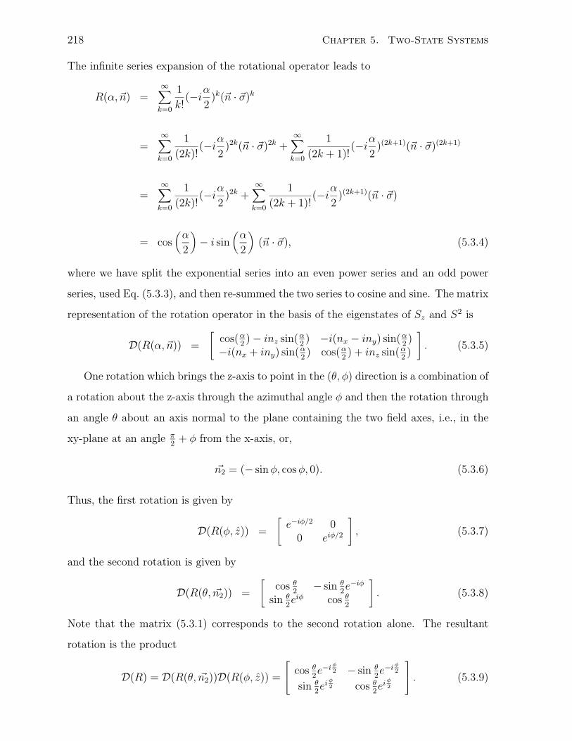
218 Chapter 5. Two-State Systems
The infinite series expansion of the rotational operator leads to
R(α,n) =∞∑
k=0
1
k!(−i
α
2)k(n · σ)k
=∞∑
k=0
1
(2k)!(−i
α
2)2k(n · σ)2k +
∞∑
k=0
1
(2k + 1)!(−i
α
2)(2k+1)(n · σ)(2k+1)
=∞∑
k=0
1
(2k)!(−i
α
2)2k +
∞∑
k=0
1
(2k + 1)!(−i
α
2)(2k+1)(n · σ)
= cos(
α
2
)
− i sin(
α
2
)
(n · σ), (5.3.4)
where we have split the exponential series into an even power series and an odd power
series, used Eq. (5.3.3), and then re-summed the two series to cosine and sine. The matrix
representation of the rotation operator in the basis of the eigenstates of Sz and S2 is
D(R(α,n)) =
[cos(α
2) − inz sin(α
2) −i(nx − iny) sin(α
2)
−i(nx + iny) sin(α2) cos(α
2) + inz sin(α
2)
]
. (5.3.5)
One rotation which brings the z-axis to point in the (θ, φ) direction is a combination of
a rotation about the z-axis through the azimuthal angle φ and then the rotation through
an angle θ about an axis normal to the plane containing the two field axes, i.e., in the
xy-plane at an angle π2
+ φ from the x-axis, or,
n2 = (− sin φ, cos φ, 0). (5.3.6)
Thus, the first rotation is given by
D(R(φ, z)) =
[e−iφ/2 0
0 eiφ/2
]
, (5.3.7)
and the second rotation is given by
D(R(θ, n2)) =
[cos θ
2− sin θ
2e−iφ
sin θ2eiφ cos θ
2
]
. (5.3.8)
Note that the matrix (5.3.1) corresponds to the second rotation alone. The resultant
rotation is the product
D(R) = D(R(θ, n2))D(R(φ, z)) =
cos θ2e−i φ
2 − sin θ2e−i φ
2
sin θ2ei φ
2 cos θ2ei φ
2
. (5.3.9)
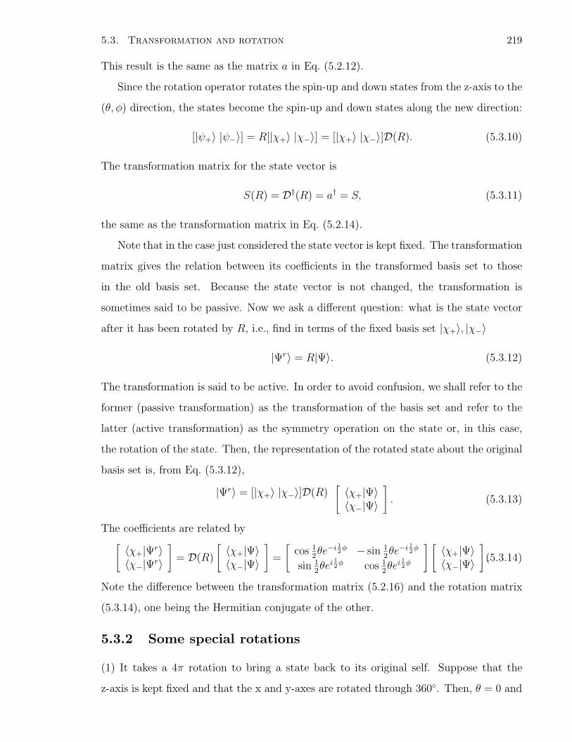
5.3. Transformation and rotation 219
This result is the same as the matrix a in Eq. (5.2.12).
Since the rotation operator rotates the spin-up and down states from the z-axis to the
(θ, φ) direction, the states become the spin-up and down states along the new direction:
[|ψ+〉 |ψ−〉] = R[|χ+〉 |χ−〉] = [|χ+〉 |χ−〉]D(R). (5.3.10)
The transformation matrix for the state vector is
S(R) = D†(R) = a† = S, (5.3.11)
the same as the transformation matrix in Eq. (5.2.14).
Note that in the case just considered the state vector is kept fixed. The transformation
matrix gives the relation between its coefficients in the transformed basis set to those
in the old basis set. Because the state vector is not changed, the transformation is
sometimes said to be passive. Now we ask a different question: what is the state vector
after it has been rotated by R, i.e., find in terms of the fixed basis set |χ+〉, |χ−〉
|Ψr〉 = R|Ψ〉. (5.3.12)
The transformation is said to be active. In order to avoid confusion, we shall refer to the
former (passive transformation) as the transformation of the basis set and refer to the
latter (active transformation) as the symmetry operation on the state or, in this case,
the rotation of the state. Then, the representation of the rotated state about the original
basis set is, from Eq. (5.3.12),
|Ψr〉 = [|χ+〉 |χ−〉]D(R)[〈χ+|Ψ〉〈χ−|Ψ〉
]
. (5.3.13)
The coefficients are related by[〈χ+|Ψr〉〈χ−|Ψr〉
]
= D(R)
[〈χ+|Ψ〉〈χ−|Ψ〉
]
=
[cos 1
2θe−i 1
2φ − sin 1
2θe−i 1
2φ
sin 12θei 1
2φ cos 1
2θei 1
2φ
] [〈χ+|Ψ〉〈χ−|Ψ〉
]
.(5.3.14)
Note the difference between the transformation matrix (5.2.16) and the rotation matrix
(5.3.14), one being the Hermitian conjugate of the other.
5.3.2 Some special rotations
(1) It takes a 4π rotation to bring a state back to its original self. Suppose that the
z-axis is kept fixed and that the x and y-axes are rotated through 360. Then, θ = 0 and
220 Chapter 5. Two-State Systems
φ = 2π. From Eq. (5.3.1) or Eq. (5.2.12),
|ψ±〉 = −|χ±〉. (5.3.15)
The spin 12
wave functions change sign, but the probability is the same. The sign change
may be regarded as a phase change of π. This is an example where the overall phase of
a wave function cannot be measured. However, if it is made to interfere with another
part of the wave function, such as in the neutron interference setup of Problem 17, the
phase difference between a part which is not changed and a part which is changed may
be detected. The experiment was first suggested by Herbert J. Bernstein and performed
by S.A. Werner et al.
(2) The z′-axis points opposite the z-axis. Then, θ = π and φ = 0. From Eq. (5.3.8),
|ψ+〉 = |χ−〉, (5.3.16)
|ψ−〉 = −|χ+〉. (5.3.17)
The spin-up and down states are interchanged as expected but one of the states also
changes sign.
5.4 Spin Precession
When a spin 12
particle is placed in a magnetic field, the energy eigenstates are the spin-
up and spin-down states in the direction of the field. If the particle is in one of these
states, it will stay in the same state forever, provided it is well isolated. Now we wish
to find the time development of the spin state if the initial state is known and is not
necessarily in one of the energy eigenstates.
For convenience, consider the electron and measure energy from E0. Let the z-axis
be along the magnetic field B. The spin up and down states χ± are also the energy
eigenstates. Suppose that at t = 0, the spin points in the θ, φ direction with respect to
the chosen axes. This is putting it in a picturesque way. To be precise, we mean that the
initial state of the particle is in the spin-up eigenstate of the component of spin S along
the θ, φ direction. From Eq. (5.2.6) and Eq. (5.2.12) the spin state of the electron is at
5.4. Spin Precession 221
t = 0,
|Ψ(0)〉 = |χ+〉 cosθ
2e−i φ
2 + |χ−〉 sinθ
2ei φ
2 . (5.4.1)
Since χ± are also energy eigenstates in the presence of the field B, the state at time
t is
|Ψ(t)〉 = |χ+〉 cosθ
2e−i φ
2−iµBBt/h + |χ−〉 sin
θ
2ei φ
2+iµBBt/h, (5.4.2)
where ±µBB are the energy values of χ±. Notice that the wave function at time t has
exactly the same form as at t = 0 if φ is changed to φ + ω0t, where
ω0 = 2µBB/h. (5.4.3)
Thus, the state of the particle, |Ψ(t)〉, is the spin-up state along the direction θ, φ + ω0t.
When the particle is in the spin-up state of the component of the spin along a certain
direction, as a shorthand and as a helpful mental picture we say and think that the
spin vector of the particle is pointing in that direction. Thus, the dynamics of the spin
1/2 state may be traced on the unit sphere, known as the Bloch sphere, in honor of
Felix Bloch’s pioneering work on spin dynamics, which included the Bloch equation in
Problem 4. Note that this is not at all the same picture as the one described in the vector
model. If the spin initially points at an angle θ from the z-axis, the angle of the spin
vector remains the same at all times. The angle φ, which its (classical) projection makes
with the x-axis, will increase at a constant rate ω0. The spin vector precesses about the
z-axis, which is the direction of the magnetic field, with a constant angular frequency ω0.
2µB/h = 1.8 × 10¹¹sec−1tesla−1
= 2.8 × 10¹⁰hertz tesla−1
= 1.8 × 10⁷sec−1gauss−1. (5.4.4)
For a field of about 100 gauss, the precession frequency is 2× 10⁹sec−1 or about 108 Hz,
which is in the range of the microwave frequencies.
222 Chapter 5. Two-State Systems
5.4.1 Spin flip
If we know the direction of a spin, we can in principle flip it through 180 (changing it
from a spin-up state in that direction to a spin-down state) by turning on a field B at
right angles to the spin for a time π/ω0, i.e., half a precession cycle, and then turning
the field off (known as the π-pulse).
5.5 Magnetic Resonance
A uniform static magnetic field B0 along the z-axis will split the spin-up and spin-down
states’ energy apart with a gap 2µBB0. At low enough temperatures, the electron will
stay in the lower energy state, i.e., the spin-down state. Now supply the system with
energy from an electromagnetic wave of frequency ω. If ω is equal to the precession
frequency, i.e.,
ω = ω0 = 2µBB0/h, (5.5.1)
the electron can absorb a photon of energy hω and get excited to the higher energy state,
i.e., the spin-up state. This absorption of the electromagnetic energy at a particular
frequency is called the magnetic resonance.
The magnetic resonance can also be described in terms of the time dependent picture
developed in the last two sections. When the field B0 is applied to the system, the electron
spin will in general be at an angle with the field direction. The spin will, therefore, precess
about the field with frequency ω0. Now apply a small circularly polarized rf field with
the magnetic field in the plane at right angles to the static field B0. If the frequency of
the rf field is in resonance with the precession rate, the rf magnetic field vector is fixed in
the rotating frame of the spin vector. The rf field can then rotate the spin vector. How
this secondary precession leads to a transition between two spin states is studied next.
5.5.1 Transition probability
We have a qualitative picture of magnetic resonance and also the resonance condition
(5.5.1). In principle, we know how to obtain the time dependence of the transition of
the spin-1/2 particle from the spin-down state to the spin-up state. In this subsection,
5.5. Magnetic Resonance 223
we study the case of the weak perturbing field (compared to the static field producing
the energy splitting) with a broad bandwidth which yields a quantitative account of the
probability of transition. In the next section, we shall study by contrast the case of a
strong perturbing oscillating field with a narrow frequency spectrum.
Let the oscillating magnetic field be perpendicular to the static field B0, thus:
Bx = b cos ωt,By = b sin ωt,Bz = B0.
(5.5.2)
We have chosen the oscillating field to be right-handed circularly polarized for clarity of
exposition. The justification of this term being dominant in near-resonance condition is
given below. The oscillating field which supplies energy to the electron is assumed to be
small compared with the static field: b B0.
The Hamiltonian of the electron in the presence of the static field B0 is
H0 =
[µB B0 00 −µB B0
]
. (5.5.3)
The oscillating field provides a perturbation on the Hamiltonian,
H1 =
[0 µBbe−iωt
µBbeiωt 0
]
. (5.5.4)
The total Hamiltonian of the electron is the sum
H = H0 + H1. (5.5.5)
The matrix representations above refer to the basis set of the spin up and down states
|χ±〉 along the z-axis, i.e., the direction of the static field B0.
Let the state of the electron spin at time t be
|Ψ(t)〉 = |χ+〉a+(t) + |χ−〉a−(t). (5.5.6)
The Schrodinger equation
ih∂|Ψ〉∂t
= H|Ψ〉, (5.5.7)
can easily be written in matrix form by noting that |Ψ(t)〉 is represented by a column
vector and H by a matrix, and, thus,
ihda+
dt= H++a+ + H+−a−, (5.5.8)
224 Chapter 5. Two-State Systems
ihda−dt
= H−+a+ + H−−a−. (5.5.9)
The solution of the Schrodinger equation in either form is facilitated by the transfor-
mation to the interaction representation for the state,
|Ψ(t)〉 = e−iH0t/h|Φ(t)〉, (5.5.10)
and for the observable A,
A(t) = eiH0t/h A e−iH0t/h. (5.5.11)
If there were no perturbation (H1 = 0), then |Φ(t)〉 would be time independent and the
observable would be in the Heisenberg representation. The interaction representation
simplifies the Schrodinger equation in the presence of the perturbation to
ih∂|Φ(t)〉
∂t= H1(t)|Φ(t)〉, (5.5.12)
In the matrix representation, if c±(t) denotes the coefficients of |Φ(t)〉, then
a+(t) = c+(t)e−iE+t/h (5.5.13)
a−(t) = c−(t)e−iE−t/h, (5.5.14)
where, E± = ±µBB0, (5.5.15)
are the energies of the spin states in the presence of the static field B0 only. The
Schrodinger equation in the interaction representation becomes
ihdc+
dt= µBbe−i(ω−ω0)tc−, (5.5.16)
ihdc−dt
= µBbei(ω−ω0)tc+, (5.5.17)
where ω0 is the precession frequency
ω0 = (E+ − E−)/h = 2µBB0/h. (5.5.18)
5.5. Magnetic Resonance 225
The two equations are coupled by the rf field b. Suppose that the application of the
rf field starts at t = 0 when the electron is in the lower energy state, i.e., the spin-down
state:
c+(0) = 0,c−(0) = 1.
(5.5.19)
Since the rf field is weak compared with the static field B0, as the time goes on, the
change of the probability amplitudes c+(t) and c−(t) will be of the order b/B0.
The smallness of b/B0 enables us to solve Eqs. (5.5.16) - (5.5.17), approximately.
Since c+(t) will be of the order of b/B0, we may substitute for c−(t) on the right-hand
side of Eq. (5.5.16) its initial value of unity with an error on the right of O(b/B0)2.
ihdc+
dt= µBbe−i(ω−ω0)t. (5.5.20)
Hence,
c+(t) =µBb/h
ω − ω0
[e−i(ω−ω0)t − 1]
= − µBb/h
ω − ω0
e−i 12(ω−ω0)t2i sin
[1
2(ω − ω0)t
]
. (5.5.21)
The probability of transition from the spin-down state χ− to the spin-up state χ+ at
time t is
P−+(ω) = |c+(t)|2
= (µbt/h)2
[sin 1
2(ω − ω0)t
12(ω − ω0)t
]2
. (5.5.22)
For a given time t, the transition probability as a function of the exciting field frequency
ω is sharply peaked at the resonance frequency ω0, as shown in Fig. 5.2. For a field B0
of about 100 gauss, the resonance frequency ω0 is 2 × 10⁹sec−1. If we use a reasonable
time scale of 10−2 sec, the width of the resonance peak is about
∆ω = π/t 3 × 10²sec−1. (5.5.23)
The Q of the resonance is
Q = ω0/∆ω = 107, (5.5.24)
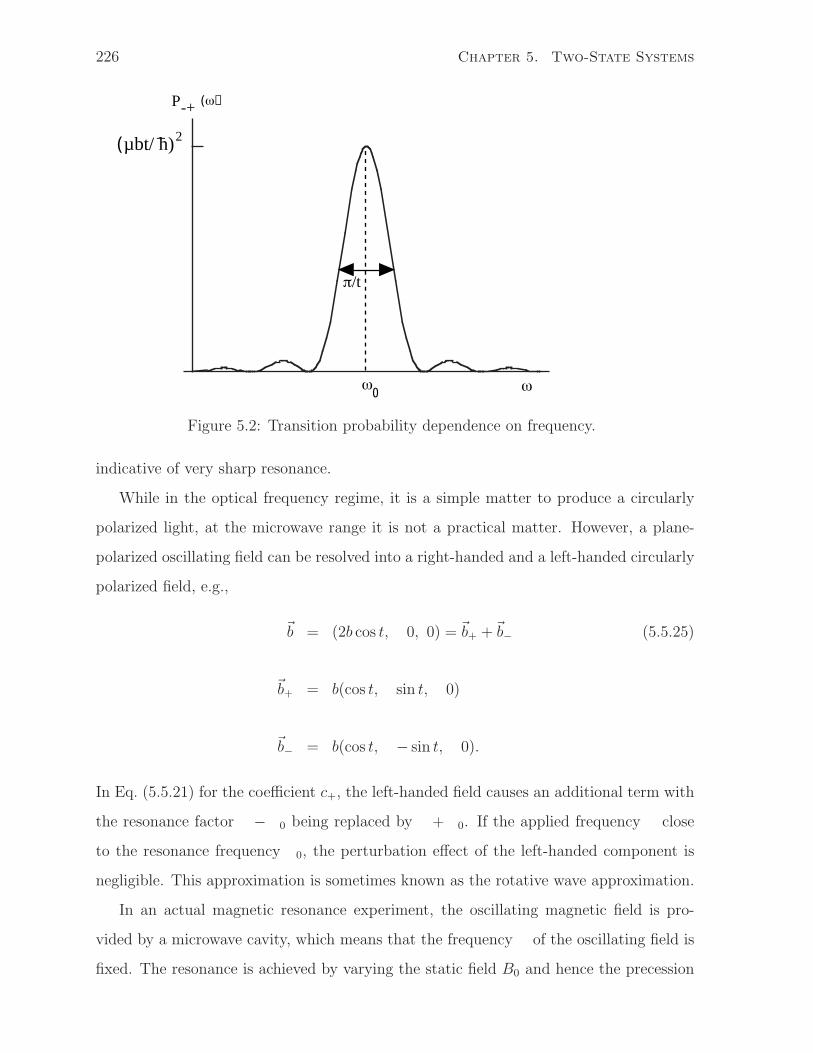
ωω0
(µbt/ h)_ 2
P-+ (ω)
π/t
226 Chapter 5. Two-State Systems
Figure 5.2: Transition probability dependence on frequency.
indicative of very sharp resonance.
While in the optical frequency regime, it is a simple matter to produce a circularly
polarized light, at the microwave range it is not a practical matter. However, a plane-
polarized oscillating field can be resolved into a right-handed and a left-handed circularly
polarized field, e.g.,
b = (2b cos ωt, 0, 0) = b+ +b− (5.5.25)
b+ = b(cos ωt, sin ωt, 0)
b− = b(cos ωt, − sin ωt, 0).
In Eq. (5.5.21) for the coefficient c+, the left-handed field causes an additional term with
the resonance factor ω − ω0 being replaced by ω + ω0. If the applied frequency ω close
to the resonance frequency ω0, the perturbation effect of the left-handed component is
negligible. This approximation is sometimes known as the rotative wave approximation.
In an actual magnetic resonance experiment, the oscillating magnetic field is pro-
vided by a microwave cavity, which means that the frequency ω of the oscillating field is
fixed. The resonance is achieved by varying the static field B0 and hence the precession
5.5. Magnetic Resonance 227
frequency ω0. Knowing the g-factor of the electron spin, this experiment gives a more
accurate measurement of the Bohr magneton than the Stern-Gerlach experiment.
The microwave cavity has a finite band width, which is easily greater than the natural
width π/t of the resonance given by Eq. (5.5.22). Let the intensity of the microwave per
unit frequency range ω be hb2I(ω), where I(ω), the density of states for a unit magnetic
field, is a much more slowly varying function of ω than the transition probability (5.5.22).
Then, the total probability over all frequencies for the transition from the spin-down state
to the spin-up state at time t is
P−+ =∫ ∞
0dω(µBbt/h)2hI(ω)
[sin 1
2(ω − ω0)t
12(ω − ω0)t
]2
=2π
h(µBb)2I(ω0)t, (5.5.26)
where we have replaced I(ω) under the integral by I(ω0) since it varies negligibly over
the range of π/t around the resonance frequency ω0.
The transition probability per unit time is, therefore,
Q−+ =2π
h|〈χ−|H1|χ+〉|2I(ω0), (5.5.27)
where we have used Eq. (5.5.4) for the perturbation H1. This formula is known as the
Fermi golden rule. It has the form of the general formula for the transition probability per
unit time between two states due to a perturbation H1. A small but important difference
with the more common formula lies in the density of states of the system in place of the
cavity intensity distribution. The difference in physics comes from the assumption here
that the two unperturbed energy states are infinitely sharp (or have infinite life-time)
whereas the usual derivation makes use of the broad energy distribution. A derivation of
more general validity will be given in the chapter on perturbation theory.
The resonance phenomenon is not restricted to the spin 12
states of the electron.
Clearly, any two level system can have resonance. In particular, the magnetic resonance
due to the spin of nuclear particles is possible (known as the nuclear magnetic resonance),
even though compared with the electron spin resonance the transition probability per
unit time is down by a factor of at least 106 because of the dependence on the square
of the magnetic dipole moment. Also, any magnetic dipole moment, whether it comes
228 Chapter 5. Two-State Systems
from the spin or orbital angular momentum, precesses about a static magnetic field and,
therefore, has resonance if excited by an oscillating field. For any angular momentum,
spin or orbital, greater than a half, there are more than two states and there is more
than one resonance between two adjacent energy levels.
5.5.2 The Rabi oscillations
Actually, the equations of motion reduced to Eqs. (5.5.16) and (5.5.17) can be solved
exactly for any strength of the ac field b in the circular polarization. This solution
will give us not only the phenomenon of Rabi oscillation which is of importance to
nuclear magnetic resonance, quantum optics, and quantum computing, but also gives us
a perspective to the perturbation theory of quantum transitions by examining an exact
solution of a nontrivial model problem.
Let us introduce two quantities which help to make the physics of the solution more
transparent. One is the detuning,
δ = ω0 − ω, (5.5.28)
the difference between the frequency of the driving field and the characteristic frequency
of the two-level system. The other is the Rabi frequency
ΩR = 2µBb/h (5.5.29)
which is also a measure of the strength of the driving field. Eqs. (5.5.16) and (5.5.17)
become
idc+
dt=
ΩR
2e−iδtc−,
idc−dt
=ΩR
2eiδtc+. (5.5.30)
A transformation of the coefficients of the state
c+ = b+e−iδt/2, c− = b−eiδt/2, (5.5.31)
eliminates the explicit time dependence in the equations,
id
dt
[b+
b−
]
=1
2
[δ ΩR
ΩR −δ
] [b+
b−
]
. (5.5.32)
5.5. Magnetic Resonance 229
The transformation (5.5.31) may be viewed as one into a rotating frame with relative
angular velocity δ as can be deduced from Eq. (5.4.2). The resultant equation (5.5.32) has
the same form as the Schrodinger equation with a constant potential. The time evolution
of the transformed state can be solved in the standard way in terms of the eigenstates.
We use the spin analogy to diagonalize the pseudo-Hamiltonian in the rotating frame on
the right side of Eq. (5.5.32) and let
Ω =√
δ2 + Ω2R
cos θ = δ/Ω. (5.5.33)
The eigenstates associated with the eigenvalues ±Ω/2 are, respectively,
ψ+ =
[b++
b+−
]
=
[cos θ
2
sin θ2
]
ψ− =
[b−+
b−−
]
=
[− sin θ
2
cos θ2
]
. (5.5.34)
The initial condition of the system being in the lower state leads to the time evolution,
[b+
b−
]
= ψ+ sinθ
2e−iΩt/2 + ψ− cos
θ
2eiΩt/2. (5.5.35)
The state in the interaction representation is
[c+
c−
]
=
[−i sin θ sin(Ωt/2)e−iδt/2
cos(Ωt/2) + i cos θ sin(Ωt/2)eiδt/2
]
. (5.5.36)
We have deliberately adopted an elementary mathematical procedure to solve the Rabi
oscillation problem here. In Problem 7, a more concise approach is used to yield a
geometrical description of the spin dynamics in terms of an rf-field driven rotation in a
precessing frame caused by the static magnetic field.
After applying the right-handed circularly polarized field to the spin in its ground
state, the probability of find the spin in the spin-up state at time t is
P−+(t) = |c+|2 =1
2sin2 θ [1 − cos(Ωt)] , (5.5.37)
oscillating with the Rabi frequency. When there is a finite detuning (sin2 θ < 1), even
at maximum transition probability the state is not entirely in the spin-up state. The
230 Chapter 5. Two-State Systems
expectation value of the longitudinal component of the dipole moment
〈µz〉 = −µB〈Ψ(t)|σz|Ψ(t)〉 = −µB(|c+|2 − |c−|2) = µB[cos2 θ + sin2 θ cos(Ωt)].(5.5.38)
In the case of laser action, this is a measure of the population inversion. The transverse
magnetization may be obtained from
〈µ+〉 = 〈µx + iµy〉 = −µB〈Ψ(t)|σ+|Ψ(t)〉 = −2µBa∗+a−
= −2µB sin θ sinΩt
2
(
cos θ sinΩt
2+ i cos
Ωt
2
)
eiωt. (5.5.39)
The factor eiωt shows the interesting fact that the transverse magnetization can be phase-
locked with the driving field. The Rabi oscillation opens up the possibility of making an
arbitrary combination of the two states (not just making the transition from one state
to another with a finite probability). This is a fundamental requirement for quantum
computation and quantum information processing.
5.5.3 Irreversible transitions versus oscillations between states
We now address the fundamental difference between the Fermi golden rule and the
Rabi oscillation. The exact solution in Eq. (5.5.36) does contain the weak field limit
in Eq. (5.5.21). To reach the Fermi rule, we then include the contribution of the driving
fields with frequencies in the neighborhood of the resonance frequency (or alternately
include the finite lifetime of the final state or the finite state distribution around it). In
the long-time limit, the destructive interference of the neighboring nonresonant contribu-
tions converts the oscillations into an irreversible transition. The requirement of the Rabi
oscillations is that the driving frequency is sharp and the level life-time is so long that the
coherent effects of the oscillations are visible. Eventually, in a realistic system, the de-
coherence effects (treated in the next section) will diminish the Rabi oscillations. Thus,
the apparent contradiction between the appearance of the abrupt jumps in the Fermi
golden rule and the seemingly deterministic motion of the Rabi oscillations is resolved as
the two limits of frequency resolution of the driving field.
5.6. Dissipative Dynamics for an Ensemble of Two-Level Systems 231
5.6 Dissipative Dynamics for an Ensemble of Two-Level Systems
The density matrix for an ensemble of two-level systems is the tool for describing the
state in dynamics with dissipation. As we have seen above, there are many important
two-level systems, and thus the density matrix for the two-level systems has applications
in many areas, particularly the electron and nuclear spin resonance and quantum optics
in which the two-level atom model is basic. For convenience and for historical reasons,
the terminology for the general two-level system is still couched in terms of the spin 1/2
system.
5.6.1 The Bloch equations
The Hamiltonian of the two-state system consists of two parts,
H = H0 + H1, (5.6.1)
where H0 is the conservative part with the form (5.5.3) containing the static field B0
chosen to be in the z direction and H1 is driven by a time-dependent field b = (bx, by, bz),
not necessarily of the circularly polarized transverse field (5.5.4). When the influence of
the environment is included, the description of the dissipative dynamics, from Section
2.6.6, is given by the master equation for the density matrix,
d
dtρ(t) =
1
ih[H, ρ] +
d
dtρ(t)
∣∣∣∣∣relax
, (5.6.2)
where the relaxation terms have the form
d
dt
[ρ++ ρ+−ρ−+ ρ−−
]
relax=
Γaρ−− − Γeρ++ −
12(Γa + Γe) + Γ∗
ρ+−
−
12(Γa + Γe) + Γ∗
ρ−+ −Γaρ−− + Γeρ++
,(5.6.3)
in the spin basis set (|+〉, |−〉), with the |−〉 being the ground state. The absorption rate
and emission rate are, respectively, Γa, Γe and the pure dephasing rate Γ∗.
The 2 × 2 density matrix still obeys the unit trace constraint. It can, therefore, be
put in the form
ρ =1
2(I + P · σ), (5.6.4)
232 Chapter 5. Two-State Systems
where P is a vector of three numbers known as the spin polarization in a spin system
or simply polarization in a general two-state system such as the atom model (in which
case it should not be confused with the polarization vector of the photon). The ensemble
average of the spin vector is given by S = P/2.
In the most general construction of the density matrix which is determined by the
fractions 12(1 + P ) and 1
2(1 − P ) for the spin up and down states in the (θ, φ) direction,
the density matrix in the basis of the spin up and down states along the z direction is
ρ =1
2
[1 + P cos θ P sin θe−iφ
P sin θeiφ 1 − P cos θ
]
=1
2
[1 + Pz Px − iPy
Px + iPy 1 − Pz
]
. (5.6.5)
The parameters (P, θ, φ) and (Px, Py, Pz) are just the polar and Cartesian coordinates of
the vector P .
From the above master equation of the density matrix, it is possible to derive the
equation of motion for the spin polarization P , known as the Bloch equation, (see Prob-
lem 4),
dP
dt= γ P × B − 1
T1
(P‖ − P0
)− 1
T2
P⊥, (5.6.6)
where γ = µ/h is the gyromagnetic ratio. P‖ = (0, 0, Pz) is the longitudinal component
of the polarization at time t and P⊥ = (Px, Py, 0) is the transverse component. The
time-independent P0 is the steady state value when H1 is zero, given by (0, 0, P0) where,
P0 = −Γe − Γa
Γe + Γa
. (5.6.7)
The decay time T1, given by
1
T1
= Γe + Γa, (5.6.8)
is known as the longitudinal relaxation time. It is a measure of the relaxation time of
the longitudinal component of the polarization P‖ to P0. The decay time T2, given by,
1
T2
=1
2(Γe + Γa) + Γ∗, (5.6.9)
is the transverse relaxation time (or the decoherence time). It is a measure of the relax-
ation time of the transverse component of the polarization P⊥.
Thus, the physical picture of spin precession about a magnetic field and spin flipping,
etc, applies not only to a pure spin state but also to the average spin vector of an ensemble
of spins or other two-level systems. Problem 3 derives a number of these properties.
5.6. Dissipative Dynamics for an Ensemble of Two-Level Systems 233
5.6.2 Relaxation times due to transitions between states
We have obtained the form of the decay terms from the Lindblad form. Here we shall
examine the physical origin of the Γa and Γe terms in the damping or relaxation rates.
We choose the example where the two-state atom is driven by an oscillating field (see
Problem 9) and is coupled to the reservoir of the ambient electromagnetic fields. While
the radiative transition is important to the decaying processes in a two-level atom, it
is not the dominant relaxation mechanism for an electron spin situated in a vibrating
lattice, where the phonons or the random interaction with other spins are generally
more important. The treatment is meant to be illustrative rather than exhaustive of the
microscopic relaxation mechanisms.
From the Lindblad generator√
Γa|+〉〈−|, we identify the process as the transition
of the system from the ground state absorbing a photon or electromagnetic energy from
the electromagnetic reservoir. Similarly, Γe is identified as the emission rate. There are
two ways to derive formulas for these two rates. One way is to treat the electromagnetic
field in the reservoir quantum mechanically as photons. The other is to treat the fields
as classical quantities, except that the energy density obeys Planck’s law. The second
method, coupled with the quantum treatment of the system, is known as the semiclassical
method.
The quantum treatment will be given in Chapter 14. The essence of the physics
lies in quantizing the electromagnetic field into the photons the same way the harmonic
oscillator is quantized into phonons. From the well-known transition relations between
the harmonic oscillator states, c†|n〉 =√
n + 1|n+1〉 and c|n〉 =√
n|n−1〉, the absorption
process from the ground state to the excited state of the two-level atom will take a photon
away from the reservoir with the probability proportional to n (the relevant matrix
element squared) while the emission process from the excited state to the excited state of
the two-level atom will give a photon to the reservoir with the probability proportional
to n + 1. The thermal average of n at frequency ω in a thermodynamic equilibrium at
temperature T is given by (see Problem 3.6)
n(ω) =1
ehω/kBT − 1, (5.6.10)
where kB is the Boltzmann constant. The two relaxation rates may be calculated by the
234 Chapter 5. Two-State Systems
Fermi Golden Rule. Since the transition matrix elements for the system part are the
same for emission and absorption,
Γe
Γa
=n(ω) + 1
n(ω). (5.6.11)
Hence, the emission rate may be considered as composed of a stimulated term (proportion
to the number of relevant photons in the reservoir, n(ω)) and a spontaneous term,
Γs = Γe − Γa. (5.6.12)
With the formula for the spontaneous emission rate Γs, Eq. (14.8.9), the absorption and
emission rates are
Γa = Γsn(ω), (5.6.13)
Γe = Γsn(ω) + 1. (5.6.14)
The semiclassical treatment is due to Einstein. It is included here because the physical
argument is illuminating. The essence of the physics is to use the thermal equilibrium
of the reservoir to relate the emission rate and the absorption rate to temperature. If
the system with the steady state polarization (0, 0, P0) is in thermal equilibrium with the
reservoir at temperature T , then the Boltzmann law says that the ratio of the probabilities
being in states |+〉 and |−〉 is
ρ++
ρ−−=
1 + P0
1 − P0
= e−hω/kBT . (5.6.15)
If we let Γs = Γe − Γa, the relation Eq. (5.6.7) of P0 to Γa and Γe yields the formulas,
Γa = Γsn(ω) (5.6.16)
Γe = Γs[n(ω) + 1], (5.6.17)
where the thermal distribution of photons n(ω), as defined by Eq. (5.6.10), is a result of
the Einstein argument.
Section (5.5.1) gives the transition rate from the ground state to the excited state in
Eq.(5.5.27). For the electrical field excitation, the formula is
Γa =2π
h|〈+|H1|−〉|2I(hω), (5.6.18)
5.6. Dissipative Dynamics for an Ensemble of Two-Level Systems 235
where hω is the energy difference between the two states and the transition matrix
element is 〈+|H1|−〉 = µ · E , with the electric dipole moment µ and the density of states
per unit energy per polarization for the photon reservoir is, from Problem 3.9, given by
I(hω) =ω2
2π2hc3. (5.6.19)
To relate Γa to the transition rate, we average the latter over all possible directions of
the polarization vector so that the matrix element squared yields a factor of 13µ2E2. By
Planck’s theory, we replace the classical energy density by the phonon one,
ε0E2I(E) = hωn(ω)ω2
hπ2c3. (5.6.20)
Thus, the semiclassical treatment of the decay rate Γa leads to
Γs =µ2ω3
3πε0hc3. (5.6.21)
If we calculate the transition rate from state |+〉 to |−〉 driven by the oscillating electric
field by the same perturbative method as the absorption process, we would get the same
decay rate as Γa. This is known as the principle of microscopic balance. The extra
term Γs in the emission rate Γe, Eq. (5.6.17), is independent of the applied electric
field and is known as the spontaneous emission rate. By contrast, the Γsn(ω) is known
as the stimulated emission rate. Although Γs comes of the semiclassical argument, its
true physical origin derives from the quantization of the electromagnetic field yielding a
vacuum field.
5.6.3 A physical origin of pure dephasing
The Lindblad term√
2Γ∗|+〉〈+| leads to a decay rate Γ∗ only of the coherence term of
the density matrix ρ+− or the transverse component of the spin polarization. Because of
the process disrupting the phase coherence, it is known as pure dephasing. By contrast,
the emission and absorption processes contribute both to the change of the population
density ρ++ or ρ−− and to the decay of the coherence terms. Returning to the spin
system, we consider a microscopic cause of pure dephasing where the reservoir provides
a small component of fluctuating magnetic field (0, 0, b(t)) in addition to the static field
236 Chapter 5. Two-State Systems
(0, 0, B0). The magnetic field does not drive the longitudinal component Pz but does
drive the transverse component,
dP−dt
= −i(ω0 + γb)P−(t), (5.6.22)
where P− = Px − iPy and ω0 = γB0. In the interaction representation,
P−(t) = P−(t)e−iωt, (5.6.23)
anddP−dt
= −iγb(t)P−(t). (5.6.24)
For the weak fluctuating field, we integrate the last equation from the initial time t0 to
obtain,
P−(t) = P(t0) − iγ∫ t
t0dt′b(t′)P−(t′) (5.6.25)
and then iterate the equation once to arrive at
dP−dt
= −iγb(t)P−(t0) − iγ2∫ t
t0dt′b(t)b(t′)P−(t′). (5.6.26)
Now we average over the classical distribution of the set of random variables b(t) and
obtain
d〈P−〉dt
= −γ2∫ t
t0dt′〈b(t)b(t′)〉〈P−(t′)〉, (5.6.27)
denoting the classical average by 〈. . .〉. We choose the mean of each field 〈b(t)〉 = 0. On
the right hand side, we have used the decoupling approximation,
〈b(t)b(t′)P−(t′)〉 ≈ 〈b(t)b(t′)〉〈P−(t′)〉 (5.6.28)
The decoupling result on the right side may be seen from the decoupling of the infinite
series solution from repeated iterations. It follows from the zero average of b that all odd
order terms in b vanish on averaging. All even order terms survive the averaging and are
sums of products of the second order correlation functions under the decoupling scheme.
For example, the four-time correlation function may be decoupled as
〈b(t1)b(t2)b(t3)b(t4)〉 ≈ 〈b(t1)b(t2)〉〈b(t3)b(t4)〉 + 〈b(t1)b(t3)〉〈b(t2)b(t4)〉
+ 〈b(t1)b(t4)〉〈b(t2)b(t3)〉. (5.6.29)
5.7. Methods of Measuring the Spin Resonance 237
The decoupling approximation is equivalent to the restriction that the true three-time or
higher order correlation is negligible. It is true, for example, for weak fluctuating fields.
The two-time correlation function is given by
C(t − t′) = γ2〈b(t)b(t′)〉. (5.6.30)
The time dependence comes from the time invariance of the fluctuation field. Now, we
impose the Markovian approximation,
C(t − t′) = 2Γ∗δ(t − t′). (5.6.31)
From the relation,
∫ 0
−∞dtδ(t) =
1
2, (5.6.32)
we establish the pure dephasing term
d〈P−〉dt
= −Γ∗〈P−(t)〉. (5.6.33)
The fluctuation of the magnetic field is called “noise”. The stochastic variable b(t)
is the mathematical representation of the classical noise which drives the spin system.
Since the off-diagonal density matrix element varies with time as e−i∆Et/h where ∆E
is the energy between the two states, the fluctuating field smears out the energy and,
therefore, the phase.
5.7 Methods of Measuring the Spin Resonance
As examples of connecting the microscopic system to the macroscopic world, we describe
briefly two methods for measuring the spin resonance.
5.7.1 Free induction decay
The physics behind the measurement comes from an application of the Bloch equations.
Consider an ensemble of independent spins. Let us consider the proton spins for a change
from the electron spins as well as a nod towards the important applications of nuclear
magnetic resonance (NMR) such as determination of structures in molecules, liquids, and
solids, and magnetic resonance imaging (a euphemism to avoid the word “nuclear”). Since
238 Chapter 5. Two-State Systems
the magnetic moment of the proton is positive, the spin-up state |+〉 is now the ground
state and |−〉 the excited state. The relaxation terms in the master equation (5.6.3) are
changed by exchanging Γa and Γe. The equilibrium spin polarization now points along
the static field direction. The transverse field is made left-handed to follow the clockwise
direction of the spin precession, resulting in the change of the familiar magnetic field
configuration to (b cos(ωt),−b sin(ωt), B0). In practice, the oscillating field b is in the x
direction and the theory needs only to neglect the component of the circularly polarized
field counter to the spin precession — the rotating wave approximation, cf. Eq. (5.5.25).
We shall describe the qualitative features of the solution to the Bloch equations,
leaving the general construction to Problem 7. The polarization P precesses clockwise
with the frequency ω0 = µNB0 driven by the static field. It is simpler to describe the
motion of the polarization in the rotating frame with the same angular velocity. The
oscillating field b(t) at resonance would be static along the x axis in the rotating frame.
It creates a Rabi rotation of the spin polarization in the y − z plane. If an induction coil
is placed with its axis along the y axis (Fig. 5.3), the oscillation of the magnetization in
the y direction will induce a current in the induction coil whose resistance change can be
measured. The name “free induction method” refers to being “free” from the rf field b.
5.7.2 Spin and photon echo
In the rotating frame, the rf field b which drives the Rabi rotation of the polarization P
may be stopped in time at any point of the circle. Thus, the equilibrium polarization may
be rotated through a chosen angle by a pulse of the rf field. For example, a π/2−pulse
of duration t given by ΩRt = π/2 where ΩR is the Rabi frequency would drive the state
from spin-up to an equal combination of spin-up and spin-down states and, therefore,
would rotate P about the x axis through an angle of π/2 from the equilibrium along
the positive z axis to pointing along the negative y axis, as indicated in Fig. 5.3(a). If
the magnetization is measured by induction as a function of time, it will suffer “free
induction decay”. However, if another pulse of rf field is applied at time τ after the first
pulse, a signal is echoed at another lapse of time. This is known as the spin echo.
An ensemble of spins in a liquid or solid commonly experience an inhomogeneous
distribution of magnetic field B0 and, therefore, would have a distribution of precession
z
y
x
B0
P
b
x
y
f
Ps
f '
s'
(a) (b)
5.7. Methods of Measuring the Spin Resonance 239
Figure 5.3: Dynamics of the spin polarization: (a) The magnetic field and the inductioncoil configuration; (b) illustration of the spin echo (see text).
frequencies, say with width of ∆ω. Fig. 5.3(b) shows the precession of spins from the
initial point P resulting in a spread of points between the fastest f and the slowest s.
The interference of the frequency spread will lead to a decay of the induction signal in a
time of the order 1/∆ω, known as the inhomogeneous relaxation time. If a π−pulse is
applied at a delay time τ after the first pulse, the spread-out polarization vectors would
be rotated through π about the x axis to a distribution between f ′ and s′ in the upper
half plane as shown. Note that the order of the spin with different precession rates is now
reversed in the clockwise direction of the precession. After another lapse of time τ , they
would regroup and form a strong enough polarization for the induction signal to reappear.
The echo signal would be weaker because of the intrinsic (or homogeneous) transverse
relaxation time T2. Clearly the delay between the two pulses τ must be shorter than
T2. The spin echo may be used to measure T2 even though the inhomogeneity dephasing
time 1/∆ω is shorter.
It is impressive but not surprising that the same echo phenomenon happens to the
coherence term in the density matrix describing the two-level model for an ensemble of
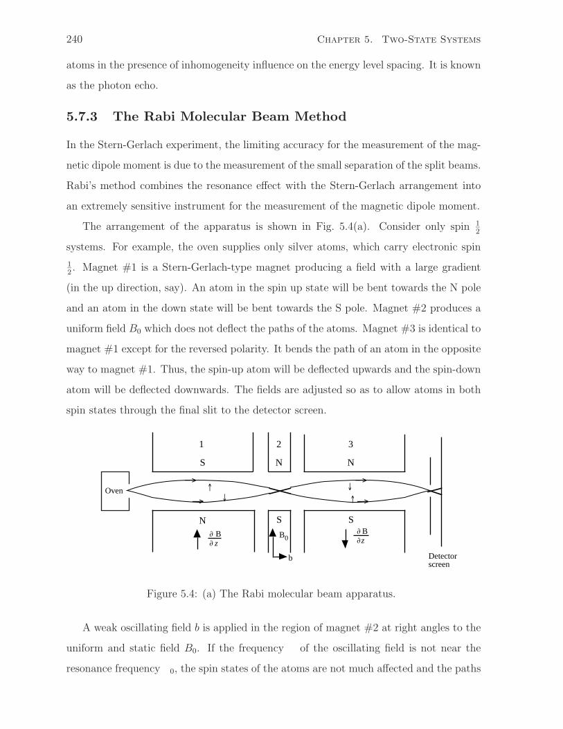
Oven
S
1
N
2
S
N
3
↓↓↑
↑
→
→
→
→
B0
b
N∂∂
Bz
S∂∂
Bz
Detector screen
240 Chapter 5. Two-State Systems
atoms in the presence of inhomogeneity influence on the energy level spacing. It is known
as the photon echo.
5.7.3 The Rabi Molecular Beam Method
In the Stern-Gerlach experiment, the limiting accuracy for the measurement of the mag-
netic dipole moment is due to the measurement of the small separation of the split beams.
Rabi’s method combines the resonance effect with the Stern-Gerlach arrangement into
an extremely sensitive instrument for the measurement of the magnetic dipole moment.
The arrangement of the apparatus is shown in Fig. 5.4(a). Consider only spin 12
systems. For example, the oven supplies only silver atoms, which carry electronic spin
12. Magnet #1 is a Stern-Gerlach-type magnet producing a field with a large gradient
(in the up direction, say). An atom in the spin up state will be bent towards the N pole
and an atom in the down state will be bent towards the S pole. Magnet #2 produces a
uniform field B0 which does not deflect the paths of the atoms. Magnet #3 is identical to
magnet #1 except for the reversed polarity. It bends the path of an atom in the opposite
way to magnet #1. Thus, the spin-up atom will be deflected upwards and the spin-down
atom will be deflected downwards. The fields are adjusted so as to allow atoms in both
spin states through the final slit to the detector screen.
Figure 5.4: (a) The Rabi molecular beam apparatus.
A weak oscillating field b is applied in the region of magnet #2 at right angles to the
uniform and static field B0. If the frequency ω of the oscillating field is not near the
resonance frequency ω0, the spin states of the atoms are not much affected and the paths
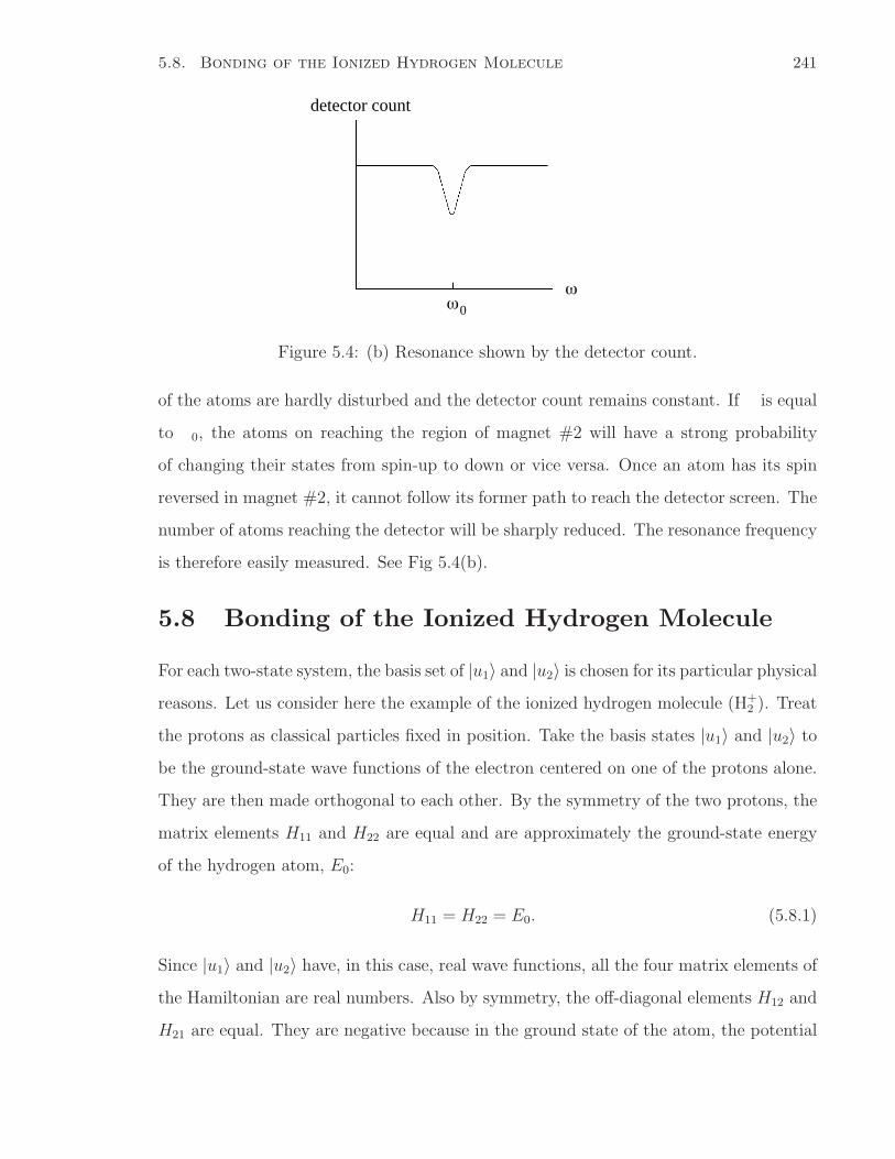
ω
detector count
ω0
5.8. Bonding of the Ionized Hydrogen Molecule 241
Figure 5.4: (b) Resonance shown by the detector count.
of the atoms are hardly disturbed and the detector count remains constant. If ω is equal
to ω0, the atoms on reaching the region of magnet #2 will have a strong probability
of changing their states from spin-up to down or vice versa. Once an atom has its spin
reversed in magnet #2, it cannot follow its former path to reach the detector screen. The
number of atoms reaching the detector will be sharply reduced. The resonance frequency
is therefore easily measured. See Fig 5.4(b).
5.8 Bonding of the Ionized Hydrogen Molecule
For each two-state system, the basis set of |u1〉 and |u2〉 is chosen for its particular physical
reasons. Let us consider here the example of the ionized hydrogen molecule (H+2 ). Treat
the protons as classical particles fixed in position. Take the basis states |u1〉 and |u2〉 to
be the ground-state wave functions of the electron centered on one of the protons alone.
They are then made orthogonal to each other. By the symmetry of the two protons, the
matrix elements H11 and H22 are equal and are approximately the ground-state energy
of the hydrogen atom, E0:
H11 = H22 = E0. (5.8.1)
Since |u1〉 and |u2〉 have, in this case, real wave functions, all the four matrix elements of
the Hamiltonian are real numbers. Also by symmetry, the off-diagonal elements H12 and
H21 are equal. They are negative because in the ground state of the atom, the potential
242 Chapter 5. Two-State Systems
energy overwhelms the kinetic energy. Thus,
H12 = H21 = −V, (5.8.2)
where V is a real and positive number, of the order 1 eV.
5.8.1 The covalent bond
The lower energy state is
|ψ1〉 = 2−1/2(|u1〉 + |u2〉), (5.8.3)
and the energy
E1 = E0 − V. (5.8.4)
The molecule is symmetric about the plane perpendicular bisecting the line joining the
protons. The lower state wave function is of even parity, and is said to be gerade (mostly
by theoretical chemists) which is just the German way of saying symmetric, and which
is usually denoted by a subscript g.
The higher energy state is
|ψ2〉 = 2−1/2(|u1〉 − |u2〉), (5.8.5)
and energy E2 = E0 + V. (5.8.6)
The higher state wave function is of odd parity, and is also said to be ungerade, denoted
by a subscript u.
By sharing the electron between the two protons symmetrically, the system lowers its
energy by an amount of V . Thus, the electron binds the molecule and is said to be in a
bonding state (or orbital). The higher energy state is an antibonding orbital and does
not bind the molecule.
5.8.2 Time evolution of the electron in the bonding state
Suppose that we bring together very quickly a hydrogen atom and a hydrogen ion (i.e., a
proton) to form the molecular ion, such that initially the electron is in the ground state
of one of the protons, say u1. How does the electron state develop in time?
5.8. Bonding of the Ionized Hydrogen Molecule 243
According to the Schrodinger theory, the electron state has the time dependence given
in terms of the energy eigenstates by
Ψ(t) = ψ1c1e−iE1t/h + ψ2c2e
−iE2t/h. (5.8.7)
Initially, i.e., at t = 0, it is given that
Ψ(0) = u1. (5.8.8)
From Eq. (5.8.7) it follows that
c1 = c2 = 2−1/2. (5.8.9)
Hence, in terms of the basis set u1 and u2,
Ψ(t) =1
2[(u1 + u2)e
−i(E0−V )t/h + (u1 − u2)e−i(E0+V )t/h]
= u1e−iE0t/h cos
(V t
h
)
+ u2ie−iE0t/h sin
V t
h. (5.8.10)
The probability of the electron being in state |u1〉, roughly speaking in the atomic
ground state around proton #1, is
P1 = [cos(V t/h)]2. (5.8.11)
Probability of the electron being in state |u2〉, i.e., around proton #2, is
P2 = [sin(V t/h)]2. (5.8.12)
These probabilities are plotted as functions of t in Fig. 5.5. The electron oscillates
between the two protons with frequency ω = 2V/h.
There is a classical analogue of this phenomenon. If two identical tuning forks are
placed on top of a resonance box and one fork is plucked, then the sound energy will slosh
back and forth from one fork to the other. By analogy with this classical phenomenon,
Pauling called the hopping back and forth of the electron from one proton to the other a
“resonance”. Thus, the chemical bond can be described either in the time independent
picture as the splitting of the two states of equal energy E0 into a bonding state with
energy E0 − V and an antibonding state with energy E0 + V due to the overlap of the
atomic wave functions or in the time dependent picture as due to the electron going back
and forth from one ion to another with a resonance frequency 2V/h.
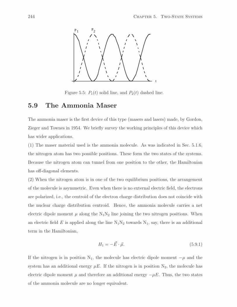
t
P1 P2
244 Chapter 5. Two-State Systems
Figure 5.5: P1(t) solid line, and P2(t) dashed line.
5.9 The Ammonia Maser
The ammonia maser is the first device of this type (masers and lasers) made, by Gordon,
Zieger and Townes in 1954. We briefly survey the working principles of this device which
has wider applications.
(1) The maser material used is the ammonia molecule. As was indicated in Sec. 5.1.6,
the nitrogen atom has two possible positions. These form the two states of the systems.
Because the nitrogen atom can tunnel from one position to the other, the Hamiltonian
has off-diagonal elements.
(2) When the nitrogen atom is in one of the two equilibrium positions, the arrangement
of the molecule is asymmetric. Even when there is no external electric field, the electrons
are polarized, i.e., the centroid of the electron charge distribution does not coincide with
the nuclear charge distribution centroid. Hence, the ammonia molecule carries a net
electric dipole moment µ along the N1N2 line joining the two nitrogen positions. When
an electric field E is applied along the line N1N2 towards N1, say, there is an additional
term in the Hamiltonian,
H1 = − E · µ. (5.9.1)
If the nitrogen is in position N1, the molecule has electric dipole moment −µ and the
system has an additional energy µE. If the nitrogen is in position N2, the molecule has
electric dipole moment µ and therefore an additional energy −µE. Thus, the two states
of the ammonia molecule are no longer equivalent.
5.9. The Ammonia Maser 245
(3) An electrical analogue of the Stern-Gerlach set-up is used to split a beam of ammonia
molecules into two beams one in each of the two energy states described above. The higher
energy state molecules are passed into a microwave cavity. In thermal equilibrium, the
ammonia molecules are distributed between the energy states according to the Boltzmann
law. This process of getting a larger portion into the upper energy level than the thermal
distribution is known as the population inversion.
(4) The excited ammonia molecules in the microwave cavity can lose energy in the form
of a photon (of microwave frequency) either by spontaneous emission or by stimulated
emission which has a probability proportional to the photon distribution of that frequency
already present in the cavity. The cavity serves as a resonator which builds up the number
of photons of the same frequency into a coherent beam of microwave radiation.
The advantages of this device are: (i) An output of narrow frequency range. The
limitation due to the molecule de-excitation process is ∆ω/ω 10−12. (ii) The operation
is very stable, about 1 in 1010 drift over long periods. Thus, an important use of the
maser is as an atomic clock. The deviation from true periodicity is about 1 sec in a
century.
The disadvantages of the ammonia maser are: (i) The frequency is fixed. It is equal
to 2h
√(µE)2 + V 2 which can be changed by adjusting the electric field. (For a way to
define V , see Problem 10). However, the microwave cavity is of fixed dimension and
therefore fixed resonance frequency which is not tunable. (ii) The width of the frequency
distribution ∆ω = 4 kHz is relatively large in this business. (iii) The power output of
10−9 watt is weak.
When the emitted radiation has frequency in the range of light, the device is called a
laser. The operating principles are the same:
(1) Two energy levels are needed. There are, by now, an enormous range of materials. A
common example is ruby which is just Al2O3 with C3+ impurities (substituting aluminum
ions). The electronic states in the chromium ion impurity have three energy levels. The
two upper levels are closer in energy. The highest energy level has a very short life-
time. When the Cr ion is excited from the lowest energy level to the highest energy
level, it relaxes very fast to the middle level where it is de-excited to the lowest level
246 Chapter 5. Two-State Systems
by stimulating emission of photons. Other systems include CO2, YIG, and various dyes.
Dyes have a broad distribution of energy levels being large molecules with lots of closely
spaced electronic energy levels which provide the possibility of tuning (variable frequency
output).
(2) A mechanism for population inversion. More common than the Stern-Gerlach type
arrangement are optical pumping or atom bombardment. For the three level system in
ruby, the excitation from the lowest level to the highest is done by light input with a
higher frequency than the coherent output.
(3) A resonator for stimulated emission is needed. In lasers, the microwave cavity is
replaced by a Fabry-Perot type mirror arrangement to allow the emitted radiation to
oscillate back and forth to build up its intensity.
Lasers have many applications. One of the most fascinating from the point of view of
applying the principles of quantum physics is the separation of isotopes by lasers. Isotopes
of an element differ only by the number of neutrons in the nucleus. They are difficult to
distinguish chemically. The electronic energy levels differ only by minute amounts due to
the difference in the reduced mass. Laser light has such a narrow frequency distribution
that it can excite one isotope without exciting another with a slightly different excitation
energy. The excited atoms have very different magnetic or electric dipole moments from
their isotopic brethren which were not excited by the laser light. The two different
isotopes can then be separated by an inhomogeneous magnetic or electric field as in a
Stern-Gerlach experiment.
5.10 Strangeness Oscillations of the Kaons
To demonstrate the ubiquitous nature of the two-state systems, we now apply it to the
strange particles. To understand how a two-state system may be extracted from a larger
number of mesons, we describe briefly the background in elementary particle physics.
There is a bewildering variety of elementary particles, leading to the quip that all
particles are elementary though some are more elementary than others. They are now
generally classified into four families.
1. Field particles (gauge particle) such as photons, the W± and Z0 particles and the
5.10. Strangeness Oscillations of the Kaons 247
gluons. They are exchanged during the interaction between two particles. For
example, the electromagnetic interaction between two charged particles may be
viewed as exchange of a photon.
2. Leptons: the family of particles which interact with only weak and electromagnetic
interaction includes the electron, neutrino, and µ meson (muon).
3. Hadrons: those interacting with strong interaction. There are two families of such
particles:
(a) Mesons. Particles of integer spins (bosons) which include the pions (π mesons)
and the kaons (K mesons).
(b) Baryons. Particles of integer-plus-half spins (fermions) which include the sta-
ble nucleons. The baryons are distinguished from the mesons by the baryon
number (±1). The assignment of the baryon number explains the occurrence
and non-occurrence of certain decays and reactions since all of them obey
baryon number conservation.
Consider now only the meson family. The kaons and the pions are distinguished
by a property known as the strangeness. The law of conservation of strangeness which
correlates the decay events of the particles stipulates that
1. The total strangeness must remain constant if the processes involve strong or elec-
tromagnetic interaction.
2. The total strangeness may remain constant or change by ±1 if only the weak
interaction (without the electromagnetic interaction) is involved.
For particles with strong interaction (of the order 10 MeV), the decay processes are
expected to take place within 10−22 s by the energy-time uncertainty relation. Yet, some
of these decay processes take place on a much longer time scale of 10−10 s, characteristic
of the weak interaction. The introduction of the additional quantum number called
strangeness to the particles and of the conservation of strangeness in particle reactions by
the strong interaction would then forbid certain decay processes if the weak interaction is
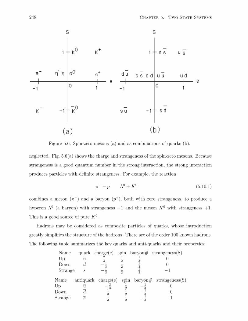
248 Chapter 5. Two-State Systems
Figure 5.6: Spin-zero mesons (a) and as combinations of quarks (b).
neglected. Fig. 5.6(a) shows the charge and strangeness of the spin-zero mesons. Because
strangeness is a good quantum number in the strong interaction, the strong interaction
produces particles with definite strangeness. For example, the reaction
π− + p+ → Λ0 + K0 (5.10.1)
combines a meson (π−) and a baryon (p+), both with zero strangeness, to produce a
hyperon Λ0 (a baryon) with strangeness −1 and the meson K0 with strangeness +1.
This is a good source of pure K0.
Hadrons may be considered as composite particles of quarks, whose introduction
greatly simplifies the structure of the hadrons. There are of the order 100 known hadrons.
The following table summarizes the key quarks and anti-quarks and their properties:
Name quark charge(e) spin baryon# strangeness(S)Up u 2
312
13
0Down d −1
312
13
0Strange s −1
312
13
−1
Name antiquark charge(e) spin baryon# strangeness(S)Up u −2
312
−13
0Down d 1
312
−13
0Strange s 1
312
−13
1
5.10. Strangeness Oscillations of the Kaons 249
Figure 5.6(b) shows the combinations of quarks and antiquarks which would yield
mesons of the same characteristics.
The particles K0 and K 0 have strangeness ±1 and, therefore, by strong interaction
alone which conserves strangeness, cannot convert into each other. However, by weak
interaction, they can convert into each other through their coupling to pions which have
zero strangeness. The two particle states K0 and K 0 can be considered as a two-state
system if the intermediate pion states are eliminated and their influence is replaced by
an effective matrix element of the Hamiltonian connecting the two states, Ah, where A is
real. As we have seen earlier, because of the weak interaction, A is of the order 1010 s−1
and Ah is of the order 10−5 eV. The diagonal matrix element connecting K0 or K 0 to
itself is also Ah if it is also via the same two-pion intermediate state. The Hamiltonian
is
H =
[A AA A
]
h. (5.10.2)
In the diagonal terms of the Hamiltonian we have left out the equal energy (mass) of the
K0 and K 0 particles of 500 MeV, which is enormous compared with the other terms.
The qualitative description of the reduction of the Hamiltonian to the two-state system
given above is illustrated quantitatively in Problem 11.
The energy difference of the two energy eigenstates, the symmetric state being called
K0L and the antisymmetric state K0
S, is 2Ah. It is measured to be 0.5×10¹⁰ hs−1, in good
agreement with the theoretical anticipation of it being “second order” weak interaction.
If the particle is initially a K0 particle, then the probability of it converting to a K 0
at time t is
P (t) = sin2(At). (5.10.3)
This is called the “strangeness oscillations”. The deduction of this result is left as a
problem. If we wish to include phenomenologically the fact that each particle can decay
into something else than the other particle, we replace the real number A by a complex
number A − iΓ, where Γ is positive. Then, the Hamiltonian is not Hermitian and Γ
measures the rate of disappearance of the particle from the two-state system. (See
250 Chapter 5. Two-State Systems
Problem 1.13). The probability of a K0 converting to a K 0 at time t is
P (t) =1
4[1 + e−4Γt − e−2Γt2 cos(2At)]. (5.10.4)
The strangeness oscillations have been observed experimentally by producing a beam
of K0 using the strong-interaction reaction process in Eq. (5.10.1) and monitoring the
intensity of K 0 by measuring the hyperons produced by the strong-interaction reaction
K 0 + p+ → Λ0 + π+ . (5.10.5)
Notice that strangeness is conserved in the reaction because Λ0 and K 0 both have
strangeness −1.
Actually, the two energy eigenstates KL and KS have different decay times, τL ∼10−7 s and τS ∼ 10−10 s. Because of the difference in the CP (charge conjugation and
parity) symmetry, KS can decay into two pions (π+ and π−) but KL can only decay into
three pions, leading to the difference in decay times.
Pais and Piccioni suggested an experiment to observe the mixing of the K0 and K 0
states into KL and KS, known as the K0 regeneration. If a pure K0 beam is allowed to
move in vacuum for a time about 100τS, the constituent state KS will decay, leaving only
a beam of KL. Now pass the beam through a slab of material. The strong interaction
between the K 0 component in KL and protons p in the slab will produce hyperons, as in
Eq. (5.10.5), which can be measured. This was experimentally confirmed a year later by
Fry et al. The regeneration is an illustration of the quantum phenomenon of two-state
mixing, analogous to passing the spin 1/2 particles through a series of Stern-Gerlach
apparati, arranged as in the Problem 16.
Study of the decay of the long-lived kaon KL led to the discovery of the violation of
the CP symmetry. Denote the eigenstates of Eq. (5.10.2) as
|K±〉 =1√2(|K0〉 + |K0〉). (5.10.6)
The states K0 and K0
are related by the CP operation,
CP |K0〉 = |K0〉. (5.10.7)
Then, the mixed states K± are eigenstates of CP with eigenvalues ±1. Above, the K−
and K+ states were identified respectively as the long- and short-lived kaons KL and KS.
5.11. Isospin of nucleons 251
In 1964, Cronin, Fitch, et al. found that the long-lived KL also had a small probability
in decaying into two pions like the short-lived KS. In other words, they are not pure K±:
|KL〉 = |K−〉 + ε|K+〉
|KL〉 = |K+〉 − ε|K−〉. (5.10.8)
where ε ≈ 2×10⁻³. CP violation has serious implications for the particle theory. Intense
pursuit is being conducted to seek additional examples of CP violation. B quarks are
being viewed as another likely candidate.
5.11 Isospin of nucleons
Proton and neutron are regarded as two states of a nucleon. Thus, we can write the two
charge states as the spin-up and down states of the z-component of a pseudo-spin operator
of spin 1/2, know as the isospin, denoted by T , which are dimensionless observables
obeying the same commutation relations as the spin vector but with h removed. This
pseudo-spin vector can be used to construct a representation of the charge property of
the nucleon.
The three components of the isospin vector T are usually denoted by the suffices
(1,2,3) instead of (x,y,z). The proton state and neutron state which are eigenstates of T3
have the vector representation
p =
[10
]
,
n =
[01
]
. (5.11.1)
The charge operator is
Q =e
2(1 + T3) = =
[e 00 0
]
, (5.11.2)
where e is the proton charge. The proton and neutron states are the eigenstates of Q:
Q|p〉 = e|p〉,
Q|n〉 = 0|n〉, (5.11.3)
252 Chapter 5. Two-State Systems
with the correct charges for the eigenvalues.
In nuclear binding, the dominant interaction between the nucleons is much stronger
than the electromagnetic interaction and is referred above as the strong interaction. We
examine the structure of the strong interaction Hamiltonian in the isospin space of one
nucleon and of two nucleons. The Hamiltonian H of a single nucleon is, in the absence
of the electromagnetic interaction, independent of the charge of the nucleon and thus
commutes with Q and T3:
[H, T3] = 0. (5.11.4)
The eigenvalue of H for an energy eigenstate is unchanged if a proton state in it is
changed into a neutron state or vice versa. Thus, H commutes with T+ and T− and,
therefore,
[H, T1] = 0 and [H, T2] = 0. (5.11.5)
Thus, H has a diagonal representation in the isospin space with equal elements in the
diagonal.
For two nucleons, the Hamiltonian is a function of both isospin vectors T (j), j = 1, 2.
Since the Hamiltonian cannot depend on the specific orientation of either one or the other,
it can only depend on their relative orientation. Apart from two single nucleon terms,
the interaction term has the form T (1) · T (2), or equivalently, (T (1) + T (2))2. With these
simple constructions, we can illustrate by problems 14 and 15 a physical understanding
of the nuclear structure of the pr-deuterons and of the series of nuclei, 6He, 6Li, and 6Be.
5.12 Examples
5.12.1 An operator which commutes with the Pauli matrices
An operator has a 2 × 2 matrix representation in the spin 1/2 space, denoted by A. It
commutes with the three components of the Pauli matrices, [A,σ] = 0. Show that A
must a scalar times the unit matrix and give an example for A.
Solution — From Sec. 5.1 or Problem 1, A has the form
A = α0 + α · σ, (5.12.1)
5.12. Examples 253
with four coefficients α0 and α which commute with the Pauli matrices and the unit
matrix multiplying α0 understood. Thus,
[A, σx] = [α0 + α · σ, σx]
= αy[σy, σx] + αz[σz, σx]
= −2iαyσz + 2iαzσy, (5.12.2)
whose vanishing leads to the zero coefficients:
αy = 0,
αz = 0. (5.12.3)
Similarly, commutation brackets with the other components lead to the additional
αx = 0. (5.12.4)
Therefore, A is α0 times the unit matrix. An example is S2, which is 34
times the unit
matrix.
5.12.2 Neutron spin precession
In the experimental setup illustrated by Fig. 5.7, a beam of neutrons along the y direction
is polarized (how?) to have all the spins lined up in the positive x direction. The neutrons
then travel through a uniform magnetic field B pointing in the z direction and enter a
detector at a distance L, which can be varied. The detector measures the neutron spin
in the x direction.
(a) As the distance L between the detector and the polarizer is varied, the measured
spin in the x direction will vary sinusoidally. Find the change in the distance ∆L
which corresponds to one period of change in the measured spin in terms of the
magnetic field B and the neutron wavelength λ.
Solution — The neutron speed is
v =h
λmN
, (5.12.5)
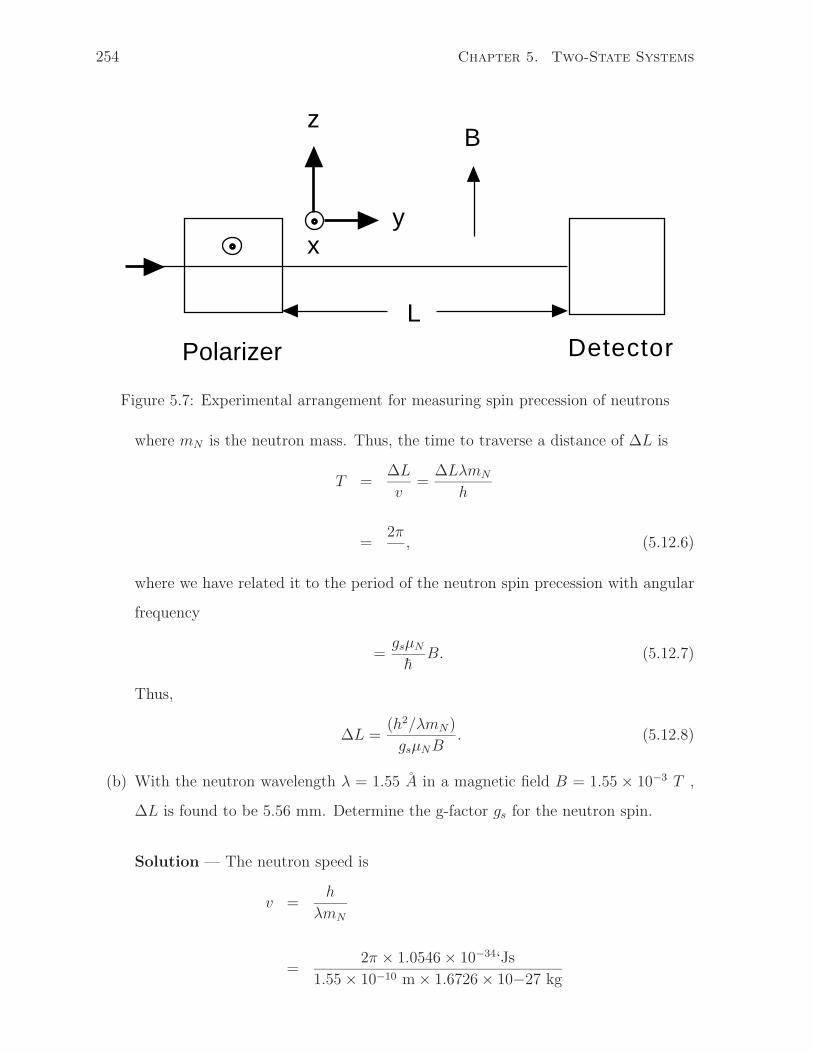
xy
z
Polarizer DetectorL
B
254 Chapter 5. Two-State Systems
Figure 5.7: Experimental arrangement for measuring spin precession of neutrons
where mN is the neutron mass. Thus, the time to traverse a distance of ∆L is
T =∆L
v=
∆LλmN
h
=2π
ω, (5.12.6)
where we have related it to the period of the neutron spin precession with angular
frequency
ω =gsµN
hB. (5.12.7)
Thus,
∆L =(h2/λmN)
gsµNB. (5.12.8)
(b) With the neutron wavelength λ = 1.55 A in a magnetic field B = 1.55 × 10⁻³ T ,
∆L is found to be 5.56 mm. Determine the g-factor gs for the neutron spin.
Solution — The neutron speed is
v =h
λmN
=2π × 1.0546 × 10−34‘Js
1.55 × 10−10 m × 1.6726 × 10−27 kg
5.12. Examples 255
= 2.556 × 10³ m/s , (5.12.9)
so that the frequency is
1
T=
v
∆L= 4.601 × 10⁴ Hz (5.12.10)
corresponding to an energy of
h
T= 1.904 × 10⁻⁷ meV. (5.12.11)
The energy corresponding to the resonance frequency is
gsµNB = gs 3.1525 × 10⁻⁵ meV/T × 1.55 × 10⁻³ T
= gs 4.886 × 10⁻⁸ meV. (5.12.12)
Equating the two energies yields the g-factor
gs = 3.90 (5.12.13)
which is quite close to the accepted value.
5.12.3 An application of the transformation matrix
A beam of particles of spin 12
is sent through a Stern-Gerlach apparatus. One of the
resulting beams is sent through another similar apparatus with the magnetic field at an
angle α with respect to that of the first apparatus. What are the relative numbers of
particles that appear in the two beams leaving the second apparatus?
Solution — Let the magnetic field in the first Stern-Gerlach apparatus be along the
z-axis and the particle beam be along the y-axis. The corresponding directions in the
second apparatus will be denoted by the z’-axis and y’-axis respectively. The new axes
are obtained from the old ones by rotation through an angle α about the y-axis. Thus,
y and y’ axes are the same. The spin-up and down states along the z’-axis are related to
those along the z-axis by Eq. (5.2.6):
[ψ+ ψ−] = [χ+ χ−]
[cos α
2− sin α
2
sin α2
cos α2
]
, (5.12.14)
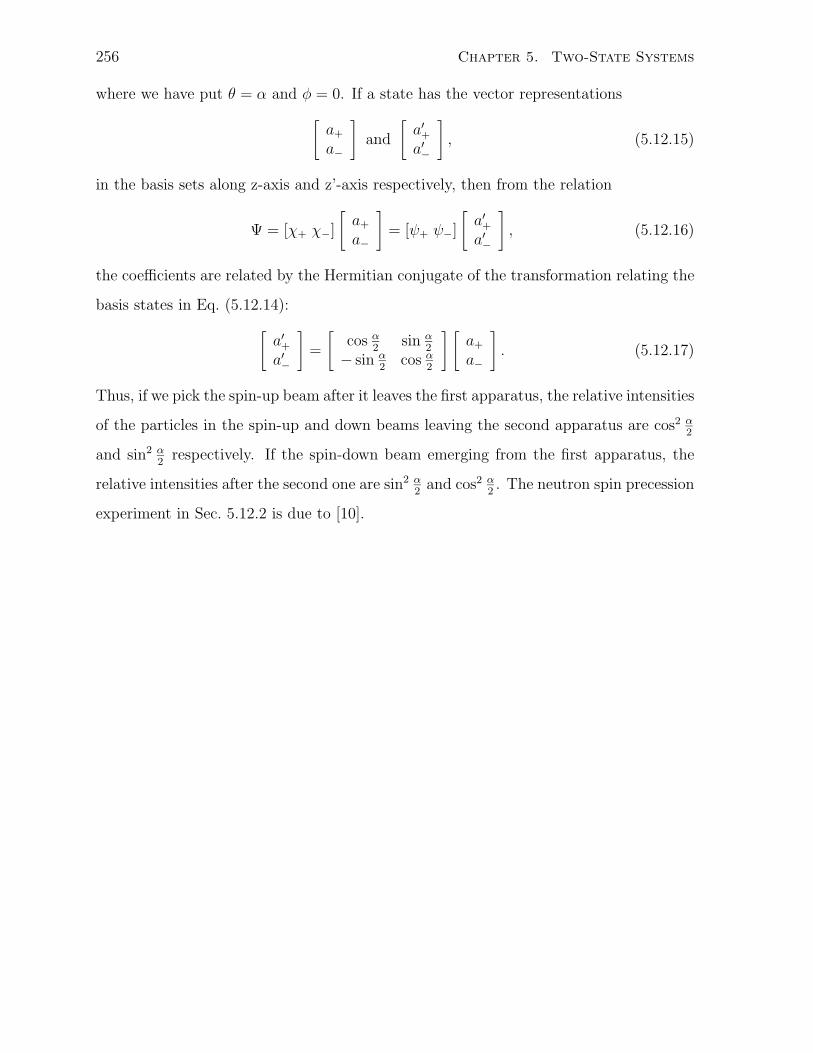
256 Chapter 5. Two-State Systems
where we have put θ = α and φ = 0. If a state has the vector representations
[a+
a−
]
and
[a′
+
a′−
]
, (5.12.15)
in the basis sets along z-axis and z’-axis respectively, then from the relation
Ψ = [χ+ χ−]
[a+
a−
]
= [ψ+ ψ−]
[a′
+
a′−
]
, (5.12.16)
the coefficients are related by the Hermitian conjugate of the transformation relating the
basis states in Eq. (5.12.14):
[a′
+
a′−
]
=
[cos α
2sin α
2
− sin α2
cos α2
] [a+
a−
]
. (5.12.17)
Thus, if we pick the spin-up beam after it leaves the first apparatus, the relative intensities
of the particles in the spin-up and down beams leaving the second apparatus are cos2 α2
and sin2 α2
respectively. If the spin-down beam emerging from the first apparatus, the
relative intensities after the second one are sin2 α2
and cos2 α2. The neutron spin precession
experiment in Sec. 5.12.2 is due to [10].
5.13. Problems 257
5.13 Problems
1. Properties of Pauli Matrices
Prove the essential properties of the Pauli matrices and a useful identity:
(a) Any 2 × 2 matrix A (which does not have to be Hermitian) can be expressed
as A = α0 1 + α · σ. Find α0 and α in terms of the matrix elements of A.
(b) σxσy = −σyσx = iσz, etc.
(c) σ2x = 1, etc.
(d) For any two vectors of operators A and B which commute with σ,
( A · σ)( B · σ) = A · B + i( A × B) · σ. (5.13.1)
2. By diagonalizing the Pauli matrices σx and σy, find the spin up and down states in
the x and y directions in terms of the basis set of the eigenstates of σz.
3. Density matrix of two-level systems
(a) Find the density matrix for an ensemble of spin-1/2 systems with a fraction
12
+ p in the spin-up states along the (θ, φ) direction and a fraction 12− p in
the spin-down states.
(b) Relate the density matrix elements to the coefficients a0, ax, ay, az of the form
ρ = a0I + a · σ, (5.13.2)
and, hence, show that the ensemble average of the spin S completely deter-
mines the density matrix of an ensemble of spin 1/2 particles.
(c) Show that an unpolarized ensemble (half in spin-up and half in spin-down
states along a chosen direction) remains unpolarized in any direction.
(d) All the spins of an ensemble of spin-1/2 particles point in the plane bisecting
the angle between the zx and yz plane. The probability distribution of the
angle θ of the spin state about the z axis is proportional to sin θ. Is this a
coherent ensemble?
258 Chapter 5. Two-State Systems
4. The Bloch Equations with dissipation
(a) For a time-dependent field b perturbing a conservative Hamiltonian system of
spin 12, establish the equation of motion for the expectation values for the spin
vector in the form
d
dt〈S〉 = γ〈S〉 × B.
Find an expression for γ, know as the gyromagnetic ratio. This equation is
valid for any spin, not just spin 1/2.
(b) Let the total magnetic field be in the form B = (b cos ωt, b sin ωt, B0), where b,
ω, and B0 are constants. Deduce from the Lindblad form of the master equa-
tion the dissipative terms for the Bloch equation in terms of the longitudinal
relaxation time T1 and the transverse relaxation time T2.
5. Transverse magnetic susceptibility. Obtain from the Bloch equations in Prob-
lem 4 the magnetization (or the polarization) to first order in the transverse mag-
netic field b as a function of the resonance frequency.
6. Spin Precession via the Bloch equations
Another way of demonstrating spin precession in a magnetic field. Let the static
magnetic field B be along the z-direction. A spin 12
particle with a magnetic dipole
moment µ is initially in a state with expectation values of the spin (mx, 0, mz).
(a) From the Bloch equations neglecting the damping terms, show that the ex-
pectation values of the spin at time t is given by,
〈Sx〉 = mx cos(ωt),
〈Sy〉 = mx sin(ωt),
〈Sz〉 = mz.
Find ω, the magnetic resonance frequency in relation to the energy eigenstates
of the spin in the magnetic field.
5.13. Problems 259
(b) Find the effect of the damping terms on the precession.
7. Rabi rotation The aim of this problem is to establish explicitly the rotational
operation from the time evolution of the Rabi oscillation. Take the Hamiltonian
given by Eqs. (5.5.3,5.5.4). Assume the relaxation times to be infinitely long.
(a) By the unitary transform of the spin state |Ψ〉 = T |Φ〉, where
T =
[e−iωt 0
0 eiωt
]
, (5.13.3)
show that |Φ〉 obeys the Schrodinger equation with an effective Hamiltonian
which is time independent. Hence, find its time evolution operator as a rota-
tion operator, identifying the rotational axis and the angle of rotation.
(b) Find the corresponding rotation of the spin polarization vector derived from
the density matrix in this “rotational frame”.
(c) Hence, derive the rotations explained in Secs. 5.7.1 and 5.7.2.
8. A particle is initially in the ground state of a potential well W1.
(a) If a second identical well W2 is placed close to W1 for a long time, the energy
separation between the two lowest states in the double well is 2V . Find the
relevant Hamiltonian for the double well.
(b) Now suppose the wells are initially well separated. The well W2 is brought up
suddenly close to W1. The object of the experiment is to capture the particle
in W2 by suddenly removing W1. Calculate the best time of removal.
9. The two-level atom model. The system consists of the (100) and (210) states
of the hydrogen atom. It is driven by an external oscillating electric field E cos(ωt)
along the z direction.
(a) Construct the Hamiltonian matrix of the two-level system. Take the perturb-
ing Hamiltonian to be H1 = −µ · E , where µ = −er is the electron dipole
moment.
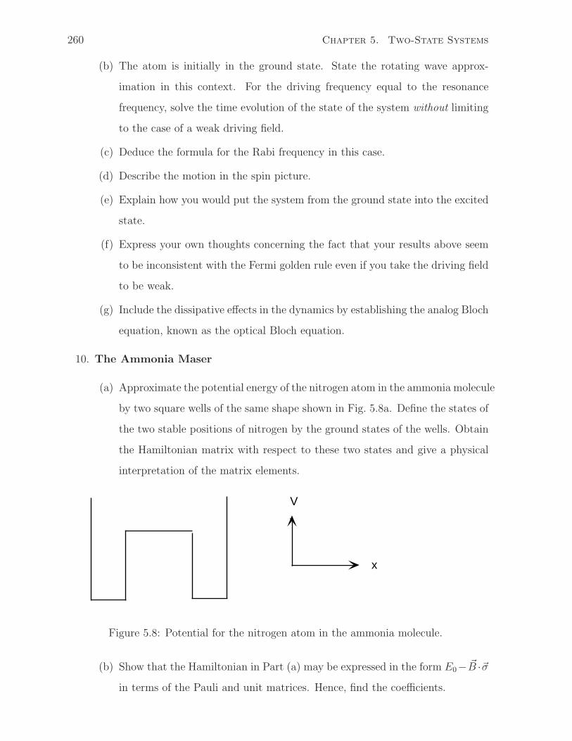
V
x
260 Chapter 5. Two-State Systems
(b) The atom is initially in the ground state. State the rotating wave approx-
imation in this context. For the driving frequency equal to the resonance
frequency, solve the time evolution of the state of the system without limiting
to the case of a weak driving field.
(c) Deduce the formula for the Rabi frequency in this case.
(d) Describe the motion in the spin picture.
(e) Explain how you would put the system from the ground state into the excited
state.
(f) Express your own thoughts concerning the fact that your results above seem
to be inconsistent with the Fermi golden rule even if you take the driving field
to be weak.
(g) Include the dissipative effects in the dynamics by establishing the analog Bloch
equation, known as the optical Bloch equation.
10. The Ammonia Maser
(a) Approximate the potential energy of the nitrogen atom in the ammonia molecule
by two square wells of the same shape shown in Fig. 5.8a. Define the states of
the two stable positions of nitrogen by the ground states of the wells. Obtain
the Hamiltonian matrix with respect to these two states and give a physical
interpretation of the matrix elements.
Figure 5.8: Potential for the nitrogen atom in the ammonia molecule.
(b) Show that the Hamiltonian in Part (a) may be expressed in the form E0− B ·σin terms of the Pauli and unit matrices. Hence, find the coefficients.
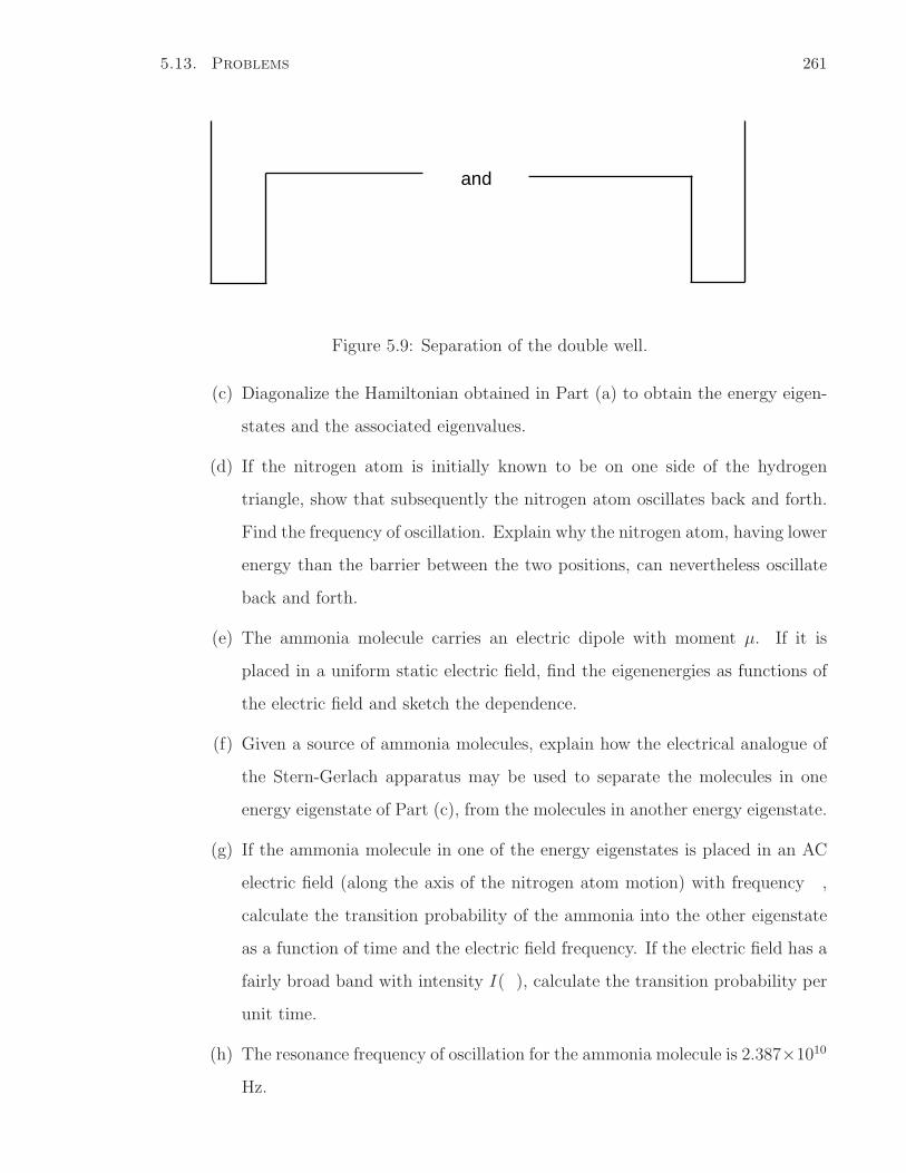
and
5.13. Problems 261
Figure 5.9: Separation of the double well.
(c) Diagonalize the Hamiltonian obtained in Part (a) to obtain the energy eigen-
states and the associated eigenvalues.
(d) If the nitrogen atom is initially known to be on one side of the hydrogen
triangle, show that subsequently the nitrogen atom oscillates back and forth.
Find the frequency of oscillation. Explain why the nitrogen atom, having lower
energy than the barrier between the two positions, can nevertheless oscillate
back and forth.
(e) The ammonia molecule carries an electric dipole with moment µ. If it is
placed in a uniform static electric field, find the eigenenergies as functions of
the electric field and sketch the dependence.
(f) Given a source of ammonia molecules, explain how the electrical analogue of
the Stern-Gerlach apparatus may be used to separate the molecules in one
energy eigenstate of Part (c), from the molecules in another energy eigenstate.
(g) If the ammonia molecule in one of the energy eigenstates is placed in an AC
electric field (along the axis of the nitrogen atom motion) with frequency ω,
calculate the transition probability of the ammonia into the other eigenstate
as a function of time and the electric field frequency. If the electric field has a
fairly broad band with intensity I(ω), calculate the transition probability per
unit time.
(h) The resonance frequency of oscillation for the ammonia molecule is 2.387×10¹⁰
Hz.
262 Chapter 5. Two-State Systems
i. Calculate the off-diagonal Hamiltonian matrix element in electron volts.
ii. Is it also possible to find the diagonal element? Does it matter to the
operation of the ammonia maser?
iii. Estimate the size of the microwave cavity used as a resonator for the
ammonia molecules.
iv. If the operating time of the microwave cavity is about 10−3 seconds, what
is the line-width (full width at half maximum in percentage frequency) of
the ammonia molecule power output?
11. The effective Hamiltonian of the neutral kaons. Take as the basis states the
states of strangeness 1, 0, and −1 for K0, one of the neutral particles with S = 0
in Fig. 5.6, and K0, respectively. The Hamiltonian may be taken in the form,
H =
K W 0W K + ∆ W0 W K
. (5.13.4)
The diagonal terms represent the strong and electromagnetic interactions yield-
ing K the masses of the two neutral kaons and ∆ the mass difference with the
intermediate particle. The off-diagonal terms W represent the weak interaction
(not including the electromagnetic terms). To second order in the small parame-
ter η = W/∆, find a unitary transformation leading to the effective Hamiltonian,
Eq. (5.10.2).
12. The neutral kaon oscillations
(a) Justify on phenomenological ground the introduction of damping in the effec-
tive Hamiltonian Eq. (5.10.2) by replacing A with A− iΓ. Does the resulting
equation fit the Lindblad form?
(b) Deduce Eq. (5.10.3) and (5.10.4).
(c) Find also the probability of the particle remaining a K0 at time t in each case.
13. Photon polarization
Later in the course, we shall quantize the electromagnetic field into photons. Here is
a warm-up exercise on the polarization of the photon. To construct the polarization
5.13. Problems 263
states of a photon, we adopt the following rules of correspondence:
Rule 1: Take the propagation direction of the corresponding classical electric field
along the z axis. For the linearly polarized light along the x axis and along
the y-axis given, respectively, by
E = xE[ei(kz−ωt)], (5.13.5)
E = yE[ei(kz−ωt)], (5.13.6)
where x denotes the unit vector along the x direction, the time-independent
quantum polarization states of the photon corresponding to the above fields
are denoted by |0, z〉 and |π/2, z〉. Use these two states as the basis set.
Rule 2: The quantum state corresponding to the phase-shifted classical field
E = xE[ei(kz−ωt−θ)], (5.13.7)
is given by e−iθ|0, z〉.
(Baym [2] uses the polarization states of the classical electromagnetic field to build
up the quantum theory for two states.)
(a) Find the quantum state |φ, z〉 of the photon propagating along the z axis and
linearly polarized along a vector in the xy-plane at an angle φ from the x-axis
(with the phase θ = 0).
(b) Under the rotation operator R(α, z), the state |φ, z〉 is moved to
R(α, z)|φ, z〉 = |φ + α, z〉. (5.13.8)
Let the generator Gz of the rotation operator be given by
R(δα, z) = 1 − iδαGz + O((δα)2). (5.13.9)
Find the matrix representation of Gz in the basis set of |0, z〉 and |π/2, z〉.
(c) Find the eigenstates of Gz and deduce their physical meaning using the rules
given above.
264 Chapter 5. Two-State Systems
(d) Let |εj〉, j = x, y, z be three linearly polarized states along the Cartesian axes.
Define the three generators Gj as in Eq. (5.13.9). Show that
Sj|εj〉 = iεjk|ε〉, (5.13.10)
where the summation over the repeated index is understood. (See a similar
operator defined in Ref. [16], p. 72.) Show that the components of G satisfy
the commutation relations of the angular momentum vector
[Gi, Gj] = iεijkGk. (5.13.11)
From two of the eigenstates of Gz and G2, argue that the photon has spin 1.
(e) Find the third eigenstate of Gz and G2 and discuss its physical meaning if any.
(f) Even though the photon has two polarization states, why is it not a spin-1/2
Fermion?
14. Stability of a nucleus with two nucleons
The interaction which binds the nucleons, including protons and neutrons, is called
the strong interaction, which is much stronger than the electromagnetic interaction.
The two charge states of a nucleon may be simulated by using the analogous spin
1/2 states, called the isospin, T . The 3-component of the isospin, T3, (analogous
to Sz) has two eigenstates, isospin-up state assigned by convention to proton and
isospin-down state to neutron. (See Sec. 5.11). Now consider a nucleus with two
nucleons. By neglecting the weaker electromagnetic interaction, we expect that the
energy of the nucleus to depend on the magnitude of the sum of the two isospins
(characterized by the quantum number u) but not on the quantum number of the
3-component of the total isospin. In fact, the u = 0 state is bound and the u = 1
states are unbound. Hence, explain (a) why the stable two-particle nucleus must
be composed of a proton and a neutron, (b) why a two-proton or two-neutron
nucleus is always unstable (a stable helium atom contains two protons and one or
two neutrons), (c) why a proton-neutron pair may be unstable and how this state
is different from the stable nucleus in (a).
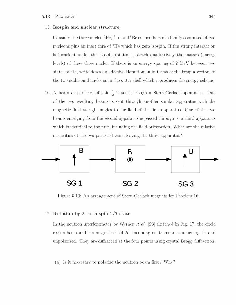
B B B
SG 1 SG 2 SG 3
5.13. Problems 265
15. Isospin and nuclear structure
Consider the three nuclei, 6He, 6Li, and 6Be as members of a family composed of two
nucleons plus an inert core of 4He which has zero isospin. If the strong interaction
is invariant under the isospin rotations, sketch qualitatively the masses (energy
levels) of these three nuclei. If there is an energy spacing of 2 MeV between two
states of 6Li, write down an effective Hamiltonian in terms of the isospin vectors of
the two additional nucleons in the outer shell which reproduces the energy scheme.
16. A beam of particles of spin 12
is sent through a Stern-Gerlach apparatus. One
of the two resulting beams is sent through another similar apparatus with the
magnetic field at right angles to the field of the first apparatus. One of the two
beams emerging from the second apparatus is passed through to a third apparatus
which is identical to the first, including the field orientation. What are the relative
intensities of the two particle beams leaving the third apparatus?
Figure 5.10: An arrangement of Stern-Gerlach magnets for Problem 16.
17. Rotation by 2π of a spin-1/2 state
In the neutron interferometer by Werner et al. [23] sketched in Fig. 17, the circle
region has a uniform magnetic field B. Incoming neutrons are monoenergetic and
unpolarized. They are diffracted at the four points using crystal Bragg diffraction.
(a) Is it necessary to polarize the neutron beam first? Why?
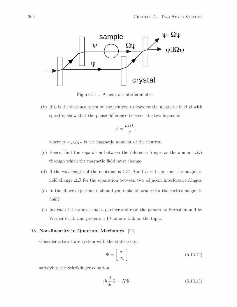
ψ
ψ Ωψ
ψ−Ωψ
ψ+Ωψ
crystal
sample
266 Chapter 5. Two-State Systems
Figure 5.11: A neutron interferometer.
(b) If L is the distance taken by the neutron to traverse the magnetic field B with
speed v, show that the phase difference between the two beams is
φ =µBL
v,
where µ = µNgN is the magnetic moment of the neutron.
(c) Hence, find the separation between the inference fringes as the amount ∆B
through which the magnetic field must change.
(d) If the wavelength of the neutrons is 1.55 Aand L = 1 cm, find the magnetic
field change ∆B for the separation between two adjacent interference fringes.
(e) In the above experiment, should you make allowance for the earth’s magnetic
field?
(f) Instead of the above, find a partner and read the papers by Bernstein and by
Werner et al. and prepare a 10-minute talk on the topic.
18. Non-linearity in Quantum Mechanics. [22]
Consider a two-state system with the state vector
Ψ =
[a1
a2
]
(5.13.12)
satisfying the Schrodinger equation
ihd
dtΨ = HΨ, (5.13.13)
5.13. Problems 267
where the Hamiltonian is given by
H =
[E1 − λ
2f 2
2 00 E2 − λ
2f 2
2 + λf2
]
(5.13.14)
containing a small non-linear term with λ E2 − E1 dependent on the fractional
occupation of the [01
]
state, f2, given by
f2 =|a2|2
|a1|2 + |a2|2. (5.13.15)
(a) Show that homogeneity is preserved, i.e., if Ψ is a solution of the Schrodinger
equation, so is any constant times Ψ.
(b) Show that H is time independent.
(c) Find the wave function at time t given that at t = 0,
Ψ =
[ √1 − b2
b
]
, (5.13.16)
b being a constant.
Describe the relation of Ψ to the eigenstates of the Hamiltonian with no non-
linear terms (λ = 0).
(d) If the system is initially at the lower energy state E1, (i.e., b = 0) and a broad-
band electromagnetic wave is used to excite the system, describe what would
happen to the resonance frequency for absorption.
(e) Describe briefly how you would design an experiment to measure the size of
the non-linear term.
268 Chapter 5. Two-State Systems
5.14 Source Material and Further Reading
This chapter was inspired by the elegant introduction to quantum mechanics by Feynman
[5]. Books which I have consulted for examples of the two-state systems include spin
dynamics [19], isospins [7], quantum optics [1, 4, 11, 18, 21], the covalent bond [14], They
would provide good reading for further study.
The kinetc energy of spin 1/2 particle is due to van der Waerden [20, 17]. For a
discussion of the relation between the Fermi golden rule and the Rabi oscillation, see
Ref. [4], p. 10 or [11], p. 356. An elementary account of the theory and experiment
of the polarization of light to illustrate quantum theory in the beautifully off-beat but
informative book [9]. The polarization of light has also been used by Baym [2] to construct
the quantum theory of the two-state system. The first maser paper is [6]. For many
interesting details in isotope separation, refer to the article [24]. The neutron experiment
used in Problem 17 is carried out by Werner et al. [23] and described in a popular
account in Ref. [3]. The kaon oscillations was originally suggested by Pais and Piccioni
[12]. Readable accounts of the kaons can be found in [5, 8, 15] and CP violation in [7],
Bibliography
[1] L. Allen and J.H. Eberly, Optical Resonance and Two-Level Atoms, (Dover, New
York, 1987).
[2] G. Baym, Lectures on quantum mechanics, (Addison-Wesley, Redwood City,
[3] Herbert J. Bernstein, Scientific Research, August 18, (1969) p. 32.
[4] C. Cohen-Tannoudji, J. Dupont-Roc, and G. Grynberg, Atom-Photon Interactions
– Basic Processes and Applications, (Wiley, New York, 1992).
[5] R.P. Feynman, R.B. Leighton, and M. Sands, The Feynman Lectures on Physics,
Vol. III, (Addison-Wesley, Reading, Mass., 1965) Chapters 6-11.
[6] J.P. Gordon, H.J. Zeiger, and C.H. Townes, Phys. Rev. 95, 282 (1954).
[7] F. Halzen and A.D. Martin, Quarks and Leptons: An Introductory Course in Modern
Particle Physics (J. Wiley, New York, 1984).
[8] K.S. Krane, Introductory Nuclear Physics, (Wiley, New York, 1987).
[9] J-M. Levy-Leblond and F. Balibar, Quantics (North-Holland, Amsterdam 1989).
[10] F. Mesei, Zeit. Phys. 225, 146 (1972).
[11] P. Meystre and M. Sargent III, Elements of Quantum Optics, (Springer, Berlin,
1990).
[12] A. Pais and O. Piccioni, Phys. Rev. 100, 1487 (1955).
[13] Particle Data Group, Phys. Letters B 239, VII 84 (1990).
269
270 BIBLIOGRAPHY
[14] L. Pauling, The Nature of the Chemical Bond (Cornell University Press, New York,
1960).
[15] D.H. Perkins, Introduction to High Energy Physics, (Addison-Wesley, New York,
1972), p. 168 et seq.
[16] J.J. Sakurai, Advanced Quantum Mechanics, (Addison-Wesley, Reading, 1967).
[17] S.S. Schweber, An Introduction to Relativistic Quantum Field Theory (Harper and
Row, New York, 1961), p. 79.
[18] M.O. Scully and M.S. Zubairy, Quantum Optics, (Cambridge University Press, Cam-
bridge 1997).
[19] C.P. Slichter, Principles of Magnetic Resonance, third edition (Springer-Verlag,
Berlin, 1996).
[20] B. L. van der Waerden, Group Theory and Quantum Mechanics, (Springer-Verlag,
Berlin, 1974).
[21] D.F. Walls and G.J. Milburn, Quantum Optics, (Springer, Berlin, 1994).
[22] S. Weinberg, Phys. Rev. Lett 62, 485 (1989); J.J. Bolinger, D.J. Heinzen, W.M.
Itano, S.L. Gilbert, and D.J. Wineland, Phys. Rev. Lett 63, 1031 (1989).
[23] S.A. Werner, R. Colella, A.W. Overhauser, and C.F. Eagen, Phys. Rev. Lett. 35,
1053 (1975).
[24] R.N. Zare in Scientific American, February 1977, p. 86. Calif., 1990).
Chapter 6 Contents
6 Quantum Reality, Information and Computation 2716.1 Introduction . . . . . . . . . . . . . . . . . . . . . . . . . . . . . . . . . . 2716.2 The EPR Paradox and Bell’s Inequalities . . . . . . . . . . . . . . . . . . 272
6.2.1 Measurement of the Two-Spin System . . . . . . . . . . . . . . . 2736.2.2 EPR Paradox and Einstein’s Locality Hypothesis . . . . . . . . . 2756.2.3 Bell’s Inequalities . . . . . . . . . . . . . . . . . . . . . . . . . . . 276
6.3 Rudiments of Quantum Information . . . . . . . . . . . . . . . . . . . . . 2786.3.1 Quantum Cryptography . . . . . . . . . . . . . . . . . . . . . . . 2786.3.2 A Qubit . . . . . . . . . . . . . . . . . . . . . . . . . . . . . . . . 2796.3.3 Entangled States and Quantum Operations . . . . . . . . . . . . . 2796.3.4 Beam me up, Scottie! . . . . . . . . . . . . . . . . . . . . . . . . . 2826.3.5 You’ve Got Mail . . . . . . . . . . . . . . . . . . . . . . . . . . . 284
6.4 A Brief Introduction to Quantum Computation . . . . . . . . . . . . . . 2856.4.1 The Deutsch-Josza algorithm . . . . . . . . . . . . . . . . . . . . 2866.4.2 Requirements for quantum computation . . . . . . . . . . . . . . 287
6.5 Decoherence . . . . . . . . . . . . . . . . . . . . . . . . . . . . . . . . . . 2896.5.1 Dephasing and decoherence . . . . . . . . . . . . . . . . . . . . . 2896.5.2 A demonstration of decoherence . . . . . . . . . . . . . . . . . . . 291
6.6 Problems . . . . . . . . . . . . . . . . . . . . . . . . . . . . . . . . . . . . 2946.7 Source Material and Further Reading . . . . . . . . . . . . . . . . . . . . 298

Chapter 6 List of Figures
6.1 Quantum circuit elements: (a) The Hadamard transform on a single qubit.(b) Controlled-NOT operation on two qubits, where m, n = ±1. (c) Inorder from left to right is the Hadamard transformation followed by C-NOT.281
6.2 A quantum circuit for teleportation (after Fig. 1.13 of Ref. [24] ). . . . . 283

iv
Chapter 6
Quantum Reality, Information andComputation
Cyber space, unlike real space, is not bound by physical concepts.— John H. Minan, Professor of Law,
Opinion Page, San Diego Union, November 25, 1999.
Information is physical!— Rolf Landauer, Physics Letters A 217, 188 (1996).
6.1 Introduction
For a complete quantum theory, it is not sufficient to calculate the wave function of the
state and the eigen-properties of the physical observables using the rules of quantum
mechanics. The theoretical results have to be correctly correlated with the output of
the experimental measurements. This stems from the nature of the measurement of a
quantum system. A measurement causes an abrupt change of a microscopic system to a
pure eigenstate, according to von Neumann’s postulates. These postulates are adopted
because so far no experiments have been found to contradict them. They are necessary
because the alternate of using the microscopic theory including dissipative dynamics of
the macroscopic measurement instrument in each case involves prohibitive labor. This
chapter deals with some salient features of the theory of the measurement processes,
namely the description of the consequences of measurement on the system as well on the
macroscopic measuring system. This part of the theory is formally known as the inter-
pretation of quantum mechanics. In the vast majority of the measurements of quantum
systems, the properties are averaged over a macroscopic ensemble or the measurement
is a one-shot affair. And so following the von Neumann postulates and interpreting the
271
272 Chapter 6. Quantum Reality, Information and Computation
results in terms of probabilities of the eigenstates is adequate. However in the last two
decades or so, the rapid advances of the measuring techniques and of the preparation
of microscopic and mesoscopic (in size somewhere between microscopic and macroscopic
systems) have made it possible to examine the microscopic properties more directly and
to repeatedly measure the microscopic system. This means that the dynamics of the
microscopic system has to be followed including intrusions of the measuring instrument.
A basic knowledge of the measurement theory becomes an essential part of the quantum
theory.
The most far reaching fundamental issues are brought out by two famous problems,
the so called EPR paradox, put forward by A. Einstein, B. Podolsky and N. Rosen and
the life and death of Schrodinger’s cat. We shall study not only the posed problem but
also the resolution: in the EPR case, the Bell theorem and associated experiments and
in the Schrodinger’s cat problem, the phenomenon of decoherence.
Remarkable advances were made recently in the theory of information processing
and computation based on quantum dynamics of the information coded in quantum
systems. Quantum information processing and computation are expected and shown in
theory to supersede the classical ways currently employed in a number of interesting
cases. Although the electronic processes in a transistor are quantum in nature, the
binary number coded depends on two values of the voltage built upon the charge of a
large number of electrons without regard to their quantum properties. Thus, the extant
computation processes are based on the concepts of classical physics. The theory effort in
quantum information and computation has stimulated blossoming research programs for
the physical realization of such quantum devices. Since consideration of such applications
may depend crucially on a thorough understanding of the consequences of quantum
theory, it is educational to examine some of the basic notions here.
6.2 The EPR Paradox and Bell’s Inequalities
EPR stands for A. Einstein, B. Podolsky and N. Rosen who questioned whether quantum
theory was a complete description of physical reality. J. S. Bell found that the paradox
posed by the EPR definition of physical reality against quantum theory could be formu-
6.2. The EPR Paradox and Bell’s Inequalities 273
lated as a set of inequalities of measured quantities subjected to experimental testing.
Experiments have shown that the results are consistent with quantum theory and not
with the Einstein’s requirement of physical reality. (See, for example, ). D. Bohm [5]
changed the EPR illustrative example of a two-particle system to a two-spin system.
Following the chapter on the two-state systems, this then serves very well as a vehicle
for us to delve a little deeper into the predictions of quantum theory.
6.2.1 Measurement of the Two-Spin System
In Chapter 4, we have worked out the eigenstates of the total spin in a system of two
spin-1/2 particles. For example, the singlet state with zero total momentum and zero
z-component is given by
|Ψ0,0〉 =
√1
2(| + z,−z〉 − | − z, +z〉), (6.2.1)
where we have used the first ±z to denote the spin-up and down states along the z-axis
of the first particle and the second placed ±z to denote the states of the second particle.
This state is an example of an entangled states, that is, while it is the sum of products of
states of two (for example) particles which cannot be expressed as a product of a state of
one particle times another state of the second. If the spin of the first particle is measured
along the z direction after the composite is prepared in the singlet state, then we know
for certain the outcome of a subsequent measurement of the spin of the second particle
along the z axis. For example, if the result of measuring the first leads to the spin-up
state, then the system has collapsed to the state | + z,−z〉 and the second particle is
definitely in the spin-down state. If we rotate the axis of measurement to the x-direction,
since the singlet state must be isotropic, i.e., independent of the axis direction,
|Ψ0,0〉 =
√1
2(| + x,−x〉 − | − x, +x〉). (6.2.2)
We can verify this direction by the transformation for each spin:
| + z〉 =
√1
2(| + x〉 − | − x〉). (6.2.3)
Again a measurement of the first spin along the x direction leads to the second particle
being in a definite spin direction along x. However, if a measurement of Sz is now made
on the second, there would be only a fifty-fifty chance of finding the spin-up state.
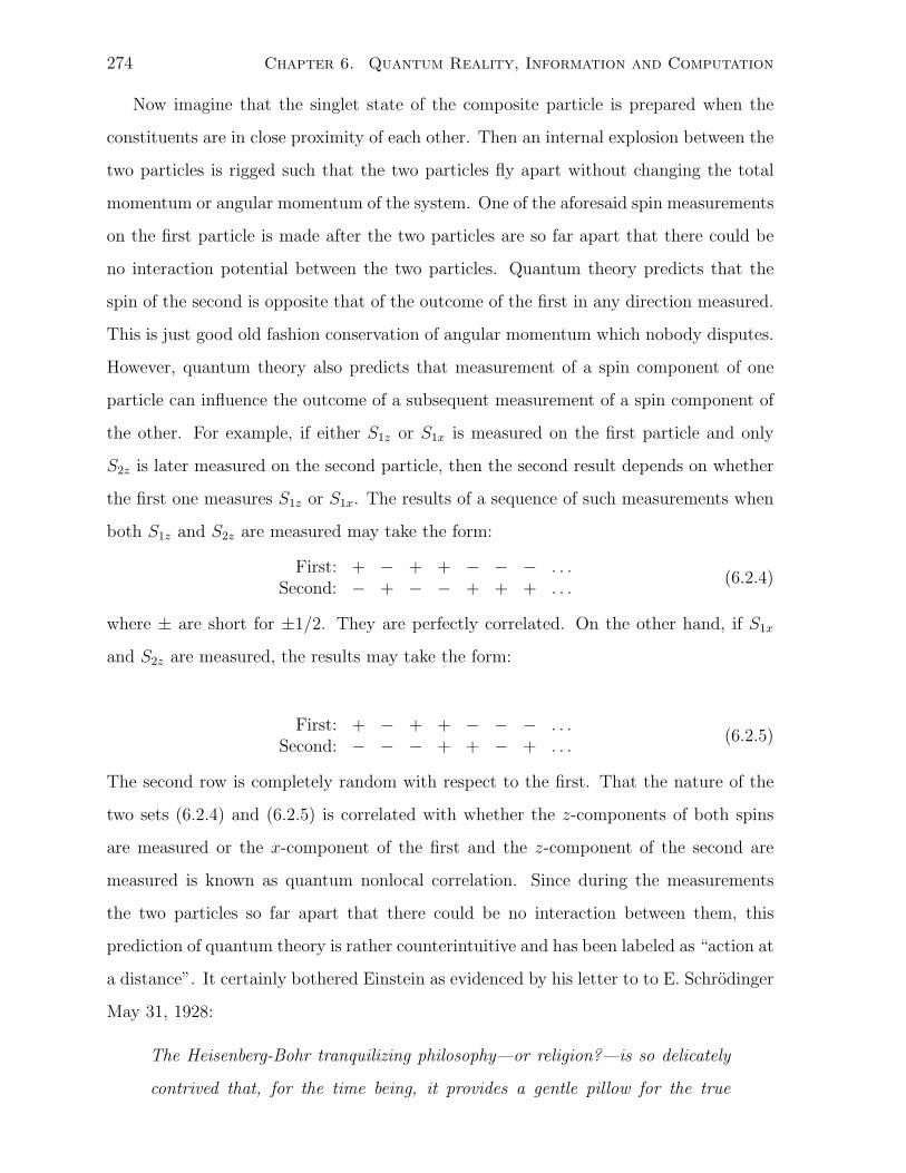
274 Chapter 6. Quantum Reality, Information and Computation
Now imagine that the singlet state of the composite particle is prepared when the
constituents are in close proximity of each other. Then an internal explosion between the
two particles is rigged such that the two particles fly apart without changing the total
momentum or angular momentum of the system. One of the aforesaid spin measurements
on the first particle is made after the two particles are so far apart that there could be
no interaction potential between the two particles. Quantum theory predicts that the
spin of the second is opposite that of the outcome of the first in any direction measured.
This is just good old fashion conservation of angular momentum which nobody disputes.
However, quantum theory also predicts that measurement of a spin component of one
particle can influence the outcome of a subsequent measurement of a spin component of
the other. For example, if either S1z or S1x is measured on the first particle and only
S2z is later measured on the second particle, then the second result depends on whether
the first one measures S1z or S1x. The results of a sequence of such measurements when
both S1z and S2z are measured may take the form:
First: + − + + − − − . . .Second: − + − − + + + . . .
(6.2.4)
where ± are short for ±1/2. They are perfectly correlated. On the other hand, if S1x
and S2z are measured, the results may take the form:
First: + − + + − − − . . .Second: − − − + + − + . . .
(6.2.5)
The second row is completely random with respect to the first. That the nature of the
two sets (6.2.4) and (6.2.5) is correlated with whether the z-components of both spins
are measured or the x-component of the first and the z-component of the second are
measured is known as quantum nonlocal correlation. Since during the measurements
the two particles so far apart that there could be no interaction between them, this
prediction of quantum theory is rather counterintuitive and has been labeled as “action at
a distance”. It certainly bothered Einstein as evidenced by his letter to to E. Schrodinger
May 31, 1928:
The Heisenberg-Bohr tranquilizing philosophy—or religion?—is so delicately
contrived that, for the time being, it provides a gentle pillow for the true
6.2. The EPR Paradox and Bell’s Inequalities 275
believer from which he cannot very easily be aroused. So let him lie there.
6.2.2 EPR Paradox and Einstein’s Locality Hypothesis
The key points of the EPR arguments are:
1. They gave a definition for an element of physical reality:
If, without in any way disturbing a system, we can predict with certainty
(i.e, with probability equal to unity) the value of physical quantity, then
there exists an element of physical reality corresponding to this physical
quantity.
2. For two noncommuting observables, such S2z and S2x, knowing the value of one
precisely means the values of the other is not known. EPR would describe it as when
the z-component of the spin is known, the x-component has no physical reality. It
follows that either that two physical properties represented by two noncommuting
operators “cannot have simultaneous reality” or that “the quantum mechanical
description of reality ... is not complete.”
3. Now take the entangled spin state of two particles. Measurement of S1z yields, say,
the value of +1/2. Then the observable S2z of the second particle would have the
value −1/2 without any measurement. If then S2x is measured, say, with a value
+1/2, then the second particle has a definite value. EPR asserted what has become
known as Einstein’s locality principle. When the two particles are far apart, there
is no interaction. Therefore the experiments on the first particle cannot influence
the properties of the second. Thus, the physical quantities represented by the
noncommuting observables S2z and S2x are shown to “have simultaneous reality”.
This eliminates the first of the two alternatives in statement No. 2, leading to the s
conclusion that the quantum mechanical description of reality given by the original
wave function is not complete.
The latter conclusion led to attempts to find “hidden variables” to supplement the
quantum theory.
276 Chapter 6. Quantum Reality, Information and Computation
Niels Bohr’s rebuttal invoked the concept of complementarity for a complete descrip-
tion of two noncommuting observables.
6.2.3 Bell’s Inequalities
The EPR paradox indicates a choice between the quantum nonlocal correlation and the
Einstein locality hypothesis. A Bell’s inequality is derived from a model observing the
Einstein locality. It can then be compared the quantum prediction. For cases in which
the two results disagree, experiment can then falsify one of the two assertions. Consider
a model which is consistent with the Einstein locality. Let φ and χ be two particles of
spin 1/2, each of which is given two physical attributes mz and m′x of spin directions
along z and x, where m, m′ = ±. Each one of the four possible states of φ is φ(mz, m′x)
and similarly for χ. A composite of φ and χ of total spin zero has four possible states,
φ(mz, m′x)χ(mz, m′x), where m = −m. We make an ensemble of a large number of
replicas of the composite particles, with a quarter of them in each state. The statistical
average of the measurements in either z or x direction for either particle will be consistent
with the quantum theory. The model is consistent with the Einstein locality in the sense
that the outcome of a measurement on one particle is independent of the measurements
which have been done on the other particle.
Now consider making measurements in three different directions along unit vectors
a, b, c (which should not be mutually orthogonal). Let the fraction of the composite
particles in the ensemble in the state φ(a, mb, nc)χ(a, mb, nc) be f(, m, n), where
, m, n = ±. The eight fractions sum to unity. Suppose that Alice measures one of
the three directions on the φ particle and Bob measures a different direction on the χ
particle. The probabilities of the φ particle having the same spin up or down in any two
directions are given by
∑
m=±Pφ(ma, mb) = f(+, +, +) + f(+, +,−) + f(−,−, +) + f(−,−,−); (6.2.6)
∑
m=±Pφ(mb, mc) = f(+, +, +) + f(−, +, +) + f(+,−,−) + f(−,−,−); (6.2.7)
∑
m=±Pφ(mc, ma) = f(+, +, +) + f(+,−, +) + f(−, +,−) + f(−,−,−). (6.2.8)
Thus, the sum of the conditional probabilities that the spin states of φ in any two
6.2. The EPR Paradox and Bell’s Inequalities 277
directions are both up or down is given by
Pφ(same) = 1 + 2f(+, +, +) + 2f(−,−,−) ≥ 1. (6.2.9)
This is one of the Bell inequalities. This is a consequence of the model which satisfies
the Einstein locality.
What does the quantum theory predict for Pφ(same)? The probability Pφ(+a, +b) is
the same as that of Alice obtaining spin-up in the a-direction for φ and Bob obtaining
spin-down in the b-direction for χ,
Pφ(+a, +b) = |〈φ+aχ−b|Ψ0,0〉|2
= |〈φ+aχ−b|√
1
2(|φ+aχ−a〉 − |φ−aχ+a〉) |2
=1
2|〈φ+aχ−b|φ+aχ−a〉|2
=1
2|〈χ−b|χ−a〉|2. (6.2.10)
using the singlet expression, Eq. (6.2.1) in the a-direction. If we align a with the z-axis
and b at an angle θab from the z axis, the transformation matrix yields the matrix element
〈χ−b|χ−a〉 and thus,
Pφ(+a, +b) =1
2cos2
(θab
2
)
. (6.2.11)
In the same manner, we can obtain the same expression for Pφ(−a,−b) and, hence,
Pφ(same) = cos2
(θab
2
)
+ cos2
(θbc
2
)
+ cos2
(θca
2
)
. (6.2.12)
That the quantum prediction is different from the locality result can be seen from the
fact that Eq. (6.2.12) does not always obey the Bell inequality (6.2.9), e.g., when the
three directions are coplanar and the angle between each pair is 2π/3:
Pφ(same) = 3/4. (6.2.13)
The two distinct consequences of Einstein’s locality and of quantum nonlocal correlation
can then be subjected to experimental tests. As mentioned above, experimental results
favor the quantum conclusion (see Problem 2).
278 Chapter 6. Quantum Reality, Information and Computation
6.3 Rudiments of Quantum Information
The discussion on EPR and the Bell inequalities also brings out the concept of the
entangled states which are the underpinning of the processing of quantum information
and which are also useful in quantum computation.
Rolf Landauer illustrated the cornerstone of his study of the energy and entropy
of classical computation processes by the succinct sentence that information is physical.
Each piece of information has to be expressed as a physical state. So you may take comfort
in the fact that the famous information highway cannot be built without physics. As the
physical system storing a bit of information gets smaller and smaller, quantum effects
come into play. As the ultimate quantum system, the two-state system seems to be ideal
for the storage of a bit, know as the qubit (quantum bit). The trick is then to be able
to isolate it from the uncontrolled environment effects. As the amount of information
(number of bits) becomes enormous, the qubits have to be well isolated from one another
and from the environment or else rapid decoherence will set in and the system will obey
the laws of thermodynamics. The remarkable development in the last decade has been
to show how in principle quantum effects may be used to advantage in the science of
information. In this section, we give a flavor of the concepts involved as rather novel and
fun applications of the theory of two-state systems which we have just examined.
6.3.1 Quantum Cryptography
On hearing the EPR experiment, “Aha”, you say,“Alice can now communicate with Bob
at a rate faster than the speed of light.” Suppose Alice goes to Anchorage and Bob to
Barbados. Calvin in California sends at periodic intervals from each singlet composite
of two particles a particle to Alice and a particle to Bob. It has been prearranged that
both of them will measure the spin in the same z direction. It is true that if Alice finds
a spin-up state, Bob will find a spin-down state. However, Alice gets an up or down
state randomly. So all Bob will get is a photo-negative copy of the random sequence,
Eq. (6.2.4), which contains no information.
Let us modify the information transmission protocol somewhat. Alice measures either
Sz or Sx without telling Bob which but she emails Bob her data as a sequence of pluses
6.3. Rudiments of Quantum Information 279
and minuses. Bob then does his measurements of Sz and compare his sequence with
Alice’s. If they are exactly opposite (except for a few errors), then he can deduce that
she measured Sz. If the results correlate only half of the time, then she measured Sx.
This seems a very clumsy way to communicate: not only is it no longer faster than the
speed of light but Alice has to send Bob many bits of information to convey just one
bit. However, if we think of it not as a means for communication but as a means for
cryptography, it is rather robust. Anyone who intercepts the email message has no means
to decode the message of which direction Alice has measured unless the person possesses
the “key”, i.e., the particles which are sent to Bob. How to discover if the particles have
been intercepted and then resent to Bob will be left as an exercise for the reader.
The above is an example of a quantum public key distribution in the public key
cryptography. For an accessible discussion, see [18].
6.3.2 A Qubit
The fundamental unit of information is a bit which is a state such as 0 or 1 in a classical
two-state system. The state of a quantum bit, now called a qubit, is a state in the Hilbert
space of all possible states in a quantum two-state system. For the sake of familiarity,
we shall use the two basis states to be |±〉, or the spin-up and down states along a
specified direction. For definiteness, we shall take the basis set |+〉, |−〉 to represent 1, 0
respectively. A qubit represents more than just the possibility of one of these two states
to include any superposition of them. The restriction of normalization and the removal
of an overall phase yield two real numbers (p, θ) to characterize a qubit:
|ψ〉 = | + 1〉peiθ + | − 1〉√
1 − p2. (6.3.1)
To “read” the qubit (to retrieve the information) requires measurements on this state,
the outcome of which we have examined.
6.3.3 Entangled States and Quantum Operations
As in the classical information processing, the quantum counterpart also requires logical
operations involving two qubits. The composite system of two spin-1/2 particles has
four states. As eigenstates of the total angular momentum J2 and Jz, two of the triplet
280 Chapter 6. Quantum Reality, Information and Computation
states, |+, +〉 and |−,−〉, are unentangled product states. Measurement of spin on one
does not disturb the state of the other. One may also say that the spin states of the two
particles are uncorrelated. By contrast, the triplet state Ψ1,0 and the singlet state Ψ0,0
are sums of product states, i.e., entangled states. We have seen that, in an entangled
state, measurement on one spin can affect the outcome of the subsequent measurement
of the other spin. This property provides the important distinction between classical and
quantum information.
Consider coding two classical bits of information in two qubits. The straightforward
way is to store the information in four unentangled states:
|±,±〉 ≡ |±〉|±〉. (6.3.2)
It is sometimes advantageous to encode the information in four entangled states, known
as the Bell states or EPR pairs,
|Ψ±〉 =1√2(|+,−〉 ± |−, +〉)
|Φ±〉 =1√2(|+, +〉 ± |−,−〉). (6.3.3)
We have seen one example in quantum cryptography and we shall see more presently.
To find a transformation from the unentangled states to the Bell states, we consider
first a useful single-spin transformation known as the Hadamard transform
H =1√2(σx + σz) =
1√2
[1 11 −1
]
. (6.3.4)
It transform the basis states |m〉, m = ±1 into two superposition states (|+〉+m|−〉)/√
2.
It is convenient to introduce a quantum circuit diagram to depict the operation (Fig. 6.1(a)).
A most important transformation involving two qubits is the logic operation, XOR
or controlled-NOT (C-NOT) (Fig. 6.1(b)),
CN |m, n〉 = |m, mn〉. (6.3.5)
The first bit may be regarded as the source or control, whose spin direction determines
how the second bit (known as the target) is changed. Thus, if the source is −, the
target state is unchanged and if the source is +, the target is flipped (|n〉 → |n〉).
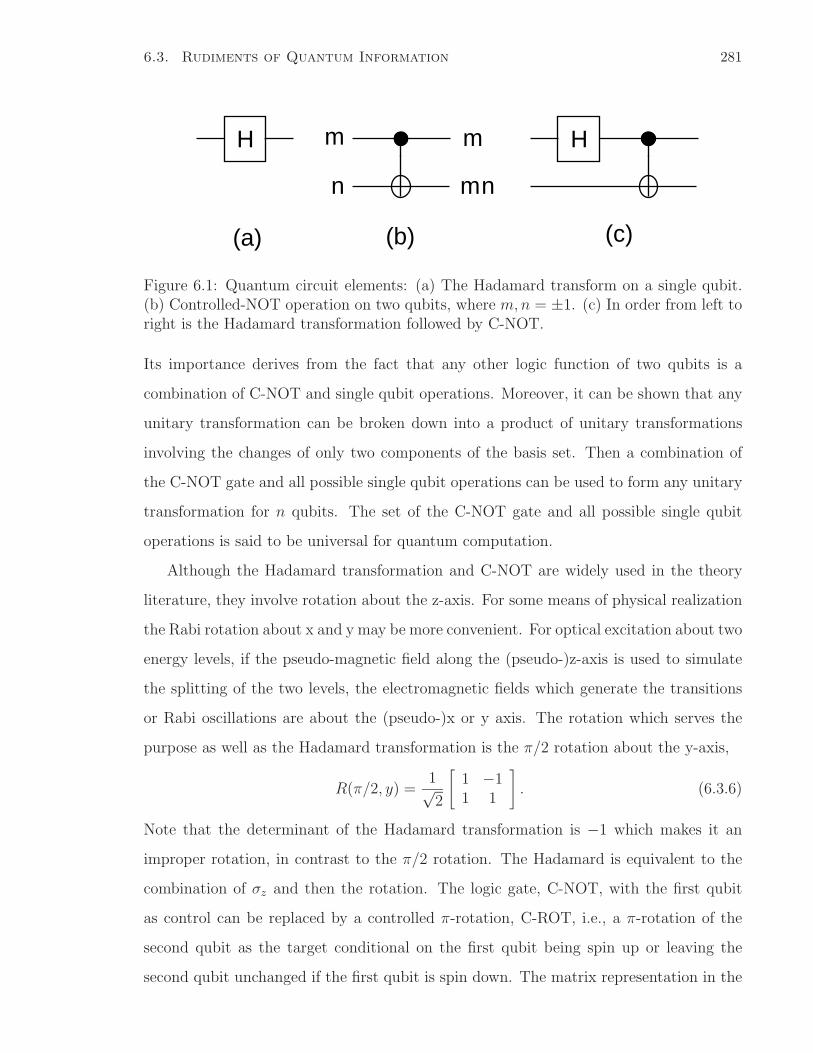
H m
n mn
m H
(a) (b) (c)
6.3. Rudiments of Quantum Information 281
Figure 6.1: Quantum circuit elements: (a) The Hadamard transform on a single qubit.(b) Controlled-NOT operation on two qubits, where m, n = ±1. (c) In order from left toright is the Hadamard transformation followed by C-NOT.
Its importance derives from the fact that any other logic function of two qubits is a
combination of C-NOT and single qubit operations. Moreover, it can be shown that any
unitary transformation can be broken down into a product of unitary transformations
involving the changes of only two components of the basis set. Then a combination of
the C-NOT gate and all possible single qubit operations can be used to form any unitary
transformation for n qubits. The set of the C-NOT gate and all possible single qubit
operations is said to be universal for quantum computation.
Although the Hadamard transformation and C-NOT are widely used in the theory
literature, they involve rotation about the z-axis. For some means of physical realization
the Rabi rotation about x and y may be more convenient. For optical excitation about two
energy levels, if the pseudo-magnetic field along the (pseudo-)z-axis is used to simulate
the splitting of the two levels, the electromagnetic fields which generate the transitions
or Rabi oscillations are about the (pseudo-)x or y axis. The rotation which serves the
purpose as well as the Hadamard transformation is the π/2 rotation about the y-axis,
R(π/2, y) =1√2
[1 −11 1
]
. (6.3.6)
Note that the determinant of the Hadamard transformation is −1 which makes it an
improper rotation, in contrast to the π/2 rotation. The Hadamard is equivalent to the
combination of σz and then the rotation. The logic gate, C-NOT, with the first qubit
as control can be replaced by a controlled π-rotation, C-ROT, i.e., a π-rotation of the
second qubit as the target conditional on the first qubit being spin up or leaving the
second qubit unchanged if the first qubit is spin down. The matrix representation in the
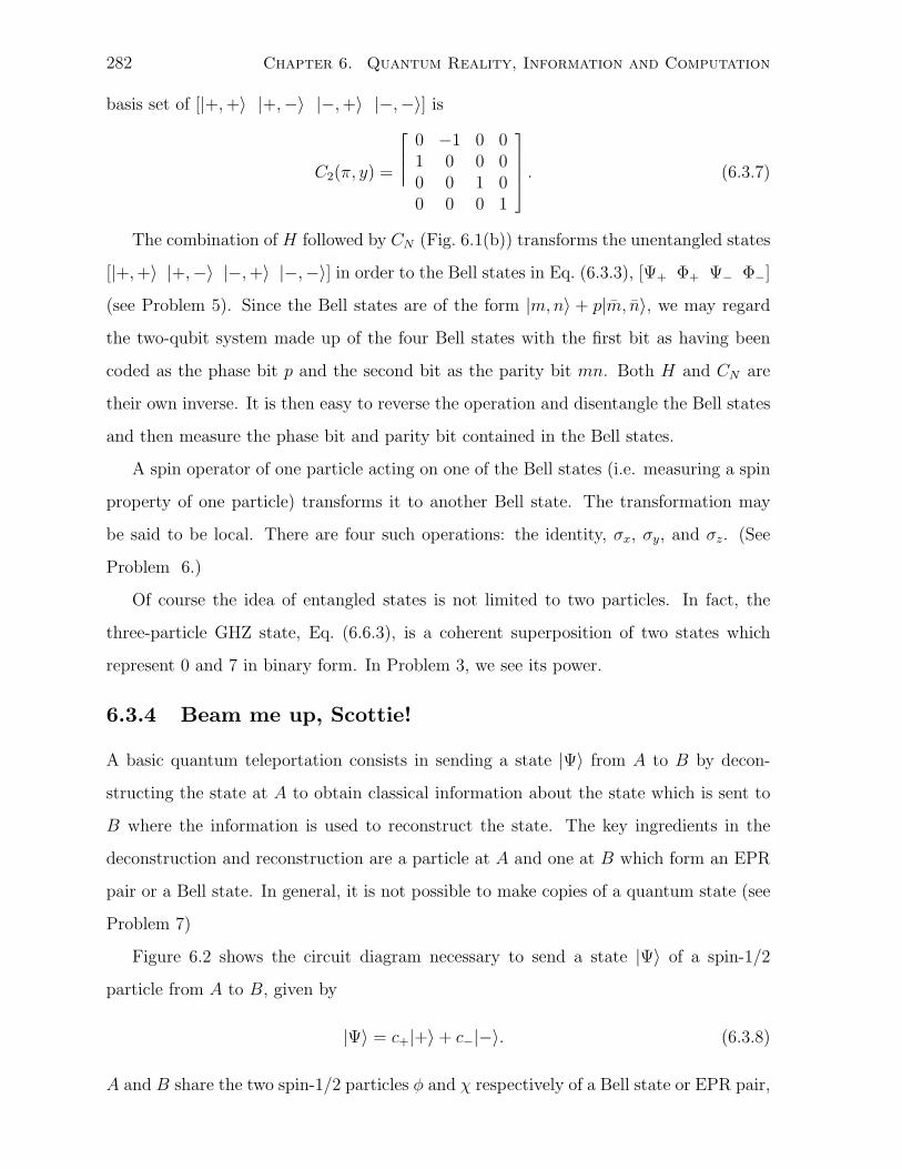
282 Chapter 6. Quantum Reality, Information and Computation
basis set of [|+, +〉 |+,−〉 |−, +〉 |−,−〉] is
C2(π, y) =
0 −1 0 01 0 0 00 0 1 00 0 0 1
. (6.3.7)
The combination of H followed by CN (Fig. 6.1(b)) transforms the unentangled states
[|+, +〉 |+,−〉 |−, +〉 |−,−〉] in order to the Bell states in Eq. (6.3.3), [Ψ+ Φ+ Ψ− Φ−]
(see Problem 5). Since the Bell states are of the form |m, n〉 + p|m, n〉, we may regard
the two-qubit system made up of the four Bell states with the first bit as having been
coded as the phase bit p and the second bit as the parity bit mn. Both H and CN are
their own inverse. It is then easy to reverse the operation and disentangle the Bell states
and then measure the phase bit and parity bit contained in the Bell states.
A spin operator of one particle acting on one of the Bell states (i.e. measuring a spin
property of one particle) transforms it to another Bell state. The transformation may
be said to be local. There are four such operations: the identity, σx, σy, and σz. (See
Problem 6.)
Of course the idea of entangled states is not limited to two particles. In fact, the
three-particle GHZ state, Eq. (6.6.3), is a coherent superposition of two states which
represent 0 and 7 in binary form. In Problem 3, we see its power.
6.3.4 Beam me up, Scottie!
A basic quantum teleportation consists in sending a state |Ψ〉 from A to B by decon-
structing the state at A to obtain classical information about the state which is sent to
B where the information is used to reconstruct the state. The key ingredients in the
deconstruction and reconstruction are a particle at A and one at B which form an EPR
pair or a Bell state. In general, it is not possible to make copies of a quantum state (see
Problem 7)
Figure 6.2 shows the circuit diagram necessary to send a state |Ψ〉 of a spin-1/2
particle from A to B, given by
|Ψ〉 = c+|+〉 + c−|−〉. (6.3.8)
A and B share the two spin-1/2 particles φ and χ respectively of a Bell state or EPR pair,
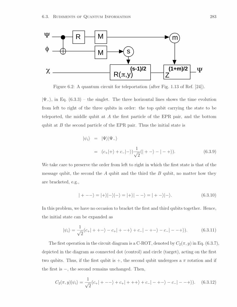
Ψ
χ
R M m
sM
(1+m)/2(s-1)/2R(π,y)
φ
ZΨ
6.3. Rudiments of Quantum Information 283
Figure 6.2: A quantum circuit for teleportation (after Fig. 1.13 of Ref. [24]).
|Ψ−〉, in Eq. (6.3.3) – the singlet. The three horizontal lines shows the time evolution
from left to right of the three qubits in order: the top qubit carrying the state to be
teleported, the middle qubit at A the first particle of the EPR pair, and the bottom
qubit at B the second particle of the EPR pair. Thus the initial state is
|ψi〉 = |Ψ〉|Ψ−〉
= (c+|+〉 + c−|−〉) 1√2(| + −〉 − | − +〉). (6.3.9)
We take care to preserve the order from left to right in which the first state is that of the
message qubit, the second the A qubit and the third the B qubit, no matter how they
are bracketed, e.g.,
| + −−〉 = |+〉|−〉|−〉 = |+〉| − −〉 = | + −〉|−〉. (6.3.10)
In this problem, we have no occasion to bracket the first and third qubits together. Hence,
the initial state can be expanded as
|ψi〉 =1√2(c+| + +−〉 − c+| + −+〉 + c−| − +−〉 − c−| − −+〉). (6.3.11)
The first operation in the circuit diagram is a C-ROT, denoted by C2(π, y) in Eq. (6.3.7),
depicted in the diagram as connected dot (control) and circle (target), acting on the first
two qubits. Thus, if the first qubit is +, the second qubit undergoes a π rotation and if
the first is −, the second remains unchanged. Then,
C2(π, y)|ψi〉 =1√2(c+| + −−〉 + c+| + ++〉 + c−| − +−〉 − c−| − −+〉). (6.3.12)
284 Chapter 6. Quantum Reality, Information and Computation
Note that the middle qubit in the first and second terms on the right are changed.
The second operation is the π/2 rotation about the y-axis denoted by R acting on
the first qubit:
R|+〉 =1√2(|+〉 + |−〉),
R|−〉 =1√2(−|+〉 + |−〉). (6.3.13)
The result of the second operation is
RCN |ψi〉 =1
2[c+(| + −−〉 + | − −−〉 + | + ++〉 + | − ++〉)
+c−(−| + +−〉 + | − +−〉 + | + −+〉 − | − −+〉)]
=1
2[| + +〉(c+|+〉 − c−|−〉) + | + −〉(c−|+〉 + c+|−〉)
+| − +〉(c+|+〉 + c−|−〉) + | − −〉(−c−|+〉 + c+|−〉)]. (6.3.14)
In the last step, we have expressed the state in terms of the spin states of the first two
qubits. If their spin states (Sz) are measured, as indicated by the boxes M , the state will
end up in one of the states |ms〉, where m and s are the spin directions of the message
bit and the sender’s bit. The receiver qubit will end up in the corresponding state in the
last step of Eq. (6.3.14). For example, if the measured result is (m, s) = (−, +), then the
qubit at the receiver’s end B becomes the state |Ψ〉. In general, if the measured state
is |ms〉, the single-qubit operations Z(m+1)/2R(π, y)(s−1)/2 will bring the third qubit at B
to the state |Ψ〉, where Z is the operator σz.
Since the state at B cannot be measured without destroying it, the classical informa-
tion (m, s) from the sender is indispensable in reconstructing the teleported state. This
message sending keeps the whole teleportation speed below that of light. Note that a way
to view the teleportation is that a shared EPR pair and two classical bits of information
are equivalent to one qubit of communication.
6.3.5 You’ve Got Mail
Although we have craftily turned the failure of the first attempt at quantum communi-
cation into quantum cryptography, the question of how Alice and Bob can communicate
6.4. A Brief Introduction to Quantum Computation 285
with entangled states remains. Here is an example of applying entanglement to commu-
nication. As before, Calvin prepares two spins in a standard Bell state and send φ to
Alice and χ to Bob. Alice can perform on φ one of the four local operations and thereby
changes the Bell state Calvin of CalComm prepared into one of the four possible Bell
states. Now, she sends her particle to Bob who is, thus, in possession of the two particles
in the new Bell state. A C-NOT followed by a Hadamard operation will give Bob one of
the unentangled states which he can determine by spin measurements on both particles.
Thus, he knows the new Bell state and, hence, the two (classical) bits of information
Alice sends him (cf. Sec. 6.3.3). The company CalComm which sells the communication
equipment and protocol advertises that Alice can send two bits of information to Bob
with one photon (utilizing its polarization states – see Problem 10 in Chapter 5). This is
an example of “dense coding”. Consumer Advocate points out that, of course, Bob also
needs the photon CalComm sends him. Nonetheless, Alice’s information may be sent to
Bob regardless of the information content of the photons sent out by CalComm. The
added bonus is that the information is interception-proof.
6.4 A Brief Introduction to Quantum Computation
A knowledge of quantum computing is timely, but more important to the learning of
quantum theory is the fact that quantum computing provides a wonderful framework to
understand how quantum theory works in the microscopic components of the computer
and the consequence of their interaction with the macroscopic world, in the preparation
of the initial state, in the dissipative and dephasing effects of the environment, and in
the measurement of the finite state of the quantum computation.
Richard Feynman noted the rapid increase of steps required to simulate the time
evolution of a quantum system as the number of particles in the system rises. He sug-
gested using an analog quantum computer to simulate the dynamics of a whole class of
quantum systems. P. Benioff introduced the notion of building a universal computer (a
Turing machine) based on the quantum system. In this section, we introduce the key
ideas of quantum computation. First, we illustrate the power of quantum computation
through “parallel processing” by studying the Deutsch-Josza algorithm. Then we discuss
286 Chapter 6. Quantum Reality, Information and Computation
the basic components for a universal computer. An examination of the dephasing effects
of the environment on the quantum computer leads to the concept of decoherence, which
we will examine more generally in the following section.
6.4.1 The Deutsch-Josza algorithm
David Deutsch [11] pointed out that the potential of quantum computing lies in “quantum
parallelism”. He posed the following problem of conditional branching. Suppose we have
already a program which computes f(x) if x is given. In the simple example of two bits,
(x = ±1, f(x) = ±1), there are four possible functions to produce f(+1) and f(−1).
Deutsch’s problem is how to use quantum theory to arrange the evaluation of f(x) to
determine if the function is constant (f(+1) = f(−1)) or balanced (the function yields
the ±1 values equally). The classical way takes two evaluations and then comparison of
the two results. Now consider a quantum program for f(x) using a transformation which
is a relative of C-NOT:
Uf |m, n〉 = |m, f(m)n〉. (6.4.1)
A state is first prepared in the ground state |−,−〉. A Hadamard transform is used on
the second bit, to yield
| − x〉 =1√2(|+〉 − |−〉). (6.4.2)
Then the Hadamard transform is used on the first bit of the state |+,−〉):
| + x〉 =1√2(|+〉 + |−〉). (6.4.3)
The result is a mapping from |−,−〉 to |+ x,−x〉. Then the operation Uf is used on the
rotated product state, resulting in
Uf | + x,−x〉 =1√2
[(−1)[f(+1)−1]/2| + 1,−x〉 + (−1)[f(−1)−1]/2| − 1,−x〉
]. (6.4.4)
If the function f is constant, the resultant state is |+x,−x〉 and, if not, it is the resultant
state is |−x,−x〉. Which of these states can be determined by measuring the x component
of the spin of the first bit.
The contrast between the classical program and the quantum one is in the use of the
subroutine for evaluation of the function f(x). The classical program submits each value
6.4. A Brief Introduction to Quantum Computation 287
of x for a separate evaluation of the function. The power of the quantum computation
comes from the use of the linear superposition of two states in both the input and output
qubits for one linear transformation. It means that the information can be spread into
both states of the same bit and that parallel processing is possible. The implementation
of the Deutsch-Jozsa algorithm by nuclear magnetic resonance has been carried out.
6.4.2 Requirements for quantum computation
We describe a simple conceptual quantum computer and its operations. There are inge-
nious alternatives but we are contented with illustrating the essential ideas. The physical
components of a quantum computer are a set of subsystems in which the qubit can be
coded. The simplest example is a system of spin 1/2 particles. There should be negligible
interaction between any two qubits except under control of the program when it is desired
to run a logic gate operation between two qubits. There should be as little interaction
as possible with the environment since irreversible processes are deleterious to the ideal
quantum computing process consisting of a series of linear, reversible transformations.
The only exceptions are the initialization of the state of the quantum computer and the
measurement at the end of the computing process where the macroscopic instrument
must intervene. The initialization may be as simple as cooling the computer to the
ground state. Note that this is an irreversible process and would take a very long time
if the temperature is not sufficiently low compared with the energy spacing between the
two qubit states.
A computation on a quantum computer consists in applying a single unitary operation
on the n qubits of this system. In order that the computer is flexible and not just for
a single purpose, one scenario is to render the operations on the qubits as composed of
controlled single qubit dynamics and two-qubit conditional dynamics described above.
A computing process could consist of a controlled sequence of such operations. It is
sufficient to have at hand a set of arbitrary one qubit rotations and the CNOT logic
gate in order to make up a sequence of operations which result in any desired unitary
operation of the n qubits. This is known as universal computation. This greatly simplifies
the design of physical operations to implement quantum computation.
A classical computation procedure involves processing information stored in bits us-
288 Chapter 6. Quantum Reality, Information and Computation
ing a sequence of elementary logic operations on two bits. The corresponding elementary
quantum gate performs an elementary operation on two qubits, which is just a unitary
transformation. The C-NOT is an example. Such an operation has been demonstrated
recently in experiments using trapped atoms, cavity quantum electrodynamics, and nu-
clear magnetic resonance. More generally, a quantum computation for n qubits involves
a sequence of unitary transformations. Thus, every operation has an inverse and is re-
versible. In classical computation, there are also reversible gates. However, unlike the
quantum case, not all gates have to be reversible. A logic gate like NAND combines the
input of two bits into a one-bit result. The procedure cannot be reversed.
The algorithm to solve the Deutsch problem and to illustrate the aspect of parallel
processing in quantum computation can be generalized to any number of qubits. A
physical system which can implement a generalization to a large number of qubits is said
to be scalable. In the quantum procedure, the initial information has to be coded and
the final outcome measured. So at these stages, it has no advantage over the classical
procedure. However, the intermediate transformations handle the bits in parallel and
possess a much higher efficiency. In theory, the power of quantum computing was first
demonstrated dramatically by Peter Shor in factorizing a large integer. It is commonly
believed (but not proven) that to factorize an integer of N digits by a classical algorithm
requires the number of steps exponential in N . Shor showed that a quantum algorithm
requires the number of steps which is a polynomial in N . Since the best current encryption
schemes depend on the near impossibility of factorization, this has vast implication on
cryptography, much used in electronic banking and other online commerce. The key
in the quantum factorization scheme is the quantum Fourier transform, which has a
number of other applications. Another famous quantum algorithm was constructed by
L.K. Grover for searching an unsorted list. A classical search mechanism takes O(N)
steps for a long list of N items. Grover’s algorithm takes O(√
N) steps.
The requirement of weak interaction between the qubits and the environment stems
from the fact that the dephasing dynamics causes the final state to deviate from the
ideal design. This requirement brings into sharp relief the decoherence effect. Since the
phenomenon is of importance to the general quantum theory in the interplay between the
6.5. Decoherence 289
dynamics of the microscopic and macroscopic systems, we shall devote the next section
to it.
One major development not touched upon is the quantum error correction. The error
in the intermediate states which occurs because either of the environment dephasing or
of unintended dynamics due to the intrusion of the states in the system not designed for
the qubits can be corrected by making replicates of each qubit and by designing quantum
operations which automatically change the state of the set of all replicas of a qubit to
the one assumed by the majority. The error correction is not sure fire but can have a
very high success rate.
We have only given a flavor of the excitement of the recent development in this group
of applications of quantum mechanics. There are major efforts devoted to the quantum
algorithms as well as to the implementation of these ideas in real physical systems.
6.5 Decoherence
6.5.1 Dephasing and decoherence
It is shown in Section 5.6 that a two-state system in contact with a reservoir develops
irreversible dynamical processes which can be separated into dissipation and dephasing.
Dissipation is present in the transition from one state to another, represented by the
damping terms in the diagonal part of the density matrix, known as the population terms.
Dephasing refers to the loss of phase coherence between the two states, represented by the
decay of the off-diagonal term of the density matrix, also known as the coherence term.
The dephasing varies over a wide range of values for different systems, depending on the
strength of interaction with the environment. For the nuclear spins in a liquid or solid,
it could be seconds or much longer; for the electron spins, of the order of milliseconds;
for two levels in an atom which suffers radiative recombination, 10 ns; and, for two levels
in a semiconductor quantum dot, 100 ps.
The question before us now is what is the dephasing time between two states of
a macroscopic system, i.e., one with the number of degrees of freedom closer to the
Avogadro’s number A than to unity. The question is posed most starkly as the problem
of Schrodinger’s cat. The system consists of a single atom with two states, a Geiger
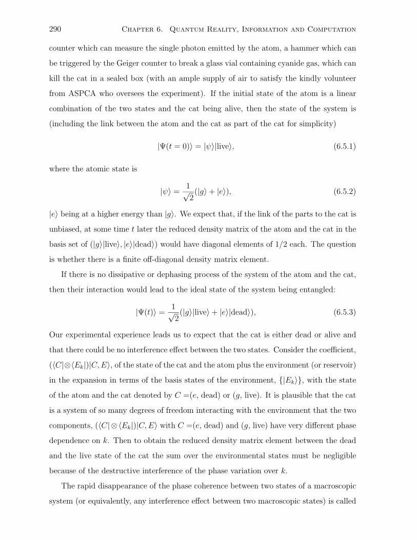
290 Chapter 6. Quantum Reality, Information and Computation
counter which can measure the single photon emitted by the atom, a hammer which can
be triggered by the Geiger counter to break a glass vial containing cyanide gas, which can
kill the cat in a sealed box (with an ample supply of air to satisfy the kindly volunteer
from ASPCA who oversees the experiment). If the initial state of the atom is a linear
combination of the two states and the cat being alive, then the state of the system is
(including the link between the atom and the cat as part of the cat for simplicity)
|Ψ(t = 0)〉 = |ψ〉|live〉, (6.5.1)
where the atomic state is
|ψ〉 =1√2(|g〉 + |e〉), (6.5.2)
|e〉 being at a higher energy than |g〉. We expect that, if the link of the parts to the cat is
unbiased, at some time t later the reduced density matrix of the atom and the cat in the
basis set of (|g〉|live〉, |e〉|dead〉) would have diagonal elements of 1/2 each. The question
is whether there is a finite off-diagonal density matrix element.
If there is no dissipative or dephasing process of the system of the atom and the cat,
then their interaction would lead to the ideal state of the system being entangled:
|Ψ(t)〉 =1√2(|g〉|live〉 + |e〉|dead〉), (6.5.3)
Our experimental experience leads us to expect that the cat is either dead or alive and
that there could be no interference effect between the two states. Consider the coefficient,
(〈C|⊗〈Ek|)|C, E〉, of the state of the cat and the atom plus the environment (or reservoir)
in the expansion in terms of the basis states of the environment, |Ek〉, with the state
of the atom and the cat denoted by C =(e, dead) or (g, live). It is plausible that the cat
is a system of so many degrees of freedom interacting with the environment that the two
components, (〈C|⊗〈Ek|)|C, E〉 with C =(e, dead) and (g, live) have very different phase
dependence on k. Then to obtain the reduced density matrix element between the dead
and the live state of the cat the sum over the environmental states must be negligible
because of the destructive interference of the phase variation over k.
The rapid disappearance of the phase coherence between two states of a macroscopic
system (or equivalently, any interference effect between two macroscopic states) is called
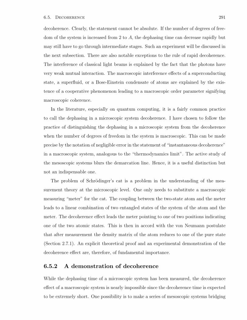
6.5. Decoherence 291
decoherence. Clearly, the statement cannot be absolute. If the number of degrees of free-
dom of the system is increased from 2 to A, the dephasing time can decrease rapidly but
may still have to go through intermediate stages. Such an experiment will be discussed in
the next subsection. There are also notable exceptions to the rule of rapid decoherence.
The interference of classical light beams is explained by the fact that the photons have
very weak mutual interaction. The macroscopic interference effects of a superconducting
state, a superfluid, or a Bose-Einstein condensate of atoms are explained by the exis-
tence of a cooperative phenomenon leading to a macroscopic order parameter signifying
macroscopic coherence.
In the literature, especially on quantum computing, it is a fairly common practice
to call the dephasing in a microscopic system decoherence. I have chosen to follow the
practice of distinguishing the dephasing in a microscopic system from the decoherence
when the number of degrees of freedom in the system is macroscopic. This can be made
precise by the notation of negligible error in the statement of “instantaneous decoherence”
in a macroscopic system, analogous to the “thermodynamics limit”. The active study of
the mesoscopic systems blurs the demarcation line. Hence, it is a useful distinction but
not an indispensable one.
The problem of Schrodinger’s cat is a problem in the understanding of the mea-
surement theory at the microscopic level. One only needs to substitute a macroscopic
measuring “meter” for the cat. The coupling between the two-state atom and the meter
leads to a linear combination of two entangled states of the system of the atom and the
meter. The decoherence effect leads the meter pointing to one of two positions indicating
one of the two atomic states. This is then in accord with the von Neumann postulate
that after measurement the density matrix of the atom reduces to one of the pure state
(Section 2.7.1). An explicit theoretical proof and an experimental demonstration of the
decoherence effect are, therefore, of fundamental importance.
6.5.2 A demonstration of decoherence
While the dephasing time of a microscopic system has been measured, the decoherence
effect of a macroscopic system is nearly impossible since the decoherence time is expected
to be extremely short. One possibility is to make a series of mesoscopic systems bridging
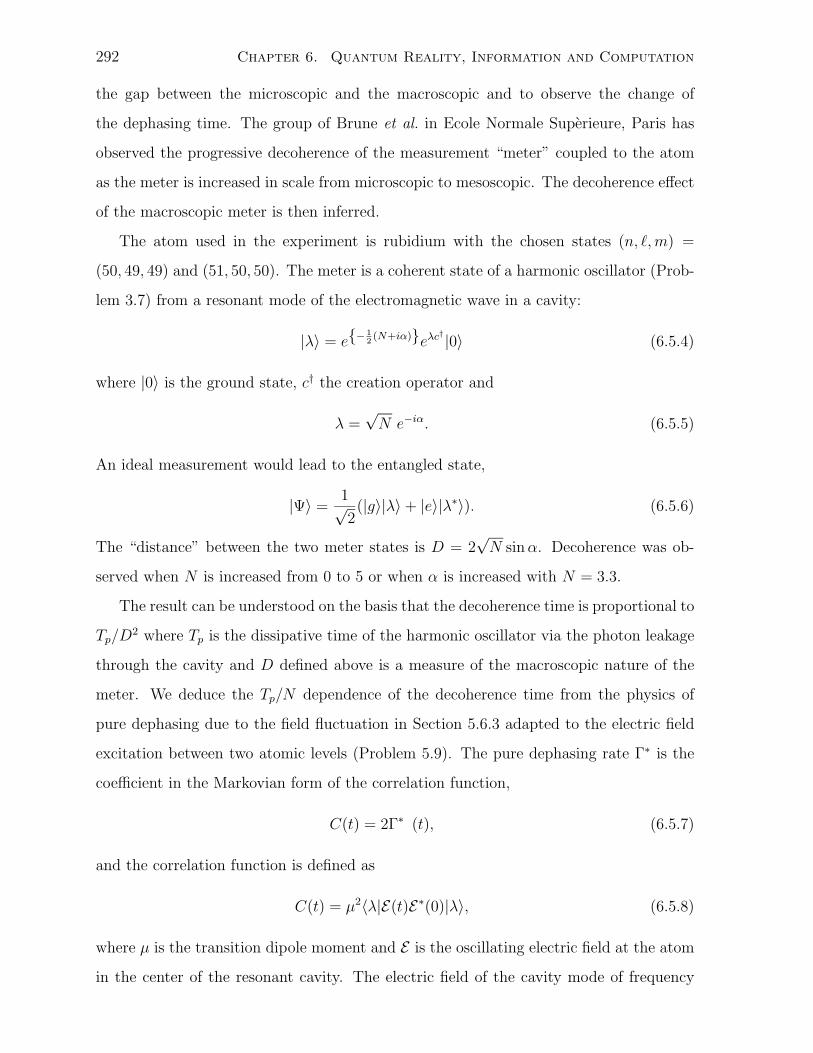
292 Chapter 6. Quantum Reality, Information and Computation
the gap between the microscopic and the macroscopic and to observe the change of
the dephasing time. The group of Brune et al. in Ecole Normale Superieure, Paris has
observed the progressive decoherence of the measurement “meter” coupled to the atom
as the meter is increased in scale from microscopic to mesoscopic. The decoherence effect
of the macroscopic meter is then inferred.
The atom used in the experiment is rubidium with the chosen states (n, , m) =
(50, 49, 49) and (51, 50, 50). The meter is a coherent state of a harmonic oscillator (Prob-
lem 3.7) from a resonant mode of the electromagnetic wave in a cavity:
|λ〉 = e− 12(N+iα)eλc†|0〉 (6.5.4)
where |0〉 is the ground state, c† the creation operator and
λ =√
N e−iα. (6.5.5)
An ideal measurement would lead to the entangled state,
|Ψ〉 =1√2(|g〉|λ〉 + |e〉|λ∗〉). (6.5.6)
The “distance” between the two meter states is D = 2√
N sin α. Decoherence was ob-
served when N is increased from 0 to 5 or when α is increased with N = 3.3.
The result can be understood on the basis that the decoherence time is proportional to
Tp/D2 where Tp is the dissipative time of the harmonic oscillator via the photon leakage
through the cavity and D defined above is a measure of the macroscopic nature of the
meter. We deduce the Tp/N dependence of the decoherence time from the physics of
pure dephasing due to the field fluctuation in Section 5.6.3 adapted to the electric field
excitation between two atomic levels (Problem 5.9). The pure dephasing rate Γ∗ is the
coefficient in the Markovian form of the correlation function,
C(t) = 2Γ∗δ(t), (6.5.7)
and the correlation function is defined as
C(t) = µ2〈λ|E(t)E∗(0)|λ〉, (6.5.8)
where µ is the transition dipole moment and E is the oscillating electric field at the atom
in the center of the resonant cavity. The electric field of the cavity mode of frequency
6.5. Decoherence 293
ωc is in the quantized form related to the harmonic oscillator (in the rotating wave
approximation),
E = E0c, (6.5.9)
where c is the annihilation operator and
E0 =
√hωc
2ε0V, (6.5.10)
V being the cavity volume. The form of E0 comes the consideration of the energy of the
electromagnetic field or from the quantization of the electric field in Chapter 14. If the
damping of the harmonic oscillator is taken as
c(t) = ce−iωct−Γct, (6.5.11)
the solution of Problem 11 yields,
Γ∗ ∝ µ2ε2N
h2Γc
∼ Na3
V
ωc
Γc
R
h, (6.5.12)
using µ ∼ ea, a being the atomic radius. This expression shows the physical origin of the
decoherence rate. It is proportional to N which is a measure of the size of the meter. The
ratio of the atomic volume to the cavity volume is a measure of the coupling strength of
the atom to the meter. The ratio ωc/Γc is the quality factor of the cavity. It is inversely
proportional to the leakage of the cavity mode. R ∼ e2/ε0a is the Ryberg energy of the
atomic state.
294 Chapter 6. Quantum Reality, Information and Computation
6.6 Problems
1. Another Bell Inequality [29]
In the notation of Sec. 6.2.3 for the singlet state, show that from the Einstein
locality
Pφ(+a,−b) ≤ Pφ(+a,−c) + Pφ(+c,−b). (6.6.1)
Find a case where this is contradicted by the quantum prediction.
2. An experimental test of Bell’s inequalities In an experiment by Aspect et al.,
an entangled pair of photons of opposite linear polarizations are measured by two
separate polarizers.
(a) Prove the Bell inequality used. [2].
(b) Write a short account of the experiment or give a 15-minute talk on the ex-
periment.
3. Bell’s Theorem without Inequalities [19]
Consider a composite made of three spin-1/2 particles, labeled a, b, c. In a spin-
conserving separation, they fly off in the same plane in three directions za, zb, zc.
The normal to the common plane is given by the unit vector x. The spin components
along the Cartesian directions x, yj, zj for particle j are given by the Pauli matrices,
σjx, σ
jy, σ
jz, (times h/2 which will be understood), where j = a, b, c. Imagine that
each Stern-Gerlach apparatus is set up along one particle path to measure either
σjx or σj
y when the three particles are far enough apart to have no interaction with
one another. We shall consider in order the predictions (1) of the quantum theory
and (2) of a theory using the Einstein locality for the measurements of the four
observables:
Ka = σaxσ
byσ
cy,
Kb = σayσ
bxσ
cy,
Kc = σayσ
byσ
cx,
6.6. Problems 295
B = σaxσ
bxσ
cx. (6.6.2)
(a) Show that Kj, j = a, b, c form a complete set of three commuting Hermitian
operators and that K2j = 1. Hence, find the eigenvalues of Kj. For the state
|Ψ〉 =1√2
(| + za, +zb, +zc〉 − | − za,−zb,−zc〉) , (6.6.3)
where ±zj denote the spin-up and down states along the zj direction for par-
ticle j, show that it is an eigenstate of each Kj with the eigenvalue +1.
(b) Show that B = −KaKbKc and, hence, that it commutes with each Kj and that
the state Ψ given by Eq. (6.6.3) is also an eigenstate of B but with eigenvalue
−1. Note the minus sign.
(c) Deduce what the quantum theory prediction is for Kj in state Ψ with a si-
multaneous measurement of the x-component of spin for particle j and the
y-components for the other two particles. Deduce also what the prediction
is for B with a simultaneous measurement of the x-components of all three
particles in the state Ψ.
(d) Now construct a theory including the Einstein reality and spin conserva-
tion. This means that when the particles are apart, the spin values of mjx =
±1, mjy = ±1 of each particle in the two directions must be measurable. Make
sure that this theory yields the same predictions for the simultaneous mea-
surement of the x-component of spin for particle j and the y-components for
the other two particles as the quantum theory for Kj in state Ψ. Deduce what
the prediction is for the product maxm
bxm
cx for the simultaneous measurement
of the x-components of all three particles separately according to the locality
theory.
(e) Discuss the contradictions with quantum theory of the two locality results (1)
the values mjx and mj
y are known for particle j and (2) the value of maxm
bxm
cx
for state Ψ.
4. Security of transmission
For the example of quantum cryptography described in Sec. 6.3.1, devise a method
to provide spot checks whether the messages have been intercepted.
296 Chapter 6. Quantum Reality, Information and Computation
5. How to entangle uncorrelated states
(a) Show that a Hadamard transform on the first qubit followed by the controlled-
NOT operation with the first qubit as source and the second qubit as target
can change the two-qubit product states into the four Bell states.
(b) A friend told you that she took one product state, followed the above procedure
and got the Φ− Bell state. What product state did she start with?
(c) If she had used a π/2 rotation about the y-axis followed by a controlled π
rotation as defined in the text, which of the four product states would be
her starting state to reach the Φ− Bell state? Did you or she leave out any
information in this answer? Is it important?
6. Local operations on the Bell states
The phase-shift operation on the Bell states is σφz acting only on the first particle,
φ. The flipping operator is σχx acting only on the second particle χ. Find (in either
order) the transformation matrices and the resultant states of the four operations:
identity, phase-shift, bit-flip, and the combination of phase-shift and bit-flip.
7. Quantum no-cloning theorem
(a) Show that if one starts out with the quantum equivalent of a sheet of black
and white dots and a blank (white) sheet, there is a quantum transformation
to copy the first sheet onto the second.
(b) Consider a close-system with the state space made up of three subspaces
named the “original” and the “copy” with equal number of qubits and the
“machine”. Show that there is no single process that can made copies of all
possible originals.
(c) Show that if the initial state of the original is known (in binary form), then it
is possible to design a special process to make a copy.
8. Teleportation
6.6. Problems 297
(a) Design the circuit for teleportation of a spin-1/2 state starting with, instead
of the singlet state as in the text, the Bell state
|Φ+〉 =1√2(|+, +〉 + |−,−〉). (6.6.4)
Show that your scheme works.
(b) Teleportation without message? Can you design an all-quantum algo-
rithm for three qubits so that any state in the first qubit can be transferred
to the third qubit in a distant location?
9. Deutsch’s Problem
(a) Verify the solution of the Deutsch problem in Sec. 6.4. In particular, evaluate
the matrix elements 〈+x,−x|Uf | + x,−x〉 and 〈−x,−x|Uf | + x,−x〉.
(b) Design an algorithm to solve the two-qubit Deutsch problem using only rota-
tions and controlled rotations about the x or y axis [8].
10. Quantum Fourier Transform. Design an algorithm for the quantum Fourier
Transform [24, 8] for a two-qubit system using only proper rotations (determinant
= 1):
Q3∑
j=0
|j〉xj =3∑
k=0
|k〉yk, (6.6.5)
where
yk =1
4
3∑
j=0
eπijk/2xj. (6.6.6)
11. Correlation function of a harmonic oscillator
(a) Show that the Fourier transform C(ω) of the correlation function C(t) =
〈λ|c(t)c†(0)|λ〉 with respect to a coherent state [Eq. (6.5.4)] of a simple har-
monic oscillator of frequency ωc and a damping constant Γc/2 for the annihi-
lation operator c(t) is given by
C(ω) =i
ω − ωc + iΓc
. (6.6.7)
(b) Recover the Markovian form C(t) = γδ(t) and determine γ.
298 Chapter 6. Quantum Reality, Information and Computation
6.7 Source Material and Further Reading
General Omnes’ book [25] gives an easily understandable account of the interpretation as-
pects of quantum theory which takes into account the advances made in the last
two decades and which uses a language close to the every-day usage by practising
physicists. It is also a most accessible source for several topics in this chapter,
especially the EPR paradox and decoherence. Another readable account of the
measurement theory is a book by an experimentalist and a theory [6].
Section 6.2 The classic paper [15] by Einstein, Podolsky, and Rosen is interesting to read for its
formulation of the philosophy of physical reality. Our account of the EPR paradox
follows Bohm’s use of the entangled state of two spin1/2 particles ([5], p. 614). The
Bell inequalities [3] enable the experiment [1] to decide on the quantum version of
the reality over the EPR formulation of the reality. Exchanges among Einstein,
Bohr, and Schrodinger are found in the book [28]. Landauer [22] had emphasized
the physical basis of information.
Section 6.3 A good account for non-specialists of the modern approach to quantum information
and computation is given by a special issue of Physics World [26]. I am indebted to
the pioneering course notes by Preskill [27]. A marvelous textbook on the subject
is the book by Nielsen and Chuang [24]. An elementary account of information
theory from the physicist’s viewpoint is given by Gershenfeld [17].
Section 6.4 Richard Feynman’s [16] vision of the analog quantum computer is worth reading
for its educational value. The idea for a digital quantum computer was given by [4].
The original papers on the implementation of the Deutsch-Jozsa algorithm [11, 12]
by nuclear magnetic resonance are [9, 21]. The five requirements for a quantum
computer, which have been much quoted, follow an account by DiVincenzo [14].
The proof of the universal computation by the one qubit operations and CNOT is
due to DiVincenzo [13]. The development of algorithms for quantum computing
are key stimulus to the recent rapid development of physical implementation. The
important algorithms include the factorization [30] and the search [20] .

6.7. Source Material and Further Reading 299
Section 6.5 Omnes’ book [25] is a must-read for any neophyte seeking to understand decoher-
ence. For the experiment by Brune et al., see the original paper [7] and an alternate
description in Omnes’ book. For macroscopic quantum tunneling see Leggett’s sug-
gestion using a superconducting junction [23] and a report of the experiments [10].

300 Chapter 6. Quantum Reality, Information and Computation
Bibliography
[1] A. Aspect, P. Grangier, and G. Roger, Phys. Rev. Lett. 47, 91 (1981).
[2] A. Aspect, J. Dalibard, and G. Roger, Phys. Rev. Lett. 49, 1804 (1982).
[3] J. S. Bell, Physics 1, 195 (1964).
[4] P. Benioff, J. Stat. Phys. 22, 563 (1980).
[5] D. Bohm, Quantum Theory (Prentice-Hall, Englewood Cliffs, NJ, 1951).
[6] V.B. Braginsky and F.Y. Khalili, Quantum Measurement, (Cambridge University
Press, Cambridge, 1992).
[7] M. Brune, E. Hagley, J. Dreyer, X. Maitre, A. Maali, C. Wunderlich, J.M. Raimond,
and S. Haroche, Phys. Rev. Lett. 77, 4887 (1996).
[8] Pochung Chen, C. Piermarocchi, and L.J. Sham, Phys. Rev. Lett. 87, 067401 (2001);
C. Piermarocchi, Pochung Chen, Y.S. Dale, and L.J. Sham, Phys. Rev. B 65, 075307
(2002).
[9] I.L. Chuang, L.M.K. Vandersypen, Xinlan Zhou, D.W. Leung, and S. Lloyd, Nature
393, 143 (1998).
[10] J. Clarke, A.N. Cleland, M.H. Devoret, D. Esteve, and J.M. Martinis, Science 239,
992 (1988).
[11] D. Deutsch, Proc. Roy. Soc. London A 400, 97 (1985).
[12] D. Deutsch and R. Josza, Proc. Roy. Soc. London A 439, 553 (1992).
[13] D.P. DiVincenzo, Phys. Rev. A 51, 1015 (1995).
301
302 BIBLIOGRAPHY
[14] D.P. DiVincenzo, in Mesoscopic Electron Transport, edited by L. Kowenhoven, G.
Schon, and G.L. Sohn, NATO ASI Series E (Kluwer Academic Publications, Dor-
brecht Netherlands,
[15] A. Einstein, B. Podolsky and N. Rosen, Phys. Rev. 47, 777 (1935).
[16] R.P. Feynman, Int. J. Theor. Phys. 21, 467 (1982).
[17] N. Gershenfeld, The Physics of Information Technology (Cambridge University
Press, Cambridge, 2000).
[18] D. Gottesman and Hoi-Kwong Lo, Physics Today, November 200, pp. 21-27.
[19] D.M. Greenberg, M. Horne, and A. Zeilinger, in Bell’s Theorem, Quantum Theory,
and Conceptions of the Universe, edited by M. Kafatos (Kluwer Academic, Dor-
drecht, The Netherlands, 1989), p. 73; N. D. Mermin, Physics Today, June 1990,
p. 9.
[20] L.K. Grover, Phys. Rev. Lett. 79, 325 (1997); 80, 4329 (1998).
[21] J.A. Jones, M. Mosca, J. Chem. Phys. 109, 1648 (1998).
[22] R. Landauer, IBM J. Rev. Dev. 5, 183 (1961).
[23] A.L. Leggett, Phys. Rev. B 30, 1208 (1988).
[24] M.A. Nielsen and I. L. Chuang, Quantum Computation and Quantum Information,
(Cambridge University Press, Cambridge, 2000).
[25] Roland Omnes, Understanding Quantum Mechanics (Princeton University Press,
Princeton, New Jersey, 1999).
[26] Physics World, March 1998, pp. 33–57.
[27] J. Preskill, Course on Quantum Information and Computation,
http://www.theory.caltech.edu/∼preskill/ph229.
[28] K. Przibram, editor, (M.J. Klein, translator), Letters on Wave Mechanics, (Philo-
sophical Library, New York 1967), p. 31.

BIBLIOGRAPHY 303
[29] J.J. Sakurai, Modern Quantum Mechanics, revised edition, edited by S.F. Tuan,
(Addison-Wesley, Reading, 1994), p. 229.
[30] P.W. Shor, Proc. 35th Ann. Symp. Foundation of Computer Science, IEEE Com-
puter Society, Los Alamitos (1994) p. 124.