shaoxiong wu 2011 t - leading research university in ... course/all_book_041410.pdf · f....
TRANSCRIPT

Experiment Methods
June, 2011 Emory University
DOSY TOCSY NOESY
HM
QC
HM
BC
DE
PT2011
Shaoxiong Wu
1D and 2D NMR

April 14, 2011 1Dand 2D NMR Experiment Methods Dr. Shaoxiong Wu
2
1D and 2D NMR Experiment Methods
Dr. Shaoxiong Wu NMR Research Center Chemistry Department Emory University 1515 Pierce Drive Atlanta, GA 30322 Telephone : 404-727-6621 Fax : 404-727-6586 E-Mail : [email protected] http://www.emory.edu/NMR/
May, 2011 This work is subject to copyright. No part of the material in this instruction manual may be reproduced in any form or by any means, electronic or mechanical including by photocopying machine or similar means, or utilized by any informational storage and retrieval system, without the written permission from the copyright owner. Re-use of illustrations and/or storage of this manual in data banks is prohibited. All rights reserved.

April 14, 2011 1Dand 2D NMR Experiment Methods Dr. Shaoxiong Wu
3
Contents 1. A Brief Introduction to NMR Technique Development 6 2. Basic Theory of NMR 6 A. Magnetization of Nuclei in Magnetic Field 9 B. The Larmor Frequency 10
C. Spin-Lattice and Spin-Spin Relaxation 11 D. Chemical Shift 11 E. Spin-Spin Coupling 13 F. Dipole-Dipole Coupling 14 G. Cross Polarization 15 H. Nuclear Overhauser Effect 15 I. Magnetic Field Strength and Transmitter Frequency 16
J. The Laboratory Frame and Rotating Frame 17
3. Fundamental Experiment of NMR 18 A. Nuclei in an NMR Tube 18 B. A 90 Degree Pulse 18 C. Free Induction Decay 19 D. Fourier Transform 19 E. Base Line Correction and Weight Functions 22 F. Data Points, Spectra Width and Digital Resolution 22 G. Sensitivity, Signal Noise Ratio and Number of Acquisitions 23 H. Temperature Control and Calibrations 25
4. NMR Probe and Tuning 28 A. Probes and Their Functions 28 B. Probe Tuning 29 C. Solid State NMR Probes 32
5. The Art of Shimming 34 A. Shims and Their Orders 34 B. Raw Shimming 36 C. Spinning Shimming 36 D. Non-Spinning Shimming 37 E. The Measurement of a Good Shim 37 F. Effects on the Resolution and Line shape 39
G. Gradient Shimming 39 H. Shimming on Solid State NMR Probes 42
6. NMR Sample Preparation 44 A. Find a Good Deuterated Solvent 44

April 14, 2011 1Dand 2D NMR Experiment Methods Dr. Shaoxiong Wu
4
B. Use a Good NMR Tube for Your Priceless Sample 45 C. Some Other Tips 45 D. Shigemi NMR Tube 45
7. One Dimensional NMR Experiments 47 A. Parameters of One Dimensional NMR Experiments 47 B. Single Pulse Sequence Experiments 50
C. 90 Degree Pulse Calibration 52 D. Decoupler Power Calibration 53 E. One Pulse with/without Decoupling 56 F. INEPT Experiment 62 G. DEPT Experiment 64 H. Water Suppression Experiments 67 I. 1D NOE Experiment 72
J. 13C Spectrum with Fluorine Decoupling 73 K. Molecular Self-diffusion Studies by PFG NMR 75 L. Carr-Purcell Meiboom-Gill T2 Measurement 78
8. Two Dimensional NMR Experiments 81 A. Correlation Spectroscopy 82 B. Heteronuclear Correlation Spectroscopy 90
C. Nuclear Overhauser and Exchange Spectroscopy 87
D. Rotating Frame Overhauser Effect Spectroscopy 94 E. Total Correlation Spectroscopy 96 F. INADEQUATE 98 G. J-Resolved Spectroscopy 100 H. Heteronuclear Multiple Quantum Coherence Experiments 102
9. NMR Auxiliary Reagents and Applications 116 A. Chemical Shift Reagents 116 B. Relaxation Reagents 118
C. Chiral Shift Reagents 119 D. Chemical Shift and Isotope Effects 123
10. Solid State NMR 124
Introduction 124 A. Dipolar Broadening 126 B. Chemical shift Anisotropy 127 C. Spin-spin Relaxation and spin Lattice Relaxation 128 Solid State NMR Hardware 130 MAS Adjustment 134
April 14, 2011 1Dand 2D NMR Experiment Methods Dr. Shaoxiong Wu
5
Appendix A 136 Appendix B 146
1. A Brief Introduction to NMR Technique Development
April 14, 2011 1Dand 2D NMR Experiment Methods Dr. Shaoxiong Wu
6
Nuclear Magnetic Resonance spectroscopy has been developed from experiments performed to accurately measure nuclear magnetogyric ratio sixty-nine years ago. The technique depends on the fact that some atomic nuclei possess a nonzero spin angular momentum. A spinning charge generates a small magnetic field associated with its angular momentum. This phenomenon has long been known in molecular beams and has yielded a great deal of information on nuclear properties. Two independent groups in 1945, Purcell et al. at Harvard and Bloch et al. at Stanford reported the first observation of nuclear magnetic resonance in bulk matter. They were jointly awarded the Nobel Prize for physics in 1952 for this discovery. In 1949 and 1950, Pake noted that nuclei of the same species absorbed energy at different frequencies. In 1951, Arnold’s discovery of three magnetically nonequivalent protons in ethyl alcohol paved the way for NMR to become a powerful tool for chemists. The importance of NMR spectroscopy is paramount in the fields of organic, inorganic and analytical chemistry for the investigation of molecular structure and dynamics. New developments have been applied to biochemistry, materials and medicine research. As a natural consequence of continuous development both in NMR instrumentation and methodology, more and more scientists will employ. Over the last decade we have witnessed a substantial increase in the range and power of NMR experiments, which allow chemists to gain an order of magnitude more information than that provided by standard or traditional experiments. Four major developments were necessary for this revolutionary change. First, spectrometer hardware including fast computing and networking had to become very reliable. Second, the software had to become easy to use and fast enough to control all experimental parameters by a keyboard and a mouse. Third, the superconducting magnet had to reach the highest field ever. The 1.0 GH MHz (23.488 Tesla) NMR instrument is now available. Fourth, NMR probe design has achieved the highest possible overall probe performance, such as sensitivity, resolution, sample size, temperature control and stability. A kind of new probe, cryogenically cooled probe has been developed. By reducing the operating temperature of the coil and preamplifier, it has improved sensitivity by a factor of 3 - 4, as compared to a conventional probe. Continuing efforts have been made to develop methods to obtain more information from NMR measurements such as COSY, NOESY, ROESY, TOCSY, HETCOR, J-Resolved Spectroscopy, INADEQUATE, HMQC, Multiquantum Filter Experiments DOSY etc. for liquids and CRAMPS, CP/MAS, TOSS, DRAWS, REDOR etc. for solids. One recent advance is Pulsed Field Gradient NMR. This technique can measure molecular diffusivities in a variety of samples such as liquids, solids and polymers. It can also be used to select specific coherence pathways and provide the NMR spectroscopists with a powerful method to improve the efficiency of multidimensional techniques and to obtain new information. Nowadays, NMR probably is the most important technique for structure elucidation, material characterization and studying molecular motion. As practicing chemists who are not a NMR spectroscopist begin to consider using these NMR techniques in their work, they are almost immediately confronted by a series of questions: How to calibrate the instrument; How to setup experiment parameters; How to process the data to obtain

April 14, 2011 1Dand 2D NMR Experiment Methods Dr. Shaoxiong Wu
7
required information; How to interpret a spectrum? In this book those questions have been collected and organized along with appropriate answers.
2. Basic Theory of NMR A. Magnetization of Nuclei in Magnetic Field All nuclei carry a charge. In some nuclei this charge spins around the nuclear axis. This spin generates a magnetic dipole along the axis. The spin angular momentum is decried in terms of the spin quantum number I. If the sum of protons and neutrons is even, the spin quantum number, I will be 0, 1, 2, etc. For example, the 2H nucleus has one proton and one neutron. I is 1. If the sum of protons and neutrons is odd, I will be 1/2, 3/2 ...etc. For example, 13C nucleus has six protons and seven neutrons. I is ½. If both protons and neutrons are even numbers, I is zero and then it is NMR insensitive.
Figure 2 - 1. A spin with nonzero spin angular momentum . There are a large number of nuclei, such as 1H, 13C, and 31P, they have a nonzero spin angular momentum, I 0, then Ih/2 0. The Zeeman Hamiltonian for a spin with quantum number I in a magnetic field is:
Hh B
I 0
2 (2 – 1)
Where is the gyromagnetic ratio, a characteristic of the nucleus and it could be either positive or negative and B0 is the magnetic field chosen by convention to be the z axis of the laboratory coordinate. For a spin I under the influence of a fixed magnetic field, the energy levels split into (2I + 1) sublevels, which are represented in Figure 2 - 2. The energy difference between neighboring levels can be expressed by:

April 14, 2011 1Dand 2D NMR Experiment Methods Dr. Shaoxiong Wu
8
Eh B m I
0
2 (2 – 2)
Where mI takes values I, (I-1), ...... 1/2 or zero depending on whether I is a half-odd integer or an integer.
Figure 2 - 2. The energy level splits into (2I +1) levels under the influence of a magnetic field. Zeeman energy levels are displaced by a constant value, hBo/2, which generally can be expressed in frequency unit and is called the Larmor frequency of the isotope in the field of Bo. This resonance frequency is found to vary in direct proportion to the applied field, thus the larger the magnetic field, the higher the resonance frequency. For proton we can represent this effect as in Figure 2-3.
17.6T2.35T100MHz
7.0T300MHz
17.5T750MHz
Figure 2 - 3. The energy difference between two adjacent levels depends on the strength of applied magnetic field B0 (Tesla or Gauss. 1.00 T = 10,000 G). Note: Credit cards, library cards, TTC passes, or any card with a magnetic stripe may be damaged by the magnetic field of 10 – 20 Gauss.
-1/2
+1/2
I = 1/2
-1
0
+1
-3/2
-1/2
+1/2
+3/2
I = 1 I = 3/2I = 0
0

April 14, 2011 1Dand 2D NMR Experiment Methods Dr. Shaoxiong Wu
9
For an ensemble of nuclear spins I, the (2I + 1) allowed energy levels are populated in thermal equilibrium in accordance with the Boltzmann distribution. For a spin I=1/2, the ratio of the number of spins in the higher energy state () compared to the lower energy state () is given by:
N
NE X P
E E
k T
E X Ph B
k T
( )
( )0
21
(2 – 3)
Where =hB0/2T. In principle, a bulk magnetization, M, is directly proportion to the net population difference between energy levels:
M N N
N
Nh
B
k T
( )
[ ( ) ( ) ]
( )
1
21
21
2
24
2 20
(2 – 4)
Where =hI/2. The value of the magnetization, M, can be shown to determine the signal intensity. From the equation it is shown that the concentration of nuclei in the sample, the strength of the magnet field B0, the magnetogyric ratio of the nuclei under the observation are directly proportion to the NMR signal intensity. However, increase sample temperature T will reduce the NMR signal intensity. B. The Larmor Frequency A typical magnetic field strength used for NMR is 9.395 Tesla. For proton and carbon, the resonance frequencies can be calculated by:
o= Bo (2 – 5)
0
07 1 1
6
2
26 75 10 9 395
2399 982 10
B T S THz
. ..
April 14, 2011 1Dand 2D NMR Experiment Methods Dr. Shaoxiong Wu
10
0
07 1 1
6
2
6 73 10 9 395
2100 631 10
B T S THz
. ..
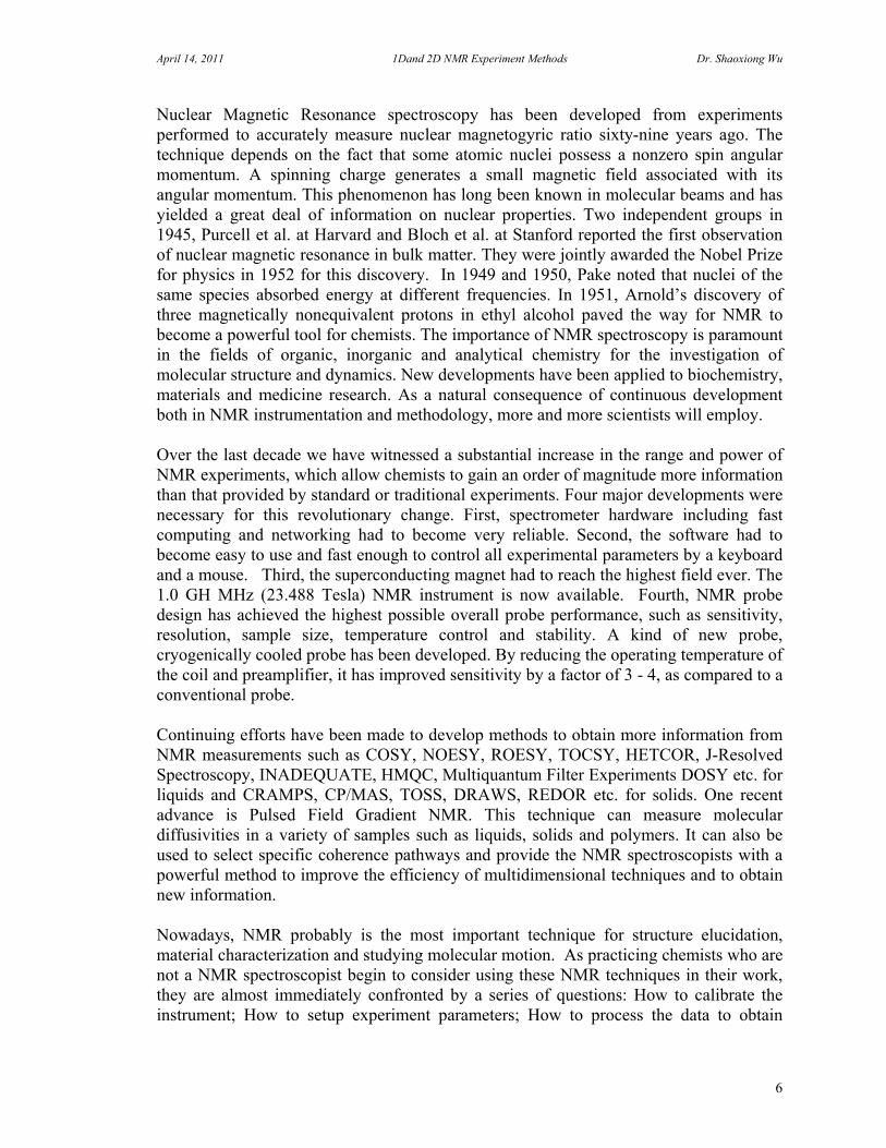
Where is the magnetogyric ratio, and B0 is the strength of the magnetic field. NMR spectra are typically in the range 10 – 900 MHz, corresponding to wavelengths from 30 meter down to 40 center meter. This is the radiofrequency (RF) part of the electromagnetic spectrum which is used for radio, TV and cell phones. If a magnetic field B1 (typical strength 7.04 10-4 T) is placed along the X axis, a 90 degree pulse width can be calculated by:
HzTSTB
312492
1034.71075.26
2
41171
1
A 90 degree pulse width = s831249
1
4
1
Figure 2 – 4. A 90 degree flip of a spin under magnetic field B1 along the X axis. C. Spin-Lattice and Spin-Spin Relaxation When a sample is inserted into the magnetic field B0, the Boltzmann distribution of spins occurs between the energy levels. The equilibrium is established by means of specific relaxation process and gives rise to a small excess of nuclei in the lower state. We can apply an oscillating field, B1 perpendicular to the B0 axis, to manipulate this spin system. After B1 is removed, there are two different mechanisms that allow spins return to equilibrium of the longitudinal and transverse components. The spin-lattice relaxation is a process whereby non-radiative energy transfer takes place from “excited” spins to the surrounding of the molecules. These relaxation processes can be described by the Bloch equations:
X
Y
Z
B0
X '
Y '
Z
B1

April 14, 2011 1Dand 2D NMR Experiment Methods Dr. Shaoxiong Wu
11
M
tM H
M M
Tz
zz
( ) 0
1
(2 – 6)
M
tM H
M
Tx
xx ( )
2
(2 – 7)
M
tM H
M
Ty
yy ( )
2
(2 – 8)
Where T1 is the spin-lattice relaxation time and T2 is the spin-spin relaxation time. The magnitude of T1 and T2 is related to the relaxation efficiency that is a property of the molecule. T1 and T2 are also related to the structure and mobility of the molecule. D. Chemical Shift When an atom is placed in a magnetic field, its electrons circulate about the direction of the applied magnetic field. This circulation causes a small magnetic field at the nucleus that opposes the externally applied field. Figure 2 – 5. A water molecule is placed in a magnetic field. Its electrons cause a small magnetic field that opposes the applied filed. The magnetic field at the nucleus (the effective field) is therefore generally less than the applied field by a fraction (parts per million or ppm). B = Bo (1-) (2 – 9) So the Larmor frequency of the nucleus under observation is a little smaller than =B. We use TMS as a chemical standard, its frequency under the field refer to =Bo, or fref. In an NMR spectrum, each nucleus has a characteristic frequency or chemical shift. It is defined as:

April 14, 2011 1Dand 2D NMR Experiment Methods Dr. Shaoxiong Wu
12
ppmref
ref ref
f f
f
f Hz
f MHz
106 ( )
( ) (2 – 10)
It is usual in spectroscopy to quote the frequency or wavelength of the observed adsorptions, in contrast, in NMR we give the position of the peaks in ppm, since the frequencies of the peak are directly proportional to the magnetic field strength. The peak position in Hz. is magnetic field dependent. For proton NMR, one peak at 500 Hz from the TMS peak under the static field of 11.74 Tesla (500MHz NMR instrument). However, under the static field of 4.70 Tesla (200 MHz NMR instrument), this peak will be at 200 Hz from TMS. The magnetic field dependence makes it difficult to compare peaks frequencies between spectrometers that operate at different field strength. It is to get round this problem that chemical shit scale is introduced. On this scale, the positions of the peaks are independent of the field strength. From the above sample, the peak is at 1 ppm from TMS peak for both instruments (1ppm = 500 Hz under the field of 11.74 T, and 1 ppm = 200 Hz under the field of 4.74 T). The chemical shift is a finger printer of a nucleus in the molecule. It relates to nucleus’s environment and relative position in the molecule. However, the J coupling relates to the interaction between nuclei, it is magnetic field independent. If a proton signal is coupled with another proton with J coupling constant 10 Hz. This number will not change under different magnetic fields.
60MHZ
200MHZ
500MHZ
J J
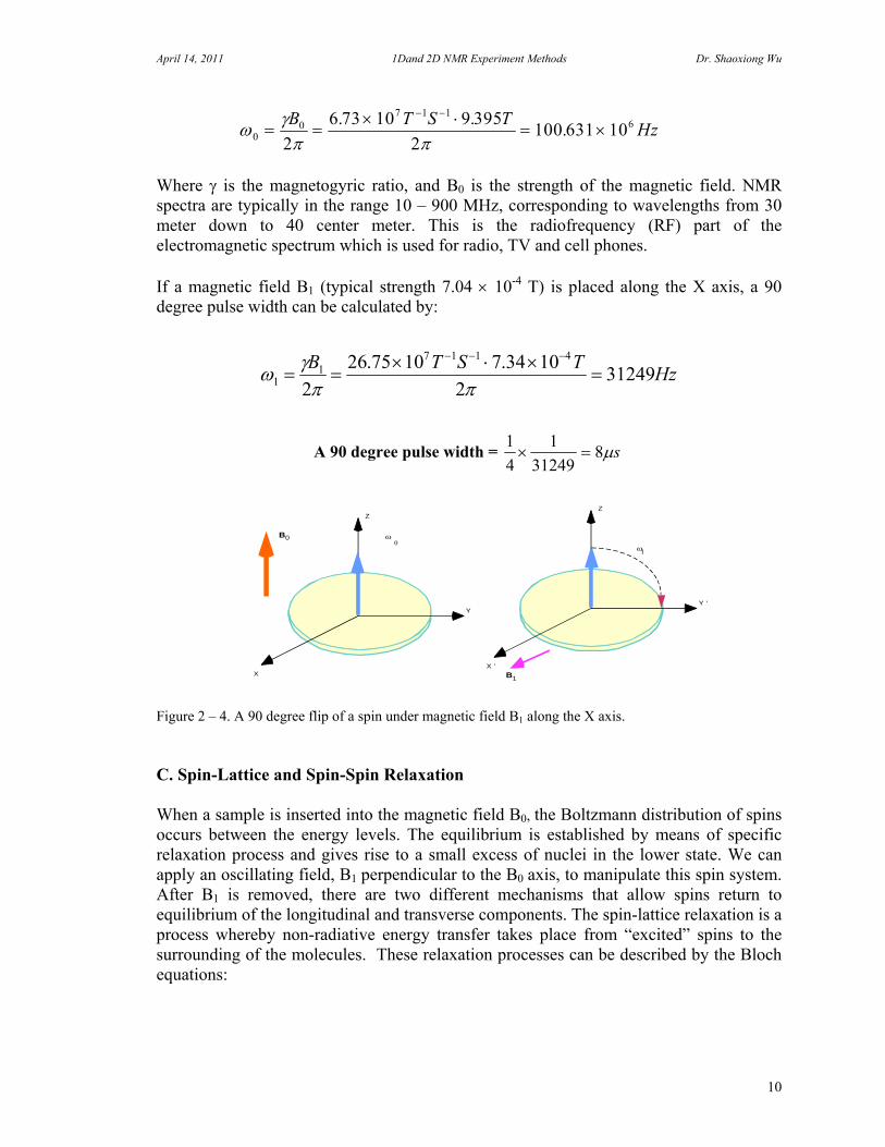
Figure 2 - 6. Two spins coupled each other with a coupling constant J. The chemical shift , 1ppm is equal to 60, 200 and 500 Hz respect to the static field of 60, 200 and 500 MHz instruments. The J is a constant in different field, however, Chemical shift between peaks (in Hz) is increased as field strength increasing, so the two pair of peaks will be resolved in a spectrum acquired in a high field while overlapped in lower filed.
April 14, 2011 1Dand 2D NMR Experiment Methods Dr. Shaoxiong Wu
13
Figure 2 – 7. Part of proton spectrum of Strychnine in CDCl3. From the top: 300 MHz, 400 MHz and 600 MHz. The J couplings in Hz are the same, but the chemical shifts are separated more in a high field. Chemical shifts arise from the simultaneous interaction of a nucleus with an electron and the electron with the applied static magnetic field. It is practically impossible to calculate a chemical shift value from the screening factor due to the complexity of the mechanisms that give rise to it. Also the chemical shifts are solvent and temperature dependent. Even though, there are still people using software to predict an NMR spectrum from a molecule structure, since calculated NMR spectrum could give us the relative chemical shifts. E. Spin-Spin Coupling (Scalar Coupling or J-Coupling) Spin-Spin coupling is the interaction of spins through the bonding electrons. It results in the multiple peaks observed in the NMR spectra. The distance (ALWAYS in Hz) between the multiple peaks (JH-H or JH-X) provides important molecular structure information. If two protons are magnetically inequivalent, there are two peaks in the spectrum for each proton. If these two protons are scalar coupled, then one senses the spin states of the other. Since proton (I=1/2) has two energy levels (+1/2, -1/2), the coupled protons will be split to two lines relative to the two energy states. If one of the nuclei has a spin of
4 . 4 4 . 3 4 . 2 4 . 1 4 . 0 3 . 9 3 . 8 3 . 7 P P M
4 . 4 4 . 3 4 . 2 4 . 1 4 . 0 3 . 9 3 . 8 3 . 7 P P M
4 . 4 4 . 3 4 . 2 4 . 1 4 . 0 3 . 9 3 . 8 3 . 7 P P M

April 14, 2011 1Dand 2D NMR Experiment Methods Dr. Shaoxiong Wu
14
one (I=1), then the nucleus to which it is coupled become split into three lines because the nucleus has three energy levels (+1, 0, -1). A good example is CDCl3, the carbon spectrum will have a triplet with equivalent intensity since deuterium has spin of one (I=1).
Figure 2 – 8. (A). Proton a and b are not coupled. (B). Proton a and b are coupled. (C). Carbon is coupled with D (I=1) and the carbon spectrum will be a triplet. Confusion can arise as the term strong coupling is sometimes used to mean a coupling constant with a large size (in Hz). Strictly this is an erroneous us of the term. The strong coupling, in contrast, is that the frequency separation of the peaks from two coupled spins is comparable to the coupling constant between them. In this case, both the frequencies and intensities of four peaks (two doublets for two coupled protons) are perturbed from the week coupling. In most case, the outer peaks become shorter and the inner peaks become higher. This intensity perturbation is usually called “roofing”. F. Dipole-Dipole Coupling Dipole-Dipole coupling is the coupling of spins through the space. They could be bonded but not necessary bonded, as long as they are close enough in the space. The Dipole-Dipole interaction is an important source of relaxation effect, but not necessary broaden the lines in liquids. In solids, however, it is the dominant source of line broadening. If there are two spins, I and S, an approximate dipolar Hamiltonian can be written as:
Hr
I S I Sd dI S
z z 1
21 3 3
2
32
( cos )( ) (2 – 11)
Where is the angle between the inter-nuclear vector and the applied field, r is the distance between two nuclei. In liquid, due to the random motion of molecules, is a random value. The average value of (1-3cos2) is zero for all possible directions. For some liquid samples, the average value of (1-3cos2) may not be zero, since the molecule is very large or very viscous solvent, or at low temperature, broad peaks may be observed. In solids, the value of (1-3cos2) is not zero since molecule cannot move
C
H
C
Ha
a
b
b
(A)
C
H
C
Ha
a
b
b
(B)
C
D
(C)

April 14, 2011 1Dand 2D NMR Experiment Methods Dr. Shaoxiong Wu
15
freely. Hd-d is the major line-broadening factor (in KHz). In order to narrowing the line, the CP/MAS (Cross Polarization/ Magic Angle Spinning) probe is designed so that the angle between sample tube and field is 54.7 degree. The term (1-3cos2) in the equation will be zero when is equal to 54.70 and sample is spinning in few KHz. (Refer to Magic Angle Spinning Experiments). G. Cross Polarization (CP) The presence of strong dipole coupling between rare spin (such as 13C) and abundant spin (such as 1H) in solids or the presence of scalar J coupling (JC-H) in liquids can be used to enhance the sensitivity of the rare spin observation under an appropriate conditions. Cross Polarization or Polarization Transfer is very important technique to observe chemical shift correlation between two different nuclei, to observe very insensitive nuclei coupled to proton, such as 15N. The key to this type of experiments (DEPT, INEPT) are that the signal of the nucleus that we observe in somehow modulated by the chemical shift of one or more other nuclei through the polarization transfer. H. Nuclear Overhauser Effect (NOE) A change in the integrated NMR absorption intensity of a spin when the NMR absorption of another nearby spin is saturated is known as the Nuclear Overhauser Effect (NOE). It is field and mobility dependent in solution of the molecule under study. The NOE is a very important tool for determination of the distance between spins. However, the interpretation of NOE measurement, i.e. a steady-state measurement or transient protocol measurement; requires more care than for those methods that measurement of scalar couplings. The steady-state NOE measurement that is pre-saturation or NOE difference experiments is for small molecule under 1000, or molecule in rapidly motion or in non-viscous solvent. The transient NOE measurement that is 2D NOESY is suitable for molecule smaller than 1000 (NOE is positive) and larger than 2000 (NOE is negative). For midsize molecules (1000 – 2000) may fail. It is here that the ROESY may be employed for those molecules. The NOE is characterized by an enhancement factor:
N O E
I I
I
0
0
(2 – 12)
Where I0 is the intensity of a peak without irradiation of the other spins, and the I with irradiation. The intensity changes brought about by the NOE can be both positive (an increase intensity) or negative (a decrease intensity) as dictated by the motional
April 14, 2011 1Dand 2D NMR Experiment Methods Dr. Shaoxiong Wu
16
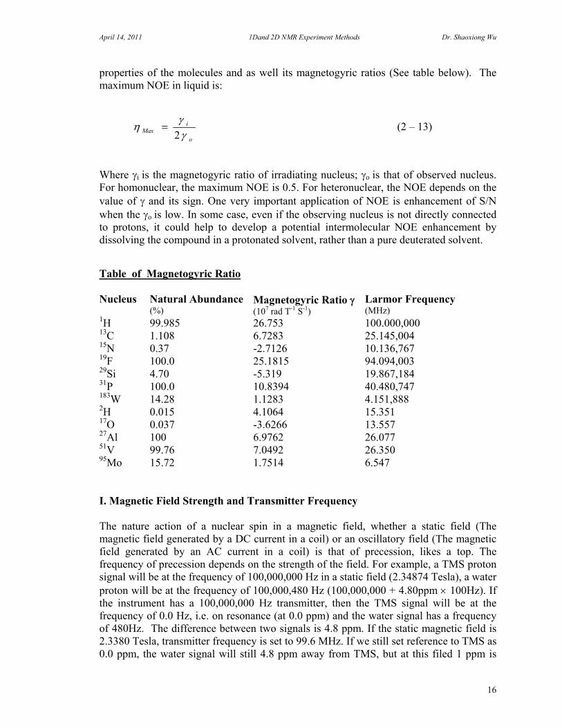
properties of the molecules and as well its magnetogyric ratios (See table below). The maximum NOE in liquid is:
o
iMax
2
(2 – 13)
Where i is the magnetogyric ratio of irradiating nucleus; o is that of observed nucleus. For homonuclear, the maximum NOE is 0.5. For heteronuclear, the NOE depends on the value of and its sign. One very important application of NOE is enhancement of S/N when the o is low. In some case, even if the observing nucleus is not directly connected to protons, it could help to develop a potential intermolecular NOE enhancement by dissolving the compound in a protonated solvent, rather than a pure deuterated solvent. Table of Magnetogyric Ratio Nucleus Natural Abundance
(%) Magnetogyric Ratio (107 rad T-1 S-1)
Larmor Frequency (MHz)
1H 99.985 26.753 100.000,000 13C 1.108 6.7283 25.145,004 15N 0.37 -2.7126 10.136,767 19F 100.0 25.1815 94.094,003 29Si 4.70 -5.319 19.867,184 31P 100.0 10.8394 40.480,747 183W 14.28 1.1283 4.151,888 2H 0.015 4.1064 15.351 17O 0.037 -3.6266 13.557 27Al 100 6.9762 26.077 51V 99.76 7.0492 26.350 95Mo 15.72 1.7514 6.547 I. Magnetic Field Strength and Transmitter Frequency The nature action of a nuclear spin in a magnetic field, whether a static field (The magnetic field generated by a DC current in a coil) or an oscillatory field (The magnetic field generated by an AC current in a coil) is that of precession, likes a top. The frequency of precession depends on the strength of the field. For example, a TMS proton signal will be at the frequency of 100,000,000 Hz in a static field (2.34874 Tesla), a water proton will be at the frequency of 100,000,480 Hz (100,000,000 + 4.80ppm 100Hz). If the instrument has a 100,000,000 Hz transmitter, then the TMS signal will be at the frequency of 0.0 Hz, i.e. on resonance (at 0.0 ppm) and the water signal has a frequency of 480Hz. The difference between two signals is 4.8 ppm. If the static magnetic field is 2.3380 Tesla, transmitter frequency is set to 99.6 MHz. If we still set reference to TMS as 0.0 ppm, the water signal will still 4.8 ppm away from TMS, but at this filed 1 ppm is
April 14, 2011 1Dand 2D NMR Experiment Methods Dr. Shaoxiong Wu
17
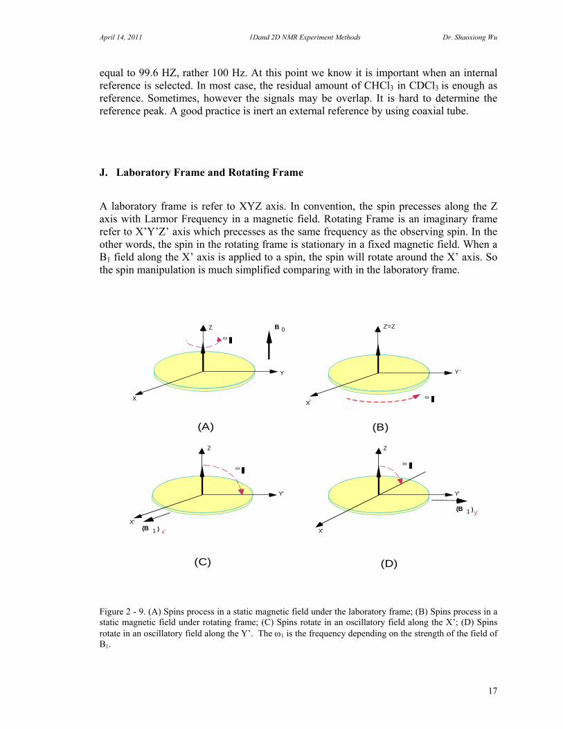
equal to 99.6 HZ, rather 100 Hz. At this point we know it is important when an internal reference is selected. In most case, the residual amount of CHCl3 in CDCl3 is enough as reference. Sometimes, however the signals may be overlap. It is hard to determine the reference peak. A good practice is inert an external reference by using coaxial tube. J. Laboratory Frame and Rotating Frame A laboratory frame is refer to XYZ axis. In convention, the spin precesses along the Z axis with Larmor Frequency in a magnetic field. Rotating Frame is an imaginary frame refer to X’Y’Z’ axis which precesses as the same frequency as the observing spin. In the other words, the spin in the rotating frame is stationary in a fixed magnetic field. When a B1 field along the X’ axis is applied to a spin, the spin will rotate around the X’ axis. So the spin manipulation is much simplified comparing with in the laboratory frame.
Figure 2 - 9. (A) Spins process in a static magnetic field under the laboratory frame; (B) Spins process in a static magnetic field under rotating frame; (C) Spins rotate in an oscillatory field along the X’; (D) Spins rotate in an oscillatory field along the Y’. The 1 is the frequency depending on the strength of the field of B1.
X
Y
Z
X'
Y'
Z
(B 1 )
(B 1 )
X
Y '
Z'=Z
'
(A) (B)
(C) (D)
B 0
X'
Y'
Z
x'
y'

April 14, 2011 1Dand 2D NMR Experiment Methods Dr. Shaoxiong Wu
18
3. Fundamentals of NMR Experiment A. Nuclei in an NMR Tube In liquids, molecules are free and the directions of spins are random. There is no net magnetization observable. If molecules are placed in a magnetic field, however, the spins are under the influence of the magnetic field and they will align along the field. A bulk magnetization will be generated. The bulk magnetization can be manipulated by pulses and observed.
Spins in an NMR tube Under a magnetic field Observable spins
Figure 3 – 1. Spins in an NMR tube. Under the magnetic field, spins “equilibrium magnetization” align
along the direction of magnetic field.
B. A 90 Degree Pulse In order to manipulate the bulk magnetization, a “controlled” electronic magnetic field B1 is used. The “controlled” means that we are able to turn on and off the magnetic field B1 by applying an RF pulse. In convention, the B1 is perpendicular to the main magnetic field B0. If the B1 is turned on, the spin vector will be rotated around X axis (Assume B1 is along the X axis). Until the spin vector turns to XY plane, the B1 can be turned off. The spin vector will be free to precess in the XY plane and will return to Z axis. The duration of applying the B1 to tip the spin vector through exactly 90 degree is called a 90 degree pulse. A 180 degree pulse will double the time of a 90 degree pulse. For a nucleus, the actual time to perform a 90 degree pulse is a function of the input RF power, coil efficiency and magnetic field strength. Usually a 90 degree pulse is determined by
April 14, 2011 1Dand 2D NMR Experiment Methods Dr. Shaoxiong Wu
19
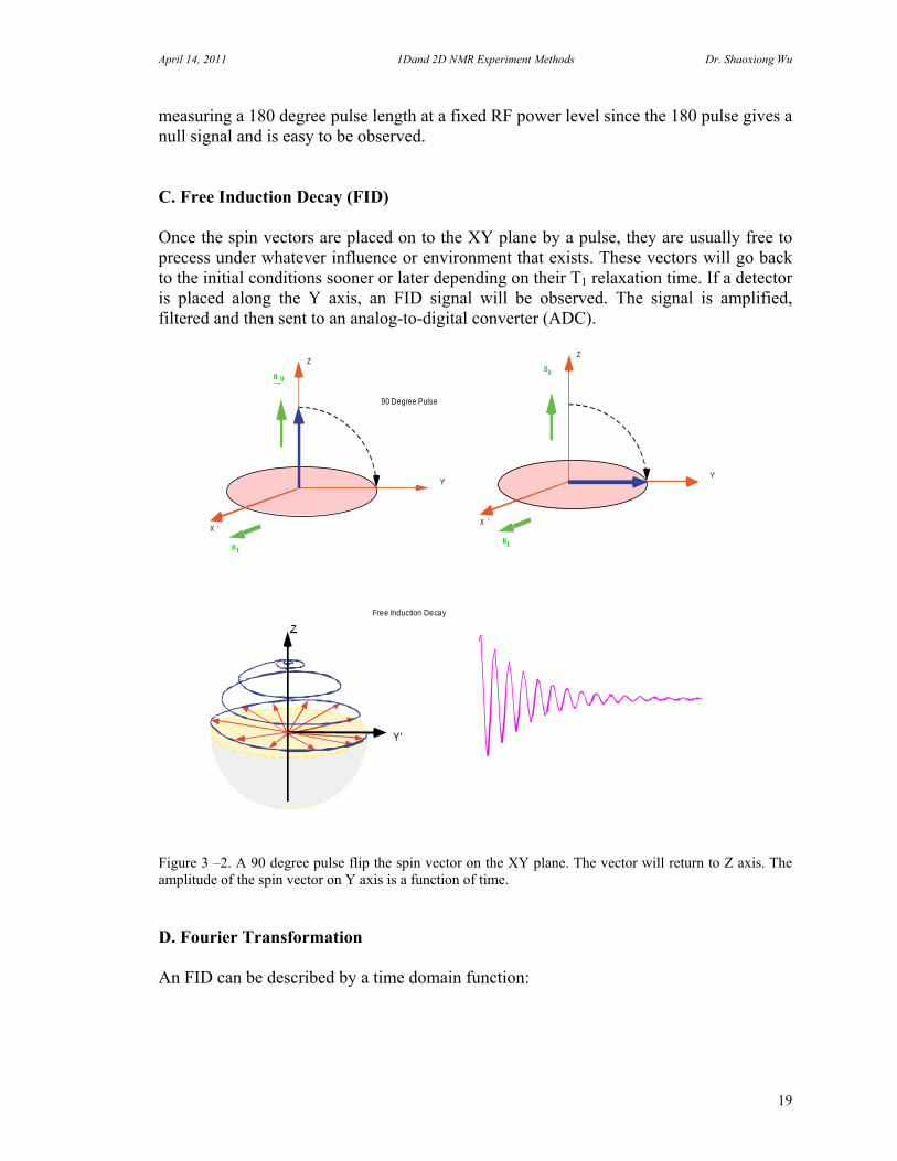
measuring a 180 degree pulse length at a fixed RF power level since the 180 pulse gives a null signal and is easy to be observed. C. Free Induction Decay (FID) Once the spin vectors are placed on to the XY plane by a pulse, they are usually free to precess under whatever influence or environment that exists. These vectors will go back to the initial conditions sooner or later depending on their T1 relaxation time. If a detector is placed along the Y axis, an FID signal will be observed. The signal is amplified, filtered and then sent to an analog-to-digital converter (ADC).
Figure 3 –2. A 90 degree pulse flip the spin vector on the XY plane. The vector will return to Z axis. The amplitude of the spin vector on Y axis is a function of time. D. Fourier Transformation An FID can be described by a time domain function:
Z
Y'
X '
0
B1
Z
Y'
X '
B0
B1
90 Degree Pulse
Free Induction Decay
B
Y'
April 14, 2011 1Dand 2D NMR Experiment Methods Dr. Shaoxiong Wu
20
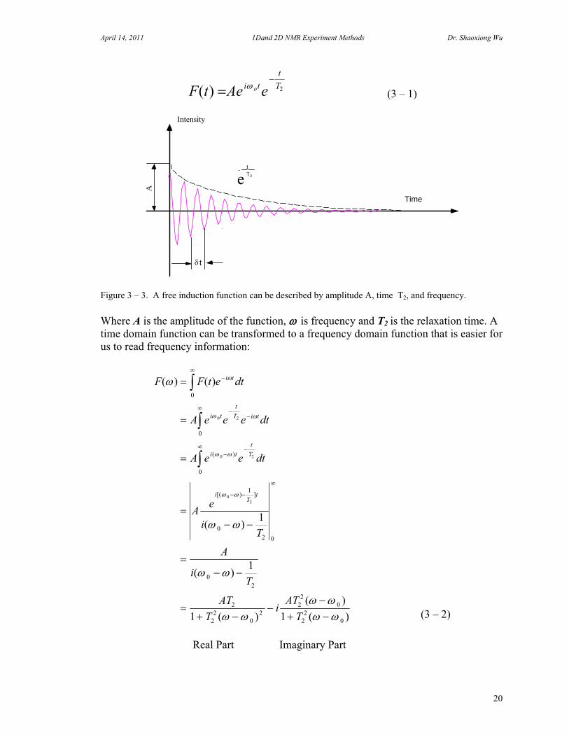
F t Ae ei t
t
To( )
2 (3 – 1)
Figure 3 – 3. A free induction function can be described by amplitude A, time T2, and frequency. Where A is the amplitude of the function, is frequency and T2 is the relaxation time. A time domain function can be transformed to a frequency domain function that is easier for us to read frequency information:
F F t e dt
A e e e dt
A e e dt
Ae
iT
A
iT
AT
Ti
AT
T
i t
i t
t
T i t
i t
t
T
iT
t
( ) ( )
( )
( )
( )
( )
( )
( )
[( ) ]
0
0
0
1
02 0
02
2
22
02
22
0
22
0
0 2
0 2
02
1
1
1 1 (3 – 2)
Real Part Imaginary Part
e1T2
-
Time
Intensity
A
t
April 14, 2011 1Dand 2D NMR Experiment Methods Dr. Shaoxiong Wu
21
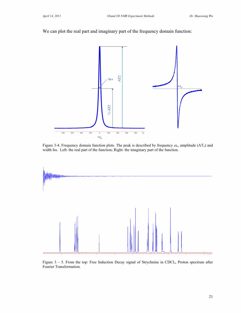
We can plot the real part and imaginary part of the frequency domain function:
Figure 3-4. Frequency domain function plots. The peak is described by frequency o, amplitude (AT2) and width δω. Left: the real part of the function; Right: the imaginary part of the function.
Figure 3 – 5. From the top: Free Induction Decay signal of Strychnine in CDCl3, Proton spectrum after Fourier Transformation.
800 600 400 200 0 -200 -400 -600 -800 Hz
AT2
½ A
T2
8 7 6 5 4 3 2 1 0 P P M

April 14, 2011 1Dand 2D NMR Experiment Methods Dr. Shaoxiong Wu
22
E. Base Line Correction and Weight Functions The finite impulse response time of the receiver is the main reason of NMR spectral baseline distortion. The degree of distortion is related to the receiver gate speed, spectral width, finite acquisition times and Q factor of the observe coil. A general method to correct the base line distortion is the cubic spine technique. The selected baseline data points are automatically to fit to cubic polynomials with the constraint. Base line correction has been implemented into most of NMR processing software. Weight Functions (WF) or Window Functions are applied to an FID prior to Fourier Transformation for enhancing the signal intensity or increasing the resolution. Use of WF is an essential part of the process of analyzing a spectrum. F. Data Points, Spectral Width and Digital Resolution The highest frequency to be recorded by digitizing at a particular rate is known as the Nyquist Frequency. In general, it is called Spectral Width (SW) in Hz. The minimum digitizing speed required for a desired SW is:
DigitizeRateSW
1
2 (3 – 3)
For a high resolution NMR instrument, the shortest ADC conversion time is typically in the range of 10s to 0.5s, giving maximum spectral widths from 100 kHz to 2MHz. Before we set up the ADC to digitize the FID signal, we need to decide the minimum resolution required for the spectrum. Suppose we desire a 0.2Hz resolution for a proton experiment. The minimum acquisition time is 5 seconds. The spectral resolution is defined by:
AtsR 1)( (3 – 4)
Where R(s) is in Hz. At is the acquisition time in seconds. In this case, the minimum acquisition time is 5 seconds. If a normal spectral width of a proton spectrum is 5000 Hz on a 500 MHz instrument. The digitization speed is 1/(25000) = 100s. The total data points are 5/0.0001 = 50,000. The digital resolution is defined by:
np
SWdR
2
)( (3 – 5)
Where R(d) is in Hz per point, sw is the spectral width and np is the total data points. Some old instruments may only have a maximum data of 32k points. In order to have the same resolution, you have to decrease the spectral width.
April 14, 2011 1Dand 2D NMR Experiment Methods Dr. Shaoxiong Wu
23
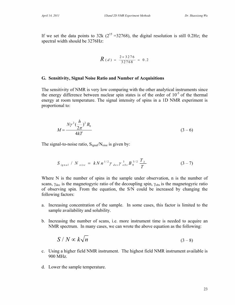
If we set the data points to 32k (215 =32768), the digital resolution is still 0.2Hz; the spectral width should be 3276Hz:
R d( ) .
2 3 2 7 6
3 2 7 6 80 2
G. Sensitivity, Signal Noise Ratio and Number of Acquisitions The sensitivity of NMR is very low comparing with the other analytical instruments since the energy difference between nuclear spin states is of the order of 10-5 of the thermal energy at room temperature. The signal intensity of spins in a 1D NMR experiment is proportional to:
MN
hB
kT
2 202
4
( ) (3 – 6)
The signal-to-noise ratio, Signal/Noise is given by:
S N k N n BT
Tig n a l o i s e d e c o b s/ / / 1 2 303 2 2 (3 – 7)
Where N is the number of spins in the sample under observation, n is the number of scans, dec is the magnetogyric ratio of the decoupling spin, obs is the magnetogyric ratio of observing spin. From the equation, the S/N could be increased by changing the following factors: a. Increasing concentration of the sample. In some cases, this factor is limited to the
sample availability and solubility. b. Increasing the number of scans, i.e. more instrument time is needed to acquire an
NMR spectrum. In many cases, we can wrote the above equation as the following:
S N k n/ (3 – 8) c. Using a higher field NMR instrument. The highest field NMR instrument available is
900 MHz. d. Lower the sample temperature.
April 14, 2011 1Dand 2D NMR Experiment Methods Dr. Shaoxiong Wu
24
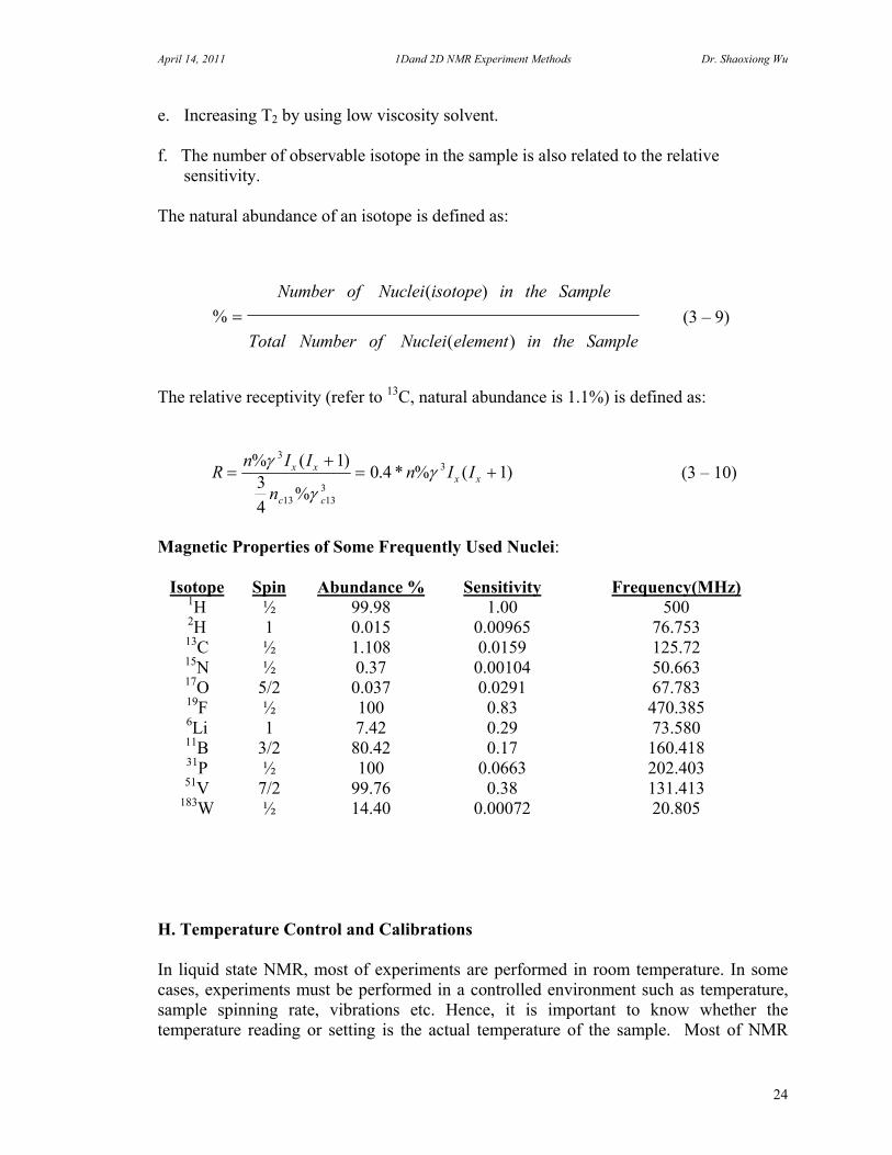
e. Increasing T2 by using low viscosity solvent. f. The number of observable isotope in the sample is also related to the relative sensitivity. The natural abundance of an isotope is defined as:
%
( )
( )
Number of Nuclei isotope in the Sample
Total Number of Nuclei element in the Sample (3 – 9)
The relative receptivity (refer to 13C, natural abundance is 1.1%) is defined as:
Rn I I
nn I Ix x
c c
x x
% ( )
%.4 * % ( )
3
13 133
313
4
0 1 (3 – 10)
Magnetic Properties of Some Frequently Used Nuclei:
Isotope Spin Abundance % Sensitivity Frequency(MHz) 1H ½ 99.98 1.00 500 2H 1 0.015 0.00965 76.753 13C ½ 1.108 0.0159 125.72 15N ½ 0.37 0.00104 50.663 17O 5/2 0.037 0.0291 67.783 19F ½ 100 0.83 470.385 6Li 1 7.42 0.29 73.580 11B 3/2 80.42 0.17 160.418 31P ½ 100 0.0663 202.403 51V 7/2 99.76 0.38 131.413
183W ½ 14.40 0.00072 20.805 H. Temperature Control and Calibrations In liquid state NMR, most of experiments are performed in room temperature. In some cases, experiments must be performed in a controlled environment such as temperature, sample spinning rate, vibrations etc. Hence, it is important to know whether the temperature reading or setting is the actual temperature of the sample. Most of NMR

April 14, 2011 1Dand 2D NMR Experiment Methods Dr. Shaoxiong Wu
25
instruments are equipped with a VT unit (Variable Temperature Control Units). It includes an Air/N2 gas supply, temperature monitor and cooling unit. The heater and thermal couple are built in the probe. In the high field NMR instrument, a temperature sensor in the probe measures the sample temperature. It is necessary to use another mean to check if it is accurate. There are many ways to calibrate the temperature. A well known method is the measurement of the chemical shifts of –OH to CH3 of methanol for low temperature calibration, 1,2-ethanediol for high temperature calibration, since as the temperature rises the amount of hydrogen bonding diminishes, and the OH proton resonance moves upfield toward the CH3 resonance. According to the chemical shift difference between two peaks, we can calculate the relative temperature of the sample in the probe.
T ( ) .4 8 ( ) . ( )0 24 0 3 2 9 2 3 8 1K p p m p p m (3 – 11) Where is the chemical shifts difference between two proton peaks in ppm. If the experiment temperature is below 5 oC or higher than 100 oC, the N2 gas should be used for temperature control. The chiller is capable of cooling down the input N2 gas to -80 oC, the lowest temperature of sample is about -45 oC because of the heat loss in the transfer line. If lower temperature is required, a low-temperature bath may be used to cool down the VT N2 gas.
Cryogen System Operation Temperature
(oC) (oK) Methanol/Liquid Nitrogen -98 175 Cyclohexene/ Liquid Nitrogen -104 169 Methyl Cyclohexane/ Liquid Nitrogen -126 147 1,5-Hexadiene/ Liquid Nitrogen -141 132 Liquid Nitrogen -196 77
Note: The boiling point of liquid oxygen is 90 oK (-183 oC), it is higher than that of liquid nitrogen, i.e. oxygen will be liquefied at -183 oC while the liquid nitrogen temperature is -196 oC. If liquid nitrogen is used for cryogen, before the VT system can be switched from nitrogen gas to regular air, all system should be warmed up to room temperature.

April 14, 2011 1Dand 2D NMR Experiment Methods Dr. Shaoxiong Wu
26
Air
Air Filter
Air/N2 Switch
LN2 Tank
N2 Gas
VT Control Unit
25 C
C o m p u te r
C h il le r
C o il
Thermal Couple
He at er
VT Cable
S a m p le
Figure 3 – 6. A typical cooling/heating system for VT operation. The chiller can be replaced by a cryogen dewar flask with a heat exchange coil.
April 14, 2011 1Dand 2D NMR Experiment Methods Dr. Shaoxiong Wu
27
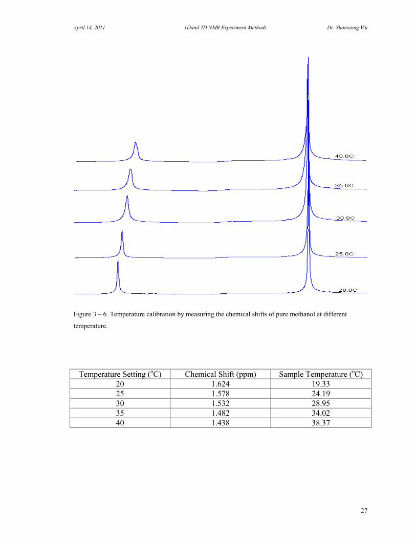
Figure 3 – 6. Temperature calibration by measuring the chemical shifts of pure methanol at different
temperature.
Temperature Setting (oC) Chemical Shift (ppm) Sample Temperature (oC) 20 1.624 19.33 25 1.578 24.19 30 1.532 28.95 35 1.482 34.02 40 1.438 38.37

April 14, 2011 1Dand 2D NMR Experiment Methods Dr. Shaoxiong Wu
28
4. NMR Probes and Tuning A. Probes and Their Functions NMR probe is the most delicate part of the instrument. Shimming, sensitivity, baseline and pulse width are important specifications of a probe. In general, manufacture provides a list of specifications such as line shape, line width, 90 degree pulse width, tunable frequency range, operation temperature range and sensitivity. The 90 degree pulse width, sensitivity and shims should be routinely checked. If the results of these checks are religiously recorded in an instrument logbook, then gradual degradation is more easily detectable. When deciding between different probes, it is helpful to identify the observe nuclei in your samples that require the greatest sensitivity so that you can choose the most appropriate probe family for your work. The range of price for a probe is from $18,000 to $64,000 each. One probe can provide a high quality spectrum while the other may be not on a same instrument. In order to meet special experiment requirements, there are several types of probes. For liquid NMR applications: Broad band probe, Four Nuclei probe, Indirect Detection (ID) probe, Auto-Tune probe, Triple resonance probe, CryoProbe etc.. For solid state NMR applications: CP/MAS probe, Triple resonance probe, HFX probe, HRMAS probe etc.. Each kind of probe has been designed to meet experimental specific applications.
Figure 4 – 1. Left: Varian 600 MHz probe. Right: GE Broad Band probe, the DT and DM are decoupling tune and match, the OT and OM are Observe tune and match. The LT and LM are lock tune and match.
Sample
Obs Lock Dec Body Air
LM LT
DT
DM O
TO
M
Bottom View of a Probe
Spiner
RF Coil
Thermal Couple
Vacuum Tube
Heater
VT Air/N2 Input
VT Cable

April 14, 2011 1Dand 2D NMR Experiment Methods Dr. Shaoxiong Wu
29
Four nuclei probe (1H, 19F/13C, 31P) is a very popular probe in routine NMR applications. It provides automated four nuclei capability for laboratories that require high sample through put without the need for the user to adjust the probe. Nuclei change is automatic without mechanical switching. The probe is designed with a 13C and 31P simultaneously tuned inner coil for optimum sensitivity and simultaneously tuned 1H and 19 F, as well we 2H outer coil. The four nuclei probe can be used for single, double, and triple resonance experiments.
Indirect detection probe (1H {15N – 31P}) offers very high 1H sensitivity for inverse detected experiments and have the capability for decoupling over the broadband frequency range. The inner coil is tuned to 1H or tunable from 1H - 19F (depending on probe model), and outer coil is tunable over the frequency range (15N - 31P).
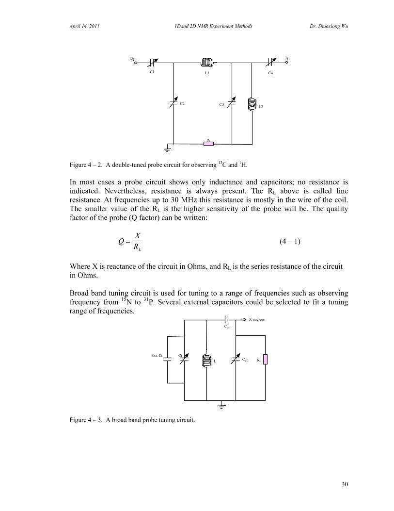
The specifications of a probe are very important. The following test should be done by an NMR specialist: a) line shape and resolution; b) 1H, 15N and 31P sensitivity tests, c) 90 degree pulse width; d) home- and heteronuclear nuclear decoupling range and efficiency; e) VT operation range and stability, f) gradient capability and stability. These data should be kept in the log book. B. Probe Tuning: The probe must be tuned to the observe frequency with the particular sample of interest. There can be a big difference depending on the solvents and concentration, such as water or organic solvents. When the probe is tuned the power is efficiently transferred from the transmitter to the probe, rather than reflect back to the transmitter, and pulse width is minimized. On the other hand, the detected signal power is efficiently transferred to the preamplifier and the S/N ratio is maximized. Probe tuning is essential for obtaining a good spectrum, and for some advanced experiments to get any meaningful results at all. For most of solid state NMR experiments, the probe must be properly tuned at each time, otherwise high power could not efficiently delivered to the probe. It may cause arching or damage the probe. Although probe designs are different according to their functions, one has in general two adjustable capacitors. One is called tune and the other called match. The tune capacitor is used to adjust probe circuit to the desired frequency, most broad band probe have additional fixed external capacitors to extend the tune range. The match capacitor is used to adjust probe circuit to meet impedance requirement (50 Ohm). In most case, these capacitors are mutually interactive and therefore we should adjust them in turn. In general a Double-tuned probe circuit is used for a dual nucleus probe. The L1 is the center coil and L2 is the outer coil. The C1 and C4 are matching capacitors, and C2 and C3 are tuning capacitors. After the probe is tuned properly, the probe can be used to observe two nuclei at different frequency, or observe one nucleus while decoupling the other.
April 14, 2011 1Dand 2D NMR Experiment Methods Dr. Shaoxiong Wu
30
Figure 4 – 2. A double-tuned probe circuit for observing 13C and 1H. In most cases a probe circuit shows only inductance and capacitors; no resistance is indicated. Nevertheless, resistance is always present. The RL above is called line resistance. At frequencies up to 30 MHz this resistance is mostly in the wire of the coil. The smaller value of the RL is the higher sensitivity of the probe will be. The quality factor of the probe (Q factor) can be written:
QX
RL
(4 – 1)
Where X is reactance of the circuit in Ohms, and RL is the series resistance of the circuit in Ohms. Broad band tuning circuit is used for tuning to a range of frequencies such as observing frequency from 15N to 31P. Several external capacitors could be selected to fit a tuning range of frequencies.
Figure 4 – 3. A broad band probe tuning circuit.
13C
C1
C2 C3
L1
L2
C4
1H
RL
Cm2
Ct
L
Cm1
X nucleus
RL
Ext. Ct

April 14, 2011 1Dand 2D NMR Experiment Methods Dr. Shaoxiong Wu
31
Tune the probe with an Agilent 8712ET Network Analyzer This is the easiest way to tune a probe. You have to find a BNC to N-type adapter for Varian probe. Use FREQ to set tune frequency range. Use Marker to set the tune frequency. Use Tune and Match knobs to move the peak, until it is tuned.
Figure 4 -4. A tune signal on the display of Agilent 8712ET. Probe Tune for INOVA400 and UNITY400 After setup parameters for observing nucleus, connect probe to the tune port. Change the Channel switch to “1”, set the attenuator to “7”. Adjust tune and match knobs to minimize the number on the tune display. A tuned probe should be less than 10 on the tune display with attenuator set to “9”. After the probe is tuned, the channel switch should be set to “0”, and re-connect the cable back to the probe interface.
Figure 4 – 9. Varian INOVA400 Probe Tuning interface.

April 14, 2011 1Dand 2D NMR Experiment Methods Dr. Shaoxiong Wu
32
Probe Tune for Bruker Avance System: It is very easy to tune a probe on Bruker system. After a WOBB command issued, the computer will automatically setup to the tuning frequencies. A peak will be displayed on the screen. Also the tuning signal is displayed on the probe interface.
Figure 4 – 10. Bruker probe tuning interface and tuning signal. Probe Tuning Tips: If the previous tuned frequency is far from the frequency needs to be tuned to. First set the tune frequency about 20Mhz off the previous tuned frequency, using the tune knob to tune and to watch the tuning signal moving direction. Then set the tune frequency more towards to the tune frequency. In some cases, after insert the external capacitor, the tune signal disappears. You may have to increase the tune frequency window to see the tune signal. Do not connect any filters into the tuning circuit. C. Solid State NMR Probes High resolution solid state NMR requires fast sample spinning (up to 35 KHz) at the magic angle. It requires bearing air for supporting the rotor, and driving air to push the rotor spin, as well as temperature sensors and spin rate sensor. The angle of axis of the RF coil with magnetic field Bo is 54.44 degree. Because of homonuclear and heteronuclear dipole coupling, large decoupling power is required (~1000 Watts). Also there is only one RF coil that allows to tune to different frequencies. Most of solid state NMR probes have no lock circuit built in, since superconducting magnet is stable enough for most solid state NMR experiments.

April 14, 2011 1Dand 2D NMR Experiment Methods Dr. Shaoxiong Wu
33
Figure 4 – 11. From top left: Bruker 4 mm HFX solid state NMR probe base, bottom of the probe; probe head for wide bore magnet; Spinning test station; 4 mm solid sate NMR sample rotor.

April 14, 2011 1Dand 2D NMR Experiment Methods Dr. Shaoxiong Wu
34
5. The Art of Shimming A. The Magnetic Field and Cryogen Shims Most NMR instruments uses superconducting magnet. After the magnet is energized, its magnetic field is very stable. The drifting rate is under 5 Hz/per hour. All the superconducting magnets have build-in cryogen shims, these shims are adjusted by field service engineer when they energize the magnet. After the installation complete, these cryogen shims are no longer accessible.
Figure 5 -1. Across section of a superconducting magnet. The cryogen shims are built into superconductive solenoid. On the right; a room temperature shim coil. B. How the Sample and Probe Coil affect Shimming An NMR sample and its preparation have tremendous influence on the quality of the spectra and shim. The major effects: volume—End effects, materials in the sample, solvents and radiation damping: Volume and End Effects: All solvents have a very high magnetic susceptibility value, The NMR probe has an RF coil which is used to send and receive RF signals. The length of the RF coil is limited. The volume of the coil to hold samples is called active volume. As general rule, to avoid end effects of solvent the sample length should be longer than 1 cm above and below the active region. It is about 0.75 ml of a 5 mm NMR tube.
April 14, 2011 1Dand 2D NMR Experiment Methods Dr. Shaoxiong Wu
35
Particles --- Sample is not completely dissolved: The particles often have a very different magnetic susceptibility from its dissolved form. This influence on the magnetic homogeneity over active volume is very hard compensated by room temperature shims since these particles are moving, specially twhen the sample is spinning. Radiation Damping: A signal broadening phenomenon, which can be detected. Run a spectrum of the sample as the normal condition, and then measure the line width of the peak. Then de-tune the probe, i.e. tune the probe away of the resonance and the run the same sample at the same conditions. The peak will have less SN, but if the line width becomes narrower, then radiation damping is present. The sample will be very hard shim. C. Shims and Their Orders In early sixties when larger electromagnets were used for NMR instrument, the field homogeneity was adjusted by mechanical alignment of the magnet pole faces. By place thin pieces of brass between the magnet and the pole to make the poles more perfectly parallel. The metal pieces were called shim and the adjustment was called shimming. A well-shimmed electromagnet (1.4T) could yield line widths of 0.2 Hz. As the magnetic field is increased it is necessary to add electronic shimming which is a small coil placed around the probe. As the field become higher and higher, more and more shimming coils are added into the room temperature shimming coil, the shimming process become much more difficulty. The shims can be classified as the following gradient order: Zero Order: It is related to the field position in the magnet. The Z0 shim is the only zero order shim. First Order: The first order shims produce a small linear of magnetic field to overlap with the main magnetic field. There are three shims, Z1, X and Y. They should be adjusted first and last. Second Order: The second order shims produce a quadratic magnetic field to overlap with the main field and first order shims. There are five shims: Z2, ZX, ZY, XY and R2. After these shims adjusted, the first order shims should be readjusted. Third Order: The third order shims produce a cubic magnetic field to overlap with first order, second order shims. There are seven shims: Z3, Z2X, Z2Y, ZXY, ZR2, X3 and Y3. After these shims adjusted, the first order and second order shims should be readjusted. Fourth and Five Order: The fourth and fifth order shims produce a non-linear and composite function magnetic field to overlap with first order, second order and third order shims. There is only one-fourth-order shim, Z4 and one-fifth-order shim, Z5. After these two shims adjusted, Z3, Z2 and Z1 must be readjusted. A superconducting magnet typically contains 9 superconducting shimming coils and 17 room temperature shimming coils.

April 14, 2011 1Dand 2D NMR Experiment Methods Dr. Shaoxiong Wu
36
Superconducting Shims Room Temperature Shims Z0 Z1 Z2 Z0 Z1 Z2 Z3 Z4 Z5 Z6 Z7 X Y X Y ZX ZY XY ZX ZY Z2X Z2Y XY X2-Y2 X2-Y2 ZXY Z(X2-Y2) X3 Y3 Installation engineers normally adjusted the super-conducting shims. The room temperature shimming depends on magnet environment, probe, and tube type, solvent and sample volume. The first two facts are not much changed after installation. Adjusting shims can be performed in different ways, by observing the lock level, the FID shape and the area of the FID. The homogeneity can be checked by the line shape and resolution measurement. A good shimming can be done in minutes, but also could be done in several hour even days. An organized and logical approach can speed the process. An understanding of the shim interactions and their effect on the NMR signal will make the shimming easier. D. Raw Shimming If the instrument has a very poor homogeneity, the following steps are recommended. 1. Spin sample at rate 15-20 Hz. Adjust Z1 and Z2 to maximize the lock signal. Some
instruments may allow you to observe an FID signal. 2. Turn off the spinner. Adjust X and Y to maximize the lock signal. 3. Adjust X and ZX to maximize the lock signal. 4. Adjust Y and ZY to maximize the lock signal. 5. Adjust XY and X2 - Y2 to maximize the lock signal. 6. If a large signal intensity change observed, back to step 1. After these adjustments, the instrument should be able to lock. E. Spinning Shimming If the instrument have a fairly good shimming, but the line width is not good enough to provide good resolution. 1. Spin the sample at 15-20 Hz. Adjust Z1 and Z2 to maximize the signal.
April 14, 2011 1Dand 2D NMR Experiment Methods Dr. Shaoxiong Wu
37
2. Adjust Z3 (clockwise) to decrease the signal intensity about 20%, then adjust Z1 and Z2 to maximize the signal. Compare the signal intensities, if it is better, adjust Z3 more in the same direction, and then adjust Z1 and Z2 until reach to maximum. If it is worse, Adjust Z3 (anti-clockwise) to decrease the signal intensity about 20%, then adjust Z1 and Z2 again.
3. Adjust Z4 as same fashion as step 2. It may take much longer since after Z4 changed
the above step 1 and step 2 must be followed. 4. Adjust Z5. The best way is the same as above. F. None Spinning Shimming If the intensity of side band is larger than 1% of the main peak, this procedure is necessary. 1. Turn off the spinner. Adjust X and Y to maximize the lock signal. 2. Adjust ZX (clockwise) to decrease the signal intensity about 20%. Adjust X to
maximize the signal. If it is better, adjust ZX more in the same direction, if it becomes worse; adjust ZX in the other direction until signal maximized.
3. Adjust ZY (clockwise) to decrease the signal intensity about 20%. Adjust Y to
maximize the signal. 4. Interactively adjust XY and X2 -Y2. If the signal intensity changes lot, back to step 1,
2 and 3. If it does not change much, go to the next step. 5. Adjust Z2X (clockwise) to decrease the signal intensity about 20%. Adjust ZX and X
(see step 2) to maximize the signal. Compare the signal intensity, if it is better; adjust Z2X more in the same direction. If worse, adjust the Z2X in the other direction.
6. Adjust Z2Y with ZY and Y as the same way as step 5. 7. Adjust ZXY (clockwise) to decrease the signal intensity about 20%. Adjust XY to
maximize the signal. If it is better, adjust ZXY more, if it gets worse; adjust ZXY in the other direction.
8. Adjust Z(X2 -Y2) with X2 - Y2 as the same way as above. 9. Adjust X3 with X as the same way as above. 10. Adjust Y3 with Y as the same way as above. 11. If non-spin shims change lot, back to step D, repeat spinning shimming.

April 14, 2011 1Dand 2D NMR Experiment Methods Dr. Shaoxiong Wu
38
G. The Measurement of a Good Shim A good line shape is the most important feature for the performance of an NMR spectrometer. The line shape Measurement: Use a 1%CHCl3 in CDCl3 standard samples. Measure the line width at 50%, 0.55% and 0.11% of the peak height. A good NMR peak should be a Lorentzian line shape: 50% less than 0.3Hz 0.55% less than 13.5 0.3 = 4.05Hz 0.11% less than 30 0.3 = 9.00Hz The first order spin side band should be less than 1% of the main peak.
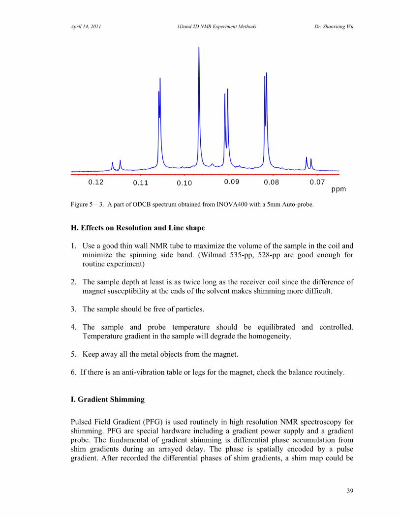
Figure 5 – 2. The spectrum shows the result obtained with a 5 mm Auto-probe 1H, 19F, 13C and 31P on INOVA400 spectrometer equipped with 14 room temperature shims. The line shape of the peak is 4.8\2.3\0.18 Hz relative to 0.11%\0.55%\50% of the height of the proton peak. The spin side bands are much smaller than the height of the 13C satellites. Resolution is the ability of an NMR spectrometer to observe resonance lines which are very close together as separate lines. The resolution measurement: Use a 5% Ortho-dichlorobenzene (ODCB) in Acetone_D6 standard sample. Usually the eighth line from the left is used for resolution measurement. The spectrum width should be set to 1ppm. The following spectrum shows the result obtained with a 5mm Auto-probe on INOVA400 spectrometer. The line-width at half-height measured on the eighth signal from the left was 0.1 Hz.
0.0 -0.1 -0.2 ppm0.10.20.3
April 14, 2011 1Dand 2D NMR Experiment Methods Dr. Shaoxiong Wu
39
Figure 5 – 3. A part of ODCB spectrum obtained from INOVA400 with a 5mm Auto-probe. H. Effects on Resolution and Line shape 1. Use a good thin wall NMR tube to maximize the volume of the sample in the coil and
minimize the spinning side band. (Wilmad 535-pp, 528-pp are good enough for routine experiment)
2. The sample depth at least is as twice long as the receiver coil since the difference of
magnet susceptibility at the ends of the solvent makes shimming more difficult. 3. The sample should be free of particles. 4. The sample and probe temperature should be equilibrated and controlled.
Temperature gradient in the sample will degrade the homogeneity. 5. Keep away all the metal objects from the magnet. 6. If there is an anti-vibration table or legs for the magnet, check the balance routinely.
I. Gradient Shimming
Pulsed Field Gradient (PFG) is used routinely in high resolution NMR spectroscopy for shimming. PFG are special hardware including a gradient power supply and a gradient probe. The fundamental of gradient shimming is differential phase accumulation from shim gradients during an arrayed delay. The phase is spatially encoded by a pulse gradient. After recorded the differential phases of shim gradients, a shim map could be
0.09 0.08 0.07ppm
0.100.110.12

April 14, 2011 1Dand 2D NMR Experiment Methods Dr. Shaoxiong Wu
40
calculated for a given shim set. Auto-Shimming can then be performed by constructing a background field map from the start shim values and fitting the result to the shim field maps. This allows iterative shimming with rapid convergence and excellent final results. The gradient shimming method uses a pair of gradient profile experiments to calculate the B0 filed homogeneity and then makes adjustment of Z gradient shims. So the first experiment is to map the shims.
Figure 5 -4. Shim map generated by using five shim gradients.
Figure 5 – 5. The red line is the gradient shim fit to a the shim map.
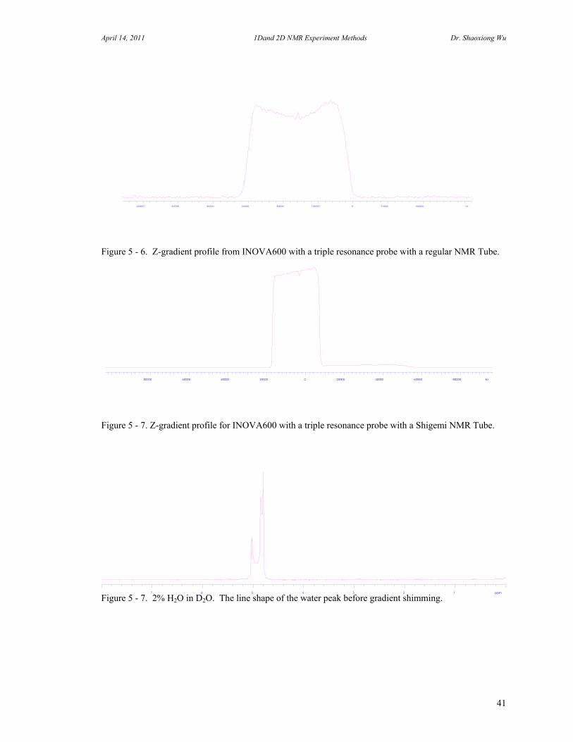
Use 20%H2O and 80% D2O standard sample. Adjust lock power, lock gain and lock phase for proper lock. Make coarse shim adjustments on Z1, Z2, X1 and Y1. Turn the spinner off.
April 14, 2011 1Dand 2D NMR Experiment Methods Dr. Shaoxiong Wu
41
Figure 5 - 6. Z-gradient profile from INOVA600 with a triple resonance probe with a regular NMR Tube.
Figure 5 - 7. Z-gradient profile for INOVA600 with a triple resonance probe with a Shigemi NMR Tube.
Figure 5 - 7. 2% H2O in D2O. The line shape of the water peak before gradient shimming.

April 14, 2011 1Dand 2D NMR Experiment Methods Dr. Shaoxiong Wu
42
Figure 5 - 8. 2% H2O in D2O. The line shape of the water peak after gradient shimming.
J. Shimming on Solid State NMR Probes In CPMAS experiments the spinner axis is at an angle 54.74 degree with the magnetic field direction and the distinction between the traditional spin and none-spin shims no longer holds. The spinning rates in solid state NMR experiments are typically a few kilohertz, which is much larger than the magnetic field in homogeneity. As a result the amplitudes of the sidebands are small, so none-spinning shims are ignored. We could use a set of shims that is cylindrically symmetric about the MAS spinner axis. These shims can be constructed from combinations of the standard laboratory frame shims, via a transformation to the tilted magic angle frame. In the simplest implementation the MAS probe is aligned such that the spinner axis is in the laboratory xz-plane or yz-plane. If we set the probe spinner axis in xz-plane, the MAS probe “Spinning z-shims” are X, ZX, Z2X, Z4 and Z5 (respectively to Z1 Z2 Z3 Z4 Z5 in liquid state NMR none-spinning shims). However, that the coefficients given for the magic angle shims do not take into account the efficiencies of the shim coils and the use of the other shims listed below may be needed.
MAS Shim Liquid State NMR Shims Z1
XZ3
2
3
1
Z2 ZXYX 22)( 22
Z3 22223
63
5)(
3
5
6
1
33
2XZYXXZZ

April 14, 2011 1Dand 2D NMR Experiment Methods Dr. Shaoxiong Wu
43
Z4 4
18
7Z
Z5 5
36
1Z
Table 5 -1. MAS spinning shims from combinations of the standard laboratory frame shims. If one of the shims requires an excessive shim current, reduce the current and continue shimming by adding current to another shim from the same group as shown in the table. For instance if the current in ZX is too high (Shimming on Z2 for MAS probe), reduce the value and optimize the line shape by adding current to the (X2-Y2) shim. If the probe is not exactly aligned with the xz plane then a small amount of Y and YZ may be needed for optimal shimming.

April 14, 2011 1Dand 2D NMR Experiment Methods Dr. Shaoxiong Wu
44
6. NMR Sample Preparation
If you could spend a few more minutes to prepare an NMR sample carefully, you may save hours of wasted instrument time. A good high resolution NMR spectrum can only be obtained on a completely particle free solution. In most case, filtering solution direct into the NMR tube is the best way to keep away from dust and insoluble materials. Never put NMR tubes in to oven! Since the tubes will change shape. If you need a dried NMR tube, put it into a clean desiccator or use nitrogen gas to dry it. There are lots tricks to prepare an NMR sample in different research area. You may consult with other experienced NMR users before you prepare an expensive sample. Here are some guidelines for preparing an NMR sample. A. Find a Good Deuterated Solvent Solvent Signals: Most NMR solvents are labeled with 99% of D or above, which means there still is about 1% proton in the solvent molecule. If your sample amount is comparable with the amount of proton in the solvent, the solvent peak will show up in the proton spectrum. In this case, the solvent peaks may overlap with the sample peaks. In some solvents, there is a water peak in the proton NMR spectrum. For example, water peak at 1.5 ppm in CDCl3 solvent and at 3.3ppm in DMSO solvent. Sometimes the water peak becomes very big because of bad solvent storage conditions. Keep your NMR solvent in a desiccator to prevent moisture and dust. Do not share NMR solvent with your peers. If your sample is crucial for the next reaction, use solvent in an ampoule that is only a few cents more. Solvent Viscosity: Solvent viscosity will affect the spectrum resolution obtainable since the molecule movement depends on the solvent viscosity. The concentration of the sample will affect spectrum resolution too, particularly in proton spectra. If you just need a proton spectrum from the sample, make it about 5 mM. Exchange Protons: In your sample if there is exchangeable protons, such as OHs, NHs, these protons may not observable in D2O or methanol because they exchange with OD so fast that the peak become very broad. In most case, the water peak becomes very large. If you know that and want to get rid of the water peak, you could dry the sample and then add D2O, dry it again and add D2O, dry it again until the water peak does not interfere your proton spectrum. Boiling Point and Melting Point: If you are planning to do variant temperature NMR experiments, you must take the boiling point and melting point of the solvents into account. Sample solubility, chemical shift and NMR signal intensity is temperature dependent. If you use a sealed sample to perform a high temperature experiment, make sure it is safe to heat the sample to that temperature before put it into magnet. An explosion of a small amount of sample could damage a very expensive probe and magnet. If a sub zero degree experiment is desired, to make sure the sample at that temperature is still in liquid state, otherwise you may lost your lock signal. In situations where very high resolution is demanded or if relaxation and NOE studies are to be performed then it may also be necessary to remove all traces of oxygen from the
April 14, 2011 1Dand 2D NMR Experiment Methods Dr. Shaoxiong Wu
45
solution, because oxygen is paramagnetic and quadrupolar nucleus, its presence provides an efficient relaxation pathway which leads to line-broadening and loosing NOE intensity. There are two approaches to degas an NMR sample: bubbling an inert gas through the solution to displace oxygen; freeze-pump-thaw under a vacuum line. If it will be a short term experiment, then a standard tight-fitting NMR cap wrapped with a small amount of paraffin film. If it will be a long term experiments, the tube should be flame-sealed. B. Use a Good NMR Tube for Your Sample Using a bad NMR tube may cost you much more than using a good tube on the instrument. The symptom of a bad tube is hard to shim and has big spinning sidebands. You may spend longer time to shim the sample. The spectrum however may be still not good enough. Scratched, cracked NMR tubes, as well as the tubes containing non-washable materials should be discarded. C. Some Other Tips Never put an NMR tube with a sample dissolved in D2O into freezer, NMR tube can be easily cracked by ice. A good way to clean the NMR tubes without scratching them is using a Wilmad NMR Tube Jet Cleaner. Blowing nitrogen gas into the tube can do drying NMR tube. DO NOT DRY NMR TUBES IN OVEN. Q-tips may help too. Before re-use the tube, double check the tube if there is any scratch or crack. No any reason to take the chances. Before put an NMR sample into the magnet for a high temperature experiment, put the sample in the hot bath at the designed temperature in vertical position. If the sample exploded, to clean a bathtub is much easier than to clean an NMR probe. You should carefully check NMR tube before transfer your sample into the tube. Many times, an NMR tube broken in the NMR probe is because of a small crack of the tube. D. Shigemi NMR Tube The tube is designed for using small amount of sample volume. The top and bottom have a same Susceptibility of the solvent. The effective concentration/volume is increased by factor of three.

April 14, 2011 1Dand 2D NMR Experiment Methods Dr. Shaoxiong Wu
46
Figure 6 – 1. From the top: Shigemi NMR tube, the magnetic susceptibility of the glass is matched to that of the solvent. A regular NMR tube needs three time of volume. It allows us to use a smaller sample volume, save solvent, more concentrated sample with in the RF coil.
Solvent - X (cgs) Density (g/cc)Chloroform 0.74 1.48
Water 0.72 1.00 Deuterium Oxide 0.70 1.10
Dimethylsulfoxide 0.68 1.10 Benzene 0.61 0.87 Methanol 0.53 0.79 Acetone 0.46 0.78
Table 6 -1. Physical properties of common deuterated solvents.
Solvent Proton (ppm) Carbon (ppm) Water Peak M.P. B.P. Acetic Acid –D4 11.65, 2.04 179, 20.0 11.5 16 116 Acetone-D6 2.05 206.7 2.0 -94 57
Acetonenitrile-D3 1.94 118.7, 1.4 2.1 -45 82
Benzene-D6 7.16 128.4 0.4 5 80
Chloroform-D1 7.26 77 1.5 -64 62
Deuterium Oxide-D2 4.8 - 4.8 4 100
DMSO-D6 2.49 39.5 3.3 18 189
Methanol-D4 4.87,3.31 49.2 4.9 -98 65
Table 6 -2. Physical properties of common deuterated solvents.

April 14, 2011 1Dand 2D NMR Experiment Methods Dr. Shaoxiong Wu
47
7. One Dimensional NMR Experiments A. Setup Parameters for One Dimensional NMR Experiments The commands for setting NMR parameters are different on different instruments. However the physical meanings of parameters are the same. For example, spectrum width is defined as observable frequency range of the spectrum in ppm. On a Bruker 300 MHz NMR instrument, you may set spectrum width 3000 Hz by typing sw 3000 for a proton spectrum with the spectrum width of 10 ppm; on a Varian 400 MHz NMR instrument, you may type sw = 4000 for a proton spectrum with the spectrum width of 10 ppm, because they are using different software to input NMR parameters. The best way to know these commands and parameters is to check the instrument manual. If you don’t know the command, do not try to change the parameter and leave it to a default value. In some cases, you may damage the instrument by changing a parameter; even you don’t know what you have done. The following are the basic parameters you should know before you start to run an instrument. Spectrum Width (Hz or ppm): The frequency range of the spectrum. For proton, 1ppm is equal to 500 Hz on a 500MHz instrument; 1ppm=400 Hz on a 400MHz instrument. For carbon, 1ppm = 125 Hz on a 500 MHz instrument, 1ppm = 100 Hz on a 400 MHz instrument. The following is the typical spectrum width, chemical shift reference and T1 relaxation time of useful nuclei: Nuclei Spectral Width Typical T1 Reference 1H -1 to 14 ppm 0.1 - 2 s TMS 13C -20 to 240 ppm 0.5 - 120 s TMS 31P -130 to 100 ppm 0,1 - 55s 85%H3PO4 15N 0 to 200 ppm 0.5 - 170s Liquid NH3 29Si -120 to 10 ppm 5 - 150 s Neat TMS 51V -2000 to -300 ppm less than 0.05s Neat VOCl3 In some cases, some peaks are difficult to phase. It is likely that these peaks are outside of the spectrum width and folded in to the current spectrum width. Altering the spectrum width can detect that if the peaks are folded in or not. When the peaks are folded in, after change the spectrum width these peaks will appear to shift while other peaks are in the same relative chemical shits. A simple experiment to avoid “fold-in” is to record a trial spectrum with a large spectrum width such that the sampling frequency is always at least twice that of the largest frequency to be digitized. Pulse Delay (Seconds): The intervals between observe pulses. It should be set to five times of T1 if a 90 degree observing pulse is used. The following equation can be used to calculate the percentage of spin in the initial state after the pulse delay:

April 14, 2011 1Dand 2D NMR Experiment Methods Dr. Shaoxiong Wu
48
M Me
e Cosz o
T
T
T
T
r
r
1
1
1
1 (7 – 1)
Where is the flip angle, Tr is pulse delay, Mo is the number of spins in the initial state, Mz is the number spins back to the initial state after time of Tr. For example, if Tr =5T1 after a 90 degree pulse, then:
Mz
Mo
e
e Cos
1
12
1 0 0067 99 33%5
5 . .
There are about 99 percent of total spins back to initial state for re-pulsing. Pulse Width (Micro Seconds): The length of time in microseconds used to apply an RF pulse to perturb the spin system. For example, an RF pulse applied along the X-axis of the rotating frame causes the magnetization vector to be rotated in the XY plane. The angle through which the magnetization vector is rotated (), depends on the following equation:
B t p1 (7 – 2)
Where tp is the pulse width in micro-second; is the gyromagnetic ratio of the perturbed nuclei and B1 is the strength of the applied field. In an ideal case, a 1800 pulse should be twice the width of a 900 pulse. If the B1 field is inhomogeneous, different parts of sample will experience different values of flip angle. A finite signal will be observed, since regions of sample experience an effective B1 that is slightly greater or less than that which corresponds to a perfect 180- degree pulse.
Figure 7-1. An off-resonance signal after a 180 degree pulse. Data Points: It is used to define an FID or a spectrum. The number always equal to the power of two, i.e. data points = 2n ; n is an integer. (16K=16384, 214; 32K=32768, 215; 64K=65536, 216).
80 60 40 20 0 -20 -40 -60 Hz
April 14, 2011 1Dand 2D NMR Experiment Methods Dr. Shaoxiong Wu
49
Number of Scan (Integer): It is used to set the times of acquisition for increasing the S/N. Since NMR is a relatively insensitive technique by spectroscopic standard, most of spectra require a certain degree of signal averaging. Adding FIDs together results in the coherent addition of the signals. In contrast, the noise is a random function that is not phase coherent. Therefore, addition of FIDs will increase signal intensity. In fact, the S/N will increase by the square root of the number of scans. Gain (dB): It is used to define the enlargement of an NMR signal. dB is defined as following: dB = 20 Log (Poutput/Pinput) (7 – 3) Where Poutput and Pinput are input and output power in watts.
Observe Frequency (Hz): The Larmor Frequency of the nucleus under observation. This parameter is set in the configure file relative to the strength of the magnetic field. In most instruments, all Larmor frequencies of other nuclei are calculated from proton frequency and they are stored in a table. Decoupler Frequency (Hz): The Frequency of the decoupling nucleus. For proton decoupling while observing other nuclei, set the decoupler frequency to the middle of the proton spectrum. For continuous wave select decoupling, set the decoupler frequency to the peak that needs to be eliminated. For heteronuclear decoupling, such as HMQC experiments, set the decoupler frequency to the middle of the spectrum of the decoupling nucleus. Decoupler Power (dB): It is used to adjust the output power level for decoupling. Decoupling Modular: Two scalar-coupled nuclei could be decoupled by applying an intense RF field at the frequency of one of the nuclei. This is known as spin decoupling. There are several ways to achieve different decoupling effects. Continuous wave decoupling, a single selected frequency decoupling is for 1D NOE, presaturation and select decoupling experiments. It is used to eliminate one peak at a time. WALT-16 is a composite pulse for broadband decoupling. It is used to decoupling of a certain range of spectral width. For example, a proton decoupling range of 12 ppm is necessary for acquiring a completely decoupled carbon spectrum. The composite pulse is a sandwich of rectangular pulses, usually without delays and with constant amplitudes, pulse width and phase. The frequency may be changed. The WALT-16 decoupling is composted to a pulse train:

April 14, 2011 1Dand 2D NMR Experiment Methods Dr. Shaoxiong Wu
50
Basic Cycle Q = RRRR Super Cycle = QQQQ
Figure 7 – 2. Waltz-16 decoupling pulse sequence. B. Single Pulse Sequence Experiments The single pulse experiment is the simplest one-dimensional NMR experiment. It contains three parts: pulse delay (pd in seconds), pulse width (pw in microseconds) and acquisition time (in seconds).
Figure 7 – 3, One Pulse sequence, pd pulse delay in seconds, pw, pulse width in microseconds. The parameter pd specifies the time that should be about 3T1 or longer for a complete relaxation. The pw is pulse width in microseconds. It is not necessary to be a 90-degree pulse. The pulse width is a very important parameter that may vary with nuclei, solvents, concentration and probe tuning. In general, we need to tune the probe whenever we change the sample. However, if samples have same concentration and solvent, it is not necessary to tune the probe. The acquisition time is calculated from the following equation:
AcquisitionTime TotalDataPo s DwellTime int
After setting sw parameter, the dwell time will be: (in seconds)
DwellTimeSW
1
2 (7 – 4)
R R R R
(90)x (180)-x (270)x (90)-x (180)+x (270)-x
Q
pd
pw
Acquisition
April 14, 2011 1Dand 2D NMR Experiment Methods Dr. Shaoxiong Wu
51
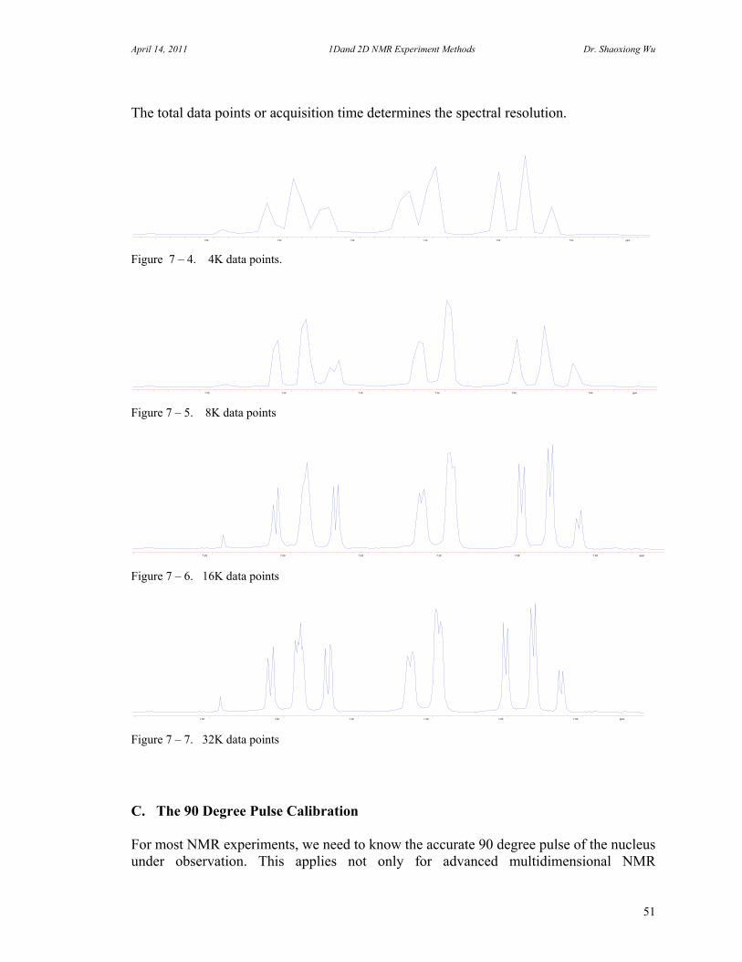
The total data points or acquisition time determines the spectral resolution.
Figure 7 – 4. 4K data points.
Figure 7 – 5. 8K data points
Figure 7 – 6. 16K data points
Figure 7 – 7. 32K data points C. The 90 Degree Pulse Calibration For most NMR experiments, we need to know the accurate 90 degree pulse of the nucleus under observation. This applies not only for advanced multidimensional NMR
7.25 7.20 7.15 7.10 7.05 7.00 ppm
7.25 7.20 7.15 7.10 7.05 7.00 ppm
7.25 7.20 7.15 7.10 7.05 7.00 ppm
7.25 7.20 7.15 7.10 7.05 7.00 ppm

April 14, 2011 1Dand 2D NMR Experiment Methods Dr. Shaoxiong Wu
52
experiments but also for most routine experiments such as INEPT and DEPT. An incorrect pulse width may have a completely different spectrum. The flip angel depends on the RF magnetic field strength B1 (in terms of transmitter power), the pulse width pw (in micro seconds) and the gyromagnetic ratio of the nucleus under observation.
F l i p A n g e l B p w 3 6 0
2 1 (7 – 5)
Usually a 90 degree pulse-length is determined by measuring the length of 180 degree pulse because it gives a null signal (Figure 7-1).
Figure 7-8. Spectra are acquired by INOVA400, the pulse width is increased in 2s for each spectrum. The pulse width of the null signal is 17s at the fixed transmitter power 60. The 90 degree pulse is 8.5 s at tpwr = 60 for proton.
If using different probe, different solvent and different transmitter power, the 90-degree pulse will be different. It should be re-calibrated. For most of 1D experiment, the pulse width is normally set to 72 degree, instead of 90 degree pulse for fast re-pulse. For carbon 1D experiment, one could set the pulse width to 30 degree since the T1 of carbon is very long. If pulse width is set to 90 degree, the pulse delay should be at least 5T1. Decoupler Power Calibration Two homonuclear or heteronuclear spins between which a scalar coupling exists can be effectively decoupled by a variety of methods. In general, NMR instrument has two or three channels, one is tuned to observe nuclear frequency, and the others are tuned to decoupling nuclear frequencies. The transmitter of the observing channel is capable of delivering hard pulses, i.e. high power with a short time. The transmitter of the

April 14, 2011 1Dand 2D NMR Experiment Methods Dr. Shaoxiong Wu
53
decoupling channel is capable of delivering soft pulses, i.e. low power with a longer time. There are several parameters to control the decoupling channel; decoupling power, decoupling frequency, 90-degree pulse width, decoupling mode. For proton decoupling while observing other nuclei such as 13C and 31P, the decoupling power can be calibrated by determining the H2 at a given decoupler power level. Using a standard sample, doped 40% Dioxane in benzene-D6, tune the probe for 13C (observe channel) and 1H (decoupling channel). If the probe is used to detect other nuclei, rather than 13C, it is necessary to check the tuning twice since when tune the f1 channel the f2 channel frequency may be slightly changed. 1. Take a proton spectrum, and set the decoupler frequency at the CH2 peak.
Figure 7 – 9. Proton spectrum of dioxane in benzene_D6. 2. Take a carbon spectrum with decoupler power off. Measure the coupling constant of CH2 (It should be 142Hz and it is independent of instrument field).
10 8 6 4 2 0 ppm
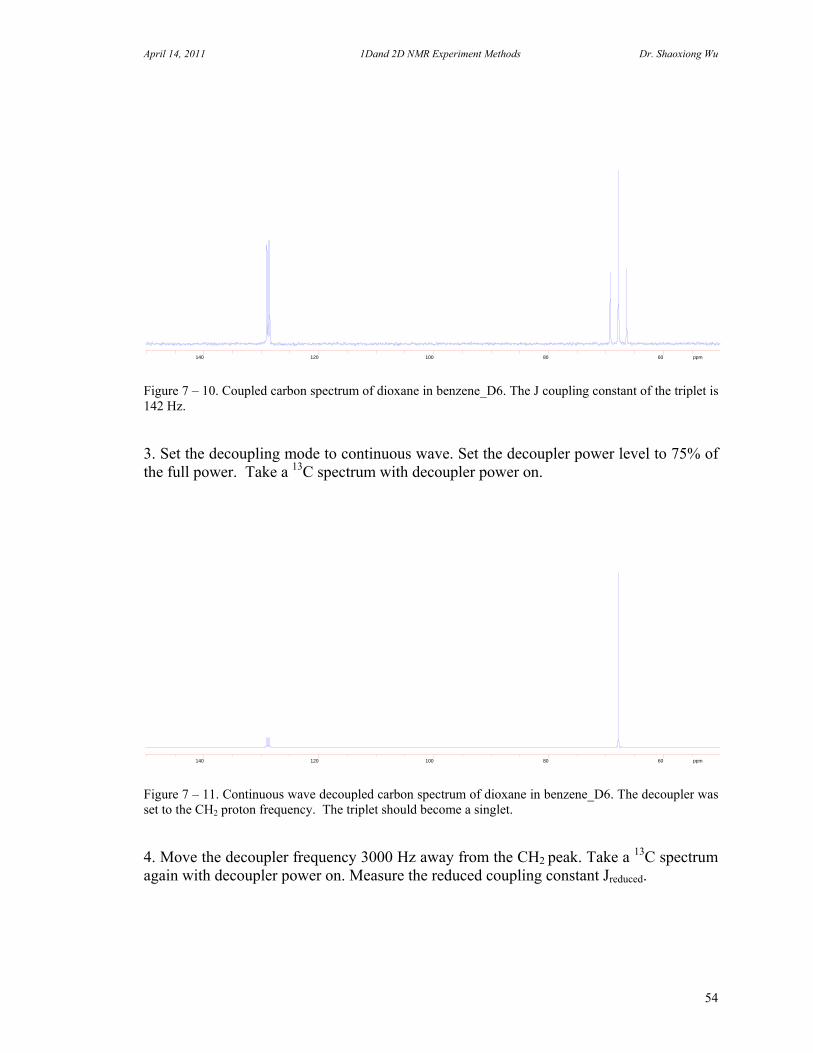
April 14, 2011 1Dand 2D NMR Experiment Methods Dr. Shaoxiong Wu
54
Figure 7 – 10. Coupled carbon spectrum of dioxane in benzene_D6. The J coupling constant of the triplet is 142 Hz. 3. Set the decoupling mode to continuous wave. Set the decoupler power level to 75% of the full power. Take a 13C spectrum with decoupler power on.
Figure 7 – 11. Continuous wave decoupled carbon spectrum of dioxane in benzene_D6. The decoupler was set to the CH2 proton frequency. The triplet should become a singlet. 4. Move the decoupler frequency 3000 Hz away from the CH2 peak. Take a 13C spectrum again with decoupler power on. Measure the reduced coupling constant Jreduced.
140 120 100 80 60 ppm
140 120 100 80 60 ppm
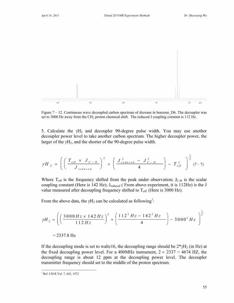
April 14, 2011 1Dand 2D NMR Experiment Methods Dr. Shaoxiong Wu
55
Figure 7 – 12. Continuous wave decoupled carbon spectrum of dioxane in benzene_D6. The decoupler was set to 3000 Hz away from the CH2 proton chemical shift. The reduced J coupling constant is 112 Hz.
5. Calculate the H2 and decoupler 90-degree pulse width. You may use another decoupler power level to take another carbon spectrum. The higher decoupler power, the larger of the H2, and the shorter of the 90-degree pulse width.
HT J
J
J JTo f f C H
r e d u c e d
r e d u c e d C Ho f f2
2 2 22
1
2
4
(7 – 7)
Where Toff is the frequency shifted from the peak under observation; JC-H is the scalar coupling constant (Here is 142 Hz); Jreduced ( From above experiment, it is 112Hz) is the J value measured after decoupling frequency shifted to Toff (Here is 3000 Hz). From the above data, the H2 can be calculated as following1:
HH z H z
H z
H z H zH z2
2 2 2
2
1
23 0 0 0 1 4 2
1 1 2
1 1 2 1 4 2
43 0 0 0
= 2337.8 Hz If the decoupling mode is set to waltz16, the decoupling range should be 2*H2 (in Hz) at the fixed decoupling power level. For a 400MHz instrument, 2 2337 = 4674 HZ, the decoupling range is about 12 ppm at the decoupling power level. The decoupler transmitter frequency should set to the middle of the proton spectrum.
1 Ref. J.M.R Vol. 7, 442, 1972
140 120 100 80 60 ppm
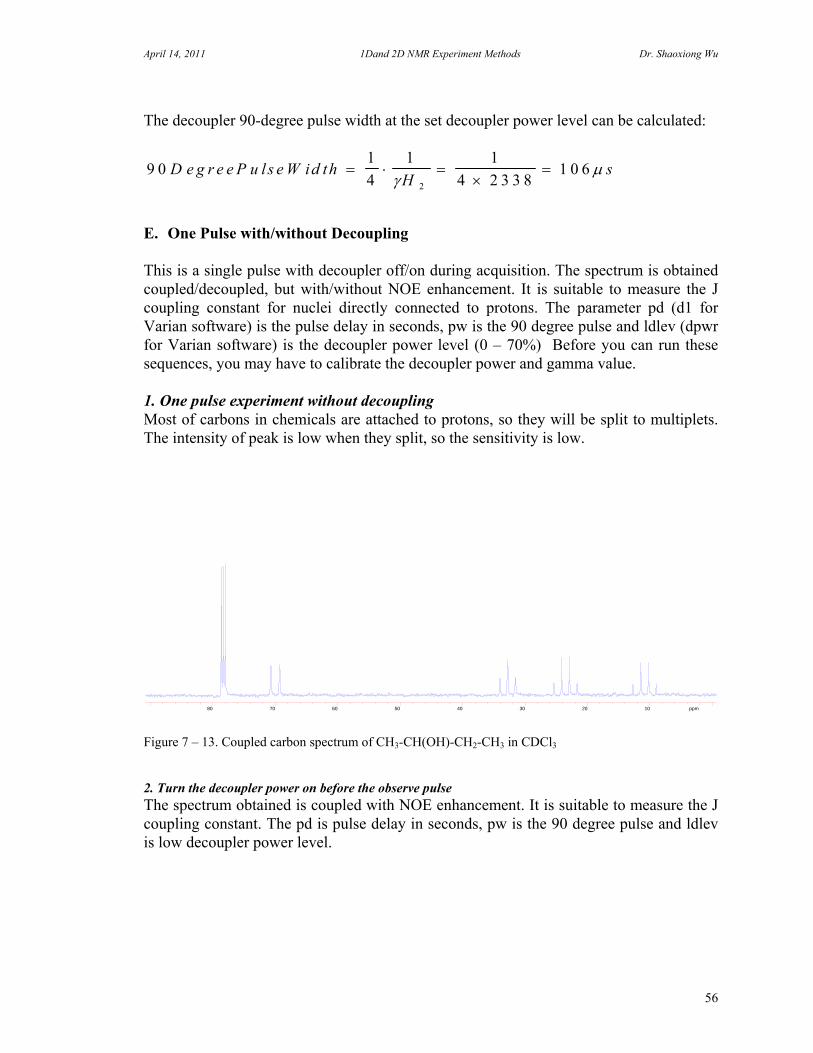
April 14, 2011 1Dand 2D NMR Experiment Methods Dr. Shaoxiong Wu
56
The decoupler 90-degree pulse width at the set decoupler power level can be calculated:
9 01
4
1 1
4 2 3 3 81 0 6
2
D e g r e e P u ls e W id thH
s
E. One Pulse with/without Decoupling This is a single pulse with decoupler off/on during acquisition. The spectrum is obtained coupled/decoupled, but with/without NOE enhancement. It is suitable to measure the J coupling constant for nuclei directly connected to protons. The parameter pd (d1 for Varian software) is the pulse delay in seconds, pw is the 90 degree pulse and ldlev (dpwr for Varian software) is the decoupler power level (0 – 70%) Before you can run these sequences, you may have to calibrate the decoupler power and gamma value. 1. One pulse experiment without decoupling Most of carbons in chemicals are attached to protons, so they will be split to multiplets. The intensity of peak is low when they split, so the sensitivity is low.
Figure 7 – 13. Coupled carbon spectrum of CH3-CH(OH)-CH2-CH3 in CDCl3 2. Turn the decoupler power on before the observe pulse The spectrum obtained is coupled with NOE enhancement. It is suitable to measure the J coupling constant. The pd is pulse delay in seconds, pw is the 90 degree pulse and ldlev is low decoupler power level.
80 70 60 50 40 30 20 10 ppm

April 14, 2011 1Dand 2D NMR Experiment Methods Dr. Shaoxiong Wu
57
Figure 7 – 14. One Pulse sequence with decoupler is turned on before the observe pulse.
Figure 7 –15. Coupled carbon spectrum of CH3-CH(OH)-CH2-CH3 in CDCl3 with NOE enhancement. 3. Turn the decoupler power on after the observe pulse The spectrum obtained is decoupled without NOE. It is suitable to some nuclei with negative megnetogyric ratio.
Figure 7 – 16. One pulse sequence with decoupler is turned on after observe pulse.
pd
pw
Acquisition
X
ldlev
80 70 60 50 40 30 20 10 ppm
pd
pw
Acquisition
X
ldlev
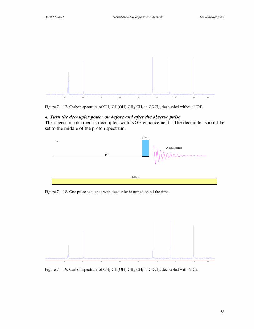
April 14, 2011 1Dand 2D NMR Experiment Methods Dr. Shaoxiong Wu
58
Figure 7 – 17. Carbon spectrum of CH3-CH(OH)-CH2-CH3 in CDCl3, decoupled without NOE. 4. Turn the decoupler power on before and after the observe pulse The spectrum obtained is decoupled with NOE enhancement. The decoupler should be set to the middle of the proton spectrum.
Figure 7 – 18. One pulse sequence with decoupler is turned on all the time.
Figure 7 – 19. Carbon spectrum of CH3-CH(OH)-CH2-CH3 in CDCl3, decoupled with NOE.
80 70 60 50 40 30 20 10 ppm
pd
pw
Acquisition
X
ldlev
80 70 60 50 40 30 20 10 ppm

April 14, 2011 1Dand 2D NMR Experiment Methods Dr. Shaoxiong Wu
59
Figure 7 – 20. Part of carbon spectra of CH3-CH(OH)-CH3 in Acetone_D6. They are acquired with same number of scans and same experiment parameters. From the top: H decoupler off; H decoupler turned on before pulse; H decoupler turned on after pulse and H decoupler turned on all the time. This pulse sequence also can be used as off-resonance decoupling. In a broadband proton decoupling spectrum, the multiplicity of each signal cannot be determined since all of carbon signal of CH3, CH2, CH and C will be a singlet. The off-resonance decoupling allows us to observe the multiplicity and simplify the coupled spectrum. The spin spin coupling constant in off-resonance proton decoupling spectrum is reduced to several tens of Hz. There is thus relatively little signal overlap.
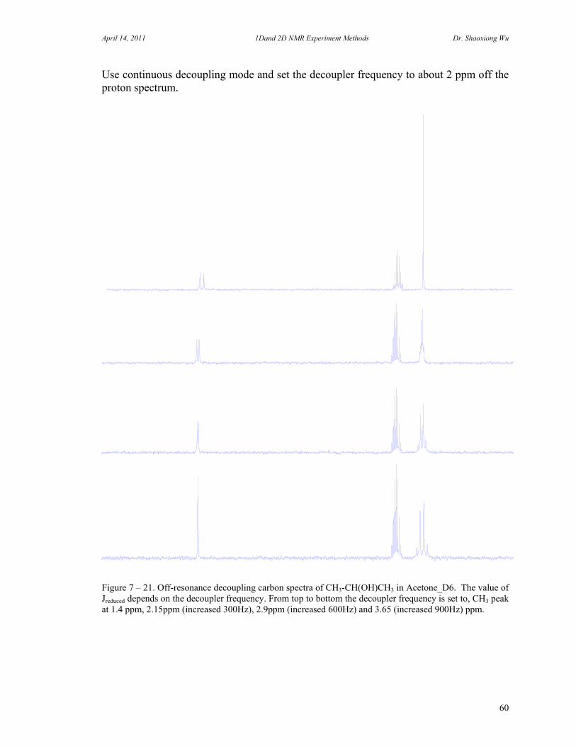
April 14, 2011 1Dand 2D NMR Experiment Methods Dr. Shaoxiong Wu
60
Use continuous decoupling mode and set the decoupler frequency to about 2 ppm off the proton spectrum. Figure 7 – 21. Off-resonance decoupling carbon spectra of CH3-CH(OH)CH3 in Acetone_D6. The value of Jreduced depends on the decoupler frequency. From top to bottom the decoupler frequency is set to, CH3 peak at 1.4 ppm, 2.15ppm (increased 300Hz), 2.9ppm (increased 600Hz) and 3.65 (increased 900Hz) ppm.

April 14, 2011 1Dand 2D NMR Experiment Methods Dr. Shaoxiong Wu
61
5. Homonuclear decoupling Homonuclear decoupling on FT NMR instruments with a single proton tunable coil probe requires a special decoupler mode, since the preamplifier must be protected against the decoupler RF power. This can be done by applying the decoupling pulse only between the digitization point or during the dwell time with the preamplifier blanked. For single resonance homonuclear decoupling, the presaturation pulse sequence may be used:
Figure 7 – 22. Presaturation pulse sequence. The decoupler is set to continuous wave mode. The dlevel is the decoupling power.
Figure 7 – 23. A part of proton spectrum of strychnine in CDCl3.
Figure 7 – 24. Homodecoupling spectrum of strychnine in CDCl3. The decoupler is set to 1.8ppm at the peak 17. The peaks at 2.8 and 3.2ppm are decoupled, i.e. two protons at position 18 in the following structure.
dlevel
pw
Acquisitionpre-saturation delaypd
4.5 4.0 3.5 3.0 2.5 2.0 1.5 ppm
4.5 4.0 3.5 3.0 2.5 2.0 1.5 ppm
18
18
17
1818
17
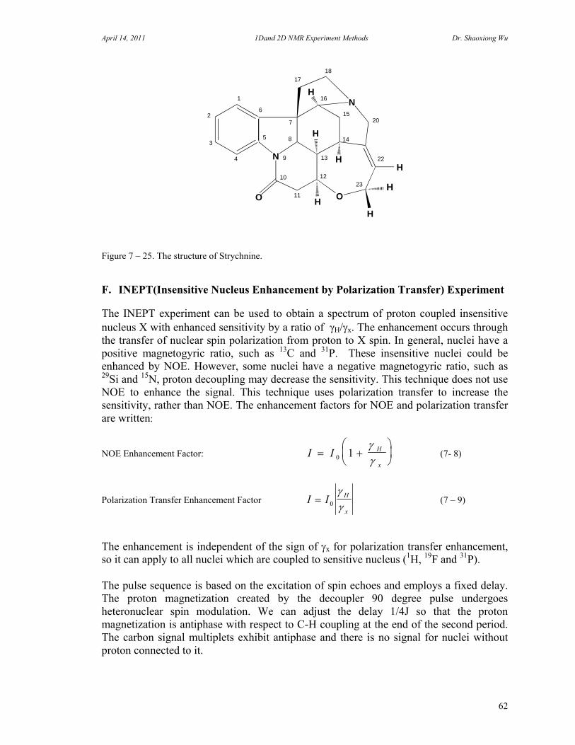
April 14, 2011 1Dand 2D NMR Experiment Methods Dr. Shaoxiong Wu
62
Figure 7 – 25. The structure of Strychnine. F. INEPT(Insensitive Nucleus Enhancement by Polarization Transfer) Experiment The INEPT experiment can be used to obtain a spectrum of proton coupled insensitive nucleus X with enhanced sensitivity by a ratio of H/x. The enhancement occurs through the transfer of nuclear spin polarization from proton to X spin. In general, nuclei have a positive magnetogyric ratio, such as 13C and 31P. These insensitive nuclei could be enhanced by NOE. However, some nuclei have a negative magnetogyric ratio, such as 29Si and 15N, proton decoupling may decrease the sensitivity. This technique does not use NOE to enhance the signal. This technique uses polarization transfer to increase the sensitivity, rather than NOE. The enhancement factors for NOE and polarization transfer are written:
NOE Enhancement Factor: I I H
x
0 1
(7- 8)
Polarization Transfer Enhancement Factor I I H
x
0
(7 – 9)
The enhancement is independent of the sign of x for polarization transfer enhancement, so it can apply to all nuclei which are coupled to sensitive nucleus (1H, 19F and 31P). The pulse sequence is based on the excitation of spin echoes and employs a fixed delay. The proton magnetization created by the decoupler 90 degree pulse undergoes heteronuclear spin modulation. We can adjust the delay 1/4J so that the proton magnetization is antiphase with respect to C-H coupling at the end of the second period. The carbon signal multiplets exhibit antiphase and there is no signal for nuclei without proton connected to it.
N
O
N1
2
3
4
8
7
17
H16
5
6
9 13
HH
H
H
H
OH
18
20
22
23
11
10
15
14
12

April 14, 2011 1Dand 2D NMR Experiment Methods Dr. Shaoxiong Wu
63
Figure 7 – 26. INEPT pulse sequence.
Figure 7 – 27. Decoupled INEPT spectrum of CH3-CH(OH)-CH2-CH3 in CDCl3. Two CH3 and CH are up and CH2 is down. The carbons without protons are eliminated. In some cases, this is a very useful method to eliminate big solvent peak. In this case, the CDCl3 peak is eliminated completely.
Figure 7 – 28. Coupled INEPT spectrum of CH3-CH(OH)-CH2-CH3 in CDCl3. From the spectrum, the important structure information, J coupling constants still can be measured.
pd
p90
Acquisition
p180
d90d90 d180
1/4J
1/4J1/4J
X-Nucleus
H-decoupler
Decoupling
80 60 40 20 ppm
80 60 40 20 ppm
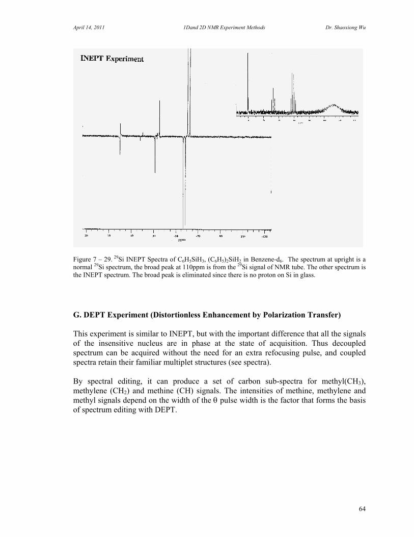
April 14, 2011 1Dand 2D NMR Experiment Methods Dr. Shaoxiong Wu
64
Figure 7 – 29. 29Si INEPT Spectra of C6H5SiH3, (C6H5)2SiH2 in Benzene-d6. The spectrum at upright is a normal 29Si spectrum, the broad peak at 110ppm is from the 29Si signal of NMR tube. The other spectrum is the INEPT spectrum. The broad peak is eliminated since there is no proton on Si in glass. G. DEPT Experiment (Distortionless Enhancement by Polarization Transfer) This experiment is similar to INEPT, but with the important difference that all the signals of the insensitive nucleus are in phase at the state of acquisition. Thus decoupled spectrum can be acquired without the need for an extra refocusing pulse, and coupled spectra retain their familiar multiplet structures (see spectra).
By spectral editing, it can produce a set of carbon sub-spectra for methyl(CH3), methylene (CH2) and methine (CH) signals. The intensities of methine, methylene and methyl signals depend on the width of the pulse width is the factor that forms the basis of spectrum editing with DEPT.

April 14, 2011 1Dand 2D NMR Experiment Methods Dr. Shaoxiong Wu
65
Figure 7 – 30. DEPT pulse sequence.
The J value is the average value of JC-H coupling constants. The can be set to 45, 90 and 135 degree pulse. If = 45, all protonated carbon give a positive peaks. If =90, only CH carbon can be observed, both CH2 and CH3 will be null signals. If = 135, the CH and CH3 signals will be positive and CH2 signals will be negative.
Figure 7 – 31. Plot of intensities of methine, methylene and methyl signals versus pulse width of .
pd
d90 d180H-decoupler
Decoupling
1/2J1/2J1/2J
p90
Acquisition
p180
1/2J
X-Nucleus
1/2J
CH 3
CH 2
CH
0 45 90 135 180

April 14, 2011 1Dand 2D NMR Experiment Methods Dr. Shaoxiong Wu
66
Figure 7 – 32. DEPT spectrum of CH3-CH(OH)-CH2-CH3 in CDCl3. The is set to 45 degree.
Figure 7 – 33. DEPT spectrum of CH3-CH(OH)-CH2-CH3 in CDCl3. The is set to 90 degree.
Figure 7 – 34. DEPT spectrum of CH3-CH(OH)-CH2-CH3 in CDCl3. The is set to 135 degree. After edit above spectra, you could obtain edited spectrum that prints out CH, CH2 and CH3 separately. It is very useful for signing a 13C spectrum.
80 60 40 20 ppm
80 60 40 20 ppm
80 60 40 20 ppm
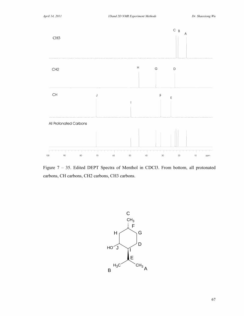
April 14, 2011 1Dand 2D NMR Experiment Methods Dr. Shaoxiong Wu
67
Figure 7 – 35. Edited DEPT Spectra of Menthol in CDCl3. From bottom, all protonated
carbons, CH carbons, CH2 carbons, CH3 carbons.
CH3
CH3 CH3
OH
AB
C
D
GH
J I
E
F

April 14, 2011 1Dand 2D NMR Experiment Methods Dr. Shaoxiong Wu
68
H. Water Suppression Experiments In biological NMR spectroscopy, there are many instances where it may be desirable to record both one- and two-dimensional spectra in the presence of a high concentration of solvent water (typically 90% H2O with 10% D2O). It is necessary to suppress the strong water resonance so that the dynamic range of the receiver or the ADC does not overflow. There are several techniques by which the strong water resonance or other solvent resonance can be suppressed. The simplest one is presaturation, i.e. apply a weak RF field at the solvent frequency. However, this technique is not ideal since the protons that are in chemical exchange with the solvent such as NH's and OH's may also be partially saturated due to saturation transfer. The second technique is Inversion recovery, i.e. the sequence is adjusted such that solvent resonance lies at the null point whereas the signals derived from the molecule have fully relaxed. 1. The Jump-and-Return Sequence
This sequence consists of two 90 pulses of opposite phase separated by an adjustable delay. The effective flip angle is zero for the transmitter frequency (solvent frequency is set to transmitter frequency) i.e. the magnetization is flipped into xy plane in the rotating frame, experiences no precession during the delay. This magnetization will be returned to the +Z axis by the second 90 pulse so that it contributes no signal. However, other magnetization will precess during the delay and are not returned fully along the +Z axis by the second 90 pulse. Since the precession is proportional to the offset, the flip angle is variable off resonance, and is adjusted by both the offset and the pulse delay. The spectrum will be a 180 phase difference about the on resonance condition.
Figure 7 – 36. 11 jump return water suppression pulse sequence. Where pwa is the 90 degree pulse, pwb =
pwa - 0.l s and dl inter pulse delay calculated from the spectrum width deltav. d1=1/2deltav.
pwb
Acquisition
pd
pwa
d1
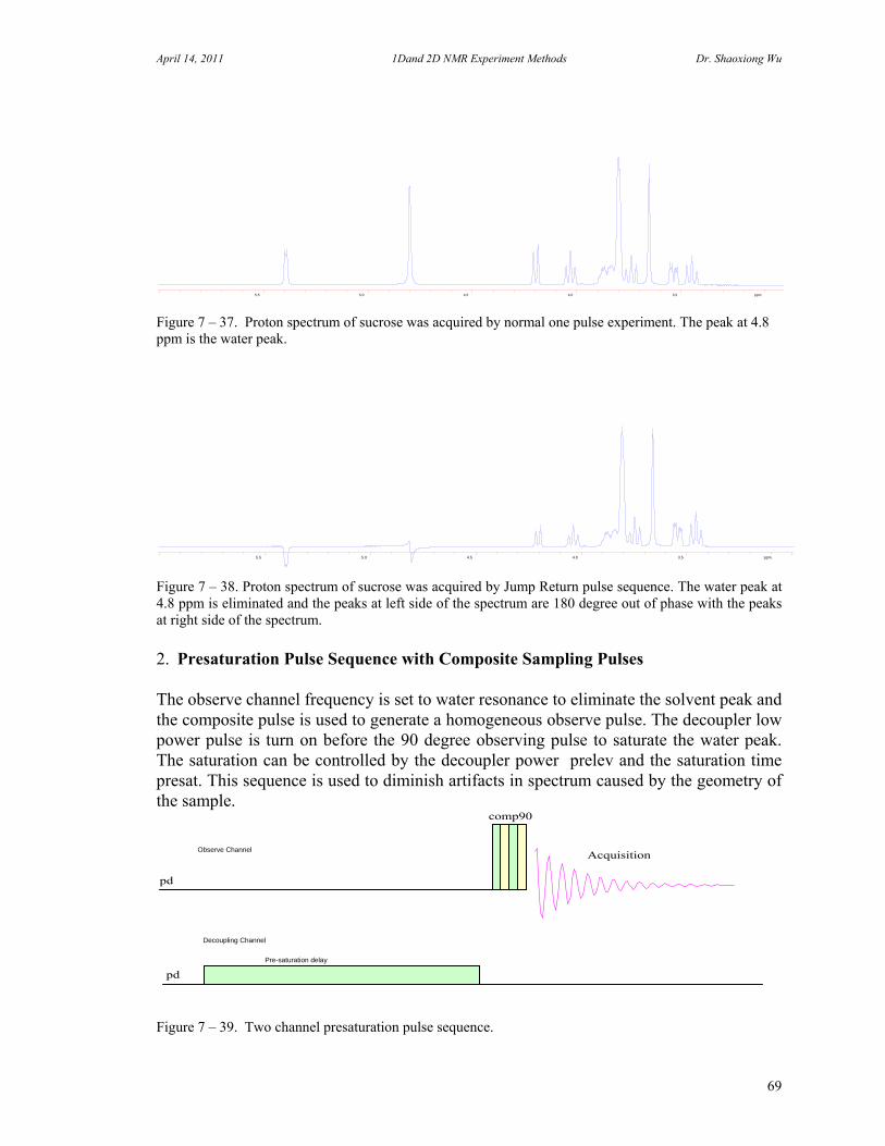
April 14, 2011 1Dand 2D NMR Experiment Methods Dr. Shaoxiong Wu
69
Figure 7 – 37. Proton spectrum of sucrose was acquired by normal one pulse experiment. The peak at 4.8 ppm is the water peak.
Figure 7 – 38. Proton spectrum of sucrose was acquired by Jump Return pulse sequence. The water peak at 4.8 ppm is eliminated and the peaks at left side of the spectrum are 180 degree out of phase with the peaks at right side of the spectrum. 2. Presaturation Pulse Sequence with Composite Sampling Pulses The observe channel frequency is set to water resonance to eliminate the solvent peak and the composite pulse is used to generate a homogeneous observe pulse. The decoupler low power pulse is turn on before the 90 degree observing pulse to saturate the water peak. The saturation can be controlled by the decoupler power prelev and the saturation time presat. This sequence is used to diminish artifacts in spectrum caused by the geometry of the sample.
Figure 7 – 39. Two channel presaturation pulse sequence.
5.5 5.0 4.5 4.0 3.5 ppm
5.5 5.0 4.5 4.0 3.5 ppm
comp90
Acquisition
pd
Pre-saturation delay
Observe Channel
Decoupling Channel
pd
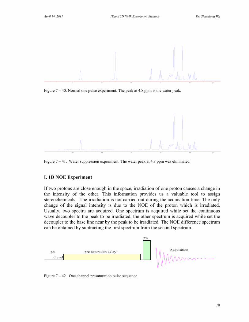
April 14, 2011 1Dand 2D NMR Experiment Methods Dr. Shaoxiong Wu
70
Figure 7 – 40. Normal one pulse experiment. The peak at 4.8 ppm is the water peak.
Figure 7 – 41. Water suppression experiment. The water peak at 4.8 ppm was eliminated. I. 1D NOE Experiment If two protons are close enough in the space, irradiation of one proton causes a change in the intensity of the other. This information provides us a valuable tool to assign stereochemicals. The irradiation is not carried out during the acquisition time. The only change of the signal intensity is due to the NOE of the proton which is irradiated. Usually, two spectra are acquired. One spectrum is acquired while set the continuous wave decoupler to the peak to be irradiated; the other spectrum is acquired while set the decoupler to the base line near by the peak to be irradiated. The NOE difference spectrum can be obtained by subtracting the first spectrum from the second spectrum.
Figure 7 – 42. One channel presaturation pulse sequence.
5.5 5.0 4.5 4.0 3.5 ppm
5.5 5.0 4.5 4.0 3.5 ppm
dlevel
pw
Acquisitionpre-saturation delaypd
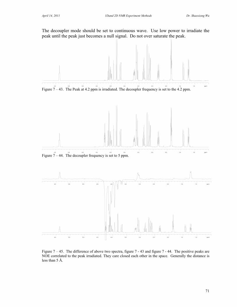
April 14, 2011 1Dand 2D NMR Experiment Methods Dr. Shaoxiong Wu
71
The decoupler mode should be set to continuous wave. Use low power to irradiate the peak until the peak just becomes a null signal. Do not over saturate the peak.
Figure 7 – 43. The Peak at 4.2 ppm is irradiated. The decoupler frequency is set to the 4.2 ppm.
Figure 7 – 44. The decoupler frequency is set to 5 ppm.
Figure 7 – 45. The difference of above two spectra, figure 7 - 43 and figure 7 - 44. The positive peaks are NOE correlated to the peak irradiated. They care closed each other in the space. Generally the distance is less than 5 Å.
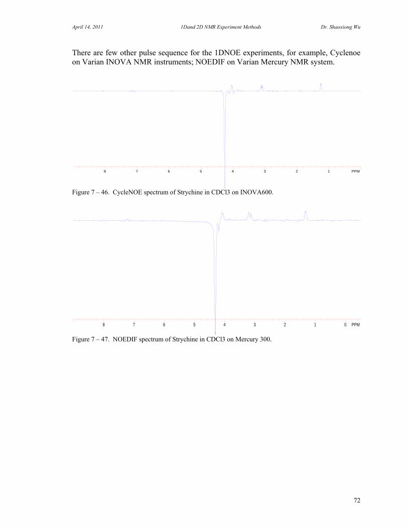
April 14, 2011 1Dand 2D NMR Experiment Methods Dr. Shaoxiong Wu
72
There are few other pulse sequence for the 1DNOE experiments, for example, Cyclenoe on Varian INOVA NMR instruments; NOEDIF on Varian Mercury NMR system.
Figure 7 – 46. CycleNOE spectrum of Strychine in CDCl3 on INOVA600.
Figure 7 – 47. NOEDIF spectrum of Strychine in CDCl3 on Mercury 300.
8 7 6 5 4 3 2 1 PPM
8 7 6 5 4 3 2 1 0 PPM

April 14, 2011 1Dand 2D NMR Experiment Methods Dr. Shaoxiong Wu
73
J. 13C Spectrum with Fluorine Decoupling
In general, 19F spectrum has large spectrum width, about 100 ppm (56400 Hz for a 600 MHz instrument). When we acquire a 13C spectrum with these fluorated compounds, it is very difficulty to decouple all 19F peaks in the range.
Figure 7- 46. 19F spectrum of (CF3)2CCFCF2CF3 in Acetone_D6 acquired on INOVA600.
Figure 7-47. 13C spectrum of (CF3)2CCFCF2CF3 in Acetone_D6 was acquired on INOVA600 without 19F decoupling.
70 60 50 40 30 20 10 0 PPM
250 200 150 100 50 0 PPM
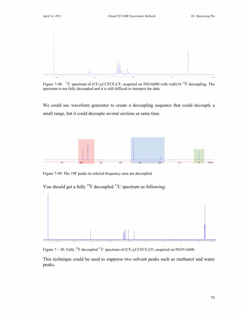
April 14, 2011 1Dand 2D NMR Experiment Methods Dr. Shaoxiong Wu
74
Figure 7-48. 13C spectrum of (CF3)2CCFCF2CF3 acquired on INOA600 with waltz16 19F decoupling. The spectrum is not fully decoupled and it is still difficult to interpret the data.
We could use waveform generator to create a decoupling sequence that could decouple a
small range, but it could decouple several sections at same time.
Figure 7-49. The 19F peaks in colored frequency area are decoupled. You should get a fully 19F decoupled 13C spectrum as following:
Figure 7 – 50. Fully 19F decoupled 13C spectrum of (CF3)2CCFCF2CF3 acquired on INOVA600. This technique could be used to suppress two solvent peaks such as methanol and water peaks.
200 150 100 50 PPM
70 60 50 40 30 20 10 0 PPM
2 0 0 1 8 0 1 6 0 1 4 0 1 2 0 1 0 0 8 0 6 0 4 0 P P M
April 14, 2011 1Dand 2D NMR Experiment Methods Dr. Shaoxiong Wu
75
K. Molecular Self-diffusion Studies by NMR The diffusion process both in solution and solid state NMR has been studied for many years by a variety of methods. The reason is that self-diffusion data provides uniquely detailed and easily interpreted information on molecular organization, phase structure and the relative properties of sorbent and sorbate. On the other hand, self-diffusion coefficients are quite sensitive to structural change; in particular, for colloidal or macromolecular systems in solution the experimental self-diffusion coefficient is directly related to molecular displacement in the laboratory coordinates which provides information about restricted molecular motion in some systems. For example, to study ligand-protein binding, diffusion coefficients can discriminate between large and small molecules. For homogeneous and heterogeneous catalytic reaction studies, the mobility of molecules may provide key information about reaction mechanisms and dynamic equilibrium. Self-diffusion measurements by PFG NMR have been applied in numerous fields ever since the first diffusion measurement experiment. The technique usually requires no special labeling, which is a significant advantage when compared with using radioisotopes or photo-labeled molecules because no special sample preparation or handling is required. A single set of measurements can yield diffusion coefficients and often can be done in less than a few hours. When compared with the adsorption rate measurement method, it is faster and more accurate. For high field FT-NMR with a pulsed field gradient unit, another unique advantage is that it makes it possible to measure diffusion coefficients of protons at different positions in the same molecule. This is very useful for the study physical and chemical properties of polymers. Since the discovery of the spin echo pulse sequence, several effects on spin echo were discovered and correctly interpreted by Stejskal et al. One of which was the diffusion effect on echo amplitudes in an inhomogeneous magnetic field. This important effect was evidently put forward by McCall et al. and one year later Stejskal, Tanner presented the first successful diffusion measurement experiment. Since then, the technique has been heavily utilized for investigations of molecular transportation behavior. The applications of PFG NMR diffusion data for probing liquid state molecular organization, investigating molecular self-diffusion in solids and studying molecule restrict self-diffusion in cells have been reported. Meerwall has been using PFG NMR to investigate molecular transport in polymeric systems. The utilization of PFG NMR techniques for studies of ionic diffusion in solid electrolytes has been done by Whittengham. The technique has become a powerful tool to monitor molecular mobility in a variety of materials. The most satisfactory method for measuring self-diffusion coefficients is the spin-echo by Hahn, as developed by Carr, Purcell and others. The basic spin-echo pulse sequence consists of two RF pulses, a 90 degree pulse followed by a second pulse, 180 degree after a time interval τ. The 90-τ-180-τ-echo pulse sequence can be described in terms of the classical vector picture. (Figure 7 - 51) The first pulse rotates the nuclear magnetization vector M away from its equilibrium orientation along the laboratory magnetic field Bo onto the X-Y plane. Following this pulse, we can detect a nuclear signal by observing Mx or My on the rotating frame. During the first time interval τ, spins with different frequencies, due to chemical shift and other interactions, continue to precess about Bo and dephase on the X-

April 14, 2011 1Dand 2D NMR Experiment Methods Dr. Shaoxiong Wu
76
Y plane. The time required to lose phase coherence, T2, is determined partly by the uniformity of the field over the volume of the sample, since the precession frequency of a particular spin is proportional to the strength of the magnetic field at the site. The effect of the second pulse is to reverse the precessing directions of the spins and to invert the phase errors which have built up since the first pulse. Those spins which had accumulated positive or negative phase errors are rotated by the 180 pulse until they find themselves with equivalent positive or negative errors. Phase coherence is regained as fast as it is lost and at 2τ, the recovery of phase coherence is complete and a spin echo occurs. The spins may experience random phase shifts which cause loss of phase memory. So, the intensity of the echo depends on T2. Molecular self-diffusion will also result in a reduced echo, because the loss of phase coherence was partly due to the field uniformity. If a spin moves during the time τ so as to experience the varying field, its frequency will also vary and the spin may not regain phase coherence along with the other spins. Consequently they will not contribute to the spin echo intensity. This principle leads the molecular self-diffusion measurement. In order to study molecular diffusion, a linear magnetic gradient field is imposed on the sample.
X
Y
Z
X
Y
Z
X
Y '
Z' = Z
'
( A ) ( B )
( C ) ( D )
X '
Y '
Z
90 Degree Pulse
180 Pulse along the Y axis
After
Delay
Aft
er
De
lay
Figure 7 – 51. Classical vector picture of spin echo. Spins could be refocused at 2 τ. If we insert two identical gradient field pulses between 90 degree pulse and 180 degree pulse, 180 degree pulse and echo (Figure 7 - 52) the spins still can be refocused, but its amplitude is directly affected by the molecule self-diffusion. This occurs because under the gradient field, the frequency of a particular spin changes when it moves. Because of the random motion of the molecules in the gradient field, spins are unable to refuse perfectly at 2τ.
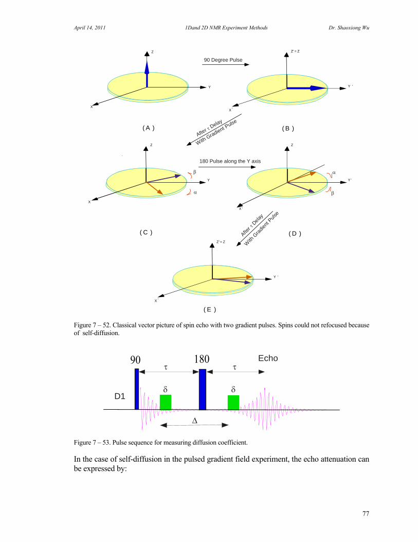
April 14, 2011 1Dand 2D NMR Experiment Methods Dr. Shaoxiong Wu
77
X
Y '
Z' = Z
'X
Y
Z
X
Y
Z
( A ) ( B )
( C ) ( D )
X '
Y '
Z
90 Degree Pulse
180 Pulse along the Y axis
After
Delay
WithGradient Pulse
X
Y '
Z' = Z
'
After
Delay
With
Gradie
ntPul
se
( E ) Figure 7 – 52. Classical vector picture of spin echo with two gradient pulses. Spins could not refocused because of self-diffusion.
18090 Echo
D1
Figure 7 – 53. Pulse sequence for measuring diffusion coefficient. In the case of self-diffusion in the pulsed gradient field experiment, the echo attenuation can be expressed by:

April 14, 2011 1Dand 2D NMR Experiment Methods Dr. Shaoxiong Wu
78
where:
G = Pulse field gradient (Gause/cm.A).
δ = Length of time the field gradient pulse is applied (ms).
Δ = Time between start of first field gradient pulse and the start of
the second field gradient pulse (ms).
A0 = Echo attenuation without field gradient.
A = Echo attenuation with field gradient.
The experiments are typically performed with Δ fixed and δ regularly incremented while keeping G constant. If we plot the time, δ, against the echo attenuation A, then from the slope the effective diffusion coefficient can be calculated by comparing to samples with known diffusion constants. There are some important experimental aspects such as gradient pulse calibrations, sample temperature dependent, sample volume etc. This technique has been widely used in different applications, it will continuous to be developed. Diffusion Ordered spectroscopy (DOSY) The principles of the DOSY experiment is applying two gradient pulses between 90 and 180 degree pulse (spin echo), then measure the intensity of the echo. Plot the intensity of the echo vs the strength of the gradient pulse, we can calculate the diffusion coefficient of the molecule. A DOSY spectrum, x-axis is the chemical shifts same as the regular 1D spectrum, y-axis is the diffusion coefficients. If the sample is a mixture, the two compounds in the solution have two different diffusion rate, then the DOSY will show two separated line in the y-axis, each of them is relative to one compound with their chemical shifts on the x-axis.
)3
()2(
)2( 222
0
GD
A
ALn
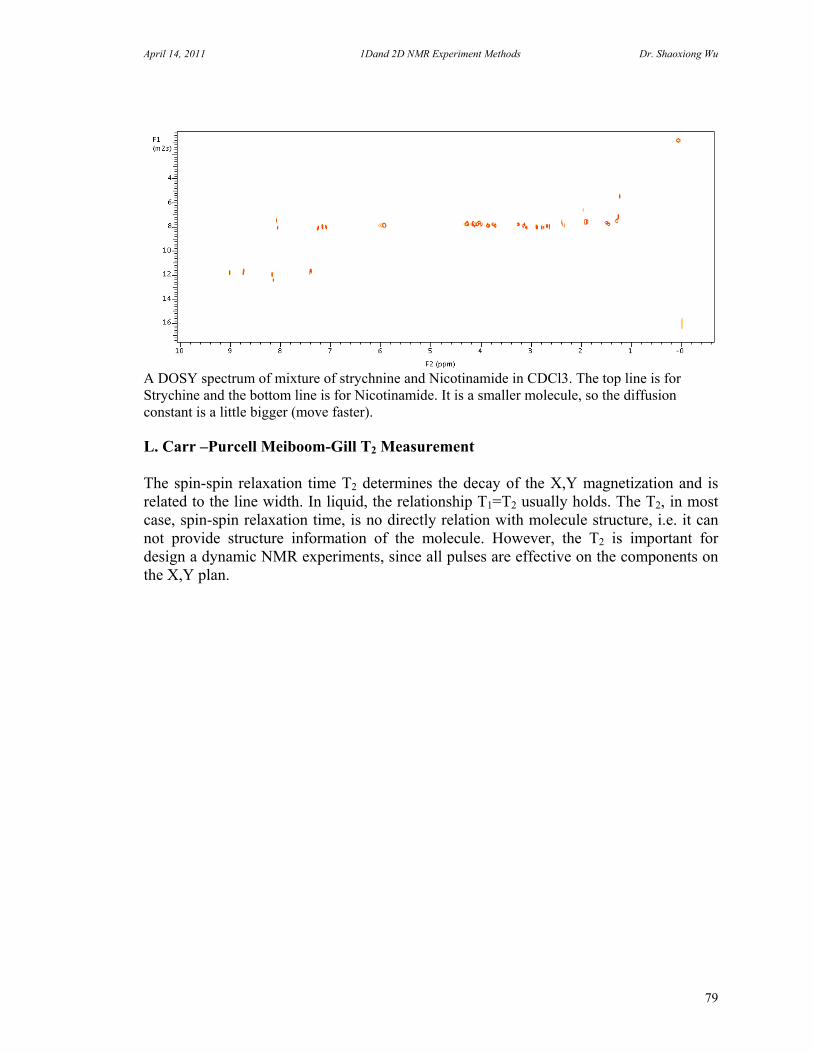
April 14, 2011 1Dand 2D NMR Experiment Methods Dr. Shaoxiong Wu
79
A DOSY spectrum of mixture of strychnine and Nicotinamide in CDCl3. The top line is for Strychine and the bottom line is for Nicotinamide. It is a smaller molecule, so the diffusion constant is a little bigger (move faster). L. Carr –Purcell Meiboom-Gill T2 Measurement The spin-spin relaxation time T2 determines the decay of the X,Y magnetization and is related to the line width. In liquid, the relationship T1=T2 usually holds. The T2, in most case, spin-spin relaxation time, is no directly relation with molecule structure, i.e. it can not provide structure information of the molecule. However, the T2 is important for design a dynamic NMR experiments, since all pulses are effective on the components on the X,Y plan.
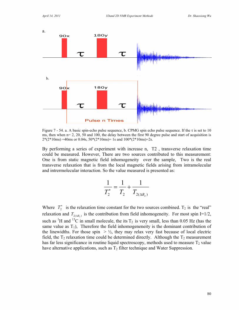
April 14, 2011 1Dand 2D NMR Experiment Methods Dr. Shaoxiong Wu
80
a.
b.
Figure 7 - 54. a. A basic spin-echo pulse sequence, b. CPMG spin echo pulse sequence. If the τ is set to 10 ms, then when n= 2, 20, 50 and 100, the delay between the first 90 degree pulse and start of acquisition is 2*(2*10ms) =40ms or 0.04s, 50*(2*10ms)= 1s and 100*(2*10ms)=2s. By performing a series of experiment with increase n, T2 , transverse relaxation time could be measured. However, There are two sources contributed to this measurement: One is from static magnetic field inhomogeneity over the sample, Two is the real transverse relaxation that is from the local magnetic fields arising from intramolecular and intrermolecular interaction. So the value measured is presented as:
)(222
111
oBTTT
Where
2T is the relaxation time constant for the two sources combined. T2 is the “real” relaxation and )(2 oBT is the contribution from field inhomogeneity. For most spin I=1/2,
such as 1H and 13C in small molecule, the its T2 is very small, less than 0.05 Hz (has the same value as T1), Therefore the field inhomogeneneity is the dominant contribution of the linewidths. For those spin > ½, they may relax very fast because of local electric field, the T2 relaxation time could be determined directly. Although the T2 measurement has far less significance in routine liquid spectroscopy, methods used to measure T2 value have alternative applications, such as T2 filter technique and Water Suppression.
180y90x

April 14, 2011 1Dand 2D NMR Experiment Methods Dr. Shaoxiong Wu
81
Figure 7 - 55, Proton spectra of human plasma samples. Top: 1D proton spectrum with water suppression. The baseline is broadened because of immobile protons of the proteins and albumin-bound fatty acids (They have short T2s). Bottom: Using CPMG spin echo sequence, the baseline is corrected, all low molecular weight metabolites are showed as sharp peaks (they have long T2s). This technique lies in the difference in T2 of different molecular size. Larger molecules have short T2 and broader line width. Smaller molecules have long T2 and sharper line width. If we could edit the pulse sequence that only allows molecules with longer T2 remain in the XY plan, then we could filtered out these resonance from big molecules (broader peaks). This application has been widely used in the study of blood samples.
10 8 6 4 2 0 PPM
10 8 6 4 2 0 PPM

April 14, 2011 1Dand 2D NMR Experiment Methods Dr. Shaoxiong Wu
82
8. Two Dimensional NMR Experiments In order to understand the principle of 2D NMR experiments, it is best to start with the COSY and NOESY pulse sequences. We can divide the pulse sequence into four time realms: preparation, evolution, mixing and detection: COSY Pulse Sequence:
NOESY Pulse Sequence:
During the preparation period, the equilibrium state has been established in the pulse delay period, apply a pulse to perturb the system to an initial state. In the evolution period, the system is allowed to evolve freely and it will be carried over with some information to the next period. This period is responsible for providing the information encoded into the second frequency domain. The mixing time is for observing coherence transfer, cross relaxation and chemical exchange, not mandatory for all 2D experiments. The detection period is free from any pulses of observed nucleus. However a decoupling pulse of nucleus other than the observed nucleus may be used. If the duration of an evolution time is varied from one experiment to the next, the dwell time for the second dimension is: (Dw)t1 =(t1)2 -(t1)1 =(t1)3 -(t1)2 = =(t1)512 -(t1)511 (8-1)
Where DW is the dwell time in the second dimension (F1). The (t1)1, (t1)2 ......(t1)n are the evolution time of each experiment. The spectral width of the second dimension can be
Acquisition t2
pd
p90
t1
p90
Preparation Evolution Detection
Acquisition t2
pd
p90
t1
p90
Preparation Evolution Mixing Detection
comp90
Mix
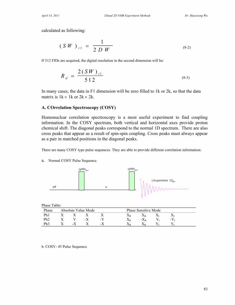
April 14, 2011 1Dand 2D NMR Experiment Methods Dr. Shaoxiong Wu
83
calculated as following:
( )S WD Wt 1
1
2 (8-2)
If 512 FIDs are acquired, the digital resolution in the second dimension will be:
RS W
dt
2
5 1 21( )
(8-3)
In many cases, the data in F1 dimension will be zero filled to 1k or 2k, so that the data matrix is 1k 1k or 2k 2k. A. COrrelation Spectroscopy (COSY) Homonuclear correlation spectroscopy is a most useful experiment to find coupling information. In the COSY spectrum, both vertical and horizontal axes provide proton chemical shift. The diagonal peaks correspond to the normal 1D spectrum. There are also cross peaks that appear as a result of spin-spin coupling. Cross peaks must always appear as a pair in matched positions in the diagonal peaks.
There are many COSY type pulse sequences. They are able to provide different correlation information:
a. Normal COSY Pulse Sequence.
Phase Table:
Phase Absolute Value Mode Phase Sensitive Mode Ph1 X X X X XR XR XI XI Ph2 X Y -X -Y XR -XR YI -YI Ph3 X -X X -X XR XR YI YI
b. COSY- 45 Pulse Sequence.
(Acquisition t2)ph3
pd
(p90)ph1
t1
(p90)ph2
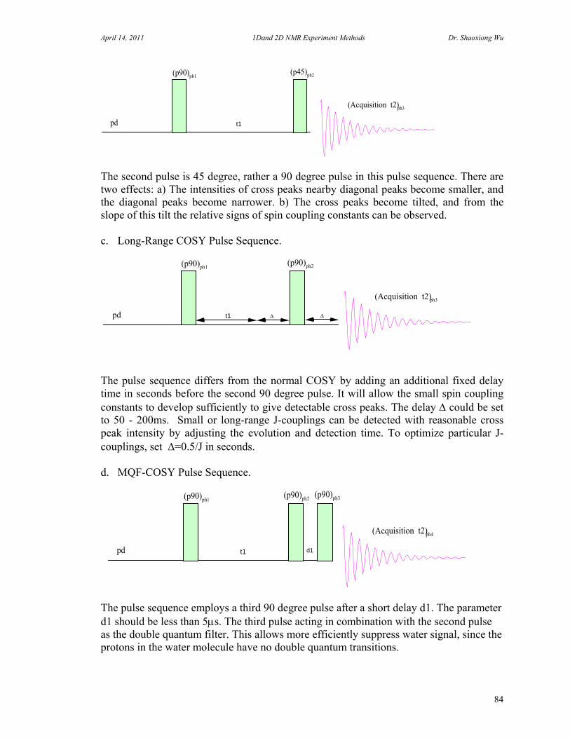
April 14, 2011 1Dand 2D NMR Experiment Methods Dr. Shaoxiong Wu
84
The second pulse is 45 degree, rather a 90 degree pulse in this pulse sequence. There are two effects: a) The intensities of cross peaks nearby diagonal peaks become smaller, and the diagonal peaks become narrower. b) The cross peaks become tilted, and from the slope of this tilt the relative signs of spin coupling constants can be observed.
c. Long-Range COSY Pulse Sequence.
The pulse sequence differs from the normal COSY by adding an additional fixed delay time in seconds before the second 90 degree pulse. It will allow the small spin coupling constants to develop sufficiently to give detectable cross peaks. The delay could be set to 50 - 200ms. Small or long-range J-couplings can be detected with reasonable cross peak intensity by adjusting the evolution and detection time. To optimize particular J-couplings, set =0.5/J in seconds. d. MQF-COSY Pulse Sequence.
The pulse sequence employs a third 90 degree pulse after a short delay d1. The parameter d1 should be less than 5s. The third pulse acting in combination with the second pulse as the double quantum filter. This allows more efficiently suppress water signal, since the protons in the water molecule have no double quantum transitions.
(Acquisition t2)ph3
pd
(p90)ph1
t1
(p45)ph2
(Acquisition t2)ph3
pd
(p90)ph1
t1
(p90)ph2
(Acquisition t2)ph4
pd
(p90)ph1
t1
(p90)ph2(p90)ph3
d1

April 14, 2011 1Dand 2D NMR Experiment Methods Dr. Shaoxiong Wu
85
Phase Table: Phase Magnitude Mode with DQF Ph1 X Y -X -Y X X -X -Y Ph2 X Y -X -Y Y X -Y X Ph3 X X X X Y Y Y Y Ph4 X -X X -X X -Y -X X
There are many interesting details about how to perform these experiments. If you are not familiar this experiment, you may follow the procedure to get a COSY spectrum with a standard sample, then try to take the COSY spectrum with your sample.
1. Take a normal proton 1D spectrum for the standard sample as a reference and set spectrum width.
2. Use 1puls sequence to calibrate the 90 degree pulse on your sample. 3. Set up the parameters:
2k data point in F2; 512 data point in F1; spectrum width: sw1=sw2; pulse delay set to 2 seconds; set the dummy scan to 4.
4. Processing the COSY data with magnitude mode. Final spectrum may be
symmetrized.
N
O
N1
2
3
4
8
7
13
17
H5
6
16
H
HH
H
9 HH
O
18
20
22
23
11
10
15
14
12
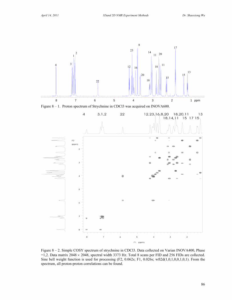
April 14, 2011 1Dand 2D NMR Experiment Methods Dr. Shaoxiong Wu
86
8 7 6 5 4 3 2 1 ppm
Figure 8 – 1. Proton spectrum of Strychnine in CDCl3 was acquired on INOVA600.
Figure 8 – 2. Simple COSY spectrum of strychnine in CDCl3. Data collected on Varian INOVA400, Phase =1,2. Data matrix 2048 2048, spectral width 3373 Hz. Total 8 scans per FID and 256 FIDs are collected. Sine bell weight function is used for processing (F2, 0.062s; F1, 0.026s; wft2d(1,0,1,0,0,1,0,1). From the spectrum, all proton-proton correlations can be found.
1315
17
15
11
20
18
1114
18
20
8
16
23
12
22
2 1
3 4
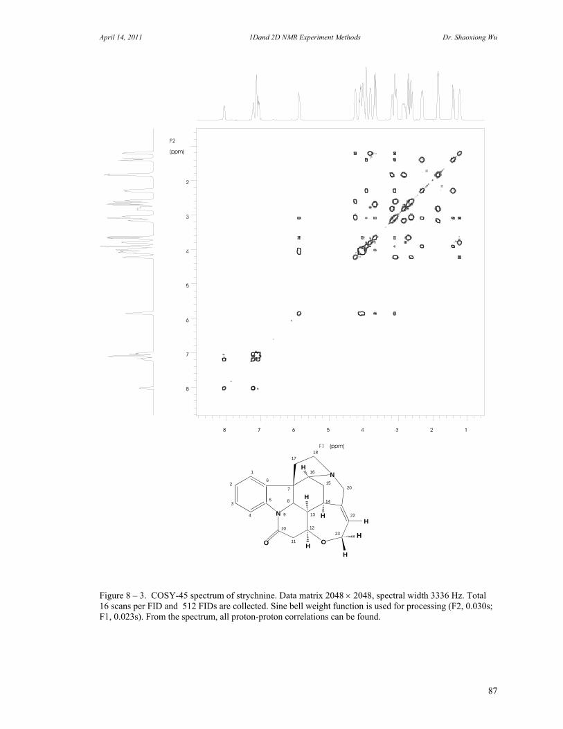
April 14, 2011 1Dand 2D NMR Experiment Methods Dr. Shaoxiong Wu
87
Figure 8 – 3. COSY-45 spectrum of strychnine. Data matrix 2048 2048, spectral width 3336 Hz. Total 16 scans per FID and 512 FIDs are collected. Sine bell weight function is used for processing (F2, 0.030s; F1, 0.023s). From the spectrum, all proton-proton correlations can be found.
N
O
N1
2
3
4
8
7
13
17
H5
6
16
H
HH
H
9 HH
O
18
20
22
23
11
10
15
14
12

April 14, 2011 1Dand 2D NMR Experiment Methods Dr. Shaoxiong Wu
88
Figure 8 – 4. Long-range COSY spectrum of Strychnine in CDCl3. Data matrix 2048 2048, spectral width 3336 Hz. Total 32 scans per FID and 512 FIDs are collected. The long-range delay is set to 300ms. Sine bell weight function is used for processing (F2, 0.077s; F1, 0.038s). From the spectrum, the four-bond couplings are enhanced.
(Acquisition t2)ph3
pd
(p90)ph1
t1
(p90)ph2

April 14, 2011 1Dand 2D NMR Experiment Methods Dr. Shaoxiong Wu
89
Figure 8 – 5. Double Quantum Filter COSY spectrum of Strychnine in CDCl3. Data matrix 2048 2048, spectral width 3336 Hz. Total 32 scans per FID and 512 FIDs are collected. Sine bell weight function is used for processing (F2, 0.077s; F1, 0.038s).
(Acquisition t2)ph4
pd
(p90)ph1
t1
(p90)ph2(p90)ph3
d1

April 14, 2011 1Dand 2D NMR Experiment Methods Dr. Shaoxiong Wu
90
COSY is the simplest 2D experiment. We could consider a spin system of two protons that are J-coupled (in Hz) and have different chemical shifts (in ppm). The first 90 degree pulse flips magnetization into XY rotating plane. Then the chemical shift develops during the t1 (F2 dimension). After the time t1, another 90 degree pulse applied, this allows the transform of antiphase magnetization of proton A with respect to proton B into antiphase magnetization of proton B with respect to proton A. It will show cross peaks between these two protons. If a proton is not J-coupled to other protons, this transform will be itself, so there is no cross peak. What can go wrong with COSY?
1. Artifacts? Symmetrize the spectra after Fourier Transform. You may set the delay longer at least 1.5 times of the longest T1.
2. Projection looks different than 1D proton spectrum Aliasing or folded in. You may check the spectrum width in both dimensions.
3. Peaks aren't resolved. Shimming problem or poor resolution. You may increase block size.
4. Peaks near the diagonal can't be seen. Use cosy-45. Check the T1 noise. Tips for acquiring a good COSY spectrum:
1. Use VT to control the sample temperature. 2. Do not spin the sample. 3. Set the gain to 70% of maximum gain for the sample. 4. Use at least 8 scan per FID, if gradient pulse is not used. 5. Make sure the probe is tuned for you sample and the 90 degree pulse is calibrated. 6. Set the correct spectrum width. Leave about 0.5 ppm at each side of the spectrum.

April 14, 2011 1Dand 2D NMR Experiment Methods Dr. Shaoxiong Wu
91
B. Heteronuclear Correlation Spectroscopy (HETCOR) The principles of HETCOR are precisely analogous to COSY. A different experimental regime however is required since two observing nuclei with different Larmor frequencies are involved. That is why this technique is refer to H, X-COSY, where X could be 13C, 15N, 31P, 29Si etc. The experiment is used to correlate the chemical shifts of X-nuclei with the chemical shifts of protons coupled with the X-nuclei. The assignment of one member of a spin-coupled pair leads immediately to the assignment of the other. Most NMR instruments with two channels can perform the experiment. The 90 degree pulses for X nucleus and proton need to be calibrated.
Figure 8 – 6. HETCOR pulse sequence. Where d90 specifies the proton 90 degree pulse, p90 is X nucleus
90 degree pulse and d1 and d2 are calculated from the J coupling constant. d1 = 1/(4* JXH) and d2 = 1/(3*
JXH). The ldlev is the decoupler power level. The t1 is the evolution time. There are many interesting details about how to perform this experiment. You may follow the procedure to get a HETCOR spectrum from a standard sample.
1. Take a normal proton 1D spectrum of carbon and proton for the sample as a reference
and set the spectrum width for both nuclei. 2. Use 1puls sequence to calibrate 90 degree pulse for carbon and 90 degree pulse for
the decoupler, i.e. proton channel. In some cases, you may have to tune the probe for both channels with your sample.
3. Run a DEPT spectrum to confirm the parameters. See the detailed instruction of
DEPT experiment. If DEPT does not work, HETCOR probably will not work either. Since this experiment relies on polarization transfer between proton and carbon, both carbon and proton 90 degree pulses should be correct.
4. Set up the HECOR experiment. The number of scans should multiple of 4. The JCH value should be set to the average of J-coupling constants of all CH, CH2 and CH3. The pulse delay could be set to two times of proton T1.
Acquisition t2
pd
p180
t1/2
p90
d90
1 H
X
d90t1/2
d1
d2
ldlev
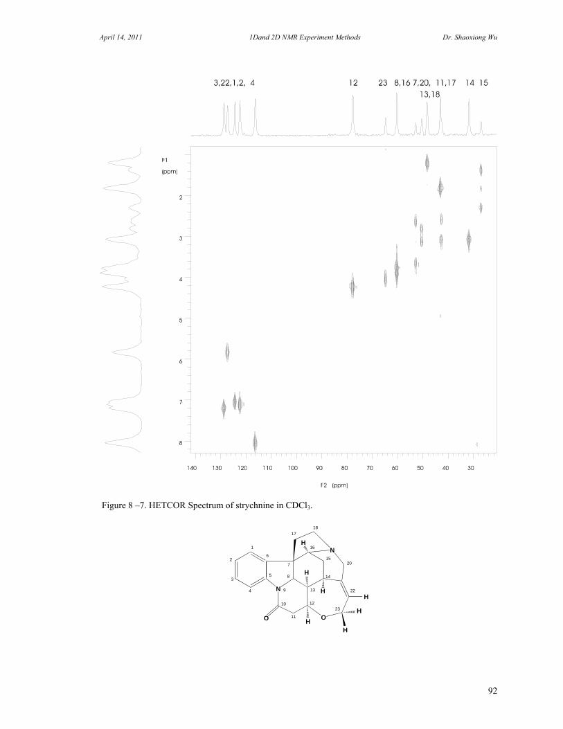
April 14, 2011 1Dand 2D NMR Experiment Methods Dr. Shaoxiong Wu
92
Figure 8 –7. HETCOR Spectrum of strychnine in CDCl3.
N
O
N1
2
3
4
8
7
13
17
H5
6
16
H
HH
H
9 HH
O
18
20
22
23
11
10
15
14
12

April 14, 2011 1Dand 2D NMR Experiment Methods Dr. Shaoxiong Wu
93
C. Nuclear Overhauser and Exchange Spectroscopy (NOESY) This technique is developed to observe NOE in the two dimensional spectroscopy. The NOEs between all spatially close protons can he observed as cross peaks simultaneously. It is very important and useful technique in molecular structure elucidation and molecular conformation determination. The experiment NOESY yields a pure adsorption correlation map on the basis of incoherent magnetization transfer processes such as dipolar coupling and chemical exchange. The incoherent magnetization transfer happens during the mixing time that should be properly set so that the maximum NOE could be observed. The pulse sequence consists of three 90 degree pulses. The first pulse creates transverse magnetization, the magnetization is then frequency labeled during the evolution time. The second pulse flips the labeled components to -z axis. These components are mixed through cross relaxation processes during the mixing time. The last composite 90 degree pulse rotates the magnetization to transverse plane again for observation.
Figure 8 – 8. Where p90 specifies the proton 90 degree pulse The F2 is homonuclear decoupling channel for eliminating the water signal. In most cases, only Fl channel is used. The mixing time is about 50ms to 400ms and depends on the molecule size and solvent. Experiment Procedure: 1. Take a normal proton 1D spectrum as a reference and set spectrum width. 2. Use one pulse sequence to calibrate 90 degree pulse for proton. 3. Set NOESY experiment parameters: set mixing time to 200ms; set data matrix to 2048
512; set number of scans to 32. 4. Adjust parameters to get a flat base line with first order baseline correction equal to zero correction. 5. Turn the spinner off for a better quality spectrum. Use VT control.
Acquisition t2
pd
p90
t1
p90 comp90
Mix
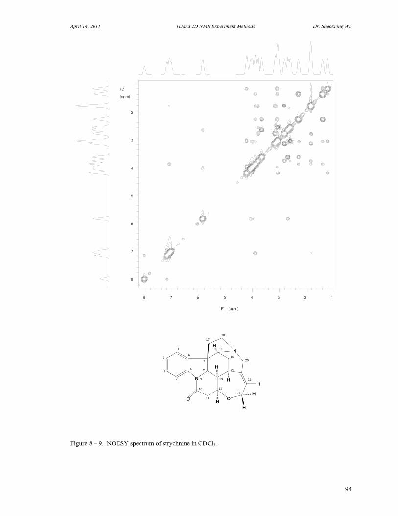
April 14, 2011 1Dand 2D NMR Experiment Methods Dr. Shaoxiong Wu
94
Figure 8 – 9. NOESY spectrum of strychnine in CDCl3.
N
O
N1
2
3
4
8
7
13
17
H5
6
16
H
HH
H
9 HH
O
18
20
22
23
11
10
15
14
12

April 14, 2011 1Dand 2D NMR Experiment Methods Dr. Shaoxiong Wu
95
D. Rotating Frame Overhauser Effect Spectroscopy (ROESY) Nuclear Overhauser Effect (NOE) has been widely used in structure determination. With high field NMR spectrometer, the detection of NOE by NOESY is sometimes quite difficult when the molecule weight is in the order of 1000 to 2000, since the NOE effect changes its sign depending on the molecular correlation time. When molecules have a motional correlation time near the condition 0c= 1, where 0 is Larmor frequency and c is correlation time, no NOE will be observed. When 0c > 1, as in the case of macromolecule, the NOE approaches -1 and specificity is lost due to spin diffusion. The ROESY experiment with spin lock in the rotating frame is particularly suited for overcoming these difficulties since ROESY enhancement is always positive and increases monotonically with 0c. In the ROESY spectrum, NOE peaks appear in a positive phase and diagonal peaks have negative phase; however, for chemically or conformationally exchanging protons the cross peaks will have a negative phase. The pulse sequence of ROESY is analogous to that of HOHAHA (HOmonuclear HArtmann HAhn). The required spin lock time is dependent on the size of the molecule and usually about 200 ms. The pulse scheme of the phase sensitive ROESY with hypercomplex phase cycling is shown in the following figure. The pulse sequence begins with a relaxation delay, and is followed by a pre-saturation pulse to eliminate the big solvent peak. At the end of saturation period, a 90 degree pulse flips the magnetization to Y axis, spins will precess under their chemical shifts during the evolution time. Then a strong RF field is turned on for duration of mixing period, during which spin exchange takes place along the spin locked axis.
Figure 8 – 10. Where presat specifies the pre-saturation time and spin lock is the interval of the spin lock.
The spin lock power is normally set to 3000Hz, about 10 ppm for a 600 MHz instrument.
There are two different types of spurious cross peaks occasionally appearing in a ROESY spectrum. Both of them are due to coherence transfer between scalar coupled spins. The first type is called COSY-type cross peak induced by the fact that the long spin lock pulse also acts as a mixing pulse for anti-phase magnetization, analogous to the 90 degree mixing pulse in the COSY experiment. Placing the carrier frequency away from the center of the spectrum can eliminate this type of artifact. The second type is due to Hartmann Hahn transfer through scalar coupling between mutually coupled protons. Note the Hartmann Hahn cross peaks will have the same phase as the diagonal peaks, whereas the ROESY cross peaks have opposite phase. This type of artifact can he eliminated by
Acquisition t2
pd t1
p90
Spin Lock
Pre-saturation
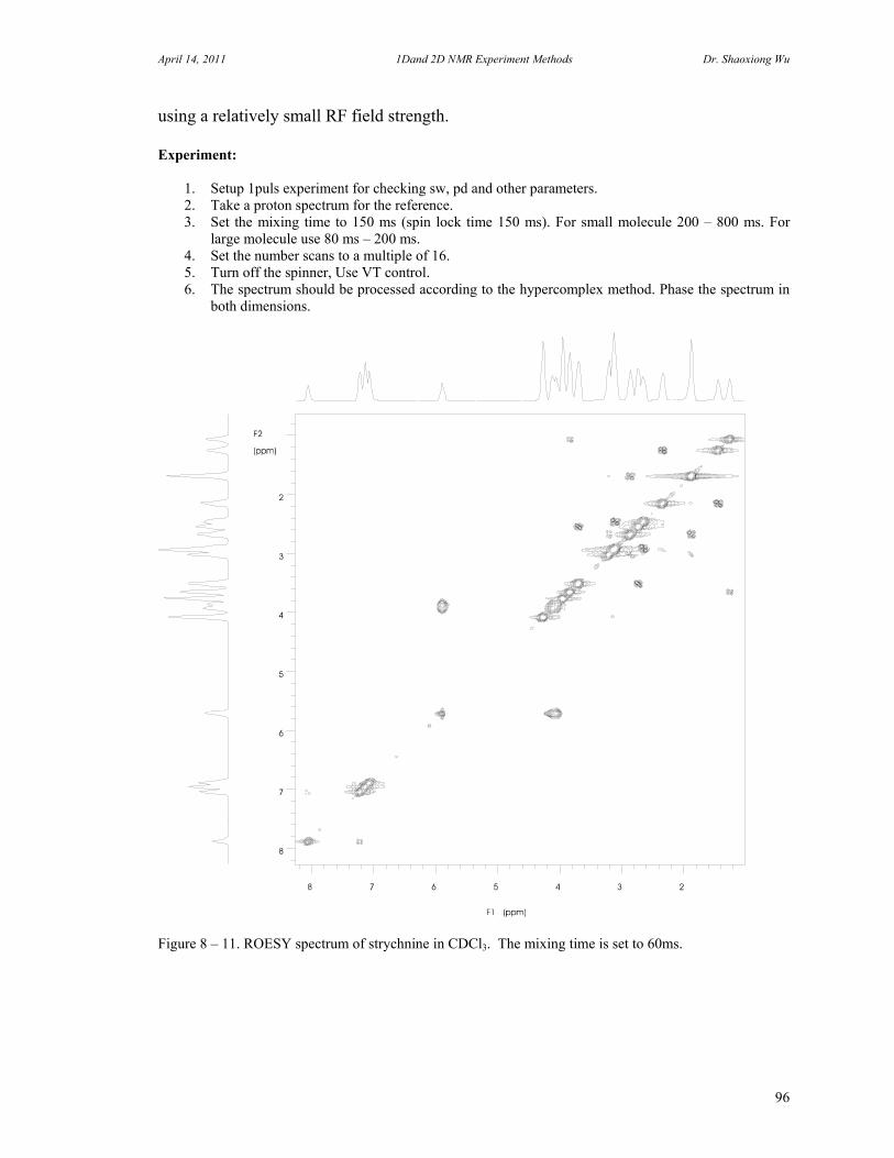
April 14, 2011 1Dand 2D NMR Experiment Methods Dr. Shaoxiong Wu
96
using a relatively small RF field strength. Experiment:
1. Setup 1puls experiment for checking sw, pd and other parameters. 2. Take a proton spectrum for the reference. 3. Set the mixing time to 150 ms (spin lock time 150 ms). For small molecule 200 – 800 ms. For
large molecule use 80 ms – 200 ms. 4. Set the number scans to a multiple of 16. 5. Turn off the spinner, Use VT control. 6. The spectrum should be processed according to the hypercomplex method. Phase the spectrum in
both dimensions.
Figure 8 – 11. ROESY spectrum of strychnine in CDCl3. The mixing time is set to 60ms.

April 14, 2011 1Dand 2D NMR Experiment Methods Dr. Shaoxiong Wu
97
E. Total Correlation Spectroscopy (TOCSY) TOtal Correlation SpectroscopY(TOCSY) is one of the principal experiments used in establishing connectivity between nuclei of scalar coupled spin systems. The experiment is designed to eliminate Zeeman contributions from the interactions of isotropically coupled spin systems. The method is based on the homonuclear cross polarization technique, i.e. by using an MLEV-17 pulse sequence to spin lock the magnetization to obtain polarization transfer. Under this condition, coherence migrates in an oscillatory manner throughout the entire spin system. This technique is therefor mostly used for peptides or oligosaccharides, since it could identify a single residue. For complex molecules, the resulting TOCSY spectrum provides a reliable identification of spin systems that cannot be resolved by other methods. A major advantage of TOCSY is that net magnetization transfer occurs and a phase sensitive 2D spectrum with all peaks in the absorption mode can be obtained.
Figure 8 – 12. Where the trim pulse set to 2 to 4 ms. MLEV-17 is a series of composite 180 degree pulses
(90-180-90). The pulse width is in the order of 40 s, corresponding to an effective spin-lock field of
7000Hz. The total length of spin lock time sets to 200 ms. The loop parameter must be an even number. Note: TOCSY experiment requires systems having linear amplifiers with computer controlled attenuators on the observe transmitter channel. Experiment: 1. Setup 1puls experiment for checking sw, pd and other parameters. Take a proton
spectrum for the reference. 2. Calibrate the “hard” 90 degree pulse. Use 95% or higher transmitter power available.
It should be in the range of 7 - 14 s. Calibrate the “soft” 90 degree pulse. Set the pulse width to 33-38 s (Corresponding to the spin-lock field strength of 7575 - 7142 Hz), then change the transmitter power to find the 90 degree pulse.
3. Set the spin lock to 30 - 200 ms depends on size of molecule under observation.
Set the trim pulse to 2ms at the same transmitter power as the spin-lock pulse. 4. Set the number scans to a multiple of 16. 5. Turn off the spinner. Use VT control.
Acquisition t2
pd t1
p90
Spin Lock
Pre-saturation
Trim PulseTrim Pulse
MLEV-17

April 14, 2011 1Dand 2D NMR Experiment Methods Dr. Shaoxiong Wu
98
6. The spectrum should be processed according to the hypercomplex method. Phase the
data in both dimensions.
Figure 8 – 13. TOCSY spectrum of strychnine in CDCl3 acquired on INOVA400. Data set 2048 256, zero-filled to 2048 1024 mixing time 50 ms, trim pulse 2 ms, spin-lock pulse width 33s.
N
O
N1
2
3
4
8
7
13
17
H5
6
16
H
HH
H
9 HH
O
18
20
22
23
11
10
15
14
12

April 14, 2011 1Dand 2D NMR Experiment Methods Dr. Shaoxiong Wu
99
F. Incredible Nature Abundance Double Quantum Transfer Experiment (INADEQUATE)
INADEQUATE is an NMR experiment of analyzing adjacent spin pairs from the correlation of double quantum transition and chemical shifts. Jc-c spin coupling constants are valuable for the structure elucidation of chemical compounds. However the Jc-c is much difficult to determine in nature abundance, since the amount of 13C in the nature is about 1% of 12C isotope, the probability of two 13C nuclei being adjacent is one out of ten thousand. In normal proton decoupled 13C spectra, almost of all carbon signals are those of isolated 13C. In this experiment the 13C signals from isolated 13Cs are suppressed and the coupled 13C (doublets, coupled to another 13C) are observed, so that the connectivity of carbons can be determined. The Experiment is extremely useful, but suffers from the low sensitivity. A very concentrated sample may be used. To judge whether an INADEQUATE experiment will be successful, you may run a normal decoupled 13C spectrum with one scan, the S/N should be 35:1 or better for 2D INADEQUATE and 5:1 for 1D INADEQUATE.
Figure 8 – 14. The pulse sequence uses 90 and 180 degree pulses. Extensive phase cycling is carried out to suppress the singlet 13C signals. JC-C is one bond carbon-carbon coupling constant. Experiment 1. Tune the probe. Calibrate 90 degree pulse. 2. Calibrate the decoupler. 3. Run Jcc 1D, make sure there is antiphase doublet for every carbon. 4. Run INADEQUATE. 4K x 64 and at least nt = 128 for a complete phase cycling. Note: There is a rule of thumb by that you could judge if the experiment will be successful. Run a normal 1D 13C spectrum with one scan using a 90 degree pulse with proper gain setting. If the S/N ratio is better than 30:1 you might be able to get a reasonable spectrum within 24 hours.
Proton Decoupling
p90
Acquisition t2
p180
1/4Jcc t1pd
p90 p90
1/4Jcc
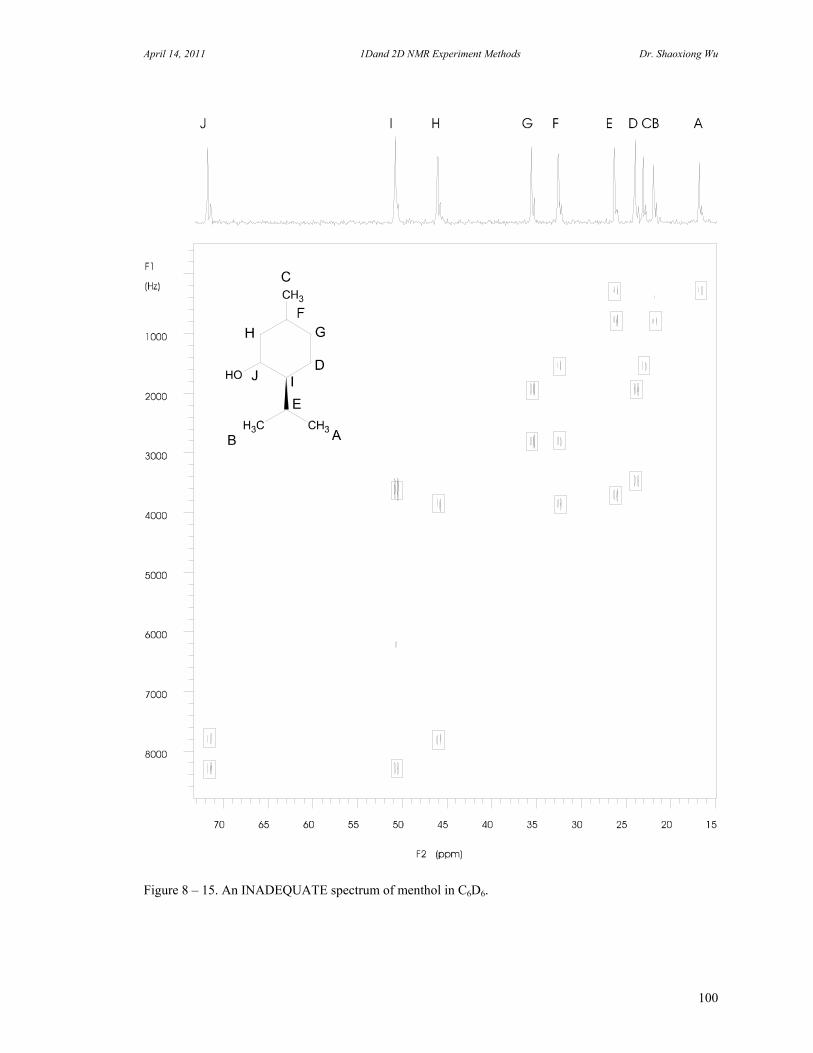
April 14, 2011 1Dand 2D NMR Experiment Methods Dr. Shaoxiong Wu
100
Figure 8 – 15. An INADEQUATE spectrum of menthol in C6D6.
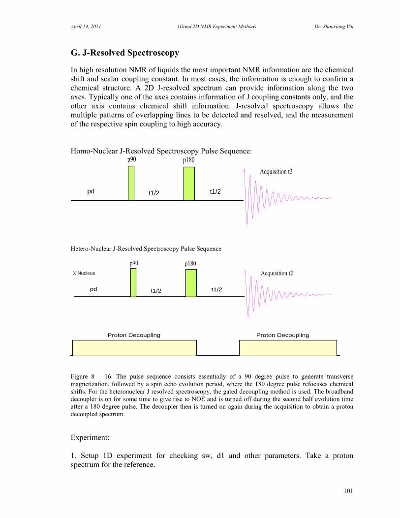
April 14, 2011 1Dand 2D NMR Experiment Methods Dr. Shaoxiong Wu
101
G. J-Resolved Spectroscopy In high resolution NMR of liquids the most important NMR information are the chemical shift and scalar coupling constant. In most cases, the information is enough to confirm a chemical structure. A 2D J-resolved spectrum can provide information along the two axes. Typically one of the axes contains information of J coupling constants only, and the other axis contains chemical shift information. J-resolved spectroscopy allows the multiple patterns of overlapping lines to be detected and resolved, and the measurement of the respective spin coupling to high accuracy. Homo-Nuclear J-Resolved Spectroscopy Pulse Sequence:
Hetero-Nuclear J-Resolved Spectroscopy Pulse Sequence
Figure 8 – 16. The pulse sequence consists essentially of a 90 degree pulse to generate transverse magnetization, followed by a spin echo evolution period, where the 180 degree pulse refocuses chemical shifts. For the heteronuclear J resolved spectroscopy, the gated decoupling method is used. The broadband decoupler is on for some time to give rise to NOE and is turned off during the second half evolution time after a 180 degree pulse. The decoupler then is turned on again during the acquisition to obtain a proton decoupled spectrum. Experiment: 1. Setup 1D experiment for checking sw, d1 and other parameters. Take a proton spectrum for the reference.
Acquisition t2
p180
t1/2pd
p90
t1/2
Proton Decoupling
Acquisition t2
p180
t1/2pd
p90
Proton Decoupling
t1/2
X Nucleus

April 14, 2011 1Dand 2D NMR Experiment Methods Dr. Shaoxiong Wu
102
2. Set the number scans to a multiple of 16. 3. The Spectrum should be processed according to the hypercomplex method. Phase the data in both directions.
Figure 8 – 17. Home nuclear 2D J-resolved spectrum of strychnine in CDCl3. Home nuclear 2D J-resolved spectroscopy is rarely used today. It has been mostly replaced by phase-sensitive DQCOSY. In many cases, this experiment is easy to perform and understand.
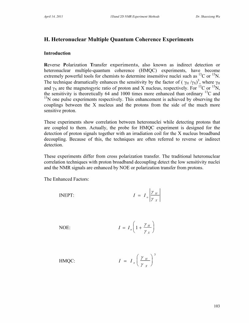
April 14, 2011 1Dand 2D NMR Experiment Methods Dr. Shaoxiong Wu
103
H. Heteronuclear Multiple Quantum Coherence Experiments Introduction Reverse Polarization Transfer experiments, also known as indirect detection or heteronuclear multiple-quantum coherence (HMQC) experiments, have become extremely powerful tools for chemists to determine insensitive nuclei such as 13C or 15N. The technique dramatically enhances the sensitivity by the factor of ( H /X)3, where H and X are the magnetogyric ratio of proton and X nucleus, respectively. For 13C or 15N, the sensitivity is theoretically 64 and 1000 times more enhanced than ordinary 13C and 15N one pulse experiments respectively. This enhancement is achieved by observing the couplings between the X nucleus and the protons from the side of the much more sensitive proton. These experiments show correlation between heteronuclei while detecting protons that are coupled to them. Actually, the probe for HMQC experiment is designed for the detection of proton signals together with an irradiation coil for the X nucleus broadband decoupling. Because of this, the techniques are often referred to reverse or indirect detection. These experiments differ from cross polarization transfer. The traditional heteronuclear correlation techniques with proton broadband decoupling detect the low sensitivity nuclei and the NMR signals are enhanced by NOE or polarization transfer from protons. The Enhanced Factors:
INEPT: I I oH
X
NOE: I I oH
X
1
HMQC: I I oH
X
3

April 14, 2011 1Dand 2D NMR Experiment Methods Dr. Shaoxiong Wu
104
Instrument and Probes The HMQC experiments require the instruments are capable of generating pulse on 1H and X and possibly decoupling X while observing 1H. All high field NMR instruments should have dual broadband system. The frequencies of both observe and decoupling channels could be set to 1H to 103Rh or lower. Performing an indirect detection experiment simply involves setting the observe channel to observe proton and the decoupling channel to decouple X nucleus. It also requires that the decoupler power can fast switch between high power output for the hard pulse and low power output for the broad band decoupling. Some of old instrument do not have this capability, but it still can perform HMQC experiments without decoupling. The most commonly used probe for HMQC experiments is an RPT probe (Reverse Polarization Transfer Probe) or ID probe (Indirect Detection probe) that has a 1H observe coil and a tunable X nucleus decoupling coil, and typically has the 1H observe coil closer to the sample tube for the highest possible sensitivity of the observed nucleus. Normal broadband probes also have a 1H coil used for proton decoupling and an X nucleus observe coil. It can be used for HMQC experiments too, but it has comparatively lower sensitivity than RPT probe, since the 1H observe coil is an outer coil. It will, however, provide some sensitivity improvement over direct detection heteronuclear correlation experiments. Pulse Sequences The essence of the HMQC experiment is the cancellation or elimination of the signals from proton attached to 12C, leaving only signals from protons attached to 13Cs contribute to a 13C -1H chemical shift correlation spectrum. There are several pulse sequences available: 1. Reverse detected heteronuclear coherence sequence for single channel decoupler
system.
A c q u i s i t i o n t 2
p d
p 1 8 0p 9 0
d 9 0
1 H
Xd 9 0
d 1d 11 /2 J X H

April 14, 2011 1Dand 2D NMR Experiment Methods Dr. Shaoxiong Wu
105
Figure 8 – 18. HMQC pulse sequence without X decoupling during the acquisition time.
Figure 8 – 19. HMQC pulse sequence with X decoupling during the acquisition time. 2. Phase-Sensitive HMQC with BIRD Selection and GARP Decoupling
Figure 8 –20. HMQC pulse sequence with BIRD selection with X decoupling.
Re-cabling for HMQC experiments
The following is the essential configuration for HMQC experiment. It can be directly used for calibrating 90 degree pulse of the X nucleus by the one pulse experiment. The filter is band-pass filter that depends on the frequency of X nucleus. In the lock channel line, install a 2H band-pass filter. After the filter is installed, the lock phase is expected to be change. This filter can be left in the system at all times; it will, however, cause a small loss in lock sensitivity (about 3 dB).
Acquisition t2
pd
p180p90
d90
1H
Xd90
d 1
ldlev
d 11/ 2J XH
A cqu is i tion t2
pd
p1 80p9 0
d9 0 d9 0X
d 18 0
1H
t1 /2 t
1 / 2
p 18 0 p 90 p9 0
X D e co u p ling

April 14, 2011 1Dand 2D NMR Experiment Methods Dr. Shaoxiong Wu
106
In the 1H channel (observe channel), install a proton high-pass filter. In the X channel (decoupler channel), install an X-nucleus band-pass filter and 1H low-pass filter.
Figure 8 – 21. Probe interface for HMQC experiments on an INOVA600 NMR instrument. The red doted line is for routine X observe experiments. Experiment Conditions: Because of involving cancellation of the signal from the proton bounded to 12C, the HMQC experiment is critically dependent on this cancellation efficiency. Several of experimental conditions could influence the quality of spectrum.
1. Put filters in the lines. Although they will cause power loss, interference between proton and X nucleus decoupling can be eliminated. Especially, using a 2H band-pass filter will eliminate the influence by decoupling pulse that can affect the lock and cause field instabilities.
2. Use VT operation and be sure the system is in the thermal equilibrium when you calibrate all these parameters. Performing experiment with X nucleus decoupling, you will apply large amount of power to the probe, the temperature of the probe and sample may vary during the experiment.
XMTR
Probe
Output Output
XMTR
Probe
1/4 wavelength
005
0 8+ +
--
Tune
LOCK
PROTON X CHANNEL
VT Air Input
1H Tune X Tune
Ext. Capacitor
VT Cable
Coling Air
Broad Band Channel from Console
High Band Channel From Console
To High Band Receiver
To BB Receiver
Normal Broad Band ObserveHMQC Exp.
HMQC Exp. Normal Broad Band Observe

April 14, 2011 1Dand 2D NMR Experiment Methods Dr. Shaoxiong Wu
107
3. Use large number of acquisition (nt > 32). Both cancellation and S/N will be improved.
4. Minimize floor vibration. An anti-vibration system should be installed. Run experiment on weekend. Turn the spinner off.
5. On the Systems that do not have linear amplifiers, if the amplifier is left on for too long for decoupling 13C or other nuclei, the voltage of the power supply droops and causes system parameters changes or it may burn the amplifier. To solve this problem, it is suggested that performing experiments without X nucleus decoupling during the acquisition or limiting left decoupling power on less than 50 ms which may be long enough for the acquisition time.
1H-13C HMQC Experiments Setup
1. Obtain a normal 1H spectrum of the standard sample (1% 13CH3I in CDC13) by one pulse direct detection mode. The large three-line (approximately 1:1:1 ) illustrated in the following spectrum will be observed. The central line at 2.2 ppm represents the 1H-12C protons of CH3I and the outer two lines are 1H-13C protons of 13CH3I. The peaks centered at 1.2 ppm in the spectrum are 13C enriched impurity peaks. The peaks near 3.7 ppm are trimethylphosphite, which is also present in the sample for 31p indirect detection experiments. In this experiment we are interested in the peaks at 2.2 ppm only.
Figure 8 – 22. Normal proton spectrum of 1% 13CH3I in CDC13.
2. Obtain a normal 13C spectrum of the standard sample as a reference. The 13C signal from 13CH3I is extremely far upfield ( -22.3 ppm). Two peaks at l0 ppm present the trimethylphosphite and a triplet at 77 ppm is the CDC13.
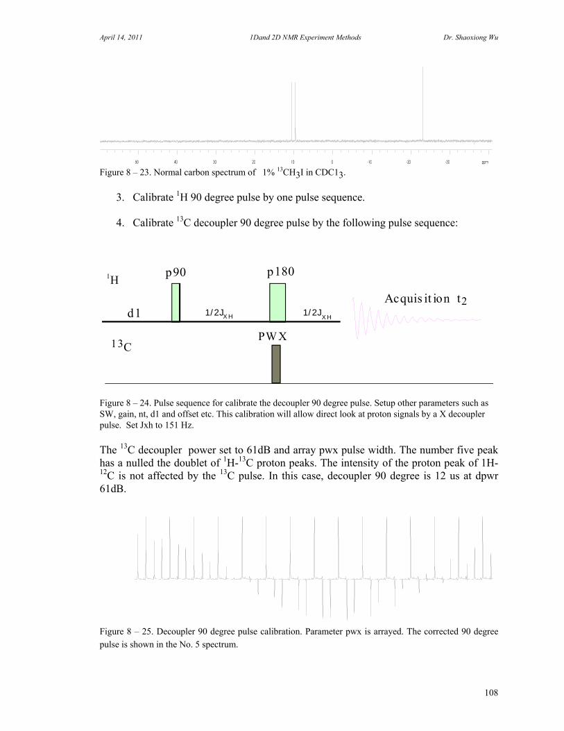
April 14, 2011 1Dand 2D NMR Experiment Methods Dr. Shaoxiong Wu
108
Figure 8 – 23. Normal carbon spectrum of 1% 13CH3I in CDC13.
3. Calibrate 1H 90 degree pulse by one pulse sequence.
4. Calibrate 13C decoupler 90 degree pulse by the following pulse sequence:
Figure 8 – 24. Pulse sequence for calibrate the decoupler 90 degree pulse. Setup other parameters such as SW, gain, nt, d1 and offset etc. This calibration will allow direct look at proton signals by a X decoupler pulse. Set Jxh to 151 Hz. The 13C decoupler power set to 61dB and array pwx pulse width. The number five peak has a nulled the doublet of 1H-13C proton peaks. The intensity of the proton peak of 1H-12C is not affected by the 13C pulse. In this case, decoupler 90 degree is 12 us at dpwr 61dB.
Figure 8 – 25. Decoupler 90 degree pulse calibration. Parameter pwx is arrayed. The corrected 90 degree
pulse is shown in the No. 5 spectrum.
Acquis it ion t2d1
p180p901H
13CPW X
1/2JX H 1/2JX H

April 14, 2011 1Dand 2D NMR Experiment Methods Dr. Shaoxiong Wu
109
5. The following spectra show how the phase is affected by the parameter Jxh. From the left to the right Jxh: 100,120,140,160,180,200,220,240 Hz. In most case, it should set to the average of Jxh of the sample.
Figure 8 – 26. Parameter jxh is arrayed. The corrected jxh is shown in the No. 4 spectrum.
6. Run 1D HMQC pulse sequence. The doublet should be shown and a null signal is for 1H-12C protons.
Figure 8 – 27. 1D HMQC spectrum with carbon decoupler off.
7. Run HMQC with decoupling power on for the standard.
Figure 8 – 28. 1D HMQC spectrum with carbon decoupler on.
8. Run 2D HMQC pulse sequence. Set ni = 128. Turn the decoupler power off.
3 . 5 3 . 0 2 . 5 2 . 0 1 . 5 1 . 0 p p m
3 . 5 3 . 0 2 . 5 2 . 0 1 . 5 1 . 0 p p m
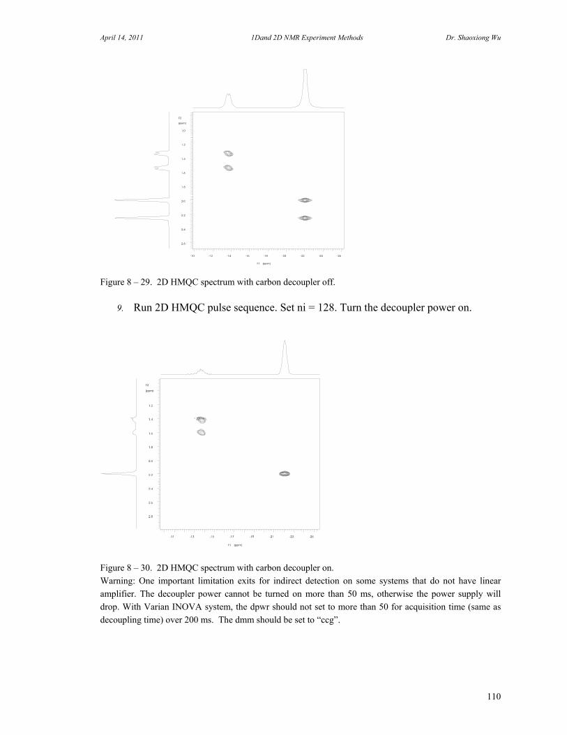
April 14, 2011 1Dand 2D NMR Experiment Methods Dr. Shaoxiong Wu
110
Figure 8 – 29. 2D HMQC spectrum with carbon decoupler off.
9. Run 2D HMQC pulse sequence. Set ni = 128. Turn the decoupler power on.
Figure 8 – 30. 2D HMQC spectrum with carbon decoupler on.
Warning: One important limitation exits for indirect detection on some systems that do not have linear
amplifier. The decoupler power cannot be turned on more than 50 ms, otherwise the power supply will
drop. With Varian INOVA system, the dpwr should not set to more than 50 for acquisition time (same as
decoupling time) over 200 ms. The dmm should be set to “ccg”.
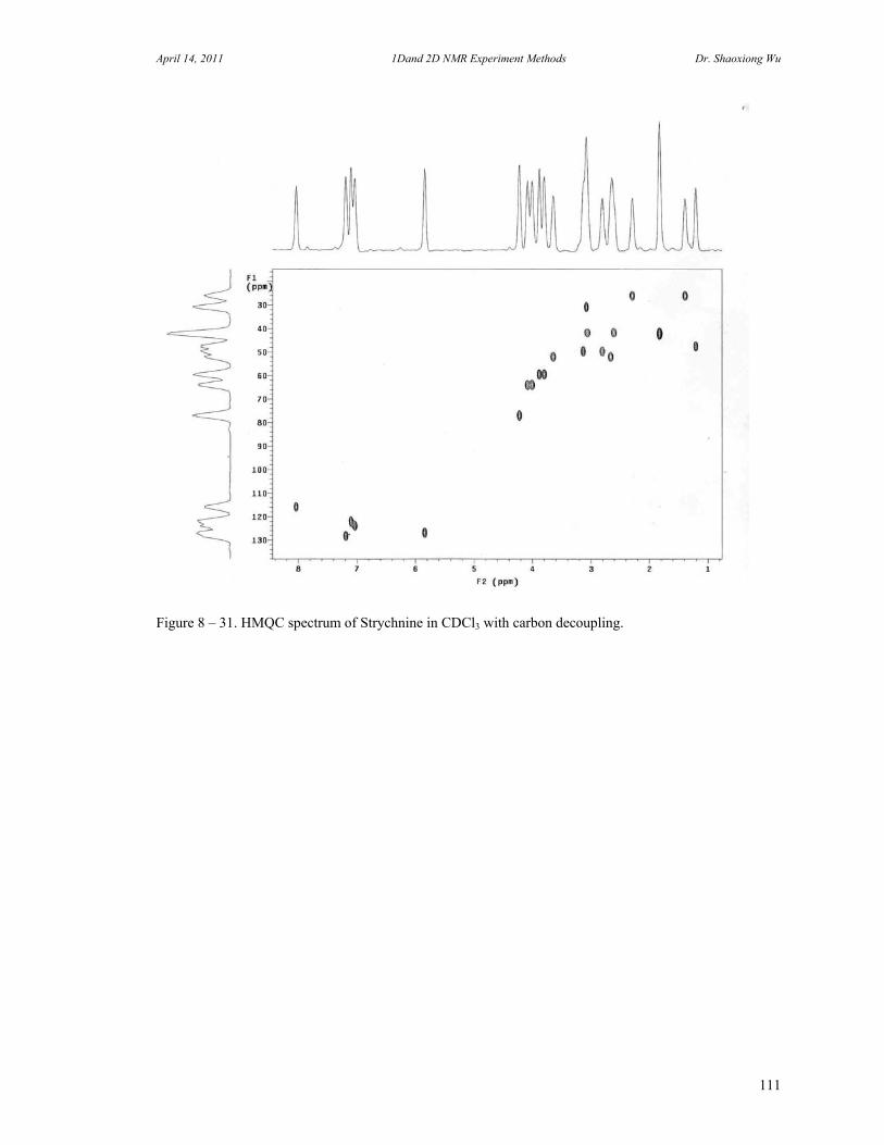
April 14, 2011 1Dand 2D NMR Experiment Methods Dr. Shaoxiong Wu
111
Figure 8 – 31. HMQC spectrum of Strychnine in CDCl3 with carbon decoupling.
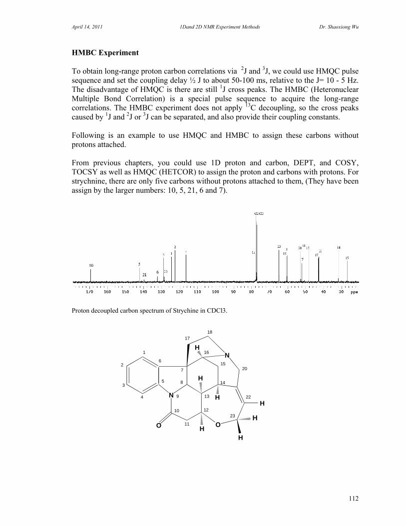
April 14, 2011 1Dand 2D NMR Experiment Methods Dr. Shaoxiong Wu
112
HMBC Experiment To obtain long-range proton carbon correlations via 2J and 3J, we could use HMQC pulse sequence and set the coupling delay ½ J to about 50-100 ms, relative to the J= 10 - 5 Hz. The disadvantage of HMQC is there are still 1J cross peaks. The HMBC (Heteronuclear Multiple Bond Correlation) is a special pulse sequence to acquire the long-range correlations. The HMBC experiment does not apply 13C decoupling, so the cross peaks caused by 1J and 2J or 3J can be separated, and also provide their coupling constants. Following is an example to use HMQC and HMBC to assign these carbons without protons attached. From previous chapters, you could use 1D proton and carbon, DEPT, and COSY, TOCSY as well as HMQC (HETCOR) to assign the proton and carbons with protons. For strychnine, there are only five carbons without protons attached to them, (They have been assign by the larger numbers: 10, 5, 21, 6 and 7).
Proton decoupled carbon spectrum of Strychine in CDCl3.
N
O
N1
2
3
4
8
7
13
17
H5
6
16
H
HH
H
9 HH
O
18
20
22
23
11
10
15
14
12
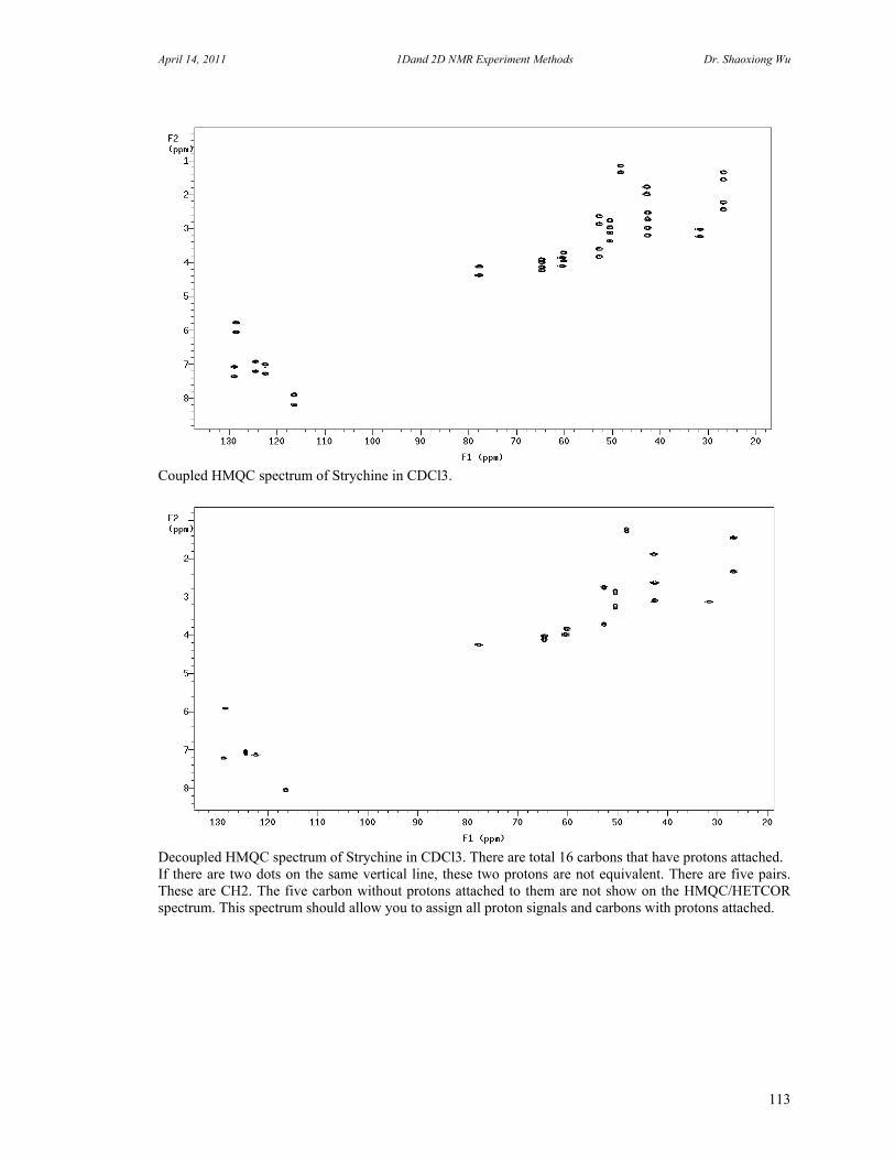
April 14, 2011 1Dand 2D NMR Experiment Methods Dr. Shaoxiong Wu
113
Coupled HMQC spectrum of Strychine in CDCl3.
Decoupled HMQC spectrum of Strychine in CDCl3. There are total 16 carbons that have protons attached. If there are two dots on the same vertical line, these two protons are not equivalent. There are five pairs. These are CH2. The five carbon without protons attached to them are not show on the HMQC/HETCOR spectrum. This spectrum should allow you to assign all proton signals and carbons with protons attached.
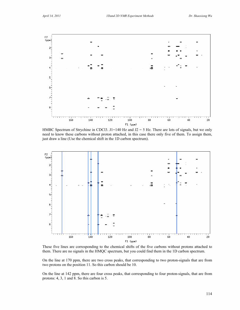
April 14, 2011 1Dand 2D NMR Experiment Methods Dr. Shaoxiong Wu
114
HMBC Spectrum of Strychine in CDCl3. J1=140 Hz and J2 = 5 Hz. There are lots of signals, but we only need to know these carbons without proton attached, in this case there only five of them. To assign them, just draw a line (Use the chemical shift in the 1D carbon spectrum).
These five lines are corresponding to the chemical shifts of the five carbons without protons attached to them. There are no signals in the HMQC spectrum, but you could find them in the 1D carbon spectrum. On the line at 170 ppm, there are two cross peaks, that corresponding to two proton-signals that are from two protons on the position 11. So this carbon should be 10. On the line at 142 ppm, there are four cross peaks, that corresponding to four proton-signals, that are from protons: 4, 3, 1 and 8. So this carbon is 5.

April 14, 2011 1Dand 2D NMR Experiment Methods Dr. Shaoxiong Wu
115
On the line at 132 ppm, there are three cross peaks, that corresponding to three proton-signals, that are from 4, 2, and 8. So this carbon is 6.
These two carbons are alike. We do see the signals from proton 1 and 17 to carbon 6, but the signals are very small. The good evidence is the proton signal 3 to carbon 5, rather than carbon 6, that is equivalent to proton 2 to carbon 6. On the line at 140 ppm, there are five cross peaks, that are corresponding to five proton-signals, that are from protons at 23, 20 and 15, so this is the carbon 21. On the line at 51 ppm, there are four cross peaks, that are corresponding to four proton-signals, that are from protons at 1, 8 , 15 and 17, so this is the carbon 7. We did not see the cross peak from proton 16 to carbon 7, because the 2JCH coupling is about 2 Hz. The cross peak is too small to see. In many cases, one HMBC spectrum is enough to sign these none-protonated carbons, but in some molecule, we may have to take more HMBC experiments by change different value of 1JCH and 2JCH, to enhance signals we like to observe.

April 14, 2011 1Dand 2D NMR Experiment Methods Dr. Shaoxiong Wu
116
9. NMR Auxiliary Reagents and Applications A. Chemical Shift Reagents There is a larger amount of paramagnetic compounds that, when added to a NMR solvent, can lead to large changes in the chemical shifts of the sample’s nuclei. These compounds are coordination complexes of paramagnetic metal ions of the lanthanide group, such as europium (Eu3+), Ytterbium (Yb3+) and praseodymium (Pr3+). One commercially available chemical shift reagent, Eurpium (III) perdeutero-tris (1,1,1,2,2,3,3-Heptafluoro-7,7-dimethyl-4,6-octanrdionate) has an Eu3+ ion coordinated to three equivalent -diketone enolates. When a small amount of chemical shift reagent added to an NMR solution, there is rapid reversible complexation between the reagent and the sample molecules. The sample molecules in the complex are held in relatively close to the paramagnetic metal ion and experience the strong deshielding, causing a downfield chemical shift from their original positions. The nuclei nearest to the paramagnetic ion will have a largest shift. This interaction is called pseudocontact shift affect, which operates directly through space, rather than through bond. Its magnitude is inversely proportional to the cube of the average distance from the metal ion to the nucleus of interest. The magnitude of chemical shift is also a function of the equilibrium constant for complexation as well as the mole ration of reagent to sample. But since complexation equilibrium constant K is normally greater than one, the chemical shift will stop to move as the ratio of reagent to sample approaches one to one. Beyond that ratio, each sample molecule already has its own metal complex; so additional amount of chemical shift reagent has little effect on the peak position.
It is abbreviated Eu(FOD)3. This compound is available in both protonated and deuterated version. See http://www.wilmad.com
O
NO
CH3
O
OO
O
CH3CH3
CH3
H
HH
H
H
H
20
45
18',18'
6
7 6 5 4 3 2 1 ppm
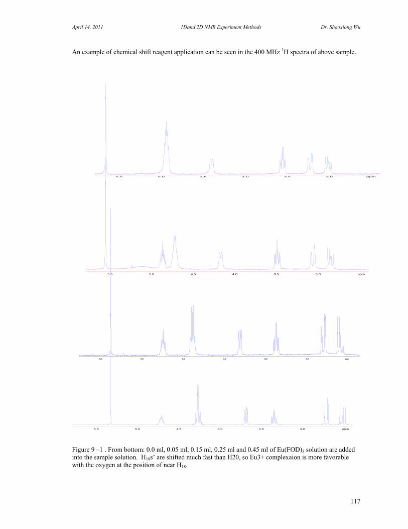
April 14, 2011 1Dand 2D NMR Experiment Methods Dr. Shaoxiong Wu
117
An example of chemical shift reagent application can be seen in the 400 MHz 1H spectra of above sample.
Figure 9 –1 . From bottom: 0.0 ml, 0.05 ml, 0.15 ml, 0.25 ml and 0.45 ml of Eu(FOD)3 solution are added into the sample solution. H18s’ are shifted much fast than H20, so Eu3+ complexaion is more favorable with the oxygen at the position of near H18.
5.5 5.0 4.5 4.0 3.5 3.0 ppm
5.5 5.0 4.5 4.0 3.5 3.0 ppm
5.5 5.0 4.5 4.0 3.5 3.0 ppm
5.5 5.0 4.5 4.0 3.5 3.0 ppm
April 14, 2011 1Dand 2D NMR Experiment Methods Dr. Shaoxiong Wu
118
The Chemical shift reagent involves sharing of a nonbonding electron pair on the oxygen atom with an empty d orbital on europium. Paramagnetic shift reagent complexation takes place at the most electron-rich site of the sample molecule. This site is usually a heteroatom such as oxygen, nitrogen, or halogen.
If we understand above concept of chemical shift reagent, it is not difficulty to understand why molecule has different chemical shifts in different solvents. The chemical shifts of a given molecule are determined by the strength of the external magnetic field as modified by the neighboring electrons and nuclei through shielding and deshielding effects. These neighboring electrons and nuclei include not only those in the same molecule but also those in nearby molecules, including same molecules and solvent molecules.
B. Relaxation Reagents
The phenomenologically formulated Bloch equation in the Chapter 2 predict that the population difference between two spin states decays exponentially to equilibrium duo to spin-lattice relaxation, which is characterized by a time constant T1. We have mentioned in the Chapter 3, the pulse delay parameter has to be set to 3 T1 or longer otherwise the signal may be saturated after few pulses. The relaxation reagents are used to generate extra electric field between molecules, the random thermal motion causes local field fluctuating and nuclei have more passages to ‘relax’, therefore the T1 will be shorter.
Routine 13C NMR spectra are acquired under conditions that maximized sensitivity, such as using the Ernst angle and proton decoupling. These results in high sensitivity for that carbon connected to protons, and low sensitivity for quaternary carbons, which usually have long T1s and smaller NOEs. The relaxation reagents are used to increase the relative sensitivity of carbons that suffer from long relaxation times T1. The relaxation reagents, such as Cr(acac)2, Mn(acac)2 and CuCl2, will reduce T1 to less than two seconds. They also reduce T2 spin-spin relaxation time, so the line width will be increase too. The chemical shift is usually unaffected.

April 14, 2011 1Dand 2D NMR Experiment Methods Dr. Shaoxiong Wu
119
Figure 9 – 2. 13C spectra of Toluene in CDCl3: (a). Without Cr(AcAC)3, pulse delay set to 5 seconds; (b).
With Cr(AcAc)3, pulse delay set to 0.5 seconds. Four scans are acquired for both spectra.
C. Chiral Shift Reagents
The most important thing to remember about enantiotopic nuclei: They are identical in physical, chemical and spectroscopic properties and therefor enantiomers are indistinguishable by NMR under normal conditions. If we place the enantiomers in an asymmetric environment, NMR could provide notable differences between two enantiotopic forms. Enantiomers are nonsuperimposable mirror images structures and refer to left hand and right hand structure. If enantiomers are placed in a single enantiomer (for example R configuration enantiomer) paramagnetic shift reagent, this results in greater shift for R- enantiomer. A commercial available Chiral Shift Reagent is Pr(hfc)3.
140 120 100 80 60 40 20 ppm
140 120 100 80 60 40 20 ppm
4.722
7.288
7 6 5 4 3 2 ppm

April 14, 2011 1Dand 2D NMR Experiment Methods Dr. Shaoxiong Wu
120
Figure 9 – 3. Proton spectra of (S)-(-)-1-Phenyl-1,2-ethanediol in CDCl3, (a) without Pr(hfc)3; (b) with
Pr(hfc)3. The CH proton shifted about 0.5 ppm.
Figure 9 – 4. Proton spectra of (R)-(-)-1-Phenyl-1,2-ethanediol in CDCl3, (a) without Pr(hfc)3, (b) with
Pr(hfc)3. The CH proton shifted about 0.63 ppm.
7 6 5 4 3 2 ppm
4.735
7 6 5 4 3 2 ppm
7 6 5 4 3 2 p p m
4.722
7.288
7 6 5 4 3 2 ppm
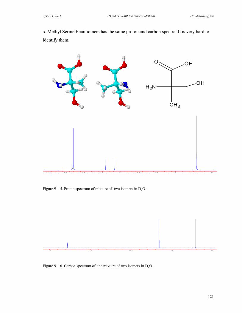
April 14, 2011 1Dand 2D NMR Experiment Methods Dr. Shaoxiong Wu
121
-Methyl Serine Enantiomers has the same proton and carbon spectra. It is very hard to
identify them.
CH3
NH2OH
O OH
Figure 9 – 5. Proton spectrum of mixture of two isomers in D2O.
Figure 9 – 6. Carbon spectrum of the mixture of two isomers in D2O.
5 . 5 5 . 0 4 . 5 4 . 0 3 . 5 3 . 0 2 . 5 2 . 0 1 . 5 P P M
2 0 0 1 5 0 1 0 0 5 0 P P M

April 14, 2011 1Dand 2D NMR Experiment Methods Dr. Shaoxiong Wu
122
Figure 9 – 7. Add 0.03 ml of Pr(hfc)3, the CH3 peak start to separate. By adding the Pure isomer solution into the above sample, the right peak increases the intensity. It suggested that the configuration of the pure sample is same as the upfield peak, on the right. From the reference, the right peak has the same configuration of the Pr(hfc)3, i.e. (R) ---isomer. And left peak is the S-isomer.
Conclusion: The pure compound is R-isomer, it corresponds the upfield shift with Pr(hfc)3. The mixture of S and R could be identified by Pr(hfc)3 at very low concentration in Methanol solvent. It is possible to calculate the relative amount of S and R in the mixture by titration of the pure sample.
5 . 0 4 . 5 4 . 0 3 . 5 3 . 0 2 . 5 2 . 0 1 . 5 P P M
1.46 1.44 1.42 1.40 1.38 1.36 1.34 PPM 1.46 1.44 1.42 1.40 1.38 1.36 1.34 PP 1.46 1.44 1.42 1.40 1.38 1.36 1.34 PP

April 14, 2011 1Dand 2D NMR Experiment Methods Dr. Shaoxiong Wu
123
D. Chemical Shift and Isotope Effects Isotopes have different mass such as 1H and 2H, although they have the same electronic environment, they have different vibrational levels. The chemical shifts of carbon that bound to 1H will be different from that when it bounds to 2H, since C-2H has a shorter bond length. Isotope effects are important because the method of substitution id widely used in practice. Selectively labeled compounds are used for the simplification of NMR spectra, or removal of degeneracy in the spectra. There are numerous applications of the study of isotope effects. More detailed information and application: Isotope effects in NMR spectroscopy by P. Diehl, E. Fluck.
Figure 9 - 8. Carbon spectrum of CDCl3.
Figure 9 – 9. Carbon spectrum of CDCl3 mix with 30% CHCl3, without proton decoupling.
Figure 9 – 10. Carbon spectrum of CDCl3 mix with 30% CHCl3, with proton decoupling.
79 78 77 76 PPM
79 78 77 76 PPM
79.5 79.0 78.5 78.0 77.5 77.0 76.5 76.0 75.5 PPM

April 14, 2011 1Dand 2D NMR Experiment Methods Dr. Shaoxiong Wu
124
10. Solid State NMR Introduction In solution NMR, spectra consist of sharp peaks due to averaging of anisotropic NMR signals by rapid random tumbling. In solid state NMR, however, spectra consist of very broad peaks, since molecule random tumbling is limited. If we place a solid sample into a 5 mm NMR tube and then acquire a proton spectrum, you will have the spectrum as following:
Figure 11 - 1. Spectrum of Solid Crystal of Menthol.
Figure 11 - 2. Spectrum of Menthol adsorbed very small amount of CDCl3.
Figure 11- 3. Spectrum of Menthol in CDCl3. High resolution solid state NMR spectra could provide the same type of information that is available from corresponding solution NMR spectra, but a number of special techniques, probes and equipment are necessary. The presence of broad peaks on the other hand, provides much information on chemistry, structure and dynamics in the solid state. A huge variety of solid state NMR experiments are available for measurement of
1 5 1 0 5 0 P P M
1 5 1 0 5 0 P P M
1 5 1 0 5 0 P P M

April 14, 2011 1Dand 2D NMR Experiment Methods Dr. Shaoxiong Wu
125
internuclear distances, such as REDOR, DRAWS; deconvolution of quadrupolar influenced spectra, such as MQMAS and TRAPDOR; probing site symmetry and chemistry, etc. Solid state NMR is rapidly becoming an established method for studying structures of biological molecules since many of them neither crystalline or soluble in solution such as membrane proteins, certain large enzymes and forms of amyloid. Thus, solid state NMR techniques often are complementary to other methods. Solid state NMR has been applied to the following fields, and its applications are still expending: organic and inorganic complexes, zeolites, microporous solids, biological molecules, cements, wood, food products, metal and alloys, polymers, archaelogical specimens, glasses etc. Most of the NMR active nuclei in the periodic table are available for investigation by solid state NMR.
Figure 11 - 4. Proton spectrum of Tuna Fish by using 4 mm HRMAS probe, spin at 4600 Hz.
Figure 11 – 5. CPMAS/TOSS 13C spectrum of a polymer membrane. 4 mm HXY probe spin at 6000 Hz.
14 12 10 8 6 4 2 0 -2 PPM
200 150 100 50 PPM
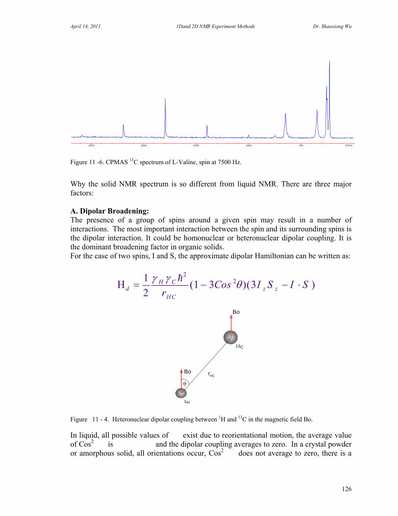
April 14, 2011 1Dand 2D NMR Experiment Methods Dr. Shaoxiong Wu
126
Figure 11 -6. CPMAS 13C spectrum of L-Valine, spin at 7500 Hz.
Why the solid NMR spectrum is so different from liquid NMR. There are three major factors: A. Dipolar Broadening: The presence of a group of spins around a given spin may result in a number of interactions. The most important interaction between the spin and its surrounding spins is the dipolar interaction. It could be homonuclear or heteronuclear dipolar coupling. It is the dominant broadening factor in organic solids. For the case of two spins, I and S, the approximate dipolar Hamiltonian can be written as:
dH C
HCz zr
Cos I S I S 1
21 3 3
22
( )( )
Figure 11 - 4. Heteronuclear dipolar coupling between 1H and 13C in the magnetic field Bo. In liquid, all possible values of ��exist due to reorientational motion, the average value of Cos2 ��is�������and the dipolar coupling averages to zero. In a crystal powder or amorphous solid, all orientations occur, Cos2 ��does not average to zero, there is a
250 200 150 100 50 PPM
1H
13C
rHCBo
Bo
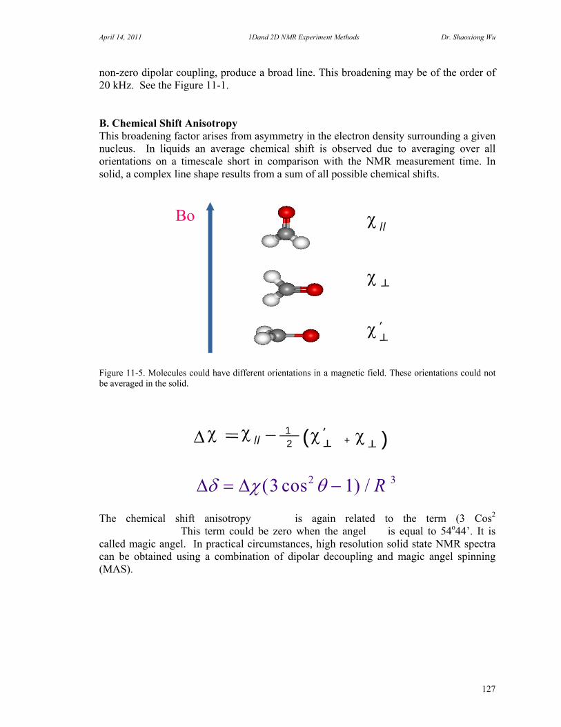
April 14, 2011 1Dand 2D NMR Experiment Methods Dr. Shaoxiong Wu
127
non-zero dipolar coupling, produce a broad line. This broadening may be of the order of 20 kHz. See the Figure 11-1.
B. Chemical Shift Anisotropy This broadening factor arises from asymmetry in the electron density surrounding a given nucleus. In liquids an average chemical shift is observed due to averaging over all orientations on a timescale short in comparison with the NMR measurement time. In solid, a complex line shape results from a sum of all possible chemical shifts.
Figure 11-5. Molecules could have different orientations in a magnetic field. These orientations could not be averaged in the solid.
The chemical shift anisotropy ����is again related to the term (3 Cos2 ��������� This term could be zero when the angel ��is equal to 54o44’. It is called magic angel. In practical circumstances, high resolution solid state NMR spectra can be obtained using a combination of dipolar decoupling and magic angel spinning (MAS).
12 ( + )
Bo
( cos ) /3 12 3R
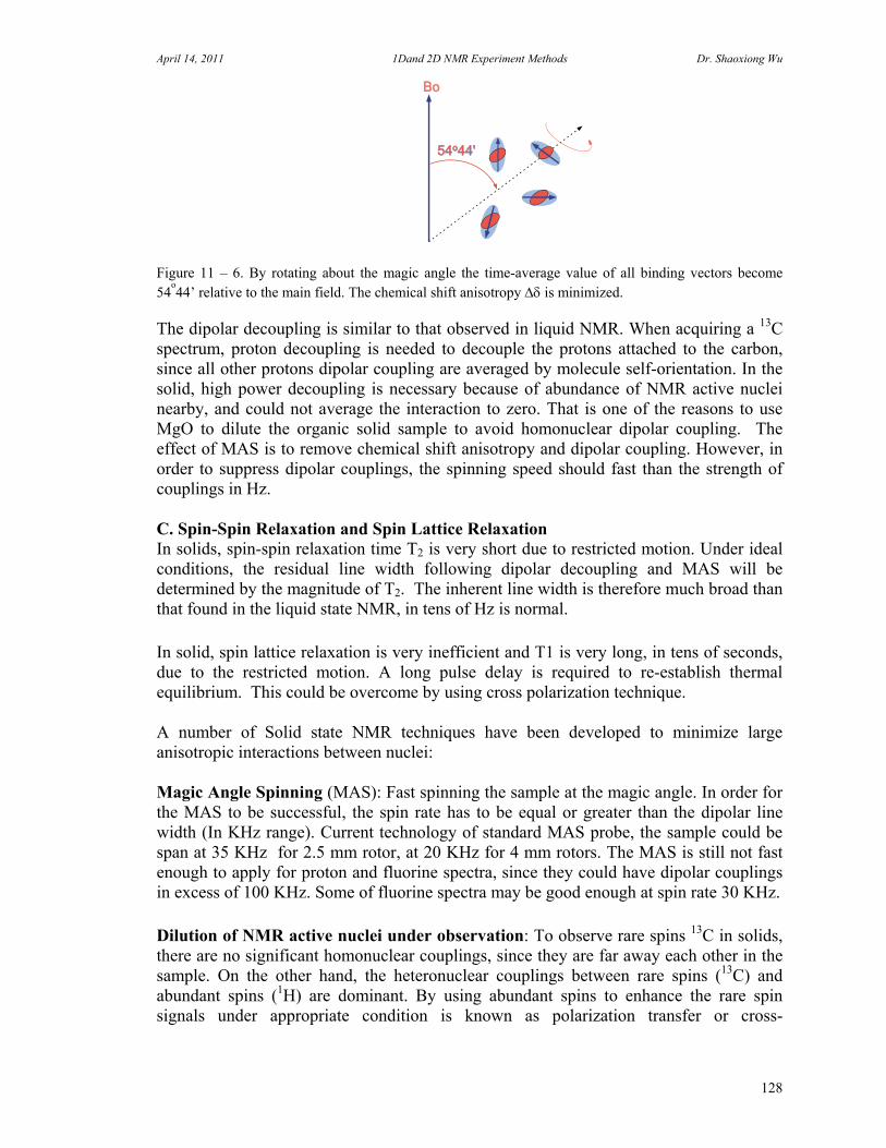
April 14, 2011 1Dand 2D NMR Experiment Methods Dr. Shaoxiong Wu
128
Figure 11 – 6. By rotating about the magic angle the time-average value of all binding vectors become 54
o44’ relative to the main field. The chemical shift anisotropy is minimized.
The dipolar decoupling is similar to that observed in liquid NMR. When acquiring a 13C spectrum, proton decoupling is needed to decouple the protons attached to the carbon, since all other protons dipolar coupling are averaged by molecule self-orientation. In the solid, high power decoupling is necessary because of abundance of NMR active nuclei nearby, and could not average the interaction to zero. That is one of the reasons to use MgO to dilute the organic solid sample to avoid homonuclear dipolar coupling. The effect of MAS is to remove chemical shift anisotropy and dipolar coupling. However, in order to suppress dipolar couplings, the spinning speed should fast than the strength of couplings in Hz. C. Spin-Spin Relaxation and Spin Lattice Relaxation In solids, spin-spin relaxation time T2 is very short due to restricted motion. Under ideal conditions, the residual line width following dipolar decoupling and MAS will be determined by the magnitude of T2. The inherent line width is therefore much broad than that found in the liquid state NMR, in tens of Hz is normal. In solid, spin lattice relaxation is very inefficient and T1 is very long, in tens of seconds, due to the restricted motion. A long pulse delay is required to re-establish thermal equilibrium. This could be overcome by using cross polarization technique. A number of Solid state NMR techniques have been developed to minimize large anisotropic interactions between nuclei: Magic Angle Spinning (MAS): Fast spinning the sample at the magic angle. In order for the MAS to be successful, the spin rate has to be equal or greater than the dipolar line width (In KHz range). Current technology of standard MAS probe, the sample could be span at 35 KHz for 2.5 mm rotor, at 20 KHz for 4 mm rotors. The MAS is still not fast enough to apply for proton and fluorine spectra, since they could have dipolar couplings in excess of 100 KHz. Some of fluorine spectra may be good enough at spin rate 30 KHz. Dilution of NMR active nuclei under observation: To observe rare spins 13C in solids, there are no significant homonuclear couplings, since they are far away each other in the sample. On the other hand, the heteronuclear couplings between rare spins (13C) and abundant spins (1H) are dominant. By using abundant spins to enhance the rare spin signals under appropriate condition is known as polarization transfer or cross-
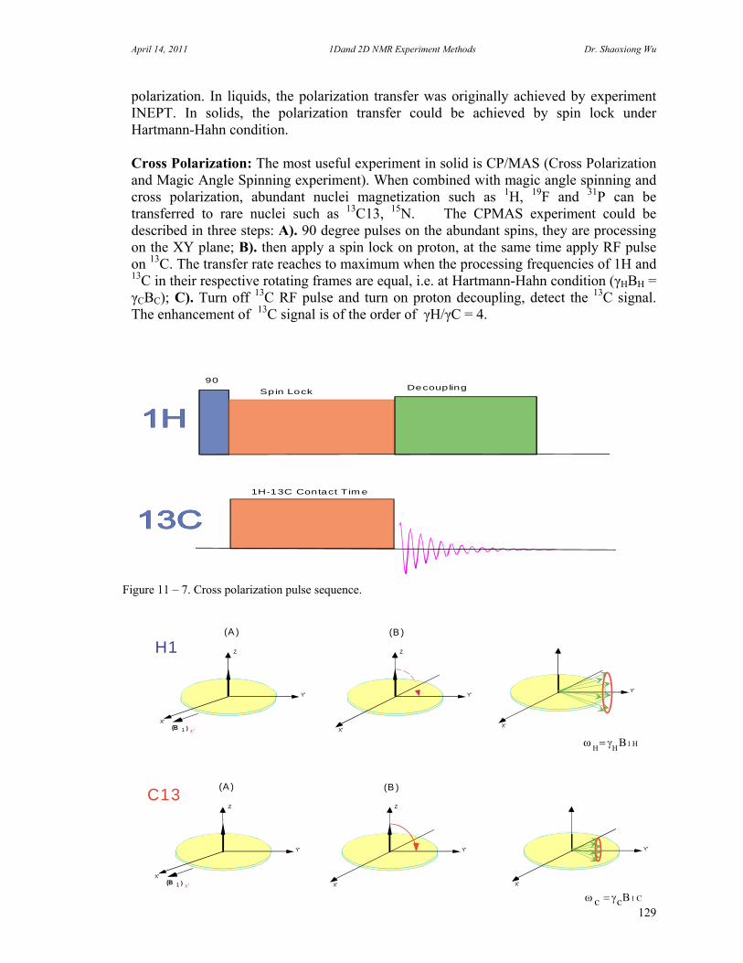
April 14, 2011 1Dand 2D NMR Experiment Methods Dr. Shaoxiong Wu
129
polarization. In liquids, the polarization transfer was originally achieved by experiment INEPT. In solids, the polarization transfer could be achieved by spin lock under Hartmann-Hahn condition. Cross Polarization: The most useful experiment in solid is CP/MAS (Cross Polarization and Magic Angle Spinning experiment). When combined with magic angle spinning and cross polarization, abundant nuclei magnetization such as 1H, 19F and 31P can be transferred to rare nuclei such as 13C13, 15N. The CPMAS experiment could be described in three steps: A). 90 degree pulses on the abundant spins, they are processing on the XY plane; B). then apply a spin lock on proton, at the same time apply RF pulse on 13C. The transfer rate reaches to maximum when the processing frequencies of 1H and 13C in their respective rotating frames are equal, i.e. at Hartmann-Hahn condition (γHBH = γCBC); C). Turn off 13C RF pulse and turn on proton decoupling, detect the 13C signal. The enhancement of 13C signal is of the order of γH/γC = 4.
Figure 11 – 7. Cross polarization pulse sequence.
X'
Y'
Z
(B 1 )
(A ) (B )
X'
Y'
Z
x '
X'
Y'
Z
(B 1 ) X'
Y'
(A ) (B )
Z
x ' X'
Y'
X'
Y'
H1
C13
c cC
90
Spin Lock Decoupling
1H-13C Contact Tim e

April 14, 2011 1Dand 2D NMR Experiment Methods Dr. Shaoxiong Wu
130
Figure 11 – 8. Cross polarization between 1H and 13C when the condition cH meet. Apply a 90 degree pulse on 1H. Then B1H shifts 90 degree on the X-Y plane and spin lock. Apply spin lock on the same axis as proton spin lock axis for 13C. The actual polarization takes place between proton and carbon during the contact time (in milliseconds). Then turn off the spin lock field on the 13C. Detect 13C signal and remain spin lock field for proton.
Figure 11- 9. CP/MAS 13C spectrum of Chitin. Solid State NMR Hardware For a dedicated solid state NMR, it should have following features:
a) Standard 89 mm bore size magnet. It allows most probes in variety applications such as HFX, HXY, HRMAS and Imaging Probes in different size to fit into the magnet.
250 200 150 100 50 0 PPM
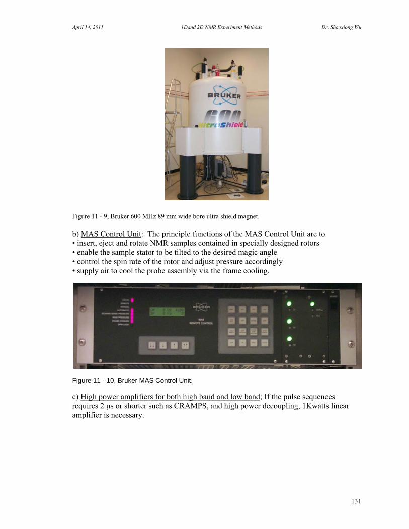
April 14, 2011 1Dand 2D NMR Experiment Methods Dr. Shaoxiong Wu
131
Figure 11 - 9, Bruker 600 MHz 89 mm wide bore ultra shield magnet. b) MAS Control Unit: The principle functions of the MAS Control Unit are to • insert, eject and rotate NMR samples contained in specially designed rotors • enable the sample stator to be tilted to the desired magic angle • control the spin rate of the rotor and adjust pressure accordingly • supply air to cool the probe assembly via the frame cooling.
Figure 11 - 10, Bruker MAS Control Unit. c) High power amplifiers for both high band and low band; If the pulse sequences requires 2 μs or shorter such as CRAMPS, and high power decoupling, 1Kwatts linear amplifier is necessary.

April 14, 2011 1Dand 2D NMR Experiment Methods Dr. Shaoxiong Wu
132
Figure 11 - 11, Front of Bruker BLAX1000 low band amplifier. d) Solid State NMR Probes: A solid state NMR probe is a very complex equipment that contains RF circuits, spin air and VT air supply, spin rate sensor, temperature sensor, tuning knobs etc in a very small space. There is one RF coil that allows to tune two to four different resonance frequencies. Also it requires the axis of RF coil is 54.44o relative to the main field.
Figure 11 - 12. Left: 4 mm turbine block and sample coil. Right: a HXY triple resonance probe is installed in the magnet. The connections include: three RF cables, two VT sensor, one cooling air, one bearing air, one driving air and one heater. All three channel tuning knobs and Magic angle adjust knob are under the probe. e) MAS Sample Rotor, Caps, Inserts and Sample Packing: In order for the rotor to spin stable and fast, the rotor has to be well packed and balanced. Load the sample evenly into the rotor barrel and tap the rotor lightly. Liquid or viscous samples are easily loaded using a small pipette. The rotor cap must be push into the rotor tightly. If the cap is improperly positioned, the rotor may not spin. Mark half of the beveled rim on the bottom of the rotor with a black marker for optical spin rate detection.
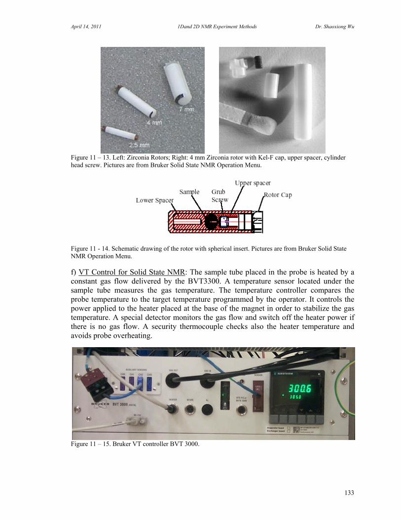
April 14, 2011 1Dand 2D NMR Experiment Methods Dr. Shaoxiong Wu
133
Figure 11 – 13. Left: Zirconia Rotors; Right: 4 mm Zirconia rotor with Kel-F cap, upper spacer, cylinder head screw. Pictures are from Bruker Solid State NMR Operation Menu.
Figure 11 - 14. Schematic drawing of the rotor with spherical insert. Pictures are from Bruker Solid State NMR Operation Menu.
f) VT Control for Solid State NMR: The sample tube placed in the probe is heated by a constant gas flow delivered by the BVT3300. A temperature sensor located under the sample tube measures the gas temperature. The temperature controller compares the probe temperature to the target temperature programmed by the operator. It controls the power applied to the heater placed at the base of the magnet in order to stabilize the gas temperature. A special detector monitors the gas flow and switch off the heater power if there is no gas flow. A security thermocouple checks also the heater temperature and avoids probe overheating.
Figure 11 – 15. Bruker VT controller BVT 3000.
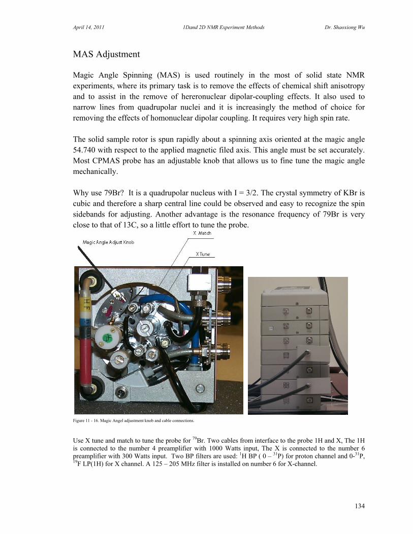
April 14, 2011 1Dand 2D NMR Experiment Methods Dr. Shaoxiong Wu
134
MAS Adjustment Magic Angle Spinning (MAS) is used routinely in the most of solid state NMR experiments, where its primary task is to remove the effects of chemical shift anisotropy and to assist in the remove of hereronuclear dipolar-coupling effects. It also used to narrow lines from quadrupolar nuclei and it is increasingly the method of choice for removing the effects of homonuclear dipolar coupling. It requires very high spin rate. The solid sample rotor is spun rapidly about a spinning axis oriented at the magic angle 54.740 with respect to the applied magnetic filed axis. This angle must be set accurately. Most CPMAS probe has an adjustable knob that allows us to fine tune the magic angle mechanically. Why use 79Br? It is a quadrupolar nucleus with I = 3/2. The crystal symmetry of KBr is cubic and therefore a sharp central line could be observed and easy to recognize the spin sidebands for adjusting. Another advantage is the resonance frequency of 79Br is very close to that of 13C, so a little effort to tune the probe.
Figure 11 - 16. Magic Angel adjustment knob and cable connections.
Use X tune and match to tune the probe for 79Br. Two cables from interface to the probe 1H and X, The 1H is connected to the number 4 preamplifier with 1000 Watts input, The X is connected to the number 6 preamplifier with 300 Watts input. Two BP filters are used: 1H BP ( 0 – 31P) for proton channel and 0-31P, 19F LP(1H) for X channel. A 125 – 205 MHz filter is installed on number 6 for X-channel.

April 14, 2011 1Dand 2D NMR Experiment Methods Dr. Shaoxiong Wu
135
Sample and Preparation: KBr (Potassium Bromide). Fill a 4mm ZrO2 solid state NMR rotor tightly and evenly with finely powered KBr. Use spin test station, make sure it is able to spin at 5 – 8KHz. Keep the sample in a dry box when it is not in use since KBr is very hygroscopic. Parameters: TD: 2k Pulprog: zg SW: 125k NS: 64 O1: on the resonance of KBr signal AQ: 8.2ms P1: 10us PL1: 20DB D1: 500ms RG: 256 Spin Rate: 5KHz SFO1: 150.365 MHz
Figure 11 - 17. a). FID of 79Br after the magic angle has been properly adjusted. B) 79Br spectrum after the magic angle has been properly adjusted.
0.001 0.002 0.003 0.004 0.005 0.006 0.007 sec
400 300 200 100 0 -100 -200 -300 PPM
April 14, 2011 1Dand 2D NMR Experiment Methods Dr. Shaoxiong Wu
136
Appendix A
There are two main ways to describe a spin system in the magnetic field: vector picture and density matrix. By
using the time dependent Schrödinger equation, we could treat a spin system in a magnetic field as a vector
according to the principle of mechanic theory. The advantage of this treatment is simple and easy to understand,
but many of the newer and now most of important NMR studies, especially solid state NMR, cannot be
understood by this treatment because it ignores quantum effects and in some cases, this will give different
answers. The density matrix treatment is a simple mathematical formalism that gives us the best of the quantum
and classical approaches. It preserves all classical and quantum features, the time dependent phenomena of a
spin system such as phase and coherence transfer can be understood. The disadvantage of this treatment is very
tedious and gives very little physical description of the manipulation of the spin system.
There are a large number of nuclei, such as 1H, 13C, and 31P, which have a nonzero spin angular momentum,
Ih/2π. According to the principle of quantum mechanics, I can take the values 1/2, 1, 3/2, etc. The
Hamiltonian corresponding to the spin quantum number I in a magnetic field:
20
hI A-1
where γ is the magnetogyric ratio, a characteristic of the nucleus and is either positive or negative and Bo is the
magnetic field chosen by convention to be the z axis of the laboratory coordinate. For a spin I, under the
influence of a magnetic field, the energy levels split into (2I + 1) sublevels. The energy difference between
neighboring levels can be expressed by:
20 ImhB
E A-2
where mI takes values ±I, ±(I - 1), ...., ±1/2 or 0 depending on whether I is a half-odd integer or an integer.
Zeeman energy levels are displaced by the constant value, γhBo/2π, which generally can be expressed in
frequency units and is called Larmor frequency of the isotope in the field Bo. This resonance frequency is
found to vary in direct proportion to the applied field, thus the larger the magnetic field the higher the resonance
frequency. In an ensemble of nuclear spins I, the (2I + 1) allowed energy levels are populated in thermal
equilibrium in accordance with the Boltzmann distribution. For a spin I= 1/2, the ratio of number spins in
higher state (β) and in lower state (α) is given by:
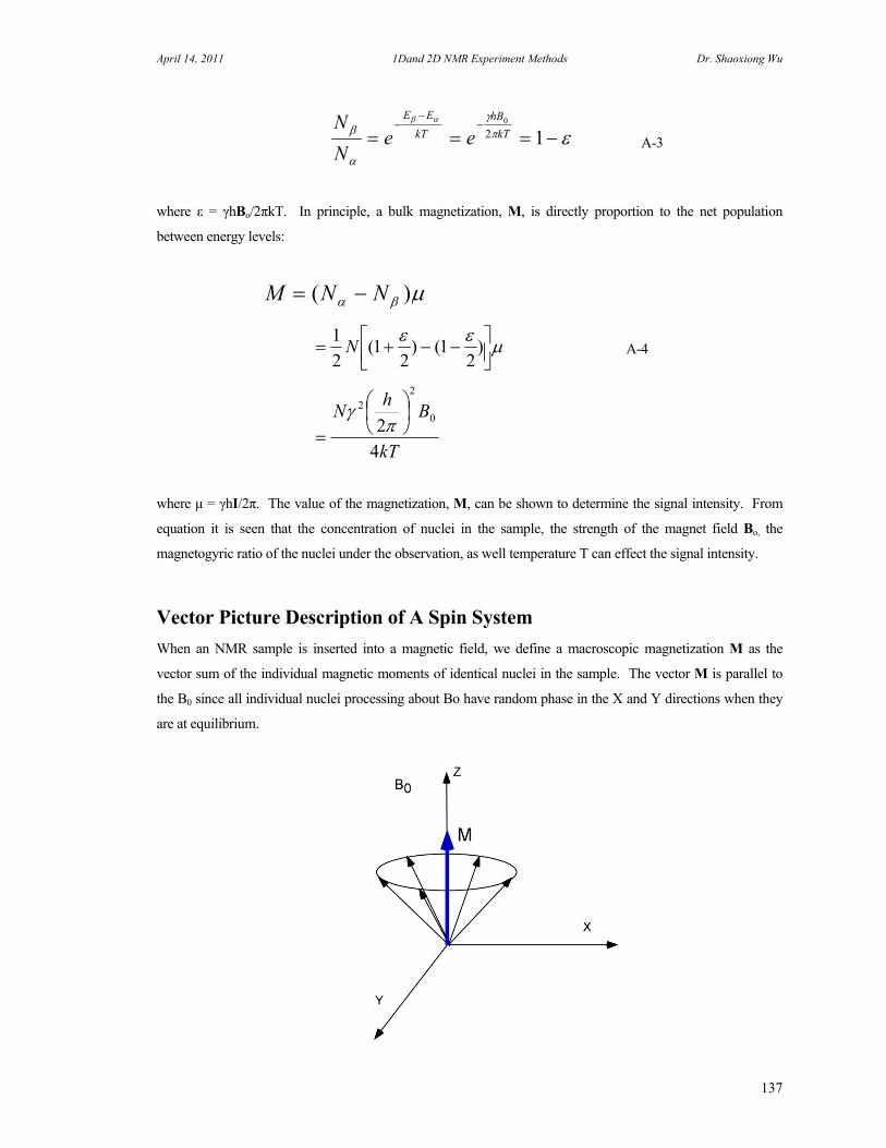
April 14, 2011 1Dand 2D NMR Experiment Methods Dr. Shaoxiong Wu
137
120
kT
hB
kT
EE
eeN
N A-3
where ε = γhBo/2πkT. In principle, a bulk magnetization, M, is directly proportion to the net population
between energy levels:
)( NNM
)
21()
21(
2
1N A-4
kT
Bh
N
42 0
22
where μ = γhI/2π. The value of the magnetization, M, can be shown to determine the signal intensity. From
equation it is seen that the concentration of nuclei in the sample, the strength of the magnet field Bo, the
magnetogyric ratio of the nuclei under the observation, as well temperature T can effect the signal intensity.
Vector Picture Description of A Spin System
When an NMR sample is inserted into a magnetic field, we define a macroscopic magnetization M as the
vector sum of the individual magnetic moments of identical nuclei in the sample. The vector M is parallel to
the B0 since all individual nuclei processing about Bo have random phase in the X and Y directions when they
are at equilibrium.

April 14, 2011 1Dand 2D NMR Experiment Methods Dr. Shaoxiong Wu
138
Figure A-1. Vector M represents an ensemble of identical nuclei that process along Z at random phase in the
magnetic field B0.
For an NMR experiment, the M is manipulated by RF pulses, then a free induction decay (FID) of the M is
detected. A pulse sequence could be described by using vectors. See previous chapters.
Note:
Wavefunctions (Ψ, φ)
A state of a spin system in specified environment could be described by a Wavefunction. It is a mathematical
function by witch we could determine the value of the physical observables.
Operators, expectation Values (Ô, <A>)
An operator is something witch acts on a function to produce another function. The expectation value of the
corresponding operator is a physical observable in a state described by the wavefunction, Ψ.
d
dA
*
* ˆ
Schrodinger Equation, Hamiltonian, Eigenfunction and Eigenvalue
The time independent Schrodinger equation:
ˆˆ
The time dependent Schrodinger equation:
ti t
tt
)(
)()(ˆ
Spin Operator and Spin State
To determine spin properties of a nucleus, we operate on the nuclear spin wavefunction with a spin operator.
________________________________________________________________________
Density Matrix Description of a Spin System
According to the principle of quantum mechanics, a spin system consisting of N nuclei, each of spin (if I = ½)
there are 2N spin state functions i.e. φ1, φ2 for N=1, and φ1, φ2, φ3, and φ4 for N=2, etc. As well as there are
2N wavefunctions that describing the state of all nuclear spins, i.e. ψ1, ψ2 for N=1 and ψ1, ψ2, ψ3 and ψ4 for N

April 14, 2011 1Dand 2D NMR Experiment Methods Dr. Shaoxiong Wu
139
= 2, etc. These wavefunctions can always be described as a linear combination of these spin state functions φ1,
φ2 etc. That become a complete set of basis functions and it is specified by:
N
kkk
i C2
1
A-5
If I = ½ and only one spin, N=1, there will be two basis functions as a complete set:
2121
11
1 CC 2221
21
2 CC A-6
or
111
1 C ; if 12C = 0 and 11
1 C
222
2 C ; if 21C = 0 and 12
2 C
where φi are spin state functions or the eigenstates of the Zeeman Hamiltonian since one spin and I= ½, there
are two possible energy levels, in convention, we write them as -½ and ½, or α and β state. From basic
quantum theory, the value of an observable quantity A that could be represented by a operator Â, can be found
for any state i as the expectation value, <A>i.
)()( iiiAA
N
jiji
ij
ii ACC
2
1,
*)()(*
N
jiij
ij
ii ACC
2
1,
)()(* A-7
Now we consider an ensemble of spins in which each of 2N states has a certain probability of occurring, Pi. We
can describe as average over the ensemble by:
N
i
iiP2
1
A-8
or if I =1/2 and only one spin
22
211
1 CPCP
where P(i) are the probabilities of the states occurring in an ensemble.
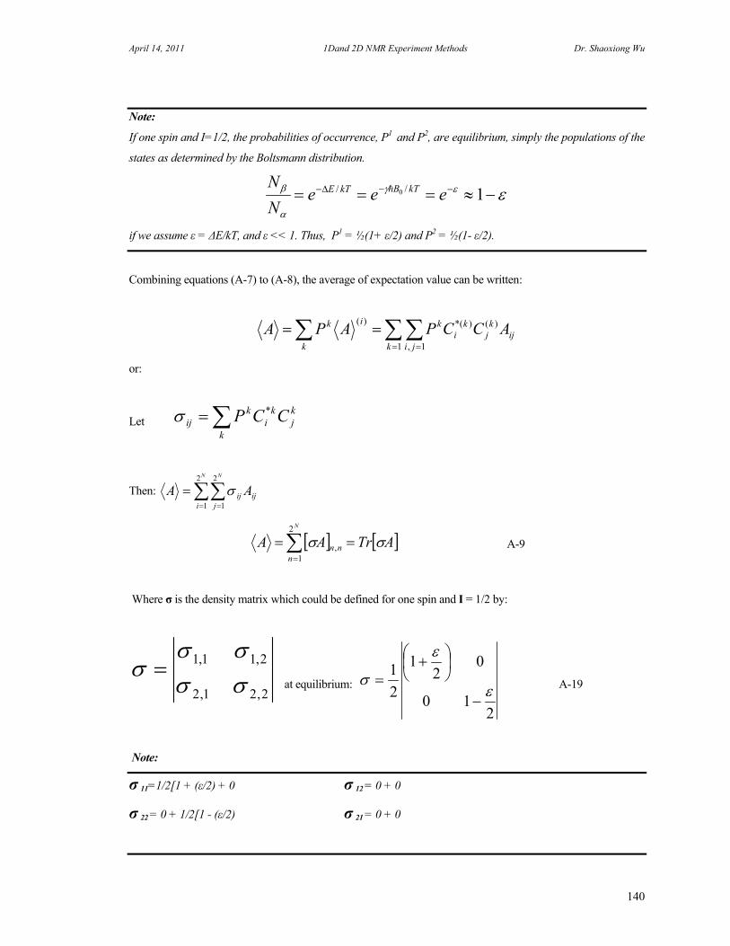
April 14, 2011 1Dand 2D NMR Experiment Methods Dr. Shaoxiong Wu
140
Note:
If one spin and I=1/2, the probabilities of occurrence, P1 and P2, are equilibrium, simply the populations of the
states as determined by the Boltsmann distribution.
1// 0 eeeN
N kTBkTE
if we assume ε = ΔE/kT, and ε << 1. Thus, P1 = ½(1+ ε/2) and P2 = ½(1- ε/2).
Combining equations (A-7) to (A-8), the average of expectation value can be written:
1 1,
)()*()(
k jiij
kj
ki
ki
k
k ACCPAPA
or:
Let k
kj
ki
kij CCP *
Then:
N N
i jijij AA
2
1
2
1
ATrAAN
nnn
2
1, A-9
Where σ is the density matrix which could be defined for one spin and I = 1/2 by:
2,21,2
2,11,1
at equilibrium:
210
02
1
2
1
A-19
Note:
σ 11=1/2[1 + (ε/2) + 0 σ 12 = 0 + 0
σ 22 = 0 + 1/2[1 - (ε/2) σ 21 = 0 + 0
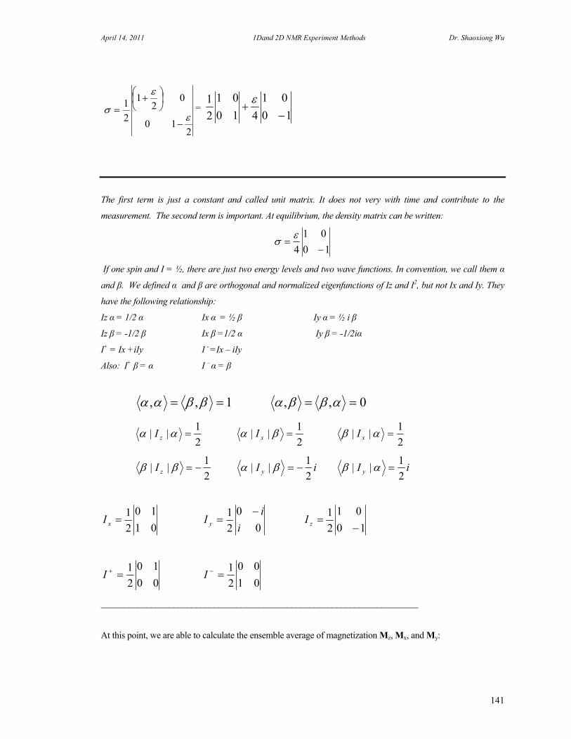
April 14, 2011 1Dand 2D NMR Experiment Methods Dr. Shaoxiong Wu
141
210
02
1
2
1
= 10
01
410
01
2
1
The first term is just a constant and called unit matrix. It does not very with time and contribute to the
measurement. The second term is important. At equilibrium, the density matrix can be written:
10
01
4
If one spin and I = ½, there are just two energy levels and two wave functions. In convention, we call them α
and β. We defined α and β are orthogonal and normalized eigenfunctions of Iz and I2, but not Ix and Iy. They
have the following relationship:
Iz α = 1/2 α Ix α = ½ β Iy α = ½ i β
Iz β = -1/2 β Ix β =1/2 α Iy β = -1/2iα
I+ = Ix +iIy I - =Ix – iIy
Also: I+ β = α I – α = β
1,, 0,,
2
1|| zI
2
1|| xI
2
1|| xI
2
1|| zI iI y 2
1|| iI y 2
1||
01
10
2
1xI
0
0
2
1
i
iI y
10
01
2
1
zI
00
10
2
1I
01
00
2
1I
______________________________________________________________________
At this point, we are able to calculate the ensemble average of magnetization Mz, Mx, and My:

April 14, 2011 1Dand 2D NMR Experiment Methods Dr. Shaoxiong Wu
142
)( zz MTrM
= )(2
zITrhN
=
10
01
2
1
210
02
1
2
1
2
TrhN
=kT
BNhN
4420
22
A-11
)(2 xx ITr
hNM
A-12
= 001
10
2
1
210
02
1
2
1
2
TrhN
)(2 yy ITr
hNM
A-13
= 001
10
2
1
210
02
1
2
1
2
TrhN
where Ix, Iy, Iz are the spin operators corresponding to Mx, My, Mz. These results are same as calculated from
classic model and confirm that there is no transverse magnetization when in thermal equilibrium. If a
perturbation pulse supplied to the system, which can be presented by a group of operators applying on the spin
system. We now have a formula for constructing the density matrix for any spin system in terms of a set of
basis functions, we are also can determine the expectation value. However, we still need an expression for time
dependent processes.
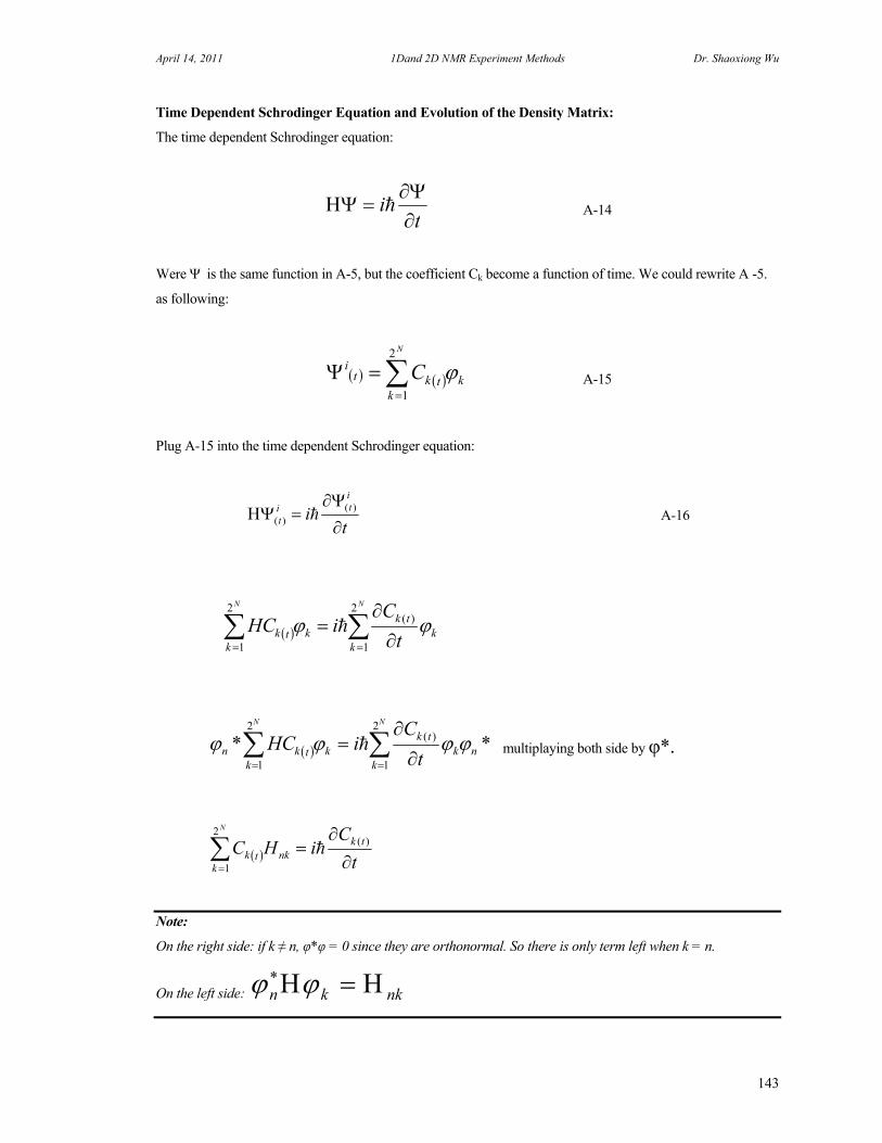
April 14, 2011 1Dand 2D NMR Experiment Methods Dr. Shaoxiong Wu
143
Time Dependent Schrodinger Equation and Evolution of the Density Matrix:
The time dependent Schrodinger equation:
ti
A-14
Were Ψ is the same function in A-5, but the coefficient Ck become a function of time. We could rewrite A -5.
as following:
N
kktkt
i C2
1
A-15
Plug A-15 into the time dependent Schrodinger equation:
ti
iti
t
)()( A-16
NN
kk
tk
kktk t
CiHC
2
1
)(2
1
**2
1
)(2
1n
kk
tk
kktkn
NN
t
CiHC
multiplaying both side by φ*.
t
CiHC tk
nkk
tk
N
)(2
1
Note:
On the right side: if k ≠ n, φ*φ = 0 since they are orthonormal. So there is only term left when k = n.
On the left side: nkkn

April 14, 2011 1Dand 2D NMR Experiment Methods Dr. Shaoxiong Wu
144
In order to get a time dependence of density matrix, we could use the equation A-9.
k
kj
ki
kij CCP *
or
kji
kij CCP
tt*
k
ijikkjij
i
ijij
i
_________________________________________________________________________
Note:
j
iji
ji Ct
C
t
CC
t
CC
Use equation A- 16
j
kjkk
kkjki CC
iCC
i
)( k
jkikkjji CCCCi
For more general form:
i
t
or it could integrated to give:
/)0(
/)(
titit ee
This is the Liouville-von Neumann equation. It is the time dependent Schrodinger equation for an ensemble of
spins. The density matrix describing the ensemble will evolve in time if the density operators do not commute
with Hamiltonian.
Note:
If two operators commute, they have identical eigenfunctions and the commutator of them is defined as:

April 14, 2011 1Dand 2D NMR Experiment Methods Dr. Shaoxiong Wu
145
ABBABA ˆˆˆˆˆ,ˆ
_________________________________________________________________________
Using this result we may calculate σ for the pulse sequence. For example, a pulse sequence 90-τ-180-τ-acq,
used for measuring molecular self-diffusion coefficients, is presented in Figure A-1. The spin system is
perturbed by two pulses, there are associated with these pulses density matrixes which is presented in the
equation. Where I's are the operators corresponding to the pulses, and C's are the constants related to the
chemical shifts and delay time τ. From these density matrixes, the evolution in terms of propagator can be
calculated and the observed spectra features including intensity, frequency, phase, and multiplet structure can
be notified.

April 14, 2011 1Dand 2D NMR Experiment Methods Dr. Shaoxiong Wu
146
Appendix B I believe you will find this list of acronym useful in your studying NMR techniques, as well as their applications.
Acronym Definition and Description
APT Attached Proton Test
ADC Analog-to-Digital Converter
BIRD Bilinear Rotation Decoupling
CAMELSPIN Cross-Relaxation Appropriate for Minimolecules Emulated by locked Spins
CIDNP-NMR Chemically-Induced Dynamic Nuclear Polarization-NMR
COLOC Correlation Spectroscopy for long –Range Coupling
COSY Correlated Spectroscopy
CPD Composite Pulse Decoupling
CPMAS Cross Polarization Magic Angle Spining
CPMG Carr-Purcell-Meiboom-Gill Sequence
CRAMPS Combined Rotation and Multiple-Pulse Spectroscopy
DANTE Delays Alternating with Nutations for Tailored Excitation
DEPT Distortionless Enhancement by Polarization Transfer
DOSY Diffusion-Ordered Spectroscopy
DQC Double Quantum Coherence
DQF-COSY Double Quantum Filter COSY
DRAWS Dipolar Recoupling with A Windownless Sequence
EXSY Exchange Spectroscopy
GARP Globally Optimized Alternating phase Rectangular Pulses
GE Gradient Enhanced spectroscopy
HETCOR Heteronuclear Correlation
HETLOC Long Range HETCOR
HMQC Heteronuclear Multiple Quantum Correlation
HMBC Heteronuclear Multiple Bond Correlation
HOSY Heteronuclear Overhauser Enhancement Spectroscopy
HOHAHA Homonuclear Hartmann Hahn Spectroscopy
HSQC Heteronuclear Single QuantumCoherence
INADEQUATE Incredible Nattural Abundance DoublE QUAntum Transfer Experiment
INEPT Insensitive Nucleus Enhancement by Polarization Transfer
LC-NMR Liquid Chromatography-NMR
LG Lorentz-Gauss
MLEV Composite Pulse decoupling sequence
MQF Multiple Quantum Filter
NOE Nuclear Overhauser Effect
NOESY Nuclear Overhauser and Exchange Spectroscopy

April 14, 2011 1Dand 2D NMR Experiment Methods Dr. Shaoxiong Wu
147
PFG Pulsed Field Gradient
REDOR Rotational Echo DOuble Resonance
RELAY Relayed Correlation Spectroscopy
ROESY Rotating Frame Overhauser Enhancement Spectroscopy
SECSY Spin Echo Correlated Scpectroscopy
TEDOR Transferred Echo Double Resonance
TOCSY Total Correlation Spectroscopy
TOSS Total Suppression od Sidebands
TPPI Time Proportional Phase Incrementation
WALTZ Wideband Alternating Phase Low power technique for zero residual splitting
WATERGATE Water Suppression by Gradient-Tailored Excitation
WEFT Water-Eliminated Fourier Transform
Z-COSY z-filtered COSY
ZQC Zero quantum Coherence