shape design from exemplar sketches using …vdel.me.cmu.edu/publications/2012jmd/paper.pdf ·...

Gunay Orbay

Levent Burak Kara1

e-mail: [email protected]

Department of Mechanical Engineering,Carnegie Mellon University,

Pittsburgh, PA 15213

Shape Design From ExemplarSketches Using Graph-BasedSketch AnalysisWe describe a new technique that works from a set of concept sketches to support the ex-ploration and engineering of products. Our approach allows the capture and reuse ofgeometric shape information contained in concept sketches, as a means to generate solu-tions that can concurrently satisfy aesthetic and functional requirements. At the heart ofour approach is a graph-based representation of sketches that allows the determinationof topological and geometric similarities in the input sketches. This analysis, when com-bined with a geometric deformation analysis, results in a design space from which newshapes can be synthesized, or a developing design can be optimized to satisfy prescribedobjectives. Moreover, it facilitates a sketch-based, interactive editing of existing designsthat preserves the shape characteristics captured in the design space. A key advantage ofthe proposed method is that shape features common to all sketches as well as thoseunique to each sketch can be separately identified, thus allowing a mixing of differentsketches to generate a topologically and geometrically rich set of conceptual alternatives.We demonstrate our technique with 2D and 3D examples. [DOI: 10.1115/1.4007147]

1 Introduction

Early design activities frequently involve the generation of awide variety of concepts [1]. Designers commonly record suchideas in the form of conceptual sketches, which are recognized tobe critically important for product design and development [2–5].These sketches help designers assess different concepts and gener-ate new ones early on, but rarely get utilized in the digital phasesof the design process. This is mainly because current software isseverely limited when such informal representations are con-cerned. In product form design specifically, while conceptsketches embody a rich set of geometric information regarding theshape of the design, most of this information merely serves asstatic visual references, rather than providing a means to expeditethe development and engineering of the product.

Furthermore, product form design is heavily affected by down-stream engineering considerations, as the final product is requiredto satisfy both aesthetic and functional requirements. Typically,candidate designs generated by the styling teams have to be eval-uated and validated by the engineering teams. This necessitates aniterative process involving multiple parties, which can signifi-cantly impact the design cost and duration. As a result, only ahandful of concepts may be adequately developed, while manyare prematurely eliminated.

In this work, we attempt to enhance the passive usage of con-ceptual sketches. We propose a new method that converts the geo-metric information stored in the sketches into a computationallysuitable form. The proposed method does so by automaticallyidentifying emerging shape ideas from the commonly appearingpatterns, and concept specific design features. These patterns andfeatures serve as means to computationally encode the shape ideascontained in the sketches to construct a design space. This designspace allows (1) synthesis of novel forms through nonlinear mix-ing of input sketches, (2) a style-preserving free-form explorationof the design space through interactive sketching, and (3) produc-tion of design solutions that satisfy prescribed engineering objec-tives and constraints.

2 Related Work

We group the previous studies on computational conceptualdesign systems in three categories. We give a summary ofexample-based design approaches and related difficulties in prac-tical applications. We then discuss generative design methods andassociated challenges. Finally, we review the major sketch-baseddesign systems that support conceptual design and geometricmodeling.

2.1 Example-Based Design Methods. Example-based designmethods are primarily based on geometric shape interpolationtechniques [6,7]. The first application to industrial design was pro-posed by Chen and Parent in 1989 [8]. Wang [9] extended theidea and combined shape interpolation with geometric transforma-tion. Hsiao and Liu proposed using similar techniques for Com-puter Aided Design (CAD) models [10] or for scan-digitizedgeometries [11]. Similarly, Chen et al. [12] used image interpola-tion to study the mapping between car shapes and their descriptivecharacteristics. Kang and Lee [13] used mesh-based interpolationon different 3D ship hull forms to generate new forms.

The majority of these techniques require input models to begeometrically preregistered to resolve the mapping problem.Hence, an automatic identification of such correspondences hasalso been a popular research topic [7]. Despite these advances, thestrict correspondence requirement limits example-based designapproaches to mainly topologically equivalent geometries. More-over, most approaches work from existing models, or require signif-icant effort for model creation. In conceptual design, these methodshave found limited usage as the content at these stages is incom-plete, exploratory, and may exhibit large intermodel variations. Ourwork, on the other hand, is designed to work on geometrically andtopologically different conceptual sketches. A key advance is agraph-based representation that enables the identification of a formcommon to all sketches, as well as features unique to each sketch.

2.2 Generative Design Methods. Generative methods focuson determining a parametrization and a set of generative rules fora product, using a set of existing designs. New designs can be syn-thesized from these learned rules. Cagan and Agarwal proposedusing shape grammars as a language for defining template topolo-gies through geometric rules [14]. McCormack et al. used thisapproach to study brand identity [15]. Orsborn et al. proposed

1Corresponding author.Contributed by the Design Theory and Methodology Committee of ASME for

publication in the JOURNAL OF MECHANICAL DESIGN. Manuscript received May 27,2011; final manuscript received July 1, 2012; published online October 2, 2012.Assoc. Editor: Karthik Ramani.

Journal of Mechanical Design NOVEMBER 2012, Vol. 134 / 111002-1Copyright VC 2012 by ASME

Downloaded From: http://mechanicaldesign.asmedigitalcollection.asme.org/ on 02/26/2015 Terms of Use: http://asme.org/terms

combining different vehicle classes using shape grammars [16].Although useful as a generative language, current shape grammartechniques require the rules to be determined and defined man-ually. In this work, we aim to circumvent rule specification usingan automatic geometric deformation analysis, which lends itself toa generative design process.

Among the class of generative methods, genetic algorithms(GA) have been a popular choice for design [17–21]. Smyth andWallace used GAs to synthesize aesthetic forms through manual vis-ual inspection [17]. Frazer et al. utilized GAs to synthesize envelopedesigns for sky scrapers [18]. Bezirtzis et al. extended these applica-tions to 3D models [19]. Wannarumon et al. used similar techniquestogether with prescribed aesthetic metrics for jewelry design [20].Although GAs are successful in generating novel product forms, theyrequire the model parametrization to be specified a priori. Moreover,parameter quality dictates the variety of designs that can be gener-ated. This parameterization typically requires manual intervention.

2.3 Sketch-Based Design Systems. Recent years have seenthe development of many sketch-based computer interfaces forCAD modeling. New methods allow the creation of curves andsurfaces via intuitive free-hand sketching. Earlier studies werefocused on creating primitive geometries [22,23] using sketchinput. Recent studies [24–28] attempt to enable free-form surfacecreation from simple strokes and gestures. One group [24–26]focuses on creating initial blobs on which more features can beadded while producing smooth surfaces. Another group [27,28]suggests creating curves in 3D which are later utilized as con-struction curves for free-form surfaces. A comprehensive analysisof existing work on sketch-based modeling can be found in Ref.[29]. These sketch-based methods primarily focus on using thesketch input for geometry creation rather than using the shapeideas in the geometries to generate new design concepts.

The above approaches aim to support product design by gener-ating design alternatives, by learning design preferences from ex-perience, and by creating 3D geometries from sketch input.However, these studies provide little or no means to learning theshape ideas contained in the conceptual design sketches and usingthem to aid the design process. In this work, we aim to providesupport for shape design using explicitly encoded geometric infor-mation extracted from conceptual design sketches. In contrast toprior work, our approach is designed to be useful in the earlydesign stages where concepts are articulated in the form of simplesketches. This allows working from a set of designs by automati-cally identifying a common form and concept specific design fea-tures, which then serve as a design space.

3 Method Overview and User Input

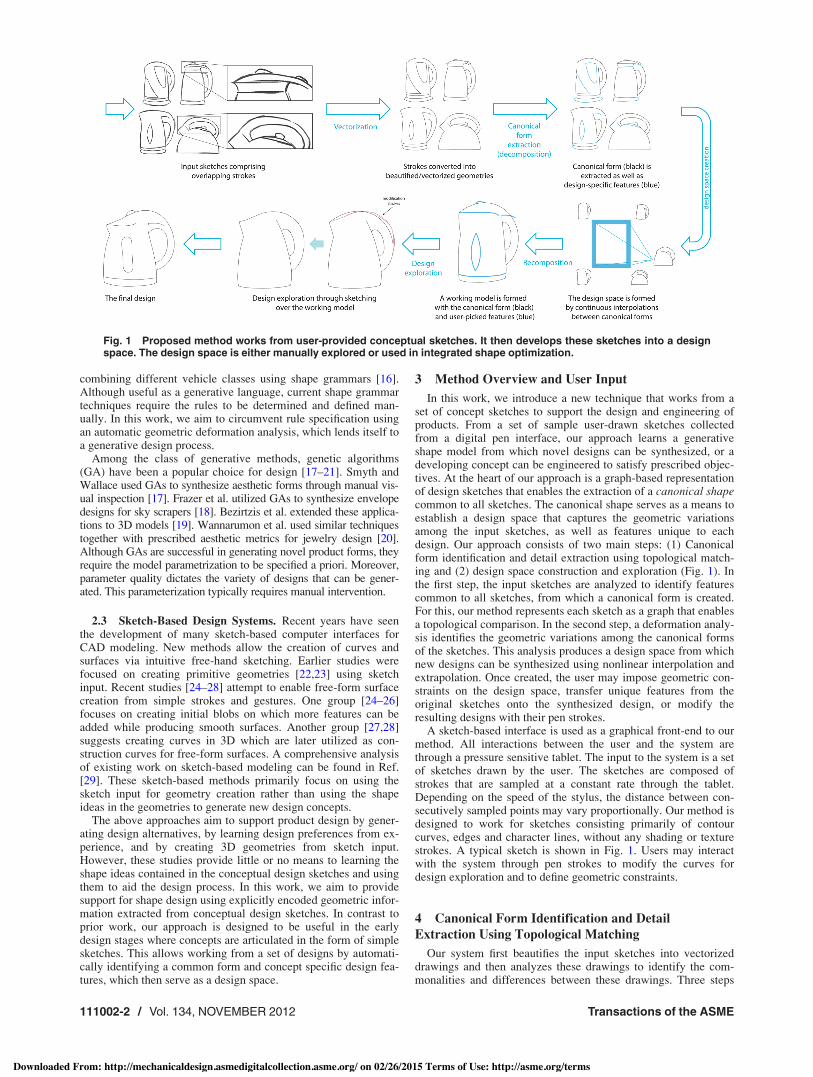
In this work, we introduce a new technique that works from aset of concept sketches to support the design and engineering ofproducts. From a set of sample user-drawn sketches collectedfrom a digital pen interface, our approach learns a generativeshape model from which novel designs can be synthesized, or adeveloping concept can be engineered to satisfy prescribed objec-tives. At the heart of our approach is a graph-based representationof design sketches that enables the extraction of a canonical shapecommon to all sketches. The canonical shape serves as a means toestablish a design space that captures the geometric variationsamong the input sketches, as well as features unique to eachdesign. Our approach consists of two main steps: (1) Canonicalform identification and detail extraction using topological match-ing and (2) design space construction and exploration (Fig. 1). Inthe first step, the input sketches are analyzed to identify featurescommon to all sketches, from which a canonical form is created.For this, our method represents each sketch as a graph that enablesa topological comparison. In the second step, a deformation analy-sis identifies the geometric variations among the canonical formsof the sketches. This analysis produces a design space from whichnew designs can be synthesized using nonlinear interpolation andextrapolation. Once created, the user may impose geometric con-straints on the design space, transfer unique features from theoriginal sketches onto the synthesized design, or modify theresulting designs with their pen strokes.

A sketch-based interface is used as a graphical front-end to ourmethod. All interactions between the user and the system arethrough a pressure sensitive tablet. The input to the system is a setof sketches drawn by the user. The sketches are composed ofstrokes that are sampled at a constant rate through the tablet.Depending on the speed of the stylus, the distance between con-secutively sampled points may vary proportionally. Our method isdesigned to work for sketches consisting primarily of contourcurves, edges and character lines, without any shading or texturestrokes. A typical sketch is shown in Fig. 1. Users may interactwith the system through pen strokes to modify the curves fordesign exploration and to define geometric constraints.

4 Canonical Form Identification and DetailExtraction Using Topological Matching

Our system first beautifies the input sketches into vectorizeddrawings and then analyzes these drawings to identify the com-monalities and differences between these drawings. Three steps

Fig. 1 Proposed method works from user-provided conceptual sketches. It then develops these sketches into a designspace. The design space is either manually explored or used in integrated shape optimization.

111002-2 / Vol. 134, NOVEMBER 2012 Transactions of the ASME


contribute to this process: (1) A trainable sketch vectorizationalgorithm that converts raw sketches into vectorized drawings, (2)A graph-based representation of the vectorized drawings, and (3)A graph matching algorithm that identifies a topology common toall drawings (which we call as the canonical form), as well as top-ologies unique to each drawing.

4.1 Preprocessing and Geometric Representation. Usersdraw their sketches on a pressure sensitive tablet which samplesthe coordinates of the stylus at a constant rate. Typical sketchesmay exhibit multiple oversketched strokes. Once a sketch is com-pleted, it is converted into a vector drawing using a trainablesketch vectorization algorithm we have previously developed[30]. A typical vectorization is shown in Fig. 1. This method oper-ates on stroke-level features that encode the geometric relation-ships between the input strokes. This approach uses a trainingsketch to learn a neural network that can parse the training sketchinto the intended stroke groups. The trained network is thenapplied to parse future sketches into unique curve groups. Finally,a parametric curve fitting algorithm beautifies each stroke groupinto a single curve. In this work, the results of this curve fittingare used to represent each curve as a single polyline. In our imple-mentation, we used equal distance sampling when converting theparametric curves into polylines. Although we choose polylines asour underlying representation, our approach is similarly applicableto curves defined parametrically. To facilitate discussions, werefer to the resulting vectorized sketches as line drawings through-out the paper.

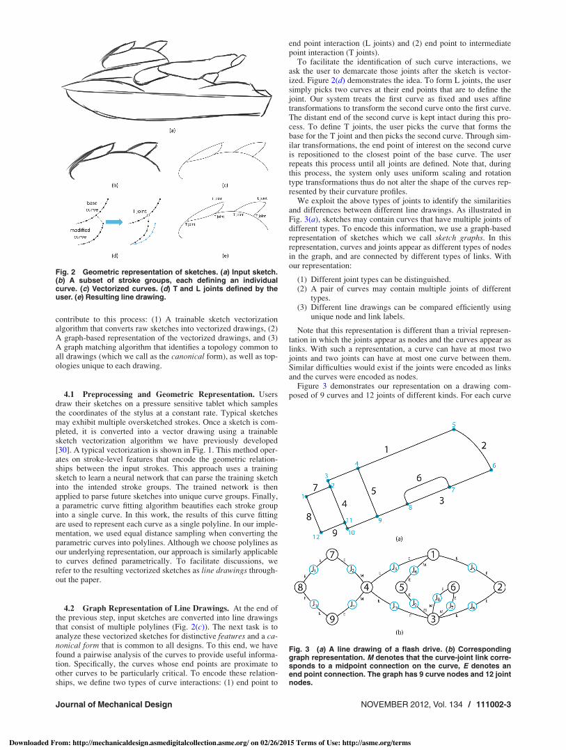
4.2 Graph Representation of Line Drawings. At the end ofthe previous step, input sketches are converted into line drawingsthat consist of multiple polylines (Fig. 2(c)). The next task is toanalyze these vectorized sketches for distinctive features and a ca-nonical form that is common to all designs. To this end, we havefound a pairwise analysis of the curves to provide useful informa-tion. Specifically, the curves whose end points are proximate toother curves to be particularly critical. To encode these relation-ships, we define two types of curve interactions: (1) end point to

end point interaction (L joints) and (2) end point to intermediatepoint interaction (T joints).

To facilitate the identification of such curve interactions, weask the user to demarcate those joints after the sketch is vector-ized. Figure 2(d) demonstrates the idea. To form L joints, the usersimply picks two curves at their end points that are to define thejoint. Our system treats the first curve as fixed and uses affinetransformations to transform the second curve onto the first curve.The distant end of the second curve is kept intact during this pro-cess. To define T joints, the user picks the curve that forms thebase for the T joint and then picks the second curve. Through sim-ilar transformations, the end point of interest on the second curveis repositioned to the closest point of the base curve. The userrepeats this process until all joints are defined. Note that, duringthis process, the system only uses uniform scaling and rotationtype transformations thus do not alter the shape of the curves rep-resented by their curvature profiles.

We exploit the above types of joints to identify the similaritiesand differences between different line drawings. As illustrated inFig. 3(a), sketches may contain curves that have multiple joints ofdifferent types. To encode this information, we use a graph-basedrepresentation of sketches which we call sketch graphs. In thisrepresentation, curves and joints appear as different types of nodesin the graph, and are connected by different types of links. Withour representation:

(1) Different joint types can be distinguished.(2) A pair of curves may contain multiple joints of different

types.(3) Different line drawings can be compared efficiently using

unique node and link labels.

Note that this representation is different than a trivial represen-tation in which the joints appear as nodes and the curves appear aslinks. With such a representation, a curve can have at most twojoints and two joints can have at most one curve between them.Similar difficulties would exist if the joints were encoded as linksand the curves were encoded as nodes.

Figure 3 demonstrates our representation on a drawing com-posed of 9 curves and 12 joints of different kinds. For each curve

Fig. 2 Geometric representation of sketches. (a) Input sketch.(b) A subset of stroke groups, each defining an individualcurve. (c) Vectorized curves. (d) T and L joints defined by theuser. (e) Resulting line drawing.

Fig. 3 (a) A line drawing of a flash drive. (b) Correspondinggraph representation. M denotes that the curve-joint link corre-sponds to a midpoint connection on the curve, E denotes anend point connection. The graph has 9 curve nodes and 12 jointnodes.

Journal of Mechanical Design NOVEMBER 2012, Vol. 134 / 111002-3


and joint, there is a unique node in the graph. For each jointbetween a pair of curves, the corresponding curve nodes are con-nected to the joint node. Multiple joint nodes may exist betweentwo curves nodes. The graph links connecting different types ofjoints (i.e., T or L joint) have different labels. If a joint is locatedalong the interior of a curve, the graph link between this joint andthe curve is labeled as M denoting a middle point. Similarly, if ajoint is located at an end point of a curve, the graph link is labeledas E denoting an end point. It should be noted that this choice of con-nections implies that curve nodes can only be connected to jointnodes, and vice versa. Thus, having a separate joint node in the graphallows a curve to be connected to multiple joints in the graph.

4.3 Topological Graph Matching. After vectorization andjoint formation, all sketches are converted into sketch graphs asdescribed above. In this phase, the aim is to find a canonical formcommon to all sketches, as well as design-specific features. Forthis purpose, we seek to partition each sketch graph into two sub-graphs, corresponding to a base graph representing the canonicalform, and a set of detail graphs unique to each sketch. Thesegraphs and their sizes are unknown a priori with only one con-strain that the base graphs of each sketch are topologically identi-cal. We use a graph-subgraph isomorphism algorithm todetermine the topologically identical (i.e., having exactly thesame node and link structure) subgraphs as candidates for the ca-nonical form. Among those, we choose the one which is also geo-metrically similar in all designs using a set of pairwise geometricsimilarity features.

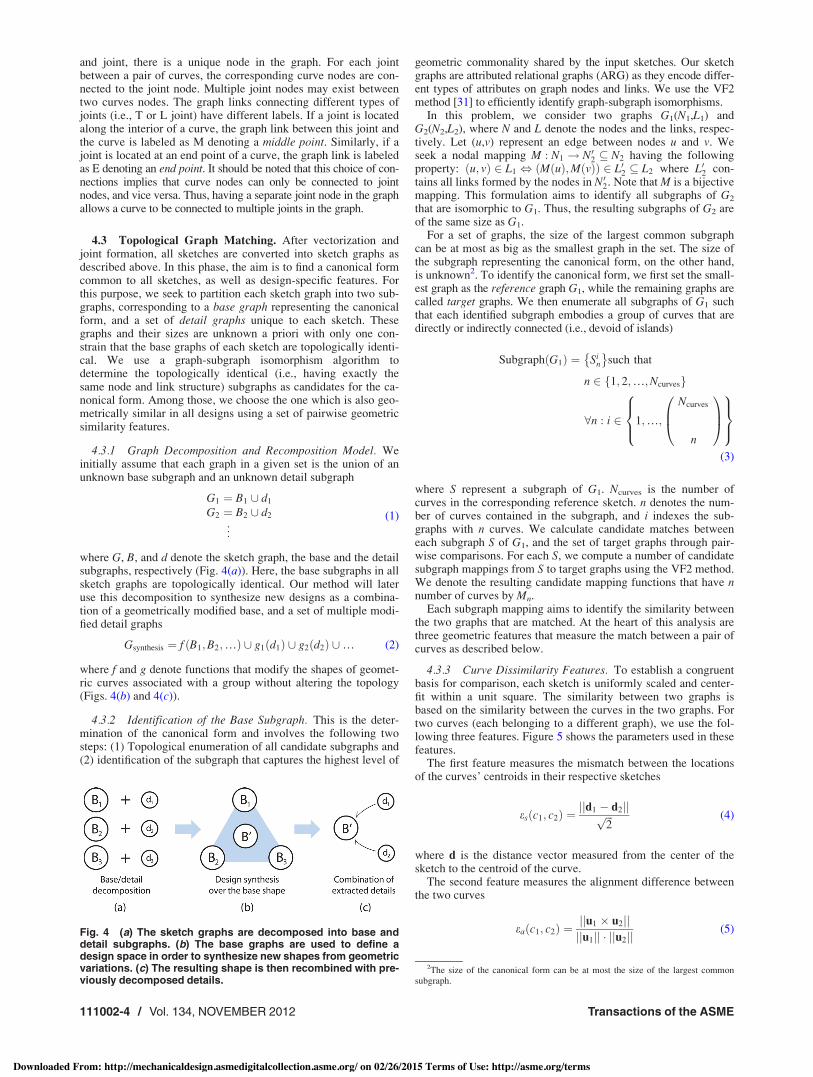
4.3.1 Graph Decomposition and Recomposition Model. Weinitially assume that each graph in a given set is the union of anunknown base subgraph and an unknown detail subgraph

G1 ! B1 [ d1

G2 ! B2 [ d2

..

.(1)

where G, B, and d denote the sketch graph, the base and the detailsubgraphs, respectively (Fig. 4(a)). Here, the base subgraphs in allsketch graphs are topologically identical. Our method will lateruse this decomposition to synthesize new designs as a combina-tion of a geometrically modified base, and a set of multiple modi-fied detail graphs

Gsynthesis ! f "B1;B2;…# [ g1"d1# [ g2"d2# [… (2)

where f and g denote functions that modify the shapes of geomet-ric curves associated with a group without altering the topology(Figs. 4(b) and 4(c)).

4.3.2 Identification of the Base Subgraph. This is the deter-mination of the canonical form and involves the following twosteps: (1) Topological enumeration of all candidate subgraphs and(2) identification of the subgraph that captures the highest level of

geometric commonality shared by the input sketches. Our sketchgraphs are attributed relational graphs (ARG) as they encode differ-ent types of attributes on graph nodes and links. We use the VF2method [31] to efficiently identify graph-subgraph isomorphisms.

In this problem, we consider two graphs G1(N1,L1) andG2(N2,L2), where N and L denote the nodes and the links, respec-tively. Let (u,v) represent an edge between nodes u and v. Weseek a nodal mapping M : N1 ! N02 $ N2 having the followingproperty: u; v" # 2 L1 , M u" #;M v" #" # 2 L02 $ L2 where L02 con-tains all links formed by the nodes in N02. Note that M is a bijectivemapping. This formulation aims to identify all subgraphs of G2

that are isomorphic to G1. Thus, the resulting subgraphs of G2 areof the same size as G1.

For a set of graphs, the size of the largest common subgraphcan be at most as big as the smallest graph in the set. The size ofthe subgraph representing the canonical form, on the other hand,is unknown2. To identify the canonical form, we first set the small-est graph as the reference graph G1, while the remaining graphs arecalled target graphs. We then enumerate all subgraphs of G1 suchthat each identified subgraph embodies a group of curves that aredirectly or indirectly connected (i.e., devoid of islands)

Subgraph"G1# ! Sin

! "such that

n 2 f1; 2;…;Ncurvesg

8n : i 2 1;…;

Ncurves

n

0

B@

1

CA

8><

>:

9>=

>;

(3)

where S represent a subgraph of G1. Ncurves is the number ofcurves in the corresponding reference sketch. n denotes the num-ber of curves contained in the subgraph, and i indexes the sub-graphs with n curves. We calculate candidate matches betweeneach subgraph S of G1, and the set of target graphs through pair-wise comparisons. For each S, we compute a number of candidatesubgraph mappings from S to target graphs using the VF2 method.We denote the resulting candidate mapping functions that have nnumber of curves by Mn.

Each subgraph mapping aims to identify the similarity betweenthe two graphs that are matched. At the heart of this analysis arethree geometric features that measure the match between a pair ofcurves as described below.

4.3.3 Curve Dissimilarity Features. To establish a congruentbasis for comparison, each sketch is uniformly scaled and center-fit within a unit square. The similarity between two graphs isbased on the similarity between the curves in the two graphs. Fortwo curves (each belonging to a different graph), we use the fol-lowing three features. Figure 5 shows the parameters used in thesefeatures.

The first feature measures the mismatch between the locationsof the curves’ centroids in their respective sketches

es"c1; c2# !jjd1 % d2jj###

2p (4)

where d is the distance vector measured from the center of thesketch to the centroid of the curve.

The second feature measures the alignment difference betweenthe two curves

ea"c1; c2# !jju1 & u2jjjju1jj ' jju2jj

(5)Fig. 4 (a) The sketch graphs are decomposed into base anddetail subgraphs. (b) The base graphs are used to define adesign space in order to synthesize new shapes from geometricvariations. (c) The resulting shape is then recombined with pre-viously decomposed details.

2The size of the canonical form can be at most the size of the largest commonsubgraph.



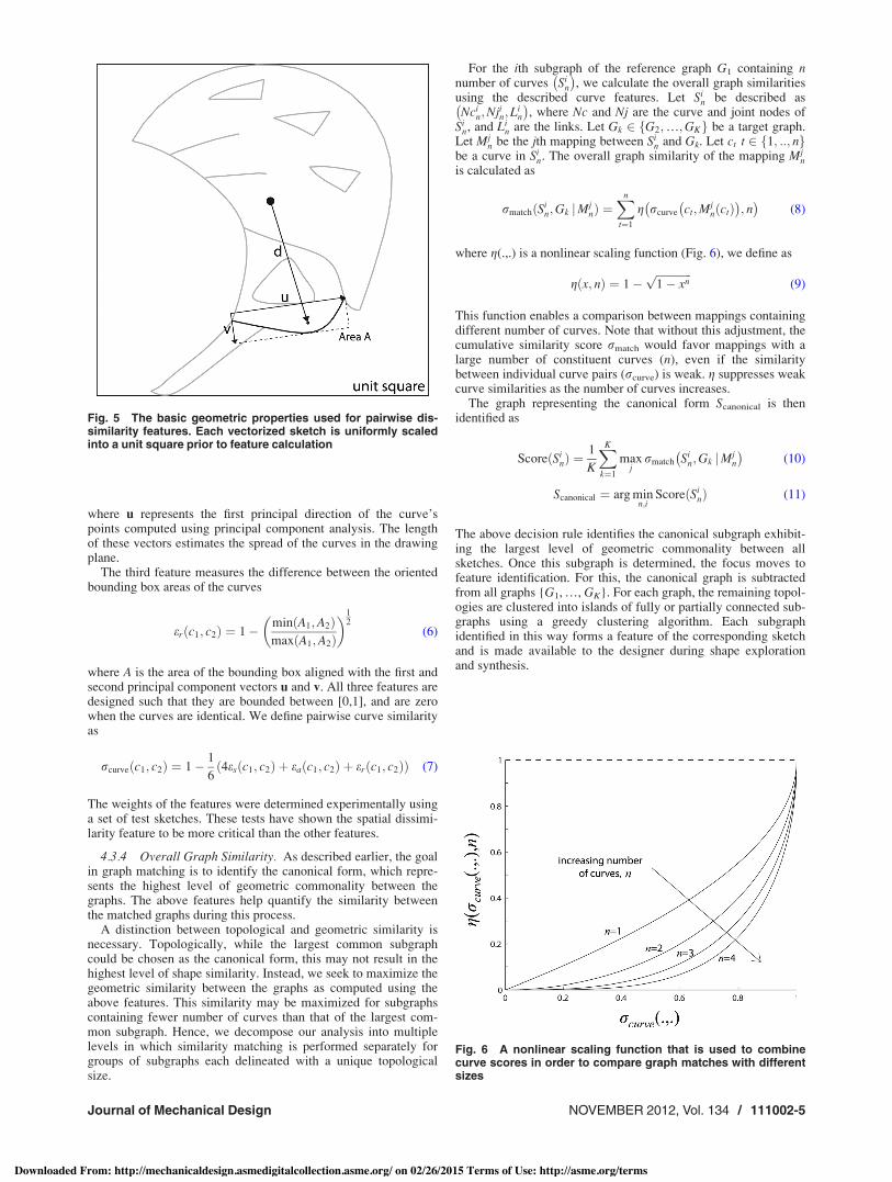
where u represents the first principal direction of the curve’spoints computed using principal component analysis. The lengthof these vectors estimates the spread of the curves in the drawingplane.

The third feature measures the difference between the orientedbounding box areas of the curves

er"c1; c2# ! 1% min"A1;A2#max"A1;A2#

$ %12

(6)

where A is the area of the bounding box aligned with the first andsecond principal component vectors u and v. All three features aredesigned such that they are bounded between [0,1], and are zerowhen the curves are identical. We define pairwise curve similarityas

rcurve"c1; c2# ! 1% 1

64es"c1; c2# ( ea"c1; c2# ( er"c1; c2#" # (7)

The weights of the features were determined experimentally usinga set of test sketches. These tests have shown the spatial dissimi-larity feature to be more critical than the other features.

4.3.4 Overall Graph Similarity. As described earlier, the goalin graph matching is to identify the canonical form, which repre-sents the highest level of geometric commonality between thegraphs. The above features help quantify the similarity betweenthe matched graphs during this process.

A distinction between topological and geometric similarity isnecessary. Topologically, while the largest common subgraphcould be chosen as the canonical form, this may not result in thehighest level of shape similarity. Instead, we seek to maximize thegeometric similarity between the graphs as computed using theabove features. This similarity may be maximized for subgraphscontaining fewer number of curves than that of the largest com-mon subgraph. Hence, we decompose our analysis into multiplelevels in which similarity matching is performed separately forgroups of subgraphs each delineated with a unique topologicalsize.

For the ith subgraph of the reference graph G1 containing nnumber of curves Si

n

& ', we calculate the overall graph similarities

using the described curve features. Let Sin be described as

Ncin;Njin;L

in

& ', where Nc and Nj are the curve and joint nodes of

Sin, and Li

n are the links. Let Gk 2 fG2;…;GKg be a target graph.Let Mj

n be the jth mapping between Sin and Gk. Let ct t 2 f1; ::; ng

be a curve in Sin. The overall graph similarity of the mapping Mj

nis calculated as

rmatch"Sin;Gk jMj

n# !Xn

t!1

g rcurve ct;Mjn"ct#

& '; n

& '(8)

where g(.,.) is a nonlinear scaling function (Fig. 6), we define as

g"x; n# ! 1%#############1% xnp

(9)

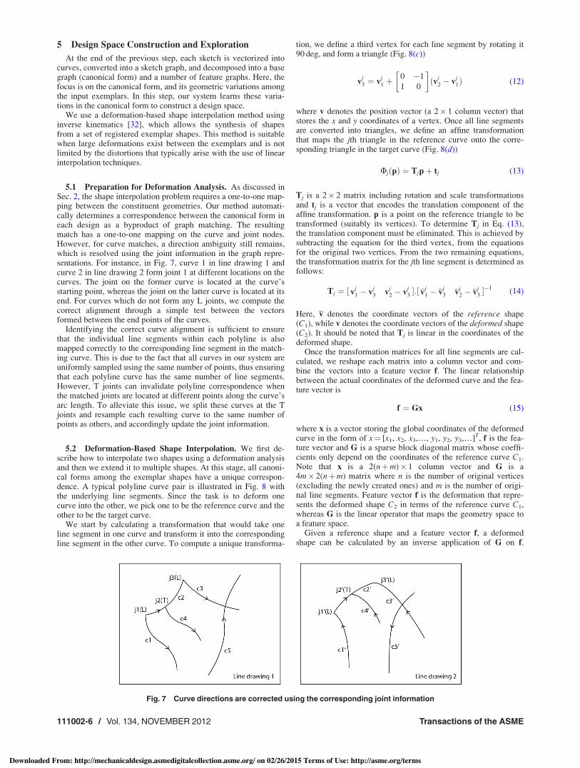
This function enables a comparison between mappings containingdifferent number of curves. Note that without this adjustment, thecumulative similarity score rmatch would favor mappings with alarge number of constituent curves (n), even if the similaritybetween individual curve pairs (rcurve) is weak. g suppresses weakcurve similarities as the number of curves increases.

The graph representing the canonical form Scanonical is thenidentified as

Score"Sin# !

1

K

XK

k!1

maxj

rmatch Sin;Gk jMj

n

& '(10)

Scanonical ! arg minn;i

Score"Sin# (11)

The above decision rule identifies the canonical subgraph exhibit-ing the largest level of geometric commonality between allsketches. Once this subgraph is determined, the focus moves tofeature identification. For this, the canonical graph is subtractedfrom all graphs {G1, …, GK}. For each graph, the remaining topol-ogies are clustered into islands of fully or partially connected sub-graphs using a greedy clustering algorithm. Each subgraphidentified in this way forms a feature of the corresponding sketchand is made available to the designer during shape explorationand synthesis.

Fig. 5 The basic geometric properties used for pairwise dis-similarity features. Each vectorized sketch is uniformly scaledinto a unit square prior to feature calculation

Fig. 6 A nonlinear scaling function that is used to combinecurve scores in order to compare graph matches with differentsizes



5 Design Space Construction and Exploration

At the end of the previous step, each sketch is vectorized intocurves, converted into a sketch graph, and decomposed into a basegraph (canonical form) and a number of feature graphs. Here, thefocus is on the canonical form, and its geometric variations amongthe input exemplars. In this step, our system learns these varia-tions in the canonical form to construct a design space.

We use a deformation-based shape interpolation method usinginverse kinematics [32], which allows the synthesis of shapesfrom a set of registered exemplar shapes. This method is suitablewhen large deformations exist between the exemplars and is notlimited by the distortions that typically arise with the use of linearinterpolation techniques.

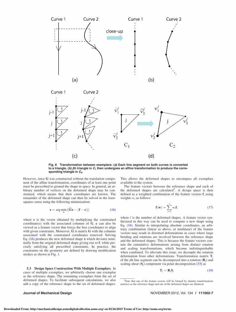
5.1 Preparation for Deformation Analysis. As discussed inSec. 2, the shape interpolation problem requires a one-to-one map-ping between the constituent geometries. Our method automati-cally determines a correspondence between the canonical form ineach design as a byproduct of graph matching. The resultingmatch has a one-to-one mapping on the curve and joint nodes.However, for curve matches, a direction ambiguity still remains,which is resolved using the joint information in the graph repre-sentations. For instance, in Fig. 7, curve 1 in line drawing 1 andcurve 2 in line drawing 2 form joint 1 at different locations on thecurves. The joint on the former curve is located at the curve’sstarting point, whereas the joint on the latter curve is located at itsend. For curves which do not form any L joints, we compute thecorrect alignment through a simple test between the vectorsformed between the end points of the curves.

Identifying the correct curve alignment is sufficient to ensurethat the individual line segments within each polyline is alsomapped correctly to the corresponding line segment in the match-ing curve. This is due to the fact that all curves in our system areuniformly sampled using the same number of points, thus ensuringthat each polyline curve has the same number of line segments.However, T joints can invalidate polyline correspondence whenthe matched joints are located at different points along the curve’sarc length. To alleviate this issue, we split these curves at the Tjoints and resample each resulting curve to the same number ofpoints as others, and accordingly update the joint information.

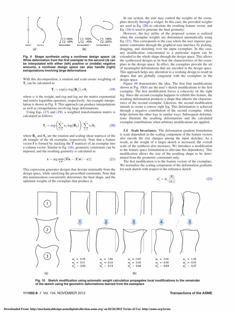
5.2 Deformation-Based Shape Interpolation. We first de-scribe how to interpolate two shapes using a deformation analysisand then we extend it to multiple shapes. At this stage, all canoni-cal forms among the exemplar shapes have a unique correspon-dence. A typical polyline curve pair is illustrated in Fig. 8 withthe underlying line segments. Since the task is to deform onecurve into the other, we pick one to be the reference curve and theother to be the target curve.

We start by calculating a transformation that would take oneline segment in one curve and transform it into the correspondingline segment in the other curve. To compute a unique transforma-

tion, we define a third vertex for each line segment by rotating it90 deg, and form a triangle (Fig. 8(c))

vj3 ! vj

1 (0 %11 0

( )"vj

2 % vj1# (12)

where v denotes the position vector (a 2& 1 column vector) thatstores the x and y coordinates of a vertex. Once all line segmentsare converted into triangles, we define an affine transformationthat maps the jth triangle in the reference curve onto the corre-sponding triangle in the target curve (Fig. 8(d))

Uj"p# ! Tjp( tj (13)

Tj is a 2& 2 matrix including rotation and scale transformationsand tj is a vector that encodes the translation component of theaffine transformation. p is a point on the reference triangle to betransformed (suitably its vertices). To determine Tj in Eq. (13),the translation component must be eliminated. This is achieved bysubtracting the equation for the third vertex, from the equationsfor the original two vertices. From the two remaining equations,the transformation matrix for the jth line segment is determined asfollows:

Tj ! ) vj1 % vj

3 vj2 % vj

3*:) vj

1 % vj3 vj

2 % vj3*%1 (14)

Here, v denotes the coordinate vectors of the reference shape(C1), while v denotes the coordinate vectors of the deformed shape(C2). It should be noted that Tj is linear in the coordinates of thedeformed shape.

Once the transformation matrices for all line segments are cal-culated, we reshape each matrix into a column vector and com-bine the vectors into a feature vector f. The linear relationshipbetween the actual coordinates of the deformed curve and the fea-ture vector is

f ! Gx (15)

where x is a vector storing the global coordinates of the deformedcurve in the form of x! [x1, x2, x3,…, y1, y2, y3,…]T, f is the fea-ture vector and G is a sparse block diagonal matrix whose coeffi-cients only depend on the coordinates of the reference curve C1.Note that x is a 2(n(m)& 1 column vector and G is a4m& 2(n(m) matrix where n is the number of original vertices(excluding the newly created ones) and m is the number of origi-nal line segments. Feature vector f is the deformation that repre-sents the deformed shape C2 in terms of the reference curve C1,whereas G is the linear operator that maps the geometry space toa feature space.

Given a reference shape and a feature vector f, a deformedshape can be calculated by an inverse application of G on f.

Fig. 7 Curve directions are corrected using the corresponding joint information



However, since G was constructed without the translation compo-nent of the affine transformation, coordinates of at least one pointmust be prescribed to ground the shape in space. In general, an ar-bitrary number of vertices on the deformed shape may be con-strained, which means that their coordinates are known. Theremainder of the deformed shape can then be solved in the least-squares sense using the following minimization:

x ! arg minxjjGx% f % c" #jj (16)

where c is the vector obtained by multiplying the constrainedcoordinate(s) with the associated columns of G. c can also beviewed as a feature vector that forces the free coordinates to alignwith given constraints. Moreover, G is matrix G with the columnsassociated with the constrained coordinates removed. SolvingEq. (16) produces the new deformed shape x which deviates mini-mally from the original deformed shape giving rise to f, while pre-cisely satisfying all prescribed constraints. In practice, theconstraints on the geometry are defined by drawing modificationstrokes as shown in Fig. 1.

5.3 Design Space Construction With Multiple Exemplars. Incases of multiple exemplars, we arbitrarily choose one exemplaras the reference shape. The remaining exemplars form the set ofdeformed shapes. To facilitate subsequent calculations, we alsoadd a copy of the reference shape to the set of deformed shapes.

This allows the deformed shapes to encompass all exemplarsavailable to the system.

The feature vectors between the reference shape and each ofthe deformed shapes are calculated3. A design space is thendefined as a weighted combination of the feature vectors fi usingweights wi as follows:

f"w# !Xl

i!1

wif i (17)

where l is the number of deformed shapes. A feature vector syn-thesized in this way can be used to compute a new shape usingEq. (16). Similar to interpolating absolute coordinates, an arbi-trary combination (linear as above, or nonlinear) of the featurevectors may result in distorted deformations in cases where largebending and rotations are involved between the reference shapeand the deformed shapes. This is because the feature vectors con-tain the cumulative deformations arising from distinct rotationand scaling transformations, which become indistinguishablewhen combined. To alleviate this issue, we decouple the rotationdeformation from other deformations. Transformation matrix Tj

of the jth line segment can be decomposed into a rotation (Rj) andscaling-shear (Sj) component via polar decomposition [33] as

Tj ! RjSj (18)

Fig. 8 Transformation between exemplars: (a) Each line segment on both curves is convertedto a triangle. (b) jth triangle in C1 then undergoes an affine transformation to produce the corre-sponding triangle in C2.

3Note that one of the feature vectors will be formed by identity transformationmatrices as the reference shape and one of the deformed shapes are identical.



With this decomposition, a rotation and scale-aware weighting ofTj can be calculated as

Tj ! exp w log Rj

& '& ':wSj (19)

where w is the weight, and exp and log are the matrix exponentialand matrix logarithm operators, respectively. An example interpo-lation is shown in Fig. 9. This approach can produce interpolationsas well as extrapolations involving large deformations.

Using Eqs. (17) and (19), a weighted transformation matrix iscalculated as follows:

Tj ! expXl

i!1

wi log Rij

& ' !

:Xl

i!1

wiSij (20)

where Rij and Sij are the rotation and scaling-shear matrices of thejth triangle of the ith exemplar, respectively. Note that a featurevector f is formed by stacking the T matrices of an exemplar intoa column vector. Similar to Eq. (16), geometric constraints can beimposed, and the resulting geometry is calculated as

x ! arg minx;wjjGx% f"w# % c" #jj (21)

This expression generates designs that deviate minimally from thedesign space, while satisfying the prescribed constraints. Note thatthis minimization concurrently determines the final shape, and theoptimum weights of the exemplars that produce it.

In our system, the user may control the weights of the exem-plars directly through a widget. In this case, the provided weightsare used in Eq. (20) to calculate the resulting feature vector, andEq. (16) is used to generate the final geometry.

However, the key utility of the proposed system is realizedwhen the exemplar weights are determined automatically usingEq. (21). This corresponds to the case where the user imposes geo-metric constraints through the graphical user interface by picking,dragging, and sketching over the input exemplars. In this case,any modification concentrated to a particular region can beextended to the whole shape through the design space. This allowsthe synthesized designs to be bear the characteristics of the exem-plars in the design space. In effect, the exemplars provide the setof meaningful deformations that are encoded in the design space.This approach helps any alteration to a working design to result inshapes that are globally congruent with the exemplars in thedesign space.

Figure 10 demonstrates the idea. The first four modificationsshown in Fig. 10(b) are the user’s sketch modifications to the firstexemplar. The first modification forces a concavity on the rightleg. Since the second exemplar happens to exhibit this feature, theresulting deformation produces a shape that inherits the character-istics of the second exemplar. Likewise, the second modificationintends to create a convex right leg. This deformation is achievedthrough a negative contribution of the second exemplar, whichhelps deform the other legs in similar ways. Subsequent deforma-tions illustrate the resulting deformations and the calculatedexemplar contributions when arbitrary modifications are applied.

5.4 Scale Invariance. The deformation gradient formulationis scale dependent as the scaling component of the feature vectorsalso encode the size changes among the input sketches. As aresult, as the weight of a larger sketch is increased, the overallscale of the synthesis also increases. We introduce a modificationto the feature space formulation to alleviate this dependency. Thismodification allows the size of the resulting shape to be deter-mined from the geometric constraints only.

The first modification is to the feature vectors of the exemplars.We normalize the scaling component of the deformation gradientsfor each sketch with respect to the reference sketch

w0i ! wijjIjjjjwijj

(22)

Fig. 9 Shape synthesis using a nonlinear design space: (a)While deformation from the first exemplar to the second (b) canbe interpolated with either (left) positive or (middle) negativeamounts, a nonlinear design space can also handle (right)extrapolations involving large deformations

Fig. 10 Sketch modification using automatic weight calculation propagates local modifications to the remainderof the sketch using the geometric deformations learned from the exemplars



where w0i and wi are the normalized and original scaling featurevectors, which are constructed the same way as the features vec-tors. I is the scaling feature vector which is constructed from iden-tity transformation matrices, and k.k is the matrix norm operator.This normalization scales the exemplars to the scale of the refer-ence sketch such that the scale transformation between eachexemplar to the reference shape is an identity matrix. This nor-malization also helps preserve the overall size of the referenceshape when only one point is constrained. Note that at least twopoints are required to uniquely define the size. In these cases, weuse Eq. (16) with the normalized feature vectors.

For cases in which the user constrains more than one point andassigns the exemplar weights manually (i.e., f(w) is known), weintroduce a free scaling parameter to Eq. (16) as

x ! arg minx;ajjGx% af"w# % c" #jj (23)

where a is the unknown scaling parameter. This scaling parameterintroduces an additional degree of freedom that allows a uniformscaling of the final shape in cases where the exemplar weights areexternally prescribed.

In cases where the user constrains more than one point and letsthe system calculate the set of weights, the introduction of a is nolonger necessary. This is because the presence of the referenceshape in the set of deformed shapes allows the associated weightcomputed by Eq. (21) to serve as the free scaling parameter.

5.5 Design Space Exploration and Shape Optimization. Oursystem presents the canonical form of the reference design asthe initial shape (i.e., a working design). For design exploration,the user may impose geometric constraints and attach one ormore of the identified features to the working design. The geomet-ric constraints can be added and modified by picking/movinggestures of the stylus, or by directly sketching over the workingdesign. In case of sketch modifications, our system automaticallydetermines the portions of the shape to be modified using a prox-imity check. It then moves the points selected for modificationonto the modification strokes. These points are subsequentlytreated as constrained points. The user may also pick one ormore design-specific features and attach them to the workingmodel. For each added feature, the user first picks a point onthe feature and then picks an attachment point on the workingdesign. The user may also define further constraints on thefeatures.

Shape variations can be achieved through a manual or auto-matic control of the exemplar weights. In the first case, the useradjusts the weights of each exemplar through a widget, whichinteractively changes the shape. In the second case, the user speci-fies the geometric constraints. The resulting shape is then deter-mined according to Eq. (21).

Our approach is also conducive to constrained shape optimiza-tion when geometric objective functions are specified. Currentshape optimization techniques typically require parameterizedgeometries. Often times, this parameterization is not trivial andhas to be established by the designers. In our approach, the graph-based sketch analysis and the subsequent design space construc-tion alleviates this need. During optimization, the exemplarweights serve as the optimization parameters, whose combinationleads to an optimum design. Section 7 demonstrates this capabilityon different examples.

6 Computational Complexity Analysis

The computational complexity of our system is dictated primar-ily by the canonical form identification and detail extraction step,as graph matching is an nondeterministic polynomial-time (NP)-complete problem.

Let ne! total number of exemplars, nc!maximum number ofcurves in an exemplar, and nj!maximum number of joints in an

exemplar. As described earlier, we calculate and evaluate allpossible graph matches between a reference sketch and all othersketches. In the graph representation, the number of nodes, N, isthe summation of number of curves and joints (i.e., nc( nj). Weassume the worst case scenario of all nodes connecting to oneanother. Thus, the number of connected subgraphs of the refer-ence graph to be matched with other graphs is 2N% 1. For eachsubgraph, the VF2 algorithm determines graph matches at a costof O(N!N) [31]. Combined, the worst case complexity of this stepis O(N!N2N).

The design space exploration step is far less demanding. Equa-tions (16) and (21) both require the solution of a linear systemwhich can be efficiently done using QR, Cholesky matrix decom-positions or similar methods. Our implementation works at inter-active speeds that allow users to work fluently. Detaileddiscussion of the computational complexity of this step can befound in Ref. [32].

7 Example Design Cases

Secs. 7.1 and 7.2, we demonstrate (1) canonical form identifica-tion, detail extraction, shape exploration, and synthesis and (2)constrained shape optimization under engineering objectives.

7.1 Canonical Form Identification, Detail Extraction,Shape Exploration, and Synthesis. We demonstrate our methodwith four design cases. The first three examples are user-drawnand are simplified with the stroke clustering and vectorizationmethod described earlier. The last example is created with asketch-based 3D modeling interface, thus did not require curvevectorization.

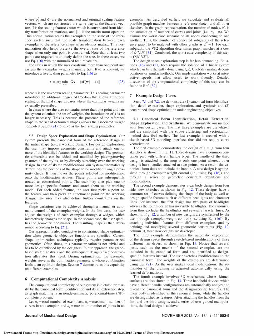
The first example demonstrates the design of a mug from foursketches as shown in Fig. 11. These designs have a common con-tainer part with different handle types. The handle of the thirddesign is attached to the mug at only one point whereas otherdesigns have handles attached at two points. As a result, the ca-nonical form does not include the handle. A new design is synthe-sized through exemplar weight control (i.e., using Eq. (16)), andthrough a series of geometric constraint definitions andmodifications.

The second example demonstrates a car body design from fourside view sketches as shown in Fig. 12. These designs have acommon set of curves defining the shape of the body as well asdesign-specific features such as different headlights and characterlines. For instance, the first design has two pairs of headlightswhereas the fourth design has no visible headlights. The canonicalform thus excludes the headlights and several character lines. Asshown in Fig. 12, a number of new designs are synthesized by theuser through exemplar weight control (i.e., using Eq. (16)). Byattaching individual features from different exemplars, and bydefining and modifying several geometric constraints (Fig. 12,column 3), three new designs are developed.

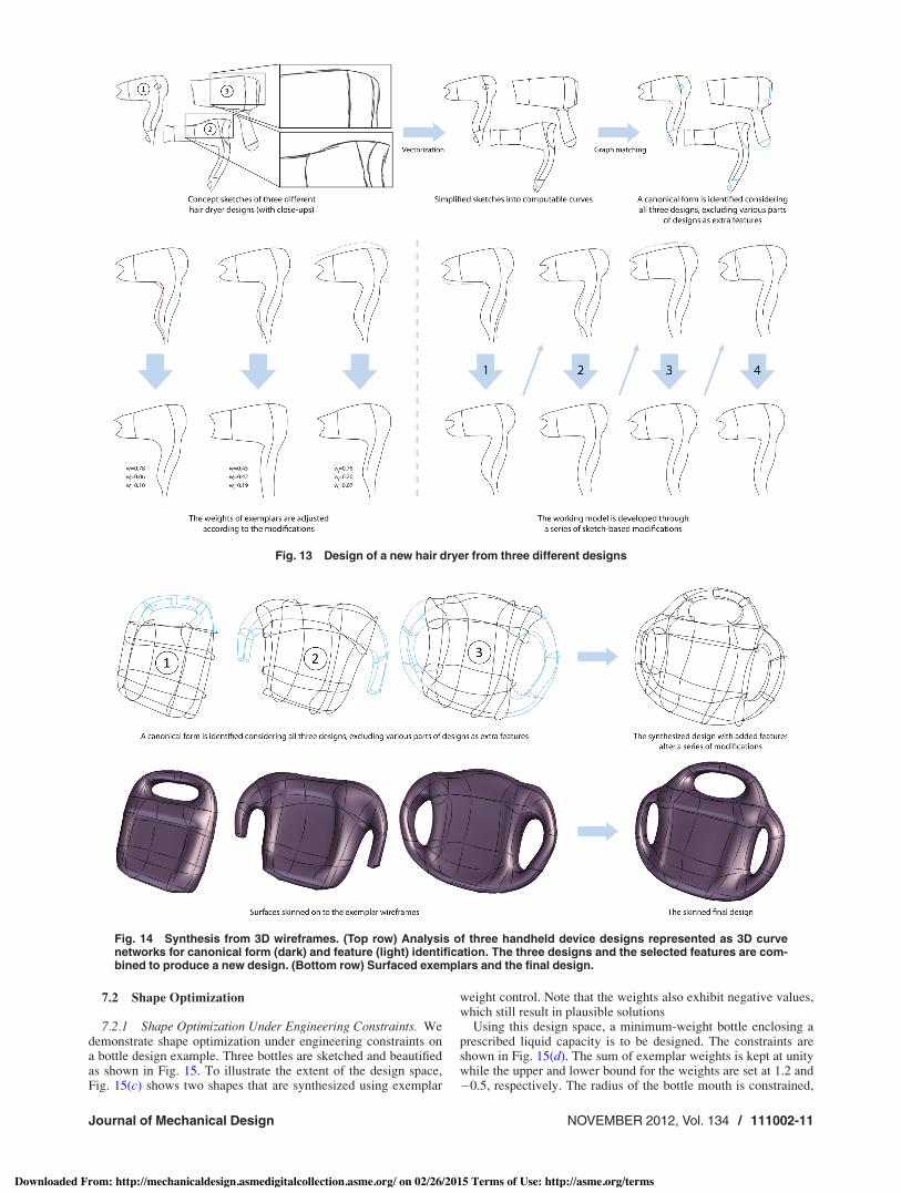
The third example demonstrates the automatic explorationof the design space through sketch-based modifications of threedifferent hair dryers as shown in Fig. 13. Notice that severalparts, such as the nozzle of the second exemplar, are notincluded in the canonical form and are identified as design-specific features instead. The user sketches modifications to thecanonical form. The weights of the exemplars are determinedusing Eq. (21). As the user makes local modifications, the re-mainder of the drawing is adjusted automatically using thelearned deformations.

The fourth example involves 3D wireframes, whose skinnedsurfaces are also shown in Fig. 14. Three handheld devices whichhave different handle configurations are automatically analyzed toreveal the canonical form and the design-specific features. Themain body is identified as the canonical form, while the handlesare distinguished as features. After attaching the handles from thefirst and the third designs, and a series of user-guided manipula-tions, the final design is achieved.



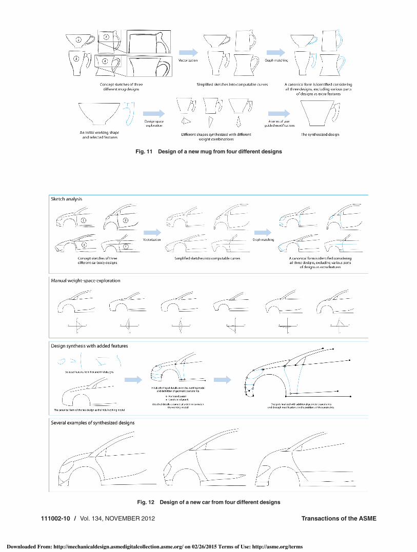
Fig. 12 Design of a new car from four different designs

Fig. 11 Design of a new mug from four different designs



7.2 Shape Optimization

7.2.1 Shape Optimization Under Engineering Constraints. Wedemonstrate shape optimization under engineering constraints ona bottle design example. Three bottles are sketched and beautifiedas shown in Fig. 15. To illustrate the extent of the design space,Fig. 15(c) shows two shapes that are synthesized using exemplar

weight control. Note that the weights also exhibit negative values,which still result in plausible solutions

Using this design space, a minimum-weight bottle enclosing aprescribed liquid capacity is to be designed. The constraints areshown in Fig. 15(d). The sum of exemplar weights is kept at unitywhile the upper and lower bound for the weights are set at 1.2 and%0.5, respectively. The radius of the bottle mouth is constrained,

Fig. 13 Design of a new hair dryer from three different designs

Fig. 14 Synthesis from 3D wireframes. (Top row) Analysis of three handheld device designs represented as 3D curvenetworks for canonical form (dark) and feature (light) identification. The three designs and the selected features are com-bined to produce a new design. (Bottom row) Surfaced exemplars and the final design.



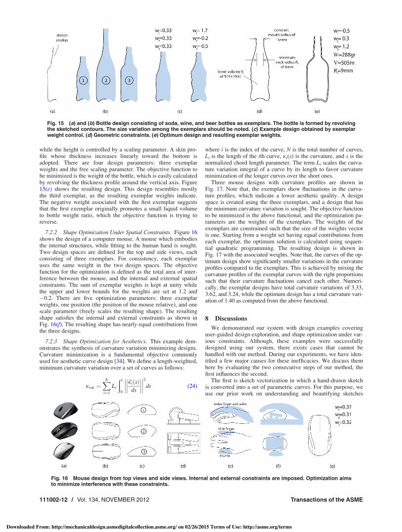
while the height is controlled by a scaling parameter. A skin pro-file whose thickness increases linearly toward the bottom isadopted. There are four design parameters: three exemplarweights and the free scaling parameter. The objective function tobe minimized is the weight of the bottle, which is easily calculatedby revolving the thickness profile around the vertical axis. Figure15(e) shows the resulting design. This design resembles mostlythe third exemplar, as the resulting exemplar weights indicate.The negative weight associated with the first exemplar suggeststhat the first exemplar originally promotes a small liquid volumeto bottle weight ratio, which the objective function is trying toreverse.

7.2.2 Shape Optimization Under Spatial Constraints. Figure 16shows the design of a computer mouse. A mouse which embodiesthe internal structures, while fitting to the human hand is sought.Two design spaces are defined for the top and side views, eachconsisting of three exemplars. For consistency, each exemplaruses the same weight in the two design spaces. The objectivefunction for the optimization is defined as the total area of inter-ference between the mouse, and the internal and external spatialconstraints. The sum of exemplar weights is kept at unity whilethe upper and lower bounds for the weights are set at 1.2 and%0.2. There are five optimization parameters: three exemplarweights, one position (the position of the mouse relative), and onescale parameter (freely scales the resulting shape). The resultingshape satisfies the internal and external constraints as shown inFig. 16(f). The resulting shape has nearly equal contributions fromthe three designs.

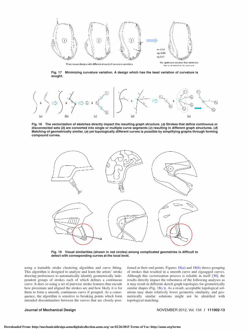
7.2.3 Shape Optimization for Aesthetics. This example dem-onstrates the synthesis of curvature variation minimizing designs.Curvature minimization is a fundamental objective commonlyused for aesthetic curve design [34]. We define a length-weighted,minimum curvature variation over a set of curves as follows:

jvar !XN

i!1

Li

*1

0

~ji"s#ds

++++

++++

++++

++++2

ds (24)

where i is the index of the curve, N is the total number of curves,Li is the length of the ith curve, ji(s) is the curvature, and s is thenormalized chord length parameter. The term Li scales the curva-ture variation integral of a curve by its length to favor curvatureminimization of the longer curves over the short ones.

Three mouse designs with curvature profiles are shown inFig. 17. Note that, the exemplars show fluctuations in the curva-ture profiles, which indicate a lower aesthetic quality. A designspace is created using the three exemplars, and a design that hasthe minimum curvature variation is sought. The objective functionto be minimized is the above functional, and the optimization pa-rameters are the weights of the exemplars. The weights of theexemplars are constrained such that the size of the weights vectoris one. Starting from a weight set having equal contributions fromeach exemplar, the optimum solution is calculated using sequen-tial quadratic programming. The resulting design is shown inFig. 17 with the associated weights. Note that, the curves of the op-timum design show significantly smaller variations in the curvatureprofiles compared to the exemplars. This is achieved by mixing thecurvature profiles of the exemplar curves with the right proportionssuch that their curvature fluctuations cancel each other. Numeri-cally, the exemplar designs have total curvature variations of 3.33,3.62, and 3.24, while the optimum design has a total curvature vari-ation of 1.40 as computed from the above functional.

8 Discussions

We demonstrated our system with design examples coveringuser-guided design exploration, and shape optimization under var-ious constraints. Although, these examples were successfullydesigned using our system, there exists cases that cannot behandled with our method. During our experiments, we have iden-tified a few major causes for these inefficacies. We discuss themhere by evaluating the two consecutive steps of our method, thefirst influences the second.

The first is sketch vectorization in which a hand-drawn sketchis converted into a set of parametric curves. For this purpose, weuse our prior work on understanding and beautifying sketches

Fig. 15 (a) and (b) Bottle design consisting of soda, wine, and beer bottles as exemplars. The bottle is formed by revolvingthe sketched contours. The size variation among the exemplars should be noted. (c) Example design obtained by exemplarweight control. (d) Geometric constraints. (e) Optimum design and resulting exemplar weights.

Fig. 16 Mouse design from top views and side views. Internal and external constraints are imposed. Optimization aimsto minimize interference with these constraints.



using a trainable stroke clustering algorithm and curve fitting.This algorithm is designed to analyze and learn the artists’ strokedrawing preferences to automatically identify geometrically inde-pendent groups of strokes each of which defines a continuouscurve. It does so using a set of pairwise stroke features that encodehow proximate and aligned the strokes are and how likely it is forthem to form a smooth, continuous curve if grouped. As a conse-quence, the algorithm is sensitive to breaking points which formintended discontinuities between the curves that are closely posi-

tioned at their end points. Figures 18(a) and 18(b) shows groupingof strokes that resulted in a smooth curve and zigzagged curves.Although this vectorization process is reliable in itself [30], theresults directly impact the robustness of the following analyses asit may result in different sketch graph topologies for geometricallysimilar shapes (Fig. 18(c)). As a result, acceptable topological sol-utions may share relatively lower geometric similarity, and geo-metrically similar solutions might not be identified withtopological matching.

Fig. 17 Minimizing curvature variation. A design which has the least variation of curvature issought.

Fig. 18 The vectorization of sketches directly impact the resulting graph structure. (a) Strokes that define continuous ordisconnected sets (b) are converted into single or multiple curve segments (c) resulting in different graph structures. (d)Matching of geometrically similar, (e) yet topologically different curves is possible by simplifying graphs through formingcompound curves.

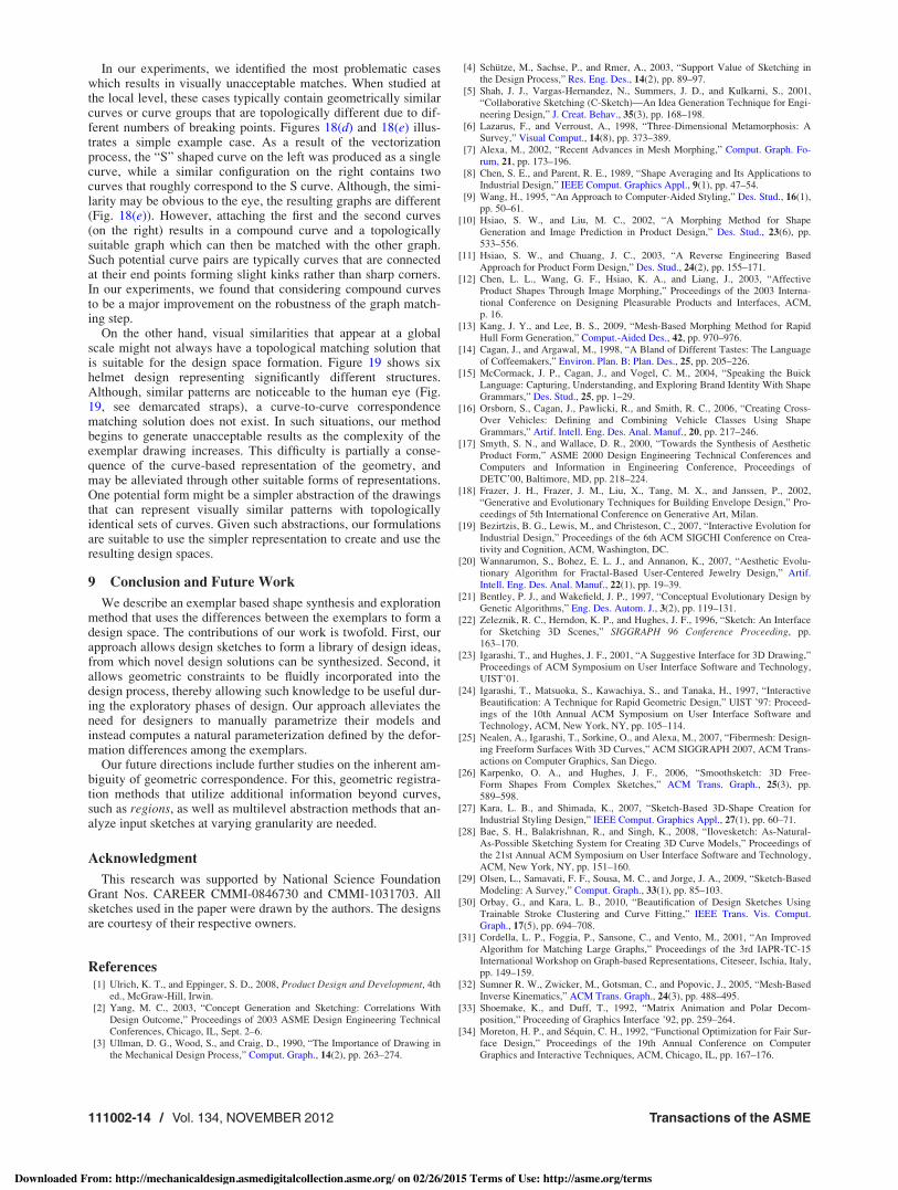
Fig. 19 Visual similarities (shown in red circles) among complicated geometries is difficult todetect with corresponding curves at the local level.



In our experiments, we identified the most problematic caseswhich results in visually unacceptable matches. When studied atthe local level, these cases typically contain geometrically similarcurves or curve groups that are topologically different due to dif-ferent numbers of breaking points. Figures 18(d) and 18(e) illus-trates a simple example case. As a result of the vectorizationprocess, the “S” shaped curve on the left was produced as a singlecurve, while a similar configuration on the right contains twocurves that roughly correspond to the S curve. Although, the simi-larity may be obvious to the eye, the resulting graphs are different(Fig. 18(e)). However, attaching the first and the second curves(on the right) results in a compound curve and a topologicallysuitable graph which can then be matched with the other graph.Such potential curve pairs are typically curves that are connectedat their end points forming slight kinks rather than sharp corners.In our experiments, we found that considering compound curvesto be a major improvement on the robustness of the graph match-ing step.

On the other hand, visual similarities that appear at a globalscale might not always have a topological matching solution thatis suitable for the design space formation. Figure 19 shows sixhelmet design representing significantly different structures.Although, similar patterns are noticeable to the human eye (Fig.19, see demarcated straps), a curve-to-curve correspondencematching solution does not exist. In such situations, our methodbegins to generate unacceptable results as the complexity of theexemplar drawing increases. This difficulty is partially a conse-quence of the curve-based representation of the geometry, andmay be alleviated through other suitable forms of representations.One potential form might be a simpler abstraction of the drawingsthat can represent visually similar patterns with topologicallyidentical sets of curves. Given such abstractions, our formulationsare suitable to use the simpler representation to create and use theresulting design spaces.

9 Conclusion and Future Work

We describe an exemplar based shape synthesis and explorationmethod that uses the differences between the exemplars to form adesign space. The contributions of our work is twofold. First, ourapproach allows design sketches to form a library of design ideas,from which novel design solutions can be synthesized. Second, itallows geometric constraints to be fluidly incorporated into thedesign process, thereby allowing such knowledge to be useful dur-ing the exploratory phases of design. Our approach alleviates theneed for designers to manually parametrize their models andinstead computes a natural parameterization defined by the defor-mation differences among the exemplars.

Our future directions include further studies on the inherent am-biguity of geometric correspondence. For this, geometric registra-tion methods that utilize additional information beyond curves,such as regions, as well as multilevel abstraction methods that an-alyze input sketches at varying granularity are needed.

Acknowledgment

This research was supported by National Science FoundationGrant Nos. CAREER CMMI-0846730 and CMMI-1031703. Allsketches used in the paper were drawn by the authors. The designsare courtesy of their respective owners.

References[1] Ulrich, K. T., and Eppinger, S. D., 2008, Product Design and Development, 4th

ed., McGraw-Hill, Irwin.[2] Yang, M. C., 2003, “Concept Generation and Sketching: Correlations With

Design Outcome,” Proceedings of 2003 ASME Design Engineering TechnicalConferences, Chicago, IL, Sept. 2–6.

[3] Ullman, D. G., Wood, S., and Craig, D., 1990, “The Importance of Drawing inthe Mechanical Design Process,” Comput. Graph., 14(2), pp. 263–274.

[4] Schutze, M., Sachse, P., and Rmer, A., 2003, “Support Value of Sketching inthe Design Process,” Res. Eng. Des., 14(2), pp. 89–97.

[5] Shah, J. J., Vargas-Hernandez, N., Summers, J. D., and Kulkarni, S., 2001,“Collaborative Sketching (C-Sketch)—An Idea Generation Technique for Engi-neering Design,” J. Creat. Behav., 35(3), pp. 168–198.

[6] Lazarus, F., and Verroust, A., 1998, “Three-Dimensional Metamorphosis: ASurvey,” Visual Comput., 14(8), pp. 373–389.

[7] Alexa, M., 2002, “Recent Advances in Mesh Morphing,” Comput. Graph. Fo-rum, 21, pp. 173–196.

[8] Chen, S. E., and Parent, R. E., 1989, “Shape Averaging and Its Applications toIndustrial Design,” IEEE Comput. Graphics Appl., 9(1), pp. 47–54.

[9] Wang, H., 1995, “An Approach to Computer-Aided Styling,” Des. Stud., 16(1),pp. 50–61.

[10] Hsiao, S. W., and Liu, M. C., 2002, “A Morphing Method for ShapeGeneration and Image Prediction in Product Design,” Des. Stud., 23(6), pp.533–556.

[11] Hsiao, S. W., and Chuang, J. C., 2003, “A Reverse Engineering BasedApproach for Product Form Design,” Des. Stud., 24(2), pp. 155–171.

[12] Chen, L. L., Wang, G. F., Hsiao, K. A., and Liang, J., 2003, “AffectiveProduct Shapes Through Image Morphing,” Proceedings of the 2003 Interna-tional Conference on Designing Pleasurable Products and Interfaces, ACM,p. 16.

[13] Kang, J. Y., and Lee, B. S., 2009, “Mesh-Based Morphing Method for RapidHull Form Generation,” Comput.-Aided Des., 42, pp. 970–976.

[14] Cagan, J., and Argawal, M., 1998, “A Bland of Different Tastes: The Languageof Coffeemakers,” Environ. Plan. B: Plan. Des., 25, pp. 205–226.

[15] McCormack, J. P., Cagan, J., and Vogel, C. M., 2004, “Speaking the BuickLanguage: Capturing, Understanding, and Exploring Brand Identity With ShapeGrammars,” Des. Stud., 25, pp. 1–29.

[16] Orsborn, S., Cagan, J., Pawlicki, R., and Smith, R. C., 2006, “Creating Cross-Over Vehicles: Defining and Combining Vehicle Classes Using ShapeGrammars,” Artif. Intell. Eng. Des. Anal. Manuf., 20, pp. 217–246.

[17] Smyth, S. N., and Wallace, D. R., 2000, “Towards the Synthesis of AestheticProduct Form,” ASME 2000 Design Engineering Technical Conferences andComputers and Information in Engineering Conference, Proceedings ofDETC’00, Baltimore, MD, pp. 218–224.

[18] Frazer, J. H., Frazer, J. M., Liu, X., Tang, M. X., and Janssen, P., 2002,“Generative and Evolutionary Techniques for Building Envelope Design,” Pro-ceedings of 5th International Conference on Generative Art, Milan.

[19] Bezirtzis, B. G., Lewis, M., and Christeson, C., 2007, “Interactive Evolution forIndustrial Design,” Proceedings of the 6th ACM SIGCHI Conference on Crea-tivity and Cognition, ACM, Washington, DC.

[20] Wannarumon, S., Bohez, E. L. J., and Annanon, K., 2007, “Aesthetic Evolu-tionary Algorithm for Fractal-Based User-Centered Jewelry Design,” Artif.Intell. Eng. Des. Anal. Manuf., 22(1), pp. 19–39.

[21] Bentley, P. J., and Wakefield, J. P., 1997, “Conceptual Evolutionary Design byGenetic Algorithms,” Eng. Des. Autom. J., 3(2), pp. 119–131.

[22] Zeleznik, R. C., Herndon, K. P., and Hughes, J. F., 1996, “Sketch: An Interfacefor Sketching 3D Scenes,” SIGGRAPH 96 Conference Proceeding, pp.163–170.

[23] Igarashi, T., and Hughes, J. F., 2001, “A Suggestive Interface for 3D Drawing,”Proceedings of ACM Symposium on User Interface Software and Technology,UIST’01.

[24] Igarashi, T., Matsuoka, S., Kawachiya, S., and Tanaka, H., 1997, “InteractiveBeautification: A Technique for Rapid Geometric Design,” UIST ’97: Proceed-ings of the 10th Annual ACM Symposium on User Interface Software andTechnology, ACM, New York, NY, pp. 105–114.

[25] Nealen, A., Igarashi, T., Sorkine, O., and Alexa, M., 2007, “Fibermesh: Design-ing Freeform Surfaces With 3D Curves,” ACM SIGGRAPH 2007, ACM Trans-actions on Computer Graphics, San Diego.

[26] Karpenko, O. A., and Hughes, J. F., 2006, “Smoothsketch: 3D Free-Form Shapes From Complex Sketches,” ACM Trans. Graph., 25(3), pp.589–598.

[27] Kara, L. B., and Shimada, K., 2007, “Sketch-Based 3D-Shape Creation forIndustrial Styling Design,” IEEE Comput. Graphics Appl., 27(1), pp. 60–71.

[28] Bae, S. H., Balakrishnan, R., and Singh, K., 2008, “Ilovesketch: As-Natural-As-Possible Sketching System for Creating 3D Curve Models,” Proceedings ofthe 21st Annual ACM Symposium on User Interface Software and Technology,ACM, New York, NY, pp. 151–160.

[29] Olsen, L., Samavati, F. F., Sousa, M. C., and Jorge, J. A., 2009, “Sketch-BasedModeling: A Survey,” Comput. Graph., 33(1), pp. 85–103.

[30] Orbay, G., and Kara, L. B., 2010, “Beautification of Design Sketches UsingTrainable Stroke Clustering and Curve Fitting,” IEEE Trans. Vis. Comput.Graph., 17(5), pp. 694–708.

[31] Cordella, L. P., Foggia, P., Sansone, C., and Vento, M., 2001, “An ImprovedAlgorithm for Matching Large Graphs,” Proceedings of the 3rd IAPR-TC-15International Workshop on Graph-based Representations, Citeseer, Ischia, Italy,pp. 149–159.

[32] Sumner R. W., Zwicker, M., Gotsman, C., and Popovic, J., 2005, “Mesh-BasedInverse Kinematics,” ACM Trans. Graph., 24(3), pp. 488–495.

[33] Shoemake, K., and Duff, T., 1992, “Matrix Animation and Polar Decom-position,” Proceeding of Graphics Interface ’92, pp. 259–264.

[34] Moreton, H. P., and Sequin, C. H., 1992, “Functional Optimization for Fair Sur-face Design,” Proceedings of the 19th Annual Conference on ComputerGraphics and Interactive Techniques, ACM, Chicago, IL, pp. 167–176.



http://dx.doi.org/10.1016/0097-8493(90)90037-X

http://dx.doi.org/10.1007/s00163-002-0028-7

http://dx.doi.org/10.1002/j.2162-6057.2001.tb01045.x

http://dx.doi.org/10.1007/s003710050149

http://dx.doi.org/10.1111/1467-8659.00575

http://dx.doi.org/10.1111/1467-8659.00575

http://dx.doi.org/10.1109/38.20333

http://dx.doi.org/10.1016/0142-694X(95)90646-W

http://dx.doi.org/10.1016/S0142-694X(01)00028-X

http://dx.doi.org/10.1016/S0142-694X(02)00030-3

http://dx.doi.org/10.1016/j.cad.2009.07.001

http://dx.doi.org/10.1068/b250205

http://dx.doi.org/10.1016/S0142-694X(03)00023-1

http://dx.doi.org/10.1017/S0890-0604(06)06018-5

http://dx.doi.org/10.1017/S0890-0604(08)00002-4

http://dx.doi.org/10.1017/S0890-0604(08)00002-4

http://dx.doi.org/10.1016/S0010-4485(03)00003-4

http://dx.doi.org/10.1145/1141911.1141928

http://dx.doi.org/10.1109/MCG.2007.18

http://dx.doi.org/10.1016/j.cag.2008.09.013

http://dx.doi.org/10.1109/TVCG.2010.105

http://dx.doi.org/10.1109/TVCG.2010.105

http://dx.doi.org/10.1145/1073204.1073218

shape design from exemplar sketches using …vdel.me.cmu.edu/publications/2012jmd/paper.pdf ·...

Documents