shape matching for foliage database retrievalhbling/publication/foloiage_igi_5.pdf · leaves (see...

>A book chapter template <

1

Shape Matching for Foliage Database Retrieval Haibin Ling1 and David W. Jacobs2

1Dept. of Computer and Information Sciences, Information Science and Technology Center,

Temple University, Philadelphia, PA 19122, USA 2Computer Science Department, University of Maryland

College Park, MD 20742, USA

Emails: [email protected], [email protected]

Short overview of the Chapter—Computer-aided foliage image retrieval systems have the potential to dramatically speed up the process of plant species identification. Despite previous research, this problem remains challenging due to the large intra-class variability and inter-class similarity of leaves. This is particularly true when a large number of species are involved. In this chapter, we present a shape-based approach, the inner-distance shape context, as a robust and reliable solution. We show that this approach naturally captures part structures and is appropriate to the shape of leaves. Furthermore, we show that this approach can be easily extended to include texture information arising from the veins of leaves. We also describe a real electronic field guide system that uses our approach. The effectiveness of the proposed method is demonstrated in experiments on two leaf databases involving more than 100 species and 1000 leaves.

Index Terms—Taxonomy; Shape Matching; Inner-Distance; Shape Context; Texture Analysis.

I. INTRODUCTION

Plant species identification is critical to the discovery of new plant species, as well as in monitoring changing patterns of species distribution due to development and climate change. However, biologists are currently hampered by the shortage of expert taxonomists, and the time consuming nature of species identification even for trained botanists. Computer-aided foliage identification has the potential to speed up expert identification and improve the accuracy with which non-experts can identify plants. While recent advances in user interface hardware and software make such a system potentially affordable and available for use in the field, a reliable and efficient computer vision recognition algorithm is needed to allow users to access such a system with a simple, general interface. In this chapter we will describe our recent work using computer vision techniques for this task.

Due to the reasons we have mentioned, foliage image retrieval has recently started attracting research efforts in computer vision and related areas (Agarwal, et al. (2006), Mokhtarian & Abbasi 2004, Weiss & Ray 2005, Im, Hishida, & Kunii 1998, Saitoh & Kaneko 2000, Soderkvist 2001, Yahiaoui, Herve, & Boujemaa 2005). Leaf images are very challenging for retrieval tasks due to their high inter-class similarity and large intra-class deformations. In addition, occlusion and self-folding often damage leaf shape. Furthermore, some species have very similar shape but different texture, which therefore makes the combination of shape and texture desirable. In summary, the challenges mainly come from several reasons: The between class similarity is great (see the first row in Fig. 1). Self occlusion happens for some species, especially for composite leaves (see the second row in Fig. 1). Some species have large intra class deformations. For example, composite leaves often have large articulations (see the

second row in Fig. 1). In practice, leaves are often damaged due to folding, erosion, etc. (see the third row in Fig. 1). Usually the hundreds, if not thousands of species are present in a region. So that we can begin to address problems of this

scale, one of the databases in our test contains leaves from about 100 species. The shapes of leaves are one of the key features used in their identification, and are also relatively easy to determine

automatically from images. This makes them especially useful in species identification. Variation in leaf shape also provides an interesting test domain for general work on shape comparison (Felzenszwalb 2005, Mokhtarian & Abbasi 2004, Sclaroff & Liu 2001).


2

Part structure plays a very important role in classifying complex shapes in both human vision and computer vision (Biederman 1987, Hoffman & Richards 1985, Kimia, Tannenbaum, & Zucker 1995, etc). However, capturing part structure is not a trivial task, especially considering articulations, which are nonlinear transformations between shapes. To make things worse, sometimes shapes can have ambiguous parts (e.g. [4]). Unlike many previous methods that deal with part structure explicitly, we propose an implicit approach to this task.

For this purpose we introduce the inner-distance, defined as the length of the shortest path within the shape boundary, to build shape descriptors. It is easy to see that the inner-distance is insensitive to shape articulations. For example, in Fig. 2, although the points on shape (a) and (c) have similar spatial distributions, they are quite different in their part structures. On the other hand, shapes (b) and (c) appear to be from the same category with different articulations. The inner-distance between the two marked points is quite different in (a) and (b), while almost the same in (b) and (c). Intuitively, this example shows that the inner-distance is insensitive to articulation and sensitive to part structures, a desirable property for complex shape comparison. Note that the Euclidean distance does not have these properties in this example. This is because, defined as the length of the line segment between landmark points, the Euclidean distance does not consider whether the line segment crosses shape boundaries. In this example, it is clear that the inner-distance reflects part structure and articulation without explicitly decomposing shapes into parts. We will study this problem in detail and give more examples in the following sections.

It is natural to use the inner-distance as a replacement for other distance measures to build new shape descriptors that are

invariant or insensitive to articulation. Two approaches have been proposed and tested with this idea. In the first approach, by replacing the geodesic distance with the inner-distance, we extend the bending invariant signature for 3D surfaces (Elad &

Fig. 1. Example of challenging leaves. First row: Three leaves from three different species (from the Swedish leaf database). Second row: Self occlusions due to overlapping leaflets and deformation of composite leaves. The left two leaves come from the same species; so do the right two leaves. Third row: damaged leaves.

Fig. 2. Three objects. The dashed lines denote shortest paths within the shape boundary that connect landmark points. Reprinted with permission from “Shape Classification Using the Inner-Distance”, H. Ling and D.W. Jacobs, IEEE Trans on Pattern Anal. and Mach. Intell. (PAMI), 29(2):286-299, (2007). © 2007 IEEE.


3

Kimmel 2003) to the articulation invariant signature for 2D articulated shapes. In the second method, the inner-distance replaces the Euclidean distance to extend the shape context (Belongie, Malik, & Puzicha 2002). We design a dynamic programming method for silhouette matching that is fast and accurate since it utilizes the ordering information between contour points. Both approaches are tested on a variety of shape databases and excellent performance is observed.

It is worth noting that articulation happens a lot for leaves. This is particularly true for leaves with petioles and compound leaves (see Fig. 1 and Fig. 5). Therefore, the inner-distance is a natural choice for leaf recognition tasks. In this chapter we will apply our methods to two leaf database. The first one is the Swedish leaf database containing 15 species. The second one is the Smithsonian leaf database containing 93 species. We will also describe the application of the proposed approach in a foliage retrieval system.

For some foliage retrieval tasks, it is often desirable to combine shape and texture information for object recognition. For example, leaves from different species often share similar shapes but have different vein structures (see Fig. 13 for examples). Using the gradient information along the shortest path, we propose a new shape descriptor, shortest path texture context, which naturally takes into account the texture information inside a given shape. The new descriptor is applied to a foliage image task and excellent performance is observed.

The rest of this chapter is organized as follows. Sec. II discusses related works. Sec. III describes the proposed inner-distance and shows how it can be used for shape matching tasks, including building articulation invariant signatures using multi-dimensional scaling (MDS) and the inner-distance shape context. Then Sec. IV extends the inner-distance based descriptor to include the texture information along shortest paths. After that, Sec. V gives a brief overview of an electronic field guide system that applies the proposed approaches in a foliage retrieval prototype system. Finally, Sec. VI presents and analyzes experiments on shape matching on an articulated shape database and two leaf shape databases. Much of the material described in this chapter has appeared previously in (Ling & Jacobs 2005, Hoffman & Richards 1985).

II. RELATED WORK

In this section, we first introduce some related work on foliage image retrieval. Then we discuss previous work on representing and matching shapes with part structures. After that, we discuss two works that we will extend using the inner-distance.

A. Foliage Image Retrieval

Biological shapes have been attracting scientists’ attention for a long time. One of the earliest discussions, first published almost a hundred years ago, appeared in D’Arcy Thompson’s famous book “On Growth and Form” (Thompson 1992). As a fundamental problem in computer vision and pattern recognition, biological shape analysis has motivated a lot of work in recent decades (Blum 1973). Among them, one of the most recent and comprehensive works is by Grenander, Srivastava, & Saini (2007).

Most of current foliage retrieval systems are based on shape analysis (Agarwal, et al. (2006), Mokhtarian & Abbasi 2004, Weiss & Ray 2005, Gandhi 2002, Im, Hishida, & Kunii 1998, Saitoh & Kaneko 2000, Soderkvist 2001, Yahiaoui, Herve, & Boujemaa 2005). For example, in (Mokhtarian & Abbasi 2004) curvature scale space is proposed for shape analysis and applied to the classification of Chrysanthemum images. Soderkvist (2001) used a combination of several shape cues for retrieval with the Swedish leaf database involving 15 species. Gandhi (2002) applied dynamic warping on leaf shapes from six species.

In addition to the systems specific to foliage retrieval, leaf shapes are often used for the study of shape analysis due to the challenges they present. For example, it is used in (Felzenszwalb 2005, Felzenszwalb & Schwartz 2007, Ling & Jacobs 2005) to study shape deformation. It is also used in (Keogh et al. 2006) for demonstrating dynamic warping. Another interesting related work is [38], which uses a bag-of-words approach for a flower identification task.

B. Representation and Comparison of Shapes with Parts and Articulation

Biederman (1987) presented the recognition-by-components (RBC) model of human image understanding. He proposed that RBC is done with a set of geons, which are generalized-cone components. The geons are derived from edge properties in a two-dimensional image including curvature, co-linearity, symmetry, parallelism, and co-termination. In an overall introduction to human vision, Hoffman and Richards (1985) described the important role of part structure in human vision and showed how humans recognize objects through dividing and assembling parts. The important concept is part saliency, which is used by our visual system to identify parts. Concavity or negative curvature is used to determine saliency.

For general shape matching, a recent review is given in (Veltkamp & Hagedoorn 1999). Roughly speaking, works handling parts can be classified into three categories. The first category (Agarwal, Awan, & Roth 2004, Grimson 1990, Felzenszwalb & Hunttenlocher 2005, Schneiderman & Kanade 2004, Fergus, Perona, & Zisserman 2003, Weiss & Ray 2005) builds part models from a set of sample images, and usually with some prior knowledge such as the number of parts. After that, the models are used for retrieval tasks such as object recognition and detection. These works usually use statistical methods to describe the


4

articulation between parts and often require a learning process to find the model parameters. For example, Grimson (1985) proposed some early work performing matching with precise models of articulation. Agarwal et al. (2004) proposed a framework for object detection via learning sparse, part-based representations. The method is targeted to objects that consist of distinguishable parts with relatively fixed spatial configurations. Felzenszwalb and Huttenlocher (2005) described a general method to statistically model objects with parts for recognition and detection. The method models appearance and articulation separately through parameter estimation. After that, the matching algorithm is treated as an energy minimization problem that can be solved efficiently by assuming that the pictorial representation has a tree structure. Schneiderman and Kanade (2004) used a general definition of parts that corresponds to a transform from a subset of wavelet coefficients to a discrete set of values, then built classifiers based on their statistics. Fergus et al. (2003) treated objects as flexible constellations of parts and probabilistically represented objects using their shape and appearance information. These methods have been successfully used in areas such as face and human motion analysis. However, for tasks where the learning process is prohibited, either due to the lack of training samples or due to the complexity of the shapes, they are hard to apply.

In contrast, the other two categories (Kimia et al. 1995, Basri et al. 1998, Sebastian, Klein, & Kimia 2004, Siddiqi et al. 1999, Gorelick et al. 2004, Liu & Geiger 1997) capture part structures from only one image. The second category (Basri et al. 1998, Liu & Geiger 1997) measures the similarity between shapes via a part-to-part (or segment-to-segment) matching and junction parameter distribution. These methods usually use only the boundary information such as the convex portions of silhouettes and curvatures of boundary points.

The third category, which our method belongs to, captures the part structure by considering the interior of shape boundaries. The most popular examples are the skeleton based approaches, particularly the shock graph-based techniques (Kimia et al. 1995, Sebastian et al. 2004, Siddiqi et al. 1999). Given a shape and its boundary, shocks are defined as the singularities of a curve evolution process that usually extracts the skeleton simultaneously. The shocks are then organized into a shock graph, which is a directed, acyclic tree. The shock graph forms a hierarchical representation of the shape and naturally captures its part structure. The shape matching problem is then reduced to a tree matching problem. Shock graphs are closely related to shape skeletons or the medial axis (Blum 1973, Kimia et al. 1995). Therefore, they benefit from the skeleton's ability to describe shape, including robustness to articulation and occlusion. However, they also suffer from the same difficulties as the skeleton, especially in dealing with boundary noise. Another related unsupervised approach is proposed by Gorelick et al. (2004). They used the average length of random walks of points inside a shape silhouette to build shape descriptors. The average length is computed as a solution to the Poisson equation. The solution can be used for shape analysis tasks such as skeleton and part extraction, local orientation detection, shape classification, etc.

The inner-distance is closely related to the skeleton based approaches in that it also considers the interior of the shape. Given two landmark points, the inner-distance can be “approximated” by first finding their closest points on the shape skeleton, then measuring the distance along the skeleton. In fact, the inner-distance can also be computed via the evolution equations starting from boundary points. The main difference between the inner-distance and the skeleton based approaches is that the inner-distance discards the structure of the path once their lengths are computed. By doing this, the inner-distance is more robust to disturbances along boundaries and becomes very flexible for building shape descriptors. For example, it can be easily used to extend existing descriptors by replacing Euclidean distances. In addition, the inner-distance based descriptors can be used for landmark point matching. This is very important for some applications such as motion analysis. The disadvantage is the loss of the ability to perform part analysis. It is an interesting topic for future work to see how to combine the inner-distance and skeleton based techniques.

C. Geodesic Distances for 3D Surfaces

The inner-distance is very similar to the geodesic distance on surfaces. The geodesic distances between any pair of points on a surface is defined as the length of the shortest path on the surface between them. Our work is partially motivated by Elad and Kimmel (2003) using geodesic distances for 3D surface comparison through multidimensional scaling (MDS). Given a surface and sample points on it, the surface is distorted using MDS, so that the Euclidean distances between the stretched sample points are as similar as possible to their corresponding geodesic distances on the original surface. Since the geodesic distance is invariant to bending, the stretched surface forms a bending invariant signature of the original surface.

Articulation invariance can be viewed as a special case of bending invariance. While bending invariance works well for surfaces by remapping the texture pattern (or intensity pattern) along the surface, articulation invariance cares about the shape itself. This sometimes makes the bending invariance a bit over-general, especially for 2D shape contours. In other words, the direct counterpart of the geodesic distance in 2D does not work for our purpose. Strictly speaking, the geodesic distance between two points on the ``surface'' of a 2D shape is the distance between them along the contour. If a simple (i.e. non self-intersecting), closed contour has length M, then for any point, p, and any d<M/2, there will be exactly two points that are a distance d away from p, along the contour. Therefore, a histogram of the geodesic distance to all points on the contour degenerates into something trivial, which does not capture shape. Unlike the geodesic distance, the inner-distance measures the length of the shortest path within the shape boundary instead of along the shape contour (surface). We will show that the inner distance is


5

very informative and insensitive to articulation. There are other works using geodesic distances in shape descriptions. For example, Hamza and Krim (2003) applied geodesic

distance using shape distributions (Osada et al. 2002) for 3D shape classification. Zhao and Davis (2005) used the color information along the shortest path within a human silhouette. The articulation invariance of shortest paths is also utilized by them, but in the context of background subtraction. Ling and Jacobs (2005) proposed using the geodesic distance to achieve deformation invariance in intensity images.

D. Shape Contexts for 2D Shapes

The shape context was first introduced by Belongie et al. (2002). It uses the relative spatial distribution (distance and orientation) of landmark points to build shape descriptors. Given n sample points x1, x2, …, xn, on an object, its shape context at point xi is defined as a histogram hi of the relative coordinates of the remaining n-1 points

)}(,:{#)( kbinxxijxkh ijji (1)

where the bins uniformly divide the log-polar space. The distance between two shape context histograms is defined using the 2 statistic.

For shape comparison, Belongie et al. used a framework combining shape context and thin-plate splines (Bookstein 1989) (SC+TPS). Given the points on two shapes A and B, first the point correspondences are found through a weighted bipartite matching. Then, TPS is used iteratively to estimate the transformation between them. After that, the similarity D between A and B is measured as a weighted combination of three parts

bcscac bDDaDD (2)

where acD measures the appearance difference, and beD measures the bending energy. The scD term, named the shape context

distance, measures the average distance between a point on A and its most similar counterpart on B (in the sense of 2 distance).

a and b are weights (a=1.6, b=0.3 in [6]). The shape context uses the Euclidean distance to measure the spatial relation between landmark points. This means that the

distance is the length of the straight line segment which connects the landmark points, regardless of whether the line crosses the shape boundary or not. This causes less discriminability for complex shapes with articulations (e.g., Figures 7 and 8). The inner-distance is a natural way to solve this problem since it captures the shape structure better than the Euclidean distance. We use the inner-distance to extend the shape context for shape matching. The advantages of the new descriptor are strongly supported by experiments.

The SC+TPS framework is shown to be very effective for shape matching tasks (Belongie et al. 2002). Due to its simplicity and discriminability, the shape context has become quite popular recently. Some examples can be found in (Mori & Malik 2003, Thayananthan et al. 2003, Tu & Yuille 2004, Leibe & Schiele 2003). Among these works, Thayananthan et al. (2003) is most related to our approach. Thayananthan et al. (2003) suggested including a figural continuity constraint for shape context matching via an efficient dynamic programming scheme. In our approach, we also include a similar constraint by assuming that contour points are ordered and use dynamic programming for matching the shape context at contour points along contours. Notice that usually dynamic programming encounters problems with shapes with multiple boundaries (e.g., scissors with holes). The inner-distance has no such problem since it only requires landmark points on the outermost silhouette, and the shortest path can be computed taking account of holes. This will be discussed in the following sections.

III. SHAPE MATCHING USING THE INNER-DISTANCE

A. The Inner-Distance

In this section, we will first give the definition of the inner-distance and discuss how to compute it. Then, the inner-distance's insensitivity to part articulations is proven. After that, we will discuss its ability to capture part structures.

1) The Inner-Distance and Its Computation

First, we define a shape O as a connected and closed subset of R2. Given a shape O and two points Oyx , , the inner-

distance between x, y, denoted as d(x, y; O), is defined as the length of the shortest path connecting x and y within O. One example is shown in Fig. 3.

Note: 1) There may exist multiple shortest paths between given points. However, in most cases, the path is unique. In rare cases where there are multiple shortest paths, we arbitrarily choose one. 2) We are interested in shapes defined by their boundaries, hence only boundary points are used as landmark points. In addition, we approximate a shape with a polygon formed by their landmark points.


6

A natural way to compute the inner-distance is using shortest path algorithms. This consists of two steps:

1. Build a graph with the sample points. First, each sample point is treated as a node in the graph. Then, for each pair of sample points p1 and p2, if the line segment connecting p1 and p2 falls entirely within the object, an edge between p1 and p2 is added to the graph with its weight equal to the Euclidean distance |p1-p2|. An example is shown in Fig. 4. Note 1) Neighboring boundary points are always connected; 2) The inner-distance reflects the existence of holes without using sample points from hole boundaries, which allows dynamic programming algorithms to be applied to shapes with holes. Note that the points along hole boundaries may still be needed for computing the inner-distance, but not for building descriptors.

2. Apply an all pair’s shortest path algorithm to the graph. Many standard algorithms (Cormen et al. 2001) can be applied here, among them Johnson or Floyd-Warshall's algorithms have O(n3) complexity (n is the number of sample points).

In this chapter we are interested in the inner-distance between all pairs of points. Now we will show that this can be computed

with O(n3) time complexity for n sample points. First, it takes time O(n) to check whether a line segment between two points is inside the given shape (by checking the intersections between line p1p2 and all other boundary line segments, with several extra tests). As a result, the complexity of graph construction is of O(n3). After the graph is ready, the all-pair shortest path algorithm has complexity of O(n3). Therefore, the whole computation takes O(n3).

Note that when O is convex, the inner-distance reduces to the Euclidean distance. However, this is not always true for non-convex shapes (e.g., Fig. 2). This suggests that the inner-distance is influenced by part structure to which the concavity of contours is closely related (Hoffman & Richards 1985, Feldman & Singh 2005). In the following subsections, we discuss this in detail.

2) Articulation Insensitivity of the Inner-Distance

As shown in Fig. 2, the inner-distance is insensitive to articulation. Intuitively, this is true because an articulated shape can be decomposed into rigid parts connected by junctions. Accordingly, the shortest path between landmark points can be divided into segments within each part. We will first give a very general model for part articulation and then formally prove articulation insensitivity of the inner-distance.

A Model of Articulated Objects. Before discussing the articulation insensitivity of the inner-distance, we need to provide a model of articulated objects. Note

that our method does not involve any part models, the model here is only for the analysis of the properties of the inner-distance. Intuitively, when a shape O is said to have articulated parts, it means O can be decomposed into several parts, say, O1, O2, ... , On, where n is the number of parts. These parts are connected by

junctions. The junctions between parts are very small compared to the parts they connect.

Fig. 4. Computation of the inner-distance. Left, the shape with the sampled silhouette landmark points. Middle, the graph built using the landmark points (it is easier to see the edges in the top part of the figure). Right, a detail of the right top of the graph. Note how the inner-distance captures the holes. Reprinted with permission from “Shape Classification Using the Inner-Distance”, H. Ling and D.W. Jacobs, IEEE Trans on Pattern Anal. and Mach. Intell. (PAMI), 29(2):286-299, (2007). © 2007 IEEE.

Fig. 3. Definition of the inner-distance. The dashed polyline shows the shortest path between point x and y. Reprinted with permission from “Shape Classification Using the Inner-Distance”, H. Ling and D.W. Jacobs, IEEE Trans on Pattern Anal. and Mach. Intell. (PAMI), 29(2):286-299, (2007). © 2007IEEE.


7

The articulation of O as a transformation is rigid when limited to any part Oi, but can be non-rigid on the junctions. The new shape O' achieved from articulation of O is again an articulated object and can articulate back to O.

Based on these intuition, we define an articulated object 2RO of n parts together with an articulation f as:

ijji

i

n

i

JOO 1

where

nii 1, , part 2ROi is connected and closed and nullOO ji , ji , nji ,...,1, .

njiji ,1, , 2RJij , connected and closed, is the junction between Oi and Oj. If there is no junction between

Oi and Oj, then Jij=null. Otherwise, nullOJ iij , nullOJ jij .

)( ijJdiam , where );,(max)(,

PyxdPdiamPyx

is the diameter of a point set 2RP in the sense of the inner-

distance. 0 is constant and very small compared to the size of the articulated parts. A special case is when 0 , which means that all junctions degenerate to single points and O is called an ideal articulated object.

Fig. 5 (a) shows an example articulated shape with three parts and two junctions.

The articulation from an articulated object O to another articulated object O' is a one-to-one continuous mapping f, such that:

O' has the decomposition

ijji

i

n

i

JOO '''1

. Furthermore, )(' ii OfO , nii 1, are parts of 'O and

)(' ijij JfJ , njiji ,1, are junctions in 'O . This preserves the topology between the articulated parts. In

particular, the deformed junctions still have a diameter less than or equal to .

f is rigid (rotation and translation only) when restricted to iO , nii 1, . This means inner-distances within each part

will not change.

Notes: 1) In the above and following, we use the notation }:)({)( PxxfPf for short. 2) It is obvious from the above

definitions that 1f is an articulation that maps 'O to O .

The above model of articulation is very general and flexible. For example, there is no restriction on the shape of the junctions. Junctions are even allowed to overlap each other. Furthermore, the articulation f on the junctions are not required to be smooth. Fig. 5 (b) and (c) gives two more examples of articulated shapes.

Articulation Insensitivity We are interested in how the inner-distance varies under articulation. From previous paragraphs we know that changes of the

inner-distance are due to junction deformations. Intuitively, this means the change is very small compared to the size of parts. Since most pairs of points have inner-distances comparable to the sizes of parts, the relative change of the inner-distances during articulation are small. This roughly explains why the inner-distances are articulation insensitive.

We will use the following notations: 1) );,( 21 Pxx denotes a shortest path from px 1 to px 2 for a closed and

(a)

(b)

(c)

Fig. 5. Examples of articulated objects. (a) An articulated shape with three parts, O1, O2, O3 and two junctions J12, J23. (b) A compound leaf with three parts. (c) Ideal articulation. (a) and (c) are reprinted with permission from “Shape Classification Using the Inner-Distance”, H. Ling and D.W. Jacobs, IEEE Trans on Pattern Anal. and Mach. Intell. (PAMI), 29(2):286-299, (2007). © 2007 IEEE. .


8

connected point set 2RP (so );,( 21 Pxxd is the length of );,( 21 Pxx ). 2) We use prime “’”to indicate the image of a

point or a point set under an articulation f e.g., )(' PfP for point set P ; )(' pfp for a point p . 3) ``['' and ``]'' denote

the concatenation of paths. Let us first point out two facts about the inner-distance within a part or crossing a junction. Both facts are direct results from

our definitions of parts and junctions. Fact 1:

niOyxOyxdOyxd iii 1,,)';','();,(

Fact 1 says that, for two points within the same part, the inner-distance between them is invariant to articulation. This is obvious because the transformation of a part is restricted to be rigid during articulation.

Fact 2:

OJnjijiJyxOyxdOyxd jiji ,, ,,1,,,|)';','();,(|

Fact 2 says that, for two points within the same junction, the change of the inner-distance between them is bounded by . This is because the size of a junction is limited by . Note that Fact 2 does not require the shortest path between yx, to lie

within the junction ijJ .

The two facts describe the change of the inner-distances of restricted point pairs. For the general case, i.e. Oyx , , we have

the following theorem:

Theorem 1: Let O be an articulated object and f be an articulation of O as defined above. Oyx , , suppose the shortest

path );,( Oyx goes through m different junctions in O and )';','( Oyx goes through 'm different junctions in 'O , then

}',max{|)';','();,(| mmOyxdOyxd

Proof: The proof uses the intuition mentioned above. First we decompose );,( Oyx into segments. Each segment is either

within a part or across a junction. Then, applying Fact 1 and Fact 2 to each segment leads to the theorem.

First, );,( Oyx is decomposed into l segments:

)];,(,...),;,(),;,([);,( 1221110 lll RppRppRppOyx

using point sequence lppp ,...,, 10 and regions lRR ,...,1 via the steps using Algorithm 1.

Algorithm 1: Decompose );,( Oyx

0p x , i0

while ypi

/*find 1ip */

i 1I

iR the region (a part or a junction) );,( Oyx enters after 1ip

if ki OR for some k

/*enter a part ( iR is a part)*/

Set ip as a point in kO such that

1) );,();,( 1 OyxOpp kii

2) );,( Oyx enters a new region (a part or a junction) after ip or ypi

else

/* rsi JR for some sr, ( iR is a junction), enter a junction*/]

Set ip as the point in );,( OyxJ rs such that );,( Oyx never re-enters rsJ after ip

iR the union of all the parts and junctions );,( 1 Opp ii passes through (note irs RJ )

endif endwhile l i


9

An example of this decomposition is shown in Fig. 6 (a). With this decomposition, );,( Oyxd can be written as:

l

iiii RppdOyxd

11 );,();,(

Suppose 1m of the segments cross junctions (i.e., segments not contained in any single part), then obviously mm 1

( mm 1 when there are cross junction segments that are not contained within any single junction).

In 'O , we construct a path from 'x to 'y corresponding to );,( Oyx as follows (e.g. Fig. 6 (b)):

)]';','(),...,';','(),';','([)';','(~

1221110 lll RppRppRppOyxC

Note that )';','(~

OyxC is not necessarily the shortest path in 'O . Denote )';','(~

Oyxd as the length of )';','(~

OyxC , it has

the following property due to Fact 1 and Fact 2:

mmOyxdOyxd 1|)';','(~

);,(| ( 3 )

On the other hand, since O can be articulated from 'O through 1f , we can construct );,(~

OyxC from )';','( Oyx in the

same way that we construct )';','(~

OyxC from );,( Oyx . Then, similar to (3), we have

'|);,(~

)';','(| mOyxdOyxd ( 4 )

Combining (3) and (4),

mOyxdOyxdOyxdmOyxdmOyxd );,()';','(~

)';','(');,(~

');,(

This implies Theorem 1. #

Regarding changes of inner-distances under articulation, two remarks can be made from Theorem 1: The inner-distance is strictly invariant for ideal articulated objects. This is obvious since =0 for ideal articulations. Since is very small by definition, for most pairs of x, y, the relative change of inner-distance is very small. This means

the inner-distance is insensitive to articulations. We further clarify several issues. First, the proof depends on the size limitation of junctions. The intuition is that a junction

should have a relatively smaller size compared to parts, otherwise it is more like a part itself. A more precise part-junction definition may provide a tighter upper bound but sacrifice some generality. The definition also captures our intuition about what distinguishes articulation from deformation. Second, the part-junction model is not actually used at all when applying the inner-distance. In fact, one advantage of using the inner-distance is that it implicitly captures part structure, whose definition is still not clear in general.

B. Inner-Distances and Part Structures

In addition to articulation insensitivity, we believe that the inner-distance captures part structures better than the Euclidean distance. This is hard to prove because the definition of part structure remains unclear. For example, Basri et al. (1998) gave a shape of shoe that has no clear part decomposition, although it feels like it has more than one part.

Instead of giving a rigorous proof, we show how the inner-distance captures part structure with examples and experiments. Figures 2, 7 and 12 show examples where the inner-distance distinguishes shapes with parts while the Euclidean distance runs into trouble because the sample points on the shape have the same spatial distributions. For example, the original shape context [6] may fail on these shapes. One may argue that the Euclidean distance will also work on these examples with an increased

Fig. 6. (a) Decomposition of );,( Oyx (the dashed line) with yppx 30 , . Note that a segment can go through a junction more than once (e.g.

21 pp ). (b) Construction of )';','(~

OyxC in 'o (the dashed line). Note that )';','(~

OyxC is not the shortest path. Reprinted with permission from “Shape

Classification Using the Inner-Distance”, H. Ling and D.W. Jacobs, IEEE Trans on Pattern Anal. and Mach. Intell. (PAMI), 29(2):286-299, (2007). © 2007 IEEE.


10

number of landmark points. This argument has several practical problems. First, the computational cost will be increased, usually in a quadratic order or higher. Second, no matter how many points are used, there can always be finer structures. Third, as shown in Fig. 8, for some shapes this strategy will not work.

During retrieval experiments using several shape databases, the inner-distance based descriptors all achieve excellent

performance. Through observation we have found that some databases (e.g., MPEG7) are difficult for retrieval mainly due to the complex part structures in their shapes, though they have little articulation. These experiments show that the inner-distance is effective at capturing part structures (see Fig. 12 and (Ling & Jacobs 2007) for details).

Aside from part structures, examples in Fig. 8 show cases where the inner-distance can better capture some shapes without

parts. We expect further studies on the relationship between inner-distances and shape in the future.

C. Articulation Invariant Signatures

To build shape descriptors with the inner-distance is straightforward. Theoretically, it can be used to replace other distance measures (e.g. the Euclidean distance) in any existing shape descriptors. In this section, the inner-distance is used to build articulation invariant signatures for 2D shapes using multidimensional scaling (MDS) similar to (Elad & Kimmel 2003). In the next section, we will show how to use the inner-distance to extend the shape context for shape matching.

Given sample points niipP 1}{ on a shape O and the inner-distances n

jiijd 1,}{ between them, MDS finds the transformed

points niiqQ 1}{ such that the Euclidean distances n

jijiij qqQe 1,||}||)({ minimize the stress )(QS defined as:

jiij

jiijijij

d

edw

QS2

2)(

)( ( 5 )

where ijw are weights. In our experiment, we use the least squares MDS with ijw =1. The stress can be minimized using the

SAMCOF (Scaling by Maximizing a Convex Function) algorithm (Borg & Groenen 1997). SAMCOF is an iterative algorithm that keeps decreasing the objective function, i.e., the stress (5). The details can be found in (Elad & Kimmel 2003).

Fig. 9 shows two examples of the articulation invariant signatures computed by the above approach. It can be seen that although the global shape of the two original objects are quite different due to articulation, their signatures are very similar to each other. More examples of articulation invariant signatures can be seen in Fig. 16.

Fig. 8. With about the same number of sample points, the four shapes are virtually indistinguishable using distribution of Euclidean distances, as in Fig. 7. However, their distributions of the inner-distances are quite different except for the first two shapes. Note: 1) None of the shapes has (explicit) parts. 2) More sample points will not affect the above statement. Reprinted with permission from “Shape Classification Using the Inner-Distance”, H. Ling and D.W. Jacobs, IEEE Trans on Pattern Anal. and Mach. Intell. (PAMI), 29(2):286-299, (2007). © 2007 IEEE.

Fig. 7. With the same sample points, the distributions of Euclidean distances between all pair of points are indistinguishable for the four shapes, while the distributions of the inner-distances are quite different. Reprinted with permission from “Shape Classification Using the Inner-Distance”, H. Ling and D.W. Jacobs, IEEE Trans on Pattern Anal. and Mach. Intell. (PAMI), 29(2):286-299, (2007). © 2007 IEEE.


11

It is attractive to use the articulation invariant signature for classifying articulated shapes. In our experiments we combine it

with the shape context. The method contains three steps: 1) use the inner-distance and MDS to get the articulation invariant signatures; 2) build the shape context on the signatures; 3) use dynamic programming for shape context matching. The third step is described in detail in the next section. We call this approach MDS+SC+DP. The experimental results show significant improvement compared to the shape context on the original shapes.

D. Inner-Distance Shape Context: Matching and Retrieval

1) Inner-Distance Shape Context (IDSC) To extend the shape context defined in (1), we redefine the bins with the inner-distance. The Euclidean distance is directly

replaced by the inner-distance. The relative orientation between two points can be defined as the tangential direction at the starting point of the shortest path connecting them. However, this tangential direction is sensitive to articulation. Fortunately, for

a boundary point p and its shortest path );,( Oqp to another point q, the angle between the contour tangent at p and the

direction of );,( Oqp at p is insensitive to articulation (invariant to ideal articulation). We call this angle the inner-angle (e.g.,

see Fig. 11) and denote it as );,( Oqp . The inner-angle is used for the orientation bins. A similar idea is used in [6], which

uses the local coordinate system to achieve rotation invariance. In practice, the shape boundary may be distorted by noise that reduces the stability of the inner-angle. To deal with this problem, we smooth the contour using a small neighborhood before computing the inner-angle.

Note that the inner-angle may not be unique. However, the ambiguity only happens in very few situations so it does not significantly affect the shape descriptor we are going to build. The inner-angle is just a byproduct of the shortest path algorithms and does not affect the complexity. Once the inner-distances and orientations between all pair of points are ready, it takes O(n2) time to compute the histogram (1).

Fig. 9. (b) shows the articulation invariant signature of (a). (d) shows the articulation invariant signature of (c). Reprinted with permission from “Shape Classification Using the Inner-Distance”, H. Ling and D.W. Jacobs, IEEE Trans on Pattern Anal. and Mach. Intell. (PAMI), 29(2):286-299, (2007). © 2007 IEEE.


12

This extension can also be viewed as of first relocating the sample points according to the inner-distance, then counting to get

the histogram. This is illustrated in Fig. 10 (d-f). Compared to (b), six points in (d) are moved to different bins, causing a change in of the numbers of points in some bins.

Fig. 12 shows examples of the shape context computed by the two different methods. It is clear that SC is similar for all three shapes, while IDSC is only similar for the beetles. From this figure we can see that the inner-distance is better at capturing parts than SC.

Fig. 11. The inner-angle );,( Oqp between two boundary points. Reprinted with permission from “Shape Classification Using the Inner-Distance”, H.

Ling and D.W. Jacobs, IEEE Trans on Pattern Anal. and Mach. Intell. (PAMI), 29(2):286-299, (2007). © 2007 IEEE.

(a)

(b)

(c)

(d)

(e)

(f)

Fig. 10. Construction of the shape context (SC) and the inner-distance shape context (IDSC). (a) Sampled points along a shape. The SC and IDSC at point p will be built. Four log-distance bins and four orientation bins are used. (b) The bins and the number of points inside each bins. (c) SC at p. (d) When building

IDSC, the inner-distance is used. It works as if moving some points to different bins according to the inner-distance and the inner-angle ( in the graph). q is moved to q'. (e) The number of points inside each bin according to the inner-distance. (f) IDSC at p.


13

2) Shape Matching Through Dynamic Programming

The contour matching problem is formulated as follows: Given two shapes A and B, describe them by point sequences on their

contour, say, nppp ...21 for A with n points, and mqqq ...21 for B with m points. Without loss of generality, assume mn . The

matching from A to B is a mapping from 1, 2, ... , n to 0, 1, 2, ... , m, where ip is matched to )Iiq if 0)( i and otherwise

left unmatched. The matching should minimize the match cost )(H defined as

n

i

iicH1

))(,()( ( 6 )

where )0,(ic is the penalty for leaving ip unmatched, and for mj 1 , ),( jic is the cost of matching ip to jq . This is

measured using the 2 statistic as in [6]

K

k jBiA

jBiA

khkh

khkhjic

1 ,,

2,,

)()(

))()((

2

1),( ( 7 )

where iAh , and jBh , are the shape context histograms of ip and jq respectively, and K is the number of histogram bins.

Since the contours provide orderings for the point sequences nppp ...21 and mqqq ...21 , it is natural to restrict the matching

with this order. To this end, we use dynamic programming (DP) to solve the matching problem. DP is widely used for contour matching. Detailed examples can be found in (Thayananthan et al. 2003, Petrakis et al. 2002, Basri et al. 1998). We use the standard DP method (Cormen et al. 2001) with the cost functions defined by (6) and (7).

In other words, we want to minimize (6) subject to the sequence ordering and starting points p1, q1. The key formula for the matching is

)1,(

),1(

),()1,1(

min),(

jic

jic

jicjiH

jiH

where ),( jiH is the minimum matching cost of matching subsequence ippp ...21 and jqqq ...21 . And the cost of the whole

matching is ),()( mnHH .

By default, the above method assumes the two contours are already aligned at their start and end points. Without this assumption, one simple solution is to try different alignments at all points on the first contour and choose the best one. The

problem with this solution is that it raises the matching complexity from )( 2nO to )( 3nO . Fortunately, for the comparison

problem, it is often sufficient to try aligning a fixed number of points, say, k points. Usually k is much smaller than m and n, this is because shapes can be first rotated according to their moments. According to our experience, for n, m=100, k=4 or 8 is good

enough and larger k does not demonstrate significant improvement. Therefore, the complexity remains )()( 22 nOknO .

Bipartite graph matching is used in (Belongie et al. 2002) to find the point correspondence . Bipartite matching is more

Fig. 12. Shape context (SC) and inner-distance shape context (IDSC). The top row shows three objects from the MPEG7 shape database, with two markedpoints p, q on each shape. The next rows show (from top to bottom), the SC at p, the IDSC at p, the SC at q, the IDSC at q. Both the SC and the IDSC use local relative frames (i.e. aligned to the tangent). In the histograms, the x axis denotes the orientation bins and the y axis denotes log distance bins. Reprinted with permission from “Shape Classification Using the Inner-Distance”, H. Ling and D.W. Jacobs, IEEE Trans on Pattern Anal. and Mach. Intell. (PAMI), 29(2):286-299, (2007). © 2007 IEEE.


14

general since it minimizes the matching cost (6) without additional constraints. For example, it works when there is no ordering constraint on the sample points (while DP is not applicable). For sequenced points along silhouettes, however, DP is more efficient and accurate since it uses the ordering information provided by shape contours.

3) Shape Distances Once the matching is found, we use the matching cost )(H as in (6) to measure the similarity between shapes. One thing to

mention is that dynamic programming is also suitable for shape context. In the following, we use IDSC+DP to denote the method of using dynamic programming matching with the IDSC, and use SC+DP for the similar method with the SC.

In addition to the excellent performance demonstrated in the experiments, the IDSC+DP framework is simpler than the SC+TPS framework (2) (Belongie et al. 2002). First, besides the size of shape context bins, IDSC+DP has only two parameters to tune: 1) The penalty for a point with no matching, usually set to 0.3, and 2) The number of start points k for different alignments during the DP matching, usually set to 4 or 8. Second, IDSC+DP is easy to implement, since it does not require the appearance and transformation model as well as the iteration and outlier control. Furthermore, the DP matching is faster than bipartite matching, which is important for retrieval in large shape databases.

The time complexity of the IDSC+DP consists of three parts. First, the computation of inner-distances can be achieved in O(n3) with Johnson or Floyd-Warshall's shortest path algorithms, where n is the number of sample points. Second, the construction of the IDSC histogram takes O(n2). Third, the DP matching costs O(n2), and only this part is required for all pairs of shapes, which is very important for retrieval tasks with large image databases. In our experiment using partly optimized Matlab code on a regular Pentium IV 2.8G PC, a single comparison of two shapes with n =100 takes about 0.31 second.

IV. HANDLING TEXTURE

A. Shortest Path Texture Context

In real applications, shape information is often not enough for object recognition tasks. On the one hand, shapes from different classes sometimes are more similar than those from the same class (e.g., Fig. 13). On the other hand, shapes are often damaged due to occlusion and self-overlapping (some examples can be found in Fig. 1). A combination of texture and shape information is desirable for this problem. In (Belongie et al. 2002) appearance information is included in the SC+TPS framework by considering appearance around landmark points. In this section, we will introduce a new descriptor that considers the texture information inside the whole shape.

In previous sections, the inner-distance is shown to be articulation insensitive due to the fact that the shortest paths within

shape boundaries are robust to articulation. Therefore, the texture information along these paths provides a natural articulation insensitive texture description. Note that this is true only when the paths are robust. In this section, we use local intensity gradient orientations to capture texture information because of their robustness and efficiency. To gain articulation invariance, the angles between intensity gradient directions and shortest path directions are used. In the following we call these angles

relative orientations. Given shape O and two points p, v on it, we use );,( Ovp to denote the relative orientation with respect

to the shortest path );,( Ovp . An example is shown in Fig. 14.

Fig. 13. Shapes of three leaves ((a), (b) and (c)) are not enough to distinguish them. Their texture ((d), (e) and (f) respectively) apparently helps. Reprinted with permission from “Shape Classification Using the Inner-Distance”, H. Ling and D.W. Jacobs , IEEE Trans on Pattern Anal. and Mach. Intell. (PAMI), 29(2):286-299, (2007). © 2007 IEEE.


15

Based on the above idea, we propose the shortest path texture context (SPTC) as a combined shape and texture descriptor.

SPTC is an extension of the IDSC in that it measures the distributions of (weighted) relative orientations along shortest paths instead of the joint distributions of inner-distance and inner-angle distributions of landmark points. In our application, the relative orientations are weighted by gradient magnitudes when building into SPTC. For texture undergoing large non-uniform illumination change, it might be better to use non-weighted relative orientations.

Given n landmark points x1, x2, …, xn sampled from the boundary of shape O, the SPTC for each xi is a three-dimensional histogram hi (we abuse notation to use hi again for the histograms). Similar to IDSC, SPTC uses the inner-distance and the inner-angle as the first two dimensions. The third dimension of SPTC is the (weighted) relative orientation that takes into account the texture information along shortest paths. To build hi, for each xj, ij , a normalized histogram of relative

orientation along the shortest path );,( Oxx ji is added into the relative orientation bin located at the inner-distance and inner-

angle bin determined by jx . The algorithm is described in Algorithm 2. Note that when the number of relative orientation bins

nr=1, SPTC reduces to IDSC.

A similar idea of using ``relative orientation'' is used by Lazebnik et al. (2005) for rotation invariant texture description. Shape

context had also been extended for texture description by including intensity gradient orientation (Mikolajczyk & Schmid 2005). SPTC is different from these methods in three ways. First, SPTC combines texture information and global shape information

(a) (b)

Fig. 14. (a) Relative orientation );,( Ovp at point v. The arrow points to local intensity gradient direction. (b) The SPTC at a landmark point is a three-

dimensional histogram. (a) is reprinted with permission from “Shape Classification Using the Inner-Distance”, H. Ling and D.W. Jacobs, IEEE Trans on Pattern Anal. and Mach. Intell. (PAMI), 29(2):286-299, (2007). © 2007 IEEE.

Algorithm 2: Shortest path texture context ih at landmark point ix

hi 3-D matrix with zero entries everywhere for j=1 to n, ij

);,( Oxx ji shortest path from ix to jx

h 1-D weighted histogram of the relative orientations along );,( Oxx ji

h |ˆ|/ˆ hh /* Normalize h */

idd the inner-distance bin index computed from );,( Oxxd ji

id the inner-angle bin index computed from );,( Oxx ji

for id =1 to rn /* rn is the number of relative orientation bins */

),,( idididi dh ),,( idididi dh + )(ˆ idh

endfor endfor

ih ||/ ii hh /* Normalize ih */


16

while the above methods work for local image patches. Second, the above methods sample the orientations at a large number of pixels inside a patch, which is too expensive for our task without utilizing shortest paths. Third, none of the previous methods is articulation invariant. Another related work by Zhao and Davis (2005) used the color information along the shortest path for background subtraction. Instead of color information, we use gradient orientation, which is more robust to lighting change (Chen et al. 2000), which is very important for classification tasks. In the next section, SPTC is tested with two leaf image databases and excellent performance is observed.

V. FOLIAGE IMAGE RETRIEVAL IN AN ELECTRONIC FIELD GUIDE SYSTEM

In this section we briefly describe a prototype electronic field guide system. The prototype is the product of a collaboration between researchers from Columbia University, the Smithsonian Institution, and the University of Maryland [3]. The image retrieval system allows for online visual searching. In the field, a botanist can photograph an unknown leaf to the system and get the most visually similar leaves in the database. Another important target of an EFG system is to provide an easy-to-use browsing interface that helps not only botanists, but all users. For example, it would be very helpful to embed an EFG system in a web server, which further provides online access and browsing services.

Techniques from several research areas are necessary to fulfill this task: 1. An image retrieval algorithm enables image-based browsing as well as query. This is the main topic of this chapter. The

inner-distance based approaches give a reliable solution to the problem. The shape matching algorithms not only play a key role in the visual search task, they also form the basis of visual clustering that has been shown to be very helpful in image browsing tasks (Agarwal 2005).

2. Computing hardware. A portable computing device is a must. This is much less of a problem nowadays than before, thanks to numerous popular mobile devices such as laptops, but more usable portable devices are still needed.

3. A flexible interface. The interface should provide an easy browsing environment as well as an easy interface to database systems that contain textual and image information.

4. Interface hardware. A traditional retrieval system is usually based on textual input. While this is easy and requires only a keyboard (or similar input device), it sacrifices convenience. In addition, it is often not easy to summarize an unknown species in a way that is appropriate for a text-based retrieval system. A natural extension is use image based searching. For this reason, an input device (usually a camera) is needed to provide a query image to the image-based retrieval system. Communication between a camera and a computing device can be easily and automatically done through wireless communication systems, such as Bluetooth, while systems with built in cameras will be even more convenient.

Fig. 15 is a summary of the software part of our prototype system. On the top there are the two interfaces to users, image browsing and retrieval. In the middle are four modules that support the two interfaces, which are built on top of three modules, including Photomesa (Bederson 2001), which is a zoomable and reusable user interface toolkit, the inner-distance based shape matching (IDSC) techniques and an image processing module. Details of the system can be found in (Agarwal et al. 2006).

The system is tested in several real field test trips on the Plummers Island on the Potomac River near Washington DC. During these tests, the botanists picked leaves and took pictures of them. The pictures were then be automatically uploaded to our system and the searching results were provided by our system in real time. Both the reliability and usability of our system are confirmed in these real tests.

Fig. 15. Modules of the electronic field guide prototype.


17

VI. EXPERIMENTS AND REAL APPLICATIONS

A. Articulated Database

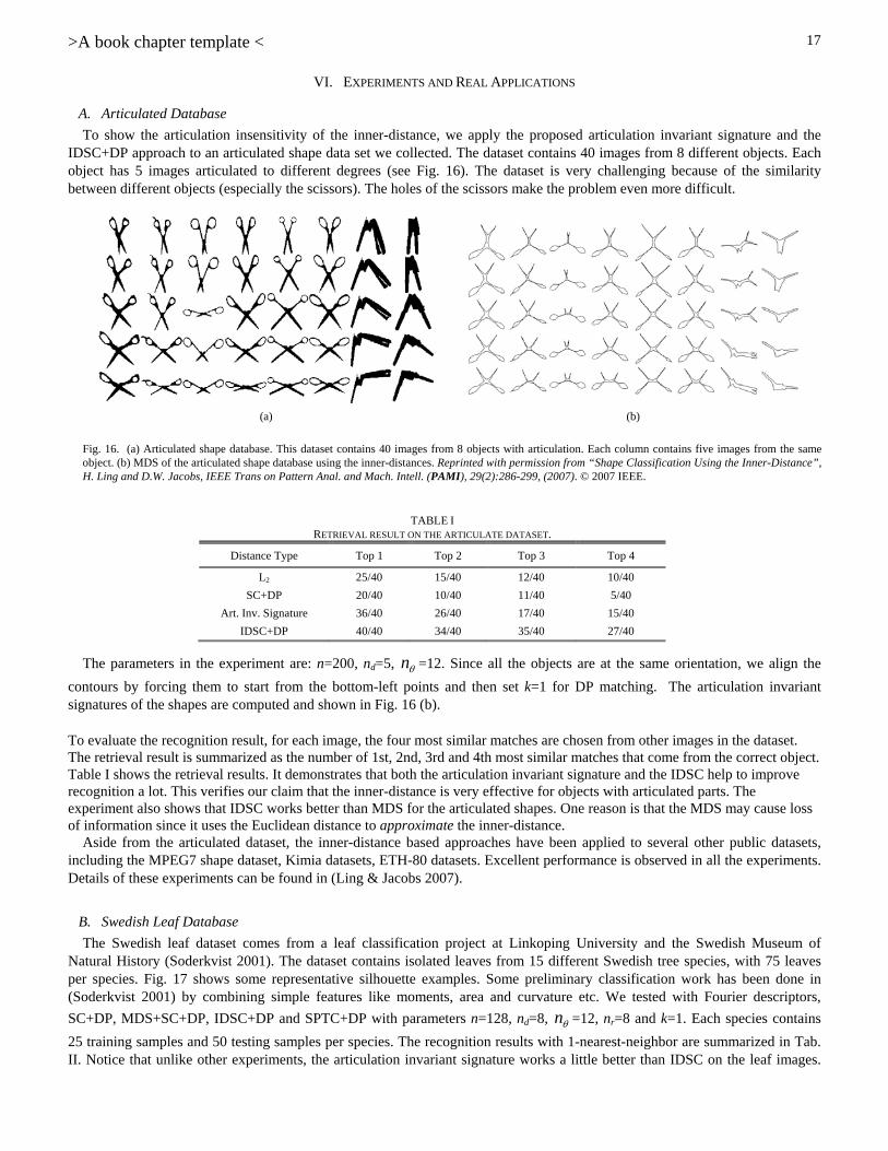
To show the articulation insensitivity of the inner-distance, we apply the proposed articulation invariant signature and the IDSC+DP approach to an articulated shape data set we collected. The dataset contains 40 images from 8 different objects. Each object has 5 images articulated to different degrees (see Fig. 16). The dataset is very challenging because of the similarity between different objects (especially the scissors). The holes of the scissors make the problem even more difficult.

The parameters in the experiment are: n=200, nd=5, n =12. Since all the objects are at the same orientation, we align the

contours by forcing them to start from the bottom-left points and then set k=1 for DP matching. The articulation invariant signatures of the shapes are computed and shown in Fig. 16 (b).

To evaluate the recognition result, for each image, the four most similar matches are chosen from other images in the dataset. The retrieval result is summarized as the number of 1st, 2nd, 3rd and 4th most similar matches that come from the correct object. Table I shows the retrieval results. It demonstrates that both the articulation invariant signature and the IDSC help to improve recognition a lot. This verifies our claim that the inner-distance is very effective for objects with articulated parts. The experiment also shows that IDSC works better than MDS for the articulated shapes. One reason is that the MDS may cause loss of information since it uses the Euclidean distance to approximate the inner-distance.

Aside from the articulated dataset, the inner-distance based approaches have been applied to several other public datasets, including the MPEG7 shape dataset, Kimia datasets, ETH-80 datasets. Excellent performance is observed in all the experiments. Details of these experiments can be found in (Ling & Jacobs 2007).

B. Swedish Leaf Database

The Swedish leaf dataset comes from a leaf classification project at Linkoping University and the Swedish Museum of Natural History (Soderkvist 2001). The dataset contains isolated leaves from 15 different Swedish tree species, with 75 leaves per species. Fig. 17 shows some representative silhouette examples. Some preliminary classification work has been done in (Soderkvist 2001) by combining simple features like moments, area and curvature etc. We tested with Fourier descriptors,

SC+DP, MDS+SC+DP, IDSC+DP and SPTC+DP with parameters n=128, nd=8, n =12, nr=8 and k=1. Each species contains

25 training samples and 50 testing samples per species. The recognition results with 1-nearest-neighbor are summarized in Tab. II. Notice that unlike other experiments, the articulation invariant signature works a little better than IDSC on the leaf images.

TABLE I RETRIEVAL RESULT ON THE ARTICULATE DATASET.

Distance Type Top 1 Top 2 Top 3 Top 4

L2 25/40 15/40 12/40 10/40

SC+DP 20/40 10/40 11/40 5/40

Art. Inv. Signature 36/40 26/40 17/40 15/40

IDSC+DP 40/40 34/40 35/40 27/40

(a) (b)

Fig. 16. (a) Articulated shape database. This dataset contains 40 images from 8 objects with articulation. Each column contains five images from the same object. (b) MDS of the articulated shape database using the inner-distances. Reprinted with permission from “Shape Classification Using the Inner-Distance”, H. Ling and D.W. Jacobs, IEEE Trans on Pattern Anal. and Mach. Intell. (PAMI), 29(2):286-299, (2007). © 2007 IEEE.


18

One possible explanation is that, as a real image dataset, the inner-angle for leaves are less robust due to boundary noise. Also notice that SPTC improves IDSC as we had expected.

C. Smithsonian Isolated Leaf Database

This data set comes from the Smithsonian project (Electronic Field Guide, 2008). We designed an Electronic Field Guide image retrieval system that allows online visual searching. The task is very challenging because it requires querying a database containing more than one hundred species and real time performance requires an efficient algorithm. In addition, the pictures taken in the field are vulnerable to lighting changes and the leaves may not be flattened well.

We evaluated the proposed approaches on a representative subset of the leaf image database in the system

(http://www.ist.temple.edu/~hbling/data/SI-93.zip). The subset contains 343 leaves from 93 species (the number of leaves from different species varies). In the experiment, 187 of them are used as the training set and 156 as the testing set. Note that there are only two instances per class in the training set on average. The retrieval performance is evaluated using performance curves which show the recognition rate among the top N leaves, where N varies from 1 to 16.

For the efficiency reasons mentioned above, only 64 contour points are used (i.e. n=64). The similarity between leaves is measured by the shape context distance Dsc (see Sec. II or (Belongie et al. 2002). This distance is based on a greedy matching and should not be confused with the bipartite matching based approach. Therefore it is faster than DP-based matching. Other

Fig. 18. The Smithsonian dataset. This dataset contains 343 leaf images from 93 species. Typical images from each species are shown. Reprinted with permission from “Shape Classification Using the Inner-Distance”, H. Ling and D.W. Jacobs, IEEE Trans on Pattern Anal. and Mach. Intell. (PAMI), 29(2):286-299, (2007). © 2007 IEEE.

TABLE II RECOGNITION RATES ON THE SWEDISH LEAF DATASET. NOTE THAT MDS+SC+DP AND SPTC ACHIEVED THE SAME RATES.

Method [SODERKVIST

2001] Fourier SC+DP MDS+SC+DP IDSC+DP SPTC+DP

Recognition Rate 82% 89.6% 8812.% 95.33% 94.13% 95.33%

Note that MDS+SC+DP and SPTC got same rates.

Fig. 17. Typical images from Swedish leaf data base, one image per species. Note that some species are quite similar, e.g. the 1st, 3rd and 9th species. Reprinted with permission from “Shape Classification Using the Inner-Distance”, H. Ling and D.W. Jacobs, IEEE Trans on Pattern Anal. and Mach. Intell. (PAMI), 29(2):286-299, (2007). © 2007 IEEE.


19

parameters used in the experiment are nd=5, n =12, and nr=8. Note that k is not needed because DP is not used here. The

performance is plotted in Fig. 19. It shows that SPTC works significantly better than other methods. Fig. 20 gives some detailed query results of SPTC and IDSC, from which we can see how SPTC improves retrieval result by also considering texture information.

VII. CONCLUSION

In this chapter, we present an inner-distance based shape matching algorithm for the application of foliage image retrieval. With experiments on two leaf databases involving thousands of images, our method demonstrates excellent performance in comparison to several state-of-the-art approaches. The approach is adopted in an electronic field guide system that has been tested in several real field test trips.

There are two main issues that are worth future study. First, the algorithm requires segmentation for preprocessing. In our current system images are taken by putting leaves against a white paper background. This is apparently not an ideal solution especially for use in the field. Second, more efficient schemes are needed for fast retrieval and browsing, especially for a large

Fig. 20. Three retrieval examples for IDSC and SPTC. The left column shows the query images. For each query image, the top four retrieving results are shown to its right, using IDSC and SPTC respectively. The circled images come from the same species as the query image. Reprinted with permission from “Shape Classification Using the Inner-Distance”, H. Ling and D.W. Jacobs, IEEE Trans on Pattern Anal. and Mach. Intell. (PAMI), 29(2):286-299, (2007). © 2007 IEEE.

Fig. 19. Recognition result on the Smithsonian leaf dataset. The ROC curves shows the recognition rate among the top N matched leaves. Reprinted with permission from “Shape Classification Using the Inner-Distance”, H. Ling and D.W. Jacobs, IEEE Trans on Pattern Anal. and Mach. Intell. (PAMI), 29(2):286-299, (2007). © 2007 IEEE.


20

database or an online system. One possibility is through smart indexing techniques instead of the currently used nearest neighbor algorithm. We look forward to future development in these directions.

ACKNOWLEDGMENT

We would like to thank J. W. Kress, R. Russell, N. Bourg, G. Agarwal, P. Belhumeur and N. Dixit for help with the Smithsonian leaf database, and O. Soderkvist for the Swedish leaf data. This work is supported in part by NSF (ITR-03258670325867) and by the US-Israel Binational Science Foundation grant number 2002/254.

REFERENCES Agarwal, S., Awan, A., & Roth, D. (2004). Learning to Detect Objects in Images via a Sparse, Part-Based Representation. IEEE Trans. on Pattern Analysis

and Machine Intelligence, 26(11), 1475-1490. Agarwal, G. (2005). Presenting Visual Information to the User : Combining Computer Vision and Interface Design. Master Thesis, Univseristy of Maryland,

2005. Agarwal, G., Belhumeur, P., Feiner, S., Jacobs, D., Kress, J. W., Ramamoorthi, R., Bourg, N., Dixit, N., Ling, H., Mahajan, D., Russell, R., Shirdhonkar, S.,

Sunkavalli, K., & White, S. (2006). First Steps Toward an Electronic Field Guide for Plants. Taxon, 55(3), 597-610. Basri, R., Costa, L., Geiger, D., & Jacobs, D. (1998). Determining the Similarity of Deformable Shapes. Vision Research, 38, 2365-2385. Bederson, B. B. (2001). PhotoMesa: A Zoomable Image Browser Using Quantum Treemaps and Bubblemaps. ACM Symposium on User Interface Software

and Technology, CHI Letters, 3(2), 71-80. Belongie, S., Malik, J., & Puzicha, J. (2002). Shape Matching and Object Recognition Using Shape Context. IEEE Trans. on Pattern Analysis and Machine

Intelligence, 24(24), 509-522. Biederman, I. (1987). Recognition--by--components: A theory of human image understanding. Psychological Review, 94(2), 115-147. Blum, H. (1973). Biological Shape and Visual Science. J. Theor. Biol., 38, 205-287. Bookstein, F. (1989). Principal Warps: Thin-Plate-Splines and Decomposition of Deformations. IEEE Trans. on Pattern Analysis and Machine Intelligence,

11(6), 567-585. Borg, I., & Groenen, P. (1997). Modern Multidimensional Scaling: Theory and Applications. Springer. Chen, H., Belhumeur, P., & Jacobs, D. (2000). In search of Illumination Invariants. IEEE Conf. on Computer Vision and Pattern Recognition, I, 254-261. Cormen, T., Leiserson, T, Rivest, R., & Stein, C. (2001). Introduction to Algorithms, the MIT Press, 2nd edition. Elad, A. & Kimmel, R. (2003). On Bending Invariant Signatures for Surfaces. IEEE Trans. on Pattern Analysis and Machine Intelligence, 25(10), 1285-1295. An Electronic Field Guide: Plant Exploration and Discovery in the 21st Century. (2008). Retrieved December 12, 2008, from

http://herbarium.cs.columbia.edu/. Feldman, J., & Singh, M. (2005). Information along contours and object boundaries. Psychological Review, 112(1), 243-252. Felzenszwalb, P. (2005). Representation and Detection of Deformable Shapes. IEEE Trans. on Pattern Analysis and Machine Intelligence, 27(2), 208-220. Felzenszwalb, P., & Huttenlocher, D. (2005). Pictorial Structures for Object Recognition, International Journal of Computer Vision, 61(1), 55-79. Felzenszwalb, P., & Schwartz, J. (2007). Hierarchical Matching of Deformable Shapes, IEEE Conference on Computer Vision and Pattern Recognition. Fergus, R., Perona, P., & Zisserman, A. (2003). Object Class Recognition by Unsupervised Scale-Invariant Learning, IEEE Conference on Computer Vision

and Pattern Recognition, II, 264-271. Gandhi, A. (2002). Content-based image retrieval: plant species identification, MS thesis, Oregon State University. Gorelick, L., Galun, M., Sharon, A., Basri, R., & Brandt, A. (2004), Shape Representation and Classification Using the Poisson Equation, IEEE Conference on

Computer Vision and Pattern Recognition, 61-67. Grenander, U., Srivastava, A., & Saini, S. (2007). A Pattern-Theoretic Characterization of Biological Growth, IEEE Transactions on Medical Imaging,

26(5):648-659. Grimson, W. E. L. (1990). Object Recognition by Computer: The Role of Geometric Constraints, MIT Press, Cambridge, MA. Hamza, A. B., & Krim, H. (2003). Geodesic Object Representation and Recognition. in I. Nystrom et al. (Eds.): Discrete Geometry for Computer Imagery,

LNCS, 2886, 378-387. Hoffman, D. D., & Richards, W. A. (1985). Parts of recognition, Cognition, 18, 65-96. Im, C., Nishida, H., & Kunii, T. L. (1998). Recognizing plant species by leaf shapes-a case study of the Acer family, International Conference on Pattern

Recognition, 2, 1171-1173. Keogh, E., Wei, L., Xi, X., Lee, S-H, & Vlachos, M. (2006). LB_Keogh Supports Exact Indexing of Shapes under Rotation Invariance with Arbitrary

Representations and Distance Measures. VLDB. Kimia, B. B., Tannenbaum, A. R., & Zucker S. W. (1995). Shapes, shocks, and deformations, I: The components of shape and the reaction-diffusion space,

International Journal of Computer Vision, 15(3), 189-224. Lazebnik, L., Schmid, C., & Ponce, J. (2005). A sparse texture representation using affine-invariant regions. IEEE Trans. Pattern Anal. Mach. Intell., 27(8),

1265-1278. Leibe, B., & Schiele, B. (2003). Analyzing Appearance and Contour Based Methods for Object Categorization, IEEE Conference on Computer Vision and

Pattern Recognition, II, 409-415. Ling, H., & Jacobs, D. W. (2005). Using the Inner-Distance for Classification of Articulated Shapes, IEEE Conference on Computer Vision and Pattern

Recognition II, 719-726. Ling, H., & Jacobs, D. W. (2005). Deformation Invariant Image Matching, IEEE International Conference on Computer Vision. II, 1466-1473, 2005. Ling, H. & Jacobs, D. W. (2007). Shape Classification Using the Inner-Distance, IEEE Trans on Pattern Anal. and Mach. Intell., 29(2), 286-299. Liu, T., & Geiger, D. (1997). Visual Deconstruction: Recognizing Articulated Objects, Energy Minimization Methods in Computer Vision and Pattern

Recognition, 295-309. Mikolajczyk, K., & Schmid, C. (2005). A Performance Evaluation of Local Descriptors. IEEE Trans. Pattern Anal. Mach. Intell., 27(10):1615-1630. Mokhtarian, F., & Abbasi, S. (2004). Matching shapes with self-intersections: application to leaf classification. IEEE Trans. on Image Processing, 13(5), 653-

661. Mori, G., & Malik, J. (2003). Recognizing Objects in Adversarial Clutter: Breaking a Visual CAPTCHA, IEEE Conference on Computer Vision and Pattern

Recognition, I, 1063-6919. Nilsback, M., & Zisserman, A. (2006). A Visual Vocabulary for Flower Classification. IEEE Conf. on Computer Vision and Pattern Recognition, 2:1447-

1454.


21

Osada, R., Funkhouser, T., Chazelle, B., & Dobkin, D. (2002). Shape Distributions, ACM Trans. on Graphics, 21(4), 807-832. Petrakis, E. G. M., Diplaros, A., & Milios, E. (2002). Matching and Retrieval of Distorted and Occluded Shapes Using Dynamic Programming, IEEE Trans.

on Pattern Analysis and Machine Intelligence, 24(11), 1501-1516. Saitoh, T., & Kaneko, T. (2000). Automatic Recognition of Wild Flowers, International Conference on Pattern Recognition, 2, 2507-2510. Sclaroff, S., & Liu, L. (2001). Deformable shape detection and description via model-based region grouping, IEEE Trans. on Pattern Analysis and Machine

Intelligence, 23(5), 475-489. Schneiderman, H., & Kanade, T. (2004). Object Detection Using the Statistics of Parts, International Journal of Computer Vision, 56(3), 151-177. Sebastian, T. B., Klein, P. N., & Kimia, B. B. (2004). Recognition of Shapes by Editing Their Shock Graphs, IEEE Trans. on Pattern Analysis and Machine

Intelligence, 26(5), 550-571. Siddiqi, K, Shokoufandeh, A., Dickinson, S. J., & Zucker, S. W. (1999). Shock Graphs and Shape Matching, International Journal of Computer Vision, 35(1),

13-32. Soderkvist, O. (2001). Computer Vision Classification of Leaves from Swedish Trees, Master Thesis, Linkoping University. Thayananthan, A., Stenger, B., Torr, P. H. S., & Cipolla, R. (2003). Shape Context and Chamfer Matching in Cluttered Scenes, IEEE Conference on Computer

Vision and Pattern Recognition, I, 127-133. Thompson, D. W. (1992) On Growth and Form. (republished), Dover Publication. Tu, Z., & Yuille, A. L. (2004). Shape Matching and Recognition-Using Generative Models and Informative Features, European Conference on Computer

Vision, 3, 195-209. Veltkamp, R. C., & Hagedoorn, M. (1999). State of the Art in Shape Matching, Technical Report UU-CS-1999-27, Utrecht. Wang, Z., Chi, Z., & Feng, D. (2003). Shape based leaf image retrieval, IEE proc. Vision, Image and Signal Processing, 150(1), 34-43. Weiss, I., & Ray, M. (2005). Recognizing Articulated Objects Using a Region-Based Invariant Transform, IEEE Trans. on Pattern Analysis and Machine

Intelligence, 27(10), 1660- 1665. Yahiaoui, I., Herve, N., & Boujemaa, N. (2005). Shape-based image retrieval in botanical collections. Zhao, L., & Davis, L. S. (2005). Segmentation and Appearance Model Building from an Image Sequence, IEEE International Conference on Image

Processing, 1, 321-324.

shape matching for foliage database retrievalhbling/publication/foloiage_igi_5.pdf · leaves (see...

Documents