shape preserving local histogram modification - image ...vcaselles/papers_v/shapelhisto.pdf · 220...

220 IEEE TRANSACTIONS ON IMAGE PROCESSING, VOL. 8, NO. 2, FEBRUARY 1999

Shape Preserving Local Histogram ModificationVicent Caselles,Associate Member, IEEE,Jose-Luis Lisani, Jean-Michel Morel, and Guillermo Sapiro,Member, IEEE

Abstract—A novel approach for shape preserving contrastenhancement is presented in this paper. Contrast enhancementis achieved by means of alocal histogram equalization algorithmwhich preserves thelevel-setsof the image. This basic property isviolated by common local schemes, thereby introducing spuriousobjects and modifying the image information. The scheme isbased on equalizing the histogram in all theconnected componentsof the image, which are defined based both on the grey-valuesand spatial relations between pixels in the image, and followingmathematical morphology, constitute the basic objects in thescene. We give examples for both grey-value and color images.

Index Terms—Connected components, histogram equalization,level-sets, local operations, mathematical morphology.

I. INTRODUCTION

I MAGES ARE captured at low contrast in a number ofdifferent scenarios. The main reason for this problem is

poor lighting conditions (e.g., pictures taken at night or againstthe sun rays). As a result, the image is too dark or toobright, and is inappropriate for visual inspection or simpleobservation. The most common way to improve the contrast ofan image is to modify its pixel value distribution, orhistogram.A schematic example of the contrast enhancement problem andits solution via histogram modification is given in Fig. 1. Onthe left, we see a low contrast image with two different squares,one inside the other, and its corresponding histogram. We canobserve that the image has low contrast, and the differentobjects cannot be identified, since the two regions have almostidentical grey values. On the right we see what happens whenwe modify the histogram in such a way that the grey valuescorresponding to the two regions are separated. The contrastis improved immediately.

Histogram modification, and in particular histogram equal-ization (uniform distributions), is one of the basic and mostuseful operations in image processing, and its description canbe found in any book on image processing. This operation is a

Manuscript received March 27, 1997; revised April 28, 1998. This workwas supported in part by DGICYT Project under Reference PB94-1174, bythe Math, Computer, and Information Sciences Division, Office of NavalResearch under Grant ONR-N00014-97-1-0509, by NSF-LIS, and by theONR Young Investigator Program.

V. Caselles and J.-L. Lisani are with the Department of Mathematics andInformatics, University of Illes Balears, 07071 Palma de Mallorca, Spain(e-mail: [email protected]).

J.-M. Morel is with the Department of Applied Mathematics, EcoleNormale Superieure Cachan, 94235 Cachan Cedex, France (e-mail: [email protected]).

G. Sapiro is with the Department of Electrical and Computer Engi-neering, University of Minnesota, Minneapolis, MN 55455 USA (e-mail:[email protected]).

Publisher Item Identifier S 1057-7149(99)00936-7.

Fig. 1. Schematic explanation of the use of histogram modification toimprove image contrast.

particular case of homomorphic transformations: Letbe the image domain and: the given (lowcontrast) image. Let : be a given functionwhich we assume to be increasing. The image iscalled ahomomorphic transformationof . The particular caseof histogram equalization corresponds to selectingto be thedistribution function of :

AreaArea

(1)

If we assume that is strictly increasing, then the changeof variables

(2)

gives a new image whose distribution function is uniform inthe interval , , . This useful and basicoperation has an important property which, in spite of beingobvious, we would like to acknowledge: it neither creates nordestroys image information.

As argued by themathematical morphologyschool [1], [6],[7], the basic operations on images should be invariant withrespect to contrast changes, i.e., homomorphic transformations.As a consequence, it follows that the basic information of animage is contained in the family of its binary shadows orlevel-sets,that is, in the family of sets

(3)

for all values of in the range of . Observe that, under fairlygeneral conditions, an image can be reconstructed from itslevel-sets by the formula . If is astrictly increasing function, the transformation doesnot modify the family of level-sets of , it only changes itsindex in the sense that

for all (4)

1057–7149/99$10.00 1999 IEEE

CASELLES et al.: LOCAL HISTOGRAM MODIFICATION 221

Although one can argue ifall operations in image processingmust hold this principle, for the purposes of the present paperwe shall stick here to this basic principle. There are a numberof reasons for this. First of all, a considerable large amountof the research in image processing is based on assuming thatregions with (almost) equal grey-values, which are topolog-ically connected (see below), belong to the same physicalobject in the three-dimensional (3-D) world. Following this,it is natural to assume then that the “shapes” in an givenimage are represented by its level-sets (we will later see howwe deal with noise that produces deviations from the level-sets). Furthermore, this commonly assumed image processingprinciple will permit us to develop a theoretical and practicalframework for shape preserving contrast enhancement. Thiscan be extended to other definitions of shape, different from thelevel-sets morphological approach here assumed. We shouldnote that the level-sets theory is also applicable to a largenumber of problems beyond image processing [5], [10].

In this paper, we want to designlocal histogram modi-fication operations that preserve the family of level-sets ofthe image, that is, following the morphology school, preserveshape. Local contrast enhancement is mainly used to furtherimprove the image contrast and facilitate the visual inspectionof the data. As we will see later in this paper, global histogrammodification does not always produce good contrast; smallregions, especially, are hardly visible after such a globaloperation. On the other hand, local histogram modificationimproves the contrast of small regions as well, but since thelevel-sets are not preserved, artificial objects are created. Thetheory developed in this paper will enjoy the best of bothwords: the shape-preservation property of global techniquesand the contrast improvement quality of local ones.

The recent formalization of multiscale analysis given in [1]leads to a formulation of recursive, causal, local, morpholog-ical, and geometric invariant filters in terms of solutions ofcertain partial differential equations of geometric type, provid-ing a new view on many of the basic mathematical morphologyoperations. One of their basic assumptions was the localityassumption, which aimed to translate into a mathematicallanguage the fact that we considered basic operations whichwere a kind of local average around each pixel or, in otherwords, only a few pixels around a given sample influencethe output value of the operations. Obviously, this excludedthe case of algorithms as histogram modification. This is whyoperations like those in [8] and [9] and the one described inthis paper are not modeled by these equations, and a novelframework must be developed.

It is not the goal of this paper to review the extensiveresearch performed in contrast enhancement. We should onlynote that basically, contrast enhancement techniques are di-vided in the two groups mentioned above, local and global,and their most popular representatives can be found in anybasic book in image processing and computer vision. An earlyattempt to introduce shape criteria in contrast enhancementwas done in [3]. To the best of our knowledge, none of thevariations to histogram modification reported in the literaturehave formally approached the problem of shape preservingcontrast enhancement as done in this paper.

II. GLOBAL HISTOGRAM MODIFICATION:A VARIATIONAL FORMULATION

We call representativesof all images of the form, where is a strictly increasing function. The question

is, which representative of is the best for our purposes? Thatwill depend, of course, in what our purposes are. We have seenabove which is the function we have to select if we wantto normalize the contrast making the distribution function of

uniform. In addition, it was shown in [8] and [9] that whenequalizing an image: on the range we areminimizing the functional

(5)

The second term of the integral can be understood as ameasure of the contrast of the whole image. Thus, whenminimizing we are distributing the values ofso that wemaximize the contrast. The first term tries to keep the values of

as near as possible to the mean . When minimizingon the class of functions with the same family of binary

shadows as , we get the equalization of. We will see belowhow to modify this energy to obtain shape preserving localcontrast enhancement.

III. CONNECTED COMPONENTS

To be able to extend the global approach to a local setting,we have to insist in our main constraint: we have to keepthe same topographic map, that is, we have to keep the samefamily of level-sets of but we have the freedom to assignthem a “convenient” grey level. To make this statement moreprecise, let us give some definitions (see [11]).

Definition 1: Let be a topological space. We say thatis connected if it cannot be written as the union of two

nonempty closed (open) disjointsets. A subsetof is calleda connected component if is a maximal connected subsetof , i.e., is connected and for any connected subsetof

such that , then .This definition will be applied to subsets of which

are topological spaces with the topology induced from,i.e., an open set of is the intersection of an open set of

with . We shall need the following observation whichfollows from the definition above: Two connected componentsof a topological space are either disjoint or they coincide; thus,the topological space can be considered as the disjoint unionof its connected components.

Remark: There are several notions of connectivity for atopological space. One of the most intuitive ones is thenotion of arcwise connected (also called connected by arcs).A topological space is said to be connected by arcs if anytwo points of can be joined by an arc, i.e., there existsa continuous function : such that ,

. In a similar way as above we define the connectedcomponents (with respect to this notion of connectivity) as themaximal connected sets. These notions could be used belowinstead of the one given in Definition 1.


Definition 2: Let : be a given image and ,, . A section of the topographic map of

is a set of the form

(6)

where is a connected component of such that foreach , , , the set

(7)

is also connected.Definition 3: Let : be a given image and let

: be the family of its level-sets. We shall saythat the mapping : is a local contrast changeif the following properties hold.

P1: is continuous in the following sense:

when

being a connected component of .P2: is an increasing function of for all .P3: for all , are in the same

connected component of , .P4: Let be a connected set with not reduced to

a point. Let . Then is notreduced to a point.

P5: Let be a section of thetopographic map of , , and let ,

. Then .

Definition 4: Let : be a given image. We shallsay that is a local representative of if there exists somelocal contrast change such that , .

We collect in the next proposition some properties whichfollow immediately from the definitions above.

Proposition 1: Let : and let, , be a local representative of. Then,

we have the following.

1) : . We have thatif and only if , , .

2) is a continuous function.3) Let ( ) be a connected component of (resp.

) containing , . Then .4) Let be a section of the topographic map of.

Then is also a section of the topographic mapof .

Proof:

1) Is a simple consequence ofP2 in Definition 3.2) Is a consequence ofP1 in Definition 3.3) By P3 of Definition 3, we have . Since

and is connected, then . Now, supposethat

Thus, is not reduced to a point. ByP4 of Definition3, is not reduced to a point, a contradiction since

on . It follows that . Since isconnected and , then .

4) Let be a section of the topo-graphic map of . Let and . ByPart 3, coincides with the connected component of

containing which we denote by .Let , . Since, usingP5, :

, then we may write. Now it is easy to see that is a

section of the topographic map of.

Remarks:

1) The previous proposition can be phrased as saying thatthe set of “objects” contained in is the same as theset of “objects” contained in , if we understand the“objects” of as the connected components of the level-sets , , and, respectively, for .

2) Our definition of local representative is contained in thenotion of dilation as given in [6] and [7], Th. 9.3. Let

be a lattice of functions : . A mapping: is called a dilation of if and only if it

can be written as

where is a function assigned to each pointand is possibly different from point

to point. Thus, let be a local contrast change and let. Let us denote by the con-

nected component of which contains if ,otherwise, let . Letif ; and if

. Then .3) Extending the definition of local contrast change to

include more general functions than continuous ones,i.e., to include measurable functions, we can state andprove a converse of Proposition 1, saying that thetopographic map contains all the information of theimage which is invariant by local contrast changes [2].

IV. SHAPE PRESERVING CONTRAST ENHANCEMENT

We can now state precisely the main question we want toaddress:what is the best local representativeof , when thegoal is to perform local contrast enhancement while preservingthe connected components (and level-sets). For that we shalluse the energy formulation given in Section II. Let be aconnected component of the set , , ,

. Write

(8)

We then look for a local representativeof that minimizesfor all connected components of all sets of the

form , , , , or, in other words,


the distribution function of in all connected components ofis uniform in the range , for all , ,

. We now show how to solve this problem.Let us introduce some notation that will make our discussion

easier. Without loss of generality we assume that:. Let , , .

We need to assume that, the distribution function of , iscontinuous and strictly increasing. For that we assume thatis continuous and1

Area for all (9)

We shall construct a sequence of functions convergingto the solution of the problem. Let be thehistogram equalization of . Suppose that we already con-structed . Let us construct . For each

, let

(10)

and let be the connected components of ,( can be eventually ). Define

(11)

By our assumption (9), is a continuous strictlyincreasing function in , and we can equalize thehistogram of in . Thus, we define

(12)

and

(13)

We will then prove the following.Theorem 1: Under the assumption (9), the functions

have a uniform histogram for all connected components of all“dyadic” sets of the form where , :

, . Moreover, as , convergesto a function that has a uniform histogram for all connectedcomponents of all sets , for all , ,

.Theorem 2: Let be the function constructed in Theorem

1. Then is a local representative of.The proof of Theorem 1 is based in the next two simple

lemmas.Lemma 1: Let , such that . Let: , , be two functions with uniform

histogram in . Let : be given by

if ,

if .(14)

Then, has a uniform histogram in .

1This assumption is mainly theoretical and does not necessarily need tohold for basic practical purposes.

Lemma 2: Let , such that . Let :, : be two functions with uniform

histogram in , , respectively. Assume that

(15)

Let : be given by

if ,

if .(16)

Then has a uniform histogram in .Proof of Theorem 1:The first part of the statement fol-

lows immediately from the two lemmas above. Now, considerthe sequence . Observe that

for all (17)

Indeed, if , , then ,, while, if , then

, . The estimate (17) follows.Now, since

(18)

and the series on the right-hand side is absolutely convergent,then converges absolutely and uniformly to some contin-uous function : . satisfies the statement above.Indeed, since

for all (19)

and is the uniform limit of , then for all there issome such that

(20)

for all , and all . Letting, it follows that

for all (21)

If is not dyadic, let , be such that. Then

(22)Thus, by approaching with dyadic numbers, we prove that

for all (23)

Let us mention in passing that the above proof also shows that

Area for all (24)

Similarly, one proves that has a uniform histogram in allconnected components of all sets of the form forall dyadic numbers , , . Now let ,and let be a connected component of . Let

, be such that . Let be


a connected component of containing .Then

(25)

for all . By property (24), we may approachandby dyadic numbers while . It follows that

(26)

The other inequality is proved in a similar way. It follows thathas a uniform histogram for all connected components of

all sets of the form for all numbers , ,.

Proof of Theorem 2:We shall use the notation intro-duced previously. First we define ( beingthe global histogram of ). Let . Let , .Let be such that . Then we define

if ,if ,if .

It is clear that is a local contrast change of. Let us checkthat is a local contrast change of , , i.e., it satisfiesP1–P5, for all . To simplify our notation, let us writeinstead of .

P1 : Let , , , .Suppose that , and .Then either or for some. If , then ,

and . Hence, and, , . Then

. If , then one easily checksthat .

P2 : Follows from the definition of .P3 : Let , be in the same connected component of

, . Let be such that ,. Then, for some . Then

.P4 : Let be a connected set with not re-

duced to a point. Let . Since, for some , is not

reduced to a point. Thus, there existwith . Then,

. Theset : is not reduced to a point.

P5 : Let be a section of thetopographic map of and let , .Let be such that , , .If , , thensince is connected and contains. Thus,

. Hence,. Let , be such that

, , . Then.

Let , ,. Observe that . Since

(27)

and

the series in (27) is absolutely and uniformly convergent.Hence, for some function .It follows that . Let us now prove that

is a local contrast change for.

P1: Let , , , . Since

(28)

then

(29)

Using the corresponding propertyH1 we see thatas , .

P2: Follows from P2 and the definition of .P3: Let , be in the same connected component of

, . Thenand , are in the same connected component of

. Then .Proceeding iteratively and usingP3 we get that

for all . Lettingwe get that .

P4: Let be a connected set with not reducedto a point. For any , let be theconnected component of containing .Let . Since is not reducedto a point, it contains an interval. This implies thatArea . Now we observe that .Obviously, . Now, let forsome . Since, byP3, , we havethat . It follows that ,hence the equality. If was reduced to a point

, then . Hence, AreaArea , contradicting (24). Thereforecannot be reduced to a point.

P5: Let be a section of thetopographic map of and let , . First,usingP5 and the fact that each transformsinto a section of the topographic map of (Proposi-tion 1), it follows that forall . Letting , we get that

. Now, let . Since ,are also sections of the topographic map

of , then by the previous observation we have. If

, then for all


Fig. 2. Example of the level-sets preservation. The top row shows the original image and its level-sets. The second row shows the result of globalhistogram modification and the corresponding level-sets. Results of classical local contrast enhancement and its corresponding level-sets are shown inthe third row. The last row shows the result of our algorithm. Note how the level-sets are preserved, in contrast with the result on the third row, whilethe contrast is much better than the global modification.

and some constant. Hence AreaArea , again a contradiction with

(24). Thus, .

Proof of Lemma 1:Let . Since

it follows that

Hence, has a uniform histogram.

Proof of Lemma 2:Let . Since

Now, let . Since

We conclude that has a uniform histogram.


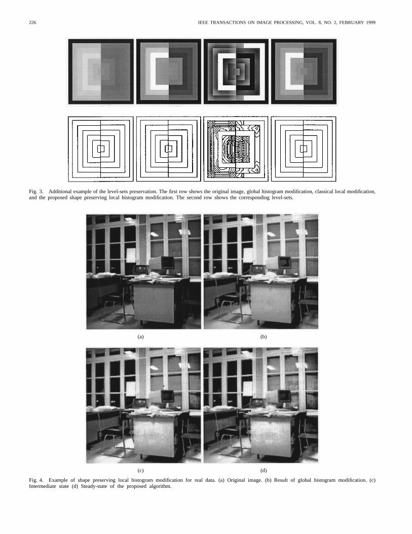
Fig. 3. Additional example of the level-sets preservation. The first row shows the original image, global histogram modification, classical local modification,and the proposed shape preserving local histogram modification. The second row shows the corresponding level-sets.

(a) (b)

(c) (d)

Fig. 4. Example of shape preserving local histogram modification for real data. (a) Original image. (b) Result of global histogram modification. (c)Intermediate state (d) Steady-state of the proposed algorithm.


(a) (b)

(c) (d)

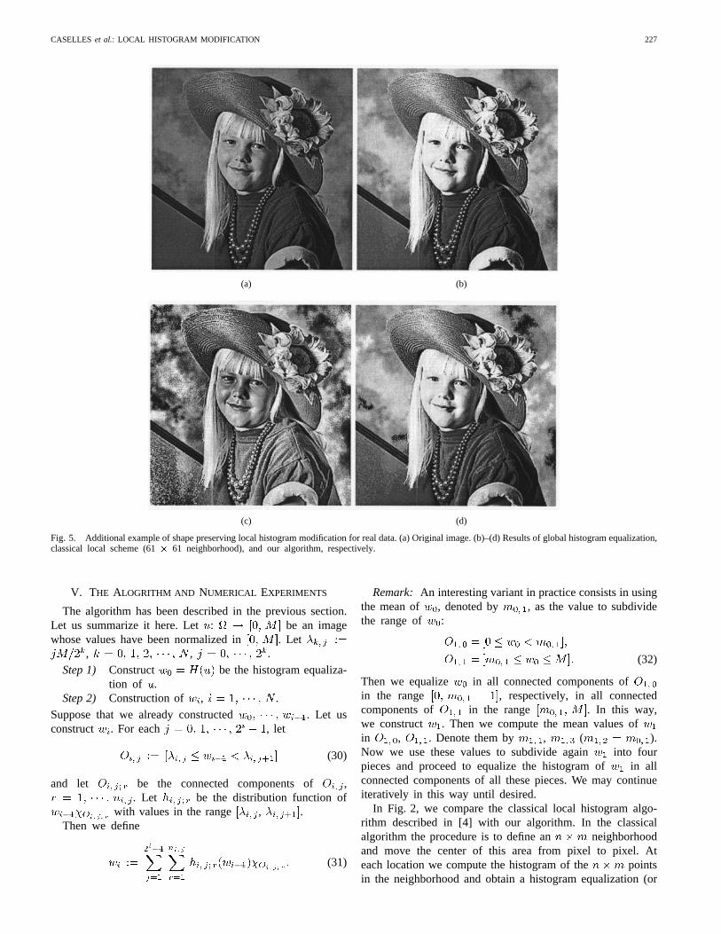
Fig. 5. Additional example of shape preserving local histogram modification for real data. (a) Original image. (b)–(d) Results of global histogram equalization,classical local scheme (61� 61 neighborhood), and our algorithm, respectively.

V. THE ALOGRITHM AND NUMERICAL EXPERIMENTS

The algorithm has been described in the previous section.Let us summarize it here. Let: be an imagewhose values have been normalized in . Let

, , .

Step 1) Construct be the histogram equaliza-tion of .

Step 2) Construction of , .

Suppose that we already constructed . Let usconstruct . For each , let

(30)

and let be the connected components of ,. Let be the distribution function of

with values in the range , .Then we define

(31)

Remark: An interesting variant in practice consists in usingthe mean of , denoted by , as the value to subdividethe range of :

(32)

Then we equalize in all connected components ofin the range , respectively, in all connectedcomponents of in the range . In this way,we construct . Then we compute the mean values ofin , . Denote them by , ( ).Now we use these values to subdivide again into fourpieces and proceed to equalize the histogram ofin allconnected components of all these pieces. We may continueiteratively in this way until desired.

In Fig. 2, we compare the classical local histogram algo-rithm described in [4] with our algorithm. In the classicalalgorithm the procedure is to define an neighborhoodand move the center of this area from pixel to pixel. Ateach location we compute the histogram of the pointsin the neighborhood and obtain a histogram equalization (or


Fig. 6. Example of local histogram modification of a color image. The original image is shown on the top. The bottom left is the result of applying ouralgorithm to the Y channel in the YIQ color space. On the right, the algorithm is applied again only to the Y channel, but rescaling the chrominancevector to maintain the same color point on the Maxwell triangle.

(a) (b) (c)

Fig. 7. Comparison between the classical local histogram modification scheme with the new one proposed in this paper for a color image. (a) Original image.(b) Image obtained with the classical technique. (c) Result of applying our scheme. Note the spurious objects introduced by the classical local scheme.

histogram specification) transformation function. This functionis used to map the level of the pixel centered in the neigh-borhood. The center of the region is then moved toan adjacent pixel location and the procedure is repeated. Inpractice, one updates the histogram obtained in the previouslocation with the new data introduced at each motion step.Fig. 2(a) shows the original image whose level-lines aredisplayed in Fig. 2(b). In Fig. 2(c) we show the result ofthe global histogram equalization of Fig. 2(a). Its level-linesare displayed in Fig. 2(d). Note how the level-sets lines arepreserved, while the contrast of small objects is reduced.Fig. 2(e) shows the result of the classical local histogramequalization described above (31 31 neighborhood), withlevel-lines displayed in Fig. 2(f).2 We see that new level-lines appear thus modifying the topographic map (the set oflevel-lines) of the original image, introducing new objects.Fig. 2(g) shows the result of our algorithm for local histogram

2All the level sets for grey-level images are displayed at intervals of 20grey-values.

equalization. Its corresponding level-lines are displayed inFig. 2(h). We see that they coincide with the level-lines ofthe original image, Fig. 2(b).

Fig. 3 repeats the experiments in Fig. 2 for another syntheticimage. Fig. 3(a) has been constructed by cutting half of theright side of Fig. 2(a) and putting it at the left side of it.Fig. 3(b) shows the global histogram equalization of Fig. 3(a).Fig. 3(c) shows the result of the classical local histogramequalization described above. Fig. 3(d) presents the result ofour algorithm applied to Fig. 3(a). The level-lines off all thefigures are given in Fig. 3(e)–(h), respectively. We see howdifferent connected components do not interact in the proposedscheme, and the contrast is improved while preserving theobjects in the scene.

Results for a real image are presented in Fig. 4. Fig. 4(a)is the typical “Bureau de l’INRIA” image. Fig. 4(b) is theglobal histogram equalization of Fig. 4(a). Fig. 4(c) shows anintermediate step of the proposed algorithm, while Fig. 4(d) isthe steady-state solution. Note how objects that are not visible


in the global modification, like those through the window, arenow visible with the new local scheme.

An additional example is given in Fig. 5. Fig. 5(a) isthe original image. Fig. 5(b)–(d) are the results of globalhistogram equalization, classical local scheme (6161 neigh-borhood), and our algorithm, respectively.

Experiments with a color image are given in Fig. 6, workingon the YIQ (luminance and chrominance) color space. InFig. 6(a) we present the original image. In Fig. 6(b), ouralgorithm has been applied to the luminance image Y (main-taining IQ) and then we recomposed the RGB color system.In Fig. 6(c), again, we apply the proposed local histogrammodification to the color Y channel only, but rescaling thechrominance vector to maintain the same color point on theMaxwell triangle.

In the last example, Fig. 7, we compare the classical localhistogram modification scheme with the new one proposed inthis paper for a color image, following the same procedure asin Fig. 6. Fig. 7(a) shows the original image, Fig. 7(b) the oneobtained with the classical technique, and Fig. 7(c) the resultof applying our scheme. Note the spurious objects introducedby the classical local scheme. (This figure is reproduced inblack and white here.)

VI. CONCLUDING REMARKS

This paper presented a novel algorithm for the most basicand (probably) most important operation in image processing:contrast enhancement. The algorithm is motivated by ideasfrom the mathematical morphology school, and it holds themain properties of both global and local schemes: It preservesthe level-sets of the image, that is, its basic morphologicalstructure, as global histogram modification does, while achiev-ing high contrast results as in local histogram modifications.

A number of problems remain open in this area, and webelieve they can be approached with the framework presentedin this paper, which complements the results in [8] and [9].One of the open problems is to extend the algorithm to otherdefinitions of connected components, that is, other definitionsof objects. In this paper, we define objects as done by themathematical morphology school, via level-sets, and since thisis not the only possible definition, it remains to be shownthat a similar approach can be used for other relevant objectdescriptions. Note that objects can be defined also via opticalflow components in video data, or with a concept of connectedcomponents in multivalued images. A general framework forshape preserving contrast enhancement should include thesepossible definitions as well.

From the energy formulation shown in this paper, (5), it isclear that histogram modification is using a measurement ofcontrast that it is not appropriate at least for human vision. Thisis because absolute value is not a good model for how humansmeasure contrast (this value should be at least normalized bythe average brightness of the pixel region). The extension ofthe approach presented in this paper to other models of imagecontrast is an interesting open area as well. We expect toaddress these issues elsewhere.

ACKNOWLEDGMENT

The authors wish to thank INRIA for the use of theirdatabase.

REFERENCES

[1] L. Alvarez, F. Guichard, P. L. Lions, and J. M. Morel, “Axioms andfundamental equations of image processing,”Arch. Rational Mechan.Anal., vol. 16, pp. 200–257, 1993.

[2] V. Caselles, J. L. Lisani, J. M. Morel, and G. Sapiro, “The informationof an image invariant by local contrast changes,” 1998, preprint.

[3] R. Cromartie and S. M. Pizer, “Edge-affected context for adaptivecontrast enhancement,” inProc. Information Processing in MedicalImaging, Lecture Notes in Comp. Science,Wye, U.K., July 1991, vol.511, pp. 474–485.

[4] R. C. Gonzalez and P. Wintz,Digital Image Processing. Reading, MA:Addison-Wesley, 1987.

[5] S. J. Osher and J. A. Sethian, “Fronts propagation with curvaturedependent speed: Algorithms based on Hamilton–Jacobi formulations,”J. Comput. Phys.,vol. 79, pp. 12–49, 1988.

[6] J. Serra,Image Analysis and Mathematical Morphology.New York:Academic, 1982.

[7] , Image Analysis and Mathematical Morphology, Vol. 2: Theoret-ical Advances. New York: Academic, 1988.

[8] G. Sapiro and V. Caselles, “Histogram modification via differentialequations,”J. Differential Equat.,vol. 135, pp. 238–268, 1997.

[9] , “Contrast enhancement via image evolution flows,”Graph.Models Image Process.,vol. 59, pp. 407–416, 1997.

[10] J. A. Sethian,Level Set Methods: Evolving Interfaces in Geometry, FluidMechanics, Computer Vision and Materials Sciences.Cambridge,U.K.: Cambridge Univ. Press, 1996.

[11] L. Schwartz,Analyze I: Theorie des Ensembles et Topologie.Paris,France: Hermann, 1991.

Vicent Caselles(M’95–A’96) received the Licen-ciatura and Ph.D. degrees in mathematics fromValencia University, Spain, in 1982 and 1985, re-spectively.

Currently, he is an Associate Professor at the Uni-versity of Illes Balears, Palma de Mallorca, Spain.His research interests include image processing,computer vision, and the applications of geometryand partial differential equations to both previousfields.

Dr. Caselles was guest co-editor of the IEEETRANSACTIONS ON IMAGE PROCESSING special issue on partial differentialequations and geometry-driven diffusion in image processing and analysis(March 1998).

Jose-Luis Lisani was born in 1970. He receivedthe diploma from the Escuela Tecnica Superiorde Ingenieros de Telecomunicacion de Barcelona(ETSETB-Spain), Palma de Mallorca, Spain, intelecommunication engineering in 1995.

He is currently a Ph.D. student at Ceremade,University, Paris Dauphine, France. His previousresearch was at the Universitat de les Illes Balears(UIB-Spain), advised by V. Caselles (UIB),concerning the segmentation of 3-D images byminimizing the Mumford–Shah functional. From

1995 to 1997, he worked at the UIB in several European Union projects,including NEMESIS and CHARM. His research fields are mathematicalmorphology applied to comparison of images, and optical flow estimation.


Jean-Michel Morel received the Ph.D. degree inapplied mathematics and the Doctorat d’Etat, bothfrom the University Pierre et Marie Curie, France,in 1980 and 1985, respectively.

He is currently a Professor of applied mathemat-ics at the Ecole Normale Superieure de Cachan,Cachan, France. He has been working on the math-ematical formalization of image analysis problemssince 1988, and is co-author (with S. Solimini) ofa book on variational methods in image segmenta-tion.

Dr. Morel was guest co-editor of the IEEE TRANSACTIONS ON IMAGE

PROCESSINGspecial issue on partial differential equations and geometry-drivendiffusion in image processing and analysis (March 1998).

Guillermo Sapiro (M’95) was born in Montevideo,Uruguay, on April 3, 1966. He received the B.Sc.(summa cum laude), M.Sc., and Ph.D. degrees fromthe Department of Electrical Engineering, Tech-nion—Israel Institute of Technology, Haifa, in 1989,1991, and 1993, respectively.

After conducting post-doctoral research at theMassachusetts Institute of Technology, Cambridge,he became a Member of Technical Staff at theresearch facilities of Hewlett-Packard Laboratories,Palo Alto, CA. He is currently with the Department

of Electrical and Computer Engineering, University of Minnesota, Minneapo-lis. He works on differential geometry and geometric partial differentialequations, both in theory and applications in computer vision and imageanalysis.

Dr. Sapiro was guest co-editor of the IEEE TRANSACTIONS ON IMAGE

PROCESSINGspecial issue on partial differential equations and geometry-drivendiffusion in image processing and analysis (March 1998). He was awardedthe Gutwirth Scholarship for Special Excellence in Graduate Studies in 1991,the Ollendorff Fellowship for Excellence in Vision and Image UnderstandingWork in 1992, the Rothschild Fellowship for Post-Doctoral Studies in 1993,and the ONR Young Investigator Award in 1998.

shape preserving local histogram modification - image ...vcaselles/papers_v/shapelhisto.pdf · 220...

Documents