shape-similarity search of three-dimensional models using

Accepted for publication in the proceedings of the Pacific Graphics 2002, Beijing, China, October 9-11, 2002.

1/10

Shape-Similarity Search of Three-Dimensional Models

Using Parameterized Statistics

1Ryutarou Ohbuchi, 1Tomo Otagiri, 2Masatoshi Ibato, 1Tsuyoshi Takei

[email protected], [email protected] , [email protected], [email protected] 1 Computer Science Department, Yamanashi University, 4-3-11 Takeda, Yamanashi-shi, Japan

2 Ibaraki Computing Center, Incorporated.

Abstract

In this paper, we propose a method for shape-similarity

search of 3D polygonal-mesh models. The system accepts

triangular meshes, but tolerates degenerated polygons,

disconnected component, and other anomalies. As the

feature vector, the method uses a combination of three

vectors, (1) the moment of inertia, (2) the average distance

of surface from the axis, and (3) the variance of distance of

the surface from the axis. Values in each vector are

discretely parameterized along each of the three principal

axes of inertia of the model. We employed the Euclidean

distance and the elastic-matching distance as the measures

of distance between pairs of feature vectors. Experiments

showed that the proposed shape features and distance

measures perform fairly well in retrieving models having

similar shape from a database of VRML models.

Keywords: content-based search and retrieval, geometric

modeling, polygonal mesh, principal axes, elastic matching.

1. Introduction

With the recent increase in the number of three-

dimensional (3D) geometric models, both on the Internet

and in the local storage media at movie studios and

automobile manufacturers, development of the technology

for effective content-based search and retrieval of three-

dimensional (3D) models has become an important issue.

Content-based search and retrieval of text, audio and image

data has been actively studied for many years. In case of

3D geometric models, however, investigation into content-

based search has gained attention only recently.

A 3D model could be searched by textual annotation by

using a conventional text-based search engine. This

approach wouldn’t work in many of the application

scenarios. The annotations added by human beings depend

on culture, language, age, sex, and other factors. It is thus

necessary to have a content-based search and retrieval

systems for 3D models that are based on the features

intrinsic to the 3D models, most important of which is the

shape [Paquet97, Suzuki98, Keim99, Regli00, Suzuki00,

McWherter01, Osada01, Novotni01, Hilaga01, Vranic01,

Corney02, Mukai02].

A typical method for shape similarity search of 3D

geometric models consists of three steps, (1) the

computation of a set of shape features from a given model,

(2) the computation of distance among pairs of shape

features, and (3) the retrieval of the model based on the

distance values, e.g., k-nearest neighbors.

One of the issues that need consideration is the shape

representation(s) that the system intends to accept. There

are wide variety of 3D shape representations, such as solids

bounded by parametric curved surfaces or polygons, voxel

enumeration, sum of implicit functions, or VRML-like

“polygon-soup”, to name a few. There is no single 3D

shape representation or format that could serve as a

greatest common denominator to all 3D shape

representations. Only a small subset of the shape

representation pairs is compatible enough so that they can

be converted back and forth with reasonable approximation.

For example, a solid model can be converted into a voxel

representation with reasonable approximation. However, a

VRML model, which in general does not define a solid,

can be converted to neither voxel nor “watertight” meshes.

Two-dimensional (2D) images, on the other hand, has 2D

array of pixels as the greatest common denominator of 2D

image representations.

Many 3D shape similarity comparison algorithms, for

example, those by Hilaga [Hilaga01] and Vranic

[Vranic01], assume as its input a solid bounded by a

polygonal mesh. A majority of recent mechanical CAD

models define solids bounded by curved surfaces, and are

very well defined. Regli [Regli00], McWherter

[McWherter01], Corney [Corney02], and Mukai

[Mukai02] are the examples of shape similarity search

methods directed toward geometrical CAD models. Keim

et al. [Keim99] dealt with the voxel enumeration


2/10

representation. These are relatively well-defined shape

representations for they represent solid.

We aim at a shape similarity search system that can

handle VRML-like models. To search for models

represented as VRML models, one must deal with an ill-

defined shape definition often referred to as “polygon

soup”. A polygon soup defines model that gives a visual

impression of 3D shapes by using a collection of polygonal

meshes, independent polygons, line fragments, and points.

It does not define “proper” 3D objects, i.e., solids. While

triangular meshes are the primary target, the methods by

Osada et al. [Osada01] and Elad et al. [Elad01] allow

degeneracies in the meshes, such as zero-area triangle and

disconnected components. The algorithm described in this

paper also targets the same class of shape representation as

the methods by [Osada01] or Elad et al. [Elad01].

Given a model defined using a shape representation, a

typical shape similarity search system extracts a succinct

shape description or feature for shape similarity (or

dissimilarity) comparison. Most of the shape features

employed so far are of geometrical nature [Paquet97,

Suzuki98, Keim99, Suzuki00, Osada01, Novotni01,

Vranic01]. One of the first studies on shape similarity

search published by Eric Paquet et al. [Paquet97]

employed two kinds of geometrical features and various

photometric properties for similarity measurement.

Photometric properties included color, reflectance, and

texture. The first geometric feature is the histograms of

angles between the surface normal vectors and the first two

of the principal axes. The second geometric feature is a set

of statistics computed from “cords”. A cord is a vector

from the center of mass of the model to the center of mass

of a triangle. If the shape is solid, i.e., if an inside-outside

test can be performed, the model can be converted to a

voxel-based representation for feature extraction and

distance computation [Novotni01]. Or, the shape may be

given in a voxel representation to start with [Keim99].

Hilaga et al. [Hilaga01] employed topology as the primary

shape feature in its shape similarity query. Their

topological feature is based on the Reeb graph. However,

unlike the traditional Reeb graph, Hilaga’s topological

feature can be computed independent of the location and

orientation of the shape. Using Hilaga’s method, shapes

having different topology, for example, a torus and a

sphere, can be distinguished clearly. It could also recognize

a pair of geometrically different but topologically similar

shapes, e.g., human figures having either bent or straight

elbows. Note that Hilaga’s method can’t compare a 3D

model that consists of more than one (topologically)

disconnected components, e.g., two detached spheres, for

his topological analysis can’t be performed on such a

model.

Given a pair of shape features, similarity, or more

commonly, dissimilarity or distance between the two

features are computed so that the distance among pairs of

objects can be ranked. The best way to compute distance is

yet to be found, given a wide variety of shape features and

the difficult nature of the comparison. Relatively simple

distance measures include Euclidean distance, Manhattan

distance, and Hausdorff distance. In the field of content-

based image search and retrieval, many more distance

measures have been studied [Veltkamp01]. Another

possible approach is to employ a trained classifier, e.g., a

neural network or a Support-Vector Machine (SVM)

[Elad01] to find the models close to the queried shape.

The method to pose a query by itself is a difficult

problem for a 3D shape similarity search. The most

obvious way is to present an example 3D model (or a set of

example models) and tell the system to find shapes similar

to it. This approach is probably sufficient for many

applications. Another approach could be to manually draw

an example shape to be searched. It is relatively easy to

draw a 2D figure, or a set of 2D figures (e.g., orthographic

projections) of the 3D shape sought for. But a projection or

projections of 3D shape onto 2D contour would introduce

ambiguity into the query. Furthermore, drawing is not an

easy task for many people. It is also possible to draw 3D

shapes directly, for example, by using a 3D shape sketch

tool similar to the Teddy [Igarashi99]. However, drawing in

3D is tougher than drawing in 2D for most of the people.

And drawing topologically complex 3D shapes, such as

those having holes and branches can be quite difficult. For

the system described in this paper, we have settled for the

easiest method, that is, querying by using a 3D model given

a priori as the example.

As the distance computed and the models retrieved, one

finds another issue to be solved, the issue of subjectivity in

shape similarity comparison. Experiments using our proof-

of-concept system showed that the models the system chose

as the closest to the query presented are not necessarily the

models the user wanted. This discrepancy in part stems

from the subjective nature of shape similarity decision. To

accommodate such subjectivity, Suzuki et al. employed, in

their pioneering work on 3D shape similarity search, multi-

dimensional scaling [Suzuki98, Suzuki00] so that

subjective keywords used in the query and the shape

features computed from the 3D shapes are strongly

correlated. Another approach is to employ a learning

classifier such as the SVM for a human directed search

[Elad00]. The SVM is a binary classifier that creates and

uses a nonlinear hyper-plane with maximum margins to the

training samples of the given pair of classes [Burges98,

Vapnik98, Vapnik99]. Elad et al. computed, after pose

normalization, statistical moments of points distributed on

mesh surfaces for their feature vector. They fed the feature

vector to an SVM to compute the dissimilarity. We also

experimented with the SVM [Ibato02] by combining the

pose-normalization free shape feature D2 defined by Osada


3/10

et al. [Osada01] with the SVM.

In this paper, we propose and evaluate a set of shape

features and a pair of shape dissimilarity measures for a

shape similarity search system for 3D shapes defined as

polygonal meshes. The shape features we propose are three

statistics discretely parameterized along the principal axes

of inertia of the model. To compute the inertial axes as well

as the statistics, we assumed the triangular faces to have

uniformly distributed mass, and approximated it by using a

Monte-Carlo approach. As the dissimilarity measure

between a pair of feature vectors, we experimented with the

simple Euclidean distance and the elastic matching

distance that took advantage of the dynamic programming

for efficient computation. Experiments showed that our

proposed methods have promising characteristics. While

the proof-of-concept system is not yet ready for real-world

applications, the components we have developed could be

useful in a future shape-similarity search and retrieval

system.

2. Shape similarity search algorithm

Our shape similarity search system assumes, as its inputs,

3D polygonal meshes. An entry in the database stores a 3D

model along with a pre-calculated feature vector for the

model. Currently, the database itself is organized as a

simple array and has no indexing and other methods to

accelerate search and/or retrieval.

As the query interface, we adopted the query-by-

example approach. A user presents the system with an

example 3D shape and asks the system to retrieve its k-

nearest shapes.

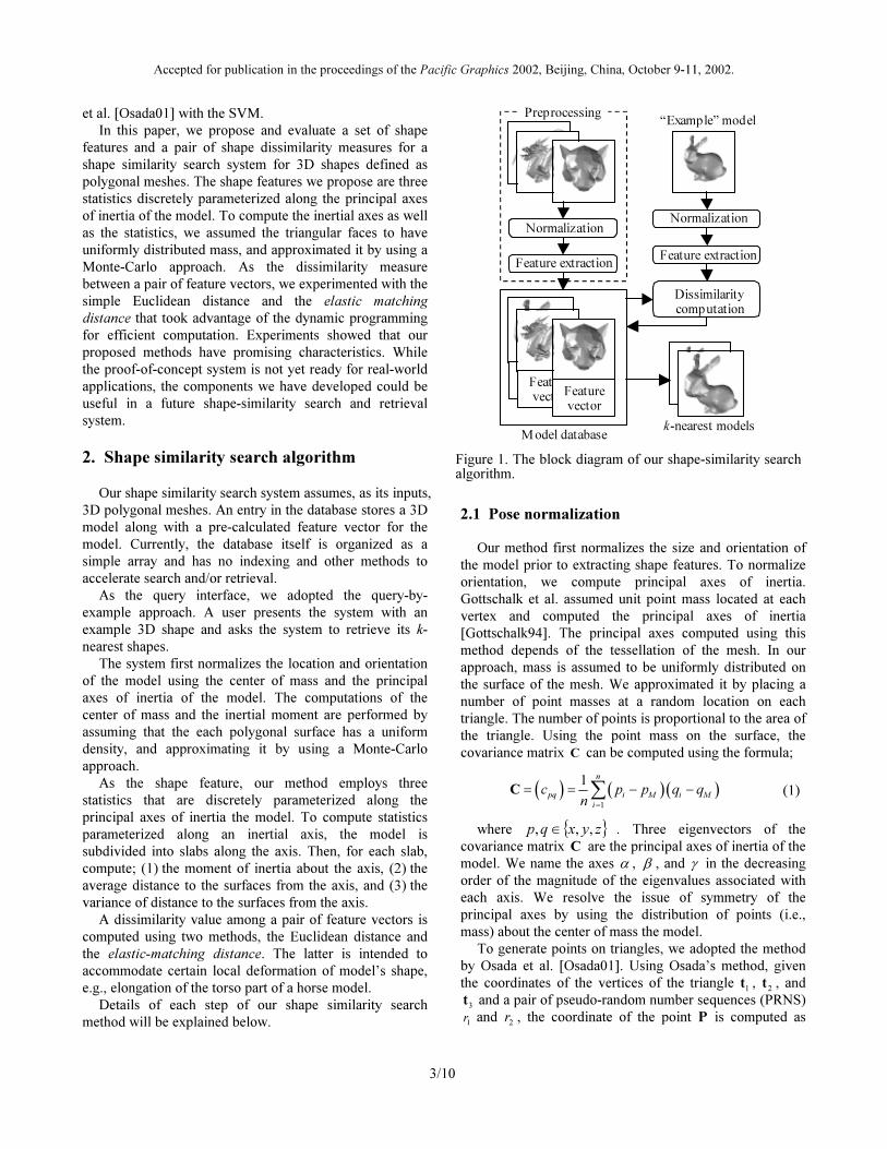
The system first normalizes the location and orientation

of the model using the center of mass and the principal

axes of inertia of the model. The computations of the

center of mass and the inertial moment are performed by

assuming that the each polygonal surface has a uniform

density, and approximating it by using a Monte-Carlo

approach.

As the shape feature, our method employs three

statistics that are discretely parameterized along the

principal axes of inertia the model. To compute statistics

parameterized along an inertial axis, the model is

subdivided into slabs along the axis. Then, for each slab,

compute; (1) the moment of inertia about the axis, (2) the

average distance to the surfaces from the axis, and (3) the

variance of distance to the surfaces from the axis.

A dissimilarity value among a pair of feature vectors is

computed using two methods, the Euclidean distance and

the elastic-matching distance. The latter is intended to

accommodate certain local deformation of model’s shape,

e.g., elongation of the torso part of a horse model.

Details of each step of our shape similarity search

method will be explained below.

2.1 Pose normalization

Our method first normalizes the size and orientation of

the model prior to extracting shape features. To normalize

orientation, we compute principal axes of inertia.

Gottschalk et al. assumed unit point mass located at each

vertex and computed the principal axes of inertia

[Gottschalk94]. The principal axes computed using this

method depends of the tessellation of the mesh. In our

approach, mass is assumed to be uniformly distributed on

the surface of the mesh. We approximated it by placing a

number of point masses at a random location on each

triangle. The number of points is proportional to the area of

the triangle. Using the point mass on the surface, the

covariance matrix C can be computed using the formula;

( ) ( )( )1

1n

pq i M i M

i

c p p q qn

=

= = − −∑C (1)

where { }zyxqp ,,, ∈ . Three eigenvectors of the

covariance matrix C are the principal axes of inertia of the

model. We name the axes α , β , and γ in the decreasing

order of the magnitude of the eigenvalues associated with

each axis. We resolve the issue of symmetry of the

principal axes by using the distribution of points (i.e.,

mass) about the center of mass the model.

To generate points on triangles, we adopted the method

by Osada et al. [Osada01]. Using Osada’s method, given

the coordinates of the vertices of the triangle 1t ,

2t , and

3t and a pair of pseudo-random number sequences (PRNS)

1r and

2r , the coordinate of the point P is computed as

�

Feature vector�Feature

vector�

Nolmalization �

Feature extraction�

�

Preprocessing�

Dissimilarity computation�

“Example” model�

M odel database�

Normalization�

Feature extraction �

k-nearest models�

Feature vector�

Normalization�

Figure 1. The block diagram of our shape-similarity search algorithm.


4/10

follows.

( ) ( ) ( )1 1 1 2 2 1 2 31 1r r r r r= − + − + ⋅P t t t . (2)

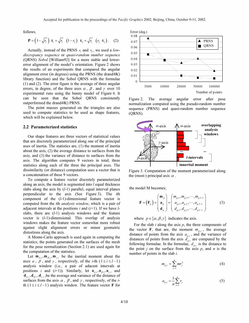
Actually, instead of the PRNS 1r and

2r , we used a low-

discrepancy sequence or quasi-random number sequence

(QRNS) Sobol [William92] for a more stable and lower-

error alignment of the model’s orientation. Figure 2 shows

the results of an experiments that compared the angular

alignment error (in degrees) using the PRNS (the drand48()

library function) and the Sobol QRNS with the formulae

(1) and (2). The error figure is the average of three angular

errors, in degree, of the three axes α , β , and γ over 10

experimental runs using the bunny model of Figure 4. It

can be seen that the Sobol QRNS consistently

outperformed the drand48() PRNS.

The point masses generated on the triangles are also

used to compute statistics to be used as shape features,

which will be explained below.

2.2 Parameterized statistics

Our shape features are three vectors of statistical values

that are discretely parameterized along one of the principal

axes of inertia. The statistics are, (1) the moment of inertia

about the axis, (2) the average distance to surfaces from the

axis, and (3) the variance of distance to surfaces from the

axis. The algorithm computes 9 vectors in total; three

statistics along each of the three the principal axes. The

dissimilarity (or distance) computation uses a vector that is

a concatenation of these 9 vectors.

To compute a feature vector discretely parameterized

along an axis, the model is segmented into l equal thickness

slabs along the axis by (l-1) parallel, equal interval planes

perpendicular to the axis (See Figure 3). The ith

component of the (l-1)-dimensional feature vector is

computed from the ith analysis window, which is a pair of

adjacent intervals at the positions i and (i+1). If we have l-

slabs, there are (l-1) analysis windows and the feature

vector is (l-1)-dimensional. This overlap of analysis

windows makes the feature vector somewhat more robust

against slight alignment errors or minor geometric

distortions along the axis.

A Monte-Carlo approach is used again in computing the

statistics; the points generated on the surfaces of the mesh

for the pose normalization (Section 2.1) are used again for

the computation of the statistics.

Let , , ,

, ,i i iα β γm m m be the inertial moment about the

axes α , β , and γ , respectively, of the i-th (1 1i l≤ ≤ − )

analysis window (i.e., a pair of adacent intervals at

positions i and (i+1)). Similarly, let , , ,

, ,i i iα β γa a a and

, , ,

, ,i i iα β γd d d ,be the average and variance of the distance of

surfaces from the axis α , β , and γ , respectively, of the i-

th (1 1i l≤ ≤ − ) analysis window. The feature vector F for

the model M becomes;

( ),1 ,2 , 1

,1 ,2 , 1

,1 ,2 , 1

, , ,

, , ,

, , ,

p p p p l

p p p p p l

p p p p l

m m m

a a a

d d d

−

−

−

= = =

m

F F a

d

�

�

�

(3)

where { }, ,p α β γ∈ indicates the axis.

For the slab i along the axis p, the three components of

the vector F, that are, the moment ip

m,

, the average

distance of points from the axis ,p i

a , and the variance of

distances of points from the axis ,p i

d are computed by the

following formulae. In the formulae, ,p i

d is the distance to

the point j on the surface from the axis p, and n is the

number of points in the slab i.

2

,

1

n

p i j

j

m mr

=

=∑ (4)

,

1

1n

p i j

j

a r

n=

= ∑ (5)

0

0.01

0.02

0.03

0.04

0.05

0.06

0.07

0.08

5000 10000 20000 50000 100000

Error (deg.)

Number of points

PRNS

QRNS

Figure 2. The average angular error after pose

normalization computed using the pseudo-random number

sequence (PRNS) and quasi-random number sequence

(QRNS).

�

�

�

-axis�α�

-axis�β�

-axis�α�

-axis�γ�

...�

�

�

...�

�

�

l-intervals�

�

innertial moment�

overlapping

analysis

windows�

Figure 3. Computation of the moment parameterized along

the (most-) principal axis α .


5/10

( )2

, ,

1

1

1

n

p i j p i

j

d r an

=

= −

−

∑ (6)

We then normalize the magnitude of the feature vector F

so that 1p p p= = =m a d . This process is repeated for

each of the three axes α , β , and γ .

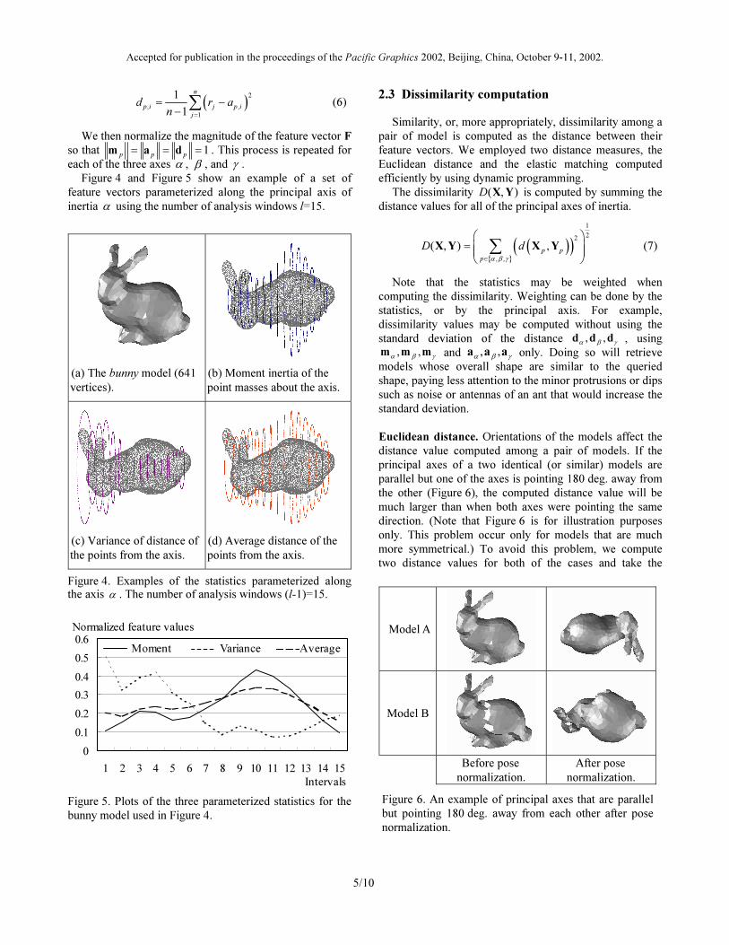
Figure 4 and Figure 5 show an example of a set of

feature vectors parameterized along the principal axis of

inertia α using the number of analysis windows l=15.

(a) The bunny model (641

vertices).

(b) Moment inertia of the

point masses about the axis.

(c) Variance of distance of

the points from the axis.

(d) Average distance of the

points from the axis.

Figure 4. Examples of the statistics parameterized along the axis α . The number of analysis windows (l-1)=15.

0

0.1

0.2

0.3

0.4

0.5

0.6

1 2 3 4 5 6 7 8 9 10 11 12 13 14 15

Intervals

Normalized feature values

Moment Variance Average

Figure 5. Plots of the three parameterized statistics for the

bunny model used in Figure 4.

2.3 Dissimilarity computation

Similarity, or, more appropriately, dissimilarity among a

pair of model is computed as the distance between their

feature vectors. We employed two distance measures, the

Euclidean distance and the elastic matching computed

efficiently by using dynamic programming.

The dissimilarity ( , )D X Y is computed by summing the

distance values for all of the principal axes of inertia.

( )( ){ }

1

22

, ,

( , ) ,p p

p

D d

α β γ∈

= ∑X Y X Y (7)

Note that the statistics may be weighted when

computing the dissimilarity. Weighting can be done by the

statistics, or by the principal axis. For example,

dissimilarity values may be computed without using the

standard deviation of the distance , ,α β γd d d , using , ,α β γm m m and γβα aaa ,, only. Doing so will retrieve

models whose overall shape are similar to the queried

shape, paying less attention to the minor protrusions or dips

such as noise or antennas of an ant that would increase the

standard deviation.

Euclidean distance. Orientations of the models affect the

distance value computed among a pair of models. If the

principal axes of a two identical (or similar) models are

parallel but one of the axes is pointing 180 deg. away from

the other (Figure 6), the computed distance value will be

much larger than when both axes were pointing the same

direction. (Note that Figure 6 is for illustration purposes

only. This problem occur only for models that are much

more symmetrical.) To avoid this problem, we compute

two distance values for both of the cases and take the

Model A

Model B

Before pose

normalization.

After pose

normalization.

Figure 6. An example of principal axes that are parallel

but pointing 180 deg. away from each other after pose

normalization.


6/10

minimum of the two.

The Euclidean distance ( , )euc p p

d X Y between two

feature vectors X and Y are defined as below.

( )( )

( )

11

2 2

, ,

1

11

2 2

, ,

1

1

1, min

1

1

l

p i p i

i

euc p pl

p i p l i

i

ld

l

−

=

−

−

=

−

− = − −

∑

∑

X Y

X Y

X Y

, (8)

where { }, ,p α β γ∈ are the axes of parameterization and l

is the number of intervals.

Elastic-matching distance. Euclidean distance is very

“rigid” and could result in a larger-then-wanted distance

value in some cases. For example, if the torso of an animal

model is somewhat longer than the other animal model

with identical head and tail parts, simple Euclidean

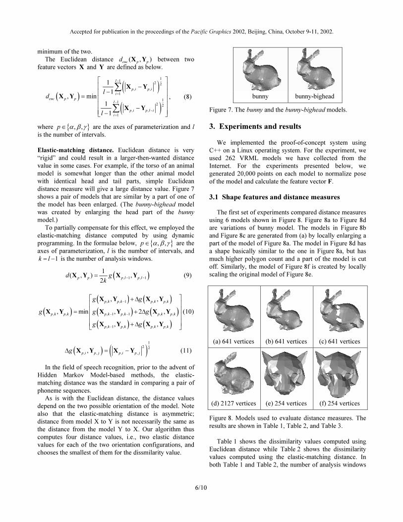
distance measure will give a large distance value. Figure 7

shows a pair of models that are similar by a part of one of

the model has been enlarged. (The bunny-bighead model

was created by enlarging the head part of the bunny

model.)

To partially compensate for this effect, we employed the

elastic-matching distance computed by using dynamic

programming. In the formulae below, { }, ,p α β γ∈ are the

axes of parameterization, l is the number of intervals, and

1k l= − is the number of analysis windows.

( ), 1 , 1

1( , ) ,

2p p p l p ld g

k− −

=X Y X Y (9)

( )

( ) ( )

( ) ( )

( ) ( )

, , 1 , ,

, , , 1 , 1 , ,

, 1 , , ,

, ,

, min , 2 ,

, ,

p k p k p k p k

p k p k p k p k p k p k

p k p k p k p k

g g

g g g

g g

−

− −

−

+∆ = + ∆ +∆

X Y X Y

X Y X Y X Y

X Y X Y

(10)

( ) ( )1

2 2

, , , ,,

p i p j p i p jg∆ = −X Y X Y (11)

In the field of speech recognition, prior to the advent of

Hidden Markov Model-based methods, the elastic-

matching distance was the standard in comparing a pair of

phoneme sequences.

As is with the Euclidean distance, the distance values

depend on the two possible orientation of the model. Note

also that the elastic-matching distance is asymmetric;

distance from model X to Y is not necessarily the same as

the distance from the model Y to X. Our algorithm thus

computes four distance values, i.e., two elastic distance

values for each of the two orientation configurations, and

chooses the smallest of them for the dissmilarity value.

bunny bunny-bighead

Figure 7. The bunny and the bunny-bighead models.

3. Experiments and results

We implemented the proof-of-concept system using

C++ on a Linux operating system. For the experiment, we

used 262 VRML models we have collected from the

Internet. For the experiments presented below, we

generated 20,000 points on each model to normalize pose

of the model and calculate the feature vector F.

3.1 Shape features and distance measures

The first set of experiments compared distance measures

using 6 models shown in Figure 8. Figure 8a to Figure 8d

are variations of bunny model. The models in Figure 8b

and Figure 8c are generated from (a) by locally enlarging a

part of the model of Figure 8a. The model in Figure 8d has

a shape basically similar to the one in Figure 8a, but has

much higher polygon count and a part of the model is cut

off. Similarly, the model of Figure 8f is created by locally

scaling the original model of Figure 8e.

(a) 641 vertices (b) 641 vertices (c) 641 vertices

(d) 2127 vertices (e) 254 vertices (f) 254 vertices

Figure 8. Models used to evaluate distance measures. The

results are shown in Table 1, Table 2, and Table 3.

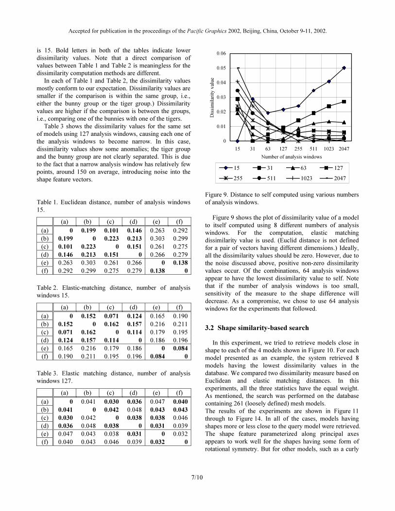
Table 1 shows the dissimilarity values computed using

Euclidean distance while Table 2 shows the dissimilarity

values computed using the elastic-matching distance. In

both Table 1 and Table 2, the number of analysis windows


7/10

is 15. Bold letters in both of the tables indicate lower

dissimilarity values. Note that a direct comparison of

values between Table 1 and Table 2 is meaningless for the

dissimilarity computation methods are different.

In each of Table 1 and Table 2, the dissimilarity values

mostly conform to our expectation. Dissimilarity values are

smaller if the comparison is within the same group, i.e.,

either the bunny group or the tiger group.) Dissimilarity

values are higher if the comparison is between the groups,

i.e., comparing one of the bunnies with one of the tigers.

Table 3 shows the dissimilarity values for the same set

of models using 127 analysis windows, causing each one of

the analysis windows to become narrow. In this case,

dissimilarity values show some anomalies; the tiger group

and the bunny group are not clearly separated. This is due

to the fact that a narrow analysis window has relatively few

points, around 150 on average, introducing noise into the

shape feature vectors.

Table 1. Euclidean distance, number of analysis windows

15.

(a) (b) (c) (d) (e) (f)

(a) 0 0.199 0.101 0.146 0.263 0.292

(b) 0.199 0 0.223 0.213 0.303 0.299

(c) 0.101 0.223 0 0.151 0.261 0.275

(d) 0.146 0.213 0.151 0 0.266 0.279

(e) 0.263 0.303 0.261 0.266 0 0.138

(f) 0.292 0.299 0.275 0.279 0.138 0

Table 2. Elastic-matching distance, number of analysis

windows 15.

(a) (b) (c) (d) (e) (f)

(a) 0 0.152 0.071 0.124 0.165 0.190

(b) 0.152 0 0.162 0.157 0.216 0.211

(c) 0.071 0.162 0 0.114 0.179 0.195

(d) 0.124 0.157 0.114 0 0.186 0.196

(e) 0.165 0.216 0.179 0.186 0 0.084

(f) 0.190 0.211 0.195 0.196 0.084 0

Table 3. Elastic matching distance, number of analysis

windows 127.

(a) (b) (c) (d) (e) (f)

(a) 0 0.041 0.030 0.036 0.047 0.040

(b) 0.041 0 0.042 0.048 0.043 0.043

(c) 0.030 0.042 0 0.038 0.038 0.046

(d) 0.036 0.048 0.038 0 0.031 0.039

(e) 0.047 0.043 0.038 0.031 0 0.032

(f) 0.040 0.043 0.046 0.039 0.032 0

0

0.01

0.02

0.03

0.04

0.05

0.06

15 31 63 127 255 511 1023 2047

Number of analysis windows

Dis

sim

ilar

ity

val

ue

15 31 63 127

255 511 1023 2047

Figure 9. Distance to self computed using various numbers

of analysis windows.

Figure 9 shows the plot of dissimilarity value of a model

to itself computed using 8 different numbers of analysis

windows. For the computation, elastic matching

dissimilarity value is used. (Euclid distance is not defined

for a pair of vectors having different dimensions.) Ideally,

all the dissimilarity values should be zero. However, due to

the noise discussed above, positive non-zero dissimilarity

values occur. Of the combinations, 64 analysis windows

appear to have the lowest dissimilarity value to self. Note

that if the number of analysis windows is too small,

sensitivity of the measure to the shape difference will

decrease. As a compromise, we chose to use 64 analysis

windows for the experiments that followed.

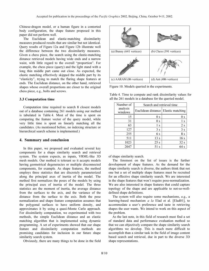
3.2 Shape similarity-based search

In this experiment, we tried to retrieve models close in

shape to each of the 4 models shown in Figure 10. For each

model presented as an example, the system retrieved 8

models having the lowest dissimilarity values in the

database. We compared two dissimilarity measure based on

Euclidean and elastic matching distances. In this

experiments, all the three statistics have the equal weight.

As mentioned, the search was performed on the database

containing 261 (loosely defined) mesh models.

The results of the experiments are shown in Figure 11

through to Figure 14. In all of the cases, models having

shapes more or less close to the query model were retrieved.

The shape feature parameterized along principal axes

appears to work well for the shapes having some form of

rotational symmetry. But for other models, such as a curly


8/10

Chinese-dragon model, or a human figure in a contorted

body configuration, the shape feature proposed in this

paper did not perform well.

The Euclidean and elastic-matching dissimilarity

measures produced results that are similar but not identical.

Query results of Figure 12a and Figure 12b illustrate well

the difference between the two dissimilarity measures.

Given a chess piece, the search using the elastic-matching

distance retrieved models having wide ends and a narrow

waist, with little regard to the overall “proportion”. For

example, the chess piece (query) and the light stand with a

long thin middle part came out close. As expected, the

elastic matching effectively skipped the middle part by its

“elasticity”, trying to match the flaring shape features at

ends. The Euclidean distance, on the other hand, retrieved

shapes whose overall proportions are closer to the original

chess piece, e.g., bolts and screws.

3.3 Computation time

Computation time required to search 8 closest models

out of a database containing 261 models using our method

is tabulated in Table 4. Most of the time is spent on

computing the feature vector of the query model, while

very little time is spent on linearly matching all the

candidates. (As mentioned before, no indexing structure or

hierarchical search scheme is implemented.)

4. Summary and conclusion

In this paper, we proposed and evaluated several key

components for a shape similarity search and retrieval

system. The system expects, as inputs, VRML-like 3D

mesh models. Our method is tolerant so it accepts models

having geometrical degeneracies or multiple disconnected

components, for example. As shape features, the method

employs three statistics that are discretely parameterized

along the principal axes of inertia of the model. The

method first normalizes the poses of the models by using

the principal axes of inertia of the model. The three

statistics are the moment of inertia, the average distance

from the surfaces to the axis, and the variance of the

distance from the surface to the axis. Both the pose

normalization and shape feature computation assumes that

the polygonal surfaces to have uniform density, and

approximates it by using a quasi-Monte Carlo approach.

For dissimilarity computation, we experimented with two

methods, the simple Euclidean distance and an elastic

matching algorithm that is implemented using dynamic

programming. A set of experiments showed that our shape

feature and dissimilarity computation methods are

promising candidates for inclusion in our future shape

similarity search system.

Obviously, there are many things to be done in the field

of shape similarity search.

The foremost on the list of issues is the further

development of shape features. As the demand for the

shape similarity search is diverse, the authors think that not

one but a set of multiple shape features must be recruited

for an effective shape similarity search. We are interested

in the shape features that won’t require pose-normalization.

We are also interested in shape features that could capture

topology of the shape and are applicable to not-so-well-

defined shape definitions.

The system will also require some mechanisms, e.g., a

learning-based mechanism a la Elad et al. [Elad01], to

accommodate a user’s preference and taste in retrieving

shapes the user wants. We intend to work on this aspect of

the problem.

As the last note, in this field of research must find a set

of standard data and performance evaluation method so

that we can objectively compare the shape similarity search

algorithms we develop. This is much more difficult to

accomplish than a similar task in the field of image content

based search and retrieval, due in part to the diverse 3D

shape representations.

(a) Bunny (641 vertices) (b) Chess (391 vertices)

(c) AARAM (86 vertices) (d) Ant (486 vertices)

Figure 10. Models queried in the experiments.

Table 4. Time to compute and rank dissimilarity values for

all the 261 models in a database for the queried model.

Search and retrieval time Number of analysis windows Euclidean distance Elastic matching

15 0 s 0 s

31 0 s 1 s

63 1 s 2 s

127 3 s 3 s

255 6 s 8 s

511 13 s 16 s

1023 25 s 32 s

2047 51 s 64 s


9/10

Acknowledgements

This research has been funded in part by the grant

No. 12680432 from the Ministry of Education, Culture,

Sports, Sciences, and Technology of Japan, and by the

grant from the Okawa Foundation for Information and

Telecommunications. We thank Prof. Shigeo Takahashi for

discussion and providing us with the software collection

gmtools on which our prototype system is based.

References

[Burges98] C. Burges, A Tutorial on Support Vector Machines for Pattern Recognision, Data Mining and Knowledge Discovery, 2, pp. 1-47, 1998.

[Corney02] J. Corney, H. Rea, D. Clark, John Pritchard, M. Breaks, R. MacLeod, Coarse Filter for Shape Matching, IEEE CG&A, pp. 65-73, May/June, 2002.

[Elad00] M. Elad, A. Tal, S. Ar. Directed Search in A 3D Objects Database Using SVM, HP Laboratories Israel Technical Report, HPL-2000-20 (R.1), August, 2000.

[Gottschalk96] Gottschalk, S., Lin, M.C., Manocha, D., OBBTree: A Hierarchical Structure for Rapid Interference Detection, Proc. SIGGRAPH ’96, pp. 171-180, 1996.

[Hilaga01] M. Hilaga, Y. Shinagawa, T. Kohmura, and T. Kunii. Topology Matching for Fully Automatic Similarity Estimation of 3D Shapes. Proc. SIGGRAPH 2001, pp. 203-212, Los Angeles, USA. 2001.

[Ibato02] Masatoshi Ibato, Tomo Otagiri, Ryutarou Ohbuchi, Shape-similarity Search of Three-Dimensional Models Based on Subjective Measures, IPSJ SIG report on Graphics&CAD, Vol. 2002, No. 16 (2002-CG-106), pp. 25-30, February, 2002.

[Igarashi99] Takeo Igarashi, Hidehiko Tanaka, Satoshi Matusoka, Teddy: A Sketching Interface for 3D Freeform Design, Proc. SIGGRAPH ’99, pp. 409-416, 1999.

[Keim99] D. Keim, Efficient Geometry-based Similarity Search of 3D Spatial Databases, Proc. ACM SIGMOD Int. Conf. On Management of Data, pp. 419-430, Philadelphia, PA., 1999.

[McWherter01] D. McWherter, M. Peabody, W. Regli, A. Shokoufandeh, Transformation Invariant Shape Similarity Comparison of Solid Models, Proc. ASME DETC ‘2001, September 2002, Pittsburgh, Pennsylvania.

[Mukai02] S. Mukai, S. Furukawa, M. Kuroda, An Algorithm for Deciding Similarities of 3-D Objects, Proc. ACM Symposium on Solid Modeling and Applications 2002, Saarbrücken, Germany, June 2002.

[Novotni01] M. Novotni, R. Klein. A Geometric Approach to 3D Object Comparison. Proc. Int’l Conf. on Shape Modeling and Applications 2001, pp. 167-175, Genova, Italy, May, 2001.

[Osada01] Osada, T. Funkhouser, B. Chazelle, D. Dobkin. Matching 3D Models with Shape Distributions. Proc. Int’l Conf. on Shape Modeling and Applications 2001, pp. 154-166, Genova, Italy, May, 2001.

[Paquet97] E. Paquet and M. Rioux, Nefertiti: a Query by Content Software for Three-Dimensional Databases Management, Proc. Int’l Conf. on Recent Advances in 3-D Digital Imaging and Modeling, pp. 345-352, Ottawa, Canada, May 12-15, 1997.

[Paquet00] E. Paquet, A. Murching, T. Naveen, A. Tabatabai, M. Roux. Description of shape information for 2-D and 3-D objects. Signal Processing: Image Communication, 16:103-122, 2000.

[Regli00] W. Regli, V. Cicirello, Managing Digital Libraries for Computer-Aided Design, Computer Aided Design, pp. 110-132, Vol. 32, No. 2, 2000.

[Suzuki98] M. T. Suzuki, T. Kato, H. Tsukune. 3D Object Retrieval based on subject measures, Proc. 9th Int’l Conf. and Workshop on Database and Expert Systems Applications (DEXA98), pp. 850-856, IEEE-PR08353, Vienna, Austria, Aug. 1998.

[Suzuki00] M. T. Suzuki, T. Kato, N. Otsu. A similarity retrieval of 3D polygonal models using rotation invariant shape descriptors. IEEE Int. Conf. on Systems, Man, and Cybernetics (SMC2000), Nashville, Tennessee, pp. 2946-2952, 2000.

[Vapnik98] V. N. Vapnik. Statistical Learning Theory. Wiley, 1998.

[Vapnik99] V. N. Vapnik. The Nature of Statistical Learning Theory, Second Edition. Springer, 1999.

[Veltkamp01] R. C. Veltkamp. Shape Matching: Similarity Measures and Algorithms, invited talk, Proc. Int’l Conf. on Shape Modeling and Applications 2001, pp. 188-197, Genova, Italy, May, 2001.

[Vranić01] D. V. Vranić, D. Saupe, and J. Richter. Tools for 3D-object retrieval: Karhunen-Loeve Transform and spherical harmonics. Proc. of the IEEE 2001 Workshop on Multimedia Signal Processing, Cannes, France, pp. 293-298, October 2001.

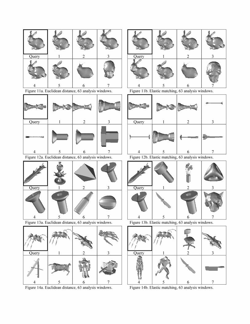
Query 1 2 3 Query 1 2 3

4 5 6 7 4 5 6 7

Figure 11a. Euclidean distance, 63 analysis windows. Figure 11b. Elastic matching, 63 analysis windows.


4 5 6 7 4 5 6 7



4 5 6 7 4 5 6 7



4 5 6 7 4 5 6 7


shape-similarity search of three-dimensional models using

Documents