shared communications channels 6.02 spring 2011 lecture #12

6.02 Spring 2011 Lecture 12, Slide #1

6.02 Spring 2011

Lecture #12

•  shared medium → media access protocol •  time division multiple access (TDMA) •  contention protocols, Alohanet


Shared Communications Channels

•  Basic constraint: avoid collisions between transmitters – Collisions can be detected from corrupted packets

• Wanted: a communications protocol (“rules of engagement”) that ensures good performance overall

Shared channel, e.g., wireless or cable

channel interface

packet queues


“Good” Performance

•  High utilization –  Channel capacity is a limited resource → use it efficiently –  Ideal: use 100% of channel capacity in transmitting packets

–  Waste: idle periods, collisions, protocol overhead

•  Fairness –  Divide capacity equally among requesters

–  But not every node is requesting all the time…

•  Bounded wait –  An upper bound on the wait before successful transmission

–  Important for isochronous communications (e.g., voice/video)

•  Scalability –  Accommodate changing number of nodes, hopefully without

changing implementation of any given node


Sharing Protocols

•  Protocols ≡ “rules of engagement” for good performance –  Known as media access control (MAC) or multiple access control

•  Time division –  Share time “slots” between requesters

–  Prearranged: time division multiple access (TDMA)

–  Not prearranged: contention protocols (e.g., Alohanet). These are interesting because each node operates independently

•  Frequency division –  Give each transmitter its own frequency, receivers choose

“station”

–  Our topic for after spring break

•  Code division –  Uses unique orthogonal pseudorandom code for each transmitter

–  Channel adds transmissions to create combined signal –  Receiver listens to one “dimension” of combined signal using dot

product of code with combined signal.


Utilization

•  Utilization measures the throughput of a channel:

•  Example: 10 Mbps channel, four nodes get throughputs of 1, 2, 2 and 3 Mbps. So utilization is (1+2+2+3)/10 = 0.8.

•  0 ! U ! 1. Utilization can be less than 1 if –  The nodes have packets to transmit (nodes with packets in their

transmit queues are termed backlogged), but the protocol is inefficient.

–  There is insufficient offered load, i.e., there aren’t enough packets to transmit to use the full capacity of the channel.

•  With backlogged nodes, perfect utilization is easy: just let one node transmit all the time! But that wouldn’t be fair…

Uchannel =total throughput over all nodesmaximum data rate of channel


Fairness

•  Many plausible definitions. A standard recipe: –  Measure throughput of nodes = xi, over a given time interval –  Say that a distribution with lower standard deviation is “fairer”

than a distribution with higher standard deviation.

–  Given number of nodes, N, fairness F is defined as

•  1/N ! F ! 1, where F=1/N implies single node gets all the throughput and F=1 implies perfect fairness.

•  We’ll see that there is often a tradeoff between fairness and utilization, i.e., fairness mechanisms often impose some overhead, reducing utilization.

F =xii=1

N!( )

2

N x2ii=1

N!


Abstraction for Shared Medium

•  Time is divided into slots of equal length

•  Each node can start transmission of a packet only at the beginning of a time slot

•  All packets are of the same size and hence take the same amount of time to transmit, equal to some integral multiple of time slots.

•  If the transmissions of two or more nodes overlap, they are said to collide and none of the packets are received correctly. Note that even if the collision involves only part of the packet, the entire packet is assumed to be lost.

•  Transmitting nodes can detect collisions, which usually means they’ll retransmit that packet at some later time.

•  Each node has a queue of packets awaiting transmission. A node with a non-empty queue is said to be backlogged.


Time Division Multiple Access (TDMA)

•  Suppose that there is a centralized resource allocator and a way to ensure time synchronization between the nodes – for example, a cellular base station.

•  For N nodes, give each node a unique index in the range [0,N-1]. Assume each slot is numbered starting at 0.

•  Node i gets to transmit in time slot t if, and only if, t mod N = i. So a particular node transmits once every N time slots.

•  No packet collisions! But unused time slots are “wasted”, lowering utilization. Poor when nodes send data in bursts or have different offered loads.


TDMA for GSM Phones

http://en.wikipedia.org/wiki/Time_division_multiple_access

First slot is used in cell phones to contact tower for slot assignment. Tower can determine appropriate timing advance for each user (accounts for varying distance from tower) so that transmissions won’t overlap at the tower.


Contention Procotols: Alohanet

To improve performance when there are burst data patterns or skewed loads, use a contention protocol where allocation is not predetermined.

Alohanet was a satellite-based data network connecting computers on the Hawaiian islands. One frequency was used to send data to the satellite, which rebroadcast it on a different frequency to be received by all stations. Stations could only “hear” the satellite, so had to decide independently when it was their turn to transmit.


Collision

Success, Idleness, Collisions

•  Throughput = Uncollided packets per time interval •  Utilization = Throughput / Channel Rate = 12/20 = .6

Channel idle time slot


Slotted Aloha

•  Aloha protocol followed by each of N nodes: if a node is backlogged, it sends a packet in the next time slot with probability p.

•  Assume (for now) each packet takes exactly one time slot to transmit (slotted Aloha)

•  Utilization when all nodes backlogged? The probability that exactly one node sends a packet. –  prob(send a packet) = p

–  prob(don’t send a packet) = 1-p

–  prob(only one sender) = p(1-p)N-1

–  There are (N choose 1) = N ways to choose the one sender

Uslotted Aloha = Np(1! p)N!1


Maximizing Utilization

To determine maximum: set dU/dp = 0, solve for p. Result: p = 1/N, so

Umax = (1!1N)N!1

ln (1! 1N

)N!1"

#$

%

&'= (N !1)ln(1! 1

N)

= (N !1)(! 1N!

12N 2 !

13N 3 !…)

= !1+ 1N+

16N 2 +

112N 3 +…

= !1 as N()

N!", Umax !1e# 37%As


Simulation of Slotted Aloha (N=10)

Utilization = .38, Fairness = .98

python PS6_2.py –r –n 10 –p .1 –t 1000

Top: success Bottom: failure


Stabilization: Selecting the Right p

•  Setting p = 1/N maximizes utilization, where N is the number of backlogged nodes.

•  With bursty traffic or nodes with unequal offered loads (aka skewed loads), the number of backlogged is constantly varying.

•  Issue: how to dynamically adjust p to achieve maximum utilization? –  Detect collisions by listening, or by missing acknowledgement

–  Each node maintains its own estimate of p

–  If collision detected, too much traffic, so decrease local p

–  If success, maybe more traffic possible, so increase local p

•  “Stabilization” is, in general, the process of ensuring that a system is operating at, or near, a desired operating point. –  Stabilizing Aloha: finding a p that maximizes utilization as

loading changes.


Binary Exponential Back-off

•  Decreasing p on collision –  Estimate of N (# of backlogged nodes) too low, p too high –  To quickly find correct value use multiplicative decrease:

p ← p/2

–  k collisions in a row: p decreased by factor of 2－k

–  Binary: 2, exponential: k, back-off: smaller p → more time between tries

•  Increasing p on success –  While we were waiting to send, other nodes may have emptied

their queues, reducing their offered load. –  If increase is too small, slots may go idle

–  Try multiplicative increase: p ← min(2*p,1)

–  Or maybe just: p ← 1 to ensure no slots go idle


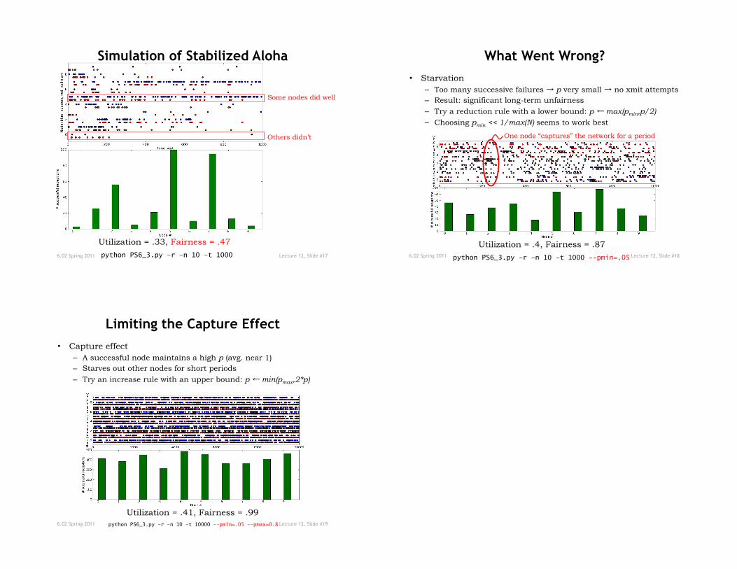
Simulation of Stabilized Aloha

python PS6_3.py –r –n 10 –t 1000


Some nodes did well

Others didn’t


What Went Wrong?

•  Starvation –  Too many successive failures → p very small → no xmit attempts –  Result: significant long-term unfairness

–  Try a reduction rule with a lower bound: p ← max(pmin,p/2)

–  Choosing pmin << 1/max(N) seems to work best

python PS6_3.py –r –n 10 –t 1000 --pmin=.05


One node “captures” the network for a period


Limiting the Capture Effect

•  Capture effect –  A successful node maintains a high p (avg. near 1) –  Starves out other nodes for short periods

–  Try an increase rule with an upper bound: p ← min(pmax,2*p)

python PS6_3.py –r –n 10 –t 10000 --pmin=.05 --pmax=0.8


shared communications channels 6.02 spring 2011 lecture #12

Documents