sharing experiences and learning's of formation...
TRANSCRIPT

Sharing Experiences and Learning's Of Formation Testing
Andrew CarnegieWoodside
Slide 1FEAUS May 2012

Disclaimer and Important Notice
This presentation contains forward looking statements that are subject to risk factors associated with oil and gas businesses. It is believed that the expectations reflected in these statements are reasonable but they may be affectedbusinesses. It is believed that the expectations reflected in these statements are reasonable but they may be affected by a variety of variables and changes in underlying assumptions which could cause actual results or trends to differ materially, including but not limited to: price fluctuations, actual demand, currency fluctuations, drilling and production results, reserve estimates, loss of market, industry competition, environmental risks, physical risks, legislative, fiscal and regulatory developments, economic and financial market conditions in various countries and regions, political risks, project delay or advancement approvals and cost estimatesproject delay or advancement, approvals and cost estimates.
All references to dollars, cents or $ in this presentation are to Australian currency, unless otherwise stated.
References to “Woodside” may be references to Woodside Petroleum Ltd. or its applicable subsidiaries
Slide 2FESAUS 8 May 2012
Acknowledgements
Thanks to Woodside for permission to present
Thanks to FESAUS for the opportunity to present
Thanks for the many folks who have contributed data and technical knowledge that underpin this presentation
Thanks to Russell Ward for several helpful suggestions relating to the presentation
Slide 3FESAUS 8 May 2012
Overview
The focus is on pressure gradients and fluid contacts.
We consider some of the perhaps more unusual issues
• Data QC in an offshore environment
• Quantification of uncertainty in a fluid contacty
• Local examples will be shown that illustrate some of the more unusual effects that can cause uncertainty in interpretation of pressure measurementsthat can cause uncertainty in interpretation of pressure measurements
• Suggestions on optimal pretest volumes will be made
Unless stated otherwise, please assume that any discussion here refers to wells drilled with water based mud.
Slide 4FESAUS 8 May 2012
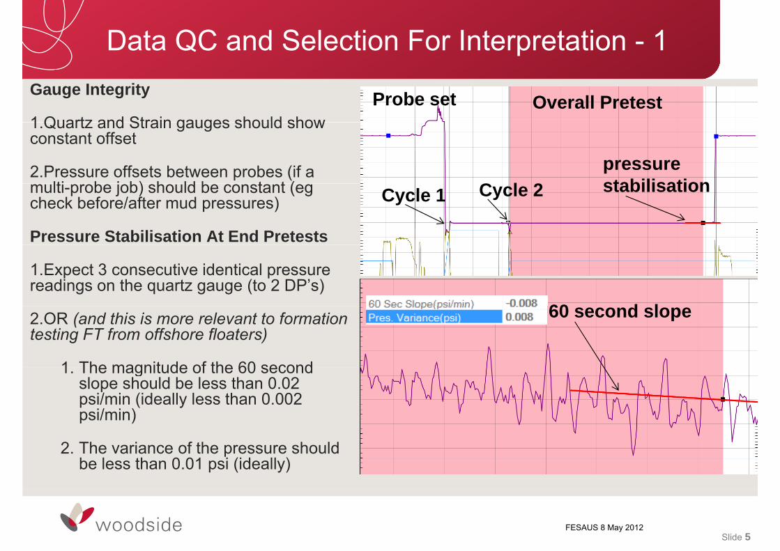
Data QC and Selection For Interpretation - 1Gauge Integrity
1 Quartz and Strain gauges should showOverall PretestProbe set
1.Quartz and Strain gauges should show constant offset
2.Pressure offsets between probes (if a lti b j b) h ld b t t ( C l 2
pressure stabilisationmulti-probe job) should be constant (eg
check before/after mud pressures)
Pressure Stabilisation At End Pretests
Cycle 1 Cycle 2 stabilisation
1.Expect 3 consecutive identical pressure readings on the quartz gauge (to 2 DP’s)
60 d l2.OR (and this is more relevant to formation testing FT from offshore floaters)
1 The magnitude of the 60 second
60 second slope
1. The magnitude of the 60 second slope should be less than 0.02 psi/min (ideally less than 0.002 psi/min)
2. The variance of the pressure should be less than 0.01 psi (ideally)
Slide 5FESAUS 8 May 2012
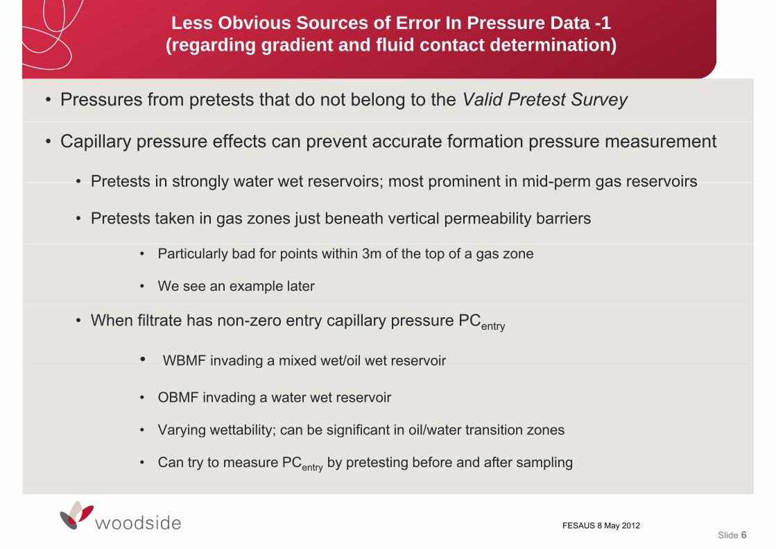
Less Obvious Sources of Error In Pressure Data -1 (regarding gradient and fluid contact determination)
• Pressures from pretests that do not belong to the Valid Pretest Survey
• Capillary pressure effects can prevent accurate formation pressure measurement
• Pretests in strongly water wet reservoirs; most prominent in mid-perm gas reservoirs• Pretests in strongly water wet reservoirs; most prominent in mid-perm gas reservoirs
• Pretests taken in gas zones just beneath vertical permeability barriers
• Particularly bad for points within 3m of the top of a gas zone
• We see an example later
• When filtrate has non-zero entry capillary pressure PCentry
• WBMF invading a mixed wet/oil wet reservoirg
• OBMF invading a water wet reservoir
V i tt bilit b i ifi t i il/ t t iti• Varying wettability; can be significant in oil/water transition zones
• Can try to measure PCentry by pretesting before and after sampling
Slide 6FESAUS 8 May 2012
Less Obvious Sources of Error In Pressure Data -2 (regarding gradient and fluid contact determination)
• Tidal effects in formations that are connected to surface water (ie follow the hydrostatic gradient)gradient)
• Estimated to be up to 1 psi in oil/water legs
• Negligible in gas legs
• Tidal effects complicate multi-well interpretations (eg normalisation of gauges via t t k i if th t i d t b i ilib i )measurements taken in an aquifer that is assumed to be in equilibrium).
• Formation fluid in the FT flowline
• Particularly likely if sampling has occurred, or even large volume pretests in gas zones
Slide 7FESAUS 8 May 2012
Comments On Interpretation Methodology
Regression Model
• Initially assume a straight line model
• Least squares regression where both pressure P and depth Z are variables
• Check biase on error residuals
• Zonal sub-division warranted?
• Curved gradient detected (compositional gradient, other effects)?
• Move to a quadratic or cubic line?
Use a combination of log data, Pressure vs Depth regression and Excess Pressure to delineate gas, oil and water legs
Use a combination of Pressure vs Depth Regression and Excess Pressure To Identify ContactsUse a combination of Pressure vs Depth Regression and Excess Pressure To Identify Contacts
Contacts are either Proven (lie in a sand for which there also exist log saturations) or Unproven
C t U t i t E ti ti th d tComments on Uncertainty Estimation method next
Slide 8FESAUS 8 May 2012

Estimating Uncertainty In Contacts. Several th d d 1methods are used - 1
Statistical Error, SE - use the approach of SPE 99386 – Quantitative Estimate
• SE is an estimate of the allowable uncertainty in the contact, assuming that the
regression errors are unbiased (ie purely statistical)regression errors are unbiased (ie purely statistical).
Uncertainties also assessed by these other means:
• Observations of oil, gas or water at various depths – a qualitative estimate
Log sat rations• Log saturations
• Sampling or Pumping stations
• Determining in the contact depth and associated uncertainty, by constraining the “pressure gradient” with the independently determined expectation of formation fluid density and its associated uncertainty - a qualitative estimate
Slide 9FESAUS 8 May 2012
Estimating Uncertainty In Contacts. Several th d d 2methods are used - 2
A few guidelines on applying the different types of Uncertainty estimates
1) If the contact is Proven, then is possible to choose as follows:
• Uncertainty = MIN(Qualitative Quantitative)Uncertainty MIN(Qualitative , Quantitative)
2) If the contact is Unproven, then it is advisable to carry both Qualitative and Quantitative uncertainty estimatesQuantitative uncertainty estimates
Slide 10FESAUS 8 May 2012

Examples
Objective: To show how tidal corrections are potentially important when interpreting wireline measured pressure data taken in an oil or water zonewireline measured pressure data taken in an oil or water zone
Demonstrate this by a case study on a well X
The formation testing tool discussed here will be called the MDT, for the sake of convenience
But, the example could refer to data from almost any formation testing tool
Slide 11FESAUS 8 May 2012
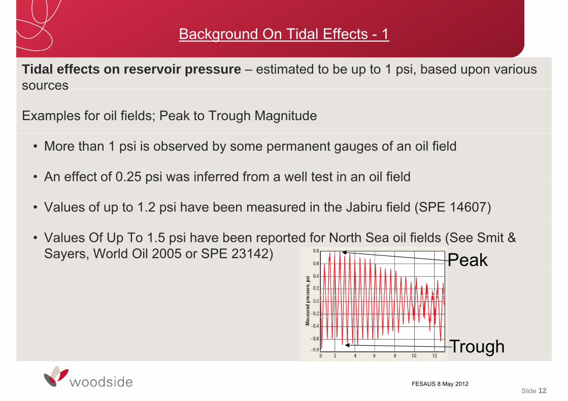
Background On Tidal Effects - 1
Tidal effects on reservoir pressure – estimated to be up to 1 psi, based upon various sourcessources
Examples for oil fields; Peak to Trough Magnitude
• More than 1 psi is observed by some permanent gauges of an oil field
• An effect of 0 25 psi was inferred from a well test in an oil fieldAn effect of 0.25 psi was inferred from a well test in an oil field
• Values of up to 1.2 psi have been measured in the Jabiru field (SPE 14607)
• Values Of Up To 1.5 psi have been reported for North Sea oil fields (See Smit & Sayers, World Oil 2005 or SPE 23142) Peak
Trough
Slide 12FESAUS 8 May 2012
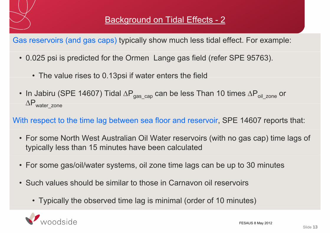
Background on Tidal Effects - 2
Gas reservoirs (and gas caps) typically show much less tidal effect. For example:
• 0.025 psi is predicted for the Ormen Lange gas field (refer SPE 95763).
• The value rises to 0.13psi if water enters the fieldThe value rises to 0.13psi if water enters the field
• In Jabiru (SPE 14607) Tidal Pgas_cap can be less Than 10 times Poil_zone or PPwater_zone
With respect to the time lag between sea floor and reservoir, SPE 14607 reports that:
• For some North West Australian Oil Water reservoirs (with no gas cap) time lags of typically less than 15 minutes have been calculated
• For some gas/oil/water systems, oil zone time lags can be up to 30 minutes
S h l h ld b i il t th i C il i• Such values should be similar to those in Carnavon oil reservoirs
• Typically the observed time lag is minimal (order of 10 minutes)
Slide 13FESAUS 8 May 2012
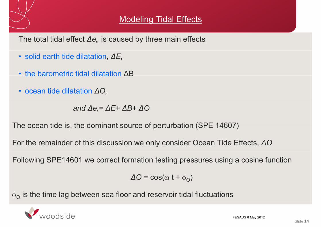
Modeling Tidal Effects
The total tidal effect ∆et, is caused by three main effects
• solid earth tide dilatation, ∆E,
• the barometric tidal dilatation ∆Bthe barometric tidal dilatation ∆B
• ocean tide dilatation ∆O,
and ∆et = ∆E+ ∆B+ ∆O
The ocean tide is the dominant source of perturbation (SPE 14607)The ocean tide is, the dominant source of perturbation (SPE 14607)
For the remainder of this discussion we only consider Ocean Tide Effects, ∆O
Following SPE14601 we correct formation testing pressures using a cosine function
∆O = cos(t + )∆O = cos(t + O)
O is the time lag between sea floor and reservoir tidal fluctuations
Slide 14FESAUS 8 May 2012

Why Correct Pressure Data For Tidal Effects?
Improves formation testing answers
• Reservoir Fluid Density Estimation
• Reduces Free Fluid Contact Uncertainty
• Improves Detection Of Reservoir Compartments
Some other benefitsSome other benefits
• Improved well test and interference test planning
• Assessment of pore volume compressibility by the equation below
Tidal Efficiency R = P i /P fl where both are due to ocean tide effectsTidal Efficiency R Preservoir /Pseafloor, where both are due to ocean tide effects.
Then, it can be shown (eg SPE 103253) that R =)1(3)()1(
CfCppCpp
Cpp and Cf: pore volume and fluid compressibilities respectively
is Poisson’s ratio
)()( fpp
Slide 15FESAUS 8 May 2012

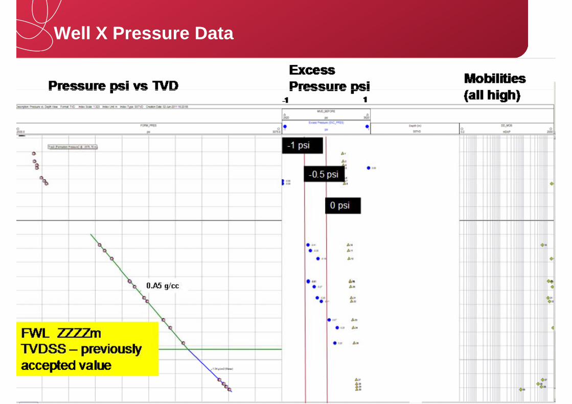
Case Study, Well X Pressure Interpretation
Well X pressure data. A common gradient is proposed between the Upper and Lower sands.
Outstanding issues with the current straight line g ginterpretation
1.Biase in residual errors from upper to lower Sands1.Biase in residual errors from upper to lower Sands
2. Gradient inferred Oil density 0.A5 g/cc. Lab PVT density 0 A65g/cc The difference in density isdensity 0.A65g/cc. The difference in density is significant. Which is correct?
M jMajor consequences:
Upper and Lower Sands may not communicate
Free water level for Lower Sand is has been incorrectly estimated (inaccurate prediction of OOIP)
Slide 16FESAUS 8 May 2012
est ated ( accu ate p ed ct o o OO )
Well X Pressure Data
Slide 17FESAUS 8 May 2012
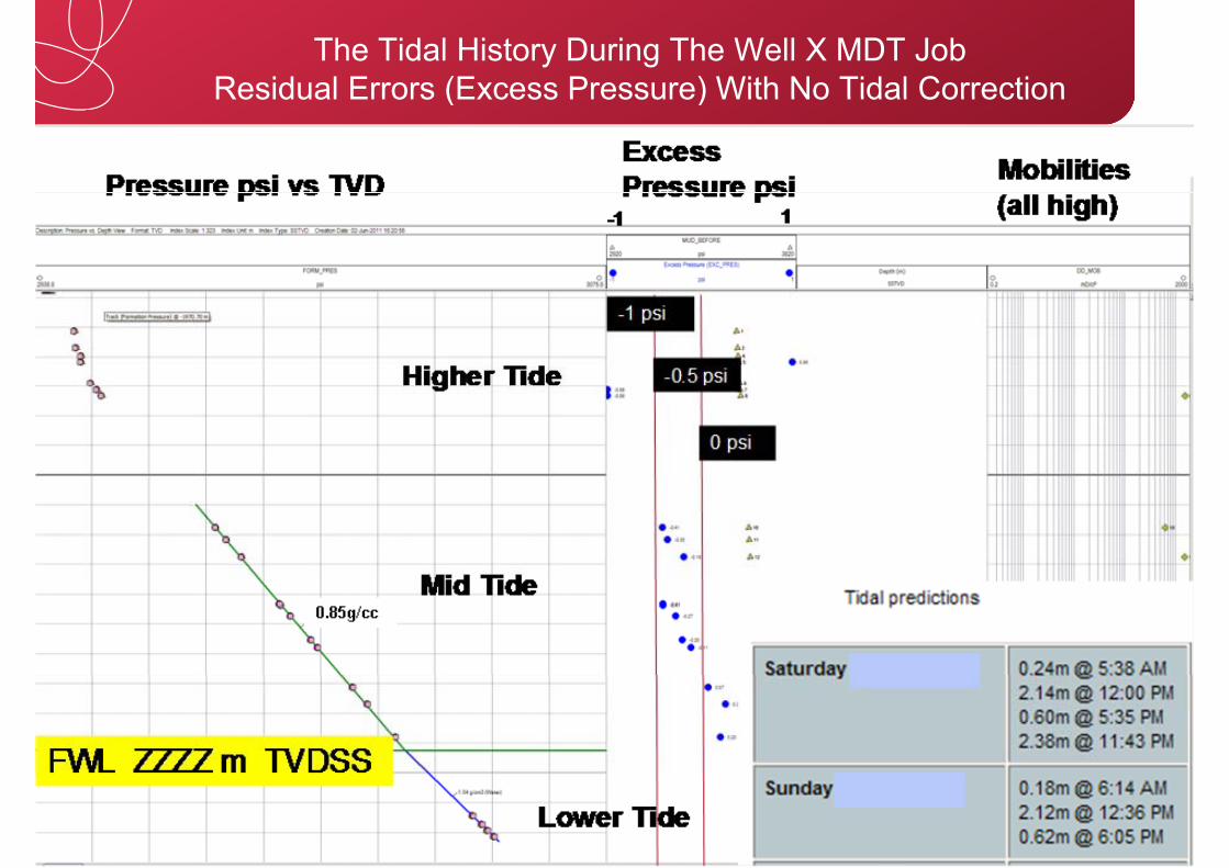
The Tidal History During The Well X MDT JobResidual Errors (Excess Pressure) With No Tidal CorrectionResidual Errors (Excess Pressure) With No Tidal Correction
Slide 18FESAUS 8 May 2012

Apply A Correction Of 0.25 psiPressure Residual Errors Reduce. essu e es dua o s educe
Slide 19FESAUS 8 May 2012
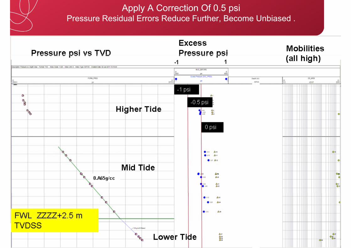
Apply A Correction Of 0.5 psiPressure Residual Errors Reduce Further, Become Unbiased .
Slide 20FESAUS 8 May 2012

FWL and R2 vs Tidal Correction, TC
FWL's and Rsquared (oil zone only) vs tidal correction
A li d Tid l C ti i
-2046 5
-20460 0.1 0.2 0.3 0.4 0.5 0.6 0.7 0.8
0 9999
0.99992Applied Tidal Correction psi
ZZZZ
-2047
-2046.5
0.99988
0.9999
R2
ZZZZ
-2047.5
FWL
0.99986
RZZZZ+1
-2048.5
-2048
0.99982
0.99984
ZZZZ+2
-2049 0.9998
FWL (no TC in w ater zone)
FWL
R2
ZZZZ+3-2049.5
tidal correction amplitude psi
0.99978
ZZZZ+3
Slide 21FESAUS 8 May 2012

Sense Check On Tidal Corrections
The tidal correction applied should give a reasonable value for Cpp (pore volume compressibility).
The properties of the Well X Oil and reservoir arep p
API ~ 20 deg, GOR 330 scf/stb, Tres ~ 58 deg C, Pres ~ 3100 psi.
Above properties suggest fluid compressibility Cf, to be about 3.1e-06 psi-1 (depending upon the correlation used)
Equation for R (Tidal Efficiency) then gives Cpp ~ 4.5e-06 psi-1. This is close to what was expected based upon data from other sources
Cf psi 1 R Poisson R Cpp psi 1Cf psi‐1 R Poisson R Cpp psi‐13.10E‐06 0.38181134 0.32 4.4623E‐06
Slide 22FESAUS 8 May 2012
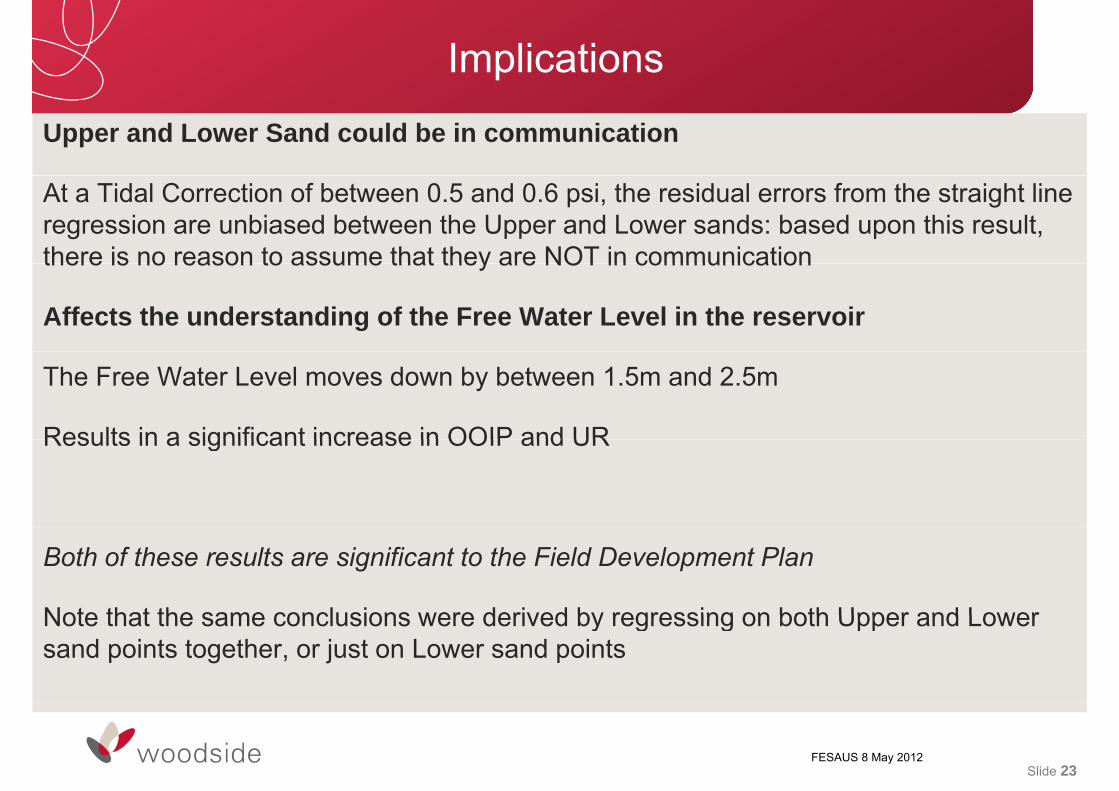
Implications
Upper and Lower Sand could be in communication
At a Tidal Correction of between 0.5 and 0.6 psi, the residual errors from the straight line regression are unbiased between the Upper and Lower sands: based upon this result, there is no reason to assume that they are NOT in communicationthere is no reason to assume that they are NOT in communication
Affects the understanding of the Free Water Level in the reservoir
The Free Water Level moves down by between 1.5m and 2.5m
Results in a significant increase in OOIP and URResults in a significant increase in OOIP and UR
Both of these results are significant to the Field Development Plan
Note that the same conclusions were derived by regressing on both Upper and LowerNote that the same conclusions were derived by regressing on both Upper and Lower sand points together, or just on Lower sand points
Slide 23FESAUS 8 May 2012

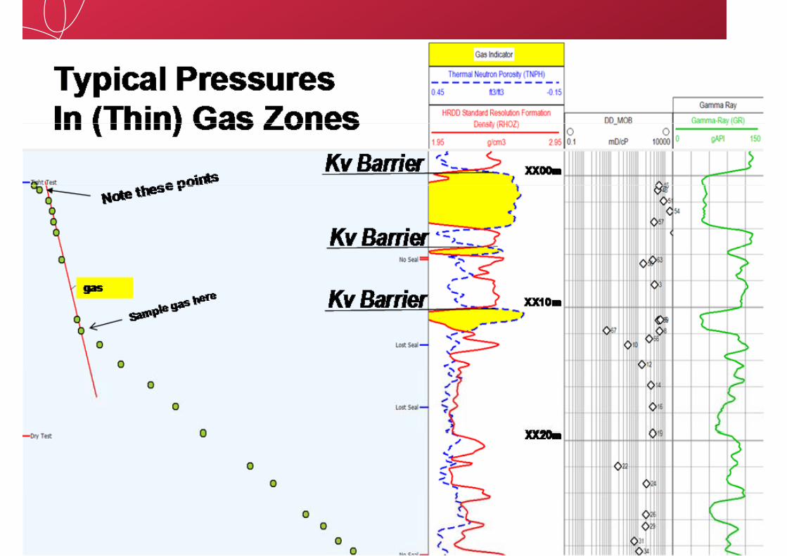
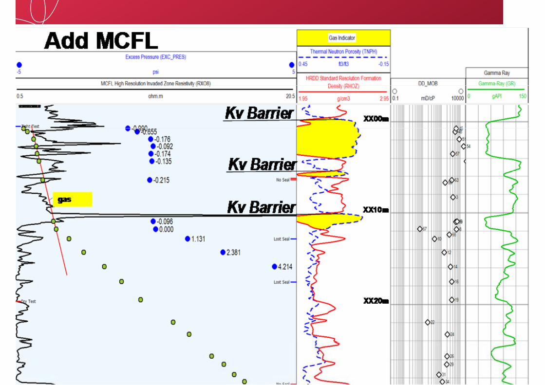
A Common Observation In Thin Gas Zones
Scenario
• Taking pressures in gas zones, beneath, yet close to Kv barriers
• Vertical well drilled with water based mud
• No Supercharging p g g
• High mobility clean sands; Kv/Kx between 0.3 and 1
Slide 24FESAUS 8 May 2012
Slide 25FESAUS 8 May 2012
Slide 26FESAUS 8 May 2012
Slide 27FESAUS 8 May 2012
What does the data suggest? 1
KV barrier exists at XX00m TVD ss
Points close to it have progressively lower excess pressures
• MCFL is the resistivity of the formation close to the formation tester probeMCFL is the resistivity of the formation close to the formation tester probe
• It shows higher resistivity for these points (no deviation effects either; vertical well)
The data implies that filtrate has slumped downwards, away from the Kv barrier, and has been replaced by gas.
• Gas is much lighter than filtrate. Kv in the formation is high. Kv Barrier prevents replenishment of filtrate
There is significant saturation of mobile gas in the invaded zone
A d thi ff t d th d ( t)And this affected the measured pressure (next)
Slide 28FESAUS 8 May 2012
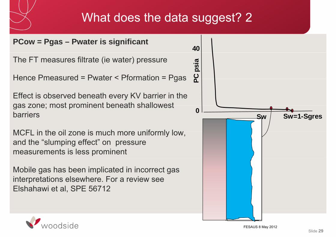
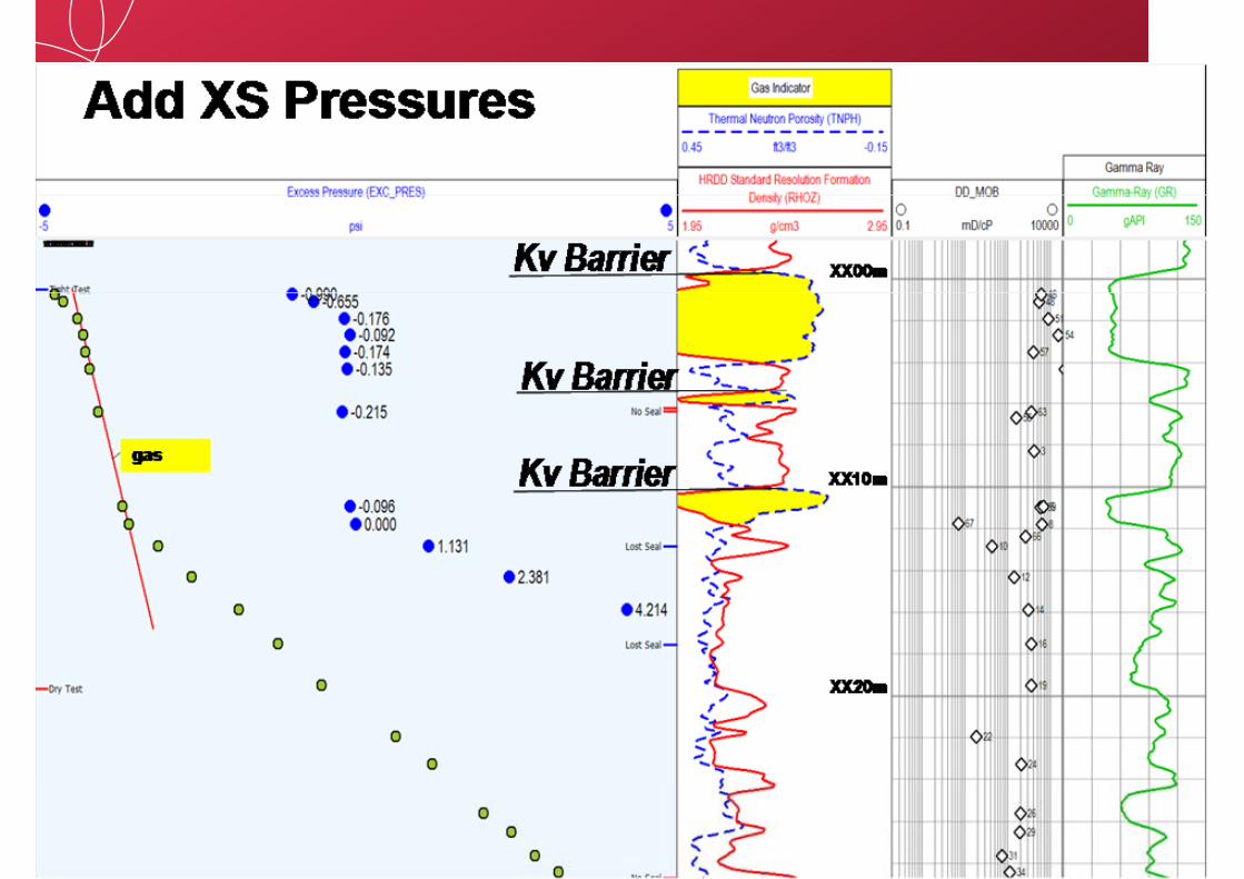
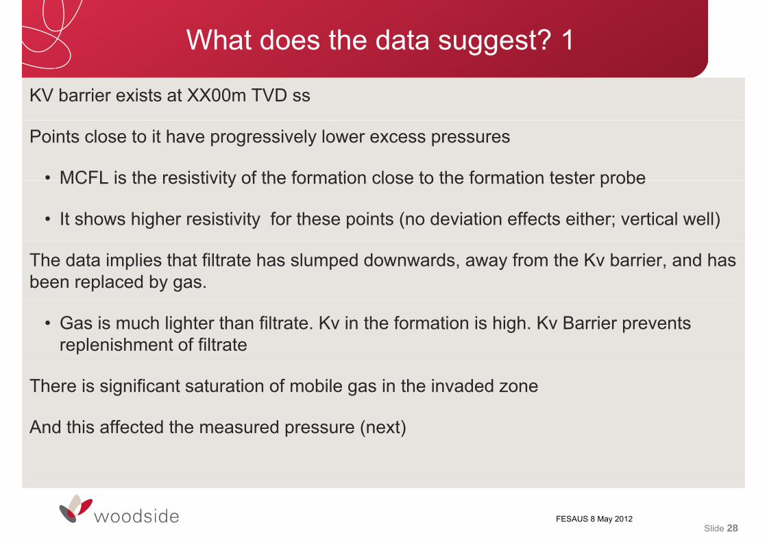
What does the data suggest? 2
PCow = Pgas – Pwater is significant40
The FT measures filtrate (ie water) pressure
Hence Pmeasured = Pwater < Pformation = Pgas PC p
sia
Hence Pmeasured Pwater < Pformation Pgas
Effect is observed beneath every KV barrier in the gas zone; most prominent beneath shallowest
P
gas zone; most prominent beneath shallowest barriers
MCFL in the oil zone is much more uniformly low
Sw Sw=1-Sgres0
MCFL in the oil zone is much more uniformly low, and the “slumping effect” on pressure measurements is less prominent
Mobile gas has been implicated in incorrect gas interpretations elsewhere. For a review see Elshahawi et al, SPE 56712
Slide 29FESAUS 8 May 2012

What does the data suggest? 2
PCow = Pgas – Pwater is significant40
The FT measures filtrate (ie water) pressure
Hence Pmeasured = Pwater < Pformation = Pgas PC p
sia
Hence Pmeasured Pwater < Pformation Pgas
Effect is observed beneath every KV barrier in the gas zone; most prominent beneath shallowest
P
gas zone; most prominent beneath shallowest barriers
MCFL in the oil zone is much more uniformly low
Sw Sw=1-Sgres0
MCFL in the oil zone is much more uniformly low, and the “slumping effect” on pressure measurements is less prominent
Mobile gas has been implicated in incorrect gas interpretations elsewhere. For a review see Elshahawi et al, SPE 56712
Slide 30FESAUS 8 May 2012

What does the data suggest? 2
PCow = Pgas – Pwater is significant40
The FT measures filtrate (ie water) pressure
Hence Pmeasured = Pwater < Pformation = Pgas PC p
sia
Hence Pmeasured Pwater < Pformation Pgas
Effect is observed beneath every KV barrier in the gas zone; most prominent beneath shallowest
P
gas zone; most prominent beneath shallowest barriers
MCFL in the oil zone is much more uniformly low
Sw Sw=1-Sgres0
MCFL in the oil zone is much more uniformly low, and the “slumping effect” on pressure measurements is less prominent
Mobile gas has been implicated in incorrect gas interpretations elsewhere. For a review see Elshahawi et al, SPE 56712
Slide 31FESAUS 8 May 2012
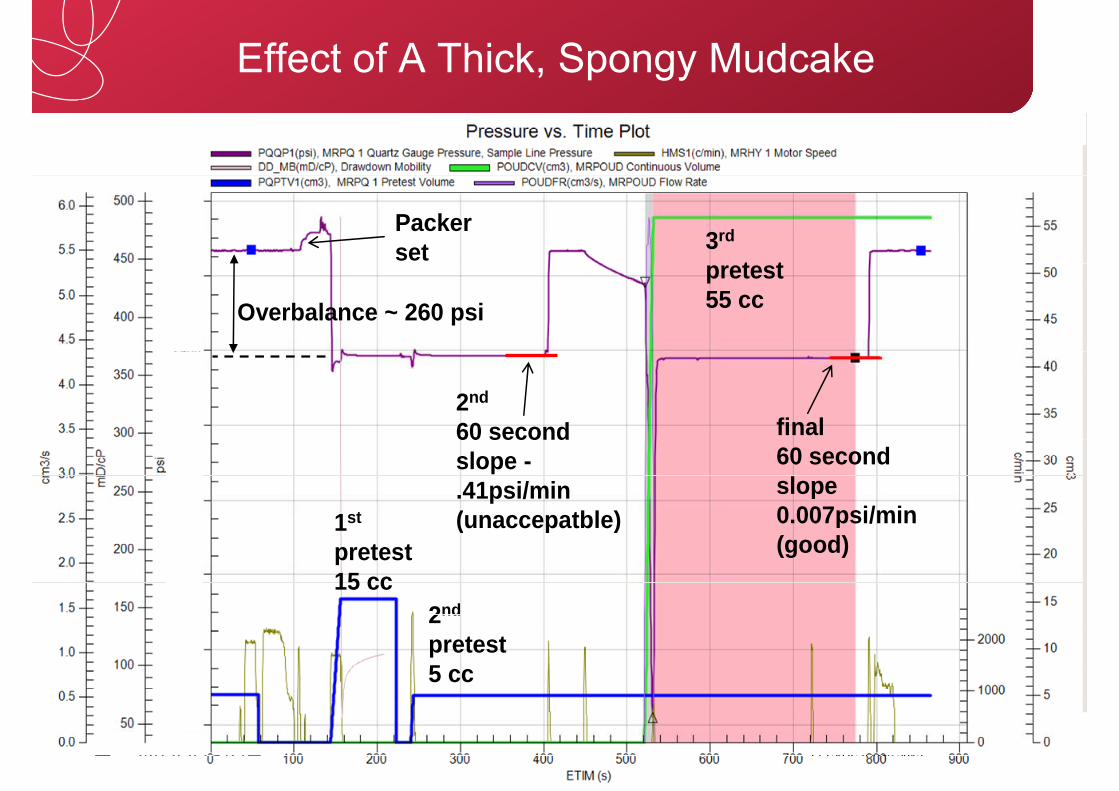
Effect of A Thick, Spongy Mudcake
3rd
t t
Packer set
pretest 55 ccOverbalance ~ 260 psi
final2nd
60 second
1st
60 second slope 0.007psi/min
60 second slope -.41psi/min(unaccepatble)1
pretest 15 cc
2nd
p(good)
(unaccepatble)
2nd
pretest 5 cc
Slide 32FESAUS 8 May 2012
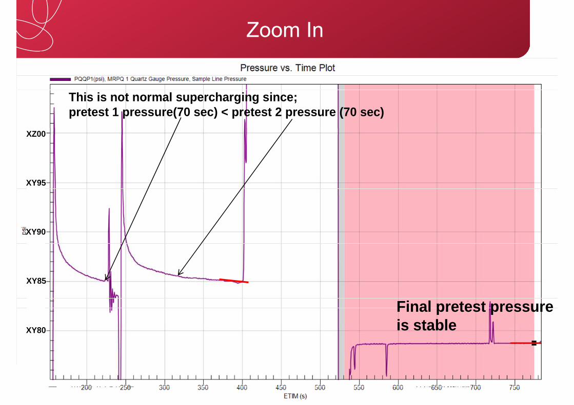
Zoom In
XZ00XZ00
This is not normal supercharging since;pretest 1 pressure(70 sec) < pretest 2 pressure (70 sec)
XZ00
XY95
XZ00
XY95XY95XY95
XY90XY90
XY85XY85
Final pretest pressure XY80XY80 is stable
Slide 33FESAUS 8 May 2012

Conclusions
The mud cake was spongy and contained much filtrate
This was expected because
• The overbalance was low (~ 260 psi).
The mud cake had probably been made thicker becausep y
• The well had been suspended for some days due to a cyclone.
When the probe packer squeezed the mud cake, fluid was expelled into the formation, causing a “build down” over print on the “buildup” from small volume pretests
A large volume pretest (55 cc’s) was sufficient to completely remove this effect
Slide 34FESAUS 8 May 2012
Comments On Optimal Pretest Strategy
How much fluid should be withdrawn from the formation?
And in what sequence?
Easy Answer is “It depends” upon the situation Some basic guidelines below:Easy Answer is It depends upon the situation. Some basic guidelines below:
• Don’t withdraw too much fluid (assume no fluid sampling)
• Only mobile filtrate should be in the volume of investigation of the test and only filtrate should enter the tool.
• Withdraw enough fluid to
1)Break the mud cake)
2)Eliminate mud cake storage effects
3)Understand Dynamic Supercharging DSC: multiple pretests help determine the existence of DSC. They can sometimes even eliminate DSC
Slide 35FESAUS 8 May 2012
The End
Thanks
Slide 36FESAUS 8 May 2012
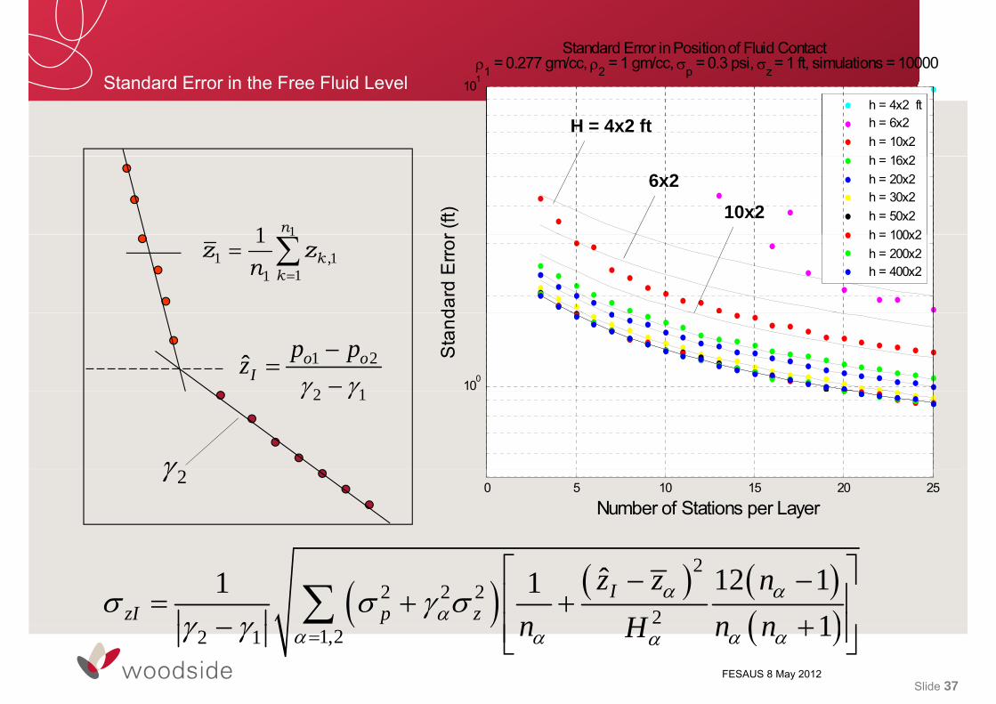
St d d E i th F Fl id L l 1
Standard Error in Position of Fluid Contact 1 = 0.277 gm/cc, 2 = 1 gm/cc, p = 0.3 psi, z = 1 ft, simulations = 10000
Standard Error in the Free Fluid Level 101 h = 4x2 fth = 6x2h = 10x2h 16 2
H = 4x2 ft
r (ft)
h = 16x2h = 20x2h = 30x2h = 50x2h = 100x2
10x2 6x2
11 n
dard
Erro
r h = 100x2h = 200x2h = 400x2
1
1 111
1
,kk
z zn
100
Sta
nd
1 2
2 1
ˆ
o oI
p pz2 1
0 5 10 15 20 25
Number of Stations per Layer
2
22 2 2
2
ˆ 12 11 11
IzI p z
z z nn n nH
Slide 37FESAUS 8 May 2012
1,22 1 1n n nH