sharing longevity risk in life annuity contracts...traditional life annuities • under traditional...

Sharing Longevity Risk in Life Annuity Contracts

© Jorge Miguel Bravo 1

Jorge Miguel Bravo

(University of Évora & Nova University of Lisbon, Portugal) Joint with Pedro Real (UNL) and Carlos Silva (ISEG-UTL)

Annual IFID Centre Conference 2013Toronto, Fields Institute, November 28

Agenda

1. Motivation

2. Options for the payout-phase

3. Managing longevity risk

4. Options embedded in Group Self-Annuitization (GSA) strategies


4. Options embedded in Group Self-Annuitization (GSA) strategies

5. Longevity/Mortality-linked annuities

6. Pricing the embedded options

7. Final remarks & further research

Motivation

• Long-term demographic (ageing) trends will drive to important

changes in the income mix of retirees, due to

§ Reforms in public social security systems

o Increase in contribution rates, reduction in pension/salary ratios or

accrual rates, increase in the retirement age,…


o PAYGO ð NDC Pension systems

§ Market trend away from DB to DC pension schemes

§ Mobility of the workforce, labour market uncertainty,…

§ Increasing pressure on public finances

• The reduction in the retirement income that is “guaranteed” means

that individuals will have to become more self-reliant

Options for the payout-phase

• Main options for the payout phase

1. Self-annuitization (lump-sum payments)

2. Programmed withdrawals

3. Group Self-Annuitization (GSA)


4. Longevity/Mortality linked annuities

5. Traditional life annuities

• The sharing of biometric (longevity/mortality) and market risks

(interest rate, inflation, equity, credit, liquidity,…) between

individuals and annuity providers is different between agreements

Traditional life annuities

• Under traditional whole life annuities the annuitant is entitled to

receive a specified annuity benefit as long as he/she lives,

1. independently of his/her lifetime (individual longevity risk)

2. whatever the lifetimes of the annuitants in the annuity portfolio

or pension fund (aggregate/systematic longevity risk)


3. Whatever the investment yield obtained by the annuity provider

(rate of return guarantee)

• Other options could be added to this product (capital protection)

• Despite their appealing characteristics and economic foundations,

the significance of annuity markets is still limited

Annuity markets constraints: Demand

• The existence of substitutes, namely the «crowding-out» effect induced by “generous” public pensions

• “If I die soon after I retire, the annuity provider will keep my fund”

• Bequest motive, iliquidity

• Annuities are perceived as expensive


• The underestimation of the personal longevity, myopia

• Seen as a financial investment in the accumulation phase

• Insufficient tax incentives

• Lack of understanding of the properties of annuities

• Lack of trust in financial institutions (emerging economies)

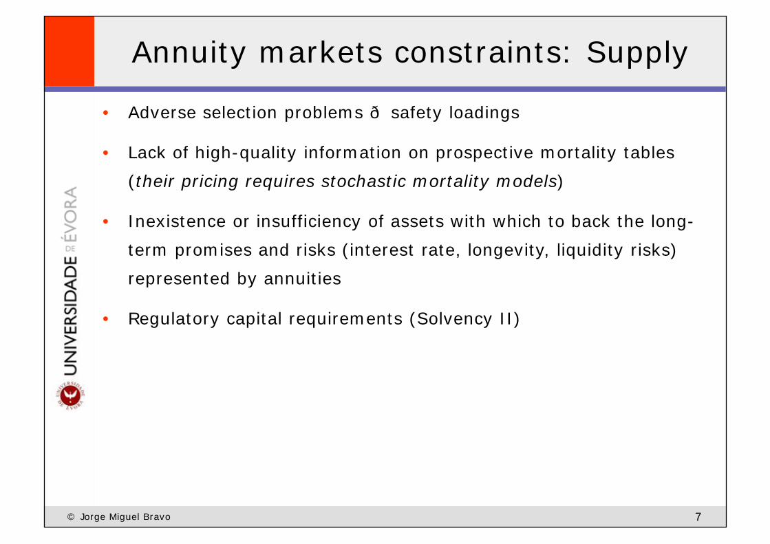
Annuity markets constraints: Supply

• Adverse selection problems ð safety loadings

• Lack of high-quality information on prospective mortality tables (their pricing requires stochastic mortality models)

• Inexistence or insufficiency of assets with which to back the long-term promises and risks (interest rate, longevity, liquidity risks) represented by annuities


represented by annuities

• Regulatory capital requirements (Solvency II)

Managing longevity risk

• Annuity providers (pension funds) have roughly two approaches in

managing longevity risk

1. Transfer the risk to another counterparty

– Insurance-based solutions

– Capital market solutions


– Capital market solutions

– Product design

2. Hedge the risk while retaining it

– Portfolio diversification

– Pricing policy

– Product design

Managing longevity risk

Insurance-basedsolutions

Capital markets-basedsolutions

§ Annuities

§ Buy-in

§ Buy-out

§ Reinsurance

§ Longevity Bonds

§ Extreme mortality structures

(Mortality Bonds)

§ q-Forwards


§ Reinsurance

arrangements

§ q-Forwards

§ Longevity Swaps

§ Longevity Options

§ Life insurance securitization

§ Collateralised longevity

obligations

Product design & Pricing policy

• Conservative pricing policy (higher safety loadings)

• Price differently among individuals according to their specific risk

factors (e.g., smoking) ð contingency loadings

• Reduce the level of investment profit participation

• Annuities with premiums indexed to the evolution of longevity


• Annuities with premiums indexed to the evolution of longevity

• Participating (with-profit GAR) product that shares part of the

emerging profit/loss among surviving policyholders

• Annuities with benefits linked to mortality/longevity

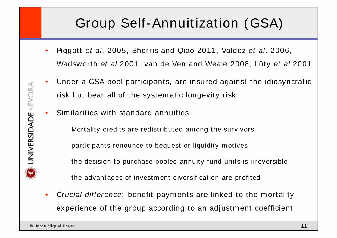
Group Self-Annuitization (GSA)

• Piggott et al. 2005, Sherris and Qiao 2011, Valdez et al. 2006,

Wadsworth et al 2001, van de Ven and Weale 2008, Lüty et al 2001

• Under a GSA pool participants, are insured against the idiosyncratic

risk but bear all of the systematic longevity risk

• Similarities with standard annuities


– Mortality credits are redistributed among the survivors

– participants renounce to bequest or liquidity motives

– the decision to purchase pooled annuity fund units is irreversible

– the advantages of investment diversification are profited

• Crucial difference: benefit payments are linked to the mortality

experience of the group according to an adjustment coefficient

Group Self-Annuitization (GSA)

1. The pool starts at time t=0 with an initial size of lx homogeneous

retirees in the sense of identical age, gender and cohort, identical

monetary amounts and identical risk exposures

2. The annuity arrangement is offered to individuals in exchange for a

single upfront premium

3. The annuity provides an initial level benefit B , paid once a year,


3. The annuity provides an initial level benefit B0, paid once a year,

calculated using an annuity factor accounting for expected mortality

improvements and a flat interest rate

4. At any future moment t, the benefit payment will be determined by

( )

( )0

10

0

1

1

t

F it x i

t tt x

MCA IRA

rpB Bp r

=

+

= × ×+

∏ %

%123 14243

GSA: embedded options

• Assume, without loss of generality, that we disregard the IRA

component in the GSA adjustment formula

• Benefit payments at time t can be expressed as:

1.0

0( ) , if 1= =%%

Ft x

t tt x

pf B Bp


2. ( )

0

0 0

0 0 0

European put option

0 0

0

( ) min( , ) max ;0

max 1 ;0

1 max 1 ;0 , if 1

t t t t

Ft x

t x

F Ft x t x

t x t x

f B B B B B B

pB Bp

p pBp p

= = − −

= − −

= − − <

% % %1442443

%

% %


• Benefit payments at time t can be expressed as (cont’d):

3. ( )

0 0

0 0 0

European call option

0

( ) max( , ) max ;0

1 max 1;0 , if 1

t t t t

F Ft x t x

t x t x

f B B B B B B

p pBp p

= = + −

= + − >

% % %1442443

% %


• Compared with traditional annuities, GSA include embedded options

that may reduce (increase) benefit payments in the future if the

actual survivorship rates are higher (lower) than expected and thus

should cost less (more) an amount equal to the option premium

t x t xp p % %


• The loss on the underlying standard annuity portfolio at time t due

to longevity risk is defined as

• The portfolio loss at time t redistributed among the survivors is

( ) ( )00 0

1( ) [ ( )]

++

=

= − = −∑ %xl

Ft i i x t x t x

iL B I t E I t l B p p


• The portfolio loss at time t redistributed among the survivors is

• The loss “inherited” by each surviving policyholder includes a put

option that depends on ratio of survivorship rates

( )0

000 max 1 ;0

FFt x t x

t x t xx t x t t x

L l B pp p Bl l p

+

+ +

= − = × −

%% % %

GSA: disutility sources

• In a scenario of longevity risk, a pure GSA is expected to pay

decreasing annuity benefits

• The annuitant does not know in advance the rate of return of the

pool, hence it carries some upside/downside risk

• The introduction of uncertainty in annuity benefits will have

implications in consumption/saving behaviour according to the


implications in consumption/saving behaviour according to the

individual’s degree of risk aversion (e.g, CRRA ð precautionary

saving ð annuity with increasing payments)

• The dispersion of future mortality (and investment) rates is ignored

• Annuity providers do not bear any kind of risk

• In a limiting situation there will be no payments for those who

survive beyond the highest attainable age assumed in the life table

Longevity/Mortality-linked annuities

• Questions that need to be addressed

1. who should ultimately bear the longevity risk?

2. At what price?

3. How should we define the benefit adjustment coefficient?


– To the mortality experienced by a specific pool of annuitants, by

the general population or by a mixture of populations?

– To which longevity measure (life expectancy, actuarial value of an

annuity, portfolio reserves and assets)?

– Retrospectively or prospectively?

– With which periodicity?

• Literature

Adjustment based on the number of survivors

• 1. Considering the life table set at time 0, a participation rate

combined with a mandatory conversion into a level life annuity at

some advanced age xmax

[ ]0

1 max1 max 1 ;0 , 0,1 , F

t xt t t t

t x

pB B x xp

α α−

= − × − ∈ <

%


– Annuitants bear all/part longevity risk up to xmax, then the annuity

provider steps up; annuity provider takes the life table risk;

Asymmetric contract, annuitants give up some potential upside

• 2. Considering the life table set at time t

%

1 1 max 1 ;0tF

t xt t t

t x

pB Bp

α−

= − × −

%

Adjustment based on the number of survivors

• 3. Considering the limits set by, e.g., the 9X% confidence interval

for the survival probability

– Only systematic risk is shared

0,

1 1 max 1 ;0UB F

t xt t t

t x

pB Bp

α−

= − −

%


– Only systematic risk is shared

• 4. Or its symmetric version (Cap & Floor) (see also Denuit et al., 2011)

[ ]

[ ]

0 0

0 0

,

1

,

1

1 max 1 ;0 , 0,1 , 1

1 max 1;0 , 0,1 , 1

UB F Ft x t x

t t tt x t x

t LB F Ft x t x

t t tt x t x

p pBp p

Bp pB

p p

α α

η η

−

−

− − ∈ <

= + − ∈ >

% %

% %

Adjustment based on the reference population

• 5. Variants [1] to [4] can be reformulated and be based on the

relation between the expected and observed number of survivors

(or survivorship rates) in the reference population (or a mixture of

populations), e.g.,

[ ]0 0, , , ,

1 max 1 ;0 , 0,1 , 1 UB F POP UB F POPp pB α α

− − ∈ <


In this case, the basis risk (adverse selection effect) is borne by the annuity

provider and less idiosyncratic risk is transferred to individuals

[ ]

[ ]

0 0

0 0

1

, , , ,

1

1 max 1 ;0 , 0,1 , 1

1 max 1;0 , 0,1 , 1

t x t xt t tPOP POP

t x t xt LB F POP UB F POP

t x t xt t t POP

t x t x

p pBp p

Bp pB

p p

α α

η η

−

−

− − ∈ <

= + − ∈ >

% %

% %

Adjustment based on different life tables

• 6. Considering the life table set at time 0 and time t for the

annuitants population

0

1 1 max 1 ;0t

Ft x

t t t Ft x

pB Bp

α−

= − × −


• 7. Or the equivalent design considering population life tables

0 ,

1 ,1 max 1 ;0t

F POPt x

t t t F POPt x

pB Bp

α−

= − × −

Adjustment based on ax ratios

• 8. The benefit is adjusted according to the update in the actuarial

value of a life annuity, as calculated according to an annuity market

life table or a population life table

01

|1 max 1 ;0

|x t

x t

Kt t t

K t

a FB B

a Fα +

+

−

Ε = − × − Ε


Variant: ratio between remaining life expectancies

• 9. Variant, linking annuity market and population life tables

|x tK ta F+

Ε

01

|1 max 1 ;0

|x t

x t

Kt t t POP

K t

a FB B

a Fα +

+

−

Ε = − × − Ε

Adjustment based on asset/reserve ratio

• 10. Adjust, symmetrically, the benefits according to the ratio

between observed assets and portfolio reserves

1 [ ]1 max 1 ;0 tt t P

tt

ABV

BA

α

η

−

− × −

= + −


In this case, all of the biometric and financial risks may be borne by the

annuitants, depending on the participation rate coefficient

• 11. Previous variants considering also financial market risks

1 [ ]1 max 1;0tt t P

t

ABV

η−

+ −

Pricing the embedded options

• A key condition for the development of longevity-linked products

and markets is the development of generally agreed stochastic

mortality models

– Discrete-time (e.g., Lee-Carter model & extensions)

– Continuous-time (SDE for the spot/forward mortality surface)


• How to determine the market price for longevity risk?

– Risk-neutral valuation approach

– Distortion approaches (Wang transform)

– Use classic premium principles (e.g., standard deviation principle)

– Sharpe ratio

– Consumption CAPM, Mean-variance and Risk minimization strategies

Pricing the embedded options

• European call option

• European put option

( ) ( )0max ;0r T t FQt t x t xc E e p p− − = − %

( ) ( )0max ;0r T t FQt t x t xc E e p p− − = − %


• American call option

• American put option

( ) ( )0, ,sup max ;0r t FQ

t t x t xC E e p pττ τ

τ ζ

− −

∈

= − %

( ) ( )0, ,sup max ;0r t FQ

t t x t xP E e p pττ τ

τ ζ

− −

∈

= − %

Stochastic mortality modelling

Model Formula

M1 (Poisson-Lee-Carter) (1) (2) (2),ln( )x t x x tm kβ β= + ⋅

M2 (Renshaw-Haberman Cohort-Lee-Carter)

(1) (2) (2) (3) (3),ln( )x t x x t x t xm kβ β β γ −= + ⋅ + ⋅

M3 (APC, Currie 2006) (1) (2) (3),

1 1ln( )x t x t t xx x

m kn n

β γ −= + ⋅ + ⋅


x xn n

M5 (CBD) (1) (2),log ( )x t t tit q k k x x= + −

M6 (CBD cohort) (1) (2) (3),log ( )x t t t t xit q k k x x γ −= + − +

M7 (CBD quadratic age effect + cohort)

(1) (2) (3) 2 2 (4), ˆlog ( ) (( ) )x t t t t x t xit q k k x x k x x σ γ −= + − + − − +

M8 (CBD decreasing cohort effect)

(1) (2) (3),log ( ) ( )x t t t t x cit q k k x x x xγ −= + − + −

Relational models for mortality

• If the use of internal models for longevity risk is recommended (or

allowed), you may need to resort to Brass-type relational models

for life table construction

• General formulation

( ) ( )( ) ( )ˆ ˆg g REFq f q f xβ ε= + + +


g(.) = log, logit, log(log),…

• Parameters estimated by WOLS or ML

• If you use Monte Carlo Simulation (MCS) methods to price options

you may need a double-bootstrap approach

( ) ( )( ) ( ), 0 1 , 2 ,ˆ ˆg g REFx t x t x tq f q f xβ ε= + + +


• Model the survival probability using affine-jump diffusion processes

• Example: Feller equation

1( , ) ( , ) , , i.i.d

tN

t t t t t t i ii

dX t X dt t X dW dJ Jδ σ ε ε=

= + + = ∑

( ) ( ) ( )d t a t dt dW t dJµ µ σ µ= + +


• dJt is a Poisson process with constant jump-arrival intensity; jump

sizes follow a double asymmetric exponential distribution

( ) ( ) ( )x t x t x t td t a t dt dW t dJµ µ σ µ+ + += + +

1 2

1 1

1 { 0} 2 { 0}1 2

1 2 1 2 1 2

1 1( )

, , , 0, 1

z zf z e I e Iυ υπ πυ υ

π π υ υ π π

−

≥ <

= +

≥ + =


• Assuming that the survival probability can be represented by an

exponential affine function, we can get a closed-formula solution

with

( )( ) exp ( ) ( )· ( )T t x t x tp t A B tτ τ µ− + += +

2 21( ) , 2 , , ,e a aB aκτ κ κ

τ κ σ α α− + −

= = + = =


[

2 20 1

0 1

0 1 0 1 0 1 0 1 1 11

0 1 0 1 1 1

0 2 0 12 0 1

0 2 1 2 0 2

1( ) , 2 , , ,2 2

( )[ln( ) ln( ( )( )( ) ( )( )

( ) ln( )( ) ( )( )

ln

e a aB ae

eA

κτ

κτ

κ κτ κ σ α α

α α

α τ ν α α α α α ν α ντ ηπ

α ν κ α ν α ν

α τ ν α αηπ α α

α ν κ α ν α ν

− + −= = + = =

+

+ + − − + += + − − +

++ + − + + − +

+ }0 2 1 2( ( )eκτα ν α ν ητ+ + − −

Final remarks

• Providers of traditional life annuities are exposed to idiosyncratic

and systematic longevity risks and financial market risks

• Designing longevity/mortality-linked annuities with risk sharing

mechanisms is one of the potential solutions to manage the risk

• When designing the contract, we should take into account the


nature of the risk (idiosyncratic/systematic), the capacity of

annuitants to absorb it and the trade-off between risk and the price

of the embedded options

• Pricing the contract requires sound stochastic mortality models

• Pricing the embedded options requires estimating the market price

of longevity risk and may demand the use of MCSM

Further research

• Determine the “optimal” level of annuitization and risk sharing in

longevity-linked annuities

• Assess the price and the risks of the alternative contract

specifications using Monte Carlo Simulation methods

• Estimate the impact of these contract designs on capital


requirements

• Conduct an enquiry to perceive the receptivity of individuals to

these risk sharing mechanisms

THANK YOU


Jorge Miguel Bravo

University of Évora & Nova University of Lisbon, Portugal

E-mail: [email protected] / [email protected]

Toronto, IFID Centre, Fields Institute, November 28, 2013

mailto:[email protected]

mailto:[email protected]

sharing longevity risk in life annuity contracts...traditional life annuities • under traditional...

Documents