shatthik barua master’s thesis, spring 2017

Inverse covariance matrixestimation for the global minimumvariance portfolio

Shatthik BaruaMaster’s Thesis, Spring 2017

This master’s thesis is submitted under the master’s programme Modellingand Data Analysis, with programme option Finance, Insurance and Risk, atthe Department of Mathematics, University of Oslo. The scope of the thesisis 60 credits.

The front page depicts a section of the root system of the exceptionalLie group E8, projected into the plane. Lie groups were invented by theNorwegian mathematician Sophus Lie (1842–1899) to express symmetries indifferential equations and today they play a central role in various parts ofmathematics.

Abstract

The estimation of inverse covariance matrices plays a major role in portfolio opti-mization, for the global minimum variance portfolio in mean-variance analysis it isthe only parameter used to determine the asset allocation. In this thesis I proposeto of use the graphical lasso methodology to directly estimate the inverse covariancematrix, and apply it to the global minimum variance portfolio. The results indicatethat the graphical lasso provides better out-of-sample portfolio variance than thetraditional sample estimator.

Acknowledgement

First and foremost, I would like to thank my supervisors Ingrid Kristine Glad andNils Lid Hjort for their patience and feedback. I would also like to thank my friendsand family for their support and positive distractions during the thesis work.

1

Contents

1 Introduction 41.1 Outline . . . . . . . . . . . . . . . . . . . . . . . . . . . . . . . . . . . 5

2 Portfolio optimization 62.0.1 Portfolio return . . . . . . . . . . . . . . . . . . . . . . . . . . 62.0.2 Shorting . . . . . . . . . . . . . . . . . . . . . . . . . . . . . . 7

2.1 Markowitz . . . . . . . . . . . . . . . . . . . . . . . . . . . . . . . . . 72.2 Mean-variance portfolio analysis . . . . . . . . . . . . . . . . . . . . . 82.3 Feasible region . . . . . . . . . . . . . . . . . . . . . . . . . . . . . . 9

3 Return distribution 163.1 Data . . . . . . . . . . . . . . . . . . . . . . . . . . . . . . . . . . . . 17

4 Covariance 204.1 The covariance matrix . . . . . . . . . . . . . . . . . . . . . . . . . . 204.2 Estimation error . . . . . . . . . . . . . . . . . . . . . . . . . . . . . 20

4.2.1 Sample covariance matrix . . . . . . . . . . . . . . . . . . . . 224.3 Precision matrix . . . . . . . . . . . . . . . . . . . . . . . . . . . . . . 224.4 Estimation . . . . . . . . . . . . . . . . . . . . . . . . . . . . . . . . . 22

4.4.1 Regression . . . . . . . . . . . . . . . . . . . . . . . . . . . . . 234.4.2 Sparsity . . . . . . . . . . . . . . . . . . . . . . . . . . . . . . 234.4.3 Graphical lasso . . . . . . . . . . . . . . . . . . . . . . . . . . 25

5 Sparsity structure 275.0.1 Graph Generation . . . . . . . . . . . . . . . . . . . . . . . . . 285.0.2 Simulate from structure . . . . . . . . . . . . . . . . . . . . . 30

6 Tuning parameter 336.0.1 Methods . . . . . . . . . . . . . . . . . . . . . . . . . . . . . . 336.0.2 Predicting power vs graph recovery . . . . . . . . . . . . . . . 366.0.3 Best tuning parameter method . . . . . . . . . . . . . . . . . 38

7 Experimental Results 427.0.1 Simulated data . . . . . . . . . . . . . . . . . . . . . . . . . . 427.0.2 Real data . . . . . . . . . . . . . . . . . . . . . . . . . . . . . 46

8 Concluding remarks 518.1 Further research . . . . . . . . . . . . . . . . . . . . . . . . . . . . . . 51

2

Appendix A 55A.1 Portfolio return . . . . . . . . . . . . . . . . . . . . . . . . . . . . . . 55A.2 Estimation . . . . . . . . . . . . . . . . . . . . . . . . . . . . . . . . . 55A.3 Regression . . . . . . . . . . . . . . . . . . . . . . . . . . . . . . . . . 57A.4 Sparsity . . . . . . . . . . . . . . . . . . . . . . . . . . . . . . . . . . 58A.5 Graphical lasso . . . . . . . . . . . . . . . . . . . . . . . . . . . . . . 59

Appendix B R-code 61B.1 Support functions . . . . . . . . . . . . . . . . . . . . . . . . . . . . . 61B.2 Predicting power vs graph recovery . . . . . . . . . . . . . . . . . . . 67B.3 Best tuning parameter method . . . . . . . . . . . . . . . . . . . . . . 70B.4 Simulated data . . . . . . . . . . . . . . . . . . . . . . . . . . . . . . 72B.5 Real data . . . . . . . . . . . . . . . . . . . . . . . . . . . . . . . . . 77

3

Chapter 1

Introduction

The theoretical foundation for how an investor should invest in risky assets was laidby the economist Harry Markowitz in 1952. In Markowitz theory the investor’s port-folio can be seen as function of two parameters, the vector of the expected returnsof the risky assets µ and the covariance matrix of the returns Σ. And for this rea-son, it is often referred to as mean-variance portfolio analysis. The mean-varianceframework, serves as the foundation for many theories which are still relevant to-day, such as the Capital Asset Pricing Model (CAPM). In practice µ and Σ areunknown and has to be estimated from historical data or expectations about thefuture. This means that precision of these estimates is uncertain and estimationerror can be made. Studies show that estimation errors lead to poor out-of-sampleportfolio performance, and that portfolios are highly sensitive to estimates of meansand covariance. To circumnavigate the problem of estimation error one can onlyfocus on the estimation of covariance matrix and ignore the expected returns, sinceit is shown the errors in estimates of the expected returns have a bigger impacton portfolio than of covariance matrix. When you only focuses on the estimationof Σ, the optimal portfolio becomes the global minimum variance portfolio, whichis a portfolio with the smallest possible variance of all portfolios. The global min-imum variance portfolio can be seen as a function of one parameter, Σ, or moreprecisely Σ−1. Several methods have been proposed in the literature to estimate theglobal minimum variance portfolio, but most of the focus on the estimation of Σinstead of estimating Σ−1 directly. Σ−1 also called the precision matrix has a spe-cific mathematical interpretation, the elements in Σ−1 contains information aboutthe partial correlation between variables. One can think of this as a measure ofhow correlated two assets are, given the influence of a set of other assets has beenconsidered, and if the normal distribution is assumed as the distribution of the assetreturns, then a partial correlation of 0 implies conditional independence. Given theidea that conditional independence implies a 0 in Σ−1 it is natural to think of theuse of regularization methods to estimate Σ−1. In this thesis I will explore how thegraphical lasso method can be used to estimate Σ−1 and how well it performs forthe estimation global minimum variance portfolio.

4

1.1 OutlineI will start off by giving an introduction to portfolio optimization and mean-varianceportfolio analysis in chapter 2. Then the data that will be used in this thesis andsome of its statistical properties will be presented in chapter 3. In chapter 4 thetopic of covariance, covariance estimation and inverse covariance estimation willbe discussed and the graphical lasso method will be presented. Chapter 5 will gothrough methods used in the simulations and Chapter 6 will discuss the topic oftuning parameter selection for the graphical lasso. In Chapter 7 analysis and resultswill be presented and concluding remarks will be in chapter 8.The software used throughout this thesis is the statistical programing language R,all scrips used in the analysis will be included in the Appendix.

5

Chapter 2

Portfolio optimization

How to invest financial resources is one of the the classical problems of finance.Investors try to allocate their available resources to the assets that will maximizethe value of the invested funds and at the same time eliminate the risk of losses. Anasset is an investment instrument that can be bought and sold. One concept mostinvestors are aware of is the relationship between risk and return, that there is apositive relationship between the risk and the return of a financial asset. In otherwords, when the risk of an asset increases, so does its return. This means that ifan investor is taking on more risk, he is expected to be compensated with a higherreturn. How to find the optimal trade-off between risk and return is described inthe field of mathematical finance under portfolio theory. Portfolio theory was firstdeveloped by Harry Markowitz[1] in the 1950s and his work formed the foundationof modern finance. Before going further into the portfolio theory I will define someof the basic concepts that will be used throughout this thesis.

2.0.1 Portfolio return• Let I denote the investment, the monetary value the investor wants to invest.

• The possible assets that can be invested in are 1, ..., P assets.

• Let Si(t) denote the price of asset i at time t

• Let Ii be the value invested in asset i, i ∈ 1, ..., P such that I =∑P

i=1 Ii.

• Define wi = IiIto be the proportion invested in asset i,

∑Pi=1wi = 1

At time t = 0 we have the value I at our disposal, we split I and invest Ii fori = 1, ..., P in the different assets, this gives us the amount Mi in asset i such thatIi = Si(0)Mi. The value of our portfolio at time t, P (t), can then be expressed as

P (t) =P∑i=1

Si(t)Mi

we see that at t = 0, the value will be our initial investment I, P (0) = I. A quantitythat is important, is the return, which is the gain or loss of an investment. We definethe one period return of asset i as Ri(t),

6

Ri(t) =Si(t)− Si(t− 1)

Si(t− 1)

and the portfolio return as Rp(t),

Rp(t) =P (t)− P (t− 1)

P (t− 1)

For t = 1 we can express the portfolio return Rp(t) as a weighted average of theasset returns, see Appendix

Rp(1) =P (1)− P (0)

P (0)=

P∑i=1

wiRi(1)

2.0.2 ShortingSometimes it is possible to sell an asset that you do not own by short selling theasset. Short selling (shorting) involves borrowing an asset from a lender and thenselling the borrowed asset to a buyer. Then at a later time, you purchase the assetand return it to the lender. Let us say you borrow Mi amount of asset i at timet = 0, we denote borrowing as −Mi. The asset can be sold for −MiSi(0) = −Ii.Notice that by shorting asset i we open up more capital Ii for investing of otherassets, since we can re-invest the value we get from selling the borrowed asset att = 0 in other assets. At time t when it is time to give back the borrowed assets,you have to buy −Mi of asset i for price Si(t), −MiSi(t) = −Ii(t). The profitmade is −Ii(t) − (−Ii) = −Ii(t) + Ii. We see that we have a positive profit whenSi(0) > Si(t). So by shorting assets can have negative asset allocations −Ii andportfolio weights −wi. Shorting assets can be risky since there is no upper boundon Si(t), which can result in unlimited loss. While when buying an asset the loss isbounded by that the asset price cannot be negative.

2.1 MarkowitzIn 1952 the economist Harry Markowitz laid the foundation for portfolio optimiza-tion in his paper, Portfolio Selection[1]. The theory presented in the paper is oftenreferred to as mean-variance portfolio analysis, it analyzes how wealth can be opti-mally invested in assets which differ in regard to their expected return and risk[2].Markowitz showed that under certain given conditions, the choice of a portfolio canbe reduced to balancing the expected return of the portfolio and its variance[2]. Andthat it is possible to reduce risk through diversification such that the risk of the port-folio, measured as its variance, will depend not only on the individual variances ofthe return on different assets, but also on the pairwise covariances of all assets. Thepractice of taking returns as well as risk into account when making investment deci-sions was well known before Markowitz, but he was the first to develop a rigorouslyformulated mathematical framework for portfolio optimization[2]. Harry Markowitzwas awarded the Nobel Prize in Economic Sciences in 1990 for his work in portfolioselection.

7

2.2 Mean-variance portfolio analysisIn this chapter, I will present the key concepts, assumptions, and quantities ofMarkowitz mean-variance model.

The main quantity of focus in the mean-variance model is the portfolio return overa singe period.

Rp =P∑i=1

wiRi(1)

At time t = 0 we decide how to allocate our wealth between the P risky assets andthen evaluate the return at time t = 1. By a risky asset, I mean assets that havestochastic return R = (R1, ..., RP )T over the period. I will drop the time notationhere, Ri = Ri(1), since we only consider one period.

The proportion of wealth invested in asset is represented by the P dimensionalvector w = (wi, .., wp)

T , here wi is the proportion invested in asset i. It is assumedthat the investor will invest all of the wealth at his disposal ,

∑pi=1 wi = 1, and that

short selling is allowed, wi can be negative. Since asset returns are stochastic theinvestor will not know the returns at time t = 1, but it is assumed that the investorknows the expectation, variance and covariance of the asset return.The expected value of the asset return at the end of the period is given by

E[R] = µ = (µ1, ..., µP )T

and the variance and covariance of the asset returns is

Cov(R) = Σ

Here Σ is the covariance matrix with the asset variance on the diagonal, Σii =V ar(Ri), and the covariance between assets on the off-diagonal Σij = Cov(Ri, Rj).From the knowledge of µ and Σ we can derive the expected return and variance ofthe portfolio. The investor expected portfolio return will be

µp = E[Rp] =P∑i=1

wiRi = wTµ

and the portfolio variance is

(σp)2 = V ar(Rp) = wTΣw

The problem the investor is faced with is how to allocate his wealth in the differentassets (wi), which results in different Rp, µp, (σp)2. Markowtiz [3] shows how to tooptimally select the weights w given the assumptions that the investor will:

• Maximize portfolio return, given a risk level

• Minimize portfolio risk, given a return level

Here the expected portfolio return µp is used to represent the portfolio return andthe portfolio variance (σp)2 is used to represent portfolio risk. From the assumptions

8

of the investor, the investor will only be interested in portfolios that Markowtiz callsefficient. An efficient portfolio is a portfolio having simultaneously the smallestpossible variance for its given level of expected return rate and the largest possibleexpected return for its given level of risk[3].

2.3 Feasible regionAll the portfolios an investor can construct are defined by the possible combinationsof weights w, which we will call the weight space. The weight space of an P-assetportfolio is

WP ={w :

P∑i=1

wi = 1}

By plotting the weight space we can see that for P = 2, WP is a line defined by(α, 1− α) for α ∈ R

Figure 2.1: weight space P = 2

And more generally for P ≥ 3, the space WP is an P − 1 dimensional plane inRP passing through the P standard unit basis vectors[3].

9

Figure 2.2: weight space P = 3

The set of all pairs (√

(σp)2(w), µp(w)) for all possible combinations of w is calledthe feasible region

FP ={

(σp(w), µp(w)) : w ∈ WP

}Here σp(w) denotes the standard deviation of the portfolio given weights w, σp(w) =√

(σp)2(w) =√wTΣw.

For P = 2 the weight space maps into FP the right branch of a hyperbola. Andwhen P ≥ 3, FP≥3 feasible region an unbounded region whose boundary is the rightbranch of a hyperbola. It can be shown that the points on the boundary of thefeasible region correspond to unique portfolio weights w, while it exists infinitelymany portfolio weights for any point inside the feasible region[4].

Figure 2.3: Feasible region P = 2,P = 3

10

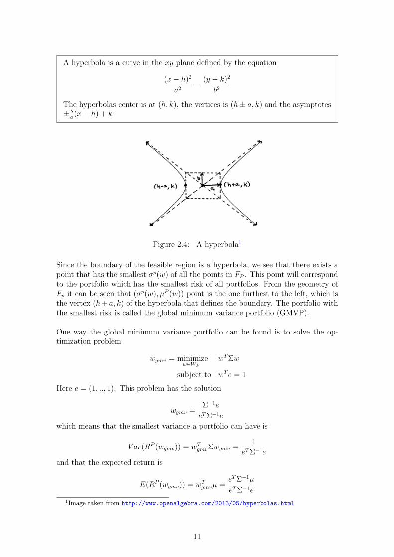
A hyperbola is a curve in the xy plane defined by the equation

(x− h)2

a2− (y − k)2

b2

The hyperbolas center is at (h, k), the vertices is (h± a, k) and the asymptotes± ba(x− h) + k

Figure 2.4: A hyperbola1

Since the boundary of the feasible region is a hyperbola, we see that there exists apoint that has the smallest σp(w) of all the points in FP . This point will correspondto the portfolio which has the smallest risk of all portfolios. From the geometry ofFp it can be seen that (σp(w), µP (w)) point is the one furthest to the left, which isthe vertex (h+ a, k) of the hyperbola that defines the boundary. The portfolio withthe smallest risk is called the global minimum variance portfolio (GMVP).

One way the global minimum variance portfolio can be found is to solve the op-timization problem

wgmv = minimizew∈WP

wTΣw

subject to wT e = 1

Here e = (1, .., 1). This problem has the solution

wgmv =Σ−1e

eTΣ−1e

which means that the smallest variance a portfolio can have is

V ar(RP (wgmv)) = wTgmvΣwgmv =1

eTΣ−1e

and that the expected return is

E(RP (wgmv)) = wTgmvµ =eTΣ−1µ

eTΣ−1e

1Image taken from http://www.openalgebra.com/2013/05/hyperbolas.html

11

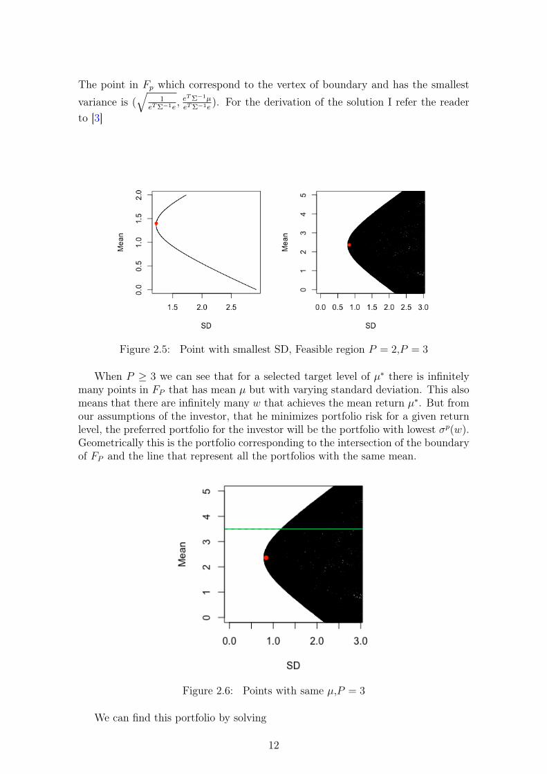
http://www.openalgebra.com/2013/05/hyperbolas.html

The point in Fp which correspond to the vertex of boundary and has the smallest

variance is (√

1eTΣ−1e

, eTΣ−1µeTΣ−1e

). For the derivation of the solution I refer the readerto [3]

Figure 2.5: Point with smallest SD, Feasible region P = 2,P = 3

When P ≥ 3 we can see that for a selected target level of µ∗ there is infinitelymany points in FP that has mean µ but with varying standard deviation. This alsomeans that there are infinitely many w that achieves the mean return µ∗. But fromour assumptions of the investor, that he minimizes portfolio risk for a given returnlevel, the preferred portfolio for the investor will be the portfolio with lowest σp(w).Geometrically this is the portfolio corresponding to the intersection of the boundaryof FP and the line that represent all the portfolios with the same mean.

Figure 2.6: Points with same µ,P = 3

We can find this portfolio by solving

12

w∗ = minimizew∈WP

wTΣw

subject to wTµ = µ∗,

wT e = 1

Which is the solution

w∗ =BΣ−1e− AΣ−1µ∗ + µ∗(CΣ−1µ∗ − AΣ−1e)

D

where

A = µTΣ−1e

B = µTΣ−1µ

C = eTΣ−1e

D = BC − A2

For the derivation of the solution see[3]. The minimum variance of a portfoliowith mean µ∗ will be

(σp(w∗))2 = (w∗)TΣw∗ =µ∗C − 2µ∗A+B

D

From this we can find the the minimum variance for a portfolio with any level ofexpected return µp, and with some algebraic manipulation[3] we can express therelation between the mean and the variance as

(σp)2√1C

2 −(µp − A

C)2√

DC2

2 = 1

which is a hyperbola in the (σp, µp) space, with center at (0, AC

),vertecies (± 1√C, AC

))

and asymptotes ±√

DCpσ+ A

C, and we see that the left vertex of the hyperbola is the

same as the global minimum variance portfolio point, ( 1√C, AC

) = (√

1eTΣ−1e

, eTΣ−1µeTΣ−1e

).

13

Figure 2.7: Boundary of feasible region,P = 3

From the assumptions of the investor, he will only invest in efficient portfolios,which are portfolios having simultaneously the smallest possible variance for its givenlevel of expected return rate and the largest possible expected return for its givenlevel of risk. We showed how to find portfolios having the smallest possible variancefor its given level of expected return, but these portfolios will not necessarily beefficient. To see this we can select the targeted expected return lower then theglobal minimum variance portfolios expected return, µ∗ < eTΣ−1µ

eTΣ−1e.

Figure 2.8: a portfolio on the boundary of the hyperbola is not necessarily efficient

Here it is possible to select portfolios with higher expected return and with thesame standard deviation by moving vertically up in the plane, which means that the

14

portfolio is not efficient. From this we see that if we want an efficient portfolio thetargeted expected return has to be µ∗ ≥ eTΣ−1µ

eTΣ−1e, which means that every boundary

point of FP which is on the upper half of the global minimum variance point willcorrespond to an efficient portfolio. The set off all points that as efficient portfoliosis called the efficient frontier, which can be defined as

EFP ={

(

√µpC − 2µpA+B

D,µp) : µp ≥ A

C

}The weight space of the efficient portfolio is

WEP ={w∗ =

BΣ−1e− AΣ−1µ∗ + µ∗(CΣ−1µ∗ − AΣ−1e)

D: µ∗ ≥ A

C

}

Figure 2.9: The efficient frontier

From the efficient frontier we get the theoretical foundation for the risk-rewardtradeoff, the only way an investor can get higher expected return is take on morerisk.

15

Chapter 3

Return distribution

The main quantities of interest in the mean-variance model is the portfolio returnand its first two moments µp and (σp)2. As Rp is a weighted average of the individualasset returns RP =

∑Pi=1wiRi, the statistical properties of Rp derives form Ri, where

Ri is defined as Ri = Si(1)−Si(0)Si(0)

. This is often called the arithmetic return. Althoughthe arithmetic return is intuitive and easy to understand, there are several drawbacksthat makes arithmetic returns difficult to work with.

1. The future price of the asset Si(1) = Si(0)(1 + Ri(1)) given by the return Ri

can be negative if Ri < −1

2. Return is not symmetric Si(0)(1 +Ri(1))((1−Ri(1))) 6= Si(0)

3. Non additivity of multiple periods∑T

i=1 Ri(t) 6= Ri(T ), Ri(T ) = −1+∏T

i=1(Ri(t)+1). Which means that if we assume that one period returns Ri(1) are i.i.d withthe normal distribution, then the return of longer periods Ri(T ) will not havenormal distribution.

Another return which is often used instead for financial assets is the geometric return

ri = log(Si(1)

Si(0))

which gives the future price as Si(1) = Si(0) exp ri, and where the the relation be-tween the returns are ri = log(1 +Ri).The geometric return corrects all the drawbacks mentioned above, and for this rea-son it is standard in financial analysis to use geometric returns. It is often assumedthat geometric returns have constant expectation and variance, that they are seriallyindependent, and that they are normally distributed[5]. For example in the famousBlack & Scholes model[6], which is used to price options, assumes that the price ofa stock follows a geometric Brownian motion Si(1) = Si(0)eµi+σiB(1), which resultsin normal distributed returns. Here B(t) is a Brownian motion.

Even though geometric returns are easier to work with, and is the standard infinancial analysis, they have one major drawback when it comes to portfolio the-ory. This is that geometric portfolio return cannot be written as weighted sum ofthe geometric asset returns, rp 6=

∑Pi=1wiri[5]. But when the the asset returns are

relatively small, which is the case when the period length is small, the geometric

16

and arithmetic return will be similar[5] log(1 + Ri) ∼ Ri. From this similarity theportfolio return can approximately be written as a wighted sum rp ∼

∑Pi=1wiri[7].

Figure 3.1: Arithmetic returns plotted against geometric returns, when ‖Ri| ≤ 0.10the difference is small

The normality of the returns is often assumed in financial modeling, but it is iswidely known these returns are known to have a distribution that is more peaked andhas fatter tails than the normal distribution[5]. Despite being recognized as overlysimplistic, the assumption of normality has appeal due to that it leads to closedform solutions for many financial problems, it is easy to implement since need onlymake two assumptions for each asset mean and variance and one assumption for thecovariance of each pair. And it somewhat models the return realistically while beingvery simple.

Assumption: We will in this thesis assume that assume that the geometric re-turns follows a multivariate Gaussian distribution, r ∼ N(µ,Σ).

3.1 DataThe assets I will consider in this thesis are stocks from the Norwegian stock exchangetraded on Oslo Børs, at the time of which this thesis is written there are about 190stocks traded on the exchange. The historical data collected on these stocks spansfrom late 2010 to this day(may 2017) where the observations are collected on a dailybasis, the stock prices collected are the end of day closing prices1.

1All prices was extracted from http://www.netfonds.no/, see Appendix for script

17

http://www.netfonds.no/

Figure 3.2: Plot of all stock prices and 5 most traded stocks on Oslo Børs in thelog-scale

If we look at the sample quantiles of the arithmetic returns 98% of the observedreturns lies between −0.09, 0.11, which means that the difference of the arithmeticand geometric returns is small and that we can approximate the arithmetic returnswith geometric.

Table 3.1: Sample quantiles of arithmetic returns0 % 1 % 2 % 3 % 4 % 5 % 6 % 7 % 8 % 9 %-0,8787879 -0,09001943 -0,06839772 -0,05797101 -0,05063291 -0,04545455 -0,04142156 -0,03816794 -0,03517588 -0,0327868910 % 11 % 12 % 13 % 14 % 15 % 16 % 17 % 18 % 19 %-0,03070175 -0,02879581 -0,02702703 -0,02545455 -0,024 -0,02272727 -0,02142857 -0,02024291 -0,01917808 -0,0181818220 % 21 % 22 % 23 % 24 % 25 % 26 % 27 % 28 % 29 %-0,01724138 -0,0163254 -0,01538462 -0,01454545 -0,01376147 -0,01298701 -0,01229942 -0,01156069 -0,01086957 -0,0101863830 % 31 % 32 % 33 % 34 % 35 % 36 % 37 % 38 % 39 %-0,00958206 -0,008955224 -0,008379888 -0,0078125 -0,007220217 -0,006622517 -0,006042296 -0,005454545 -0,004926108 -0,00448430540 % 41 % 42 % 43 % 44 % 45 % 46 % 47 % 48 % 49 %-0,004065041 -0,003613948 -0,003115265 -0,002570694 -0,001917582 -0,000636902 0 0 0 050 % 51 % 52 % 53 % 54 % 55 % 56 % 57 % 58 % 59 %0 0 0 0 0 0 0 0,000928186 0,002118644 0,00271739160 % 61 % 62 % 63 % 64 % 65 % 66 % 67 % 68 % 69 %0,003271538 0,003763441 0,004222658 0,004651163 0,005128205 0,005759585 0,006369427 0,007003379 0,007653061 0,00823421870 % 71 % 72 % 73 % 74 % 75 % 76 % 77 % 78 % 79 %0,008849558 0,00952381 0,01016518 0,01086957 0,01162791 0,01242236 0,01315789 0,01396648 0,01480836 0,0157232780 % 81 % 82 % 83 % 84 % 85 % 86 % 87 % 88 % 89 %0,01671309 0,01769912 0,01873935 0,01980198 0,02097902 0,02230483 0,0237069 0,02527076 0,02702703 0,0288713990 % 91 % 92 % 93 % 94 % 95 % 96 % 97 % 98 % 99 %0,03097345 0,03333333 0,03609023 0,03936903 0,04322767 0,04794521 0,05436573 0,06309148 0,07734807 0,1065574100 %4

We also see that the distribution of the geometric returns agrees with existingfindings, that the geometric return distribution for the assets are more peaked andhas fatter tails than the normal distribution.

18

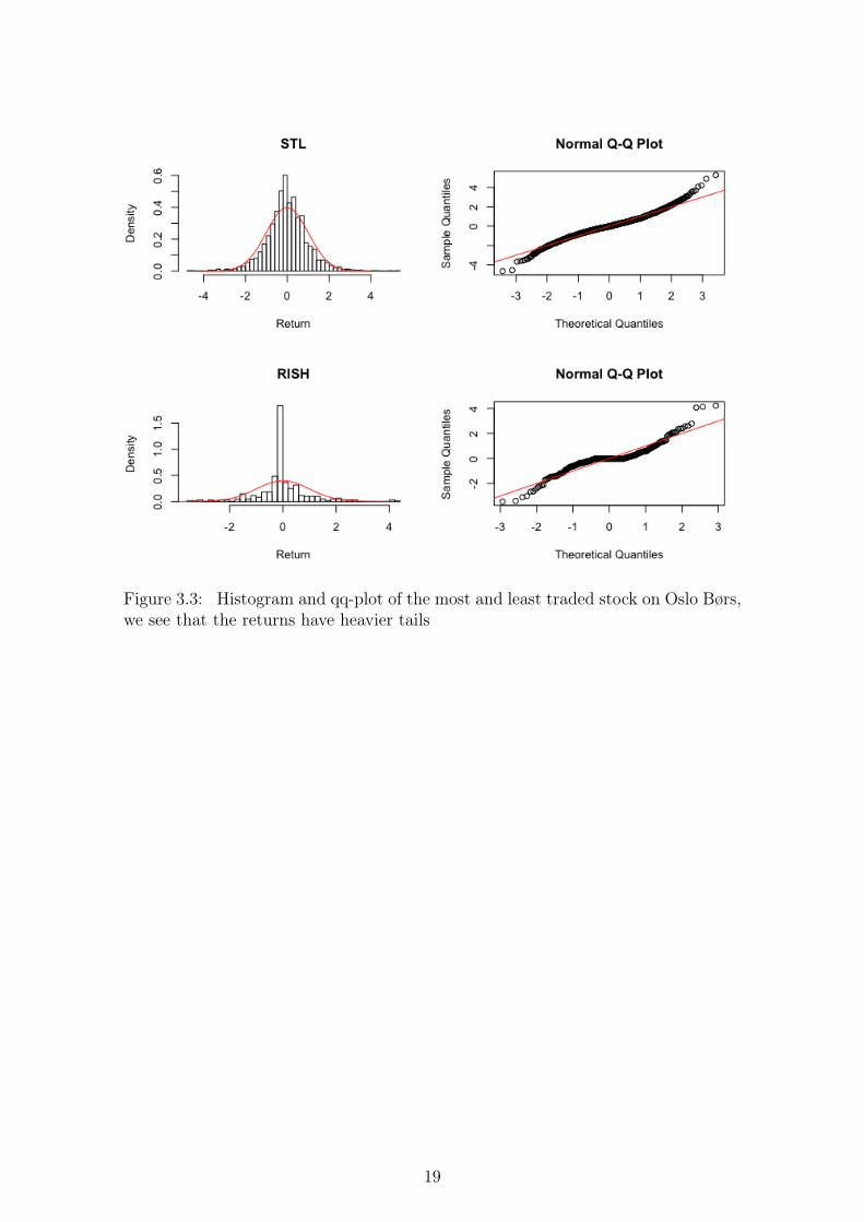
Figure 3.3: Histogram and qq-plot of the most and least traded stock on Oslo Børs,we see that the returns have heavier tails

19

Chapter 4

Covariance

4.1 The covariance matrixThe covariance matrix contains information about the pairwise dependence amongthe components of a random vector X, where X = (X1, ..., XP )T is a P-dimensionalrandom vector with the mean vector µ = E(X) = (µ1, ..., µP )T .

The covariance matrix Σ is defined as a p× p matrix

COV (X) = Σ = E((X − µ)(X − µ)T ))

Where COV (Xi, Xj) = Σij = E((Xi − µi)(Xj − µj))). The covariance matrix, Σ ispositive-semidefinite and symmetric matrix. In mean-variance framework it is alsoassumed that Σ is positive-definite, since we require invertibility. For some basicproperties of the covariance matrix I refer to [8]

4.2 Estimation errorMarkowitz’s framework assumes known µ and Σ, but in practice µ and Σ are un-known and has to estimated from historical data or expectations about the future.This means that precision of these estimates is uncertain and estimation error canbe made.

A survey done by DeMiguel et al. (2007)[9] found that none of the various mean-variance portfolios with different mean and covariance estimates in the survey wasable to significantly or consistently outperform the simple equally weighted 1/Nportfolio. The authors explained the poor performance of the portfolios relative tothe equally weighted portfolio was due to estimation error. It is shown that mean-variance portfolios are highly sensitive to estimates of means and covariance andsmall changes to these inputs result in extremely different portfolios[10], these prob-lems have caused mean-variance optimization to not bee used directly in practice.The sensitivity has been credited to the optimization frameworks ability to magnifythe effects of estimation error and for this reason, Michaud [11] has referred to meanvariance portfolio optimization as error maximization. It is also known that it is

20

more difficult to estimate means than covariances of asset returns, and that errorsin estimates of the means have a bigger impact on portfolio weights than of thecovariance matrix[12] and that the covariance matrix can be estimated much moreprecisely than the expected returns[13]. When the sample mean is used the estima-tion error may be so large not much is lost in ignoring the mean altogether[14]. Forthis reason, in order to decrease the estimation errors, we can avoid the estimationof expected returns and instead assume that all stocks have equal expected returns.This means that portfolios differ only with respect to risk, which means that theonly efficient portfolio will be the global minimum variance portfolio. The globalminimum variance portfolio is appealing since the portfolio weights are only deter-mined by the covariance matrix, or more accurately of its inverse, and not the means.

Assumption: We will in this thesis assume that expected returns are all equaland µ = 0, r ∼ N(0,Σ).

The covariance matrix is intuitively useful, to better understand the statistical re-lations between the data. However, computationally its inverse, often referred toas the precision matrix, Σ−1 is more relevant in the mean-variance optimizationframework. As stated the precision matrix is actually the only parameter computedto find the optimized weights for the global minimum variance portfolio, as we re-member the optimal solution of the global minimum variance problem is given by,wgmv = Σ−1e

eTΣ−1e. Since the real inverse is unknown it has to be estimated from data,

and so Σ−1 and must be replaced with an estimate Σ−1, which gives the estimatedweights wgmv = Σ−1e

eT Σ−1e.

The traditional estimator of wgmv is constructed by using the sample covariancematrix Σ−1 = S−1. The traditional estimator is not a bad choice if the numberof assets P is significantly smaller than the number of observations N . But whennumber of assets P is in the same order as to the sample size N , P

N∼ 1 or larger

PN> 1 the estimate tends to be far from the population covariance matrix, and is

therefore not an appropriate estimator of Σ[15]. Several alternative estimators havebeen proposed in the literature to overcome the deficiencies of the sample matrix,some authors have proposed imposing some structure on the covariance matrix withfactor models[16]. Others have suggested shrinking the sample matrix toward a tar-get matrix[17] and some have used random matrix theory to correct the eigenvaluesof the sample matrix[15], see [18][19] for overview of different methods. Surprisinglymost of the research focuses on estimating Σ and not Σ−1, I only found two articles[19][20] addressing the inverse matrix when estimating GMVP. So in this thesis Iwill look at estimation methods for Σ−1 and how it will effect the global minimumvariance portfolio.

The main focus of this thesis will be to find a way to estimate global minimum vari-ance portfolio which gives better performance than the equally weighted portfolioand the portfolio constructed from the sample covariance matrix. The performancemeasure that will be used is out-of-sample variance of the portfolio, which is theportfolio variance in the next period.

21

4.2.1 Sample covariance matrixThe classical estimator of the covariance matrix Σ is the sample covariance matrix,S. Given N observations of a P dimensional random vector X = (X1, ....XP )T , Wedefine the sample covariance as

S =1

N − 1

N∑t=1

(Xt − X)(Xt − X)T

where X = 1n

∑nt=1Xt. S has a number of advantages: it is simple to construct,

unbiased, and intuitively appealing[18]. But there are also several disadvantages.The obvious problem is that when the number of observations N is less than thenumber of variables P , then S is not invertible. But even when N is close to P ,PN∼ 1 , the sample covariance S has a significant amount of sampling error, and

its inverse is a poor estimator for Σ−1[18]. Under the normality assumption, theexpected value of the inverse is E(S−1) = n

n−p−2Σ−1. While S is unbiased for Σ,

S−1 is highly biased for Σ−1, if P is close to N [18]. We see that if P = N/2− 2, wehave E(S−1) = 2Σ−1.

4.3 Precision matrixThe precision matrix, Θ = Σ−1, has a specific mathematical interpretation. Theelements in Θ contains information about the partial correlation between variables.That is, the covariance between pairs i and j, conditioned on all other variables[21].One can think of this as a measure of how correlated two vectors are given the influ-ence of a set of other variables has been considered. An important result concerns ifthe vectors Xi and Xj are normally distributed, in which case a partial correlationof 0 implies conditional independence[21].

The precision matrix is closely related to the Gaussian graphical models, which isa framework for representing the structure of the conditional dependencies betweenGaussian random variables in a complex system. Graphical models provide an eas-ily understood way of describing and visualizing the relationships between multiplerandom variables. A Gaussian graphical model is an undirected graph G = (V,E)where the vertices(V ) represent the Gaussian variables and the edges(E) representthe dependencies between the variables. Estimating a Gaussian graphical model isequivalent to estimating a precision matrix[8]

4.4 EstimationGiven observations X1, X2...XN , Xi ∼ N(µ,Σ) which are i.i.d and comes from P-dimensional multivariate normal distribution. We would like to estimate Θ, one wayto do this is to through maximum likelihood estimation.

The log-likelihood of the data can be written as1

1When estimating with log-likelihood methods S will be denoted as S = 1N

∑Nt=1(Xt−X)(Xt−

X)T

22

l(Θ) = log(|Θ|)− trace(ΘS) (1)

Here we have ignored constants, and partially maximized with respect to µ, seeAppendix for more detail. |Θ| denotes the determinant of Θ.

The Θ that maximizes l(Θ) is S−1. And from theory, this maximum likelihoodestimate converges to the true precision matrix as the sample size N tends to infin-ity. But a problem arises when the number of variables P may be comparable to orlarger than the sample size N, in which case the MLE may be unstable or does notexist

4.4.1 RegressionThe entries of the precision matrix also has a regression-based interpretation[8]. Tosee this relationship between linear regression and the inverse covariance matrix, itis useful to partition the random variables X in two groups X = (Xi, X−i) whereX−i = (X1..., Xi−1, Xi+1, ...XP ) and express Σ as a block matrix.

Σ =

[Σii Σi−i

Σ−ii Σ−i−i

]Some useful identities about the entries in Θ are obtained by considering the linearleast-squares regression of Xi based on X−i,Xi = βiX−i + εi.

βi = Σi−iΣ−1−i−i

Θii = (Σii − βiΣ−ii)−1

Θi−i = −Θiiβi

From the identities we can express the inverse covariance matrix as

Θ =

[(Σii − βiΣ−ii)−1 −(Σii − βiΣ−ii)−1βi−βTi (Σii − βiΣ−ii)−1 Σ−1

−i−i + βTi (Σii − βiΣ−ii)−1βi

]=

[Θii −Θiiβi−βTi Θii Σ−1

−i−i + βTi Σ−1ii βi

]For more detailed derivation the reader is referred to the Appendix.

By changing i, the partition of X changes. Which means that we express eachrow or column of Θ by regression coefficient βi and the diagonal entry Θii. Fromthis we see that the sparsity of Θ is decided from the regression coefficients. Whichmeans that one cane develop methods to impose sparsity in the precision matrixfrom techniques devolved for linear regression.

4.4.2 SparsityA frequent task is statistics is to estimate the covariance matrix of a set of nor-mally distributed random variables from given samples, but in the high-dimensionalregime this is often a challenge and therefore it is important to have robust al-ternatives to the standard sample covariance matrix estimator. The principle ofparsimony(sparsity) is often used when developing methods for large covariance or

23

precision matrices estimation. The idea of an sparse precision matrix in covarianceestimation first appeared in the work of Dempsters in 1972[22], and numerous meth-ods for sparse precision matrix estimation have been developed since[23].

The reason to impose sparsity in precision matrix can come from either from apriori information about the variables or from estimation issues. If Θij = 0 thismeans that there is a conditional independence between variable j and i. i.e covari-ance between i and j is 0 when factoring in all other variables. For some types ofvariables the notion of conditional independence is natural, variables belonging to agiven class is likely to be related together while variables from different classes aremore likely to be independent. When the number of variables P is comparable toor larger than the sample size N , the sample estimate may be unstable or does notexist. To overcome the problems that occur in high dimensional setting, regular-ization is often used. Regularization means to impose a penalty on the estimatedparameters to control the magnitude of the parameters. When the L1 penalty isused, it will also promote sparsity.

If we know the structure of the graph, i.e which of the edges that are missing,which entries of Θ are zero. Then we could maximize (1) under the constraints thatparameters in Θ are zero. We will see that we can use the regression identities weintroduced earlier to solve for Θ and its inverse W = Θ−1, one row and column ata time.

To constrain the log-likelihood (1), we add Lagrange constants for all missing edges.

log(|Θ|)− trace(ΘS)−∑

(j,k)/∈E

γjkΘjk (2)

The gradient equation for maximizing (2) can be written as[21]

W − S − Γ = 0

Γ is a matrix of Lagrange parameters with nonzero values for all pairs with edgesabsent. From the gradient equation we get W−ii−S−ii−Γ−ii = 0. We also have therelationship W−ii = W−i−iβ

Ti such that

W−i−iβTi − S−ii − Γ−ii = 0 (3)

Now we can solve (3) by simple subset regression. Suppose there are p− q nonzeroelements in Γ−ii these correspond to the absent edges in node i. These p−q elementscarry no information, therefore we can reduce βi to β∗i by removing its p−q elementscorresponding to nonzero elements in Γ−ii. Yielding the reduced q × q system ofequations.

W ∗−i−iβ

T∗i − S∗−ii = 0

Which we can solve for β and gives βT∗i = W−1∗−i−iS

∗−ii, β∗i is then padded back with

p − q zeros to give β. This leads to the simple iterative procedure, where we canupdate W for each i, W−ii = W−i−iβ

Ti , it can be summarized as:

24

1. Initialize W = S

2. Until convergence2, Repeat for i = 1, 2.....P

(a) Partition W into part 1, (−i): all but the ith row and column, and part2, i: the ith row and column

(b) Set β∗i = W−1∗−i−iS

∗−ii. Where p − q elements corresponding to the zero

edges are removed. fill β∗i with p− q zeroes to get βi.

(c) Update W−ii = W−i−iβTi

3. For each i in the final cycle, set Θ−ii = βiWii−βiW−ii

For more details about this procedure see Appendix and [21]

4.4.3 Graphical lassoIn most cases we do not know which edges in the graph is zero. And so inferenceabout the structure of the graph has to be done. Meinshausen and Buhlmann[25]took a simple approach to the problem, rather than trying to fully estimate Θ, theyonly identified the nonzero entries of Θ. To do this, they fitted a lasso regressionusing each variable as the response and the others as predictors. Θij is estimated tobe zero if the regression coefficient for variable j in the lasso regression of variables−i on variable i, lasso(X−i, Xi), is zero and/or if the coefficient for variable i in theregression lasso(X−j, Xj) is zero. Banerjee et al.[26] and Yuan and Lin[27] providedfurther improvements of the initial work of Meinshausen and Buhlmann[25]. Inboth works, the problem of estimating Θ is seen as a penalized maximum likelihood.Instead of considering P different regression problems, the two articles focus on thelikelihood of the Gaussian variables and penalizes the entries of the concentrationmatrix with a L1 penalty.

log(|Θ|)− trace(SΘ)− λ ‖Θ‖1 (4)

Here λ is a penalty parameter which controls the amount of L1 penalty imposed,and ‖Θ‖1 is the sum of the absolute values of the elements. Friedman et al.[24] usedthis previous work as a launching point to propose a new algorithm that finds Θ thatmaximizes (4), which they called the graphical lasso. The graphical lasso (glasso)algorithm is very similar to algorithm in the previous section, but replaces step 2bwith a lasso problem. The reason for this is the gradient equation for maximizing(4) can be written as W − S − λSign(Θ)[21], which is equivalent with the gradientof a lasso problem, see the Appendix for the derivation. The glasso algorithm is:

1. Initialize W = S + λI

2. Until convergence, Repeat for i = 1, 2.....p

(a) Partition W into part 1(−i): all but the ith row and column, and part2(i): the ith row and column

(b) solve the lasso problem, minβ{12‖W

12−i−iβi −W

− 12

−i−iS−ii‖22 − λ‖βi‖1}

2convergense is defined as that the average absolute change in W is less than a certain value[24]

25

(c) Update W−ii = W−i−iβi

3. For each i in the final cycle, set Θ−ii = βiWii−βiW−ii

The solution glasso gives is positive definite Θ for all λ > 0 even if S is singular[28].If W−i−i = S−i−i in 2 b for every cycle, then the solutions of β would be equalthe lasso estimates for the ith variable on the others, such as in Meinshausen andBuhlmann approach [24]. In general W−i−i 6= S−i−i and therefore a P separate lassoregression as in the Meinshausen and Buhlmann[25] approach does not yield themaximum likelihood estimator.

26

Chapter 5

Sparsity structure

When we impose sparsity on precision matrix it is either that we think that thereexists some conditional independence in the data or to handle estimation problems.In our case it will be a mixture of both, since the data we are considering are stockreturns which can often be high dimensional, regularization can bu used to fix prob-lems such as invertibility of Σ. But it is also natural to think there exists groups ofstocks that are more similar than others, and that it exists conditional independencebetween pairs unsimilar stocks. One common way to think. is that stocks grouptogether is by industry affiliation, and most market agents assume that companieswithin industries are more tightly correlated than a random sample of companies[29].One way to describe the dependence structure of stocks is to characterize it with acommunity network structure. A graph is said to have community structure if thereare groups of nodes such that there is a higher density of edges within groups thanbetween them.

Figure 5.1: Example of a community structure graph

The principle in this kind of structure is that pairs of nodes are more likely to beconnected if they are both members of the same group(community), and less likelyto be connected if they do not in the same group. This implies that the graph willbe dense for nodes in the same group while being sparse in between nodes in dif-ferent groups. Many real world networks have community structures such as socialnetworks and biological networks, and it is intuitive to think stocks also exhibit thiskind of structure. Such that stocks for companies operating in the same industrywill be more likely to be connected then companies that are not in the same in-dustry. Some research of the community structure in financial markets has beendone, and it has been shown that correlation networks from stock returns exhibit

27

a community structure and the communities correspond the industrial classificationof the companies to some extent[30][31]

In this thesis we will assume that the data originates from a community struc-ture, and in all the simulations we will simulate from a community structure. I willin this chapter present how data for the simulations was generated

5.0.1 Graph GenerationIn the simulations in this thesis I will use a simple method for generating data thathas an underlying community structure. We will first generate the graph whichrepresent the structure of the data and then generate a Θ from this structure, thatcan be used to simulate data. I present here the method used for generating thegraph structure.

Given the inputs:

• P , number of nodes in the graph

• K, number of groups

• c, which will be vector of length P that represents each node group classifica-tion.

• Γ is a K×K symmetric matrix where Γii is the probability of an edge betweentwo nodes in the same group, and Γij is the probability of an edge betweentwo nodes in from group i and j.

we can generate an adjacency matrix. An adjacency matrix A is a P × P matrixwhich can be used to represent the structure of a graph. it is defined as

Aij=

{1 if i, j connected0 else

For undirected graphs A is symmetric.

Given a Γ we can randomly generate A, where Aij is 1 with probability Γkl wherenode i is in group k and node j is in group l. In this thesis we will operate withthe same inter and intra-group probabilities for all groups, this means Γii = p forall i ∈ 1, .., K and Γij = q for all i 6= j, and it will also be assumed p > q. Thisrandom graph structure is also known as Stochastic Block Model, with associativecommunities[32].

28

Figure 5.2: Generated community graphs with different inter and intra-group prob-abilities

In all the simulations we will use p = 1 and q = 0.1 for inter and intra-groupprobabilities, and the number of groups will be K = log(P ).

Figure 5.3: Generated community graphs when p = 1,q = 0.1, P = 50 andK = log(P )

29

5.0.2 Simulate from structureGiven an adjacency matrix A we want to simulate a N ×P data observation matrixO = (O1, ..., ON)T , where each observation Oi ∼ N(0,Σ) and Σ−1 = Θ has the samezero entries as A. To my knowledge there is no standard methods to generate aprecision matrices with a specified sparsity structure, therefore I propose my ownmethod.

The challenge is to get a positive definite matrix which has the same zero entries asA, since the adjacency matrix not necessarily positive definite we cannot just useΘ ◦ A as a new sparse precision matrix ΘA, where Θ is a arbitrary dense precisionmatrix and ◦ denote the Hadamard product.

For two matrices A,B of the same dimension N × P the Hadamard productA◦B is a matrix defined as the element wise product of A,B (A◦B)ij = AijBij

Notice that if A was positive definite then ΘA would also be positive definite by Schurproduct theorem[8]. So if we could find a matrix L that had the same structure as Aand is positive definite we would get our desired matrix ,ΘL. Finding such a L thathas the exactly same is not hard to find, one way to achieve this is to add to thediagonal of A such that it becomes positive definite. We see that we add a constantc to the diagonal of A, L = A+ cI then we shift the eigenvalues of A upwards withc

L = A+ cI = QΛQT + cQQT = Q(Λ + cI)QT

Where Q is a orthogonal matrix of the eigenvectors of A and Λ is a diagonal matrixof the eigenvalues of A, A+ cI will have the same eigenvectors as A but the eigen-vectors will be λi + c for i = 1, .., P where λi is the eigenvalues of A. Since we onlyhave changed the diagonal of A the off-diagonal will still be the same, this meansthat if A is not positive definite we can find a positive definite matrix L that has thesame off-diagonal elements as A by adding a constant c to the diagonal of A suchthat the eigenvalues of L = A+ cI will be non negative. If we choose c =| λmin | +εwhere ε > 0, we will achieve positive definiteness.

With the method described above to find a matrix that has the same sparsity pat-tern as an adjacency matrix A and a procedure to generate dense precision matrix,We can define a procedure for randomly generating data from underlying sparsestructure

Input: A

1. define L, L = A+ I(| λmin | +ε)

2. Generate Σ and calculate Σ−1 = Θ

3. Define ΘL = Θ ◦ L

4. Calculate ΣL, ΣL = Θ−1L

30

5. Generate O, O ∼ N(0,ΣL)

For the generation of the dense covariance matrix Σ the following method will beused:Generate P × K matrix W from N(0, 1) where K ≤ P and 1 × P vector d fromN(0, 1). Define V = WW T +D where D is diagonal matrix with d as the diagonal.Then normalize to a correlation matrix C = NVN where N is a diagonal matrixwith diagonal elements 1√

Viifor i = 1, ..P . And then rescale C to a covariance matrix

with your desired variance range, Σ = RCR where R is a diagonal matrix sampledfrom the range (0,

√σ) where σ is the desired maximum variance.

One thing worth noticing is that the choice of K controls the distribution rangeof the off diagonal elements of C and Σ, the lower the K the wider the range willbe. Which means that this generation method is suitable when you want some highcorrelations in the data. In all the simulations I will use K = 0.1

Figure 5.4: Distribution of the correlations for different K, in this plot P = 100

In many cases, such as in this thesis, you want to control the maximum varianceof ΣL. Since the interest is in stock returns, it is preferable that the simulated datareflects the nature of the returns, hence I would like to set a likely range for wherethe simulated returns fall in, from the return distribution chapter we saw that mostof the returns fall in the range (−0.1, 0.1). Controlling the range the returns willfall in is achieved by setting a maximum value for the variance in the covariancematrix, I will use some results from George P.H. Styan[33] to find out what to setthe maximum value for the variance in the covariance matrix ΣL.

When A and B are positive definite we have that

λmin(A)Bmin ≤ λi(A ◦B) ≤ λmax(A)Bmax

31

for i = 1, ..., P , where λmin and λmax is the smallest and largest eigenvalue and Bmin

and Bmax is the smallest and largest value of the diagonal of B. We also have whenA is symmetric λmin(A) ≤ Aii ≤ λmax(A) for i = 1, ..., P . From this we get

1

λmin(A)Bmin

≥ 1

λi(A ◦B)

λmax(A−1)

Bmin

≥ λi((A ◦B)−1)

max((A ◦B)−1ii ) ≤ λmax((A ◦B)−1) ≤ λmax(A−1)

Bmin

If we control the maximum eigenvalue of dense Σ in step 2 we can control the max-imum variance in ΣL since max((ΣL)ii) = max((Θ ◦ L)−1

ii ) ≤ λmax(Σ)Lmin

. If we set ourdesired maximum value of (ΣL)ii as η, we could achieve this by setting the maximumeigenvalue of Σ as Lminη.When we assume that our observations comes from a multivariate Gaussian distribu-tion, each of univariate variable has an univariate Gaussian distribution. The valuerange each of the univariate variable i is controlled by the variance (ΣL)ii, for anunivariate Gaussian variable the 68–95–99.7[34] rule states that values will lie within2σ range with a probability of approximately 95% and 3σ range with a probabilityof approximately 99.7%, where σ is the standard deviation. For the stock returnswe want most of the returns to fall in range (−0.1, 0.1), which we can achieve besetting the max variance η in the range ((0.1

2)2, (0.1

3)2). In the simulations I will use

η = (0.12.5

)2

32

Chapter 6

Tuning parameter

The graphical lasso solution of (4), log(det(Θ)) − trace(SΘ) − λ ‖Θ‖1, gives us aΘ per fixed λ, Θλ, so deciding an optimal λ for the glasso method has to be done.The penalty parameter λ controls the amount of L1 penalty imposed, which againcontrols the sparsity in Θλ. For small λ the solution of (4) will tend to be denseand in the case of λ = 0 we will get Θ0 = S−1. And as we increase λ the solution of(4) will tend to get more and more sparse, and eventually for a large enough λmax,where Θλmax will be a diagonal matrix. For determining λmax we can use the resultfrom banerjee et al. [26] that states

If λ ≥ |Sij| for all i 6= j then Θλij = 0 for i 6= j

From this result it can be seen that if λ = max(|Sij|) is chosen for i 6= j thenΘλmax will be a diagonal matrix, hence λmax = max(|Sij|) for i 6= j.

The existence of the penalty term λ is what encourages sparsity in the estimatedprecision matrix, and different λ will give different estimates if the precision matrixand different levels sparsity, which will give different portfolio weights, so finding themost optimal λ is therefore a crucial task when estimating Θ. I will discuss some ofthe methods developed for choosing λ.

6.0.1 MethodsUsually a method for choosing an optimal λ, (λopt) selects λ from a grid of val-ues Gλ = (λmin, ..., λmax) which maximizes/minimizes a score measuring the somegoodness-of-fit. Several model selection regimes is proposed in the literature suchas cross-validation, information criteria, stability-selection. In this chapter some ofthe methods from from the different regimes will be presented.

AIC

The Akaike information criterion(AIC) is based on estimating Kullback-Leibler di-vergence which characterize the information that is lost when approximating thetrue model[35]. AIC is defined as −2l(Θλ) + 2df(λ)[36] where l is the log likelihoodfunction and df is degrees of freedom of, which reflects model complexity. The modelpreferred in AIC selection is the one that minimizes the AIC value.

33

λAIC = minλ∈Gλ{−2l(Θλ) + 2df(Θλ)}

BIC

The Bayesian Information Criterion estimates the Bayes factor, which is a ratioof posterior probability between competing models[35]. It is defined as −2l(Θλ) +log(n)df(λ)[36], the model with the lowest BIC is likely to have the highest posteriorprobability, so the model preferred in BIC selection will be the model with the lowestBIC value[35].

λBIC = minλ∈Gλ{−2l(Θλ) + log(n)df(Θλ)}

In our graphical model setting the log likelihood l(Θ) is equal to −N2

(− log(|Θ|) +trace(ΘS)) up to a constant (see appendix), when selecting λAIC , λBIC . In graphicalmodel estimation it is common to define the degrees of freedom are defined asdf(Θλ) =

∑i≤j I(Θλij 6= 0)[37][27], which is the number of unique non zero elements

in the estimated precision matrix.The model selection criterion can then be written as

λAIC = minλ∈Gλ{−N log(|Θλ|) +Ntrace(ΘλS)) + 2∑i≤j

I(Θλij}

λBIC = minλ∈Gλ{−N log(|Θλ|) +Ntrace(ΘλS)) + log(N)∑i≤j

I(Θλij}

We see from the expressions of AIC and BIC that the difference between them inis how they penalize model complexity, the BIC penalizes model complexity moreheavily. This means that BIC will choose higher values of λ then AIC, which givessparser estimates of Θ.

AIC and BIC tend to perform poorly when the dimension is large relative to thesample size[38]. And when P > N the estimate the degree of freedom may even nothold[38]. To correct performance in high dimension the criterion called the extendedBIC (EBIC), was developed[39].

λEBIC = minλ∈Gλ{−2l(Θλ) + log(N)df(Θλ) + 4df(Θλ) log(P )γ}

γ ∈ (0, 1) For positive values of γ it was demonstrated that the EBIC lead toimproved graph inference when P and N are of comparable size[39], in this thesiswe will use γ = 1.

Cross-validation

Another commonly used method of model selection is cross-validation(CV). In data-rich situations, a good approach for model selection is to randomly divide the datasetinto three parts: a training set, a validation set, and a test set. The training set isused to fit the models, the validation set is used to evaluate the goodness-of-fit forthe models, the test set is used for assess the chosen model for unseen data. Manytimes there is not enough data available to partition it into three sets without losingsignificant modelling performance[21]. The main idea in CV is to split the data into

34

many a training and validation sets and then use the accumulated goodness-of-fitmeasure from all the validation sets as an estimate for the fit in the test data. Themodel with the best overall performance on the validation set is selected.

K-fold cross-validation

In K-fold cross-validation you randomly split your data into 1, ..., K almost equal-sized parts, and for each k ∈ K you use part k as validation set and K − 1 otherparts as a training set to fit your model. Splitting your data into 5 or 10 foldsis most commonly used[21] and when K = N the method is called leave-one-outcross-validation (LOOCV). The K-fold cross-validation score which will be used isdefined as[27]

CV (λ) =K∑i=1

− log(|Θλ,−k|) + trace(Θλ,−kSk))

Here Sk is the sample covariance matrix of data from fold k and Θλ,−k is the es-timated precision matrix from k − 1 other folds, K = 5 will be used. The cross-validation score is based on the Kullback-Leibler divergence between the trainingand validation set[40].

StARS

Stability Approach to Regularization Selection (StARS)[38] is a more recent devel-oped model selection approach compared to the others, in StARS the goal is toachieve model stability. The idea of the approach is to randomly draw subsam-ples(can be overlapping) from the data and construct a graph from each sample, wethen select the model based on which graphs that are sparse and do not have not toomuch variability across them. More precisely, we start with a large regularizationλmax which corresponds to an empty(stable) graph and then gradually reduce λ untilthere is a small but acceptable amount of variability of the graph across subsamples.

The selection method goes as following: Start with selecting a sampling size bwhere b < N , and then sample n samples without replacement S1..., Sn fromX = (X1, ...XN) where each Si is of length b. Then for each λ define the adja-cency matrix Aλ(Si) for each i ∈ (1, n) where Aλ(Si) is the adjacency matrix ofthe precision matrix generated from the sample Si. Then for each edge in Aλ(Si)define ξij(λ) = 2ζij(λ)(1− ζij(λ)) where ζij(λ) = 1

n

∑nk=1 Aλ(Sk)ij. Here ζij(λ) is an

estimate of the probability of an edge between node (i, j) given a λ, and ξij(λ) ismeasure of how often the graphs of Aλ(Si) for i = 1, .., n disagree on estimating anedge between node (i, j). The selection criterion will then be defined as the averageinstability of all the nodes.

StARS(λ) =∑i<j

ξij(λ)(Nk

)StARS(λmax) will be close to 0 since Aλmax(Si) will usually be close to a diagonal

matrix, and StARS(λ) will increase as λ decreases until λ becomes so low thatAλ(Si) becomes dense such that StARS(λ) will start to decrease. StARS aims to

35

find a sparse graph where the instability is at a specified value β. The selectedmodel will be selected after the criterion:

inf{λ : StARS(λ) < β}

where StARS(λ) = supλ<t<λmaxStARS(t).

The interpretation of the criterion is that we select the densest of the sparsestgraphs that is in line with our β, even though the StARS replaces the problem ofchoosing λ with the problem of choosing β Liu et al.[38] argues that β is an inter-pretable quantity and sets a default value for β = 0.5, they also suggested the valueb = n

√10 for sampling size, I will use the same values and n = 20.

If the goal is graph inference then the criteria BIC, EBIC and StARS are pre-ferred, while using cross-validation and AIC will result with a model with a goodpredicting power, in the sense that we can get Θ estimate that are close to the trueΘ in Kullback-Leibler divergence[40].

6.0.2 Predicting power vs graph recovery

The application for Θ in this thesis is to construct portfolio weights w(Θ) = Θe

eT Θewhich are close to true weights wΘ, so we are more likely to be interested in predict-ing power over graph recovery. To find out which model selection regime is mostsuited for our problem I will do a simple simulation experiment.

Given a N×P data matrix O of which is generated from a known Θtrue we would liketo find out if methods that focus on graph recovery or Kullback-Leibler divergencegives the best results for finding optimal portfolio weights. To determine this I willdo the following simulation experiment.

1. Generate an adjacency matrix A, which is described in the graph generationchapter.

2. Given A, we can generate Θtrue and Σtrue. When we have the Σtrue we cansimulate O from N(0,Σtrue), this is described in simulate from structure chap-ter

3. From O we can use the glasso algorithm to solve (4) for different λ ∈ Gλ

4. For the estimated Θλ for each λ ∈ Gλ we select λ after two different criteria.One that focuses on graph recovery and one that focuses on Kullback-Leiblerdivergence.

5. After deciding the two λ,(λF1 ,λKL), we get the two estimated precision matri-ces ΘF1 ,ΘKL. We then calculate the weights w(ΘF1) and w(ΘKL) given by thetwo matrices.

6. We then compare the weights to the weights obtained from Θtrue, w(Θtrue).

36

7. This procedure is repeated T times and for different N and a fixed P , and welook at the average different P

Nto evaluate which selection regime that gives

the best result.

The F1 score will be used as criterion to find the Θλ which has a graph structureclosest to the true graph of Θtrue, The F1 scores is defined as

F1 =2TP

2TP + FN + FP

where TP, FN, FP is the number of true positives,false negative,false positives be-tween Θtrue and Θλ. The F1 score measures the quality of a binary classifier, it canbe seen as a weighted average of the specificity( TP

TN+FP) and specificity( TP

TN+FN), the

F1 score reaches its best value at 1 and worst at 0. The λ corresponding to highestF1 score will be chosen, λF1 = maxλ∈Gλ{F1(λ)}, which gives ΘF1 .

The second criterion finds the λ, such that Θλ has the smallest Kullback-Leiblerdivergence. Kullback-Leibler divergence for graphical models are defined as[40]

KL =1

2(− log(det(Θ−1

trueΘλ)) + trace(Θ−1trueΘλ)− P )

We choose the λ that minimizes the Kullback-Leibler divergence λKL = minλ∈Gλ{KL(λ)},which gives us ΘKL

We then calculate the weights w(ΘF1) =ΘF1e

eTΘF1eand w(ΘKL) = ΘKLe

1TΘKLeand compare

them to weights obtained from w(Θtrue) = ΘtrueeeTΘtruee

by calculating the distances.

DF1 =P∑i=1

(wi(Θtrue)− wi(ΘF1))2

DKL =P∑i=1

(wi(Θtrue)− wi(ΘKL))2

In the experiment conducted I compute DF1 and DKL for P = 50 and N =(100, 90, 80, 70, 50, 50, 40). And repeat 100 times T = 100, the average DF1 andDKL are reported below.

37

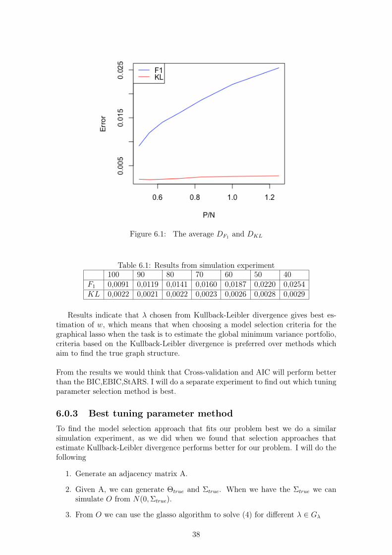
Figure 6.1: The average DF1 and DKL

Table 6.1: Results from simulation experiment100 90 80 70 60 50 40

F1 0,0091 0,0119 0,0141 0,0160 0,0187 0,0220 0,0254KL 0,0022 0,0021 0,0022 0,0023 0,0026 0,0028 0,0029

Results indicate that λ chosen from Kullback-Leibler divergence gives best es-timation of w, which means that when choosing a model selection criteria for thegraphical lasso when the task is to estimate the global minimum variance portfolio,criteria based on the Kullback-Leibler divergence is preferred over methods whichaim to find the true graph structure.

From the results we would think that Cross-validation and AIC will perform betterthan the BIC,EBIC,StARS. I will do a separate experiment to find out which tuningparameter selection method is best.

6.0.3 Best tuning parameter methodTo find the model selection approach that fits our problem best we do a similarsimulation experiment, as we did when we found that selection approaches thatestimate Kullback-Leibler divergence performs better for our problem. I will do thefollowing

1. Generate an adjacency matrix A.

2. Given A, we can generate Θtrue and Σtrue. When we have the Σtrue we cansimulate O from N(0,Σtrue).

3. From O we can use the glasso algorithm to solve (4) for different λ ∈ Gλ

38

4. For the estimated Θλ for each λ ∈ Gλ we select λ after the AIC,BIC,EBIC,StARSand CV criteria.

5. After deciding λ after the different criteria, λAIC , λBIC , λEBIC , λStARS, λCV ,we get the estimated precision matrices ΘF1 ,ΘBIC ,ΘEBIC ,ΘStARS,ΘCV . Wethen calculate the weights w(ΘM) M ∈ AIC,BIC,EBIC, StARS,CV givenby the matrices.


7. We also select one λ that minimizes the distance between w(Θtrue) and w(Θλ)for λ ∈ Gλ, which we will call Oracle and use it as reference.

λOracle = minλ∈Gλ

{P∑i=1

(wi(Θtrue)− wi(Θλ))2}



the best result.

They way we compare the weights is by using the distance

DM =P∑i=1

(wi(Θtrue)− wi(ΘM))2

where M ∈ AIC,BIC,EBIC, StARS,CV .In the experiment conducted I computeDM and for P = 50 andN = (100, 90, 80, 70, 50, 50, 40).And repeat 100 times T = 100, the average DM are reported below.

Figure 6.2: The average DM for each method, for different PN,P = 50 ans T = 100

39

Table 6.2: DM for the different methods when,P = 50 ans T = 100100 90 80 70 60 50 40

Oracle 0,0046 0,0052 0,0051 0,0065 0,0068 0,0069 0,0075AIC 0,0066 0,0074 0,0064 0,0081 0,0082 0,0137 0,0313BIC 0,0079 0,0091 0,0080 0,0094 0,0093 0,0094 0,0093EBIC 0,0088 0,0104 0,0091 0,0105 0,0105 0,0107 0,0109StARS 0,0103 0,0118 0,0105 0,0121 0,0119 0,0118 0,0117CV 0,0069 0,0077 0,0071 0,0084 0,0084 0,0085 0,0084

From this result we see that cross-validation gives us the best overall results. Theresult are also in line with our previous findings that methods based on Kullback-Leibler divergence will give us the best weights, except for AIC when P

N≥ 1 then

the AIC seem to perform poorly.

Due to computational time P = 50 was chosen, since the generality of the resultsshould hold for all dimensionalities I will conduct the same experiment on a smallerscale with increased P , to see if the results can be generalized. I compute DM andfor P = 100 and N = (200, 100, 50). And repeat 10 times T = 10, the average DM

are reported below.


40

Table 6.3: DM for the different methods when,P = 100 ans T = 10200 100 50

Oracle 0,0028 0,0035 0,0033AIC 0,0033 0,0037 0,0108BIC 0,0036 0,0039 0,0035EBIC 0,0038 0,0043 0,0042StARS 0,0041 0,0049 0,0042CV 0,0033 0,0036 0,0034

Here we see that we can draw the same conclusions as in the previous experiment.Based on these results I will use cross-validation for choosing λ in further analysis.

41

Chapter 7

Experimental Results

In this section I want to provide some empirical evidence of the of the usefulnessof the glasso method for estimating the precision matrix when finding the globalminimum variance portfolio and compare them to the equally weighted portfolioand the traditional sample estimator. I first conduct an experiment on syntheticallygenerated stock data and then on data collected from actual stock prices.

7.0.1 Simulated dataFor simulated data we know the underlying generating parameters for the dataΣtrue and Θtrue, we can therefore check how well different methods estimate thetrue parameters. I will do this by comparing the estimated weights of the globalminimum variance portfolio to the weights given by the true parameter Θtruei n thefollowing way:

1. Generate an A.

2. Given A, we can generate Θtrue and Σtrue. When we have the Σtrue we cansimulate O from N(0,Σtrue).

3. From O we can use the glasso algorithm to solve (4) for λ = λCV and we cancalculate the sample covariance matrix S

4. Given the estimated precision matrices S−1,Θglasso, we calculate the weightsw(S−1) and w(Θglasso). We also define w(I) as the equally weighted weightsw(I) = ( 1

P, ...., 1

P)




the best result.

When P > N the sample precision matrix S−1 is not defined, here I will useMoore–Penrose pseudoinverse[41] instead when S−1 is not defined. And the dis-tance DM =

∑Pi=1(wi(Θtrue) − wi(ΘM))2 M ∈ S−1,Θglasso, I will still be used to

compare the weights.

42

In the experiment conducted I computeDM and for P = 50 andN = (100, 90, 80, 70, 50, 40).And repeat 100 times T = 100, the average DM are reported below.


Table 7.1: DM for each method, P = 50 ans T = 100100 90 80 70 60 50 40

Sample 0,7773 0,8734 0,9964 1,2395 1,7412 4,2231 1,80631/P 0,4470 0,4393 0,4500 0,4551 0,4424 0,4473 0,4537Glasso 0,2347 0,2401 0,2441 0,2620 0,2659 0,2639 0,2915

To validate the generality of the results I compute DM and for P = 100 andN = (200, 180, 160, 140, 100, 80). And repeat 10 times T = 10, the average DM arereported below.


43

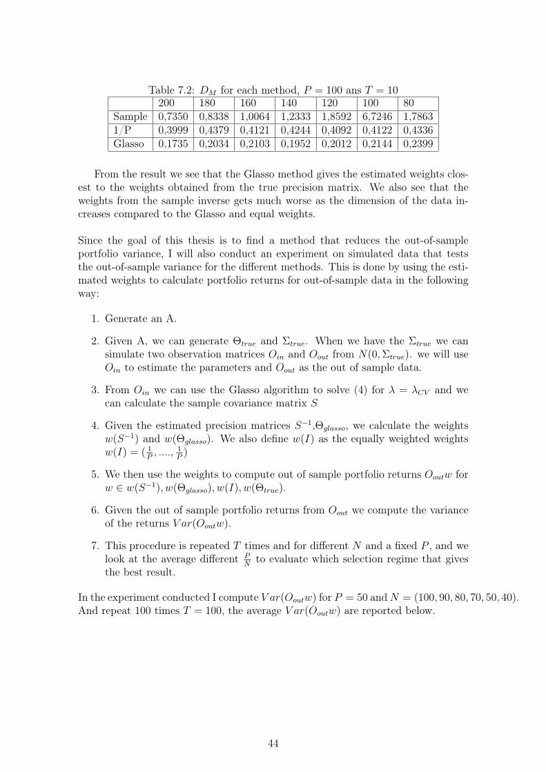
Table 7.2: DM for each method, P = 100 ans T = 10200 180 160 140 120 100 80

Sample 0,7350 0,8338 1,0064 1,2333 1,8592 6,7246 1,78631/P 0,3999 0,4379 0,4121 0,4244 0,4092 0,4122 0,4336Glasso 0,1735 0,2034 0,2103 0,1952 0,2012 0,2144 0,2399

From the result we see that the Glasso method gives the estimated weights clos-est to the weights obtained from the true precision matrix. We also see that theweights from the sample inverse gets much worse as the dimension of the data in-creases compared to the Glasso and equal weights.

Since the goal of this thesis is to find a method that reduces the out-of-sampleportfolio variance, I will also conduct an experiment on simulated data that teststhe out-of-sample variance for the different methods. This is done by using the esti-mated weights to calculate portfolio returns for out-of-sample data in the followingway:

1. Generate an A.

2. Given A, we can generate Θtrue and Σtrue. When we have the Σtrue we cansimulate two observation matrices Oin and Oout from N(0,Σtrue). we will useOin to estimate the parameters and Oout as the out of sample data.

3. From Oin we can use the Glasso algorithm to solve (4) for λ = λCV and wecan calculate the sample covariance matrix S

4. Given the estimated precision matrices S−1,Θglasso, we calculate the weightsw(S−1) and w(Θglasso). We also define w(I) as the equally weighted weightsw(I) = ( 1

P, ...., 1

P)

5. We then use the weights to compute out of sample portfolio returns Ooutw forw ∈ w(S−1), w(Θglasso), w(I), w(Θtrue).

6. Given the out of sample portfolio returns from Oout we compute the varianceof the returns V ar(Ooutw).



the best result.

In the experiment conducted I compute V ar(Ooutw) for P = 50 andN = (100, 90, 80, 70, 50, 40).And repeat 100 times T = 100, the average V ar(Ooutw) are reported below.

44

Figure 7.3: The average out-of-sample variance for each method, for differentPN,P = 50 ans T = 100

Table 7.3: Out-of-sample standard deviation for each method, P = 50 ans T = 100100 90 80 70 60 50 40

True 0,00297 0,00298 0,00294 0,00298 0,00290 0,00302 0,00305Sample 0,00418 0,00448 0,00493 0,00582 0,00727 0,02078 0,007521/P 0,00339 0,00338 0,00336 0,00338 0,00329 0,00342 0,00345Glasso 0,00308 0,00310 0,00307 0,00311 0,00303 0,00316 0,00320

I also computed V ar(Ooutw) for P = 100 and N = (200, 180, 160, 140, 100, 80).repeated 10 times and averaged.

Figure 7.4: The average out-of-sample variance for each method, for differentPN,P = 100 ans T = 10

45

Table 7.4: Out-of-sample standard deviation for each method, P = 100 ans T = 10200 180 160 140 120 100 80

True 0,00203 0,00205 0,00195 0,00200 0,00205 0,00206 0,00203Sample 0,00276 0,00306 0,00331 0,00377 0,00505 0,01389 0,005451/P 0,00230 0,00232 0,00227 0,00226 0,00238 0,00237 0,00236Glasso 0,00208 0,00210 0,00201 0,00205 0,00213 0,00215 0,00209

The result indicates that the Glasso method gives lower out-of-sample comparedto the equally weighted portfolio and sample estimator method. We can now moveon to testing on real data.

7.0.2 Real dataThe real world data collected in this thesis are stock returns from the Norwegianstock market traded on Oslo Børs. The data matrix containing the returns will bedenoted as R, I have collected daily geometric returns for 190 stocks ,P = 190 for1674 days, which i will denote as T = 1674. For the analysis of the out-of-sampleportfolio variance for the different methods I will use a rolling-window approach,this means to compute parameter estimates over a rolling window of a fixed sizethrough the sample. For each day t, the precision matrix and portfolio weightsare estimated using the N previous days from t − N to t, starting at day t =N + 1. The portfolio weights for the different methods are calculated for the periodt, wt(S−1), wt(Θglasso), wt(I) and the out-of-sample portfolio return for the next day(t+1) while holding the weights calculated in at t is calculated Rt+1wt. This processis continued by moving one day ahead for t ∈ N + 1, ...., T − 1, which gives us(T − 1)− (N + 1) out-of-sample sample returns. The variance of the out-of-samplesample returns for the different method is then calculated to infer which methodgives to lowest variance. The estimation period length I will use in this analysis isN = 100. The analysis will be done in the following way:

1. From R, select the subset R[t−N :t]

2. For R[t−N :t] we can use the glasso algorithm to solve (4) for λ = λCV and wecan calculate the sample covariance matrix S

3. Given the estimated precision matrices S−1, Θglasso, we calculate the weightswt(ΘS−1) and wt(Θglasso). We also define wt(I) as the equally weighted weightswt(I) = ( 1

P, ...., 1

P)

4. Given the estimated weights we can calculate the out-of-sample portfolio re-turn, Rt+1wt for wt ∈ wt(S−1), wt(Θglasso), wt(I)

5. This procedure is repeated for t+ 1 until t = T − 1

6. When all the wt are estimated and the put-of-sample returns are obtained, thevariance of each out-of-sample portfolio return series is calculated.

46

Missing values

When dealing with real stock data you may encounter that the prices is missingfor a certain days, and therefore no return. There are mainly two reasons for this,either the stock was not listed at the exchange at the time and was introduced ata later time. Or the stock was not traded that day, and hence no price was giventhat day. I will handle missing values in the following way

1. For each rolling window R[t−N :t], find the stock returns which have more than10% missing values. Remove these stock from R[t−N :t], this mean you cannotinvest in the stocks at time t.

2. For the stocks that has missing values below 10%, replace the missing valueswith the mean value.

There are several practices for dealing with missing values, this method is verysimple, for more sophisticated approaches see [42][43]. Due to missing values thenumbers of stocks the investor can invest in P may vary, such that P/N will varyfor different t. For P

N> 1 the Moore–Penrose pseudoinverse[41] will be used instead

of of the sample inverse. Below you can see a plot of the P used at each window.

Figure 7.5:

From this plot we see that the PN

range will be in (0.8, 1.5). The result of therolling-window analysis is reported in the table below in terms of the standarddeviations of the portfolio return.

Table 7.5: standard deviations of the out-of-sample portfolio returnMethod SDSample 0.00991/P 0.0108Glasso 0.0027

We see that the graphical lasso method gives considerably lower out-of-samplevariance compared to the two other methods. This can also be graphically illustratedby plotting all the returns from the different methods.

47

Figure 7.6: Portfolio returns for the different methods

Figure 7.7: Box plot of the returns for the different methods

From the figure we see that the range of the returns from graphical lasso estima-tion is smaller than of the sample and equally weighted estimates. If we comparethe result of the real data with the simulated data, we see that results agrees thatthe glasso method gives the best result. But we also see that the performance of theequally weighted gets worse for the real data. In the simulations the out-of-samplevariance of the glasso and the 1/P portfolio was of the same size, while for the real

48

data the sample and 1/P portfolio was of the same size. One possible explanationfor the decrease in the performance of the equally weighted performance is the non-normality of the actual stock returns, which gives more extreme returns than in thesimulations. Holding high variance stocks the 1/P portfolio will now give more ex-treme returns then in the simulations, while for the covariance based portfolios theweight will usually be lower than 1/P and therefore do not have the same decreasein performance.

Given the evidence from the simulated and real data, we can conclude that es-timating the inverse covariance matrix using graphical lasso method gives lowerout-of-sample variance for the global minimum variance portfolio. Compared to us-ing traditional sample estimate and investing equally in all assets.

As mentioned earlier several alternative estimators have been proposed in the lit-erature to overcome the deficiencies of the sample matrix. I will compare the per-formance of the graphical lasso against a method proposed by Olivier Ledoit andMichael Wolf[17], which has been shown to significantly lower out-of-sample vari-ance. The Ledoit&Wolf estimator is a shrinkage estimator, it is convex linear com-bination of the sample covarince matrix and a highly structured estimator, denotedby F .

ΣLW = αS + (1− α)F

Here α is called the shrinkage constant, and is always between 1 and 0. Ledoit &Wolf showed that using the identity matrix or a single-factor matrix as the shrinkagetarget F outperformed several other methods including the sample estimator, wherethe usage of a single-factor matrix gave best results. I will use a constant correlationmodel for F , as suggested Ledoit & Wolf in a later paper[44]. F is a matrix with thesame diagonal elements as S, but assumes that the off-diagonal elements have thesame correlation Fij = ρ

√SiiSjj, where ρ is the average sample correlation. It was

shown[44] that a constant correlation model for F gives comparable performance tothe single-factor model while being easier to implement. For more details of thismethod and the determination of α I refer the reader to [44][17]. The implementa-tion of this method for this thesis is done with the R-package "tawny".

I will use the same rolling-window approach on the real stock data to comparethe graphical lasso method and the Ledoit & Wolf method. Where Σ−1

LW will beused as the estimate of the precision matrix for the Ledoit & Wolf method. Theresults are presented in the table below.

Table 7.6: Standard deviations of the out-of-sample portfolio returnMethod SDGlasso 0.0027L&W 0.0060

49

Figure 7.8: Box plot of the returns for the two methods

We see that the glasso method give better performance than the shrinkagemethod by Ledoit & Wolf in terms of the out-of-sample variance.

50

Chapter 8

Concluding remarks

In this thesis I have used the graphical lasso method that was originally used to es-timate sparse undirected graphical models, to estimate the asset allocation weights.The motivation to employ this method came from the desire to reduce the errorassociated with the sample estimator when the number of variables are comparableto or larger than the sample size. And the connection between sparsity of the inversecovariance matrix and condition independence, which is intuitively appealing due tothe nature of financial assets. I have developed a method to simulate variables thatcan be represented from a sparse graphical structure and determined what kind oftuning parameter selection method is best suited for the graphical lasso when thedata stems for this structure, when the goal is portfolio variance minimization. It isshown though simulation and real world data analysis that the the graphical lassogives portfolios which has smaller out-of-sample variance than the traditional sam-ple estimator. It is also shown that the graphical lasso gives better performancethan portfolios using equal investment weights and existing shrinkage estimatorsdeveloped for portfolio selection.

8.1 Further researchAs some focus has been made on the group structure assumption of stocks, a naturalextension of this analysis is to investigate if using a-priori information about thenetwork structure of the variables can give better results. For real word stock datasuch prior knowledge can be the industry affiliation, Oslo Børs uses the GlobalInsustry Classification Standard (GICS) for grouping of companies. And since thesimulation methodology for grouped structure is already made experimentation caneasily be done. The challenge here is to extend the graphical lasso to incorporatestructure knowledge, such that the sparsity imposed in the methods follows the apriori structural information.

51

Bibliography

[1] H. Markowitz, “Portfolio selection*,” The Journal of Finance, vol. 7, no. 1,p. 77–91, 1952.

[2] R. S. A. of Sciences, “The prize in economics 1990 - press release.”http://www.nobelprize.org/nobel_prizes/economic-sciences/laureates/1990/press.html.

[3] A. O. Petters and X.-Y. Dong, An introduction to mathematical finance withapplications: understanding and building financial intuition. Springer, 2016.

[4] A. Beste, D. Leventhal, J. Williams, and Q. Lu, “The markowitz model selectingan efficient investment portfolio,” Lafayette College, 2002.

[5] K. Aas, “To log or not to log: The distribution of asset returns,” SAMBA/03/04,sep 2004.

[6] F. Black and M. Scholes, “The pricing of options and corporate liabilities,”Journal of Political Economy, vol. 81, no. 3, pp. 637–54, 1973.

[7] T. L. Lai and H. Xing, Statistical models and methods for financial markets.Springer, 2011.

[8] M. Pourahmadi, High-dimensional covariance estimation. Wiley, 2013.

[9] V. Demiguel, L. Garlappi, and R. Uppal, “Optimal versus naive diversifica-tion: How inefficient is the 1/nportfolio strategy?,” Review of Financial Studies,vol. 22, p. 1915–1953, Mar 2007.

[10] V. K. Chopra and W. T. Ziemba, “The effect of errors in means, variances, andcovariances on optimal portfolio choice,” The Journal of Portfolio Management,vol. 19, no. 2, p. 6–11, 1993.

[11] R. O. Michaud, “The markowitz optimization enigma: Is ‘optimized’ optimal?,”Financial Analysts Journal, vol. 45, no. 1, p. 31–42, 1989.

[12] V. Demiguel, L. Garlappi, F. J. Nogales, and R. Uppal, “A generalized ap-proach to portfolio optimization: Improving performance by constraining port-folio norms,” Management Science, vol. 55, no. 5, p. 798–812, 2009.

[13] A. Kempf and C. Memmel, “On the estimation of the global minimum vari-ance portfolio,” CFR Working Papers 05-02, University of Cologne, Centre forFinancial Research (CFR), 2005.

52

http://www.nobelprize.org/nobel_prizes/economic-sciences/laureates/1990/press.html

http://www.nobelprize.org/nobel_prizes/economic-sciences/laureates/1990/press.html

[14] R. Jagannathan and T. Ma, “Risk reduction in large portfolios: Why imposingthe wrong constraints helps,” Working Paper 8922, National Bureau of Eco-nomic Research, May 2002.

[15] H. Li, Z. D. Bai, and W.-K. Wong, “High dimensional global minimum varianceportfolio,” mpra paper, University Library of Munich, Germany, 2015.

[16] J. Fan, Y. Liao, and M. Mincheva, “High-dimensional covariance matrix esti-mation in approximate factor models,” Ann. Statist., vol. 39, pp. 3320–3356, 122011.

[17] O. Ledoit and M. Wolf, “Improved estimation of the covariance matrix of stockreturns with an application to portfolio selection,” Journal of Empirical Fi-nance, vol. 10, no. 5, pp. 603–621, 2003.

[18] J. Bai and S. Shi, “Estimating high dimensional covariance matrices and itsapplications,” tech. rep., Columbia University Academic Commons, 2011.

[19] M. Senneret, Y. Malevergne, P. Abry, G. Perrin, and L. Jaffres, “Covarianceversus precision matrix estimation for efficient asset allocation,” J. Sel. TopicsSignal Processing, vol. 10, no. 6, pp. 982–993, 2016.

[20] A. Kourtis, G. Dotsis, and R. N. Markellos, “Parameter uncertainty in portfo-lio selection: Shrinking the inverse covariance matrix,” Journal of Banking &Finance, vol. 36, no. 9, pp. 2522–2531, 2012.

[21] T. Hastie, R. Tibshirani, and J. Friedman, The Elements of Statistical Learning.Springer Series in Statistics, New York, NY, USA: Springer New York Inc., 2001.

[22] A. M. Dempster, “Covariance selection,” Biometrics, vol. 28, pp. 157–175, 1972.

[23] J. Fan, Y. Liao, and H. Liu, “An overview of the estimation of large covarianceand precision matrices,” The Econometrics Journal, vol. 19, no. 1, pp. C1–C32,2016.

[24] J. Friedman, T. Hastie, and R. Tibshirani, “Sparse inverse covariance estimationwith the graphical lasso,” Biostatistics, vol. 9, pp. 432–441, 2008.

[25] N. Meinshausen and P. Bühlmann, “High-dimensional graphs and variable se-lection with the lasso,” Ann. Statist., vol. 34, pp. 1436–1462, 06 2006.

[26] O. Banerjee, L. El Ghaoui, and A. d’Aspremont, “Model selection throughsparse maximum likelihood estimation for multivariate gaussian or binarydata,” J. Mach. Learn. Res., vol. 9, pp. 485–516, June 2008.

[27] M. Yuan and Y. Lin, “Model selection and estimation in the Gaussian graphicalmodel,” Biometrika, vol. 94, no. 1, pp. 19–35, 2007.

[28] D. M. Witten, J. H. Friedman, and N. Simon, “New insights and faster com-putations for the graphical lasso,” Journal of Computational and GraphicalStatistics, vol. 20, no. 4, pp. 892–900, 2011.

[29] G. Horrell and R. Meraz, “Test-driving industry classifications,” tech. rep., Jour-nal of Indexes, 2009.

53

[30] S. Wu, M. Tuo, and D. Xiong, “Network structure detection and analysis ofshanghai stock market,” Journal of Industrial Engineering and Management,vol. 8, no. 2, 2015.

[31] W. Sun, C. Tian, and G. Yang, “Network analysis of the stock market,” 2015.

[32] A. Clauset, “Lnetwork analysis and modeling, csci 5352 lecture 16,” November2013.

[33] G. P. Styan, “Hadamard products and multivariate statistical analysis,” LinearAlgebra and its Applications, vol. 6, pp. 217 – 240, 1973.

[34] Wikipedia, “68–95–99.7 rule — Wikipedia, the free encyclopedia.”http://en.wikipedia.org/w/index.php?title=68%E2%80%9395%E2%80%9399.7%20rule&oldid=767463564, 2017. [Online; accessed 28-May-2017].

[35] L. S. Dziak JJ, Coffman DL and L. R., “Sensitivity and specificity of informationcriteria,” PeerJ PrePrints, vol. 3:e1103v2, 2015.

[36] G. Claeskens and N. L. Hjort, Model selection and model averaging. CambridgeUniversity Press, 2008.

[37] A. Abbruzzo, I. Vujaci, E. Wit, and A. Mineo, “Generalized information cri-terion for model selection in penalized graphical models,” workingpaper <im-portmodel: workingpaperimportmodel>, 2014.

[38] H. Liu, K. Roeder, and L. Wasserman, “Stability approach to regularizationselection (stars) for high dimensional graphical models,” in Advances in NeuralInformation Processing Systems 23, pp. 1432–1440, 2010.

[39] R. Foygel and M. Drton, “Extended bayesian information criteria for gaussiangraphical models,” in Advances in Neural Information Processing Systems 23,pp. 604–612, 2010.

[40] I. Vujačić, A. Abbruzzo, and E. Wit, “A computationally fast alternative tocross-validation in penalized gaussian graphical models,” Journal of StatisticalComputation and Simulation, vol. 85, no. 18, pp. 3628–3640, 2015.

[41] J. C. A. Barata and M. S. Hussein, “The moore–penrose pseudoinverse: Atutorial review of the theory,” Brazilian Journal of Physics, vol. 42, no. 1,pp. 146–165, 2012.

[42] S. Page, “How to combine long and short return histories efficiently,” FinancialAnalysts Journal, vol. 69, jan 2013.

[43] A. P. Dempster, N. M. Laird, and D. B. Rubin, “Maximum likelihood fromincomplete data via the em algorithm,” JOURNAL OF THE ROYAL STATIS-TICAL SOCIETY, SERIES B, vol. 39, no. 1, pp. 1–38, 1977.

[44] O. Ledoit and M. Wolf, “Honey, I shrunk the sample covariance matrix,” Eco-nomics Working Papers 691, Department of Economics and Business, Univer-sitat Pompeu Fabra, June 2003.

54

http://en.wikipedia.org/w/index.php?title=68%E2%80%9395%E2%80%9399.7%20rule&oldid=767463564

http://en.wikipedia.org/w/index.php?title=68%E2%80%9395%E2%80%9399.7%20rule&oldid=767463564

Appendix A

A.1 Portfolio return

R(1) =P (1)− P (0)

P (0)=

∑Pi Si(1)Mi −

∑Pi Si(0)Mi

P (0)=

∑Pi (Si(1)− Si(0))Mi

P (0)

Mi =Ii

Si(0)

R(1) =

∑Pi (Si(1)− Si(0)) Ii

Si(0)

P (0)=

∑Pi Ri(1)IiP (0)

=P∑i

Ri(1)IiI

=P∑i

wiRi(1)

A.2 EstimationThe pdf of a multivariate Gaussian variable is

f(X) =1√

(2π)p|Σ|exp

(−1

2(X − µ)TΣ−1(X − µ)

)Likelihood function:

N∏i=1

f(Xi) =b∏i=a

1√(2π)p|Σ|

exp

(−1

2(Xi − µ)TΣ−1(Xi − µ)

)Log-Likelihood function:

log(N∏i=1

f(Xi)) =N∑i=1

log((2π)−p2 ) + log(|Σ|

−12 )− 1

2(Xi − µ)TΣ−1(Xi − µ)

If we remove the constant

log(N∏i=1

f(Xi)) ∝N∑i=1

−1

2log(|Σ|)− 1

2(Xi − µ)TΣ−1(Xi − µ)

And take the partial derivative with respect to µ and solve we get

N∑i=1

(Xi − µ)Σ−1 = 0

55

N∑i=1

(Xi − µ) = 0

µ = 1N

∑Ni=1(Xi) = X

we insert X for µ

−N2

log(|Σ|)− 1

2

N∑i=1

(Xi −X)TΣ−1(Xi −X)

Given the identities:c = trace(c) c is i scalartrace(AB) = trace(BA)trace(A+B) = trace(A)+tace(B)

−N2

log(|Σ|)− 1

2

N∑i=1

trace(Σ−1(Xi −X)(X −Xi)T )

−N2

log(|Σ|)− 1

2trace(Σ−1

N∑i=1

(Xi −X)(Xi −X)T )

Define S = 1N

∑Ni=1(Xi −X)(Xi −X)T )

−N2

log(|Σ|)− 1

2trace(Σ−1NS)

−N2

(log(|Σ|) + trace(Σ−1S))

Θ = Σ−1

−N2

(log(|Θ−1|) + trace(ΘS))

|Θ−1| = |Θ|−1

−N2

(− log(|Θ|) + trace(ΘS))

If remove the constant, we get that

log(N∏i=1

f(Xi)) ∝ log(|Θ|)− trace(ΘS)

The maximum likelihood estimate of Θ is S−1

l(Θ) = log(|Θ|)− trace(ΘS)

∂l(Θ)

∂Θ= Θ−1 − S = 0

56

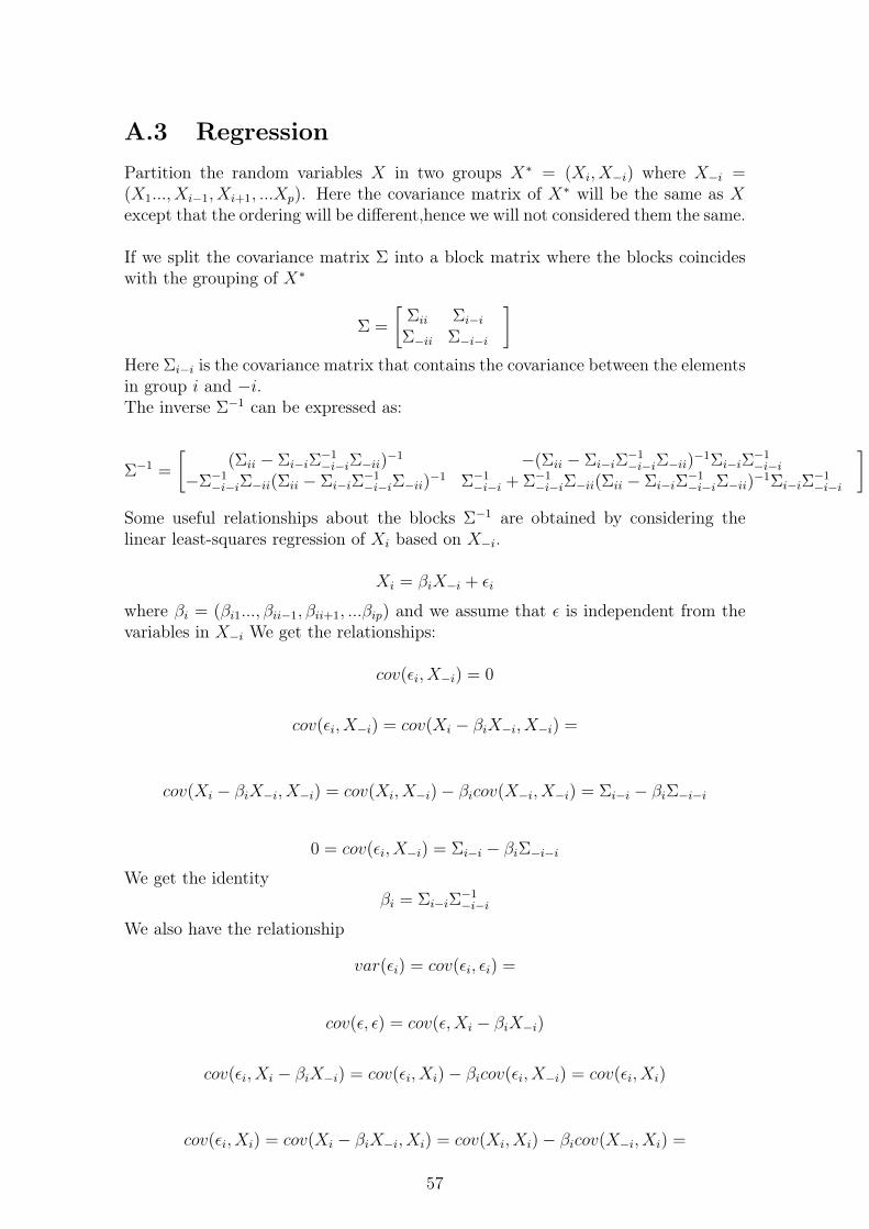
A.3 RegressionPartition the random variables X in two groups X∗ = (Xi, X−i) where X−i =(X1..., Xi−1, Xi+1, ...Xp). Here the covariance matrix of X∗ will be the same as Xexcept that the ordering will be different,hence we will not considered them the same.

If we split the covariance matrix Σ into a block matrix where the blocks coincideswith the grouping of X∗

Σ =

[Σii Σi−i

Σ−ii Σ−i−i

]Here Σi−i is the covariance matrix that contains the covariance between the elementsin group i and −i.The inverse Σ−1 can be expressed as:

Σ−1 =

[(Σii − Σi−iΣ

−1−i−iΣ−ii)

−1 −(Σii − Σi−iΣ−1−i−iΣ−ii)

−1Σi−iΣ−1−i−i

−Σ−1−i−iΣ−ii(Σii − Σi−iΣ

−1−i−iΣ−ii)

−1 Σ−1−i−i + Σ−1

−i−iΣ−ii(Σii − Σi−iΣ−1−i−iΣ−ii)

−1Σi−iΣ−1−i−i

]Some useful relationships about the blocks Σ−1 are obtained by considering thelinear least-squares regression of Xi based on X−i.

Xi = βiX−i + εi

where βi = (βi1..., βii−1, βii+1, ...βip) and we assume that ε is independent from thevariables in X−i We get the relationships:

cov(εi, X−i) = 0

cov(εi, X−i) = cov(Xi − βiX−i, X−i) =

cov(Xi − βiX−i, X−i) = cov(Xi, X−i)− βicov(X−i, X−i) = Σi−i − βiΣ−i−i

0 = cov(εi, X−i) = Σi−i − βiΣ−i−iWe get the identity

βi = Σi−iΣ−1−i−i

We also have the relationship

var(εi) = cov(εi, εi) =

cov(ε, ε) = cov(ε,Xi − βiX−i)

cov(εi, Xi − βiX−i) = cov(εi, Xi)− βicov(εi, X−i) = cov(εi, Xi)

cov(εi, Xi) = cov(Xi − βiX−i, Xi) = cov(Xi, Xi)− βicov(X−i, Xi) =

57

Σii − βiΣ−ii = Σii − Σi−iΣ−1−i−iΣ−ii

var(εi) = Σii − Σi−iΣ−1−i−iΣ−ii

var(εi) = Σii − βiΣ−iiWe see that row i can rewritten as

Σ−1 =

[(var(εi))

−1 −(var(εi))−1βi

∗ ∗

]It then follows that entries in Σ−1 has the regression-based interpretation:

Θii = (var(ε))−1

Θij = (var(ε))−1βij

This shows that the i,j entry of the precision matrix is, up to a scalar, the re-gression coefficient of variable j in the multiple regression of variable i on the rest[8].

An estimate of Θ can be obtained by regressingXi overX−i for i = 1, ..., p. Thereforewe can get an estimate Θ by estimating the β.

θii = ( ˆvar(εi))−1

θij = −( ˆvar(εi))−1βij

This means that the sparsity pattern in the partial correlations correspond to thesparsity pattern in the β.

A.4 SparsityTo constrain the log-likelihood (1), we add Lagrange constants for all missing edges

log(|Θ−1|) + trace(ΘS)−∑

(j,k)/∈E

γjkθjk (2)

The gradient equation for maximizing (2) can be written as

W − S − Γ = 0

Γ is a matrix of Lagrange parameters with nonzero values for all pairs with edgesabsent

If partition the variables in the matrices as in the regression (i,−i)[Wii Wi−iW−ii W−i−i

]−[Sii Si−iS−ii S−i−i

]−[

Γii Γi−iΓ−ii Γ−i−i

]= 0

And look at the lower left block, we have the equation

W−ii − S−ii − Γ−ii = 0

58

Since W = Θ−1 we have[Wii Wi−iW−ii W−i−i

] [Θii Θi−i

Θ−ii Θ−i−i

]=

[1 0

0T I

]

W−iiΘii +W−i−iΘ−ii = 0

W−ii = −W−i−iΘ−iiΘii

We remember from the regression identities that −Θ−iiΘii

= βTi

W−ii = W−i−iβTi

W−i−iβTi − S−ii − Γ−ii = 0

Now we can solve W−i−iβTi − S−ii − Γ−ii = 0 by simple subset regression. Supposethere are p − q nonzero elements in Γ−ii these correspond to the absent edges innode i. These p− q elements carry no information, therefore we can reduce βi to β∗iby removing its p− q elements corresponding to nonzero elements in Γ−ii. Yieldingthe reduced q × q system of equations.

W ∗−i−iβ

T∗i − S∗−ii = 0

Which we can solve for βT∗iβT∗i = W−1∗

−i−iS∗−ii

β∗i is padded with p− q zeros to give β. This leads to the simple iterative procedurefor each i.

W−ii = W−i−iβTi

Θ−ii = βTi Θii =βTi

Wii − βiW−ii

A.5 Graphical lassoThe gradient equation of (4) log(|Θ|)− trace(SΘ)− λ ‖Θ‖1 is

W − S − λSign(Θ)

where Sign(Θij) = sign(Θij) if Θij 6= 0 else Sign(Θij) ∈ [−1, 1]. If partition thevariables in the matrices as in the regression (i,−i)

[Wii Wi−iW−ii W−i−i

]−[Sii Si−iS−ii S−i−i

]− λ

[Sign(Θii) Sign(Θi−i)Sign(Θ−ii) Sign(Θ−i−i)

]= 0

And look at the lower left block, we have the equation

W−ii − S−ii − λSign(Θ−ii)

59

if we use that W−ii = −W−i−iΘ−iiΘii

and −Θ−iiΘii

= βTi we get

W−i−iβTi − S−ii − λSign(−βTi Θii)

W−i−iβTi − S−ii + λSign(βTi )

since Θii > 0. We will now see that this system is exactly equivalent to the estimatingequations for a lasso regression. Consider the lasso usual regression setup withoutcome variables y and predictor matrix Z.

1

2(y − Zβ)T (y − Zβ) + λ‖β‖1

The gradient expression is

ZTZβ − ZTy + λSign(β)

We see that if we define Z = W12−i−i and y = W

− 12

−i−iS−ii we get

W−i−iβTi − S−ii + λSign(βTi )

where β = βTi since we defined our regression as Xi = βiX−i + εi. This meansthat the solution of maximizing (4) is equivalent to a lasso regression problem, andtherefore called the graphical lasso.

60

Appendix B

R-code

B.1 Support functions

## func t i on s##l ibrary ( g l a s s o )l ibrary ( c l u s t e rGene ra t i on )l ibrary ( igraph )l ibrary (Matrix )l ibrary ( matr ixca l c )l ibrary ( tawny )

### Get p r i c e s ###

Get_p r i c e s = function ( ) {

Aurl = "http : //www. net fonds . no/quotes/kurs . php? exchange=OSE&s ec_types=&s e c t o r s=&t i c k s=&t ab l e=tab&s o r t=a lphabe t i c "

ak j s e r = read . csv ( Aurl , sep = "\ t " )

t i c k e r s = ak j s e r$paper

u = t i c k e r s [ 1 ]url = paste0 ( "http : //www. net fonds . no/quotes/paperh i s to ry . php?paper=" ,u ,

" .OSE&csv_format=txt " )S = as . data . frame ( read . table ( url ) )S$Date = as . Date (rownames(S) , format="%Y%m%d" )p r i c e s = S [ , c ( "Date" , " c l o s e " ) ]

colnames ( p r i c e s ) = c ( "Date" , t oS t r i ng (u) )

for ( t in 2 : length ( t i c k e r s ) ) {u = t i c k e r s [ t ]url = paste0 ( "http : //www. net fonds . no/quotes/paperh i s to ry . php?paper=" ,

u , " .OSE&csv_format=txt " )

S = as . data . frame ( read . table (url , header = TRUE) )

S$Date = as . Date (rownames(S) , format="%Y%m%d" )

61

tmp = S [ , c ( "Date" , " c l o s e " ) ]

colnames (tmp) = c ( "Date" , t oS t r i ng (u) )

i f (nrow(S) > 0) {p r i c e s = merge( p r i c e s , tmp ,by = "Date" , a l l = TRUE)

}

}

return ( p r i c e s )

}

#pr i c e s = Get_p r i c e s ( )

###Get obx index

Get_OBX = function ( ) {

u = "OBX"url = paste0 ( "http : //www. net fonds . no/quotes/paperh i s to ry . php?paper=" ,u ,

" .OSE&csv_format=txt " )S = as . data . frame ( read . table ( url ) )S$Date = as . Date (rownames(S) , format="%Y%m%d" )obx = S [ , c ( "Date" , " c l o s e " ) ]

row .names( obx ) = obx$Dateobx = obx [ order ( obx$Date ) , ]

return ( obx )}

##Get count o f s t o c k s t ha t as na% over a c u t o f f ###

Get_NA = function ( p r i c e s ,Window , c u t o f f ) {

nonNA = data . frame ( )

for ( i in 1 : (nrow( p r i c e s )−Window) ) {

p r i c e s_set = pr i c e s [(1+ i ) : (Window+i ) , ]

na_count <−( sapply ( p r i c e s_set , function ( y ) sum( length (which( i s .na( y ) )) )/nrow( p r i c e s_set ) ) )

nonNA = rbind (nonNA, c ( i , length (which(na_count<cu t o f f ) ) ) )

62

#i f ( l e n g t h ( which (na_count <0.1) ) == 0) break

}

return (nonNA)

}

f i l lNA = function (X) {

X[which( i s .na(X) ) ] = mean(X,na .rm = T)return (X)

}

#ca l c u l a t e Logreturns form pr i c e s

makereturns = function (P,LOG = TRUE){

end = nrow(P)

Returns = P

for ( i in 1 : ncol (P) ) {a = (P[ , i ] / c (NA, P[ , i ] [ 1 : ( end−1) ] ) ) − 1i f (LOG == TRUE) {a = log ( a+1)} #turn o f f i f a r i t hme t i c }

Returns [ , i ] = a

}

return ( Returns [ −1 , ] )

}

###opt imal Weights f o r GMVP

FindWeights = function (INV) {ones = rep (1 ,nrow(INV) )W = (INV%∗%t ( t ( ones ) ) ) / ( ones%∗%INV%∗%t ( t ( ones ) ) ) [ [ 1 ] ]return (W)

}

63

##AIC BIC EBIC

IC = function (Te) {

ML = log ( det (Te) )−sum(diag (Te%∗%SCOV) )

d = sum(Te [upper . t r i (Te) ] != 0)

pa = 1

return (c(−N∗ML+2∗d,−N∗ML+d∗log (N) ,−N∗ML+d∗log (N)+4∗d∗pa∗log (P) ) )

}

##STARS

STARS = function (Nn=20,b= min(round( sqrt (N)∗10) , 0 . 7∗N) , lam) {Tet = matrix (0 ,P,P)for ( s in 1 :Nn) {

SIM_i = SIM [ sample ( seq ( 1 :N) ,b) , ]

i f ( lam !=0 ) {gl_i = g l a s s o (cov (SIM_i ) , lam )$wi

}

i f ( lam ==0 ) {gl_i = solve (cov (SIM_i ) )

}

gl_i [which( gl_i !=0) ] = 1Tet = Tet+gl_i#pr in t ( s )

}Tet = Tet/NnEp = 2∗Tet∗(1−Tet )D = sum(Ep [upper . t r i (Ep) ] ) /choose (P, 2 )return (D)

}

###CV

CrossVal id = function (SIM , k = 5 , lam ) {old <− .Random . seedon . exit ( { .Random . seed <<− old } )set . seed (1 )

f o l d s = rep ( 1 : k , each= N/k )

i f ( (N−length ( f o l d s ) ) != 0) {

64

f o l d s = c ( f o l d s , sample ( seq ( 1 : k ) , (N−length ( f o l d s ) ) , replace = T) )

}

f o l d s = f o l d s [ sample ( seq ( 1 :N) ,N) ]CV = c ( 0 , 0 )

for (cvK in 1 : k ) {

inF = SIM [which( f o l d s ==cvK) , ]outF = SIM [which( f o l d s !=cvK) , ]

covIN = cov ( inF )i f ( lam !=0 ) {

glssoOUT = g l a s s o (cov ( outF ) , lam )$wi#glassoIN = g l a s s o ( covIN , lam)$wi

}

i f ( lam ==0 ) {glssoOUT = solve (cov ( outF ) )#glassoIN = so l v e ( covIN )

}W_out = FindWeights ( glssoOUT)var_in = var ( inF%∗%W_out )

CV_k_1 = −log ( det ( glssoOUT) )+sum(diag ( glssoOUT%∗%covIN ) )CV_k_2 = var_in #log ( de t ( g lassoIN ) )−sum( diag ( g lassoIN%∗%cov ( outF ) ) )

CV = CV+c (CV_k_1 ,CV_k_2)

}

return (CV)

}

Pre fCrossVal id = function ( k = 5 , lam ) {old <− .Random . seedon . exit ( { .Random . seed <<− old } )set . seed (1 )

f o l d s = rep ( 1 : k , each= N/k )

i f ( (N−length ( f o l d s ) ) != 0) {

f o l d s = c ( f o l d s , sample ( seq ( 1 : k ) , (N−length ( f o l d s ) ) , replace = T) )

}

f o l d s = f o l d s [ sample ( seq ( 1 :N) ,N) ]CV = 0

for (cvK in 1 : k ) {

inF = SIM [which( f o l d s ==cvK) , ]

65

outF = SIM [which( f o l d s !=cvK) , ]

covIN = cov ( inF )i f ( lam !=0 ) {

glssoOUT = g l a s s o (cov ( outF ) , lam )$wi}

i f ( lam ==0 ) {glssoOUT = solve (cov ( outF ) )

}

W_out = FindWeights ( glssoOUT)var_in = var ( inF%∗%W_out )

CV = CV+var_in

}

return (CV)

}

##Generate comunity matrix

SBGG =function ( Nclust , inP , outP ) {

Cmat = matrix (0 ,P,P)c l u s t e r s = sample ( 1 : Nclust ,P, replace =T)

for ( i in 1 : Nclust ) {Cmat [which( c l u s t e r s == i ) ,which( c l u s t e r s == i ) ] = 1

}

i n c l u s t = which(Cmat [upper . t r i (Cmat) ]==1)ou t c l u s t = which(Cmat [upper . t r i (Cmat) ]==0)

Cmat [upper . t r i (Cmat) ] [ ou t c l u s t ] = rbinom( length ( ou t c l u s t ) ,1 , outP )Cmat [upper . t r i (Cmat) ] [ i n c l u s t ] = rbinom( length ( i n c l u s t ) ,1 , inP )

diag (Cmat) = 1

Cmat [ lower . t r i (Cmat) ] = t (Cmat) [ lower . t r i (Cmat) ]

graphobj = graph_from_adjacency_matrix (Cmat−diag (P) )V( graphobj )$ c o l o r = sample ( colors ( ) , Nclust ) [ c l u s t e r s ]

66

SBG = l i s t ( )SBG$MAT = CmatSBG$G = graphobjSBG$Clust = c l u s t e r s

return (SBG)

}

Gen_dataFromSparse = function (L ,MV, Ki = 0 . 1 ) {

L = L+ diag ( rep (abs (min( eigen (L)$va lue s ) ) +0.001 ,P) )#as . matrix (nearPD(L, corr = TRUE, maxit = 1000)$mat)

#COR = cov2cor ( genPosi t iveDefMat (dim = P)$Sigma )

K = P∗Ki

W = matrix (rnorm(P∗K,mean=0,sd=1) , P, K)S = W%∗%t (W) + diag ( runif (P) )COR = diag (1/sqrt (diag (S) ) )%∗%S%∗%diag (1/sqrt (diag (S) ) )

ru = runif (P, min = 0.0001 , max = (1/MV)^2)COV = diag ( sqrt ( ru ) )%∗%COR%∗%diag ( sqrt ( ru ) )ICOV = solve (COV)

e i g v a l s = runif (P, min = 0.0001 , max = (1/MV)^2∗min(diag (L) ) )

V = eigen (COV)$vector

newCOV = V%∗%diag ( ( sort ( e i g v a l s ) ) )%∗%t (V)newICOV = solve (newCOV)

spICOV = newICOV∗L

SpCOV = solve (spICOV)

SIM = mvrnorm(N, rep (0 ,P) ,SpCOV)

SPret = l i s t ( )

SPret$INV = spICOVSPret$COV = SpCOVSPret$SIM = SIM

return ( SPret )}

B.2 Predicting power vs graph recovery

67

NN = rev ( seq (40 ,100 ,10) )

KL_NN_S = data . frame ( )F1_NN_S = data . frame ( )

for ( s i in 1 : 100 ) {

P = 50

G_S = SBGG(round( log (P) ) , 1 , 0 . 0 1 )

#p l o t ( G_S$G, ve r t e x . s i z e =2, v e r t e x . l a b e l=NA, edge . arrow . s i z e =0)

Cmat = G_S$MAT

KL_NN = rep (0 , length (NN) )F1_NN = rep (0 , length (NN) )

for (N in NN){

SPsim = Gen_dataFromSparse (L = Cmat ,MV = 25)

spICOV = SPsim$INVSpCOV = SPsim$COV

SIM = SPsim$SIM

SCOV = cov (SIM)

max_lambda = max(abs (SCOV[upper . t r i (SCOV) ] ) )min_lambda = max_lambda∗0 .01#min( abs (SCOV[ upper . t r i (SCOV) ] ) )

#lambda_range = seq (min_lambda ,max_lambda , l e n g t h . out = 50)

lambda_range = quantile (abs (SCOV[upper . t r i (SCOV) ] ) , seq (0 , 1 , length .out = 50) ) [−1]

KL = rep (0 , length ( lambda_range ) )F1 = rep (0 , length ( lambda_range ) )

68

for ( i in 1 : length ( lambda_range ) ) {

GraphLasso = g l a s s o (SCOV, lambda_range [ i ] ) $wi

G_structure = GraphLassoG_structure [which(G_structure != 0) ] = 1

TN = sum(G_structure+Cmat == 0)TP = sum(G_structure+Cmat == 2)

AllP = sum(Cmat == 1)AllN = sum(Cmat == 0)

FP = AllN−TNFN = AllP−TP

sens = TP/ (TP+FN)spec = TN/ (TN+FP)

MCC = (TP∗TN−FP∗FN)/ ( sqrt (TP + FP)∗sqrt (TP + FN)∗sqrt (TN + FP)∗sqrt (TN + FN) )

F1 [ i ] = 2∗TP/(2∗TP+FN+FP)

KL[ i ] = (sum(diag (SpCOV%∗%GraphLasso ) )−log ( det (SpCOV%∗%GraphLasso ) )−P)/2

}

W_KL = lambda_range [which .min(KL) ]W_F1 = lambda_range [which .max(F1) ]

F1_NN[ (which(N ==NN) ) ] = sum( ( FindWeights (spICOV)−FindWeights (g l a s s o (SCOV,W_F1)$wi ) ) ^2)

KL_NN[ (which(N ==NN) ) ] = sum( ( FindWeights (spICOV)−FindWeights (g l a s s o (SCOV,W_KL)$wi ) ) ^2)

print (N)}

F1_NN_S = rbind (F1_NN_S , F1_NN)KL_NN_S = rbind (KL_NN_S ,KL_NN)

print ( s i )

}

69

F1_AVG = apply (F1_NN_S , 2 ,mean)KL_AVG = apply (KL_NN_S , 2 ,mean)

B.3 Best tuning parameter method

NN = rev ( seq (40 ,100 ,10) )

AIC_NN_S = data . frame ( )BIC_NN_S = data . frame ( )EBIC_NN_S = data . frame ( )Star_NN_S = data . frame ( )CV_NN_S = data . frame ( )CV_P_NN_S = data . frame ( )Or_NN_S = data . frame ( )

for ( s i in 1 : 10 ) {

P = 50


#p l o t ( G_S$G, ve r t e x . s i z e =2, v e r t e x . l a b e l=NA, edge . arrow . s i z e =0)

Cmat = G_S$MAT

AIC_NN = rep (0 , length (NN) )BIC_NN = rep (0 , length (NN) )EBIC_NN = rep (0 , length (NN) )Star_NN = rep (0 , length (NN) )CV_NN = rep (0 , length (NN) )CV_P_NN = rep (0 , length (NN) )Or_NN = rep (0 , length (NN) )

for (N in NN){

SPsim = Gen_dataFromSparse (L = Cmat ,MV = 25 ,Ki=0.1)

spICOV = SPsim$INVSpCOV = SPsim$COV

70

SIM = SPsim$SIM

SCOV = cov (SIM)


AIC = rep (0 , length ( lambda_range ) )BIC = rep (0 , length ( lambda_range ) )EBIC = rep (0 , length ( lambda_range ) )Star = rep (0 , length ( lambda_range ) )CV = rep (0 , length ( lambda_range ) )CV_P = rep (0 , length ( lambda_range ) )

WeD = rep (0 , length ( lambda_range ) )

for ( i in 1 : length ( lambda_range ) ) {

GraphLasso = g l a s s o (SCOV, lambda_range [ i ] ) $wi

G_structure = GraphLassoG_structure [which(G_structure != 0) ] = 1

WeD[ i ] = sum( ( FindWeights (spICOV)−FindWeights (GraphLasso ) ) ^2)

AIC [ i ] = IC(GraphLasso ) [ 1 ]BIC [ i ] = IC(GraphLasso ) [ 2 ]EBIC [ i ] = IC(GraphLasso ) [ 3 ]Star [ i ] = STARS( lam = lambda_range [ i ] )

CV_M = CrossVal id (SIM , lam = lambda_range [ i ] )CV[ i ] = CV_M[ 1 ]CV_P[ i ] = CV_M[ 2 ]

}

W_AIC = lambda_range [which .min(AIC) ]W_BIC = lambda_range [which .min(BIC) ]W_EBIC = lambda_range [which .min(EBIC) ]

starC = which( Star <0.05)i f ( length ( starC )>1){W_Star = lambda_range [which( Star <0.05) [ 2 ] ]

}

i f ( length ( starC )==1){

71

W_Star = lambda_range [ starC ]}

W_CV = lambda_range [which .min(CV) ]W_CVP = lambda_range [which .min(CV_P) ]

W_o r a c l e = lambda_range [which .min(WeD) ]

AIC_NN[ (which(N ==NN) ) ] = sum( ( FindWeights (spICOV)−FindWeights (g l a s s o (SCOV,W_AIC)$wi ) ) ^2)

print (AIC_NN[ (which(N ==NN) ) ] )

BIC_NN[ (which(N ==NN) ) ] = sum( ( FindWeights (spICOV)−FindWeights (g l a s s o (SCOV,W_BIC)$wi ) ) ^2)

EBIC_NN[ (which(N ==NN) ) ] = sum( ( FindWeights (spICOV)−FindWeights (g l a s s o (SCOV,W_EBIC)$wi ) ) ^2)

Star_NN[ (which(N ==NN) ) ] = sum( ( FindWeights (spICOV)−FindWeights (g l a s s o (SCOV,W_Star )$wi ) ) ^2)

CV_NN[ (which(N ==NN) ) ] = sum( ( FindWeights (spICOV)−FindWeights (g l a s s o (SCOV,W_CV)$wi ) ) ^2)

CV_P_NN[ (which(N ==NN) ) ] = sum( ( FindWeights (spICOV)−FindWeights (g l a s s o (SCOV,W_CVP)$wi ) ) ^2)

Or_NN[ (which(N ==NN) ) ] = sum( ( FindWeights (spICOV)−FindWeights (g l a s s o (SCOV,W_o r a c l e )$wi ) ) ^2)

print (N)}

AIC_NN_S = rbind (AIC_NN_S ,AIC_NN)BIC_NN_S = rbind (BIC_NN_S ,BIC_NN)EBIC_NN_S = rbind (EBIC_NN_S ,EBIC_NN)Star_NN_S = rbind ( Star_NN_S , Star_NN)CV_NN_S = rbind (CV_NN_S ,CV_NN)CV_P_NN_S = rbind (CV_P_NN_S ,CV_P_NN)Or_NN_S = rbind (Or_NN_S ,Or_NN)print ( s i )

}

AIC_AVG = apply (AIC_NN_S , 2 ,mean)BIC_AVG = apply (BIC_NN_S , 2 ,mean)EBIC_AVG = apply (EBIC_NN_S , 2 ,mean)Star_AVG = apply ( Star_NN_S , 2 ,mean)CV_AVG = apply (CV_NN_S , 2 ,mean)CV_P_AVG = apply (CV_P_NN_S , 2 ,mean)Or_AVG = apply (Or_NN_S , 2 ,mean)

B.4 Simulated data

ind = 100

P = 50

72

ANW = data . frame ( )ANGW1 = data . frame ( )ANEW = data . frame ( )ANTW = data . frame ( )

NW = rep ( 0 , 7 )NGW1 = rep ( 0 , 7 )NEW = rep ( 0 , 7 )NTW = rep ( 0 , 7 )

for (N in rev ( seq (40 ,100 ,10) ) ) {

timeW = array (0 ,dim=c (P, 1 , ind ) )timeGW1 = array (0 ,dim=c (P, 1 , ind ) )timeEW = array (0 ,dim=c (P, 1 , ind ) )timeTW = array (0 ,dim=c (P, 1 , ind ) )

for ( i in 1 : ind ) {


plot ( G_S$G, ver tex . s i z e =2, ver tex . l a b e l=NA, edge . arrow . s i z e =0)

Cmat = G_S$MAT


ICOV = SPsim$INVCOV = SPsim$COV

SIM = SPsim$SIM

Pret = SIM

SCOV = cov ( Pret )

i f (P<N){ISCOV = solve (SCOV)

}

i f (P>=N){ISCOV = ginv (SCOV)

73

}


CV1 = rep (0 , length ( lambda_range ) )

for ( l a in 1 : length ( lambda_range ) ) {

CV_M = CrossVal id (SIM , lam = lambda_range [ l a ] )CV1[ l a ] = CV_M[ 1 ]

}

GL1 = g l a s s o (SCOV, lambda_range [which .min(CV1) ] )GLl1 = GL1$wi

P_W = FindWeights (ISCOV)P_GW1 = FindWeights (GLl1 )P_EW = rep (1/P,P)P_TW = FindWeights (ICOV)

timeW [ , , i ] = P_WtimeGW1 [ , , i ] = P_GW1timeEW[ , , i ] = P_EWtimeTW[ , , i ] = P_TW

print ( i )}

W = 0GW1 = 0EW = 0

for ( i i in 1 : ind ) {

W = W +sum(abs (timeW [ , , i i ]−timeTW[ , , i i ] ) )GW = GW + sum(abs (timeGW[ , , i i ]−timeTW[ , , i i ] ) )GW1 = GW1 + sum(abs (timeGW1 [ , , i i ]−timeTW[ , , i i ] ) )EW = EW + sum(abs (timeEW[ , , i i ]−timeTW[ , , i i ] ) )}

W = W/ indGW = GW/ indGW1 = GW1/ indEW = EW/ ind

NW[which(N == rev ( seq (40 ,100 ,10) ) ) ] = W

74

NGW[which(N == rev ( seq (40 ,100 ,10) ) ) ] = GWNGW1[which(N == rev ( seq (40 ,100 ,10) ) ) ] = GW1NEW[which(N == rev ( seq (40 ,100 ,10) ) ) ] = EW

}###OUT−OF−SAMPLE##

ind = 100

P = 50

ANW = data . frame ( )ANGW = data . frame ( )ANGW1 = data . frame ( )ANEW = data . frame ( )ANTW = data . frame ( )

NW = rep ( 0 , 7 )NGW = rep ( 0 , 7 )NGW1 = rep ( 0 , 7 )NEW = rep ( 0 , 7 )NTW = rep ( 0 , 7 )

for (N in rev ( seq (40 ,100 ,10) ) ) {

timeW = array (0 ,dim=c (1 , 1 , ind ) )timeGW = array (0 ,dim=c (1 , 1 , ind ) )timeGW1 = array (0 ,dim=c (1 , 1 , ind ) )timeEW = array (0 ,dim=c (1 , 1 , ind ) )timeTW = array (0 ,dim=c (1 , 1 , ind ) )

for ( i in 1 : ind ) {


plot ( G_S$G, ver tex . s i z e =2, ver tex . l a b e l=NA, edge . arrow . s i z e =0)

Cmat = G_S$MAT


ICOV = SPsim$INVCOV = SPsim$COV

SIM1 = mvrnorm(N, rep (0 ,P) ,COV)SIM2 = mvrnorm(N, rep (0 ,P) ,COV)Pret = SIM1

75

SCOV = cov ( Pret )

i f (P<N){ISCOV = solve (SCOV)

}

i f (P>=N){ISCOV = ginv (SCOV)

}

lambda_range = quantile (abs (SCOV[upper . t r i (SCOV) ] ) , seq (0 , 1 , length. out = 50) ) [−1]

CV1 = rep (0 , length ( lambda_range ) )


CV_M = CrossVal id (SIM1 , lam = lambda_range [ l a ] )CV1[ l a ] = CV_M[ 1 ]

}

GL1 = g l a s s o (SCOV, lambda_range [which .min(CV1) ] )GLl1 = GL1$wi

P_W = FindWeights (ISCOV)P_GW1 = FindWeights (GLl1 )P_EW = rep (1/P,P)P_TW = FindWeights (ICOV)

R_W = SIM2%∗%P_WR_GW1 = SIM2%∗%P_GW1R_EW = SIM2%∗%P_EWR_TW = SIM2%∗%P_TW

timeW [ , , i ] = var (R_W)timeGW1 [ , , i ] = var (R_GW1)timeEW[ , , i ] = var (R_EW)timeTW[ , , i ] = var (R_TW)

print ( i )}

W = 0GW = 0GW1 = 0EW = 0TW = 0

76

for ( i i in 1 : ind ) {

W = W +timeW [ , , i i ]GW1 = GW1 + timeGW1 [ , , i i ]EW = EW + timeEW[ , , i i ]TW = TW + timeTW[ , , i i ]

}

W = W/ indGW1 = GW1/ indEW = EW/ indTW = TW/ ind

NW[which(N == rev ( seq (40 ,100 ,10) ) ) ] = WNGW1[which(N == rev ( seq (40 ,100 ,10) ) ) ] = GW1NEW[which(N == rev ( seq (40 ,100 ,10) ) ) ] = EWNTW[which(N == rev ( seq (40 ,100 ,10) ) ) ] = TW

}

B.5 Real data

p r i c e s = Get_p r i c e s ( )

row .names( p r i c e s ) = p r i c e s$Datep r i c e s = p r i c e s [ ,−1]

NAS = Get_NA( pr i c e s , 1 0 0 , 0 . 0 5 )

cutp = which(NAS[ ,2] >=90) [ 1 ]

Pr i ce = p r i c e s [ cutp :nrow( p r i c e s ) , ]

Pret = makereturns ( Pr i ce )

PretCUT = Pret

ind = c (0 , seq ( 1 : (nrow(PretCUT)−100) ) )

timeW = array (0 ,dim=c (ncol (PretCUT) ,1 , length ( ind ) ) )timeGW = array (0 ,dim=c (ncol (PretCUT) ,1 , length ( ind ) ) )timeLW = array (0 ,dim=c (ncol (PretCUT) ,1 , length ( ind ) ) )timeEW = array (0 ,dim=c (ncol (PretCUT) ,1 , length ( ind ) ) )lambdas = rep (0 , length ( ind ) )

for ( i in ind ) {

r e t_sub = PretCUT[(1+ i ) :(100+ i ) , ]

77

na_count <−( sapply ( r e t_sub , function ( y ) sum( length (which( i s .na( y ) ) ) )/nrow( r e t_sub ) ) )

r e t_sub = re t_sub [ ,which(na_count<=0.1) ]r e t_sub = sapply ( r e t_sub , function ( y ) f i l lNA (y ) )

N =dim( r e t_sub ) [ 1 ]P = dim( r e t_sub ) [ 2 ]

i f (P<N){ISCOV = solve (SCOV)}

i f (P>=N){ISCOV = ginv (SCOV)}

Pmat =matrix (0 ,P,P)

for ( gg in 1 : length ( grouping ) ) {Pmat [which( grouping == gg ) ,which( grouping == gg ) ] = 1}

diag (Pmat) = 1

Pmat = 1−PmatPmat [which(Pmat ==0) ] = 0 .5

max_lambda = max(abs (SCOV[upper . t r i (SCOV) ] ) )min_lambda = max_lambda∗0 .01#min( abs (SCOV[ upper . t r i (SCOV) ] ) ) #max_

lambda∗0.01lambda_range = quantile (abs (SCOV[upper . t r i (SCOV) ] ) , seq (0 , 1 , length . out

= 50) ) [−1]

lambda_range = seq (min_lambda ,max_lambda , length . out = 50)

CV = rep (0 , length ( lambda_range ) )


GraphLasso = g l a s s o (SCOV, lambda_range [ l a ] ) $wi

CV_M = CrossVal id (SIM = re t_sub , lam = lambda_range [ l a ] )

CV[ l a ] =CV_M[ 1 ]}

LW_SCOV = cov_shr ink ( r e t_sub )LW_ISCOV = solve (SCOV)lambdas [ ind+1] = which .min(CV)

GL = g l a s s o (SCOV, lambda_range [which .min(CV) ] )GL = g l a s s o (SCOV, lambda_range [ 1 ] )

78

GLl = GL$wi

P_W = FindWeights (ISCOV)P_GW = FindWeights (GLl )P_EW = FindWeights (diag (P) )P_LW = FindWeights (LW_ISCOV)

timeW [ , , i +1] [match(colnames ( r e t_sub ) ,colnames ( Pret ) ) ] = P_WtimeGW[ , , i +1] [match(colnames ( r e t_sub ) ,colnames ( Pret ) ) ] = P_GWtimeEW[ , , i +1] [match(colnames ( r e t_sub ) ,colnames ( Pret ) ) ] = P_EWtimeLW[ , , i +1] [match(colnames ( r e t_sub ) ,colnames ( Pret ) ) ] = P_EW

print ( i )}

port_r e t = rep ( 0 , (nrow(PretCUT)−100) )portE_r e t = rep ( 0 , (nrow(PretCUT)−100) )portG_r e t = rep ( 0 , (nrow(PretCUT)−100) )portLW_r e t = rep ( 0 , (nrow(PretCUT)−100) )

for ( i in 1 : (nrow(PretCUT)−100) ) {

port_r e t [ i ] = (sum(PretCUT[(100+ i ) , ] ∗timeW [ , , i ] ,na .rm = T) )portE_r e t [ i ] = (sum(PretCUT[(100+ i ) , ] ∗timeEW[ , , i ] ,na .rm = T) )portG_r e t [ i ] = (sum(PretCUT[(100+ i ) , ] ∗timeGW[ , , i ] ,na .rm = T) )portLW_r e t [ i ] = (sum(PretCUT[(100+ i ) , ] ∗timeLW [ , , i ] ,na .rm = T) )

}

79

shatthik barua master’s thesis, spring 2017

Documents