Joint Defra/EA Flood and Coastal Erosion Risk Management R&D Programme

Shell Hybrid Model Interface Manual R&D Technical Report FD2107/TR Produced: December 2007 Author(s):

1

Statement of use Dissemination status Keywords: Research contractor: Defra project officer: Publishing organisation Department for Environment, Food and Rural Affairs Flood Management Division, Ergon House, Horseferry Road London SW1P 2AL

Tel: 020 7238 3000 Fax: 020 7238 6187

www.defra.gov.uk/environ/fcd

© Crown copyright (Defra);(insert year) Copyright in the typographical arrangement and design rests with the Crown. This publication (excluding the logo) may be reproduced free of charge in any format or medium provided that it is reproduced accurately and not used in a misleading context. The material must be acknowledged as Crown copyright with the title and source of the publication specified. The views expressed in this document are not necessarily those of Defra or the Environment Agency. Its officers, servants or agents accept no liability whatsoever for any loss or damage arising from the interpretation or use of the information, or reliance on views contained herein. Published by the Department for Environment, Food and Rural Affairs (insert month, year). Printed on material that contains a minimum of 100% recycled fibre for uncoated paper and 75% recycled fibre for coated paper. PB No. xxxxx

2

Acknowledgements This project FD2107 addressed mainly (iii), developing Hybrid models for (50-year) morphological prediction (combining advantages of T-D and B-U approaches). Several models were applied for different intervention and climate change scenarios to identify the impacts on the levels and form of eight varied UK estuaries. This work was funded by the Environment Agency and Department for Environment, Food and Rural Affairs (Defra), whose support is gratefully acknowledged. Software support and/or comments have been provided by the following organisations: Wallingford Software; Danish Hydraulic Institute; and HR Wallingford.

i

Contents Page

Acknowledgements.................................................................................................................. i Contents.................................................................................................................................. ii Part 1. Introduction ................................................................................................................. 1

1.1 About This Manual .......................................................................................... 1 1.2 What is the HMI?............................................................................................. 1 1.3 What is Regime Theory?................................................................................. 2 1.4 Product Overview ............................................................................................ 4 1.5 What the HMI Interface Cannot Do! ................................................................ 5

1.5.1 Waves.................................................................................................. 5 1.5.2 Sediment.............................................................................................. 5 1.5.3 Bed Updating....................................................................................... 6

1.6 System Requirements ..................................................................................... 6 1.7 Installing the Hybrid Model Interface ............................................................... 7

Part 2. Using the Hybrid Model Interface................................................................................ 9 2.1 Step One ......................................................................................................... 9

2.1.1 Applies To All Models .......................................................................... 9 2.2 Getting Started ................................................................................................ 9

2.2.1 Applies to All Models ........................................................................... 9 2.2.2 Mike11 Users Only ............................................................................ 10

2.3 Model Simulation - Initial Setup Conditions................................................... 11 2.3.1 Applies To All Models ........................................................................ 11 2.3.2 Assumptions ...................................................................................... 11

2.4 Model Boundary - Initial Setup Conditions .................................................... 12 2.4.1 Applies To All Models ........................................................................ 12 2.4.2 Flood or Ebb Dominance................................................................... 13

2.5 Network Setup - Initial Setup Conditions ....................................................... 14 2.5.1 Applies To All Models ........................................................................ 14

2.6 Cross-Section File - Initial Setup Conditions ................................................. 16 2.6.1 Applies To All Models ........................................................................ 16

2.7 Output Settings.............................................................................................. 19 2.7.1 Mike11 Users Only ............................................................................ 19

2.8 Hydrodynamic File - Initial Setup Conditions................................................. 20 2.8.1 Mike11 Users Only ............................................................................ 20

2.9 Hydrodynamic File – Output Time-Step ........................................................ 21 2.10 Connecting to the Model ............................................................................... 21

2.10.1 Mike11 Users Only ............................................................................ 21 2.10.2 InfoWorks Users Only........................................................................ 22 2.10.3 InfoWorks Folder and File Structure .................................................. 23 2.10.4 Save and Load InfoWorks Setup Information .................................... 23 2.10.5 Initialise the Model ............................................................................. 24

2.11 Changing the Bathymetry.............................................................................. 25 2.11.1 Applies to all models.......................................................................... 25 2.11.2 Editing a Single Point......................................................................... 26 2.11.3 Editing Multiple Points ....................................................................... 26 2.11.4 Mike11 Users Only ............................................................................ 27 2.11.5 InfoWorks Users Only........................................................................ 28

2.12 Reading the Hydrodynamic Data................................................................... 28 2.12.1 Applies to all Models.......................................................................... 28 2.12.2 Parameter Base................................................................................. 29 2.12.3 Regime Forcing ................................................................................. 29 2.12.4 Exclude Selected Cross-Sections...................................................... 31

ii

2.12.5 Regime Type ..................................................................................... 32 2.13 Existing Data Information .............................................................................. 33 2.14 Analysing the Hydrodynamic Data ................................................................ 34

2.14.1 Mike11 Users Only ............................................................................ 34 2.14.2 InfoWorks Users Only........................................................................ 35

2.15 Regime Menu Options................................................................................... 35 2.15.1 Applies To All Models ........................................................................ 35

2.16 Defining the Regime Options......................................................................... 44 2.16.1 Applies to all Users ............................................................................ 44 2.16.2 Mike11 Users Only ............................................................................ 51 2.16.3 InfoWorks Users Only........................................................................ 53

2.17 Running a Regime Simulation....................................................................... 54 2.17.1 Applies to all Users ............................................................................ 54

2.18 Model Calibration and Validation................................................................... 57 2.18.1 Applies to all Users ............................................................................ 57

Part 3. Technical Information................................................................................................ 59 3.1 Tidal Asymmetry............................................................................................ 59

3.1.1 Dronkers Tidal Asymmetry Ratio ....................................................... 60 3.1.2 Slack Gradient ................................................................................... 60 3.1.3 Slack Duration ................................................................................... 61 3.1.4 Tidal Excursion .................................................................................. 61

3.2 1D Energy Terms .......................................................................................... 61 3.3 Morphological Tide ........................................................................................ 63

3.3.1 Sediment Transport Relationships..................................................... 64 3.4 Bed Updating Routine ................................................................................... 66

3.4.1 Applies to all Users ............................................................................ 66 3.5 Proposed Approach....................................................................................... 70

3.5.1 Hypsometry Method........................................................................... 70 3.6 Constraint File ............................................................................................... 74

3.6.1 Applies to all Users ............................................................................ 74 3.7 Estimate of Estuary Water Volume................................................................ 76

3.7.1 Applies to all Users ............................................................................ 76 3.8 Boundary Conditions – Sea level Rise Scenario ........................................... 77

3.8.1 Applies to all Users ............................................................................ 77 3.9 Mike11 - Res11Read.exe file ........................................................................ 78

3.9.1 Mike11 Users Only ............................................................................ 78 3.10 Mike11 – Xfs Tool.......................................................................................... 78

3.10.1 Mike11 Users Only ............................................................................ 78 3.11 InfoWorks RS.com Tools............................................................................... 79

3.11.1 InfoWorks Users Only........................................................................ 79 3.12 Shell Interface Code...................................................................................... 79

Part 4. Trouble Shooting....................................................................................................... 82 4.1 Cannot Locate The Mike11 Executable File.................................................. 82 4.2 Not Able to Read the Mike11 Simulation File ................................................ 82 4.3 Known Problems ........................................................................................... 84

3.12.1 Mike11 User Only .............................................................................. 84 Part 5. References................................................................................................................ 86 Figures 1. An idealised view of how the HMI works..................................................................... 2 2. Changes in flow speed across a transverse profile..................................................... 6 3. Initial setup screen ...................................................................................................... 7

iii

4. Matlab setup and installation program ........................................................................ 8 5. Selecting the HMI termed ‘Shell Interface’ .................................................................. 9 6. The initial screen displayed in the HMI ..................................................................... 10 7. Directory mapping location for Mike11.exe file ......................................................... 10 8. The read baseline hydrodynamic control form .......................................................... 13 9. Position of peak discharge for a baseline and scenario condition............................. 14 10. Water level and corresponding discharge value for a selected cross-section........... 14 11. HR Wallingford ISIS model of Tollesbury Creek ....................................................... 15 12. Cross-sections (black lines) defined within Southampton Water .............................. 16 13. Amended section profile............................................................................................ 17 14. Resolved cross-section profile .................................................................................. 18 15. An example of a cross-section profile with a high degree of bathymetry

scatter along the intertidal margins ........................................................................... 19 16. Save results from the cross-section positions only ................................................... 20 17. Correctly ordering the output from the Mike11 model ............................................... 20 18. Required additional items in Mike11 ......................................................................... 21 19. Baseline Mike11 simulation form .............................................................................. 22 20. Baseline InfoWorks simulation form.......................................................................... 23 21. Using the Load and Save functions to store and retrieve the simulation setup

parameters ................................................................................................................ 24 22. Baseline InfoWorks simulation form.......................................................................... 24 23. Simulation file form.................................................................................................... 25 24. Matlab generated GUI............................................................................................... 26 25. Matlab cross-section editor GUI................................................................................ 27 26. Regime coefficients displayed on the control form.................................................... 28 27. Regime fit (Cross-section area vs Maximum discharge).......................................... 30 28. Select excluded cross-section................................................................................... 31 29. Example of file format needed to exclude cross-section........................................... 32 30. Dialog box asking the user if the information contained within the specified

folder structure can be deleted.................................................................................. 33 31. View asking Mike11 users to select the additional result file..................................... 34 32. Read existing hydrodynamic information form .......................................................... 35 33. Parametric plots for the selected estuary.................................................................. 36 34. ‘Generate Morphological Tide’ tool ........................................................................... 37 35. An example of the output format generated when the user calculates the

morphological tide ..................................................................................................... 38 36. Structure of the output file from the Morphological Tidal Analysis ............................ 39 37. Calculated tidal asymmetry ....................................................................................... 39 38. Graphical outputs of tidal asymmetry........................................................................ 40 39. Format of the output file ‘Asymmetry_Data.txt’ from the Calculate Tidal

Asymmetry Tool ........................................................................................................ 41 40. Calculate 1D energy statistics................................................................................... 41 41. Graphical output from the Calculate 1D Energy analysis routine.............................. 42 42. Energy calculation warning ....................................................................................... 42 43. ‘View Shell Array’ tool ............................................................................................... 43 44. View selected internal array information ................................................................... 44 45. The Constraint file control form ................................................................................. 45 46. Constraint GUI .......................................................................................................... 46 47. Amend cross-section constraint using constraint GUI............................................... 47 48. Apply constraint offset............................................................................................... 48 49. Select excluded cross-sections from morphological update ..................................... 49 50. Example of excluded cross-section import file .......................................................... 49 51. Simulation adjustment option form............................................................................ 50 52. A DEM (Digital Terrain Model) of the Holocene surface for the Humber

Estuary ...................................................................................................................... 52

iv

53. Read Geological Constraint form .............................................................................. 52 54. Read constraint file using InfoWorks......................................................................... 53 55. Example structure of InfoWorks constraint file.......................................................... 53 56. Constraint selection form for ISIS ............................................................................. 54 57. Selecting the simulation file....................................................................................... 55 58. An example of the directory structure for the Regime Hybrid Model......................... 55 59. Example simulation input file..................................................................................... 56 60. Selecting the maximum number of iterations ............................................................ 57 61. Regime coefficients................................................................................................... 58 62. Change in slack duration during a flood and ebb tide ............................................... 59 63. Velocity stage plot ..................................................................................................... 60 64. Parametric fit of the log (area) to the log (discharge)................................................ 67 65. Parametric fit of the log (top width) to the log (discharge)......................................... 67 66. Parametric fit of the log (hydraulic depth) to the log (discharge)............................... 68 67. Cross-section sorted by depth, power fit (red line) is shown through the data

set ............................................................................................................................. 72 68. Typical cross-section profile, deep channel along with a large intertidal flat............. 73 69. Cross-section sorted by depth, power fit (red line) is shown through the data

set ............................................................................................................................. 73 70. Cross-section sorted by depth, 2 power fits (red line and blue) are shown with

the cross-section profile being divided into inter and sub-tidal zones ....................... 74 71. Examples of geologically restricted cross-sections................................................... 75 72. The method used in the 1D hybrid model for the calculation of the cross-

sectional areas and intertidal width ........................................................................... 76 73. A reproduced drawing of the areas of computed change in mean high water

(cm) around the UK................................................................................................... 78 74. Res11read.exe program accessed through a DOS window ..................................... 78 75. XfsServer overall architecture ................................................................................... 79 76. Example of the Shell Interface Visual Basic code..................................................... 80 77. Example of the Matlab (*.m) code............................................................................. 81 78. The Visual Basic project references for the HMI....................................................... 82 79. Increase intertidal resolution ..................................................................................... 84 80. A typical Mike11 cross-section profile after a morphological update......................... 85

v

Part 1. Introduction 1.1 About This Manual

This manual is intended as a guide to using the Hybrid Model Interface (HMI) and has not been designed to supplement any other modelling software manual. This manual illustrates the concepts and methodologies used in long-term morphological modelling applying hybrid regime theory. The manual describes how the user should adapt an existing 1-Dimensional (1D) hydrodynamic model to be compatible within the HMI. In addition, this manual describes supplementary tools included in the HMI application.

Where possible, advice or tips are provided to the user. The symbol is used to indicate where this advice is provided. This manual is divided into four main parts:

1. Introduction: Background information, system requirements; 2. Using the HMI: Breakdown of the specific hydrodynamic requirements for

either an ISIS or Mike11 user; 3. Technical Information: A detailed view of the concepts used in the HMI; 4. Trouble Shooting: A list of known problems encountered and work a-

rounds.

1.2 What is the HMI? Simply, the HMI has been designed to allow communication between existing 1D hydrodynamic models and a regime morphological top-down model. The HMI program has been designed to provide an interface between these different modelling methods, and as such is termed Hybrid. The HMI allows the user to predict long-term (decades to centuries) change within estuaries. This hybrid approach allows the user to couple a process based model with a goal orientated Regime approach, thus enabling the user to make an assessment of the morphological effects within estuaries of say climate change, engineering works and so on.

1

Initial bedform

Stable?

Hydraulic model todetermine flow

conditions

New form

Boundaryconditions

Define regimerelationships

Alter form ( egengineering works)

or boundaryconditions (eg slr)

Yes

Apply scheme toadjust bed

Hydraulic model todetermine flow

conditions

No

Regime ‘Shell’

Figure 1. An idealised view of how the HMI works On the top left side of (Figure 1), is the process based hydraulic model (Mike11 or InfoWorks). On the right within the bold box in (Figure 1) is the regime model within the HMI. The HMI translates the information from the hydrodynamic model and imports this data into the regime model. Ultimately, an updated bathymetry of the estuary is provided based on some perturbation to the system. The HMI allows for the hybrid (process based and goal orientated) approach to be realised in a simple and easy to use environment. Currently, the HMI has been designed to work with the following hydrodynamic models: Danish Hydraulic Institute (DHI) 2005 - Mike11; Wallingford Software (InfoWorks Version 7.0.1) – ISIS.

This manual is not designed to explain how to use these 1D hydrodynamic models, but rather the methods and procedures the user should follow to make the 1D models compatible with the HMI. The HMI has been specifically configured to operate with the individual HD models, which must also be configured for the purpose of running a regime simulation. In most cases, the modifications required to use existing 1D simulations are minor, however, these modifications are critical in order to make the HMI work correctly.

1.3 What is Regime Theory? Regime Theory involves the characterisation of the link between hydrodynamics and estuary morphology in terms of a simple empirical formula (or formulae), which can be used to describe both the estuary equilibrium (or quasi equilibrium) and its subsequent evolution following a disturbance to the system to find a new equilibrium. This can be used to predict how the estuary will respond to changes in either the estuary form (reclamation, engineering works, etc) or the forcing conditions (sea

2

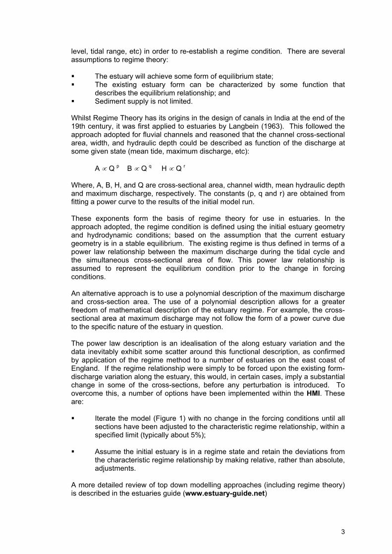
level, tidal range, etc) in order to re-establish a regime condition. There are several assumptions to regime theory: The estuary will achieve some form of equilibrium state; The existing estuary form can be characterized by some function that

describes the equilibrium relationship; and Sediment supply is not limited.

Whilst Regime Theory has its origins in the design of canals in India at the end of the 19th century, it was first applied to estuaries by Langbein (1963). This followed the approach adopted for fluvial channels and reasoned that the channel cross-sectional area, width, and hydraulic depth could be described as function of the discharge at some given state (mean tide, maximum discharge, etc):

A ∝ Q p B ∝ Q q H ∝ Q r Where, A, B, H, and Q are cross-sectional area, channel width, mean hydraulic depth and maximum discharge, respectively. The constants (p, q and r) are obtained from fitting a power curve to the results of the initial model run. These exponents form the basis of regime theory for use in estuaries. In the approach adopted, the regime condition is defined using the initial estuary geometry and hydrodynamic conditions; based on the assumption that the current estuary geometry is in a stable equilibrium. The existing regime is thus defined in terms of a power law relationship between the maximum discharge during the tidal cycle and the simultaneous cross-sectional area of flow. This power law relationship is assumed to represent the equilibrium condition prior to the change in forcing conditions. An alternative approach is to use a polynomial description of the maximum discharge and cross-section area. The use of a polynomial description allows for a greater freedom of mathematical description of the estuary regime. For example, the cross-sectional area at maximum discharge may not follow the form of a power curve due to the specific nature of the estuary in question. The power law description is an idealisation of the along estuary variation and the data inevitably exhibit some scatter around this functional description, as confirmed by application of the regime method to a number of estuaries on the east coast of England. If the regime relationship were simply to be forced upon the existing form-discharge variation along the estuary, this would, in certain cases, imply a substantial change in some of the cross-sections, before any perturbation is introduced. To overcome this, a number of options have been implemented within the HMI. These are: Iterate the model (Figure 1) with no change in the forcing conditions until all

sections have been adjusted to the characteristic regime relationship, within a specified limit (typically about 5%);

Assume the initial estuary is in a regime state and retain the deviations from

the characteristic regime relationship by making relative, rather than absolute, adjustments.

A more detailed review of top down modelling approaches (including regime theory) is described in the estuaries guide (www.estuary-guide.net)

3

1.4 Product Overview The software is open source code

The majority of the software has been written in the programming language

Visual Basic 6. Graphical plots available within the HMI have been created using the Matlab programming language (Version 2007a). Neither Visual Basic or Matlab is required by the user to install or run the HMI;

The code is annotated and designed to allow experienced programmers the

ability to alter or add code. Many of the routines have been written in a modular environment allowing experienced users to easily add or modify existing routines;

The software has been designed around a Microsoft Windows environment,

which allows for a familiar and easy to operate setting;

The HMI represents a standardised approach, thus enabling the user to apply regime theory to an estuary without the need to write bespoke software, which maybe subject to programming errors;

The software dynamically runs the following 1D models: Mike11 and

InfoWorks. The software combines regime theory with the process based hydrodynamic model to create a hybrid modelling approach. The dynamic approach means that complexity of extracting results from the process based model and interpretation into the regime equations has been solved without the need for user intervention;

A new estuary morphology is created based on the change or changes in the

forcing conditions within the estuary. The resulting bathymetry may be a representation of the new likely shape of the estuary. However, the new shape of the estuary is subject to a large degree of interpretation. This is because the morphology of the estuary is based on achieving the correct area/discharge relationship. The estuary shape is altered based on a set of parametric fits and not the physical conditions within the estuary, i.e. consideration of the threshold of motion. The new shape of the estuary is stored as either a Mike11 cross-section file or within the InfoWorks setup files;

The software calculates intertidal and plan areas, volumes, and hydraulic

information. Additional information is provided relating to the hydrodynamic and regime simulation. This information is exported as ASCII text files. Under the Mike11 software this information is broken down into individual network branches (if present);

A graphical user interface (GUI) has been developed to allow the user to view

and amend cross-sections;

An analysis of the tidal asymmetry (tidal excursion, net slack duration, slack gradient and Dronker’s asymmetry ratio) can be undertaken within the HMI;

The morphological tidal period can be determined within the HMI. This routine

calculates the theoretical period represented by a sequence of morphological tides. These tides alone are sufficient to enable longer-term (centuries to decades) simulations to be made; and

4

Energy calculation, an estimate of the 1D energy terms is provided.

1.5 What the HMI Interface Cannot Do!

Currently (Version 1.0.0) the HMI cannot simulate the following:

1.5.1 Waves The effect of waves has two main consequences for estuaries: Extra subtidal transport at the estuary entrance where wave action can be

significant; and

The evolution of the upper profile of intertidal areas that are governed largely by wave (local or swell) rather than current action.

The first effect (that of extra subtidal transport), is the cause for the shallowing and widening that occurs at estuary entrances (De Jong and Gerritsen, 1984). Transport from offshore and from littoral drift causes the shallowing but the combination of waves and currents means that a larger channel cross-section can be sustained (compared to an equivalent situation without waves). The development of a regime model that includes the influence of waves has not been implemented. Work by J. Spearman under the Defra project FD2116 (Review and formalisation of geomorphological concepts and approaches) highlighted the following equation based on shear strength at the bed:

21

maxmax ⎟⎟⎠

⎞⎜⎜⎝

⎛→ +

c

cwQQττ

Where: Qmax = Maximum Discharge;

cw+τ = Bed shear strength under waves and currents;

cτ = Bed shear strength under currents.

1.5.2 Sediment Under the research contract FD2116, two separate regime algorithms have also been proposed for sandy and muddy estuaries.

( )2211

Ki

Kiii QQ.aAA −=− ++ Sandy estuaries

⎥⎥⎦

⎤

⎢⎢⎣

⎡⎟⎟⎠

⎞⎜⎜⎝

⎛−⎟⎟

⎠

⎞⎜⎜⎝

⎛=− +

+

+++

m

E,i

iKi

m

E,i

iKiii C

CQ

CC

Q.aAA 1

1

111

22 Muddy estuaries

where Ci and Ci, E are the “representative” actual and equilibrium concentrations at a given cross-section at time-step i of the evolution; K2 is a function of p and q; and a is

5

a constant depending on the time-scale of interest, p and q are derived from the regime fit. Attempts were made to implement these algorithms but were unsuccessful. Specifically, the stability (the amount of change made to a cross-section) of the above approaches could not be resolved under this current phase of the Estuaries Research Program (ERP).

1.5.3 Bed Updating Under the current version 1.0.0 the bed updating is performed using a linear stretching approach. Consideration of the geological constraints is implemented (see Constraints), however, the variation in velocity (Figure 2) over the cross-section is not considered.

Figure 2. Changes in flow speed across a transverse profile

1.6 System Requirements A guide to the minimum requirements for running the HMI include (Mike11 and ISIS users): 200MHz Pentium PC;

128Mb memory minimum. 256Mb memory recommended;

Hard disk with 200Mb space available. Most master databases used for

serious modelling work will be larger than this. Some may be many times larger. You will need to regularly check that you have enough space;

1024x768 resolution, high-colour (16 or 24-bit) graphics card and screen. It is

easier to work with multiple windows open if you have as high a screen resolution as possible;

CD-ROM drive;

Windows 2000 or Windows NT 4.0 (or later versions);

The HMI can also be run on any standard Windows-based network, although

this may result in longer simulation times.

When modelling using a large number of cross-sections you may find that these minimum specifications result in unacceptably slow operation. A faster processor and more memory will provide the best performance improvements. Running over a network may also result in slow operational times. It is recommended that all simulations should be run from the local machine. Some additional tools and graphical components may not be available if operated over a network connection.

6

1.7 Installing the Hybrid Model Interface The user can run the HMI either through the program Visual Basic 6 or install the compiled Shell_Interface.exe file. To install the HMI the user should carry out the following steps: Double click on the setup.exe program, this will bring up an instillation screen as shown in (Figure 3), during the installation process. Follow the on-screen instructions.

Figure 3. Initial setup screen

It is recommended that you install the software in the default location: (C:\Program Files\Shell)

As part of the HMI program a number of additional tools have been provided. These have been written in the programming language Matlab. In order for these products to work the user must run the setup file MCRInstaller.exe (Figure 4). Once the user has installed the runtime components the MCRInstaller.exe file can be removed.

7

Figure 4. Matlab setup and installation program The MCRInstaller.exe file loads the Matlab graphical libraries and is required to show the GUI files written into the HMI.

The HMI does not require the user to install Matlab to run a regime simulation. However, the user will not be able to make use of the graphical routines.

From previous experience, GUI’s within the HMI do not appear to work successfully if running over a shared network drive. It is recommended that all modelling files be run from the local machine.

8

Part 2. Using the Hybrid Model Interface

2.1 Step One

2.1.1 Applies To All Models BACKUP ALL FILES, the HMI is designed to be as foolproof as possible. However, it is strongly recommended that you make a complete backup of all model files in case the program terminates unexpectedly resulting in a loss of model data files.

Prematurely ending from the HMI may corrupt some of the simulation files. If the HMI falls over the user should replace the cross-section file in the Mike11 simulation or exported ISIS .csv file from your backup copies!

2.2 Getting Started

2.2.1 Applies to All Models

The default installation process will have created an option in the Programme’s Shell Interface – Shell Interface (Figure 5) section of the Windows Start. Selecting this option will run the HMI program (Figure 6). Alternatively, if you have created an icon on the desktop, double-clicking on this icon will run the program. Alternatively, if you have Microsoft Visual Basic 6 software, it is better to run the HMI from within this environment. This gives the user many more benefits including the ability to step through the code and debug if and where necessary.

Figure 5. Selecting the HMI termed ‘Shell Interface’

9

Clicking on the central command button provides a list of hydrodynamic model options for the user to select. Also displayed is the version number for the software. Clicking on the web link will take the user directly to the ABPmer web site. From here the user can use the estuary guide that can provide additional information on regime modelling and the additional tools provided within the HMI.

Figure 6. The initial screen displayed in the HMI Due to the significant difference in the way the DHI (Mike11) and the Wallingford Software (InfoWorks) operate this manual describes both approaches where appropriate. For the processes identical to both numerical models only one description is given.

2.2.2 Mike11 Users Only Mike11 users will be prompted to select the location of the Mike11.exe. Typically, the default location for this is C:\Program Files\DHI\MIKEZero\bin\Mike11.exe file. Once you have selected this you will not be asked for its location again. The Mike11.exe path information is stored in the file RegimeControl.txt. This file is typically located in the same directory as the ShellInterface.exe file. The first time you select the DHI Mike11 model choice the HMI will ask you to point to the location of the Mike11.exe file (Figure 7).

Figure 7. Directory mapping location for Mike11.exe file Typically, the DHI Mike11 program is located in the following location: C:\Program Files\DHI\MIKEZero\bin\mike11.exe. The HMI will create a text file RegimeMike11Control.txt that is used to point to the Mike11.exe file.

10

Changing the location of the Mike11.exe file after installing and running the HMI for Mike11 will cause a run time error. The user must either edit the directory information in the RegimeMike11Control.txt file or delete this file completely.

2.3 Model Simulation - Initial Setup Conditions

2.3.1 Applies To All Models

The first step in running a regime simulation is to verify the correct setup of the hydrodynamic model. In order to perform a regime analysis the assumptions (described in Section 2.3.2 Assumptions) MUST be true. If the user is happy that the system in question can be defined by a regime analysis then an existing or baseline scenario is required. This existing simulation represents the system before any perturbation has been introduced. A further run scenario may also be required, this run simulation is identical to the baseline model except that the run simulation represents some change to the system. Typically, this perturbation is a change in the boundary conditions, model bathymetry or the inclusion of storage areas.

A run scenario simulation may not be required if the user is interested in adjusting the existing condition to an idealised state. See Defining a Regime State.

2.3.2 Assumptions

The existing system can be characterized by a regime condition (see

Section 1.3, What is Regime Theory?);

Waves are not significant. Environments where waves play a significant role in the morphology of the estuary cannot be simulated in this approach;

The system has sufficient sediment to allow accretion to occur; and

The hydrodynamic model is calibrated (i.e. water levels, bathymetry

and flows are correctly represented in the model).

An estuary is considered to be in equilibrium when there is no or negligible net sediment movement over a long period of time at any place, neglecting seasonal variation

Before running the HMI an existing (baseline) simulation is required. The user must ensure that the model simulation files have the following setup conditions and have been successfully run within the hydrodynamic modelling software without generating errors.

Try to ensure the model is as stable as possible i.e. try reducing the model time-step or reducing the number of cross-sections within the model. This will ensure the process of running the regime analysis will be less likely to crash due to model instabilities

11

2.4 Model Boundary - Initial Setup Conditions

2.4.1 Applies To All Models An underlying regime assumption is that the estuary can be characterized by a regime relationship during a peak event (discharge or velocity). Therefore, careful consideration is required as to the particular water level boundary condition to apply. A tidal period that is not representative of the estuary will produce an incorrect prediction of the existing and future regime states of the estuary. For running a regime simulation, typically, a mean spring tide is chosen, where only a single tide is simulated (See Section 2.4.2 Flood Ebb Dominance for selecting the specific tidal period). Since the regime model only requires the peak event, short simulation periods are adequate. In the section Morphological Tides, the option of selecting a tidal period from a longer time-series is discussed. Here the user can select the specific tide(s) used to undertake the regime analysis. For analysis of tidal asymmetry, energy and morphological tides (these are discussed later) the user will need to run a simulation for at least several tides.

There may be a period of instability at the start of the model simulation. The length of the simulation needs to take this ‘Warm-up Period’ into account. Therefore, it is a good idea to run for at least 1 more tidal cycle depending on the size of your model!

To prevent any instability at the start of the simulation being considered in the regime analysis the user can define a period at the start of the time-series, which the HMI software will ignore (Figure 8). Example: 300 time-steps in the result file simulation; each time-step represents

a period of 10mins. An initial period of instability (‘Warm up’) lasts for approximately 2 hr, therefore the user sets the ‘Change Start Time-Step’ (Figure 8).

The HMI by default will ignore the first 20 time-steps. This is highly dependent on the individual model simulation and the user should ensure they set this value depending on the length of the output and stability of the simulation.

12

The user can specify the start time step in the result time-series file under the Data menu option

Figure 8. The read baseline hydrodynamic control form

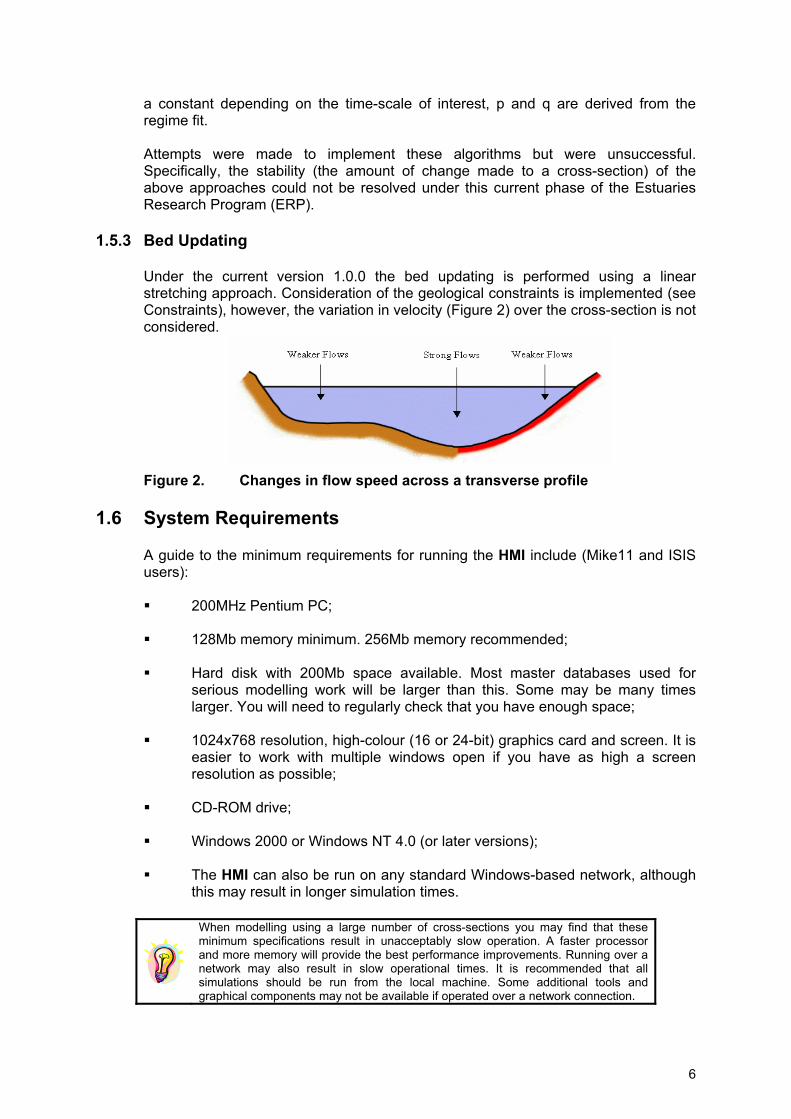
2.4.2 Flood or Ebb Dominance It is important that the user understands the flood or ebb dominance within the particular estuary they are studying. For example (Figure 9) shows a water level and 2 points of maximum discharge (baseline and scenario). In this example, the scenario simulation may represent only a small change in the system i.e. 1mm change in mean sea level (msl), however, because the dominance has switched (from flood to ebb or vice versa) the potential difference in water level can be large. Typically, this results in changes in cross-sectional area occurring in those cross-sections that may be expected to show no or very little change.

An examination of the result files WaterLevel_Data_n.txt from the HMI for the baseline and scenario files provide an indication to the user of these potential errors. These are saved in the Output_Files folder in the VB directory

For the estuary under investigation the user is advised to run for just a flood or ebb tidal period only. The user should consider the variation between the maximum discharge and velocity for a flood or ebb tide, the user is advised to select that part of the tide, which shows the largest discharge.

13

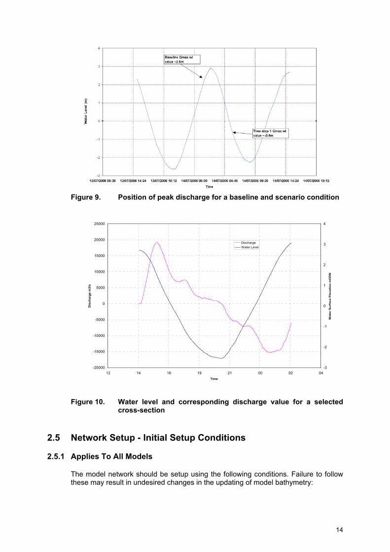
Figure 9. Position of peak discharge for a baseline and scenario condition

-20000

-15000

-10000

-5000

0

5000

10000

15000

20000

25000

12 14 16 19 21 00 02 04Time

Dis

char

ge m

3/s

-3

-2

-1

0

1

2

3

4

Wat

erSu

rfac

eEl

evat

ion

mO

DN

DischargeWater Level

Figure 10. Water level and corresponding discharge value for a selected

cross-section

2.5 Network Setup - Initial Setup Conditions

2.5.1 Applies To All Models The model network should be setup using the following conditions. Failure to follow these may result in undesired changes in the updating of model bathymetry:

14

The model network should start at zero chainage from the Mouth of the estuary. Many of the calculation routines assume that the first cross-section is at the mouth, reversing this order may result in errors;

The network may have multiple branches (Figure 11); and

Each branch should have a unique name. Do not use only numbers as

branch names, e.g. Branch 1, Branch 2.

Figure 11. HR Wallingford ISIS model of Tollesbury Creek

15

2.6 Cross-Section File - Initial Setup Conditions

2.6.1 Applies To All Models

Figure 12. Cross-sections (black lines) defined within Southampton Water

The cross-section file must NOT contain unused cross-sections;

Avoid overlapping of cross-sections (Figure 12);

The cross-section chainage MUST be whole numbers; the chainage length

values for each cross-section must NOT have decimal places. There are a number of tests within the software that do not apply to chainage values with decimal places;

Avoid using negative chainage values in the cross-section bathymetry and

branch chainage values. With the exception of depth (z) values, ensure all values within the cross-section file are positive;

Each section should have sufficient points to describe the geometry of the

section, in particular the intertidal zone (Figure 14). The update routine becomes unstable when the spacing between points describing the cross-section is too great. As a rule of thumb, typically the spacing across a large cross-sections with top-widths greater than 1-2km is 30-50m. For cross-sections with a top width less than 1km a 5-20m spacing between points;

The cross-sections MUST extend beyond the point of maximum high water.

Do not be worried about extending the cross-sections well beyond the high water line. This ensures that the model will remain stable during the numerous morphological adjustments. However, ensure suitable corrections are made to the profile if the elevations behind the maximum water level

16

position are below the maximum water line as shown by the yellow area in (Figure 13);

A maximum of 10 channels are allowed within a cross-section profile. A

channel is defined where the water elevation is below the land elevation at either peak discharge or peak velocity;

Within the HMI code, all elements start at array number 0. Therefore, cross-

Section 1 is Element 0.

Highlighted area has been artificially adjusted. No erosion can occur if

constrained by underlying geology or coastal defence

Maximum water level

Figure 13. Amended section profile

Extending the cross-sections too far beyond the high water line may cause errors in the flow calculations. If ponds are described behind the high water or coastal defence line then these may be used in the flow calculation causing increased flow. Ensure low lying elevations behind coastal defences are either removed or artificially increased (Figure 13).

17

High-resolution bathymetry along the intertidal section of the cross-section profile

Figure 14. Resolved cross-section profile

Higher resolution data is added in the cross-section profile between low water and the high-water position. This allows for a smoother adjustment of the cross-section.

Avoid cross-section profiles that have a large amount of data scatter (Figure 15), where the bathymetry jumps in elevation. These areas, particularly found along the intertidal margins, cause instabilities within the update procedure. To avoid instabilities in the modelling it is recommended that the user ‘smoothes’ out these areas, using the mean value.

18

Water level at peak discharge

Potential sea defence wall

Intertidal areas have been poorly defined. These areas should be avoided.

Figure 15. An example of a cross-section profile with a high degree of bathymetry scatter along the intertidal margins

2.7 Output Settings 2.7.1 Mike11 Users Only

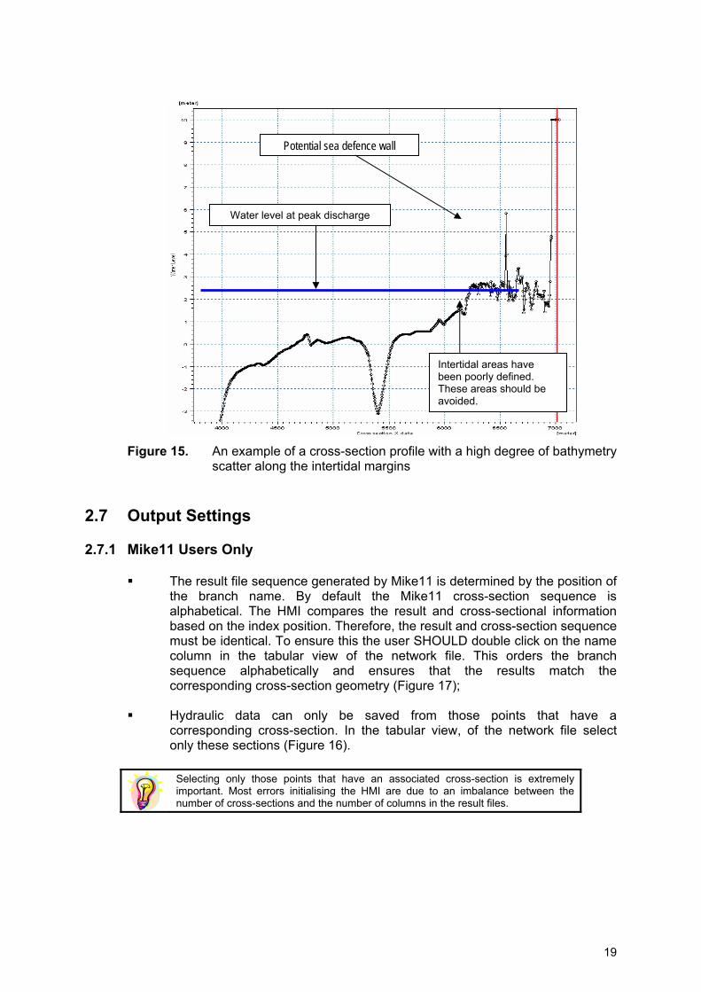
The result file sequence generated by Mike11 is determined by the position of

the branch name. By default the Mike11 cross-section sequence is alphabetical. The HMI compares the result and cross-sectional information based on the index position. Therefore, the result and cross-section sequence must be identical. To ensure this the user SHOULD double click on the name column in the tabular view of the network file. This orders the branch sequence alphabetically and ensures that the results match the corresponding cross-section geometry (Figure 17);

Hydraulic data can only be saved from those points that have a

corresponding cross-section. In the tabular view, of the network file select only these sections (Figure 16).

Selecting only those points that have an associated cross-section is extremely important. Most errors initialising the HMI are due to an imbalance between the number of cross-sections and the number of columns in the result files.

19

Figure 16. Save results from the cross-section positions only

In the Tabular View of the Mike11 Network, under branch name, if more than 1 branch exists then the user must double click on this column to sort in alphabetical order

Figure 17. Correctly ordering the output from the Mike11 model

2.8 Hydrodynamic File - Initial Setup Conditions

2.8.1 Mike11 Users Only

In the Mike11, Hydrodynamic file additional parameters tab (Figure 18), the user MUST select the following additional output parameters: Discharge *

Additional Parameters *

Velocity * Top-width * Area * Water levels (included by default, however these are not output in the

additional parameters tab).

20

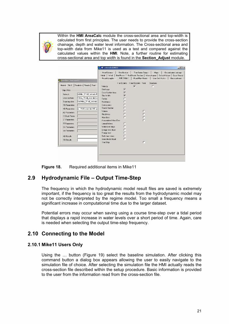
Within the HMI AreaCalc module the cross-sectional area and top-width is calculated from first principles. The user needs to provide the cross-section chainage, depth and water level information. The Cross-sectional area and top-width data from Mike11 is used as a test and compared against the calculated values within the HMI. Note, a further routine for estimating cross-sectional area and top width is found in the Section_Adjust module.

Figure 18. Required additional items in Mike11

2.9 Hydrodynamic File – Output Time-Step The frequency in which the hydrodynamic model result files are saved is extremely important, if the frequency is too great the results from the hydrodynamic model may not be correctly interpreted by the regime model. Too small a frequency means a significant increase in computational time due to the larger dataset. Potential errors may occur when saving using a course time-step over a tidal period that displays a rapid increase in water levels over a short period of time. Again, care is needed when selecting the output time-step frequency.

2.10 Connecting to the Model

2.10.1 Mike11 Users Only Using the … button (Figure 19) select the baseline simulation. After clicking this command button a dialog box appears allowing the user to easily navigate to the simulation file of choice. After selecting the simulation file the HMI actually reads the cross-section file described within the setup procedure. Basic information is provided to the user from the information read from the cross-section file.

21

Figure 19. Baseline Mike11 simulation form

The initial calculation of cross-sectional area and top width is based on a water elevation of 5m. The value of 5m is arbitrary and only assigned to provide the user an indication of the relative differences in the cross-sectional areas.

2.10.2 InfoWorks Users Only After selecting the InfoWorks (ISIS) model the user is taken to the Read Baseline InfoWorks Simulation form. This form is designed to allow the user to enter information regarding the existing baseline model. As described in the section Setting-up the Existing Baseline Model Simulation, the baseline model represents the system before any perturbation. The user must first tell the HMI software the file locations and model simulation names. The HMI then runs a number of procedures that call the InfoWorks model and extracts the model bathymetry and hydrodynamic information (Figure 20).

22

Figure 20. Baseline InfoWorks simulation form

2.10.3 InfoWorks Folder and File Structure

The following folder/file and simulation data is required in each field of the baseline InfoWorks simulation form: InfoWorks File Name - This is a *.iwm file; Local Root - The local directory; Export Folder - The export folder name; Results Folder - The result folder name; Import File Name - The import file name.

The file/folder information can be entered using the command buttons as shown below. If there is an error with this information the InfoWorks program will report an error.

An easier way to provide the correct data is by opening the InfoWorks RS module. The names of the simulation data can be read and then entered into this form.

2.10.4 Save and Load InfoWorks Setup Information

The user can save and load the InfoWorks ISIS setup information from an existing file. By clicking Load or Save on the Baseline InfoWorks Simulation Form, a common

23

dialog box appears (Figure 21) allowing the user to navigate to the selected file and location. After the InfoWorks information has been entered into the HMI, the user must then initialise the program (Figure 22).

Figure 21. Using the Load and Save functions to store and retrieve the simulation

setup parameters

2.10.5 Initialise the Model Once the model simulation data has been entered into the InfoWorks setup form, the user must initialise the model (Figure 22). Initialise means that the InfoWorks model is capable of communicating with the ISIS hydrodynamic simulation.

Initialise the InfoWorks model by clicking on the control button. This should be done only after all the fields have been completed.

Figure 22. Baseline InfoWorks simulation form

Entering incorrect names generates errors from the InfoWorks Com object. The reported errors may not be fully explained. Errors encountered during this part of the procedure are typically due to bad field names. If errors are reported check that you have entered the path and file names correctly

24

The model simulation such as Network, Model, Run names and so on are required to establish the correct link to the InfoWorks (ISIS) model. Information incorrectly entered here will generate an error from the InfoWorks software and the user will be unable to proceed. Some additional help is provided with many of the controls. By hovering with the mouse cursor over the text field or command button a description of the information required is provided

2.11 Changing the Bathymetry

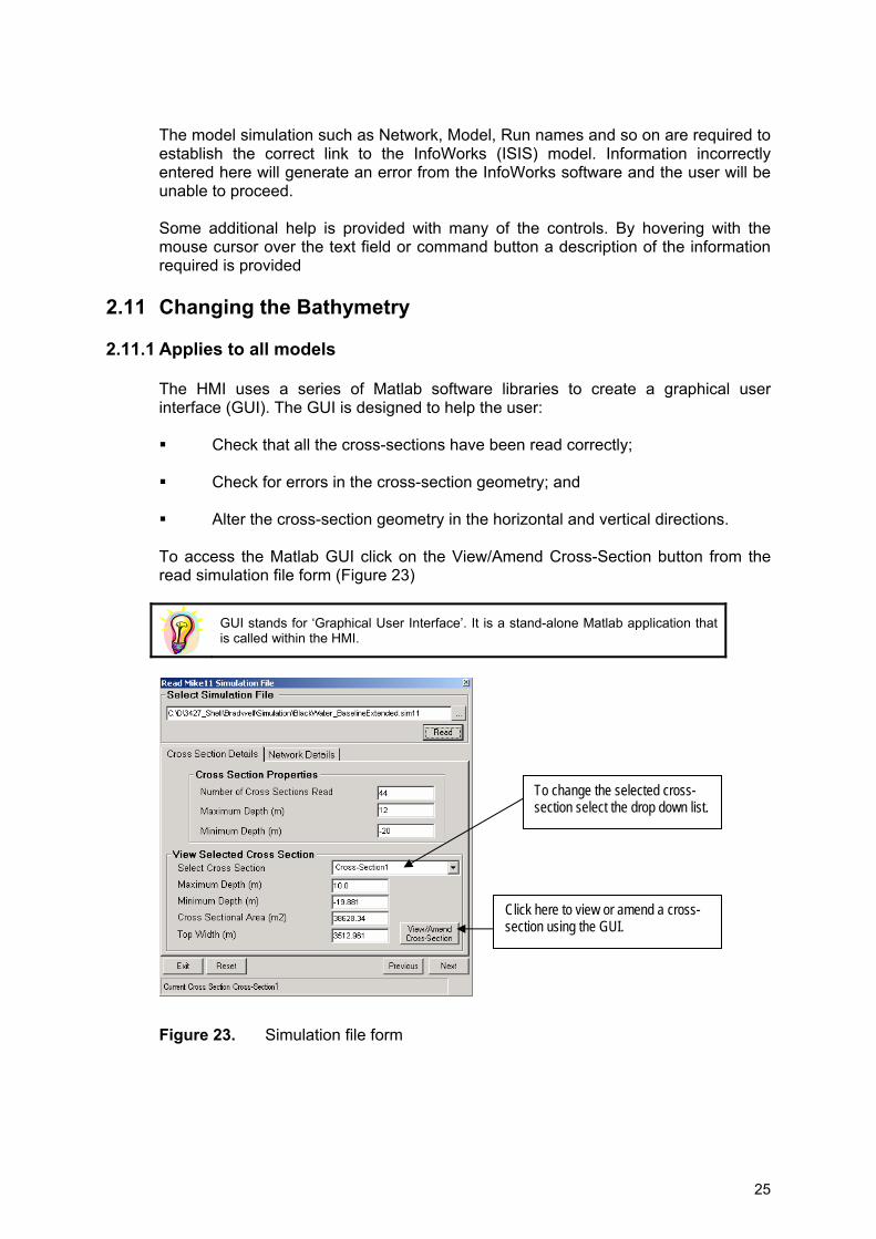
2.11.1 Applies to all models The HMI uses a series of Matlab software libraries to create a graphical user interface (GUI). The GUI is designed to help the user: Check that all the cross-sections have been read correctly;

Check for errors in the cross-section geometry; and

Alter the cross-section geometry in the horizontal and vertical directions.

To access the Matlab GUI click on the View/Amend Cross-Section button from the read simulation file form (Figure 23)

GUI stands for ‘Graphical User Interface’. It is a stand-alone Matlab application that is called within the HMI.

To change the selected cross-section select the drop down list.

Click here to view or amend a cross-section using the GUI.

Figure 23. Simulation file form

25

2.11.2 Editing a Single Point

To edit a single point using the GUI the user should carry out the following steps:

1) Select ‘Single Point’ from the ‘Select edit method’ dialogue box (Figure 24);

2) Using the mouse click on to the selected point (the user may need to zoom if

the cross-section points are situated very close);

3) The selected point will be highlighted in red; and

4) The user can either drag the point to the new location or manually enter the new horizontal and vertical position.

The user can select another point with the mouse or click ‘Save Changes’ to close the form and write the new cross-section data back to the HMI. Alternatively, the user can decide not to save the changes by simply clicking the close command button. For Mike11 users - the cross-section information is saved in the external ‘.xns11’ file after closing the GUI.

The Pan, Zoom and Save functions allow the user to manipulate the plot.

Select the Single Point edit method (default) to alter or amend a single point along the cross-section

The co-ordinate position can be manually entered for a single point

Figure 24. Matlab generated GUI

2.11.3 Editing Multiple Points To edit multiple points using the GUI the user should take the following steps: 1) Select ‘Multiple Points’ in the ‘Select edit method’ dialogue box (Figure 25);

2) Using the mouse click once on to a point outside the area you wish to change

(the user may need to zoom if the cross-section points are situated very

26

close). Moving the mouse will cause a hashed box to appear. Once the area that the user would like to alter is enclosed by the box, click again;

3) The selected points will be highlighted in red;

4) Using the mouse, the user can drag the selected points to the new location

then release the mouse button to assign the position of the selected points. For reference, the previous positions of the selected points are indicated by faint blue positions on the interface; and

5) Additional points can be selected by following Step 1 to 3. The user can either

decide to save the new cross-section geometry by pressing the save changes button or disregard the changes by pressing the close button.

The GUI is NOT designed as a complete substitute for the existing routines within the (DHI or InfoWorks) models. Consider the GUI as an aid in order to make simple or routine adjustments

Select the Multiple Point edit method to alter or amend more than 1 point along the cross-section Left mouse click once to define the start of the rectangle and again to define the finish. Drag the highlighted points to the

Figure 25. Matlab cross-section editor GUI The user cannot perform the following applications within the GUI: Add new cross-sections; Change the position of the cross-section along the branch; and Change the ID or name of the cross-section.

2.11.4 Mike11 Users Only

After selecting the Mike11 model option from the Hydrodynamic Model Selection screen the user is asked to select the existing baseline simulation. When the Mike11

27

simulation file has been read correctly the View Cross-Section button will become available. By clicking this button the GUI is opened.

If the user decides to save the file in the GUI the Mike11 cross-section file will be over written. The user should make sure they wish to keep these saved changes.

2.11.5 InfoWorks Users Only

In the InfoWorks simulation the information regarding the cross-sections are saved internally. No immediate updates of the cross-sections are performed.

2.12 Reading the Hydrodynamic Data After selecting and reading the Simulation File, the user is requested to supply the Hydrodynamic Results file (1D model output in the form of a. res11 file (for Mike-11) or a *.dat file (for ISIS)). The hydrodynamic data is read and stored internally. These internal variables hold the hydrodynamic data that is in turn applied throughout the program. Typically, the internal variables are defined in the module RegimeVariables.mod.

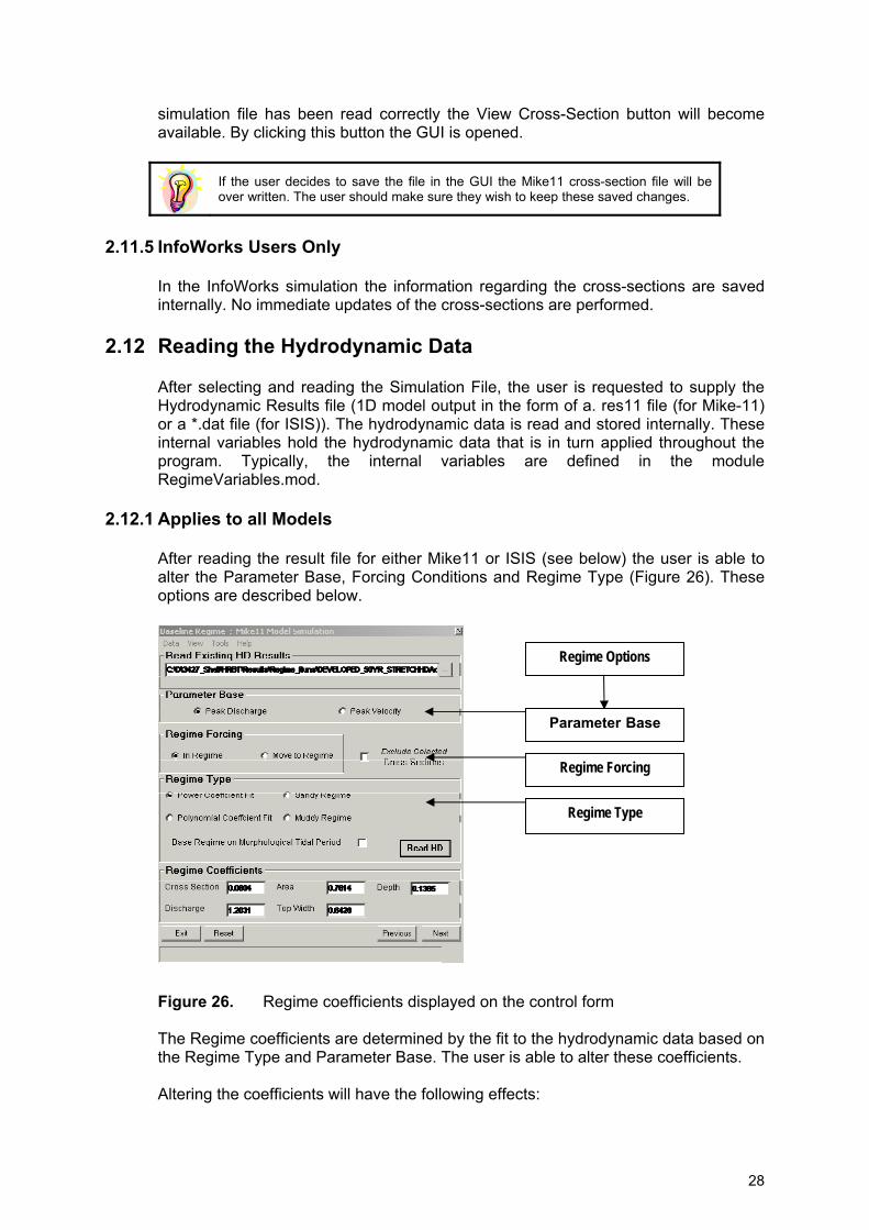
2.12.1 Applies to all Models After reading the result file for either Mike11 or ISIS (see below) the user is able to alter the Parameter Base, Forcing Conditions and Regime Type (Figure 26). These options are described below.

Regime Options

Parameter Base

Regime Forcing

Regime Type

Figure 26. Regime coefficients displayed on the control form

The Regime coefficients are determined by the fit to the hydrodynamic data based on the Regime Type and Parameter Base. The user is able to alter these coefficients. Altering the coefficients will have the following effects:

28

Top Width: By increasing this value the cross-sections will increase the amount of width adjustment. Equally, reducing this value will reduce the amount of horizontal adjustment to each cross-section. Note, it might be required to devise a spatially varying top width coefficient if sufficient knowledge is known about the system in question; and

Depth: By increasing this value the cross-sections will increase the amount of

depth adjustment. Equally, reducing this value will reduce the amount of vertical adjustment to each cross-section.

It is not recommended to alter the following parameters.

2.12.2 Parameter Base The user can select to base the regime condition on the relationship between cross-sectional area and either peak discharge or peak velocity. Typically, the relationship between cross-sectional area and peak discharge is preferred, i.e. the behaviour of the estuary is better described by this comparison than between peak velocity and cross-sectional area. The regime parametric fits are compared against either maximum discharge or peak velocity. The HMI analyses the time-series selected by the user and selects and stores the maximum discharge or velocity at each cross-section within the hydrodynamic model. At the corresponding time-step the top-width and cross-sectional area are determined and stored.

By default Peak Discharge (Peak Q) is recommended as this typically provides a better fit to the estuary.

2.12.3 Regime Forcing

Regime theory assumes that the estuary is in a regime condition. By this it is assumed that the cross-sectional area at peak discharge or velocity is in a regime condition. (Figure 27) shows the relationship between maximum discharge and the corresponding cross-sectional area. Maintaining this ‘Regime’ relationship is the basis of the modelling approach. Note in Figure 27, there is some scatter in the data, this is typical of many estuaries, the consequence of this scatter is discussed next.

29

Figure 27. Regime fit (Cross-section area vs Maximum discharge) By selecting the ‘In Regime’ option the user assumes that the scatter away from the idealised line is acceptable (Figure 27). Internally the HMI will modify the cross-sections after an introduced perturbation thus ensuring that the final cross-sectional area vs. discharge relationship will be an equal distance away from an idealised regime state. The theory behind this key assumption is described below. The coefficients of the regime equation are incorporated in the expression

QE = aAb Where:

QE = the equilibrium discharge m3/s A = the cross-sectional area at equilibrium discharge m2 (a, b) = coefficients to be solved from the hydrodynamic model run used to

construct the regime solution. The model is run for a tidal cycle and the maximum flow rates QE(x) and the cross-sectional areas of flow A(x) associated with them, at each cross-section in the model, are retained. QE is then fitted through the data by a regression procedure, to obtain the coefficients (a, b):

Y = α + b·x

loge(QE) =loge(a) + b·loge(Area) However, if the regime model were now to be run, with spatially constant values of (a, b), under the bathymetric conditions that were used to derive those two coefficients, the model would not be in equilibrium and it would attempt to update the cross-sections until they fitted to obtain coefficients (a, b) throughout the system. It has been found that this effect would in general be especially pronounced at the

The red line indicates the theoretical ‘regime’ state for the estuary. The blue dots show how far the individual cross-

30

upstream end of the model, although it would propagate throughout the model, with repeated iterations. If it is assumed that the model is in regime at the time that the two regime coefficients (a, b) are derived, then no changes should occur, if the regime model is run with these coefficients, under existing conditions. In order to ensure that this criterion was satisfied, the coefficient a was made spatially varying, that is, after obtaining the constant value of b the coefficient a was obtained by back-substitution:

a(x) =QE(x)/Area(x)b Overall, the variation in a(x) does not depart greatly from the constant value obtained to obtain the coefficients (a, b) except at the upstream end of the model, but it does provide a level of control over the model behaviour, to ensure that it is stable under existing conditions, in situations where these are deemed to represent a regime. Applications where the spatially-varying solution for the coefficient a is applicable, could be when the model is to be used for predicting the change in regime behaviour due to the implementation of a scheme, or due to a rise in sea level. In this case, the system is initially assumed to be stable, and all sectional changes that occur during the regime model run, can be effectively attributed to the physical changes imposed upon the system. Selecting the ‘Move to Regime’ option will move the cross-sections to this idealised line (move the points to the red line Figure 27). Effectively the cross-sectional area will be adjusted so that each point will lie on this regime state.

The ‘In Regime’ option is recommended; selecting the ‘Move to Regime’ may result in large changes in cross-sectional area without any change in the forcing of the system.

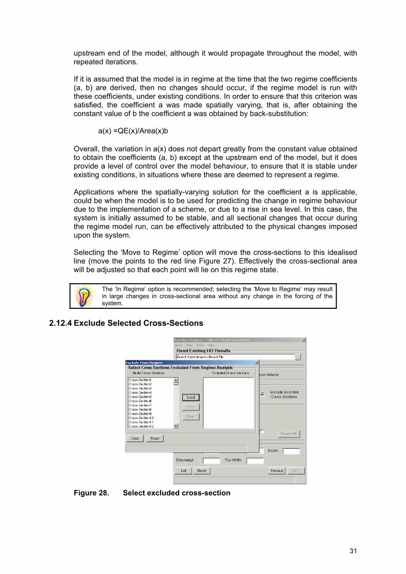
2.12.4 Exclude Selected Cross-Sections

Figure 28. Select excluded cross-section

31

Selecting the ‘Exclude Selected Cross-sections’ (Figure 28) button will display the ‘Exclude from Regime’ form with a complete list of the cross-sections used in the simulation. Note, as described earlier, redundant sections or sections not used in the model simulation but still present in the cross-section (.xns11) file or setup files are not permitted and will generate errors. The user can select the cross-sections they wish to exclude by double clicking on the selected cross-section in the list box. The selected cross-section will appear in the excluded cross-section list box. Alternatively, the user can load a pre-defined list of excluded cross-sections from an external file. The file should be in the following format with no headings or text (figure 29). The numbers listed in the file represent the cross-section sequence number and not the name or other ID for the cross-section:

2 10 20 21

Figure 29. Example of file format needed to exclude cross-section The user has the option to save the selected excluded sections to an external text file. Note, the user can also use this saved file to exclude sections from any morphological update, see ‘Defining the Regime Options’.

In the HMI the cross-section numbering starts from 0. Therefore the first cross-section will have a index number of 0. If the user wishes to excluded the first cross-section using the excluded cross-section files they must use 0, the second section has an index number of 1 and so on.

Excluding the selected cross-sections using the method described above will only prevent these excluded sections being analysed using the regime equations. Unless specified by the user these sections will be included in the cross-section update routines.

The user can save the cross-sections to be excluded using the save button (Figure 28). The user can also use this same file when excluding files in the update routine (see Exclude Selected Cross-sections)

2.12.5 Regime Type

Power Regime refers to a description of the estuary using a power coefficient fit to the hydrodynamic data. The power law description is defined by the equation:

Log(Q1) = b⋅log(AQ) + log(a) = a.AQb Where Q1 = Maximum discharge at a given cross-section and the discharge that is deemed to be commensurate with the specified regime, for a given simultaneous cross-sectional area.

The Power Regime description of the estuary is the classical approach and is recommended. The Polynomial description may be applied if there is significant scatter of in the data, although, previous studies have not shown a significant improvement using this approach

32

Polynomial regime

Log(Q1) = a⋅[log(AQ)]2 + b⋅[log(AQ)] + c The polynomial regime describes the fit between the peak discharge or velocity and the cross-sectional area, top width and hydraulic depth. The advantage of the polynomial description lies in the extra degree of freedom provided by the additional term c. The user may select to use the polynomial description when large changes in the predicted estuary morphology occur when the user selects the traditional power law relationship.

2.13 Existing Data Information Data from previous simulations is stored in the folder Matlab\Output_Files\.. Once the user clicks the Read HD command button an internal routine is called to delete existing simulation data from the stored folder location. A dialog box will appear asking whether this information can be deleted at the start of the current simulation (Figure 30).

Figure 30. Dialog box asking the user if the information contained within the

specified folder structure can be deleted

It is good practice to ensure that all hydrodynamic model and result files are backed up before the start of any new simulation. This must include results from the HMI program.

33

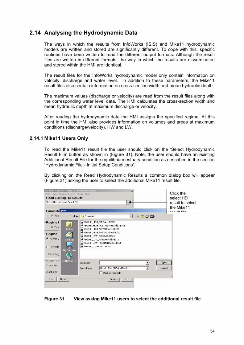
2.14 Analysing the Hydrodynamic Data The ways in which the results from InfoWorks (ISIS) and Mike11 hydrodynamic models are written and stored are significantly different. To cope with this, specific routines have been written to read the different output formats. Although the result files are written in different formats, the way in which the results are disseminated and stored within the HMI are identical. The result files for the InfoWorks hydrodynamic model only contain information on velocity, discharge and water level. In addition to these parameters, the Mike11 result files also contain information on cross-section width and mean hydraulic depth. The maximum values (discharge or velocity) are read from the result files along with the corresponding water level data. The HMI calculates the cross-section width and mean hydraulic depth at maximum discharge or velocity. After reading the hydrodynamic data the HMI assigns the specified regime. At this point in time the HMI also provides information on volumes and areas at maximum conditions (discharge/velocity), HW and LW.

2.14.1 Mike11 Users Only To read the Mike11 result file the user should click on the ‘Select Hydrodynamic Result File’ button as shown in (Figure 31). Note, the user should have an existing Additional Result File for the equilibrium estuary condition as described in the section ‘Hydrodynamic File - Initial Setup Conditions’. By clicking on the Read Hydrodynamic Results a common dialog box will appear (Figure 31) asking the user to select the additional Mike11 result file.

Figure 31. View asking Mike11 users to select the additional result file

Click the select HD result to select the Mike11 result file

34

In a Mike11 simulation the results files (*.res11) are stored as binary output. The HMI converts these files to ascii text using the Res11read.exe routine supplied by DHI.

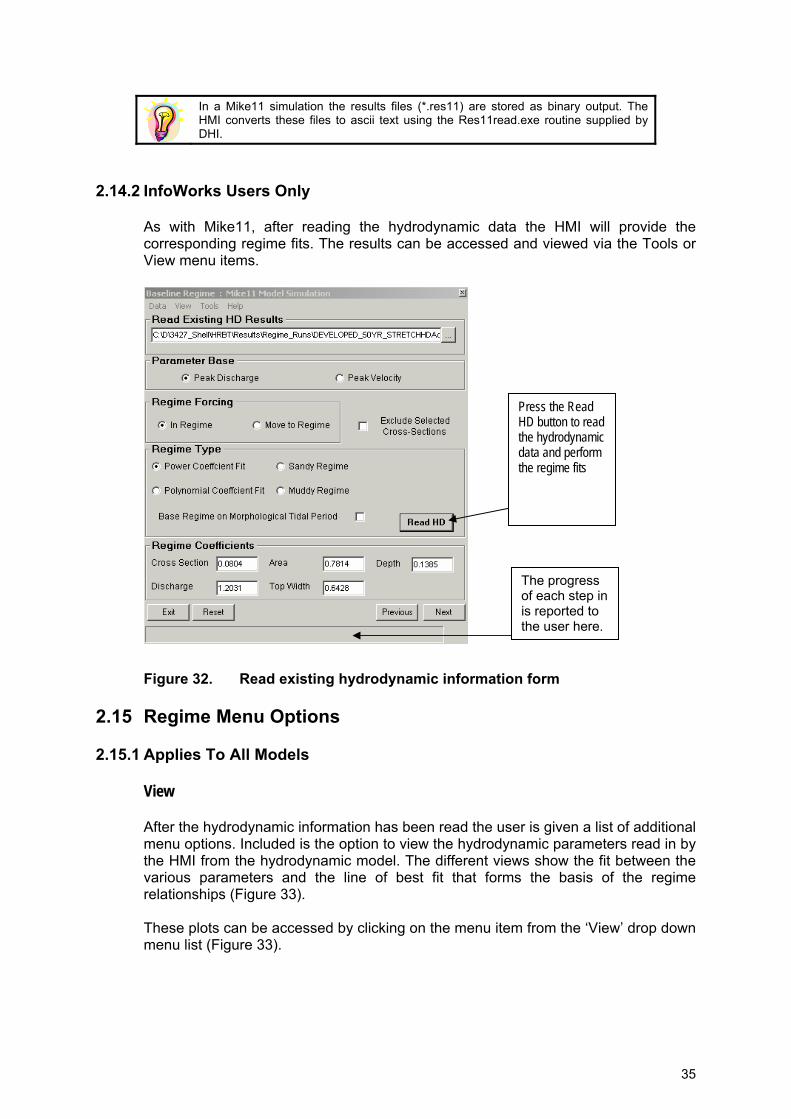
2.14.2 InfoWorks Users Only As with Mike11, after reading the hydrodynamic data the HMI will provide the corresponding regime fits. The results can be accessed and viewed via the Tools or View menu items.

Figure 32. Read existing hydrodynamic information form

2.15 Regime Menu Options

2.15.1 Applies To All Models

Press the Read HD button to read the hydrodynamic data and perform the regime fits

The progress of each step in is reported to the user here.

View After the hydrodynamic information has been read the user is given a list of additional menu options. Included is the option to view the hydrodynamic parameters read in by the HMI from the hydrodynamic model. The different views show the fit between the various parameters and the line of best fit that forms the basis of the regime relationships (Figure 33). These plots can be accessed by clicking on the menu item from the ‘View’ drop down menu list (Figure 33).

35

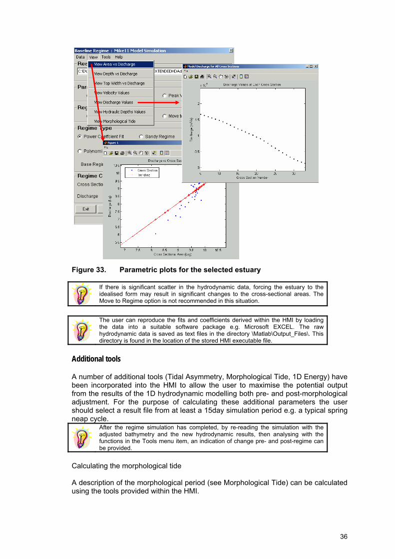
Figure 33. Parametric plots for the selected estuary

If there is significant scatter in the hydrodynamic data, forcing the estuary to the idealised form may result in significant changes to the cross-sectional areas. The Move to Regime option is not recommended in this situation.

The user can reproduce the fits and coefficients derived within the HMI by loading the data into a suitable software package e.g. Microsoft EXCEL. The raw hydrodynamic data is saved as text files in the directory \Matlab\Output_Files\. This directory is found in the location of the stored HMI executable file.

Additional tools A number of additional tools (Tidal Asymmetry, Morphological Tide, 1D Energy) have been incorporated into the HMI to allow the user to maximise the potential output from the results of the 1D hydrodynamic modelling both pre- and post-morphological adjustment. For the purpose of calculating these additional parameters the user should select a result file from at least a 15day simulation period e.g. a typical spring neap cycle.

After the regime simulation has completed, by re-reading the simulation with the adjusted bathymetry and the new hydrodynamic results, then analysing with the functions in the Tools menu item, an indication of change pre- and post-regime can be provided.

Calculating the morphological tide A description of the morphological period (see Morphological Tide) can be calculated using the tools provided within the HMI.

36

The user is given the option to calculate the morphological tidal period. Typically this period should be used when running either for the Sandy or Muddy regime types. These particular regime equations consider the potential sediment transport over some morphological time period. The use of the morphological tide allows the user to multiply the results from a single ‘representative’ morphological tide to predict the likely bed changes over longer time-scales. It is NOT possible to calculate the morphological tidal sequence unless the simulation runs over at least three tides. To calculate the morphological tidal period from the entire simulation period, the user should click on the Tools - Generate Morphological Tide option from the menu item as shown in (Figure 34).

Figure 34. ‘Generate Morphological Tide’ tool

The period highlighted by the red crosses (Figure 34) indicates the time over which either the simulation should be run or in which, the regime calculations can be calculated. The user can find this morphological tide by opening the text file \Matlab\Output_Files\ MorphTide.txt. Within the file example (Figure 35) the text highlighted in red denotes the selected morphological period, based on the velocity information for cross-section ID number 3. The selected marker for the morphological period is set to 1, the time frame outside of the selected morphological tide(s) has a marker value of 0.

37

Cross-Section ID, Velocity, Selected Period 3, 0.251, 0 3, 0.299,1 3, 0.324,1 Morphological period

indicated by the value 1. A value of 0 represents the non-morphological tidal sequence.

3, 0.224, 0

Figure 35. An example of the output format generated when the user calculates the morphological tide

By selecting the whole time-series and Column 3 the user can determine the morphological period condition by comparing this against the corresponding boundary file time-series. Select the part of the time-series with a 1 and use this as your new boundary file. Be aware that the start of the time-series has not been included in the morphological tide calculations to avoid the model warm-up, therefore, you must take this period into account when looking at the boundary file time-series.

The output file “MorphTide.txt” is based on a cross-section close to the mouth of the estuary. This is based on the assumption that the user must number the cross-sections from the mouth of the estuary working upstream. The user does not have the option to specify the cross-section in which to analyses the morphological tidal sequence. However, a close examination of the source code should allow the user to alter this if required.

To save time the user should re-run the hydrodynamic simulations over part of the calculated morphological tidal sequence as discussed in the section Flood or Ebb Dominance.

Base regime on morphological tidal period By selecting the ‘Base Regime on Morphological Tidal Period’ option the HMI will attempt to calculate the Morphological Period from the whole simulation. The regime and results from subsequent model iterations will be determined only from this period. Higher discharge and velocity values that occur in the simulation but outside this morphological period will be ignored. This functionality was originally included to accommodate the proposed regime algorithms developed as part of the Defra project FD2116 Review and formalisation of geomorphological concepts and approaches. However, under the present scope of work these additional algorithms have not been implemented. Although this option still exists its use is NOT RECOMMENDED The morphological tide data can be accessed from within the HMI ‘\Output_Files’. This is found in the installation path - typically ‘C:\Program Files\shell\vb\Matlab\Output_Files\ MorphTide.txt’ The file MorphTide.txt (Figure 36) contains the data used in the plots from the asymmetry analysis.

38

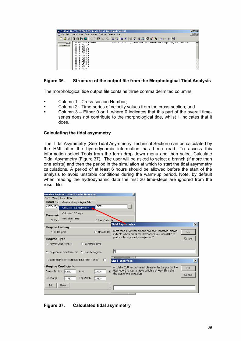
Figure 36. Structure of the output file from the Morphological Tidal Analysis The morphological tide output file contains three comma delimited columns. Column 1 - Cross-section Number; Column 2 - Time-series of velocity values from the cross-section; and Column 3 – Either 0 or 1, where 0 indicates that this part of the overall time-

series does not contribute to the morphological tide, whilst 1 indicates that it does.

Calculating the tidal asymmetry The Tidal Asymmetry (See Tidal Asymmetry Technical Section) can be calculated by the HMI after the hydrodynamic information has been read. To access this information select Tools from the form drop down menu and then select Calculate Tidal Asymmetry (Figure 37). The user will be asked to select a branch (if more than one exists) and then the period in the simulation at which to start the tidal asymmetry calculations. A period of at least 6 hours should be allowed before the start of the analysis to avoid unstable conditions during the warm-up period. Note, by default when reading the hydrodynamic data the first 20 time-steps are ignored from the result file.

Figure 37. Calculated tidal asymmetry

39

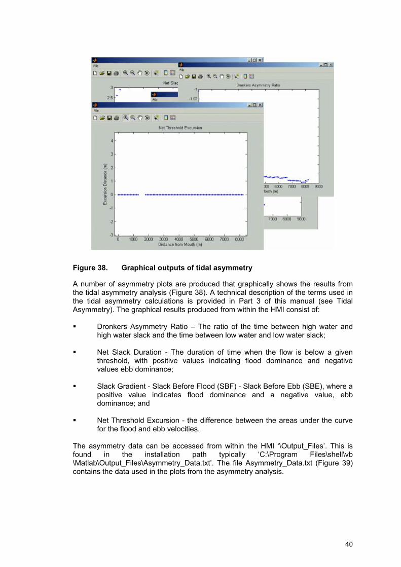
Figure 38. Graphical outputs of tidal asymmetry

A number of asymmetry plots are produced that graphically shows the results from the tidal asymmetry analysis (Figure 38). A technical description of the terms used in the tidal asymmetry calculations is provided in Part 3 of this manual (see Tidal Asymmetry). The graphical results produced from within the HMI consist of: Dronkers Asymmetry Ratio – The ratio of the time between high water and

high water slack and the time between low water and low water slack;

Net Slack Duration - The duration of time when the flow is below a given threshold, with positive values indicating flood dominance and negative values ebb dominance;

Slack Gradient - Slack Before Flood (SBF) - Slack Before Ebb (SBE), where a

positive value indicates flood dominance and a negative value, ebb dominance; and

Net Threshold Excursion - the difference between the areas under the curve

for the flood and ebb velocities. The asymmetry data can be accessed from within the HMI ‘\Output_Files’. This is found in the installation path typically ‘C:\Program Files\shell\vb \Matlab\Output_Files\Asymmetry_Data.txt’. The file Asymmetry_Data.txt (Figure 39) contains the data used in the plots from the asymmetry analysis.

40

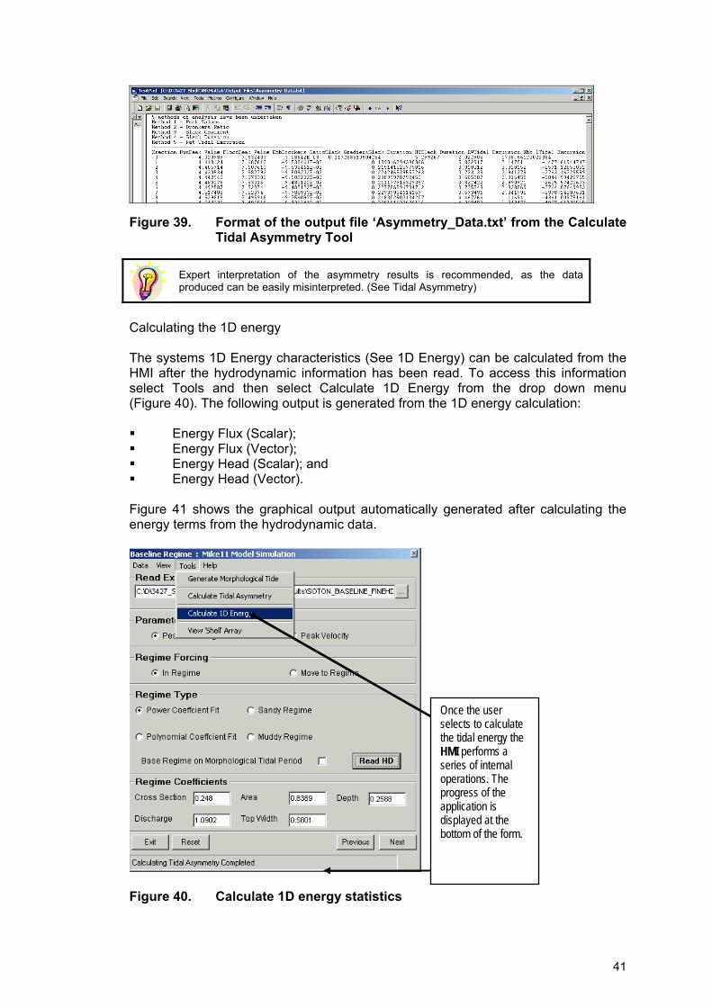
Figure 39. Format of the output file ‘Asymmetry_Data.txt’ from the Calculate

Tidal Asymmetry Tool

Expert interpretation of the asymmetry results is recommended, as the data produced can be easily misinterpreted. (See Tidal Asymmetry)

Calculating the 1D energy The systems 1D Energy characteristics (See 1D Energy) can be calculated from the HMI after the hydrodynamic information has been read. To access this information select Tools and then select Calculate 1D Energy from the drop down menu (Figure 40). The following output is generated from the 1D energy calculation: Energy Flux (Scalar); Energy Flux (Vector); Energy Head (Scalar); and Energy Head (Vector).

Figure 41 shows the graphical output automatically generated after calculating the energy terms from the hydrodynamic data.

Once the user selects to calculate the tidal energy the HMI performs a series of internal operations. The progress of the application is displayed at the bottom of the form.

Figure 40. Calculate 1D energy statistics

41

Figure 41. Graphical output from the Calculate 1D Energy analysis routine

The length of the hydrodynamic simulation should be longer than 2 tidal cycles. If the simulation length is less than this the user will not be able to proceed and the following error message will be generated (Figure 42).

Figure 42. Energy calculation warning View Shell arrays After the user has successfully read in the hydrodynamic data the HMI will create a number of internal arrays. The arrays hold the hydrodynamic and internal regime data that are used throughout the HMI. To view the internal HMI arrays select Tools – View ‘Shell’ Array (Figure 43)

42

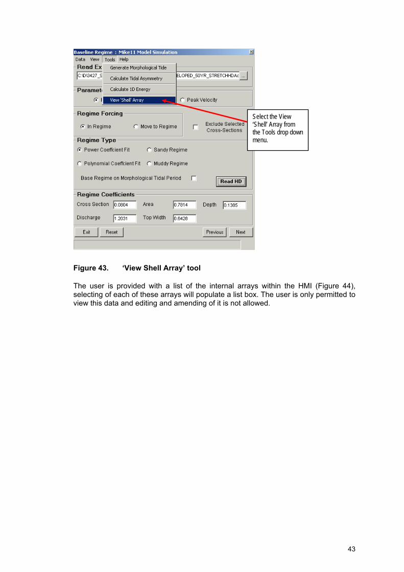
Select the View ‘Shell’ Array from the Tools drop down menu.

Figure 43. ‘View Shell Array’ tool The user is provided with a list of the internal arrays within the HMI (Figure 44), selecting of each of these arrays will populate a list box. The user is only permitted to view this data and editing and amending of it is not allowed.

43

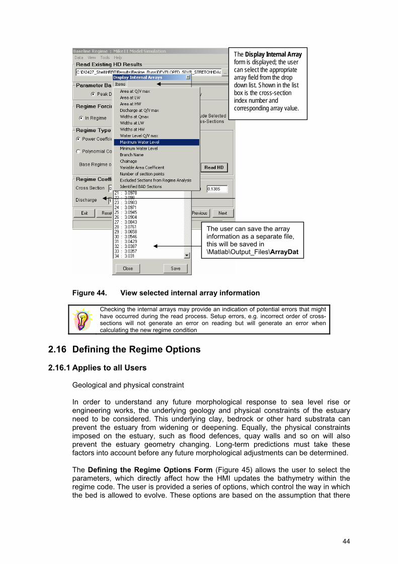
The Display Internal Array form is displayed; the user can select the appropriate array field from the drop down list. Shown in the list box is the cross-section index number and corresponding array value.

The user can save the array information as a separate file, this will be saved in \Matlab\Output_Files\ArrayDat

Figure 44. View selected internal array information

Checking the internal arrays may provide an indication of potential errors that might have occurred during the read process. Setup errors, e.g. incorrect order of cross-sections will not generate an error on reading but will generate an error when calculating the new regime condition

2.16 Defining the Regime Options

2.16.1 Applies to all Users

Geological and physical constraint In order to understand any future morphological response to sea level rise or engineering works, the underlying geology and physical constraints of the estuary need to be considered. This underlying clay, bedrock or other hard substrata can prevent the estuary from widening or deepening. Equally, the physical constraints imposed on the estuary, such as flood defences, quay walls and so on will also prevent the estuary geometry changing. Long-term predictions must take these factors into account before any future morphological adjustments can be determined. The Defining the Regime Options Form (Figure 45) allows the user to select the parameters, which directly affect how the HMI updates the bathymetry within the regime code. The user is provided a series of options, which control the way in which the bed is allowed to evolve. These options are based on the assumption that there

44

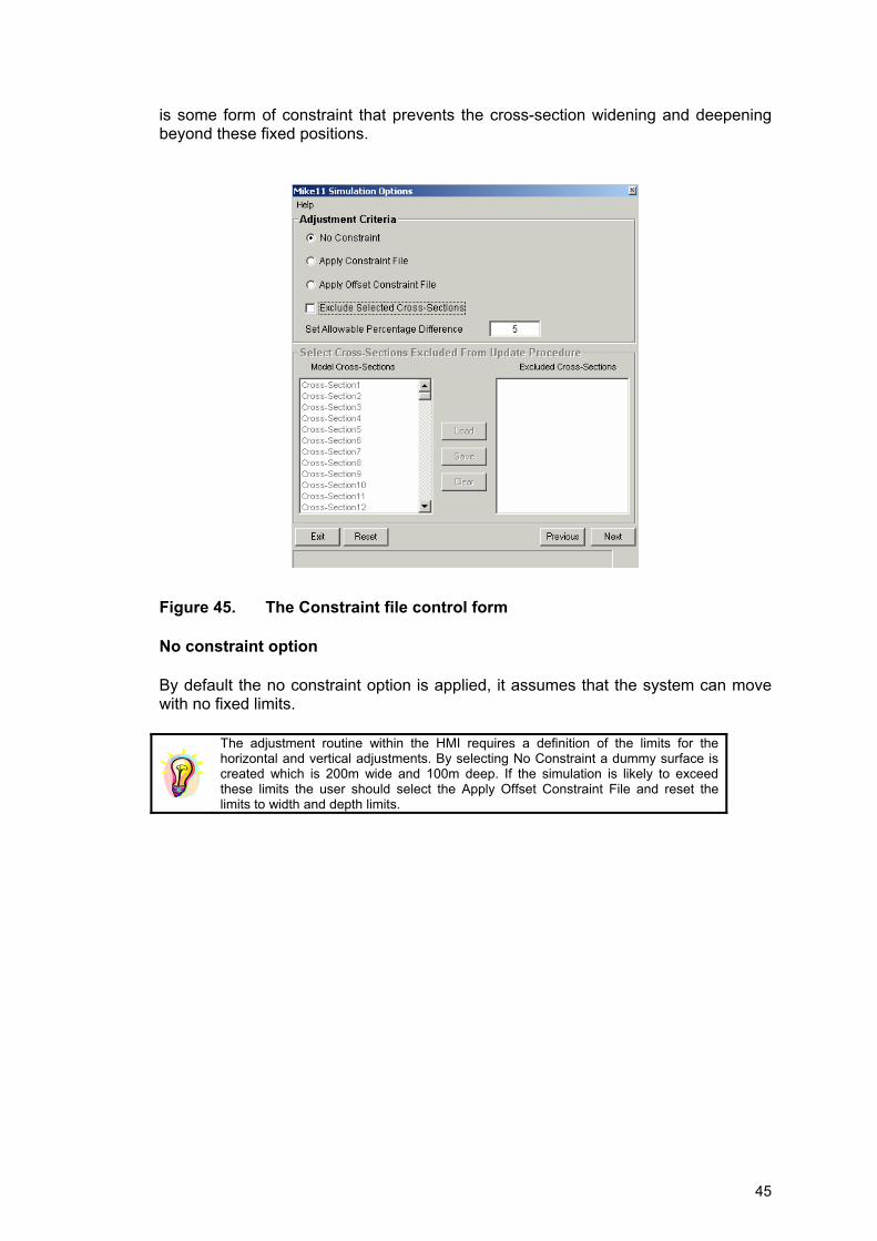
is some form of constraint that prevents the cross-section widening and deepening beyond these fixed positions.

Figure 45. The Constraint file control form No constraint option By default the no constraint option is applied, it assumes that the system can move with no fixed limits.

The adjustment routine within the HMI requires a definition of the limits for the horizontal and vertical adjustments. By selecting No Constraint a dummy surface is created which is 200m wide and 100m deep. If the simulation is likely to exceed these limits the user should select the Apply Offset Constraint File and reset the limits to width and depth limits.

45

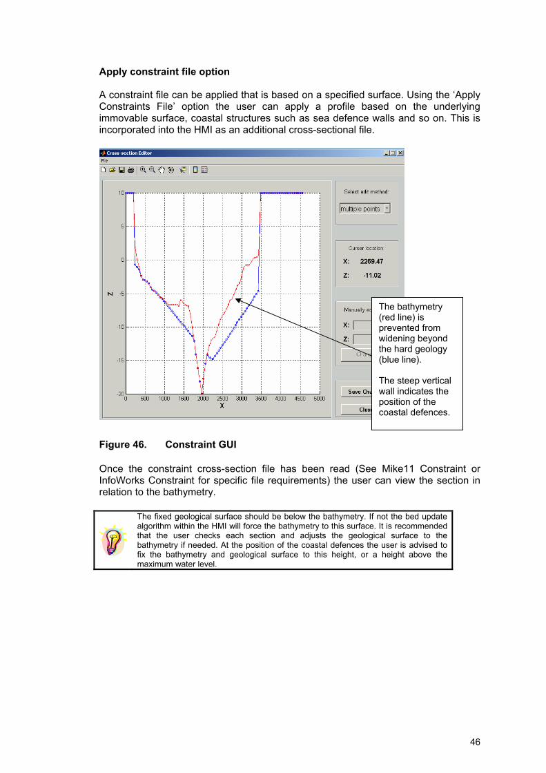
Apply constraint file option A constraint file can be applied that is based on a specified surface. Using the ‘Apply Constraints File’ option the user can apply a profile based on the underlying immovable surface, coastal structures such as sea defence walls and so on. This is incorporated into the HMI as an additional cross-sectional file.

The bathymetry (red line) is prevented from widening beyond the hard geology (blue line). The steep vertical wall indicates the position of the coastal defences.

Figure 46. Constraint GUI Once the constraint cross-section file has been read (See Mike11 Constraint or InfoWorks Constraint for specific file requirements) the user can view the section in relation to the bathymetry.

The fixed geological surface should be below the bathymetry. If not the bed update algorithm within the HMI will force the bathymetry to this surface. It is recommended that the user checks each section and adjusts the geological surface to the bathymetry if needed. At the position of the coastal defences the user is advised to fix the bathymetry and geological surface to this height, or a height above the maximum water level.

46

View/amend constraint Using the GUI (Figure 47) the user can amend the constraint file. To aid this, the corresponding bathymetry is shown allowing the user to edit the constrained section. The user can amend either single or multiple points along the constrained cross-section.

Figure 47. Amend cross-section constraint using constraint GUI

It is recommended that the user check all sections before proceeding. Errors in the HMI arise because the constrained surface has not been described correctly.

47

Apply offset constraint option By selecting the Apply Offset Constraint (Figure 48) a dummy surface is created which be default is 200m wide and 100m deep. The user is allowed to specify the vertical and horizontal limits; these determine the maximum extent to which the cross-section is allowed to expand.

The width and depth offset is based on the existing bathymetry. A 200m offset assumes a distance of 100m landward at each point fixed at the mid point along each cross-section.

Figure 48. Apply constraint offset Exclude selected cross-sections The user can choose to exclude cross-sections from the update procedure. By selecting the Exclude Selected Cross-Sections option (Figure 49), the user is able to specify the cross-sections that will be excluded from any morphological update. The excluded cross-sections are still used in the hydrodynamic simulation but are not adjusted in the update routine. To exclude defined cross-sections the user should select Exclude Selected Cross-Sections. By clicking into the check box, the lower frame within the form becomes active. Using the scroll bars the user can select sections from the Model Cross-Sections by double clicking on them. The selected cross-section will appear in the Excluded Cross-Sections list.

Typically, sections at the upstream boundary do not quickly conform to a regime state. It may be more efficient to exclude the upstream cross-sections but this depends on the particular study area.

48

Exclude selected cross-sections by checking the ‘Exclude Selected Cross-Sections’ box

Selecting the Exclude Selected Cross-Sections option enables the user to select excluded cross-sections using these menu controls

Figure 49. Select excluded cross-sections from morphological update Load excluded sections A pre-defined series of cross-sections can be excluded from the update procedure. By clicking on the Load button (Figure 49) a dialog box will appear. Select the excluded cross-section text file (how to set this up is described below) and the selected cross-sections will appear in the Excluded Cross-Sections list box. The file should be in the following format (Figure 50) with no headings or text. The numbers listing in the file represent the cross-section sequence and not the name or other ID for the cross-section. The numbers entered must be greater than 0 and less than or equal to the total number of cross-sections in the model simulation. Note as mentioned previously, within the HMI all arrays start at 0, therefore, cross-section 1 is equal to array index position 0.

2 10 20 21

Figure 50. Example of excluded cross-section import file Save excluded sections The Save button (Figure 49) allows the user to save the excluded cross-sections to file. A dialog box will appear and the user is asked to provide the location and name for this output file.

49

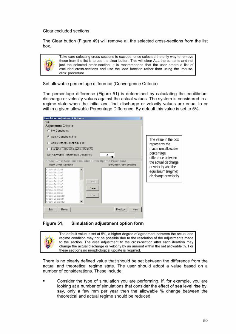
Clear excluded sections The Clear button (Figure 49) will remove all the selected cross-sections from the list box.

Take care selecting cross-sections to exclude, once selected the only way to remove these from the list is to use the clear button. This will clear ALL the contents and not just the selected cross-section. It is recommended that the user create a list of excluded cross-sections and use the load function rather than using the ‘mouse-click’ procedure

Set allowable percentage difference (Convergence Criteria) The percentage difference (Figure 51) is determined by calculating the equilibrium discharge or velocity values against the actual values. The system is considered in a regime state when the initial and final discharge or velocity values are equal to or within a given allowable Percentage Difference. By default this value is set to 5%.

The value in the box represents the maximum allowable percentage difference between the actual discharge or velocity and the equilibrium (regime) discharge or velocity

Figure 51. Simulation adjustment option form

The default value is set at 5%, a higher degree of agreement between the actual and regime condition may not be possible due to the resolution of the adjustments made to the section. The area adjustment to the cross-section after each iteration may change the actual discharge or velocity by an amount within the set allowable %. For these sections no morphological update is required.

There is no clearly defined value that should be set between the difference from the actual and theoretical regime state. The user should adopt a value based on a number of considerations. These include: Consider the type of simulation you are performing. If, for example, you are

looking at a number of simulations that consider the effect of sea level rise by, say, only a few mm per year then the allowable % change between the theoretical and actual regime should be reduced.

50

Equally, for example, large changes in mean sea level applied to the hydrodynamic boundary condition will result in a far higher degree of change between the theoretical and actual regime state. Therefore, the user may be advised to use a higher allowable % difference value.

Sensitivity tests should be undertaken to determine the importance of the

percentage difference criteria. Ultimately, this will determine the values selected/applied by the user.

Constraints – setup procedure If possible, the number of points along each constraint section should be identical to the number of points in the bathymetry cross-section i.e. if Section 1 has three bathymetry points therefore, Section 1 in the constraint file should also have three points that describe the underlying surface. The constrained section geometry orientation MUST be consistent with that of the bathymetry cross-section. By using digital terrain/geometry maps (Figure 52) of the immovable surface and extracting the elevations at known points along the cross-section this output can be easily converted to a chainage for Mike11 or added directly into InfoWorks as x,y,z values.

Generating a constraint file that has the same number of section points and the correct orientation in relation to the bathymetry cross-sections can be easily achieved in a GIS environment.

2.16.2 Mike11 Users Only

For the Mike11 simulation the user is asked to select an. xns11 file that represents the system constraints (Figure 47). The number of cross-sections in the constraint file MUST be identical to the number of cross-sections in the model simulation. The constraint cross-section file should also contain an identical number of points for each cross-section. The constrained section geometry MUST fall along the same line and orientation as the corresponding bathymetry cross-section (i.e. Zero chainage for each of the constraints and the bathymetry cross-section files should be on the same bank).

51

Figure 52. A DEM (Digital Terrain Model) of the Holocene surface for the

Humber Estuary

Figure 53. Read Geological Constraint form

By selecting the View/Amend Constraint a GUI is displayed showing the constraint and corresponding bathymetry (Figure 47). The user can choose either to reset or close the GUI but is not given the option to proceed. Closing the form will return the user to the Regime Options form.

52

The advantage of viewing the Holocene surface superimposed onto the bathymetry (Figure 47) is that it gives the user the ability to see if the Holocene is above the existing bathymetry level. This may happen due to poor resolution of the Holocene data or the timescales involved between collecting the Holocene and bathymetry datasets

2.16.3 InfoWorks Users Only

Figure 54. Read constraint file using InfoWorks

Select the text file with the cross-sections representing the immovable surface.

An InfoWorks constraint file is loaded from a comma delimited ASCII text file, the structure of the file is shown in Figure 55. Each cross-section must start with the keyword SECTION preceded by the cross-section number. As with a bathymetry file the Holocene data is then loaded as comma delimited x,y,z values.

Section 0 12333.11,133333.01,10 12500.11,133773.01,-3 Direction of file 12833.11,134231.01,10 Section 1

Figure 55. Example structure of InfoWorks constraint file The program will read the ASCII text file and make an internal check to ensure that the correct number of cross-sections have been read.

53

Figure 56. Constraint selection form for ISIS

By selecting the View/Amend Constraint a GUI is displayed showing the constraint and corresponding bathymetry. The user can either reset or close the form but is not given the option to proceed, closing the form will return the user to the regime options form.

2.17 Running a Regime Simulation

2.17.1 Applies to all Users To run a regime simulation the user is asked to select a text file that contains a single or multiple simulations.

Click here to select the simulation text file

54

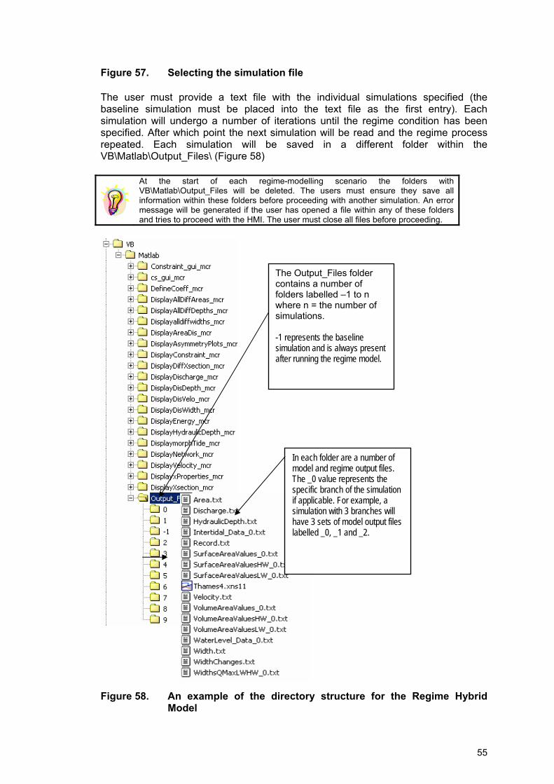
Figure 57. Selecting the simulation file The user must provide a text file with the individual simulations specified (the baseline simulation must be placed into the text file as the first entry). Each simulation will undergo a number of iterations until the regime condition has been specified. After which point the next simulation will be read and the regime process repeated. Each simulation will be saved in a different folder within the VB\Matlab\Output_Files\ (Figure 58)

At the start of each regime-modelling scenario the folders with VB\Matlab\Output_Files will be deleted. The users must ensure they save all information within these folders before proceeding with another simulation. An error message will be generated if the user has opened a file within any of these folders and tries to proceed with the HMI. The user must close all files before proceeding.

The Output_Files folder contains a number of folders labelled –1 to n where n = the number of simulations. -1 represents the baseline simulation and is always present after running the regime model.

In each folder are a number of model and regime output files. The _0 value represents the specific branch of the simulation if applicable. For example, a simulation with 3 branches will have 3 sets of model output files labelled _0, _1 and _2.

Figure 58. An example of the directory structure for the Regime Hybrid

Model

55

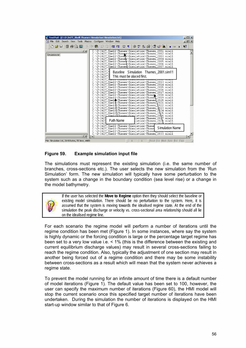
Baseline Simulation Thames_2001.sim11 This must be placed first.

Simulation Name

Path Name

Figure 59. Example simulation input file

The simulations must represent the existing simulation (i.e. the same number of branches, cross-sections etc.). The user selects the new simulation from the ‘Run Simulation’ form. The new simulation will typically have some perturbation to the system such as a change in the boundary condition (sea level rise) or a change in the model bathymetry.

If the user has selected the Move to Regime option then they should select the baseline or existing model simulation. There should be no perturbation to the system. Here, it is assumed that the system is moving towards the idealised regime state. At the end of the simulation the peak discharge or velocity vs. cross-sectional area relationship should all lie on the idealised regime line.

For each scenario the regime model will perform a number of iterations until the regime condition has been met (Figure 1). In some instances, where say the system is highly dynamic or the forcing condition is large or the percentage target regime has been set to a very low value i.e. < 1% (this is the difference between the existing and current equilibrium discharge values) may result in several cross-sections failing to reach the regime condition. Also, typically the adjustment of one section may result in another being forced out of a regime condition and there may be some instability between cross-sections as a result which will mean that the system never achieves a regime state. To prevent the model running for an infinite amount of time there is a default number of model iterations (Figure 1). The default value has been set to 100, however, the user can specify the maximum number of iterations (Figure 60), the HMI model will stop the current scenario once this specified target number of iterations have been undertaken. During the simulation the number of iterations is displayed on the HMI start-up window similar to that of Figure 6.

56

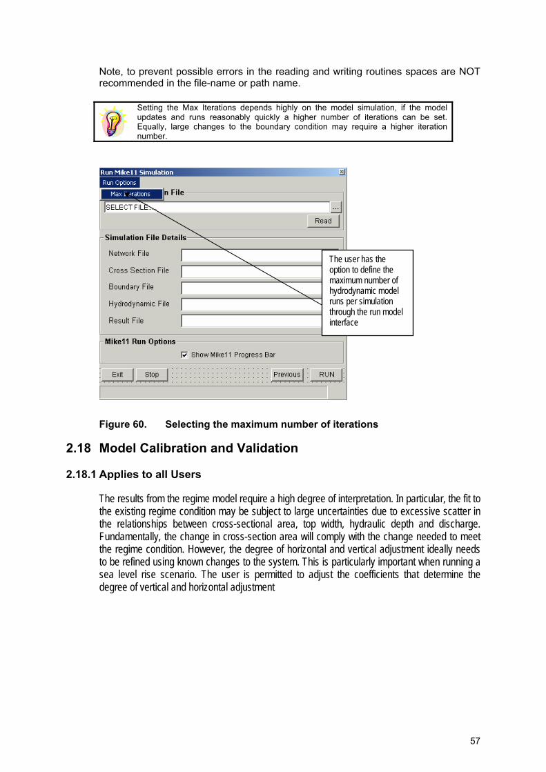
Note, to prevent possible errors in the reading and writing routines spaces are NOT recommended in the file-name or path name.

Setting the Max Iterations depends highly on the model simulation, if the model updates and runs reasonably quickly a higher number of iterations can be set. Equally, large changes to the boundary condition may require a higher iteration number.

The user has the option to define the maximum number of hydrodynamic model runs per simulation through the run model interface

Figure 60. Selecting the maximum number of iterations

2.18 Model Calibration and Validation

2.18.1 Applies to all Users The results from the regime model require a high degree of interpretation. In particular, the fit to the existing regime condition may be subject to large uncertainties due to excessive scatter in the relationships between cross-sectional area, top width, hydraulic depth and discharge. Fundamentally, the change in cross-section area will comply with the change needed to meet the regime condition. However, the degree of horizontal and vertical adjustment ideally needs to be refined using known changes to the system. This is particularly important when running a sea level rise scenario. The user is permitted to adjust the coefficients that determine the degree of vertical and horizontal adjustment

57

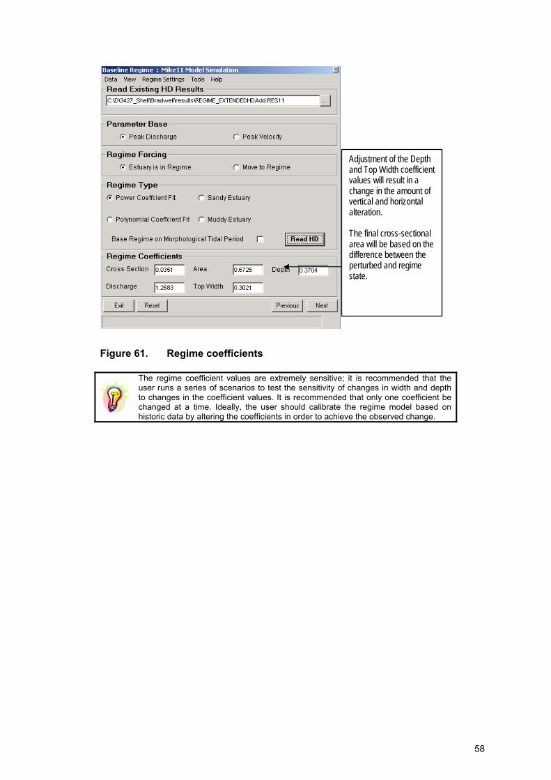
Figure 61. Regime coefficients

The regime coefficient values are extremely sensitive; it is recommended that the user runs a series of scenarios to test the sensitivity of changes in width and depth to changes in the coefficient values. It is recommended that only one coefficient be changed at a time. Ideally, the user should calibrate the regime model based on historic data by altering the coefficients in order to achieve the observed change.

Adjustment of the Depth and Top Width coefficient values will result in a change in the amount of vertical and horizontal alteration. The final cross-sectional area will be based on the difference between the perturbed and regime state.

58

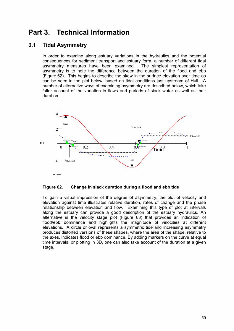
Part 3. Technical Information

3.1 Tidal Asymmetry In order to examine along estuary variations in the hydraulics and the potential consequences for sediment transport and estuary form, a number of different tidal asymmetry measures have been examined. The simplest representation of asymmetry is to note the difference between the duration of the flood and ebb (Figure 62). This begins to describe the skew in the surface elevation over time as can be seen in the plot below, based on tidal conditions just upstream of Hull. A number of alternative ways of examining asymmetry are described below, which take fuller account of the variation in flows and periods of slack water as well as their duration.

Figure 62. Change in slack duration during a flood and ebb tide To gain a visual impression of the degree of asymmetry, the plot of velocity and elevation against time illustrates relative duration, rates of change and the phase relationship between elevation and flow. Examining this type of plot at intervals along the estuary can provide a good description of the estuary hydraulics. An alternative is the velocity stage plot (Figure 63) that provides an indication of flood/ebb dominance and highlights the magnitude of velocities at different elevations. A circle or oval represents a symmetric tide and increasing asymmetry produces distorted versions of these shapes, where the area of the shape, relative to the axes, indicates flood or ebb dominance. By adding markers on the curve at equal time intervals, or plotting in 3D, one can also take account of the duration at a given stage.

0 0.2 0.4 0.6 0.8 1

4

2

2

4

tHWtLW,slack

tHW,slack

vslack

vthreshold

mTime

tLW

59

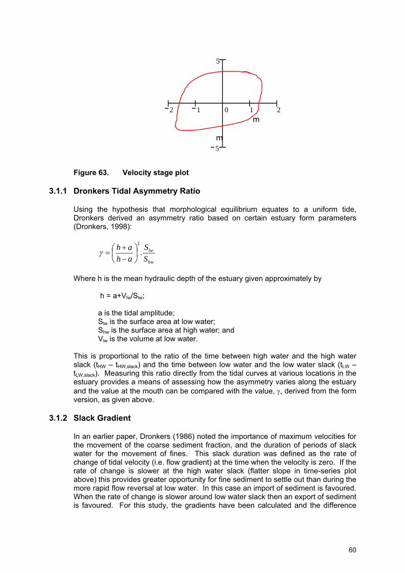
2 1 0 1 2

5

5

Figure 63. Velocity stage plot

3.1.1 Dronkers Tidal Asymmetry Ratio Using the hypothesis that morphological equilibrium equates to a uniform tide, Dronkers derived an asymmetry ratio based on certain estuary form parameters (Dronkers, 1998):

m

m

hw

lw

SS

ahah .

2

⎟⎠⎞

⎜⎝⎛

−+

=γ

Where h is the mean hydraulic depth of the estuary given approximately by

h = a+Vlw/Slw;

a is the tidal amplitude; Slw is the surface area at low water; Shw is the surface area at high water; and Vlw is the volume at low water.

This is proportional to the ratio of the time between high water and the high water slack (tHW – tHW,slack) and the time between low water and the low water slack (tLW – tLW,slack). Measuring this ratio directly from the tidal curves at various locations in the estuary provides a means of assessing how the asymmetry varies along the estuary and the value at the mouth can be compared with the value, γ, derived from the form version, as given above.

3.1.2 Slack Gradient In an earlier paper, Dronkers (1986) noted the importance of maximum velocities for the movement of the coarse sediment fraction, and the duration of periods of slack water for the movement of fines. This slack duration was defined as the rate of change of tidal velocity (i.e. flow gradient) at the time when the velocity is zero. If the rate of change is slower at the high water slack (flatter slope in time-series plot above) this provides greater opportunity for fine sediment to settle out than during the more rapid flow reversal at low water. In this case an import of sediment is favoured. When the rate of change is slower around low water slack then an export of sediment is favoured. For this study, the gradients have been calculated and the difference

60

presented (i.e. slack before flood – slack before ebb), where a positive value indicates flood dominance and a negative value ebb dominance.

3.1.3 Slack Duration Actual tidal curves can be quite complex particularly around the time of slack water. As a consequence the gradient at slack water is not always representative of the slack duration. An alternative approach is to determine the duration of time when the flow is below some threshold value, vslack. Again, taking the difference between high and low water values provides a measure of the asymmetry for the movement of fine sediments, with positive values indicating flood dominance and negative values ebb dominance.

3.1.4 Tidal Excursion Peak velocities on flood and ebb are used as a first indicator to the preferred direction of movement for the coarse sediment fraction. However, this measure takes no account of the duration of such peak velocities. It is quite common for a slightly lower velocity on one stage to prevail for much longer than the higher peak value on the opposing stage. One way to get over this is to calculate the net tidal excursion, which is simply the difference between the areas under the curve for the flood and ebb velocity. Again this may not give a wholly representative indication of movement if there are long periods at relatively low velocities. To overcome this a threshold value is introduced, vthreshold, and the area above the threshold used to calculate the respective flood and ebb excursions. Taking the difference between flood and ebb values gives the net excursion, with positive values indicating flood dominance and negative values ebb dominance.

3.2 1D Energy Terms The late fifties and early sixties saw a substantial advance in the generalisation and application of the Second Law of Thermodynamics, particularly in the context of irreversible processes (Prigogine, 1955). Leopold and Langbein (1962) applied this to the problem of river hydraulics and morphology. A subsequent paper by Langbein (1963) considered the application of the same approach to shallow estuaries. However, this deals with an 'ideal' estuary, as defined by Pillsbury (1956), and therefore is constrained by the assumption that the amplitude of the tidal elevation and velocity are constant throughout the system. The influence of the frictional terms (Lamb, 1932; Dronkers, 1986) and the interaction of M2 and M4 tidal constituents (Friedrichs and Aubury, 1988) further limit the validity of Langbein's application of this approach to the case of an estuary. In order to develop a more rigorous approach, the derivation of minimum entropy production in a river system has been re-examined. This turns out to be a special instance of the more general case of a reach with bi-directional and variable discharge. The generalised form is applied to the estuary case to investigate the relationship between morphology and tidal energy flux distribution. For the estuary case the discharge varies along its longitudinal axis within any reach. This variation of discharge will be dependent on longitudinal changes to channel depths and widths, along with the amount of water storage within a particular reach and the dissipative action of bed friction. Thus the discharge at a particular point along an estuary is dependent on the channel morphology and frictional losses. This is a fundamental distinction from the fluvial case in which discharge rates are

61

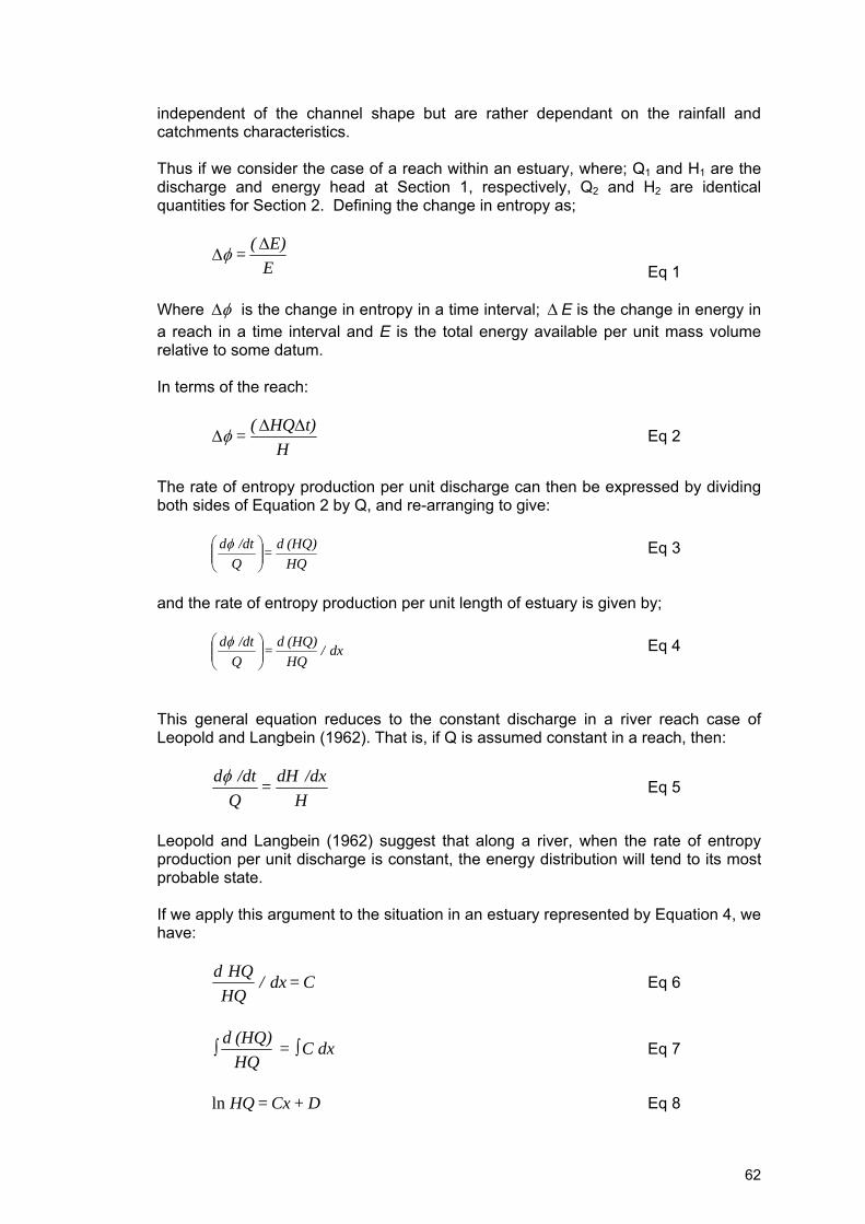
independent of the channel shape but are rather dependant on the rainfall and catchments characteristics. Thus if we consider the case of a reach within an estuary, where; Q1 and H1 are the discharge and energy head at Section 1, respectively, Q2 and H2 are identical quantities for Section 2. Defining the change in entropy as;

EE)( = Δ

Δφ

Eq 1 Where φΔ is the change in entropy in a time interval; Δ E is the change in energy in a reach in a time interval and E is the total energy available per unit mass volume relative to some datum. In terms of the reach:

Ht)HQ( = ΔΔ

Δφ Eq 2

The rate of entropy production per unit discharge can then be expressed by dividing both sides of Equation 2 by Q, and re-arranging to give:

HQ(HQ) d =

Q/dt d

⎟⎟⎠

⎞⎜⎜⎝

⎛ φ Eq 3

and the rate of entropy production per unit length of estuary is given by;

dx / HQ(HQ) d =

Q/dt d

⎟⎟⎠

⎞⎜⎜⎝

⎛ φ Eq 4

This general equation reduces to the constant discharge in a river reach case of Leopold and Langbein (1962). That is, if Q is assumed constant in a reach, then:

H/dx dH =

Q/dt dφ

Eq 5

Leopold and Langbein (1962) suggest that along a river, when the rate of entropy production per unit discharge is constant, the energy distribution will tend to its most probable state. If we apply this argument to the situation in an estuary represented by Equation 4, we have:

C = dx / HQHQ d

Eq 6

dx C = HQ(HQ) d ∫∫ Eq 7

D + Cx = HQ ln Eq 8

62

This describes the energy distribution at any given stage in the tidal cycle. Considering the complete tidal cycle we can write:

D + xC = tHQ ′′Δ∫ln Eq 9 This suggests that for the most probable distribution of energy throughout an estuary (and thus a constant production of entropy per unit discharge) the energy transferred due to the tidal wave (or conversely the work done) will decay exponentially in the upstream direction. This general model of variable discharge along a reach can incorporate energy introduced at the up stream limits of the estuary as a result of river inputs. In order to generate a solution for Equation 9, boundary conditions have to be defined in a similar manner to the fluvial case. Although it is possible to generate a tidal curve at the mouth of an estuary (as a result of harmonic theory) it is not possible to simply generate a discharge curve, the discharge curve being dependent on the morphology of the estuarine channel. However, by assuming the initial surveyed bathymetric configuration of an estuary it is possible to apply a boundary tidal curve and then generate the discharge curves via the solution of the equations of continuity of mass/volume and momentum. This may be achieved by the application of an appropriate analytical or numerical model. Having determined the boundary conditions from the numerical model, the most probable energy distribution may be determined for the applied bathymetry. This may then be compared to the actual energy distribution throughout the estuary, which may be derived from the numerical modelling results. As a result of comparing the most probable with the modelled results, areas, which are likely to experience a loss of conveyance, may be determined. Depth and width changes may then be introduced and modelled and the results compared with the updated most probable state solution. This thereby provides an iterative procedure from which the most probable state of the estuarine morphology can be determined. A further advantage of this approach is that the historical evolution of a particular estuary can be investigated (if bathymetric data is available). The analysis of historic bathymetry helps to determine whether the morphology has, historically, tended to approach or deviate away from the most probable state (alternatively the actual position may oscillate about this position through time). Such relationships provide an insight into morphological trends, help highlight any changes to the historical development and aid in determining the likely influence of anthropogenic activities (e.g. dredging, land reclamation, training wall construction) on the state of an estuary relative to the most probable state.

3.3 Morphological Tide A morphological tide has been created to reduce the computation time of a simulation by reducing the length of the water level time-series at the open boundary. This tidal period most accurately reconstructs the sediment transport results form the spring-neap tidal cycle when run for the same number as tides as that within the spring-neap tidal cycle. This tide must lead to the same flood and ebb residuals and gross transport. The use of schematised open-boundary conditions, which are considered representative in terms of their cumulative morphological effect, is based on the concept of “morphological” or “representative” boundary conditions.

63

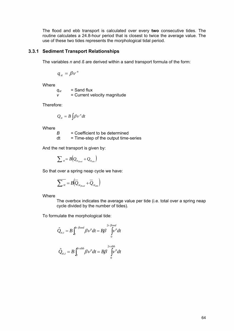
The flood and ebb transport is calculated over every two consecutive tides. The routine calculates a 24.8-hour period that is closest to twice the average value. The use of these two tides represents the morphological tidal period.

3.3.1 Sediment Transport Relationships The variables n and ß are derived within a sand transport formula of the form:

nstq βν=

Where

qst = Sand flux v = Current velocity magnitude

Therefore:

∫= dtBQ nst βν

Where B = Coefficient to be determined dt = Time-step of the output time-series And the net transport is given by:

( )∑ +=ebbflood ststst QQB

So that over a spring neap cycle we have:

( )ebbflood ststst QQB +=∑

Where

The overbox indicates the average value per tide (i.e. total over a spring neap cycle divided by the number of tides).

To formulate the morphological tide:

∫∫×

×==

floodnflood n

tst dtBdtBQ2

0

2

0,ˆ νββν

∫∫×

×==

ebbnebb n

tst dtBdtBQ2

0

2

0,ˆ νββν

64

On a given time-series, the average over the spring neap cycle is given by:

( )

28

.28

0tve

fQ

nT

Δ+=∑ ν

( )

28

.28

0tve

eQ

nT

Δ−=∑ ν

∑ −= eQfQst For i = 1…28

( )

2

.ˆ

2

,

∑+

Δ+=

Ti

i

t

t

n

fi

tveQ

ν

( )

2

.ˆ

2

,

∑+

Δ−=

Ti

i

t

t

n

ei

tveQ

ν

∑ −= eifisti QQ ,,,ˆˆ

( ) ( ) ( )∑ ∑−+−+−= ststieeiffii QQQQR ,,,

ˆˆ The minimum value of R indicates the ith tide that is the closest match to the estimated transport regime

( )

28

.0

∑=

Δ+=

Non

i

n

f

tveQ

ν

Where

tΔ = the hydrodynamic output time-step; N = number of data points in spring neap cycle

Define start points for each tide (spring neap cycle) ( )iN :

( )

2ˆ

2

,

∑+

Δ×+=

Ni

Ni

n

fi

tveQ

ν

65

A second morphological tide could also be developed to account for the presence of waves. Typically, this tide may have smaller amplitudes than that of the morphological tide developed for tide alone conditions. To produce a more accurate simulation two morphological tides will be applied one in the tide alone case and one in the wave and tide case.

3.4 Bed Updating Routine

3.4.1 Applies to all Users The bed update method used is essentially that presented by Dennis et al (2000) and works by adjusting the width and depth of the cross-section based on how far away from the idealised regime state the section lies. If the discharge or velocity through the cross-section is greater or less than the idealised state then typically the section area will be adjusted to meet the regime state. The update routines work firstly by obtaining the values of maximum discharge or velocity at points along the estuary, along with the accompanying cross-sectional areas of flow. The regime equation is written a Qe = aQb where: Qe = Discharge equilibrium a, b = Constants in the relationship Establish constants in an assumed exponential variation of cross-sectional area AQ and width TQ with peak discharge Qmax or velocity. The constants (a, b) are again obtained from fitting to the results of the initial model run.

66

y = 2.085x - 11.147

2

3

4

5

6

7

8

9

10

11

12

7 7.5 8 8.5 9 9.5 10 10.5

Log (Area)

Log

(Dis

char

ge)

Figure 64. Parametric fit of the log (area) to the log (discharge)

In this example the exponent p = 2.085.

y = 2.704x - 12.31

2

3

4

5

6

7

8

9

10

11

12

7 7.2 7.4 7.6 7.8 8 8.2 8.4

Log (Top Width)

Log

(Dis

char

ge)

Figure 65. Parametric fit of the log (top width) to the log (discharge) In this example the exponent q = 2.704.

67

y = 3.6216x + 2.4915

0

2

4

6

8

10

12

0 0.5 1 1.5 2 2

Log (Mean Hydraulic Depth)

Log

(Dis

char

ge)

.5

Figure 66. Parametric fit of the log (hydraulic depth) to the log (discharge) In this example the exponent r = 3.6216.

After calculating the regime fits (Figure 66), the bathymetry for each cross-section is altered after each iteration until it satisfies the regime relationship within a specified level of tolerance. The peak discharge at each cross-section is compared to the one predicted by the regime relationship and the latter is divided by the former to give a value, σ, for each cross-section i. The value σ constitutes a measure of closeness of the ith cross-section to an equilibrium state. A value greater than one indicates that accretion will occur, while a value less than one indicates erosion. The cross-section width and then depth is adjusted so that the actual discharge or velocity would approach that of the equilibrium discharge/velocity. The width of the channel at all points is multiplied by a width factor σp. Similarly, the elevation of all points in the cross-section under the depth of maximum discharge is raised or lowered by the depth factor σq.

Factor Width σp = p

nn QQBB ⎟⎟

⎠

⎞⎜⎜⎝

⎛=+

max1 ; and

Factor Depth σq = q

nn QQHH ⎟⎟

⎠

⎞⎜⎜⎝

⎛=+

max1

The process of adjustment is carried out for all cross-sections and is subject to a tolerance process. Typically, cross-sections that have a small cross-sectional area may be unstable, therefore, large changes in cross-sectional area may mean that they never reach an equilibrium condition. The tolerance factor prevents the full adjustment to the section from occurring. This reduction in the amount of change that can occur to a cross-section may potentially reduce the total number of iterations required to meet the required estuary equilibrium.

68

Typically, a tolerance factor of 90% is applied after 5 iterations. After 11 iterations this dampening factor increases to 98%. The cross-sections are allowed to evolve beyond the maximum high water line; this is designed to prevent unrealistic profiles. In particular, protruding land at the margins of the cross-section. The adjustment of the land behind the high-water line will play no part in the hydrodynamic calculations, although in reality this would not occur. The adjustment routine calculates the position of the adjusted point in relation to some fixed (Holocene) surface. If the position of the new point lies beyond this the routine places the point at the same elevation as the fixed surface. Updating steps 1) Extract Qmax and the simultaneous cross-sectional area at each cross-section

location along the estuary.

2) At each section, test to see if the current discharge and the equilibrium discharge are within a specified level of accuracy. If the regime criterion is satisfied, then the cross-section will not require updating. Otherwise, update the cross-section by applying factor width and depth:

3) The details of updating the cross-section are as follows:

Apply factor width first to update the section top width B: Tn+1 = Tn(Qn+1/Qregime)p, where Qregime is calculated using the cross-

sectional area of flow derived from the 1D model run at the current iteration step. This change in the cross-section is applied to the horizontal positions of the (x, z) section coordinates.

Apply a factor depth to change the bed elevations so that the cross-section also satisfies the regime requirements:

An+1 = An(Qn+1/Qregime), where Qregime is calculated using the cross-

sectional area of flow derived from the 1D model run at the current iteration step.

4) A test is performed to see if the new z(i) position lies above or below the

physical constraint. Note, if the user applies no constraint a dummy constraint is set some 100m below the existing bathymetry. If the point lies below the constrained surface then this z(i) point is fixed to the same elevation as this constraint.

5) The 1D model is run with the updated cross-sections and this process is

repeated until a convergence to within the specified % difference has been obtained throughout the model domain.

The default convergence accuracy of 5% is that adopted by Dennis et al. In the Humber study for Emphasys, a convergence level of 1% was applied. Typically, a value of 5% is applied to provide results in a efficient time frame, It is recommended that the user adjust this parameter in order to asses the sensitivity of the specific system.

69

3.5 Proposed Approach The existing approach as described within the HMI manual, does not consider the physical aspects of the hydrodynamics within the morphological bed updating routine. This is to say (excluding the influence of constraints) the bed updating approach changes all of the depths across the cross-section profile by the same proportional amount (i.e. all depths change by the same percentage). However, different parts of the channel cross-sections vary in the way they respond to larger (or smaller) discharges and the response of different cross-sections will vary from each. In order to address this issue an internal workshop was held in January 2007 at HR Wallingford, one suggested approach to providing a more realistic representation of morphological change in the model is described below.

3.5.1 Hypsometry Method Let each cross-section be defined by a number of (distance, elevation) points (xi ,zi ). The depth of each point below a reference water level is denoted as hi .

rii hKh .=Δ

Where Δhi is the predicted change in depth at the I.th measurement of elevation at an estuary transect. r > 1 implies more of a change in the deeper depths while r < 1 implies that there is less of a (proportional) change in depth in the deepest parts of the channel than in the shallower parts. It is necessary to derive the formula for r in terms of the discharge or velocity along the estuary. This formula is assumed to be valid throughout the evolution of the estuary after some disturbance. The formula is based on the idea that a small change to a cross-section must essentially preserve the cross-section shape and therefore the value of r at any cross-section must be a function of the initial cross-section shape. By analysing each cross-section shape we can derive a set of values of r which (using a regime assumption) can be associated with the maximum discharge or velocity through each of the sections to give a formula r=f(Q). Derivation of r=f(Q) For each transect: Either,

( ) ( )22

11 −+ +−

+=Δ iiii

ixxxx

x

Calculate the "width” associated with each ( )ii hx , point in the transect. Sort the measurements of depth and transect distance so that the various measurements of depth are ranked lowest to highest. Calculate a new set of transect distances

∑Δ=′ jj xx where j is the jth ranked data point.

70

You get a set of values of x’ (j), h (j) where j is the position of the measurement in the ranking. Fit the best fitting "power law" curve to the set of values x’ (j), h (j) [where h (j) is the "y" value and x’ (j) the "x" value] i.e. h (i)=K.x'(i) r , r is then the exponent of the power law best fit. Or, Interpolate the measurements of depth onto depths that are EVENLY SPACED across the transect. Rank the various measurements of depth (to whatever level) of the estuary bathymetry according to lowest to highest. You get a set of values of h(i) where i is the position of the measurement in the ranking. Fit the best fitting "power law" curve to the set of values [i,h(i)] where h(i) is the "y" value and i the "x" value i.e. h(i)=K.i r . r is then the exponent of the power law best fit (a rectangular channel would give r is zero, a triangular channel would give r is 1) Then, You then have a set of values for r and a known discharge Q or Velocity V that is associated with this value r(Q) is then whatever is the best fit (some reasonable function) of the data points [Q,r].

Use of r during prediction of evolution During the evolution of the estuary the regime algorithms will, on each iteration, predict a certain change in cross-section area at each cross-section. Also, since the discharge through the cross-section is known the value of r can also be determined. This change in area is equal to i

riii xhKxhA Δ=ΔΔ=Δ ∑∑ ..

This equation can be solved to find K and then find for each point in the transect. Note K will have to be recalculated for each section for each iteration.

rii hKh .=Δ

The following can summarize the proposed approach:

Work out the depths h (i) below the level of maximum discharge or velocity; Sort the values of x (i) and h (i) so that the values of h (i) are in ascending

order; If the values of x (i) are not evenly spaced then the values of (x (i+1)-x (i-1))/2

will also have to be sorted along with x and h; Plot the ascending values of h against i (where i is the ith depth) for evenly

spaced depths or plot the ascending levels of h against the sum of (x (j+1)-x (j 1))/2 for j=1,I;

r is found from a best fit plot of h(i) against i or h(i) against x(i) - it will be the exponent of the power law (Figure 67).

71

Figure 67. Cross-section sorted by depth, power fit (red line) is shown

through the data set Applicability of the method Note, in cross-section profiles that have a significant proportion of intertidal flat (Figure 68) then the proposed method has some limitations. Fitting a power law through the depth sorted cross-section profile (Figure 69) produces a much poorer R2 value (here we use R to denote the Pearson correlation coefficient to avoid confusion with r ) than a linear fit, indicating that the original method (which assumes r =1) is a better model in this instance. Thus in general it is suggested that that the fit of the power law method be compared to the fit using a linear relationship and the best model used as the basis for establishing the value of r. An alternative methodology would be to divide the cross-section into the morphological components e.g. flats and the channel, and work out values of r for each (Figure 70). It is recognised that in general it would be beneficial to characterise the effect of a change in flow at each point in the cross-section, thus improving the model further but further development of this nature was outside the scope of the work identified for this project.

72

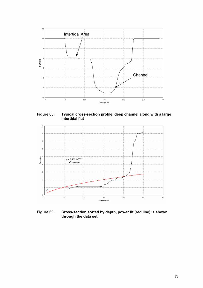
Figure 68. Typical cross-section profile, deep channel along with a large intertidal flat

Intertidal Area

Channel

Figure 69. Cross-section sorted by depth, power fit (red line) is shown through the data set

73

Figure 70. Cross-section sorted by depth, 2 power fits (red line and blue) are shown with the cross-section profile being divided into inter and sub-tidal zones

3.6 Constraint File

3.6.1 Applies to all Users

In order to prevent the adjustment of the cross-section exceeding a fixed width and/or depth a geological constraint can be applied. The cross-section must still be allowed to reduce its area (top width and depth). A geological constraint may represent a quay wall, rocky outcrop, hard substrata (i.e. Rock) and so on. It is extremely unlikely that under such conditions the corresponding parts/all of that section would increase in depth and width (Figure 71)

74

Figure 71. Examples of geologically restricted cross-sections

Geologically Restricted Section

Numbering direction of cross-section points.

n

Required Widening

k

x

Ne Ns

Ns

Geologically Restricted Section

Numbering direction of cross-section points.

n Required Widening

k

x

Ne

X1

Geologically Restricted Section

Numbering direction of cross-section points.

Geologically Restricted Section

75

3.7 Estimate of Estuary Water Volume

3.7.1 Applies to all Users The calculation of the wet area within each of the cross-sections is performed in the module AreaCalc. The AreaCalc routine calculates the area of the cross-section under a specific water level at a particular state of the tide (peak discharge, velocity, high or low water) using the following concept:

( ) ( )( ) ( ) ( )( )∑−

⎟⎠⎞

⎜⎝⎛ −−×

++=

inichainageichainageiareaiareaVolume 1

21

Where i = the cross-section number; and chainage(i) = the distance between each cross-section.

The area of the cross-section below i.e. peak discharge water level is calculated by a mid-ordinate rule method using a trapezoidal approach, where the x, z bathymetric co-ordinates were used to mark out the successive trapeziums as shown in (Figure 72). For trapeziums crossing the specified water level, (x, z) co-ordinates were linearly interpolated.

The calculation of the volumes enables testing of the model by comparison with actual observed values. Volume calculations provide a method to predict the change in estuary capacity as a result of a change in forcing condition e.g. predicted sea level rise.

(Modified after: Barker, 1999)

Figure 72. The method used in the 1D hybrid model for the calculation of the cross-sectional areas and intertidal width

The HMI also provides a measure of the intertidal areas within the estuary at various water level conditions. Crossing points are identified that specify the position along the cross-section where the water level intersects. These sections are then added together to provide an estimate of the intertidal width. The advantage of this

76

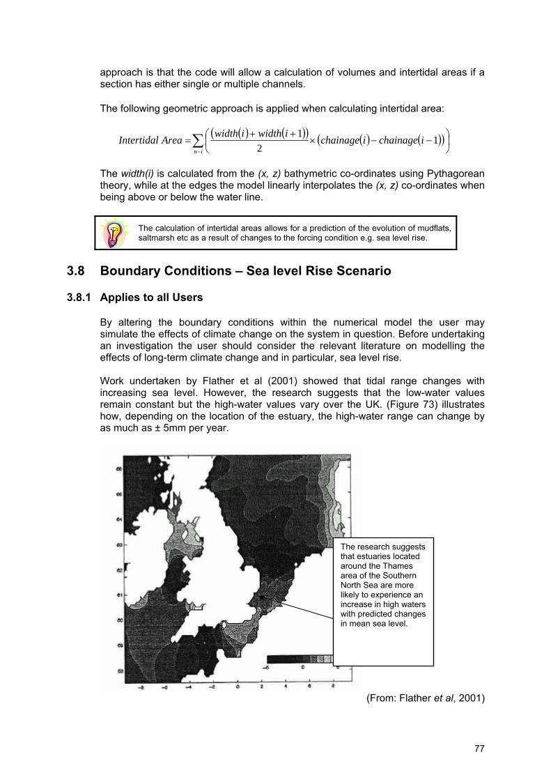
approach is that the code will allow a calculation of volumes and intertidal areas if a section has either single or multiple channels. The following geometric approach is applied when calculating intertidal area:

( ) ( )( ) ( ) ( )( )∑−

⎟⎠⎞

⎜⎝⎛ −−×

++=

inichainageichainageiwidthiwidthAreaIntertidal 1

21

The width(i) is calculated from the (x, z) bathymetric co-ordinates using Pythagorean theory, while at the edges the model linearly interpolates the (x, z) co-ordinates when being above or below the water line.

The calculation of intertidal areas allows for a prediction of the evolution of mudflats, saltmarsh etc as a result of changes to the forcing condition e.g. sea level rise.

3.8 Boundary Conditions – Sea level Rise Scenario

3.8.1 Applies to all Users

By altering the boundary conditions within the numerical model the user may simulate the effects of climate change on the system in question. Before undertaking an investigation the user should consider the relevant literature on modelling the effects of long-term climate change and in particular, sea level rise. Work undertaken by Flather et al (2001) showed that tidal range changes with increasing sea level. However, the research suggests that the low-water values remain constant but the high-water values vary over the UK. (Figure 73) illustrates how, depending on the location of the estuary, the high-water range can change by as much as ± 5mm per year.

(From: Flather et al, 2001)

The research suggests that estuaries located around the Thames area of the Southern North Sea are more likely to experience an increase in high waters with predicted changes in mean sea level.

77

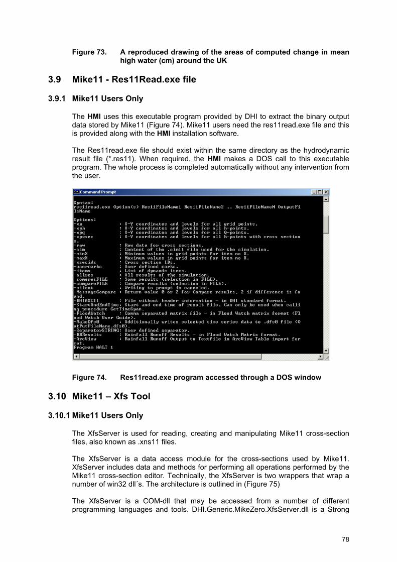
Figure 73. A reproduced drawing of the areas of computed change in mean high water (cm) around the UK

3.9 Mike11 - Res11Read.exe file

3.9.1 Mike11 Users Only

The HMI uses this executable program provided by DHI to extract the binary output data stored by Mike11 (Figure 74). Mike11 users need the res11read.exe file and this is provided along with the HMI installation software. The Res11read.exe file should exist within the same directory as the hydrodynamic result file (*.res11). When required, the HMI makes a DOS call to this executable program. The whole process is completed automatically without any intervention from the user.

Figure 74. Res11read.exe program accessed through a DOS window 3.10 Mike11 – Xfs Tool

3.10.1 Mike11 Users Only

The XfsServer is used for reading, creating and manipulating Mike11 cross-section files, also known as .xns11 files. The XfsServer is a data access module for the cross-sections used by Mike11. XfsServer includes data and methods for performing all operations performed by the Mike11 cross-section editor. Technically, the XfsServer is two wrappers that wrap a number of win32 dll´s. The architecture is outlined in (Figure 75) The XfsServer is a COM-dll that may be accessed from a number of different programming languages and tools. DHI.Generic.MikeZero.XfsServer.dll is a Strong

78

named .NET assembly that may be used from C#, managed C++, Visual Basic .NET and other .NET compliant languages.

Figure 75. XfsServer overall architecture

3.11 InfoWorks RS.com Tools

3.11.1 InfoWorks Users Only InfoWorks is based on operating the ISIS hydrodynamic model through the InfoWorks RA model interface. The InfoWorks RS.com files allows this connection to be performed in a dynamic environment. For a more simplistic approach of how this coupling has been achieved please see the example contained within the folder INFOWORKS_Example.

DHI Generic MikeZero XfsServer.dll (NET assembly)

XfsServer.dll (Com dll)

Ufs.dll

mzlanguage.dll

libxm2.dll pfs2004.dll

ams2004.dll

3.12 Shell Interface Code

An example of the Visual Basic 6 and Matlab code is shown below (Figure 76). In the Visual Basic code the black text is the executable code, the green text is the non-executable description. Code highlighted in red has a compiler error and should be corrected. The descriptive text (green) is provide throughout the Visual basic code and can be used as a guide to show the user the meaning of each element within the interface software. The Matlab code (Figure 77) has been written as individual scripts and compiled to executable files that can be called from within the visual basic environment. The Matlab code has been designed to read a number of external result files produced from within the HMI. As with the Visual Basic code the areas highlighted in green are non-executable.

79

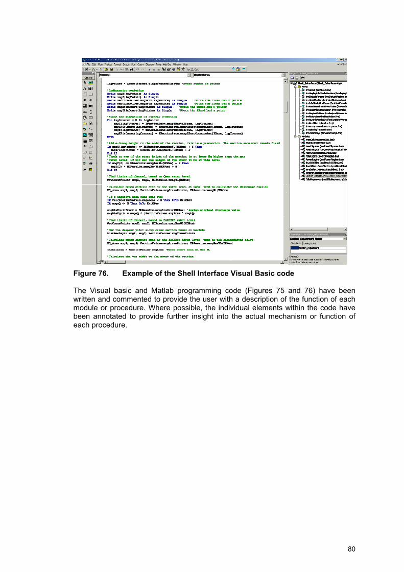
Figure 76. Example of the Shell Interface Visual Basic code The Visual basic and Matlab programming code (Figures 75 and 76) have been written and commented to provide the user with a description of the function of each module or procedure. Where possible, the individual elements within the code have been annotated to provide further insight into the actual mechanism or function of each procedure.

80

Figure 77. Example of the Matlab (*.m) code

81

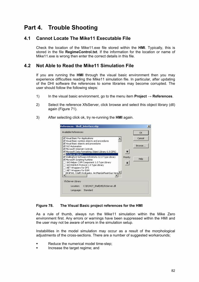
Part 4. Trouble Shooting

4.1 Cannot Locate The Mike11 Executable File Check the location of the Mike11.exe file stored within the HMI. Typically, this is stored in the file RegimeControl.txt. If the information for the location or name of Mike11.exe is wrong then enter the correct details in this file.

4.2 Not Able to Read the Mike11 Simulation File If you are running the HMI through the visual basic environment then you may experience difficulties reading the Mike11 simulation file. In particular, after updating of the DHI software the references to some libraries may become corrupted. The user should follow the following steps: 1) In the visual basic environment, go to the menu item Project → References. 2) Select the reference XfsServer, click browse and select this object library (dll)

again (Figure 71). 3) After selecting click ok, try re-running the HMI again.

Figure 78. The Visual Basic project references for the HMI As a rule of thumb, always run the Mike11 simulation within the Mike Zero environment first. Any errors or warnings have been suppressed within the HMI and the user may not be aware of errors in the simulation setup. Instabilities in the model simulation may occur as a result of the morphological adjustments of the cross-sections. There are a number of suggested workarounds; Reduce the numerical model time-step; Increase the target regime; and

82

Increase the numerical dampening within the code. Within the Section_Adjustment module is a routine that suppresses the amount of change based on the iteration number. The following lines of code showe the tolerance routine.

If RegimeControls.mintSimulationNum < 5 Then ‘Less than 5 iterations RegimeControls.msngDamping = 1 ‘No tolerance Else If RegimeControls.mintSimulationNum > 5 And _RegimeControls.mintSimulationNum < 11 Then ‘Between 5 and 11 iterations RegimeControls.msngDamping = 0.1 ‘90% tolerance Else ‘After 11 iterations RegimeControls.msngDamping = 0.02 ‘98% tolerance End If

If the error occurs at only one particular section, it may be possible to exclude

that section from the update routine. For example, sections upstream may become unstable if a high discharge has been applied. Use the ‘Exclude Sections’ option to exclude them from the simulation.

Errors within the Asymmetry and Energy calculation routines are typically a result of a section drying or the simulation length being too short to calculate the energy within the system. A number of routines have been added to try and capture these occurrences but the user should ensure they check that all sections have some flow during the simulation. The model takes a long time to reach equilibrium? To try and reduce the number of iterations required to reach an equilibrium state the user should try the following: Increase the number of points around the zone of minimum and maximum

water within each cross-section (Figure 79)

Increase the ‘Maximum Allowable % Difference’. This is the value between the existing and equilibrium maximum discharge/velocity through the cross-section.

Switch off those sections that might be causing a problem. Typically, sections

upstream have been shown to cause instabilities in the regime update procedure. often the cross-sections that lie upstream lie on the lower end of the discharge vs. area plot. Therefore, greater changes occur at these sections than at sections that lie on the upper part of the discharge vs. area relationship plot.

If running a sea level rise scenario, the user can try and run the scenario

based on a smaller number of sea level rise (slr) adjustments applied at the water level boundary of the hydrodynamic model. e.g: 100-year Sea Level Rise Scenario = 6mm*100 = 60cm increase in msl.

83

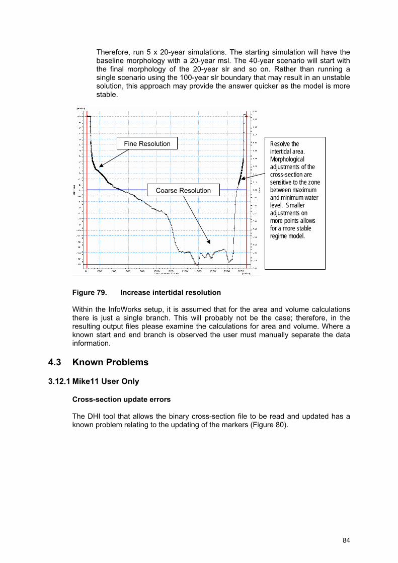
Therefore, run 5 x 20-year simulations. The starting simulation will have the baseline morphology with a 20-year msl. The 40-year scenario will start with the final morphology of the 20-year slr and so on. Rather than running a single scenario using the 100-year slr boundary that may result in an unstable solution, this approach may provide the answer quicker as the model is more stable.

Figure 79. Increase intertidal resolution

Resolve the intertidal area. Morphological adjustments of the cross-section are sensitive to the zone between maximum and minimum water level. Smaller adjustments on more points allows for a more stable regime model.

Fine Resolution

Coarse Resolution

Within the InfoWorks setup, it is assumed that for the area and volume calculations there is just a single branch. This will probably not be the case; therefore, in the resulting output files please examine the calculations for area and volume. Where a known start and end branch is observed the user must manually separate the data information.

4.3 Known Problems

3.12.1 Mike11 User Only Cross-section update errors The DHI tool that allows the binary cross-section file to be read and updated has a known problem relating to the updating of the markers (Figure 80).

84

The point highlighted by the red box has NOT been identified as the lowest point along the section (defined as a red circle).

Figure 80. A typical Mike11 cross-section profile after a morphological update

The incorrect positioning of the cross-section markers should be taken into account by the user if used to define the area of flow within the cross-section. Typically, the markers are used as a reference for the displaying of the cross-section. However, in those instances where the user has defined a series of user defined markers then this known error should be taken into account.

85

Part 5. References ABP Research, 1999. Historic analysis of Humber morphology, Humber Estuary Geomorphology Studies - Stage 2, Binnie, Black & Veatch for the Environment Agency, ABP Research & Consultancy Ltd, Research Report No: R.839. ABPmer, 2003. Historical analysis of Humber estuary morphology, Report for Environment Agency, North East Region, ABP Marine Environmental Research Ltd, Report No: R.1005, 1-16. ABPmer 2005. Severn Estuary CHaMP Morphological Assessments Part A: Regime Modelling. ABP Marine Environmental Research Ltd. Report No. R.1260a Dennis JM, Spearman JR, Dearnaley MP, 2000, The development of a regime model for prediction of the long-term effects of civil engineering activities on estuaries, Phys. Chem. Earth (B), 25(1), 45-50. Dronkers J, 1986, Tidal asymmetry and estuarine morphology, Netherlands Journal of Sea Research, 20, 117-131 Flather, R.A., Baker, T.F., Woodworth, P.L., Vassie, J.M. and Blackman, D.L. 2001. Integrated effects of climate change on coastal extreme sea levels. Proceedings of the 36th DEFRA Conference of River and Coastal Engineers. 03.4.1 – 03.4.12 Friedrichs CT and Aubrey DG, 1988, Non-linear tidal distortion in shallow well-mixed estuaries: a synthesis, Estuarine Coastal and Shelf Science, 27, 521-546 Lamb H, 1932, Hydrodynamics, Cambridge University Press Langbein WB, 1963, The hydraulic geometry of a shallow estuary, Bulletin of Int Assoc Sci Hydrology, 8, 84-94. Leopold LB and Langbein WB, 1962, The concept of entropy in landscape evolution, Geological Survey Professional Paper, 500-A, A1-A20 O’Connor B.A. Nichols, J. Rayner R, 1990, Estuary Geometry as a function of Tidal Range In: 22nd International Conference of Coastal Engineering, American Society of Civil Engineers, 3 (Chapter 231), pp. 3050-3062. [7] Newson, M. D. and Sear, D. A., 1994. Sediment and gravel transportation in Rivers, National River Authority, R and D Note C5/384/2, Bristol. Norton PA, Manning AJ, Townend IH, Lane A, Karunarathna G. Application and Inter-comparison of Estuary Morphological Models. Paper 03-5, 42nd Defra Flood and Coast Management Conference. Pillsbury GB, 1956, Tidal Hydraulics, Vicksburg, Mississippi, Corps of Engineers, U S Army Price, D and Norton, P. 2000. Emphasis Consortium Phase 1B – Modelling Results. MAFF Report, Contract CSA 4938, Project FD1401. [8]

86

Prigogine I, 1955, Introduction to thermodynamics of irreversible processes, London, John Wiley & Son Wright, A.P. & Townend, I.H. 2006. Predicting Intertidal Change in Estuaries. 41st Defra Flood and Coastal Management Conference.

87