ship roll motion reduction by means of the...
TRANSCRIPT

Michele Macovez
Ship Roll Motion Reduction by Means of the Rudder Master’s thesis, march 2008

Ship Roll Motion Reduction by Means of the Rudder
The report has been prepared by: Michele Macovez Supervisor: Mogens Blanke
DTU Electrical Engineering Automation Technical University of Denmark Elektrovej Building 326 DK-2800 Kgs. Lyngby Denmark www.elektro.dtu.dk/English/research/au.aspx Tel: (+45) 45 25 35 50 Fax: (+45) 45 88 12 95
Date of publishing:
19-03-2008
Classification:
Public
Comments:
This report is submitted in partial fulfilment of the requirements for the Master degree at the Technical University of Denmark. The report represents 35 ECTS point.
Copyright:
© Michele Macovez, 2008

AbstractThis thesis focuses on the design of rudder roll stabilization (RRS) systems.
Some results of the research to solve this speci�c ship motion control problem arepresented. The modelling of the ship dynamics are discussed in the �rst chapters:both the non linear model and the linear one have been obtained. Since the ship'sroll motion is caused by waves, a wave model is de�ned, assuming the disturbanceas a stochastic process.
Two different feedback control approaches are analyzed and implemented.The �rst method aims at �nding a control law that minimizes the variance of theoutput. The second approach directly shapes the output sensitivity function, whichrelates the wave disturbance to the ship roll motion, to achieve good disturbancerejection. The non minimum phase dynamics in the rudder-to-roll response resultsin some fundamental limitations in control system design. A trade-off betweendisturbance attenuation at some frequencies and ampli�cation at others affects theperformances of the feedback controllers.
Results of sea-way simulations show that both these controllers have goodperformances. The maximum roll damping is greater than 55% for both the ana-lyzed controllers. The best roll reduction has been obtained by the minimum vari-ance cheap controller with a damping of almost 70%.
iii

AcknowledgmentsI would like to thank my supervisor, ProfessorMogens Blanke for his patience
in teaching me so many things and for his guidance during the period of my thesis.I thank Ph.D. Roberto Galeazzi for his availability and support.
Special appreciation go to my Italian supervisor Professor Thomas Parisinifor allowing me to come to Denmark to work on this project.
I would like to thank my parents for always being there and giving me thepossibility to spend these months in Copenhagen, my brother Roberto and Michela.Tender thanks go to Sara for her understanding and for staying by me.
iv

Table of contents
Table of contents . . . . . . . . . . . . . . . . . . . . . . . . . . . . . . . . . . . . . . . . . . . . . . . . . . . . . . . . . . . . . . . . v
List of Figures . . . . . . . . . . . . . . . . . . . . . . . . . . . . . . . . . . . . . . . . . . . . . . . . . . . . . . . . . . . . . . . . viii
List of Tables . . . . . . . . . . . . . . . . . . . . . . . . . . . . . . . . . . . . . . . . . . . . . . . . . . . . . . . . . . . . . . . . . . . xi
Introduction . . . . . . . . . . . . . . . . . . . . . . . . . . . . . . . . . . . . . . . . . . . . . . . . . . . . . . . . . . . . . . . . . . . . . 1
Motivations . . . . . . . . . . . . . . . . . . . . . . . . . . . . . . . . . . . . . . . . . . . . . . . . . . . . . . . . . . . . . . . . . . . . . . 2
Relevant Literature . . . . . . . . . . . . . . . . . . . . . . . . . . . . . . . . . . . . . . . . . . . . . . . . . . . . . . . . . . . . . . . 2
Problem statement . . . . . . . . . . . . . . . . . . . . . . . . . . . . . . . . . . . . . . . . . . . . . . . . . . . . . . . . . . . . . . . . 3
Objectives . . . . . . . . . . . . . . . . . . . . . . . . . . . . . . . . . . . . . . . . . . . . . . . . . . . . . . . . . . . . . . . . . . . . . . . 4
Main results of the Thesis . . . . . . . . . . . . . . . . . . . . . . . . . . . . . . . . . . . . . . . . . . . . . . . . . . . . . . . . . 4
Thesis Outline . . . . . . . . . . . . . . . . . . . . . . . . . . . . . . . . . . . . . . . . . . . . . . . . . . . . . . . . . . . . . . . . . . . . 5
1 Ship dynamics . . . . . . . . . . . . . . . . . . . . . . . . . . . . . . . . . . . . . . . . . . . . . . . . . . . . . . . . . . . . . . . . 7
1.1 Equations of Motion . . . . . . . . . . . . . . . . . . . . . . . . . . . . . . . . . . . . . . . . . . . . . . . . . . . . . . . . . 8
1.2 Forces and Moments acting on a ship . . . . . . . . . . . . . . . . . . . . . . . . . . . . . . . . . . . . . . . . 12
1.3 Control Devices . . . . . . . . . . . . . . . . . . . . . . . . . . . . . . . . . . . . . . . . . . . . . . . . . . . . . . . . . . . . 14
1.3.1 Forces acting on the rudder . . . . . . . . . . . . . . . . . . . . . . . . . . . . . . . . . . . . . . . . . . 14
1.3.2 Rudder-Propeller Interaction . . . . . . . . . . . . . . . . . . . . . . . . . . . . . . . . . . . . . . . . . 16
2 Simulation Model . . . . . . . . . . . . . . . . . . . . . . . . . . . . . . . . . . . . . . . . . . . . . . . . . . . . . . . . . . 18
v

Table of contents vi
2.1 Nonlinear State-Space Model . . . . . . . . . . . . . . . . . . . . . . . . . . . . . . . . . . . . . . . . . . . . . . . 18
2.2 Multi-Role naval vessel simulator . . . . . . . . . . . . . . . . . . . . . . . . . . . . . . . . . . . . . . . . . . . 19
2.2.1 Rudder machinery . . . . . . . . . . . . . . . . . . . . . . . . . . . . . . . . . . . . . . . . . . . . . . . . . . . 19
2.2.2 Rudder . . . . . . . . . . . . . . . . . . . . . . . . . . . . . . . . . . . . . . . . . . . . . . . . . . . . . . . . . . . . . . 20
2.2.3 Naval vessel . . . . . . . . . . . . . . . . . . . . . . . . . . . . . . . . . . . . . . . . . . . . . . . . . . . . . . . . . 20
2.3 System Linearization . . . . . . . . . . . . . . . . . . . . . . . . . . . . . . . . . . . . . . . . . . . . . . . . . . . . . . . 22
2.3.1 Rudder to Roll transfer function . . . . . . . . . . . . . . . . . . . . . . . . . . . . . . . . . . . . . . 24
2.3.2 Non-minimum Behavior in Ship Response . . . . . . . . . . . . . . . . . . . . . . . . . . . . 25
3 Environmental Disturbances . . . . . . . . . . . . . . . . . . . . . . . . . . . . . . . . . . . . . . . . . . . . . 28
3.1 Wind generated waves . . . . . . . . . . . . . . . . . . . . . . . . . . . . . . . . . . . . . . . . . . . . . . . . . . . . . . 28
3.2 Stochastic representation . . . . . . . . . . . . . . . . . . . . . . . . . . . . . . . . . . . . . . . . . . . . . . . . . . . 29
3.3 Nonlinear models of wave spectra . . . . . . . . . . . . . . . . . . . . . . . . . . . . . . . . . . . . . . . . . . . 30
3.4 Linear approximations of wave spectra . . . . . . . . . . . . . . . . . . . . . . . . . . . . . . . . . . . . . . 31
3.5 Encounter frequency. . . . . . . . . . . . . . . . . . . . . . . . . . . . . . . . . . . . . . . . . . . . . . . . . . . . . . . . 33
3.6 Waves simulation model . . . . . . . . . . . . . . . . . . . . . . . . . . . . . . . . . . . . . . . . . . . . . . . . . . . . 34
4 Ship Roll Stabilization . . . . . . . . . . . . . . . . . . . . . . . . . . . . . . . . . . . . . . . . . . . . . . . . . . . . . 36
4.1 Stabilizing Methods . . . . . . . . . . . . . . . . . . . . . . . . . . . . . . . . . . . . . . . . . . . . . . . . . . . . . . . . 36
4.2 Rudder Roll Damping Control Systems . . . . . . . . . . . . . . . . . . . . . . . . . . . . . . . . . . . . . . 39
4.3 Sensitivity function . . . . . . . . . . . . . . . . . . . . . . . . . . . . . . . . . . . . . . . . . . . . . . . . . . . . . . . . . 40
4.4 Ship motion performance . . . . . . . . . . . . . . . . . . . . . . . . . . . . . . . . . . . . . . . . . . . . . . . . . . . 41
4.4.1 Reduction of Roll at Resonance-RRR. . . . . . . . . . . . . . . . . . . . . . . . . . . . . . . . . 41
4.4.2 Reduction of Statistics of Roll -RSR . . . . . . . . . . . . . . . . . . . . . . . . . . . . . . . . . . 42
4.4.3 Reduction of Probability of Roll Peak Occurrence -RRO . . . . . . . . . . . . . . 42

Table of contents vii
5 Cheap limiting optimal control . . . . . . . . . . . . . . . . . . . . . . . . . . . . . . . . . . . . . . . . . . . 44
5.1 Minimum Variance Cheap Control . . . . . . . . . . . . . . . . . . . . . . . . . . . . . . . . . . . . . . . . . . 44
5.2 Stability and Performance Trade-offs . . . . . . . . . . . . . . . . . . . . . . . . . . . . . . . . . . . . . . . . 49
5.2.1 Output variance . . . . . . . . . . . . . . . . . . . . . . . . . . . . . . . . . . . . . . . . . . . . . . . . . . . . . 51
5.3 Numerical simulations and results . . . . . . . . . . . . . . . . . . . . . . . . . . . . . . . . . . . . . . . . . . . 52
5.4 Cheap controller robustness . . . . . . . . . . . . . . . . . . . . . . . . . . . . . . . . . . . . . . . . . . . . . . . . . 58
6 Sensitivity function-based approach control . . . . . . . . . . . . . . . . . . . . . . . . . . . . 62
6.1 Single notch sensitivity speci�cation . . . . . . . . . . . . . . . . . . . . . . . . . . . . . . . . . . . . . . . . 62
6.2 Numerical simulations and results . . . . . . . . . . . . . . . . . . . . . . . . . . . . . . . . . . . . . . . . . . . 65
6.3 Double notch sensitivity speci�cation . . . . . . . . . . . . . . . . . . . . . . . . . . . . . . . . . . . . . . . 71
6.4 Numerical simulations and results . . . . . . . . . . . . . . . . . . . . . . . . . . . . . . . . . . . . . . . . . . . 73
6.5 Sensitivity based approach controller robustness . . . . . . . . . . . . . . . . . . . . . . . . . . . . . 79
7 Conclusions . . . . . . . . . . . . . . . . . . . . . . . . . . . . . . . . . . . . . . . . . . . . . . . . . . . . . . . . . . . . . . . . . 83
7.1 Future work . . . . . . . . . . . . . . . . . . . . . . . . . . . . . . . . . . . . . . . . . . . . . . . . . . . . . . . . . . . . . . . . 84
References . . . . . . . . . . . . . . . . . . . . . . . . . . . . . . . . . . . . . . . . . . . . . . . . . . . . . . . . . . . . . . . . . . . . . 85
A Naval vessel data . . . . . . . . . . . . . . . . . . . . . . . . . . . . . . . . . . . . . . . . . . . . . . . . . . . . . . . . . . . 88
A.1 Principal multipurpose naval vessel data . . . . . . . . . . . . . . . . . . . . . . . . . . . . . . . . . . . . . 88
A.2 Manoevering coef�cients . . . . . . . . . . . . . . . . . . . . . . . . . . . . . . . . . . . . . . . . . . . . . . . . . . . 89

List of Figures
1.1 Ship motion components. . . . . . . . . . . . . . . . . . . . . . . . . . . . . . . . . . . . . . . . . . . . 7
1.2 Geometrical aspects of the rudder. . . . . . . . . . . . . . . . . . . . . . . . . . . . . . . . . . . . 15
1.3 Lift and Drag on the rudder. . . . . . . . . . . . . . . . . . . . . . . . . . . . . . . . . . . . . . . . . 15
1.4 Rudder-Propeller interaction. . . . . . . . . . . . . . . . . . . . . . . . . . . . . . . . . . . . . . . . 17
2.1 Block diagram of the system. . . . . . . . . . . . . . . . . . . . . . . . . . . . . . . . . . . . . . . . 19
2.2 Rudder machinery. . . . . . . . . . . . . . . . . . . . . . . . . . . . . . . . . . . . . . . . . . . . . . . . . 20
2.3 Frequency characteristic of the open loop transfer functions. . . . . . . . . . . . . . . . 23
2.4 Poles and zeros of the rudder to roll transfer function. . . . . . . . . . . . . . . . . . . . . 25
2.5 Non-minimum-phase effect on roll dynmamics during a turn to port. . . . . . . . . 26
3.1 Power spectrum of the linear approximation and thePierson-Moskovitz model. . . . . . . . . . . . . . . . . . . . . . . . . . . . . . . . . . . . . . . . . . . 32
3.2 Incident sea description and denomination for sailing conditions. . . . . . . . . . . . 33
3.3 Encounter frequency versus actual frequency. . . . . . . . . . . . . . . . . . . . . . . . . . . 34
3.4 Simulink block diagram for wave disturbances. . . . . . . . . . . . . . . . . . . . . . . . . . 35
3.5 Wave disturbance simulation . . . . . . . . . . . . . . . . . . . . . . . . . . . . . . . . . . . . . . . . 35
4.1 Examples of U-tube tanks. . . . . . . . . . . . . . . . . . . . . . . . . . . . . . . . . . . . . . . . . . . 37
4.2 Fin stabilizer arrangement. . . . . . . . . . . . . . . . . . . . . . . . . . . . . . . . . . . . . . . . . . 38
4.3 Rudder roll stabilization (RRS) system structure . . . . . . . . . . . . . . . . . . . . . . . . 40
viii

List of Figures ix
4.4 Rayleigh probability density function . . . . . . . . . . . . . . . . . . . . . . . . . . . . . . . . . 43
5.1 Bode plot of wave disturbance �lter H(s) . . . . . . . . . . . . . . . . . . . . . . . . . . . . . . 46
5.2 Sensitivity function for the proper and improper cheap controller. . . . . . . . . . . . 48
5.3 Nyquist plots of L(j!) for the unstable and stable plant. . . . . . . . . . . . . . . . . . . 49
5.4 Cheap controller sensitivity function varying the ratio between Tand T1. . . . . . . . . . . . . . . . . . . . . . . . . . . . . . . . . . . . . . . . . . . . . . . . . . . . . . . . . . 50
5.5 Ratio between the output variance and the white noise variance fordifferent frequencies. . . . . . . . . . . . . . . . . . . . . . . . . . . . . . . . . . . . . . . . . . . . . . . 52
5.6 Cheap controller system sensitivity function. . . . . . . . . . . . . . . . . . . . . . . . . . . . 53
5.7 Simulation at Bow seas with wave period of 6 seconds. . . . . . . . . . . . . . . . . . . . 55
5.8 Simulation at Beam seas with wave period of 8 seconds. . . . . . . . . . . . . . . . . . . 56
5.9 Simulation at Head seas with wave period of 10 seconds. . . . . . . . . . . . . . . . . . 57
5.10 Cheap controller roll reduction ratio as function of wave period. . . . . . . . . . . . . 58
5.11 Cheap controller roll reduction ratio as function of wave periodvarying the ship speed. . . . . . . . . . . . . . . . . . . . . . . . . . . . . . . . . . . . . . . . . . . . . 59
5.12 Cheap controller roll reduction ratio as function of wave period.Variation in roll damping coef�cient. . . . . . . . . . . . . . . . . . . . . . . . . . . . . . . . . . 60
5.13 Cheap controller roll reduction ratio as function of wave periodvarying the wave disturbance. . . . . . . . . . . . . . . . . . . . . . . . . . . . . . . . . . . . . . . . 61
6.1 Bode plot of the single notch sensitivity speci�cation. . . . . . . . . . . . . . . . . . . . . 63
6.2 Bode plot of ~G' (s) : . . . . . . . . . . . . . . . . . . . . . . . . . . . . . . . . . . . . . . . . . . . . . . 64
6.3 Bode plot of the output sensitivity function for the single notchspeci�cation. . . . . . . . . . . . . . . . . . . . . . . . . . . . . . . . . . . . . . . . . . . . . . . . . . . . . 66

List of Figures x
6.4 Simulation at Head seas with wave period of 8 seconds. . . . . . . . . . . . . . . . . . . 68
6.5 Simulation at Beam seas with wave period of 6 seconds. . . . . . . . . . . . . . . . . . . 69
6.6 Simulation at Bow seas with wave period of 10 seconds. . . . . . . . . . . . . . . . . . . 70
6.7 Single notch sensitivity based approach roll reduction ratio asfunction of wave period. . . . . . . . . . . . . . . . . . . . . . . . . . . . . . . . . . . . . . . . . . . . 71
6.8 Double notch sensitivity speci�cation. . . . . . . . . . . . . . . . . . . . . . . . . . . . . . . . . 72
6.9 Bode plot of the output sensitivity function for the double notchspeci�cation. . . . . . . . . . . . . . . . . . . . . . . . . . . . . . . . . . . . . . . . . . . . . . . . . . . . . 74
6.10 Simulation at Quartering seas with wave period of 8 seconds. . . . . . . . . . . . . . . 76
6.11 Simulation at Beam seas with wave period of 10 seconds. . . . . . . . . . . . . . . . . . 77
6.12 Simulation at Head seas with wave period of 6 seconds. . . . . . . . . . . . . . . . . . . 78
6.13 Double notch sensitivity based approach roll reduction ratio asfunction of wave period. . . . . . . . . . . . . . . . . . . . . . . . . . . . . . . . . . . . . . . . . . . . 79
6.14 Sensitivity based approach controller roll reduction ratio varyingthe ship speed. . . . . . . . . . . . . . . . . . . . . . . . . . . . . . . . . . . . . . . . . . . . . . . . . . . . 80
6.15 Sensitivity based approach controller roll reduction ratio varyingthe roll damping coef�cient . . . . . . . . . . . . . . . . . . . . . . . . . . . . . . . . . . . . . . . . . 80
6.16 Sensitivity based approach controller roll reduction ratio varying �. . . . . . . . . . 81

List of Tables
1.1 Generalized displacements of a vessel . . . . . . . . . . . . . . . . . . . . . . . . . . . . . . . . . 8
2.1 Rudder data adopted for the multi role naval vessel . . . . . . . . . . . . . . . . . . . . . . 20
2.2 Principal dimensions of multi role naval vessel . . . . . . . . . . . . . . . . . . . . . . . . . 21
5.1 Cheap controller performances for a 6 seconds period wave disturbance . . . . . . 53
5.2 Cheap controller performances for a 8 seconds period wave disturbance . . . . . . 54
5.3 Cheap controller performances for a 10 seconds period wavedisturbance . . . . . . . . . . . . . . . . . . . . . . . . . . . . . . . . . . . . . . . . . . . . . . . . . . . . . . 54
6.1 Single notch sensitivity approach controller performances for a 6seconds period wave disturbance . . . . . . . . . . . . . . . . . . . . . . . . . . . . . . . . . . . . . 67
6.2 Single notch sensitivity approach controller performances for a 8seconds period wave disturbance . . . . . . . . . . . . . . . . . . . . . . . . . . . . . . . . . . . . . 67
6.3 Single notch sensitivity approach controller performances for a 10seconds period wave disturbance . . . . . . . . . . . . . . . . . . . . . . . . . . . . . . . . . . . . . 67
6.4 Double notch sensitivity approach controller performances for a 6seconds period wave disturbance . . . . . . . . . . . . . . . . . . . . . . . . . . . . . . . . . . . . . 75
6.5 Double notch sensitivity approach controller performances for a 8seconds period wave disturbance . . . . . . . . . . . . . . . . . . . . . . . . . . . . . . . . . . . . . 75
6.6 Double notch sensitivity approach controller performances for a 10seconds period wave disturbance . . . . . . . . . . . . . . . . . . . . . . . . . . . . . . . . . . . . . 75
A.1 Main data for multipurpose naval vessel used in the project and forthe simulation. . . . . . . . . . . . . . . . . . . . . . . . . . . . . . . . . . . . . . . . . . . . . . . . . . . . 88
xi

List of Tables xii
A.2 hydrodynamic parameters for multipurpose vessel used in theproject and for the simulation. . . . . . . . . . . . . . . . . . . . . . . . . . . . . . . . . . . . . . . . 89

IntroductionThe problem of ship stabilization has widely been studied in the last decades. Perez
[22] gave a detailed overview on the main efforts done in this �eld in chapter 10 of hisbook. The idea of using the rudder as a stabilization device is quite recent and it probablyemerged from observations of ship roll behavior under autopilot operation. Taggart [26]reported one particular situation observed during a Trans Atlantic voyage of a high-speedcontainer ship in the winter of 1967. During this trip the characteristics of an autopilot con-troller were tested under different sea conditions, and it was pointed out that under certaincircumstances, the rudder induced signi�cant roll motion. Motivated by these observations,in 1972 aboard the motor yacht M.S. Peggy in The Netherlands, , van Gunsteren [30] per-formed full-scale trials using the rudder as the only stabilizing actuator. The same thing didCowley and Lambert [6] in 1972 using an autopilot and a roll feedback loop.
During the 1980s there was an interesting contribution to the issue of rudder rollstabilization (RRS) developed in different countries: The Netherlands, Denmark, Swedenand the USA. In 1983 van der Klugt [29] and van Amerongen [28] performed full scaletrials consequently the designing of a controller based on Linear Quadratic Gain (LQG)techniques but this kind of approach didn't give the results expected. Laudval and Fossen[17] proposed an improvement for such a mechanism and the performances were goodclose to the roll natural frequency but deteriorated at lower and higher frequencies. InDenmark the Royal Danish Navy introduced RRS on some of their fast monohull patrolvessels and the experiments were conducted by Blanke [4]. Different control approacheswere considered such as LQG andH1 techniques. Källström [15] in collaboration with theRoyal Swedish Navy (RSN) implemented a RRS that became later in 1987 a commercialproduct known by the name of ROLL-NIX. The system was designed for use on straightcourses; it switched off automatically when major manoeuvring was required, and backon when the vessel resumed a steady course. Baitis & Schmidt [1] presented in 1989the use of rudder roll stabilization employed by the U.S. Navy on a DD-963 (Spruance)class destroyer. The rudder roll stabilizer signal was added to the signal generated by theautopilot or by manual steering. The installed systems produced reductions in roll motionof approximately 40%.
During the 1990s, there was signi�cant research activity on the theoretical aspects ofthe problem. Several different control techniques were proposed, but only a few full-scaleimplementations were reported. Blanke and Christensen [3] studied the sensitivity of theperformance of LQ control to variations in the coupling coef�cients of the equations ofmotion. They used a linear model based on the hydrodynamic data estimated during thedesign stage of the SF300 vessels of the Danish Navy.
In Sweden Källström and Shultz [16] continued to describe the performances ofROLL-NIX and its adaptive properties while in Denmark Hearns and Blanke [13] pro-posed the use of Quantitative Feedback Theory to design cascade SISO controllers for rolland yaw. Laudval and Fossen [18] took the nonlinear approach, (maybe the only referencein the literature that uses a nonlinear model for the design) and proposed the use of slidingmode control.
1

Introduction 2
MotivationsMarine vehicles are designed to operate with acceptable reliability and economy, and inorder to accomplish this, it is essential to regulate the dynamics of the ship. The motions ofships and the control of those motions have been the focal point of extensive research overthe years. A ship in a seaway undergoes complex motions that may weaken the operationalrange of the ship and be uncomfortable and sometimes even dangerous for the crew. Incertain circumstances, the captain may be obligated to alter course or slow down the shipto reduce large motions. This could produce undesirable mission limitations for militaryvessels and reduce pro�ts for commercial vessels. Controlling the ship motion is of greatinterest to many parties in the marine �eld since motion control during station keeping orlow-speed maneuvers may broaden the safety range of many vessels.
Over the years, many types of motion control have been devised. The majority havebeen aimed at reducing roll motions since the force required to reduce roll is reasonablysmall compared to the weight of the ship. Moreover, roll is the largest and most undesirablecomponent of ship motion. Different methods and devices have been designed to reduceship roll motions. For an example, anti-roll �ns are used in cases of high ship speeds,and bilge keels, anti roll tanks, gyroscopic stabilizers have been employed to accomplisha good roll reduction. Although most of the devices work well, additional and externalpower installations will lead to the weight increase and space decrease on the ship. Thehydrodynamic stability and structural strength may be changed when for example anti-rolltanks are adopted. The installation cost is also generally raised and the ship speed may bedecreased due to additional components.
Hence the present work focuses on the use of the rudder to reduce the roll motion ofthe ship. The main reasons for this are that almost every ship has a rudder (thus no extraequipment may be necessary), and also because this technique can be used in conjunctionwith other stabilizers. Based on frequency characteristics of the rudder in�uence on yawand roll motions, the two objectives can be separated in the frequency domain. Small fre-quencies are used for heading control, while high frequencies for roll reduction. A primarymotivation of this project is also to provide a simulation environment to assess the feasibil-ity of various control strategies in various sea states without the expense of model testingduring design iterations.
Relevant LiteratureThe literature on marine control has grown in the last decades. A comprehensive treatmentof automatic control systems for marine vehicles has been given by Fossen [9]. He providedmathematical foundations and theory needed for the designing of ship control systems. Healso focused on both linear and nonlinear models to describe the dynamic and kinematicequations of motion of marine vehicles and the subject of stability and control. In his workhe explored in depth the modeling of ocean vehicles, environmental disturbances, and the

Introduction 3
sensor and navigation systems, as well as discussing in length the applications of moderncontrol theory.
A more detailed investigation on some of these aspects has then been provided byPerez [22]. A deep coverage of hydrodynamic aspects related to control, wave inducedmotion modelling and roll stabilization was furnished. He studied the particular prob-lems of control system design for course autopilots, rudder roll stabilization and combinedrudder-�n stabilizers, and the fundamental issues of performance limitations for the par-ticular problems of rudder and �n roll stabilization. He also reviewed the fundamentalperformance limitations of the closed-loop system due to the dynamic characteristics ofthe ship. A relevant work in this sector has been done by Blanke [2]. He concentrated hisresearch on rudder-roll damping (RRD) autopilots. He showed through parametric inves-tigations that cross-couplings between steering and roll might give rise to problems withperformance robustness for the RRD controller. He then treated the RRD design problemfrom a robust control outset. He demonstrated that a separation result exists that makes itpossible to make separate roll and steering speci�cations and optimize the two controllersindependently.
Recently together with Yang [33] he has worked on H1 control of the roll damp-ing loop and with Hearns [13] on qualitative feedback theory (QFT) applied to solve thecombined RRD-heading control problem with due regard of model uncertainty.
Problem statementIt is well-known that to fully represent the motion of a rigid body in space a six-degrees-of-freedom approach is required. To determine the position and orientation six independentcoordinates are necessary: the �rst three and their derivatives describe the translationalmotion of the rigid body in terms of positions and linear velocities, while the last three co-ordinates and their time derivatives identify the rotational motion in terms of orientationand angular velocities. The six different motion components are de�ned as surge (trans-lation along the x-axis), sway (translation along the y-axis), heave (translation along thez-axis), roll (rotation about the x-axis), pitch (rotation about the y-axis) and yaw (rotationabout the z-axis). However, for a control problem as roll stabilization, it is often assumedthat the ship motion can be described using only four degrees of freedom, which includesurge, sway, yaw and roll.
The equations of motion describing the dynamics of a ship are readily obtained fromNewton's law in space-�xed coordinate. However, to take advantage of the symmetryproperty of a ship, a ship-�xed coordinate system is preferred. With the origin for the axissystem taken at the center of gravity of the ship, the ship equations of motion within a �xedcoordinate system can be found.
The vessel used for the modelling corresponds to a small monohull [3]. The datahave been gathered by Blanke and Christensen at the project state and are estimated by theDanish Maritime Institute, DMI. The ship is considered to advance keeping a steady courseat a constant forward speed U .

Introduction 4
The irregularity of ocean waves gives rise to sudden and unpredictable growth of theroll amplitude. Waves with absolute frequency !0 and angle of encounter � are are includedin the model, representing the disturbance acting on the vessel. These wave disturbancesare modelled as �ltered white noise with constant power spectral density. The �lter adoptedis a second order transfer function with dominant frequency equal to !0:
It is an aim of this thesis to design a controller capable of reducing the wave rollinduced motion.
ObjectivesShip roll motion is caused by external disturbances, e.g. wave, wind and current, whichcontribute to the roll by exerting varying forces and moments on the hull. Roll motion,however, is not only caused by the action of the waves, but it can also be generated by therudder. The rudder's main function is to change the heading of a ship; however, the ruddermay also be used to produce, or correct, roll motion. An alteration of course makes theship heel and when the ship rights itself, it turns back towards its equilibrium position in adamped oscillation.
The effectiveness of RRD controls has been debated. Results from full scale evalua-tion on vessels have indicated very satisfactory results showing 50-70 % roll reduction. Bycontrast, other experiences have demonstrated much less effectiveness in certain cases. Al-though rudder roll stabilizers have been designed since the early 80's, it still represents achallenging objective. An automatic control system is necessary to provide the rudder com-mand based on the measurements of ship motion. A good model of the vessel is neededin order to reproduce the behavior of the real system. The objectives of the thesis are toderive a mathematical model of the system to be controlled and to design and implementa feedback control law to damp the roll motion generated by the waves. The performancelimitations, due to fundamental physical constraints, have to be discussed and taken in con-sideration.
Main results of the ThesisThe work that has been done during this project led to the following results:
� A mathematical model for the non linear system of the ship motion in the seaway
has been determined.

Introduction 5
� The system has been linearized around a stationary point for the task of control
design.
� The effects of the wave disturbances on ships and their stochastic representation
have been illustrated.
� A �rst controller design for the reduction of the roll motion has been implemented:
minimum variance cheap controller. The maximum damping achieved was 68%.
� A second controller design has been employed: sensitivity function based approach
controller. Two different speci�cations have been tested:
� A narrow frequency range disturbance attenuation with maximum damping of
62% was obtained.
� A wider frequency range disturbance attenuation with maximum damping of
56% was obtained.
� The robustness of the system for small changes in the ship parameters has been
assessed.
Thesis OutlineThe thesis is structured as follows:
In the �rst two Chapters the geometrical aspects of the ship and the equations whichgovern the motions of the ship in the seaway are presented. A nonlinear model is ob-tained and the simulation environment is described. A linear state space model, obtainedby linearizing the nonlinear model around a stationary point, is employed to design thecontroller.

Introduction 6
Chapter 3 introduces the environmental disturbances affecting the cruising of a ves-sel. Both linear and non linear methods to reproduce wind generated waves disturbancesare investigated. A stochastic approach is considered and the model used for the wavedisturbance is shown.
Chapter 4 provides an overview of the techniques commonly used for roll stabiliza-tion giving some general informations on each method. The model used for the RRDsystem is introduced and the �gures usually adopted to asses the motion performance ofthe ship are reviewed.
A �rst type of controller is developed in Chapter 5. It is the minimum variancecheap controller and it is designed in order to minimize the output variance of the system.Performance limitations and trade-offs are explained. Simulation results in different sailingconditions are presented and the robustness of the designed controller is investigated.
Chapter 6 analyzes a different control design strategy. Output sensitivity speci�ca-tions are used to derive the analytical expression of the controller. Two different speci-�cations are used and the respective controllers are validated. The performances of bothcontrollers are investigated and compared.
Chapter 7 presents a summary of the conclusions of this thesis along with suggestionsfor future developments.

Chapter 1Ship dynamics
A ship model is important for the design of a controller and for evaluating its perfor-mances. For the purpose of simulation, a complex model may be desirable in order to catchthe characteristics of the real plant. Since a ship is a physical system moving in a seawayin 6 degrees of freedom (DOF) as it is shown in Fig. 1.1, to determine its position and ori-entation 6 independent coordinates are necessary. These coordinates are de�ned using twotypes of reference frames: inertial frame and body-�xed frame.
Fig. 1.1. Ship motion components. Courtesy of Perez [22].
Different inertial frames can be taken in consideration for marine vessels [22]. Then-frame (on; xn,yn; zn) is �xed to the Earth; the positive xn-axis points toward the North,the positive yn-axis towards the East, and the positive zn-axis towards the centre of theEarth. This frame can be taken for inertial because the velocity of marine vehicles is smallenough to consider the forces due to the rotation of the Earth negligible compared to thehydrodynamic forces acting on the vessel. The hydrodynamic frame (oh; xh; yh; zh) is not�xed to the hull either; it moves at the average speed of the vessel following its path. Thepositive xh-axis points forward, the positive yh-axis towards starboard, and the positive zh-axis points downwards. The body-�xed frame (ob; xb; yb; zb) is a moving coordinate frame
7

1.1 Equations of Motion 8
�xed to the hull of the ship. The positive xb-axis points towards the bow, the positive yb-axis towards starboard, and the positive zb-axis points downwards. The geometric frame(og; xg; yg; zg) is �xed to the hull. The positive xg-axis points towards the bow, the positiveyg-axis towards starboard, and the positive zg-axis points upwards. The origin of this frameis located along the centre line and at the intersection between the baseline and the aftperpendicular.
Each of these frames has a particular use. For the problem analyzed in this work then-frame and the b-frame will be used.
For a marine vehicle the 6 motion components are called: surge, sway, heave, roll,pitch, and yaw - see Table 1.1. The most generally used notation for these quantities are:x; y; z; '; �; and respectively, while their time derivatives are denoted u; v; w; p; q, andr respectively. The �rst three and their time derivatives correspond to the position andtranslational motion, while the other three coordinates and their time derivatives correspondto orientation and rotational motion description. The position and orientation of the shipare hence described relative to the n-frame, while the linear and angular velocities areexpressed in the body-�xed coordinate system.
translations and rotations position and angles linear and angular velocitiessurge (x-direction) x usway (y-direction) y vheave (z-direction) z wroll (x-axis) ' ppitch (y-axis) � qyaw (z-axis) r
Table 1.1. Generalized displacements of a vessel
1.1 Equations of MotionAccording to the de�ned frames of reference, the ship dynamics are obtained and the equa-tions of motions involving both statics and dynamics are derived. As already shown byFossen [9] the six DOF nonlinear dynamic equation describing the motion of a marinevehicle can be conveniently written as:
M _� + C (�) � +D (�) � + g (�) = � + g0 + w (1.1)_� = J (�) � (1.2)
withM given by the sum ofMRB andMA and where the other terms are as follows

1.1 Equations of Motion 9
� � = [x; y; z; '; �; ]T
� � = [u; v; w; p; q; r]T
�MRB
�MA
� C (�)
� D (�)
� g (�)
� J (�)
� �
� g0
� w
position and orientation vector
linear and angular velocity vector
rigid-body mass and inertia matrix
generalized added mass matrix
Coriolis-centripetal matrix (including added mass CA (�))
damping matrix
vector of gravitational/buoyancy forces and moments
velocity transformation matrix
vector of control inputs
vector used for pretrimming (ballast control)
vector of environmental disturbances (wind, waves, currents)
J (�) is the linear and angular velocity transformation matrix that relates the body�xed velocity vector to the Euler angles � = [�; �; ] and the North-East-Down positionvector. It has the form
J (�) =
�Rnb (�) 03x303x3 T� (�)
�(1.3)
where as it can be imagined Rnb (�) is the linear velocity transformation matrix and T� (�)
is the angular velocity transformation matrix which can be stated as follows:
Rnb (�) =
24c c� �s c'+ c's�s' s s'+ c c's�s c� c c'+ s's�s �c s'+ s�s c'�s� c�s' c�c'
35 (1.4)
where c� = cos (�) and s� = sin (�)
T� (�) =
241 sin'= tan � cos' tan �0 cos' � sin'0 sin'= cos � cos'= cos �
35 (1.5)
Applying Newtonian mechanics the rigid-body equations of motion in the body-�xedreference frame (the vessel is assumed to be rigid) can be derived:
M bRB _� + Cb
RB (�) � = � b (1.6)

1.1 Equations of Motion 10
whereM bRB is the generalized mass matrix
M bRB ,
�mI3x3 �mS
�rbg�
mS�rbg�
Ib
�(1.7)
where rbg =�xbg; y
bg; z
bg
�is the vector representing the distance between the origin of the
b-frame Ob and the center of gravity CG of the ship, Ib is the inertia tensor,m = �r is themass of the ship calculated as the product of the water density and the displaced volume,and S is the skew-symmetric matrix de�ned as:
S (�) = �ST (�) =
24 0 ��3 �2�3 0 ��1��2 �1 0
35 ; � =24�1�2�3
35 (1.8)
The Coriolis-centripetal acceleration matrix can be expressed in different ways; one repre-sentation is
CbRB (�) ,
�mS (�2) �mS (�2)S
�rbg�
mS�rbg�S (�2) �S
�Ib�2
� �(1.9)
where �2 , [p; q; r]T . The components in CbRB (�) � are added forces and moments derived
by representing the equations of motions in the non inertial b-frame. The term � b as it willbe shown later is formed of both internal and external moments and forces acting on theship. The internal forces and moments quantity � bInt includes forces and moments that canbe identi�ed as the sum of three components:
� Added mass due to the inertia of the surrounding �uid.
� Radiation-induced potential damping due to the energy carried away by generated
surface waves.
� Restoring forces due to Archimedes (weight and buoyancy).
It can be written in a vectorial form as
� bInt = �MA _� � CA (�) � �D (�) � � g (�) + g0 (1.10)

1.1 Equations of Motion 11
The rigid body equation of motion can be rewritten in components form:
m�_u� vr + wq � xbg(q
2 + r2) + ybg(pq � _r) + zbg(pr + _q)�= � b1
m�_v � wp+ ur � ybg(r
2 + p2) + zbg(qr � _p) + xbg(qp+ _r)�= � b2
m�_w � uq + vp� zbg(p
2 + q2) + xbg(rp� _q) + ybg(rq + _p)�= � b3
Ibx _p+ (Ibz � Iby)qr � ( _r + pq)Ibxz + (r
2 � q2)Ibyz + (pr � _q)Ibxy
+m�ybg( _w � uq + vp)� zbg( _v � wp+ ur)
�= � b4 (1.11)
Iby _q + (Ibz � Ibz)rp� ( _p+ qr)Ibxy + (p
2 � r2)Ibzx + (qp� _r)Ibyz
+m�zbg( _u� vr + wq)� xbg( _w � uq + vp)
�= � b5
Iby _r + (Iby � Ibx)pq � ( _q + rp)Ibyz + (q
2 � p2)Ibxy + (rq � _p)Ibzx
+m�xbg( _v � wp+ ur)� ybg( _u� vr + wq)
�= � b6
For the motion control problems addressed in this work (mostly roll stabilization) it isa common procedure to ignore the pitch and the heave motion components. This operationyields a model of the marine vessel in 4 degrees of freedom: surge, sway, roll, and yaw.Under this assumption Eq. 1.11 become
m�_u� vr � xbgr
2 � ybg _r + zbgpr�= � b1
m�_v + ur � ybg(r
2 + p2)� zbg _p+ xbg _r�= � b2
Ibx _p� _rIbxz + r2Ibyz + prIbxy +m�ybgvp� zbg( _v + ur)
�= � b4 (1.12)
Iby _r � rpIbyz � p2Ibxy � _pIbzx +m�xbg( _v + ur)� ybg( _u� vr)
�= � b6
It is possible to simplify these equations by choosing the position of the origin ob of the b-frame such that the inertia products are negligible and the axes xb; yb; zb correspond to thelongitudinal, lateral and normal direction of the vessel [9]. This is done with the choice of obin a way that the coordinates of the center of gravityCG satisfy the following relationships:
mIgyzx2g = �IgxyIgxz
mIgxzy2g = �IgxyIgyz (1.13)
mIgyzx2g = �IgxzIgyz:
where the superscript g means that the moments of inertia are taken with the body frame�xed at CG. Hence the equations of motion become:
m�_u� ybg _r � vr � xbgr
2 + zbgpr�= � b1
m�_v � zbg _p+ xbg _r + ur � ybg(r
2 + p2)�= � b2 (1.14)
Ibxx _p�mzbg _v +m�ybgvp� zbgur
�= � b4
Ibzz _r +mxbg _v �mybg _u+m�xbgur + ybgvr
�= � b6
Noting that the term ybg is equal to zero a last simpli�cation can be made and the shipequations of motion in the body �xed coordinate system, in surge, sway, roll and yaw can

1.2 Forces and Moments acting on a ship 12
be written as:
m�_u� vr � xbgr
2 + zbgpr�= � b1
m�_v � zbg _p+ xbg _r + ur
�= � b2
Ibxx _p�mzbg _v �mzbgur = � b4 (1.15)Ibzz _r +mxbg _v +mxbgur = � b6
1.2 Forces and Moments acting on a shipThe vector � b in Eq. 1.6 represents the total forces and moments acting on a surface ves-sel and is generated by different phenomena. This vector can be separated according tothe originating effects and can be studied assuming that these forces and moments can belinearly superimposed [7].
These forces and moments driving the ship model can be split into internal and ex-ternal components.
� b = � bhyd + � bhs| {z }Internal
+ � bc + � bp| {z }External
(1.16)
The internal force terms address hydrostatic (or restoring) forces and hydrodynamic forcesand moments arising from moving the ship in the water. They are,as is in standard pro-cedure in literature, modelled as linear combinations of nonlinear states and coef�cients,which are essentially linear. Write, for example
� bhyd = fhyd( _�; �; �) (1.17)
The only restoring force relevant to the manoeuvring of the vehicle is the roll restoringmoment
� b4hs = GZ (�) �gr (1.18)
where GZ (�) is the so called roll righting arm of the vessel that can be approximated withthe transverse metacentric height GMt, and �gr is the buoyancy.
The �rst term is often calculated by expanding to a series representation, and theterms used in the series are deducted from physical and hydrodynamic considerations com-bined with experience from model testing. Among different approaches, the one usedin this work is the so called second-order modulus terms, a method proposed �rst by

1.2 Forces and Moments acting on a ship 13
Fedyaevsky and Sobolev [8], and later by Norrbin [20].
� b2hyd = Y _v _v + Y _r _r + Y _p _p
+Y jujvjU jv + YurUr + Yvjvjvjvj+ Yvjrjvjrj+ Yrjvjrjvj+Y'juvj'jUvj+ Y'jurj'jUrj+ Y'uu'U
2
� b4hyd = K _v _v +K _p _p
+KjujvjU jv +KurUr +Kvjvjvjvj+Kvjrjvjrj+Krjvjrjvj+K'juvj'jUvj+K'jurj'jUrj+K'uu'U
2 +KjujpjU jp (1.19)+Kpjpjpjpj+Kpp+K''''
3 � �grGZ(')� b6hyd = N _v _v +N _r _r
+NjujvjU jv +NjujrjU jr +Nrjrjrjrj+Nrjvjrjvj+N'juvj'jUvj+N'ujrj'U jrj+Npp+Njpjpjpjp+NjujpjU jp+N'ujuj'U jU j
Equations 1.19 represent hence the hydrodynamic and hydrostatic forces and momentsacting on the vessel for the sway, roll, and yaw components. They have been obtainedunder the assumption that the dynamics associated with the surge components of motion aremuch slower than the dynamics of the other motion components. Thanks to this suppositionit becomes possible to decouple the surge component and to consider the variable u as aconstant equal to the ship service speed u = U .
The linear components in these equations are referred as the hydrodynamic deriva-tives and are associated to the added mass and added inertia of the water close to the shipthat must be accelerated together with the ship hull. For instance,
Y _p =@� b2hyd@ _p
; and Np =@� b6hyd@p
(1.20)
are the force in sway due to the roll rate derivative, and the yaw moment due to the rollrate. These coef�cient sets can be very large with 50-100 coef�cients, as it can be seen inSon & Nomoto [25]. The concept of added mass describes, from the name, a �nite amountof water connected to the vessel such that the vessel and the �uid represents a new systemwith mass larger than the original system. The increased mass of the new system is calledadded mass.
When the ship is rolling in calm water, there are only two moments acting on itbesides the damping moment given by the added inertia term: the inertial moment Ibxx _p;which can be also written as Ibxx�', and the righting moment GMt�gr: For the principle ofdynamic equilibrium their sum is equal to zero�
Ibxx �K _p
��'�Kp _'+GMt�gr = 0 (1.21)
From Eq. 1.21 the natural roll frequency can be obtained as
!' =
s�grGMt
Ibxx �K _p
(1.22)

1.3 Control Devices 14
This implies that the natural roll period is
T' = 2�
sIbxx �K _p
�grGMt(1.23)
It is also interesting to de�ne the roll damping coef�cient �' given by the following expres-sion
�' =Kp
2p�grGMt (Ibxx �K _p)
(1.24)
where Kp is the roll moment due to the roll rate.The external force terms represent forces not included in the states terms expanded
from the equations above. The rudder force, the propeller (thruster) force and the dis-turbances from wind, waves and current. The disturbances of the system is divided intodifferent groups. Mainly two of them have to be considered: the multiplicative and the ad-ditive disturbances. The �rst ones affects the ship system dynamics like the water depth,the load condition, trim, speed changes, etc., while the second ones are basically due to thephysical environment and can be modelled as extra input signals.
1.3 Control DevicesThe motion of the ship is affected by instruments known as actuators like rudders, �ns,�aps, thrusters and propellers and their role is fundamental since they provide a direct linkbetween the controller and the controlled system [22]. In the model taken in account only arudder and a propeller are considered. It has to be mentioned that the maneuvering qualitiesof a ship, as well as its various characteristics, depend mostly on the rudder's type and size.A rudder presents the geometry of a trapezoidal foil and it is characterized by the followingdimensions: the mean cord �c; the foil Area, Ar; and the effective aspect ratio a - see Fig.1.2
�c =cR + cT2
; Ar = sp�c; a =2sp
c(1.25)
where cR and cT are the root and the tip cord respectively and sp is the span.
1.3.1 Forces acting on the rudderAs stated by Perez [22] direction the rudder induced forces and moments in 4 DOF can beexpressed in the body-�xed frame as
� b1c � �D� b2c � L
� b4c � �rrL (1.26)� b6c � �(LCG)L

1.3 Control Devices 15
Fig. 1.2. Geometrical aspects of the rudder. Courtesy of Perez [22].
where rr is the rudder roll arm and LCG is the longitudinal center of gravity. L stands forlift and D for drag.
Fig. 1.3. Lift and Drag on the rudder. Courtesy of Perez [22].
When the �uid moves relative to the rudder, as illustrated in Fig. 1.3, and the angleof incidence (or effective angle of attack) �e is small, the �ow remains attached to thesurface of the rudder and there appear forces on it. One of those forces, more preciselythe one directed perpendicular to the �ow velocity vector, is the so called lift and it can beexpressed as:
L =1
2�u2rArCL(�e) (1.27)

1.3 Control Devices 16
� is always the sea water density,Ar is the area of the rudder, ur is the average �ow velocityover the rudder and CL(�e) is the non-dimensional lift. According to L.F. Whicker andL.F. Fehlner [31] and their experiments the non-dimensional lift can be estimated by theformula
CL(�e) =�CL��e
j�e=0�e +CDca
� �e57:3
�2(1.28)
but since the lift develops in an approximately linear manner with an increasing angle ofattack it can be approximated using only the �rst term of the last expression.
The maximum lift that may be generated by a rudder, as a function of its angle ofattack is limited by a series of events that cause the rudder to stall. When a rudder stalls,lift suddenly falls to very low or null values, therefore, in the design phase this possibilitymust be carefully studied and avoided. Stall occurs when the �ow separates from the rudderlow-pressure area and envelops an area of vortical �ow. As previously mentioned, thisseparation generates an abrupt decrease in lift.
The other force acting on the foil is called drag and it is directed in the same directionof the �ow velocity vector. The drag is a consequence of the energy carried away by thetrailing vortices emanating from the tip of the foil
D =1
2�u2rAr
�CD0 +
CL(�e)2
0:9�a
�(1.29)
where CD0 is the minimum section drag. Both forces are assumed to act on a point calledcentre of pressure CP . Its position varies with �e, the angle of attack, representing theangle between the �ow and the foil, already mentioned in the latter paragraph.
1.3.2 Rudder-Propeller Interaction
In Eq. 1.27 and 1.29 the term ur designates the velocity of the water passing the rudder,and is in general not equal to the ship speed because the rudder is located in the race ofthe propeller. The propeller produces the necessary force needed for transit and it will beconsidered in the model as a disc that produces a sudden increase in the pressure of thewater that passes from one side to the other. This generates a gradual and uniform changein the speed of the �uid.
For a given forward speed of the vessel u, the �ow speed at the propeller, applyingBernoulli's law and according to Perez [22], can be computed as:
up =1
2
"(1� w)u+
s(1� w)2u2 �
2(1� t)�1Xujuju juj�Ap
#(1.30)
and consequently the average �ow velocity over the rudder as:
ur = up
�rpr (x)
�2(1.31)

1.3 Control Devices 17
Fig. 1.4. Rudder-Propeller interaction.
where t is the so called thrust deduction number, w is the wake fraction, and rp is thepropeller diameter. The term r (x) is the radius of the wake at a distance of x metersbehind the propeller and is calculated as:
r (x) = rp
0:14
�up
2up � ua
�+
�x
rp
�1:50:14
�up
2up � ua
�1:5+
�x
rp
�1:5r up2up � ua
(1.32)
with ua being the velocity of the �uid ahead of the propeller (advance velocity relative tothe propeller).

Chapter 2Simulation Model
In control design, mathematical models allow to design a controller and to performnumerical simulations in different scenarios. Due to the high cost of performing both scale-model experiments and full-scale sea trials, an experimental assessment of the design ismost of the times precluded for marine systems. In this chapter a typical state-space rep-resentation is introduced both for the non-linear and the linearized system. The controlledoutput which is the variable for which a speci�c behavior is wanted is the roll angle, whilethe control command is the rudder angle.
2.1 Nonlinear State-Space ModelConsidering the following relations _' = p and _ = r cos ('), together with the other fourequations of motions 1.15, it will form six nonlinear equations in u; v; p; r; '; and . Since' is assumed small the equation for yaw becomes _ = r:
When the motion of roll and yaw is considered, the surge equation is disregardeddue to the weak coupling between the two modes. Therefore the surge speed u is set to aconstant value. Hence, the state vector x includes �ve states and it is de�ned as follows:
x = [v p r ' ]T (2.1)
The �ve nonlinear equations [22] can then be written in a state space form as:
_x =M�1f (x) +M�1� bc (2.2)
where
M =
266664m� Y _v �(mzbg + Y _p) mxbg � Y _r 0 0
�(mzbg +K _v) Ibxx �K _p �K _r 0 0mxbg �N _v �N _p Ibzz �N _r 0 0
0 0 0 1 00 0 0 0 1
377775 (2.3)
The function f (x) can be divided in the sum of two other functions; fhyd (x) and fc (x) asit is shown below.
f(x) = fhyd(x) + fc(x) =
266664�� 2hyd�� 4hyd�� 6hyd00
377775+266664�murmzbgur�mxbgur
00
377775 (2.4)
In the expression 2.4 the terms �� 2hyd; �� 4hyd; and �� 6hyd correspond to the nonlinear hydro-dynamic terms, given in the chapter before in Eq. 1.19, without the terms proportional to
18

2.2 Multi-Role naval vessel simulator 19
the accelerations which have been included in the matrixM . The control vector � bc in Eq.2.2 includes the forces and moments generated by the rudder motion.
2.2 Multi-Role naval vessel simulatorThe nonlinear model used for the simulations has been created using the Marine SystemsSimulator (MSS) which is a Matlab/Simulink-based environment providing the necessaryresources for implementation of mathematical models of marine systems [19]. The modelconsisted mainly in three blocks: the rudder machinery block, the rudder block and thevessel block. The block diagram of the nonlinear ship system can be seen in Fig. 2.1.
Fig. 2.1. Block diagram of the system.
2.2.1 Rudder machineryA block diagram of the rudder machinery with its simplifying dynamics is shown in Fig.2.2. This block diagram contains two limiters, one describing the limitation of the rudderangle and the other describing the limitation of the rudder speed. Usually these constraintsare determined in order to provide safety and reliability of the rudder action. Imposingthe slew rate constraint on the rudder an appropriate lifespan of the hydraulic actuators isensured and saturation is avoided. The magnitude constraints are instead related to perfor-mance and economy. Rudder angles, if too large, can result in �ow separation causing poorperformances due to the loss of actuation. Furthermore at high speed the rudder machineryis subjected to higher mechanical loads.

2.2 Multi-Role naval vessel simulator 20
These limitation can be changed manually or automatically with respect to the desiredperformances.
Fig. 2.2. Rudder machinery. Courtesy of van Amerongen [28].
2.2.2 RudderThe second block used in the non linear model simulates the action of the rudder. The input,the actual rudder angle, and the velocity of the �uid over the rudder are used to calculate thegenerated forces and moments for the ship components motion. These forces and momentswill be the inputs of the next block: the naval vessel. The main structural characteristics ofthe rudder are given in Table 2.1.
Effective area Ar 2 m2Span sp 2 mLongitudinal distance LCG 23.5 mRoll arm rr 1.54 mLift coef�cient CL 3.094
Table 2.1. Rudder data adopted for the multi role naval vessel
2.2.3 Naval vesselThe third block is the main part of the simulator and reproduces the behavior of a multi-purpose naval vessel. The principal data and dimensions of the ship are reported in Table2.2. The dynamic characteristics of the vessel in 4 DOF (surge, sway, yaw and roll) arereproduced.
The inputs of the naval vessel model are the rudder generated forces and moments:

2.2 Multi-Role naval vessel simulator 21
� Xe: surge external force
� Ye: sway external force
� Ke: roll external moment
� Ne: yaw external moment.
while the output is given by the following components
� u: surge velocity [m=s]
� v: sway velocity [m=s]
� p: roll rate [m=s]
� r: yaw rate [rad=s]
� ': roll angle [rad]
� : yaw angle [rad]
Length over perpendiculars Lpp 51 mBeam B 8.6 mDraught D 2.55 mDisplacement r 351 � 103 m3Service speed �u 15 kts
Table 2.2. Principal dimensions of multi role naval vessel

2.3 System Linearization 22
2.3 System LinearizationAccurate models of physical systems are nonlinear as is the case of the system just de-scribed. It is though dif�cult to use the nonlinear model directly in controller design. Toanalyze the dynamics of the ship motion from a control point of view and to be able todesign a controller for the ship within small perturbations of an equilibrium point, the sys-tem must be linearized. It is easy to obtain a linear model if a nonlinear model exists. The�rst step in the linearization procedure is to determine the stationary states. This is doneconsidering the equilibrium point �x given by �v; �r; �p; �'; � = 0; and u = �u constant.
The linear model is then obtained by taking the �rst term of the Taylor expansionaround �x. This way the system and input matrices of the linearized model
_x = Ax+Bu (2.5)
are de�ned as:A =M�1 � F and B =M�1 �G (2.6)
with
F =�f(x)
�xj�x=0= (2.7)266664
Yjujv j�uj 0 (Yur �m) � �u Y'uu � �u2 0Kjujv � j�uj Kp +Kjujp � j�uj (Kur +m � zg) � �u K'uu � �u2 � �grGMt 0Njujv j�uj Np +Njujp j�uj Njujr j�uj �mxg�u N�ujuj�u j�uj 00 1 0 0 00 0 1 0 0
377775being the viscous force coef�cient matrix, and
G =
2666641�rr
�(LCG)00
377775 � 12��u2rArCL (2.8)
the rudder force coef�cient vector, where �ur is the constant �ow velocity over the ruddercalculated considering the speed of the vessel u constant and equal to �u. The input of thesystem and control variable is the rudder angle �. The linearized model hence takes theform:
266664_v_p_r_'_
377775 =266664a11 a12 a13 a14 0a21 a22 a23 a24 0a31 a32 a33 a34 00 1 0 0 00 0 1 0 0
377775 �266664vpr�
377775+266664b1b2b300
377775 � � (2.9)

2.3 System Linearization 23
Considering ['; ]T as the output vector, it is easy to obtain the transfer functionsfrom � to ' and � to . They are the basis of design of RRD controller. The roll and theyaw output are de�ned as:
' =�0 0 0 1 0
�| {z }Croll
� x; =�0 0 0 0 1
�| {z }Cyaw
� x (2.10)
For the state space model 2.9 the transfer functions ' (s) =� (s) = Croll (sI � A)�1B and (s) =� (s) = Cyaw (sI � A)�1B become:
G' (s) =' (s)
� (s)=
Kroll(q � s)(q1 + s)
(s+ p1)(s+ p2)(s2 + 2�wrolls+ w2roll)(2.11)
G (s) = (s)
� (s)=
Kyaw(q2 + s)(s2 + 2�wqs+ w2q)
(p1 + s)(p2 + s)(s2 + 2�wrolls+ w2roll)(2.12)
Having the linearized system state space model in Eq. 2.9 and 2.10, we can use thelinear system methods to analyze the characteristics of the vessel model. In Fig. 2.3 thefrequency responses of the linear systems from rudder to roll angle (solid line), and fromrudder to yaw angle (dash line) have been plotted. Note that the linearized model is only an
103
102
101
100
101
102
0,0001
0,001
0,01
0,1
1
10
100
1.000
Mag
nitu
de (a
bs)
Bode Diagram
Frequency (rad/sec)
Gφ(s)
Gψ(s)
Fig. 2.3. Frequency characteristic of the open loop transfer functions.
approximation of the nonlinear system, and the simulation of the system becomes very in-
2.3 System Linearization 24
accurate, when the parameters of the system are moved farther away from the linearizationpoint.
There are several open loop system properties we need to know before we designthe controller. One of them is the system's open loop dynamic response characteristic thatgives us not only the background information about the system performance but also theguideline for controller design.
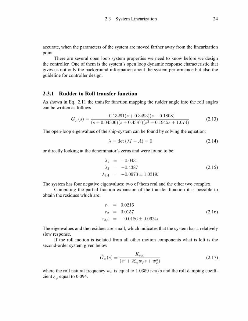
2.3.1 Rudder to Roll transfer functionAs shown in Eq. 2.11 the transfer function mapping the rudder angle into the roll anglescan be written as follows
G' (s) =�0:13291(s+ 0:3493)(s� 0:1808)
(s+ 0:04306)(s+ 0:4387)(s2 + 0:1945s+ 1:074)(2.13)
The open-loop eigenvalues of the ship-system can be found by solving the equation:
� = det (�I � A) = 0 (2.14)
or directly looking at the denominator's zeros and were found to be:
�1 = �0:0431�2 = �0:4387 (2.15)�3;4 = �0:0973� 1:0319i
The system has four negative eigenvalues; two of them real and the other two complex.Computing the partial fraction expansion of the transfer function it is possible to
obtain the residues which are:
r1 = 0:0216
r2 = 0:0157 (2.16)r3;4 = �0:0186� 0:0624i
The eigenvalues and the residues are small, which indicates that the system has a relativelyslow response.
If the roll motion is isolated from all other motion components what is left is thesecond-order system given below
~G� (s) =Kroll
(s2 + 2�'w's+ w2')(2.17)
where the roll natural frequency w' is equal to 1:0359 rad=s and the roll damping coef�-cient �' equal to 0.094.

2.3 System Linearization 25
2.3.2 Non-minimum Behavior in Ship ResponseIn the rudder-to-roll transfer function there are also two zeros;
q = �0:3493 (2.18)q1 = 0:1808
one of the two zeros is on the right-hand side of the complex plane - see Fig. 2.4. Thisresults in a limitation in the design of a control system [14]. In particular the positive zerodetermines a trade-off between reducing the roll at some frequencies and amplifying it atothers.
Root Locus
Real Axis
Imag
inary
Axis
1 0.8 0.6 0.4 0.2 0 0.2 0.4 0.6 0.8 11
0.8
0.6
0.4
0.2
0
0.2
0.4
0.6
0.8
1
Fig. 2.4. Poles and zeros of the rudder to roll transfer function.
If a positive step is sent in as an input to a system with a positive real zero at s = qsuch as G'(s) then the output response of the closed-loop system would be
Y (s) =G'(s)
1 +G'(s)
1
s= T (s)
1
s(2.19)
The single-sided (unilateral) Laplace transform for a signal x(t) is de�ned as
L [x(t)] = X(s) =
Z 1
0
e�stx (t) dt (2.20)

2.3 System Linearization 26
assuming that the integral can be evaluated at the upper and lower limits to yield well-de�ned and bounded values. Associated with this transform X(s), and equivalent to thestatement that the transform exists, is the signal's Region of Convergence (ROC). If thetransform exists, the ROC exists, and vice versa. The ROC is the open half of the s-planethat lies to the right of all singularities (poles) of X(s). At any point s = s0 that lies insidethe ROC, the following relationship is true.
X(s0) =
Z 1
0
e�s0tx (t) dt (2.21)
Therefore, at any point s = s0 in the region of convergence, the form of the de�ningequation of the Laplace transform is still applicable, with the complex variable s replacedby the complex number s0.
0 20 40 60 80 1002
1
0
1
2
3
4
time [s]
φ [d
eg]
Fig. 2.5. Non-minimum-phase effect on roll dynmamics during a turn to port.
In the problem being considered here, since the zero q is in the region of convergencefor the transform Y (s), applying the Laplace transform to y (t) and Y (s) with s0 = q itfollows that Z 1
0
e�qty (t) dt = Y (q) = T (q)1
q= 0 (2.22)
Since q is a real number, the exponential term inside the integral in Eq. 2.22 is alwayspositive. The output signal has an initial value y(0) = 0 and a �nal value y(1) = 1, soy(t) is not identically equal to 0. However, the results stated in Eq. 2.22 indicate that the

2.3 System Linearization 27
area under the curve of y(t) (weighted by a time-varying positive number) over all timeis equal to 0. Therefore, the output signal y(t) must take on negative values. This meansthat when the open-loop system has a right-half plane (nonminimum-phase) zero, the stepresponse spends part of its time going in the wrong direction. This is generally knownas a non-minimum-phase response or an inverse response. This inverse response alwaysexists when the closed-loop system has a right-half plane zero. Since zeros of the open-loop forward transfer function G(s) appear as closed-loop zeros, then whenever G(s) hasa non-minimum-phase zero, the system's step response will exhibit undershoot, taking onnegative values. It can be also noticed that the slower the system response is the larger willbe the initial system response. Fig. 2.5 illustrates this non-minimum-phase behavior forthe rudder-to-roll transfer function. The step response to a 10 degrees rudder angle inputgoes negative �rst, then goes positive, ending with the �nal value.

Chapter 3Environmental Disturbances
There are several disturbances with various effects on the vessel dynamics to be takeninto account. Mainly three classes of disturbances can be distinguished:
� Disturbances which affect the dynamics of the system, like for example the depth of
the water
� Disturbances which cause additional signals in the system such as waves
� Disturbances that corrupt the measurements like sensor noise.
3.1 Wind generated wavesEnvironmental disturbances such as waves, wind and current are the principal causes of theundesirable motion of the ship. For the problem at hand, only wind generated waves aretaken in account since they represent the dominant disturbance in the task of seakeeping.There are several models in literature to describe the phenomenon of wave generation.As described by Fossen [9] the process of wave generation due to wind starts with smallwavelets appearing on the water surface. These short waves starts and continue to growuntil they �nally break and their energy is dissipated. It has been observed that a developingsea, or storm starts with high frequencies. When a storm has lasted for a long period oftime is said to create a fully developed sea. After the wind has stopped, a low frequencydecaying sea is formed.
The objective of this section is directed to the description of wave spectra and shipmotion in waves. The response of a ship to waves is quite complex. Having a certainvelocity of advance, a ship experiences the wave excitation at an encounter frequency.This frequency is not related linearly to the wave frequency, as seen from a �xed point,but varies with ship speed and angle of attack from wave through a nonlinear mapping.Furthermore, forces and moments on the hull are determined by the wavelength of incidentwaves through a square root function of the wave frequency.
The mathematical description of the motion of regular gravity waves over a free sur-face is classical. A two dimensional wave progressing at an angle { with respect to theinertial frame, is described by its elevation � at a certain position x; y at time t
�(x; y; t) = �� sin(!0t� kx cos({)� ky sin({) + ") (3.1)
28

3.2 Stochastic representation 29
wherek = the wave number!0 = wave frequency�� = wave amplitude" = the initial phase angleThe phase velocity of the wave, c, is the velocity with which the wave crest move
relative to the ground. Assuming a gravity wave and in�nite depth of water, the followingdispersion relationships hold:
k =!20g
� =2�
kc =
rg�
2�(3.2)
where g is the acceleration of gravity, and � is the wavelength. The phase velocity isinversely proportional to its frequency. In other words, long waves propagate faster thanshort ones. This phenomenon is crucial for simulation of wave motion. A ship advancingin a seaway will overtake some short waves, while it will be overtaken by some long ones.A motion of the ship at a certain encounter frequency can, therefore, be caused by up tothree harmonic waves with three different wavelengths.
3.2 Stochastic representationWhen the wave amplitude and frequency become random variables the simple waves areextended to an irregular sea. Ocean waves are random in terms of both time and space.Therefore, a stochastic modelling description seems to be the most appropriate approachto describe them. It is assumed that the variations of the stochastic characteristics of thesea are much slower than the variations of the sea surface itself. Due to this, the elevationof the sea at a certain position �(x; y; t) can be considered as a realization of a stationaryprocess. Haverre and Moan [12] suggested the following simplifying assumptions aboutthe stochastic model:
� The observed sea surface, at a certain location and for short periods of time, is
considered a realization of a stationary and homogeneous, zero mean Gaussian
stochastic process.
� Some standard formulae for the spectral density function S(!) are adopted.
Under a Gaussian assumption, the process, in a statistical sense, is completely char-acterized by the power spectral density function S(!).
A conceptual model to describe the elevation of an irregular sea is given by the sumof a large number of essentially independent regular (sinusoidal) contributions with random

3.3 Nonlinear models of wave spectra 30
phases. Then the sea elevation at a location x; y is given by:
�(x; y; t) =
NXi=1
� i(x; y; t) =
NXi=1
�� i sin(w0it� kix cos({)� kiy sin({) + "i) (3.3)
where � i(x; y; t) is the contribution of the regular travelling wave components i progressingat an angle { and a with random phase "i. The above statements imply that the mean andthe variance of the waves elevation are
E [�(t)] = 0 (3.4)
var[�(t)] =
Z 1
0
S (!) d! (3.5)
3.3 Nonlinear models of wave spectraResearchers who have studied ocean waves have proposed several formulation for wavespectra dependent on a number of parameters (such as wind speed, fetch, or modal fre-quency) [23]. These formulations are very useful especially in the absence of measureddata, but they can be subject to geographical and seasonal limitations. Many models are nonlinear and determine the sea spectrum using spectral estimation techniques; they are usedto derive linear approximations and transfer functions for computer simulations. Based onextensive data collection, mostly in the North Atlantic ocean, a series of idealized singleside local spectra have been obtained to described long-crested seas. The most widely usedin maritime engineering are the Pierson-Moskowitz (PM) and the JONSWAP spectra. Theformer model takes the name from the developers of a two parameter spectral formulationfor fully developed wind generated seas. It has the following form:
S (!) = A!�5 exp(�B!�4); [m2s] (3.6)
where the parameters A and B are
A = 8:1 � 10�3g2
B =3:11
H2s
(3.7)
with Hs being the signi�cant wave height (mean of the one third highest waves) usedto classify the type of sea and g is the gravity constant. The signi�cant wave height isproportional to the square of the wind speed at 19.4 meters over the sea surface and theirrelationship is expressed here:
Hs =2:06
g2V 219:4 (3.8)
The modal frequency (peak frequency) !0 and modal period T0 for the PM-spectrum arefound requiring that �
dS (!)
d!
�!=!0
= 0 (3.9)

3.4 Linear approximations of wave spectra 31
and they are
!0 =4
r4B
5T0 = 2�
4
r5
4B(3.10)
The International Ship and Offshore Structures Congress (ISSC) and the InternationalTowing Tank Conference (ITTC) have suggested the use of a modi�ed version of the PM-spectrum. For prediction of responses of marine vehicles and offshore structures in opensea, they recommended to use the following parameters:
A =4�3H2
s
T 4z
B =16�3
T 4z(3.11)
where Tz = 0:710T0 is the average zero-crossing period.For non fully developed seas the PM-spectrum cannot be used; so it should be re-
placed by the Joint North Sea Wave Project (JONSWAP) spectrum. It was developed forthe limited fetch North Sea and is used extensively by the offshore industry. This spectrumis signi�cant because it was developed taking into consideration the growth of waves over alimited fetch and wave attenuation in shallow water. Over 2,000 spectra were measured anda least squares method was used to obtain the spectral formulation assuming conditions likenear uniform winds. The JONSWAP spectral density function will result in a more peakedfunction than those representing fully developed seas. Many other spectra have been ob-tained and which are not discussed: these include the Neumann, the Bretschneider, theOchi and the Torsethaugen spectra.
3.4 Linear approximations of wave spectraA method commonly used in control for analysis and simulation is to replace the nonlinearwave disturbance model with a linear wave response approximation [9]. A linear approxi-mation of the shape of the power spectral density function of the signal of interest is givenby
Syy(j!) = jH(j!)j2 Sww (j!) (3.12)where Sww is the power spectrum of a zero-mean Gaussian white noise process which isconstant and equal to one. The �lterH (s) is called a shaping �lter and can be implementedin several ways (different orders and structure) but the most commonly used is the second-order �lter of the form:
H (s) =2�!0�s
s2 + 2�!0s+ !20(3.13)
where � is a damping coef�cient, � is a constant describing the wave intensity, and !0 isthe dominating wave frequency.
Hence, substituting s = j! into Eq. 3.13
H (j!) =j2�!0�!
!20 � !2 + j2�!0!(3.14)

3.4 Linear approximations of wave spectra 32
The square of the magnitude of the �lter is then easily obtained:
jH (j!)j2 = 4�2!20�2!2
(!20 � !2)2+ 4�2!20!
2(3.15)
0 0.2 0.4 0.6 0.8 1 1.2 1.4 1.6 1.8 20
0.4
0.8
1.2
1.6
2 Wave spectrum
ω [rad/s]
S( ω
) [m
2 s]
PM spectrumLinear spectrum
Fig. 3.1. Power spectrum of the linear approximation and the Pierson-Moskovitz model.
As it is from the Pierson-Moskowitz spectrum when ! is equal to the dominatingwave frequency !0; the maximum value of Syy(jw) can be obtained as
max!
Syy(!) = Syy(!0) = �2 (3.16)
The dominating frequency in the linear model is also equal to the modal frequency of thePM spectrum
!0 =4
s4 � 16�35T 4z
(3.17)
The Power spectrum of the linear approximation (solid line) and the one of Pierson-Moskowitzmodel (dash) for the same signi�cant wave height Hs = 4, period T0 = 8s, and dampingcoef�cient � = 0:25 are plotted in Fig. 3.1.

3.5 Encounter frequency 33
3.5 Encounter frequencyWaves incident on the structure of a ship can be described as head seas, following seas,beam seas, quartering seas or bow seas depending on the incident direction. Fig. 3.2illustrates the different cases. The incident angle, �, is measured from the stern.
Fig. 3.2. Incident sea description. Courtesy of NTNU [21].
The motion of a ship, forward or otherwise, affects the way incident waves are viewedby someone aboard the vessel. For example if the ship is making way in following seaswith a constant velocity, u, then the waves will appear to meet the ship at a slower rate thanthe actual frequency of the waves. This new, or observed, frequency is called the encounterfrequency,!e. If the waves are incident on the ship at some angle, �, then the componentof the speed of the ship in the direction of wave propagation is uw = u cos (�). The wavecrests move at the phase speed, c =
!
kand the relative speed between the ship and the
waves isur = c� uw =
!
k� u cos (�) (3.18)
Using the dispersion relationship for waves in deep water it is possible to rewrite the equa-tion for encounter frequency as
!e = ! � !2u
gcos (�) (3.19)

3.6 Waves simulation model 34
Fig. 3.3 shows a schematic representation of the transformation between ! and !efor different sailing conditions and u constant. From this �gure, it can be seen that whenthe vessel is sailing in bow or head seas the wave frequencies are mapped into higherfrequencies. In beam seas, however, there is no change and both ! and !e are the same. Infollowing and quartering seas, the situation becomes more complicated as different wavefrequencies can be mapped into the same encounter frequency.
Fig. 3.3. Encounter frequency versus actual frequency.
3.6 Waves simulation modelTo simulate the elevation of the sea surface for a fully developed condition the Simulinkblock diagram reproduced in Fig. 3.4 has been used. The band limited white noise used inthe simulation has a power spectral density equal to one.
Figure 3.5 shows the signal representing the wave disturbance generated using theSimulink blocks. The stochastic disturbance has been plotted for a period of three minutes.The values used are: wave height Hs = 1:5m, period T0 = 8s, and damping coef�cient

3.6 Waves simulation model 35
Fig. 3.4. Simulink block diagram for wave disturbances.
� = 0:25. The disturbance has been considered as an output disturbance and hence addedto the roll angle signal of the ship system.
0 50 100 150 200 250 3003
2
1
0
1
2
3
time [s]
wav
e he
ight
Fig. 3.5. Wave disturbance simulation

Chapter 4Ship Roll Stabilization
There are numerous reasons for trying to control and reduce the motions of a ship.Excessive motions can interfere with the activities of the crew or passengers, reduce thecombat readiness of naval vessels, cause the loss of containers on cargo vessels, and reducethe operational parameters of various ships. From a safety point of view it is importantfor critical marine operations like landing a helicopter, formation control or underway re-plenishment. Over the years, many types of motion control or reduction devices have beendevised. Most of them have been aimed at reducing roll motions since the force requiredto reduce roll is reasonably small compared to the weight of the ship. Moreover, roll is thelargest and most undesirable component of ship motion.
The �rst step in a good roll stabilization is a careful hull design and subsequentlyintelligent load distribution. It has been studied and showed [10] that what excites therolling motion of a ship is not the height of the wave but the steepness (or slope). Sinceshort waves appear to be steeper than long waves, it has been noticed that the roll period ofthe vessel should be extended as much as possible to avoid synchronization with the waveexcitation frequency. This is done, as suggested by Perez [22], by increasing the momentof inertia (load distribution on the ship) and reducing the transverse stability (shape of thehull and load).
Even though several efforts have been made in this direction, it is impossible to avoidthat waves will excite roll for some sailing conditions. For these reasons, the vessel isoften equipped with various roll reduction systems including gyroscopic stabilizers, anti-roll tanks, bilge keels, �ns, moving weights, and active rudder control. Most of thesemethods �rst started as passive control and then evolved into active control.
4.1 Stabilizing MethodsAn overview [32] of the working characteristics of some of the most commonly used sta-bilizer devices is here provided.
Gyroscopes: It is a spinning wheel or disk whose axle is free to take any orientation.This orientation changes much less in response to a given external torque than it wouldwithout the large angular momentum associated with the gyroscope's high rate of spin.This type of stabilizer uses the effects of the large rotating wheel to generate a reducingmoment. This method was meant to eliminate roll rather than to reduce it but it is not inuse anymore.
Anti-roll tanks: This system utilizes the motion of water located in connected tanks.The motion of the ship causes the water to move from tank to tank, and the tank connectionis tuned such that the motion of the water resonates out of phase with the roll motion. Themost widely used anti-roll tank is the U-tube tank, which is composed of two reservoirs,
36

4.1 Stabilizing Methods 37
located one on port and one on starboard, connected at the bottom by a duct as shown inFig. 4.1.
Fig. 4.1. Examples of U-tube tanks. Courtesy of Yang [32].
This method has a medium to high performance independently of the operation speedof the vessel and does not need great maintenance work. As drawbacks it has to be men-tioned that anti-roll tanks can affect the stability of the vessel due to free-surface effects(the tank is not full and there is space for the water to move.) and that they occupy largespaces.
Bilge keels: It is the simplest form of stabilizers consisting of two keels that emergeat an angle from the hull of a sailboat, at or near the bilges. The longitudinal extent mayvary from about 25 to 50 percent of the length of the ship. Bilge keels increase the hulldamping by generating drag forces which act perpendicular to the keels and oppose theroll motion. They are widely used, are inexpensive, easy to install but they increase theresistance in calm water and not all ships can be �tted with them. Their performance is inthe range of 10-20 percent of roll angle reduction.
Fins: Fin stabilizers consist of a pair of wings mounted on rotatable stocks at theturn of the bilge located about amidships. The ship roll is sensed via gyroscopes and fedback to the control system, which commands the actuator to modify the angle of incidence

4.1 Stabilizing Methods 38
of the �ns. They provide considerable damping if the speed is not too low; estimated in therange of 60-90 percent of roll reduction. The disadvantages are however many: high costassociated with the installation, few ef�ciency at low speed, need of sensors and powerfulactuators, increase of resistance, easily damaged and with high risk of grounding in shallowwater. - see Fig. 4.2.
Fig. 4.2. Fin stabilizer arrangement.
Rudder : This technique is based on the fact that the rudder is located aft and alsobelow the center of gravity of the vessel and thus it imparts not only yaw but also rollmoment. This stabilization method can be implemented on different ship types: smalland large naval vessels, patrol and �shing vessels, ferries and some ro-ro vessels (roll-on/roll-off ships, which are designed to carry wheeled cargo such as automobiles, trailersor railroad cars). The rudder roll stabilization system is nowadays one of the primary rollcontrol devices in use and this is due to its numerous advantages:
� Medium to high performance (50 to 70 percent).
� Low life cycle cost.

4.2 Rudder Roll Damping Control Systems 39
� No extra weight.
� High stabilizing performance.
� Optimal propulsion performance.
� No additional equipment required.
� Space saving arrangement.
� Low hydroynamic resistance, no underwater acoustic signature.
� Can be combined with other stabilizers.
The disadvantages are its ineffectiveness at low speed, the fact that drag is producedwhen in use, the need of rudder machinery up-grade and of sophisticated control systems.
In the following sections some methods for roll stabilization using the rudder areintroduced. The main motivation for using roll stabilizing systems on ships, as alreadymentioned above are to prevent cargo damage and to increase the effectiveness of the crewby avoiding or reducing seasickness.
4.2 Rudder Roll Damping Control SystemsThe main objective in roll damping is to minimize the wave impact on ship motions, ex-pressed as the p and ' components. By providing a state feedback, making the systemclosed-loop, it is possible to put an input to the system that represents the desired outputor state, and the controller becomes responsible for reaching the desired values. In thiscase the input to the system will no longer be the control signals for the rudder, but the rollangle. The controllability matrix of the ship system has full rank, which means that it iscontrollable. The basic structure of the RRD system used in this simulation can be repre-sented by the block diagram shown in Fig. 4.3. The reference signal 'ref is set to zero,which indicates the desired stabilized horizontal position.
Following the scheme of Fig. 4.3 different controllers have been designed in order toachieve a good roll reduction. In the next sections the design, implementation and resultsof these controllers are shown.

4.3 Sensitivity function 40
Fig. 4.3. Rudder roll stabilization (RRS) system structure
4.3 Sensitivity functionOne of the performance objectives of controller design is to keep the error between thecontrolled output and the set-point as small as possible, when the closed-loop system isaffected by external signals. Thus, to be able to assess the performance of a particular con-troller, it is needed to be able to quantify the relationship between this error, the process andthe controller [24]. In this work the sensitivity function has been chosen as a quantifyingmeasure.
S (s) =' (s)
d (s)=
1
1 + C (s)G' (s)(4.1)
This function has an important role to play in evaluating the performances of the controllerbecause it also describes the effects of the disturbance, d (s) ; on the controlled output,' (s). The function has been named by Bode because it gives the relative sensitivity of theclosed loop transfer function T (s) to the relative plant model error.
T (s) =C (s)G' (s)
1 + C (s)G' (s)(4.2)
Equation 4.2 represents the complementary sensitivity function which in case of a noisefree system relates the controlled variable ' (s) to the desired output 'ref (s). In particular,at a given frequency ! for a single input single output plant the relation between the two

4.4 Ship motion performance 41
functions is the followingdT=T
dG'=G'
= S (4.3)
From the requirement of good disturbance attenuation, the following is needed
jS (j!)j << 1 (4.4)
Another typical performance speci�cation for a robust control is then the sensitivity func-tion does not exceed the superior limit of one or in other terms
sup (jS (j!)j) � 1 (4.5)
The sensitivity function will be studied in order to improve the system performance, and tosurvey the stability of the system.
4.4 Ship motion performanceWhen stabilizers are implemented there is the need to develop some methods or �guresto investigate the ef�ciency of such controllers. Perez gave an overview of some of thesemethods [22]. Different manufacturers can chose different ways to show the achievableperformances. This can generate some confusion when it comes to compare various sys-tems. Although the possibilities are quite many in this section the most widely used �guresare presented.
4.4.1 Reduction of Roll at Resonance-RRRIf the ship roll motion is compared to a mass spring damper system, the moment of inertiain roll can be the mass component, the spring is given by the buoyancy and gravity forcestending to restore the equilibrium position, and the damping arises from the interaction be-tween the hull and the water. Thus under these assumptions the ship response to wavespresents a resonant peak. This method of quantifying the performance consists in evalu-ating the roll reduction at the roll resonant frequency !' for a sinusoidal wave excitation,with a wave encountering the ship from the beam:
RRR = 100
�1� �'on
�'off
�!e=!'
(4.6)
where �' denotes the peak value of the roll angle and the subscripts indicate wether thecontroller is switched on or off. This type of �gure is very popular among stabilizer becauseit usually shows great performance of the system. In fact this type of measurement tends tooverestimate the actual roll reduction obtained in a seaway, in which the waves have energydistributed over a range of frequencies rather than at a single one. For these reasons this�gure is not taken in consideration in the performance results of this work.

4.4 Ship motion performance 42
4.4.2 Reduction of Statistics of Roll -RSRThis method is probably the one that gives the most accurate results in estimating the rollreduction. In fact since the roll motion varies according to the sea state and sailing condi-tions it is more appropriate to evaluate the performance using statistics for different situa-tion. There is not only one statistics that can be taken in account. The expression of thepercentage reduction of statistics of roll is de�ned as
RSR = 100
�1� Son
Soff
�(4.7)
and S can be one of the following statistics of roll motion:
� Variance: var (')
� Root Mean Square (RMS) value: 'RMS =pvar(')
� Signi�cant Amplitude (SSA): 'SSA = 2pvar(')
The square root in the last two statistics indicates that the RSR results in a higherroll reduction �gure for variance than for RMS and SSA.
4.4.3 Reduction of Probability of Roll Peak Occurrence -RROThis method introduces a different approach in considering the roll reduction. If the rollmotion is considered as a narrow-banded Gaussian stochastic process (response to stochas-tic wave excitations) this �gure represents the probability, for the maxima of a realizationof roll angle �'i, of exceeding a certain value of the roll angle '�.
The above described probability is given by
P (�' > '�) =
Z 1
'�
�'
var (')exp
�� �'2
2var (')
�d�' = exp
� ('�)2
2var (')
!(4.8)
where the integrand in Eq. 4.8 is the so called continuous Rayleigh probability densityfunction - see Fig. 4.4. In order to obtain the percentage of time in which the roll angleexceeds a given value during a certain period it is necessary to multiply Eq. 4.8 by 100.Then the Reduction of Probability of Roll Peak Occurrance-RRO is de�ned as:
RRO('�) = 100
�1� P (�'on > '�)
P (�'off > '�)
�= 100
�1� exp(�F ('�)2)
�(4.9)
with
F =1
var('on)
�1� var('on)
var('off )
�(4.10)

4.4 Ship motion performance 43
0 1 2 3 4 5 60
0.5
1
1.5
2
2.5
3
3.5
x
f(x,s
igm
a)sigma = 0.2sigma = 0.5sigma = 1sigma = 2
Fig. 4.4. Rayleigh probability density function
Equation 4.9 should be interpreted as the probability of occurrence of maximum roll anglesexceeding the given threshold angle '�. This �gure is very useful when it is necessary toestimate the advantages of the stabilizers in case the roll angle is not wanted to exceedcertain values.

Chapter 5Cheap limiting optimal control
An optimal control deals with the problem of �nding, for a given system, a controllaw u (x) belonging to a class of admissible controls U such that it minimizes a cost func-tion J , associated with the system _x = f (x; u). There are various types of optimal controlproblems, depending on the performance index, the time domain (continuous, discrete), thepresence of different kind of constraints, and which variables are free to be chosen.
The formulation of the optimal control problem is usually posed as
minuV (x; u; �)
subject to u2U and _x=f(x;u)
(5.1)
where � is a vector of weighting parameters. Then, uopt is said to be the optimal control if
V (x; u; �) � V�x; uopt; �
�8u 2 U (5.2)
and it is denoted asuopt = argu2U minV (x; u; �) (5.3)
The optimal cost is thenV opt (x; �) = min
u2UV (x; u; �) (5.4)
It is said to be limiting if the cost to be minimized becomes a function of either the state orthe control action but never of both.
5.1 Minimum Variance Cheap ControlThis particular case considers a cheap limiting optimal control, since the weight of thecontrol effort in the cost tends to zero. Even if the control is cheap and there is no costassociated with using large control action the cost function cannot be reduced to zero. Forthe rudder-to-roll transfer function G� (s) the goal is to �nd a proper stabilizing controllerC (s) that minimizes the performance index
J = lim�!0
var [y] + �var [u] (5.5)
The only disturbance taken in consideration is the output disturbance, which is aWide Sense Stationary stochastic process. As already discussed in Chapter 3, it can beapproximated as �ltered white noise n with constant PSD Snn for �1 < ! <1:
Sdd (!) � jH (j!)j2 Snn (5.6)
By de�nition the power spectrum of a continuous-time stochastic process x (t) is the Fouriertransform of its autocovariance function
Sxx (!) =
Z +1
�1Cxx (�) e
�j!�d� (5.7)
44

5.1 Minimum Variance Cheap Control 45
According to Perez [22], beingG' (s) a stable SISO plant with one NMP zero q 2 R+then the minimum value of the Cost is
minV = 2q jH(q)j2 Snn (5.8)
Using the Youla Parametrization it is possible to write a controller in the following way[11]:
C (s) =Q (s)
1�G' (s)Q (s)(5.9)
from which it follows that the sensitivity function can be written as
S (s) = 1�G(s)Q(s) (5.10)
Using the Fourier transform pair between autocorrelation and power spectral density thevariance of the output can be written as:
var [y] = Cyy (0) =1
2�
Z +1
�1Syy (!) d!
=1
2�
Z +1
�1jH (j!)j2 j1�Q (j!)G (j!)j2 Snnd!
=Snn2�
Z +1
�1jH (j!)�Q (j!)H(j!)G (j!)j2 d! (5.11)
= Snn jjH (j!)�Q (j!)V (j!)jj22where the equality in Eq. 5.11 has been obtained with the use of the H2 norm and consid-ering
V (j!) = H (j!)G (j!) (5.12)It is possible to factorize the last term as follows
V (j!) = (H (j!)Gm (j!))
�s� q
s+ q
�= Vm (j!)Va(j!) (5.13)
whereGm (s) and Vm (s) have no poles or zeros in the right hand side of the complex plane.Manipulating the expression of the output variance using the results of the factoriza-
tion and noting that jVa (s)j = 1, it can be written as:
var [y] = Snn����Va (j!) �Va (j!)�1H (j!)�Q (j!)Vm (j!)
�����22
= Snn����Va (j!)�1H (j!)�Q (j!)Vm (j!)
����22
(5.14)
= Snn�����Va (j!)�1H (j!)�u + �Va (j!)�1H (j!)�s �Q (j!)Vm (j!)
����22
where the subscripts s and u stand for the stable and the unstable part of the expressioninside the rectangular brackets and they are calculated as follows:
Va (s)�1H (s) =
s+ q
s� q� 2�!0�s
s2 + 2�!0s+ !20=
�
s � q| {z }unstable
+�s+
s2 + 2�!0s+ !20| {z }stable
(5.15)

5.1 Minimum Variance Cheap Control 46
Noting that�Va (j!)
�1H (j!)�uand
�Va (j!)
�1H (j!)�s�Q (j!)Vm (j!) are orthogonal
the whole expression can be rearranged as
var [y] = Snn�����Va (j!)�1H (j!)�u����22
+Sww�����Va (j!)�1H (j!)�s �Q (j!)Vm (j!)
����22
(5.16)
From Eq. 5.16 it can be seen that the Q (s) that minimizes the cost function is
Q (s)opt = Vm(s)�1[Va (j!)
�1H (j!)]s (5.17)
The wave response linear approximation �lter H (s) used to reproduce the wave dis-turbance has been used in the design of the controller. The peak of its spectrum has beenchosen at a frequency of
�
4rad/s corresponding to a wave period of eight seconds. The bode
plot of the linear approximation wave disturbance �lter for !0 and � respectively equal to�
4and 0.25 is shown in Fig. 5.1.
102
101
100
101
102
0,01
0,1
1
4
ω [rad/sec]
|H(j ω
)|
Bode Diagram
Frequency (rad/sec)Fig. 5.1. Bode plot of wave disturbance �lter H(s)
Looking at the Eq. 2.11 describing the ship system, the function V (s) can be writtenas follows
V (s) =Kroll(q � s)(q1 + s)
(p1 + s)(p2 + s)(s2 + 2�!rolls+ !2roll)� 2�!0�s
s2 + 2�!0s+ !20(5.18)

5.1 Minimum Variance Cheap Control 47
From Eq. 5.18, knowing that Va (s) is the all pass term introduced in Eq. 5.13, it is theneasy to obtain the formulation for Vm(s). In fact it is the same as V (s) with the onlydifference that the positive zero (q � s) has been substituted by (q + s).
Vm (s) =Kroll(q + s)(q1 + s)
(p1 + s)(p2 + s)(s2 + 2�!rolls+ !2roll)� 2�!0�s
s2 + 2�!0s+ !20(5.19)
The stable and unstable part of Va (s)�1H (s) are already de�ned in Eq. 5.15. The �nalexpression for the optimal Q is hence achieved
Q (s)opt =
�Kroll(q + s)(q1 + s)
(p1 + s)(p2 + s)(s2 + 2�!rolls+ !2roll)� 2�!0�s
s2 + 2�!0s+ !20
��1� �s+
s2 + 2�!0s+ !20(5.20)
=(p1 + s)(p2 + s)(s2 + 2�!rolls+ !2roll)
Kroll(q + s)(q1 + s)��
�s+
�
�2�!0�s
The obtained transfer function for the optimal Q is found but the transfer function of thecontroller derived from this optimal solution becomes improper having �ve zeros and onlythree poles as it can be seen from Eq. 5.21.
C (s) =
Kc(p1 + s)(p2 + s)(s2 + 2�!rolls+ !2roll)
�s+
�
�(q1 + s)(s2 + 2�!0s+ !20)
(5.21)
To have an understanding of the behavior of the designed controller, it is helpful toconsider the output sensitivity function described previously. From the plot of this func-tion in Fig. 5.2 it can be noticed that the desired performances are reached. The maximumdamping is obtained around the disturbance frequency !0 with a magnitude of 0:025mean-ing that the system is able to reduce the roll motion for that particular frequency almostentirely. This value clearly shows that this kind of approach can result in very successfulperformances. Even though it is true that for frequency close to !0 it is possible to obtaingood disturbances rejection it is also evident that the system designed in such a way is notable to reduce the low frequency disturbances or at least leave them unchanged: it insteadampli�es them enormously. For low frequencies 0:05 � ! � 0:1 the roll motion is aug-mented from two to �ve times and for very low frequencies ! � 0:02 even ten or twentytimes.
As already pointed out the �nal controller is improper meaning that the order ofthe numerator is higher than the order of the denominator. This leads to the fact that acontroller characterized by that type of transfer function wouldn't be feasible in the realworld. However this impasse can be overcome by making a proper approximation addingstable fast poles. The poles that must be added to render the function bi-proper are two andthey have been placed after the disturbance frequency !0:The main problem with choosingthe poles at the right frequency was that if poles at higher frequencies were chosen they

5.1 Minimum Variance Cheap Control 48
102
101
100
101
102
0,1
1
10
40
ω [rad/sec]
|S(j ω
)|
Bode Diagram
Frequency (rad/sec)
C(s) improperC(s) biproper
Fig. 5.2. Sensitivity function for the proper and improper cheap controller.
yielded a controller with higher magnitude. In fact even if the damping range would beincreased the resulting controller would generate some problems for what concerns thelimit on the maximal rudder angle and slew rate. The system would eventually saturatedue to the high gain of the controller and produces really poor performances for the rollreduction. The realizable controller has the form of
C (s) =
Kc(p1 + s)(p2 + s)(s2 + 2�!rolls+ !2roll)
�s+
�
�(q1 + s)(s2 + 2�!0s+ !20)(pf + s)2
(5.22)
Once the �rst step is accomplished with the add of two fast poles the controller expressedin Eq. 5.22 still has to be modi�ed to achieve its speci�cations. The second and mostimportant problem, as already discussed, is that at low frequencies the disturbances areampli�ed. Instead it would be at least desirable that the controller leaves the disturbancesat those frequencies untouched allowing the sensitivity function to assume values aroundthe unity. It was therefore necessary the use of a high pass �lter formulated as
Fhp =Ts
T1s+ 1(5.23)

5.2 Stability and Performance Trade-offs 49
to force the system to the desired behavior. The expression of the controller with this lastchange becomes the following
C (s) =
Kc(p1 + s)(p2 + s)(s2 + 2�!rolls+ !2roll)
�s+
�
�(q1 + s)(s2 + 2�!0s+ !20)(pf + s)2
� Ts
T1s+ 1(5.24)
5.2 Stability and Performance Trade-offsDifferent values for the �lter have been tried in order to achieve the best performance forthe designed controller. Taking a glance at the frequency plot of the output sensitivityfunction in Fig. 5.4 it is possible to understand the limitation that this kind of approachintroduces. When it comes to the design of a rudder roll stabilizer, there is the risk thatfor some sailing conditions and sea states, the disturbances have signi�cant energy in thefrequency range where roll is ampli�ed. This limitations have been identi�ed since the�rst rudder stabilizers were implemented. To avoid these kinds of risk a trade-off has to bereached between a good reduction at the desired frequency and a value as close to unity aspossible for the other frequencies. This can be done by choosing different values for the�lter and by looking at the different results obtained.
1.5 1 0.5 0 0.5 11.5
1
0.5
0
0.5
1
1.5Nyquist Diagram
Real Axis
Imag
inary
Axis
1.5 1 0.5 0 0.5 11.5
1
0.5
0
0.5
1
1.5Nyquist Diagram
Real Axis
Imag
inary
Axis
Fig. 5.3. Nyquist plots of L(j!) for the unstable and stable plant.
The trade-off must take in consideration that the most critical issue in designing feed-back controllers is to achieve stability. If the feedback gain is too large, then the controllermay overreact and the closed-loop system becomes unstable. This phenomenon is morelikely to happen with a model presenting a right-half plane zero such as the rudder angle

5.2 Stability and Performance Trade-offs 50
to roll angle system. It is useful to point out that a high pass �lter such as the one intro-duced in expression 5.23 leads to a closed loop instability when the ratio between T and T1is higher than a certain value. It is therefore necessary to keep in mind this constraint whenthe ef�ciency of the controller is discussed. Figure 5.3 shows the stable and the unstableclosed loop systems obtained by changing the T and T1 ratio. After a series of trials anderrors it can be clearly noticed that the better the low frequency constraint is ful�lled thelower roll damping at the interesting frequencies is achieved. Viceversa the best reductionperformance close to the disturbance frequencies is obtained with the drawback of a distur-bance ampli�cation for other frequencies. Figure 5.4 makes perfectly clear the concept sofar conveyed.
102
101
100
101
102
0.2
0.5
1
2
4
ω [rad/sec]
|S(j ω
)|
Bode Diagram
Frequency (rad/sec)
Fig. 5.4. Cheap controller sensitivity function varying the ratio between T and T1.
By weightening the ratio of the terms of the �lter it is possible to make the systemdamping bigger. However since the area above the unity line is equal to the area belowthe unity line it also yields an increase of the ampli�cation of the other frequencies. Theoptimal solution is found for a speci�c ratio between T and T1.

5.2 Stability and Performance Trade-offs 51
5.2.1 Output varianceSince the disturbance is treated as a random process, to fully characterize its properties it isconvenient to look at its nth-order moments; more precisely the �rst order moment, meanor expected value and the centered second order moment variance. If the random processx (t) is considered than the nth-order moment is de�ned as
Mnx (t) =
Z +1
�1xnp (x; t) dx (5.25)
with p (x; t) being the probability density function [5]. In the design of the controllerthe output disturbance has been represented as a �ltered white noise with constant PowerSpectral density. The variance of the white noise is easily computed as
var(n) = �2n =1
2�
Z +1
�1Snn (!) d! (5.26)
It has been seen in Eq. 5.11 that the variance of the output is calculated as
var(y) = �2y =1
2�
Z +1
�1Syy (!) d! (5.27)
with
Syy (!) = SS�Sdd (!) = jH (j!)j2 SS�Snn (!) (5.28)
and S being the sensitivity function.To show some characteristics of the system after the implementation of the cheap
controller it is meaningful to look at the response of the close-loop systems at the varyingof the frequency. Figure 5.5 shows the ratio between the square root of the output varianceand the square root of the white noise variance. The value of the variance of the white noiseis always the same. The graph has been obtained by varying the frequency of the linear �lterrepresenting the wave disturbance, whereas the other parameters were kept constant. Forevery frequency the two variances were calculated. It is thus evident that the variance ofthe output reaches its lowest value for a certain frequency. It then starts growing as soon asthe frequency increases or decreases from that value. This frequency is really close to thefrequency with which the wave disturbance has been modelled.

5.3 Numerical simulations and results 52
0.6 0.8 1 1.2 1.40,3
0,35
0,4
0,45
0,5
0,55
0,6
ω [rad/s]
σou
t/ σw
ave
Fig. 5.5. Ratio between the output variance and the white noise variance for different fre-quencies.
5.3 Numerical simulations and resultsThe controller C(s) de�ned by Eq. 5.24 can be computed as
C(s) =�67:3329s(s+ 0:4387)(s+ 0:3404)(s+ 0:04306)(s2 + 0:1945s+ 1:074)
(s+ 0:3493)(s+ 0:01429)(s2 + 0:3926s+ 0:6166)(s+ 2:5)2
(5.29)Equation 5.29 was obtained choosing of two fast poles located at a frequency of 2.5 rad/sand a high pass �lter with values for T1 and T2 equal to respectively 10 and 70. Conse-quently the output sensitivity function S(s) de�ned by Eq. 5.10 assumes the followingform
S(s) =(s+ 0:01429)(s+ 2:5)2(s2 + 0:3926s+ 0:6166)
(s+ 0:01685)(s2 + 0:3656s+ 0:2079)(s2 + 5:024s+ 15:72)(5.30)
From its plot shown in Fig. 5.6 it can be observed that the center frequency at which thefunction assumes its lowest value is located at 0:9 rad/sec. Hence, an effective roll reductioncan be expected for a wave disturbance with dominating frequency around that frequency.

5.3 Numerical simulations and results 53
102
101
100
101
102
0,2
0,5
1
2
4
ω [rad/sec]
|S(j ω
)|
Bode Diagram
Frequency (rad/sec)
Fig. 5.6. Cheap controller system sensitivity function.
The performance of the controller in the sea-way is simulated for different distur-bances conditions. The simulations conditions together with the results obtained are pre-sented in the following pages. More precisely three different waves period have been stud-ied. Figure 5.1 shows the different sea conditions for a wave period of 6 seconds, Fig. 5.2for a 8 seconds wave period, and Fig. 5.3 for a 10 seconds wave period. According to thedescription made in Section 3.5 the different encounter frequency have been calculated forthe constant speed of 8 m/s and the considered angles of encounter. The RMS and RSRvalues are obtained using Eq. 4.7.
Encounter angle for T = 6s !e RMS RSRQuartering sea 0.415rad/s 12% 21%Beam sea 1.047rad/s 65% 88%Bow Sea 1.679rad/s 26% 45%Head Sea 1.941rad/s 14% 25%
Table 5.1. Cheap controller performances for a 6 seconds period wave disturbance

5.3 Numerical simulations and results 54
Encounter angle for T = 8s !e RMS RSRQuartering sea 0.429 rad/s 18% 33%Beam sea 0.785rad/s 66% 88%Bow Sea 1.141rad/s 63% 86%Head Sea 1.288rad/s 57% 81%
Table 5.2. Cheap controller performances for a 8 seconds period wave disturbance
Encounter angle for T = 10s !e RMS RSRQuartering sea 0.407rad/s 10% 18%Beam sea 0.628rad/s 57% 81%Bow Sea 0.856rad/s 68% 90%Head Sea 0.950rad/s 67% 89%
Table 5.3. Cheap controller performances for a 10 seconds period wave disturbance
The results of three particular cases are plotted in Fig. 5.7, 5.8 and 5.9. In the �rstgraph the roll angle with (black line) and without (blue line) the controller are plotted. Thefollowing plots reproduce in order the roll rate, the yaw angle the rudder angle, and theship speed. It is clear from the Figures that the rudder roll controller makes the steadycourse keeping deteriorate. This is obvious because the movement of the rudder modi�esnot only the roll angle as expected but also the yaw angle as in its basic purpose. This isone of the trade-offs that it is necessary to accept: the larger the rudder angle the biggerthe course deviation. The best performances have been achieved for frequency around 0.9rad/s with a roll reduction equal to 68% in RMS value and 90% in RSR value. For very lowfrequencies, which were obtained for Quartering seas the results were not as good: theyvaried from a reduction of 10% to 18% RMS and 18% to 33% RSR. The same issue wasnoticed for higher frequencies as in the case of Head seas or Bow seas with a wave periodof 6 seconds. The achieved damping did not go over the RMS value of 26%. The rudderangle never exceeded its magnitude and velocity limitations. From the plots it is possibleto realize that the use of the rudder as a roll damping device introduces a slight change inthe ship speed.

5.3 Numerical simulations and results 55
0 50 100 150 200 250 3005
0
5φ
[deg
]
0 50 100 150 200 250 3005
0
5
p [d
eg/s
]
0 50 100 150 200 250 30010
0
10
ψ [d
eg]
0 50 100 150 200 250 30020
0
20
δ [d
eg]
0 50 100 150 200 250 3007.95
8
8.05
time [s]
u [m
/s]
Fig. 5.7. Simulation at Bow seas with wave period of 6 seconds.

5.3 Numerical simulations and results 56
0 50 100 150 200 250 3005
0
5φ
[deg
]
0 50 100 150 200 250 3005
0
5
p [d
eg/s
]
0 50 100 150 200 250 3005
0
5
ψ [d
eg]
0 50 100 150 200 250 30020
0
20
δ [d
eg]
0 50 100 150 200 250 3007.95
8
8.05
time [s]
u [m
/s]
Fig. 5.8. Simulation at Beam seas with wave period of 8 seconds.

5.3 Numerical simulations and results 57
0 50 100 150 200 250 3005
0
5φ
[deg
]
0 50 100 150 200 250 3005
0
5
p [d
eg/s
]
0 50 100 150 200 250 3005
0
5
ψ [d
eg]
0 50 100 150 200 250 30020
0
20
δ [d
eg]
0 50 100 150 200 250 3007.95
8
8.05
time [s]
u [m
/s]
Fig. 5.9. Simulation at Head seas with wave period of 10 seconds.

5.4 Cheap controller robustness 58
For the roll damping system another key measure of effectiveness is the roll reductionratio, RRR. This informative measure for the roll motion reduction is:
RRR (!) =j' (!) + 'w (!)jonj' (!) + 'w (!)joff
(5.31)
Figure 5.10 plots the roll reduction ratio for wave periods from 3 to19 seconds.
4 6 8 10 12 14 16 18 200.2
0.4
0.6
0.8
1
wave period [sec]
roll
angl
e re
duct
ion
Fig. 5.10. Cheap controller roll reduction ratio as function of wave period.
5.4 Cheap controller robustnessThe results depicted in the previous section shows that for that particular system the perfor-mance objectives are satis�ed. An interesting possibility is then to look how this nominalmodel used for the design is able to withstand small differences and changes from thatspeci�c representation.
In control theory a system, organism or design may be said to be "robust" if it iscapable of coping well with variations (sometimes unpredictable variations) in its operatingenvironment with minimal damage, alteration or loss of functionality.
The �rst change in the system has been implemented on the constant speed �u. It hasbeen varied from 6 m/s (yellow line) to 10 m/s (black line) and the reduction ratio for the

5.4 Cheap controller robustness 59
roll angle for different wave periods has been calculated. The different results have beenplotted in Fig. 5.11. Ship speed variation changes roll angle damping from 0.27 to 0.42 ora factor 1.55 over the parameter envelope for a 7 seconds wave. The faster the ship travelsthe higher effect the rudder induced moment has on the roll diminution. The system hasstill good results for a small change of the constant speed. However if the speed variesto much from the nominal value these results cannot be expected anymore and differentcontrollers need to be implemented. In the task taken in discussion this factor is not of bigconcerns because ships are supposed to maintain a constant speed during their cruise.
4 6 8 10 12 14 16 18 200.2
0.4
0.6
0.8
1
wave period [sec]
roll
angl
e re
duct
ion
Fig. 5.11. Cheap controller roll reduction ratio as function of wave period varying the shipspeed.
Figure 5.11 illustrates instead the performance robustness of the closed loop controlsystem, through the roll reduction ratio, to variations in the value of Kp. As introducedin Chapter 1 Kp is the roll moment induced by the roll rate. Its alteration in�uences theroll damping coef�cient and consequently the roll moment induced by the rudder. The sizeof this coef�cient depends primarily on the wetted surface, roughness of the hull and theshape and size of the rudder. The sign of both sway and roll coef�cients of this force arenegative. The magnitude of Kp can be determined from experimental data for dampingof roll motion. The hydrodynamic roll moment coef�cient has been made differ from its
nominal value of �0:5 � 106 Nmrad=s
in a range from �0:1 � 106 (black) to �1:3 � 106 (yellow)

5.4 Cheap controller robustness 60
- see Fig. 5.12, corresponding to natural damping ratios �' from 0.015 to 0.198 as it canbe derived from Eq. 1.24. As expected, the roll damping ability of the controller is largestwhen natural roll damping is small. Roll angle damping for a 7 second wave varies from0.31 to 0.37 or a factor 1.2.
4 6 8 10 12 14 16 18 200.2
0.4
0.6
0.8
1
wave period [sec]
roll
angl
e re
duct
ion
Fig. 5.12. Cheap controller roll reduction ratio as function of wave period. Variation in rolldamping coef�cient.
The last change has been made on the wave disturbance. The damping coef�cient �of the linear �lter H (s) has been shifted from 0.15 (black line) to 0.35 (yellow line). Itsalteration in�uences the width of the shaping �lter plotted in Fig. 5.1. The bigger the �, thebroader the shaping �lter becomes. This means that the wave disturbance is characterizedby a spectrum with a larger frequency range making it more dif�cult for the controller todamp the wave generated roll motion. The other way around, when the damping coef�cient� is small the shaping �lter becomes quite narrow. In this situation the wave disturbancebecomes more similar to a sinusoidal disturbance and its spectrum is concentrated in anarrower frequency range. Once again the reduction ratio for the roll angle for differentwave periods has been calculated and the results have been plotted in Fig. 5.13. As it canbe seen the smaller the damping coef�cient the higher is the achieved roll damping. Thevariation of � leads to a roll angle damping range between 0.25 to 0.39 or a factor 1.54 overthe parameter envelope for a 7 seconds wave.

5.4 Cheap controller robustness 61
4 6 8 10 12 14 16 18 200.2
0.4
0.6
0.8
1
wave period [sec]
roll
angl
e re
duct
ion
Fig. 5.13. Cheap controller roll reduction ratio as function of wave period varying the wavedisturbance.

Chapter 6Sensitivity function-based approach control
Following the cheap optimal controller another type of controller design has beentaken in account. It has been noticed that the main task of the controller is to achieve a goodsensitivity function that rejects the disturbances at some frequencies and leaves untouchedthe other. It seemed a good idea then to design a controller knowing from the beginningthe desired sensitivity function S (s). The proposed method starts by directly shaping theoutput sensitivity function, which relates the wave disturbance to the ship roll motion, inorder to achieve a good reduction of the wave-induced rolling motion, and consequentlygo back to the expression of the controller [27]. This alternative design strategy has beenpresented and this simple idea results in an "inverse-based" controller design. The keystep is to specify a good closed-loop response and decide what shapes of S(s) are thebest for roll damping of a ship. The main advantage of considering S (s) ; beside being agood indicator of the closed loop performance, is that since it is wanted to be small, it issuf�cient to consider just its magnitude jSj, no needing to worry about its phase. Typicalspeci�cations in terms of S include:
� Minimum bandwidth frequency !B
� Shape of S over selected frequency ranges
� Maximum peak magnitude of S
6.1 Single notch sensitivity speci�cationAs a �rst design, a notch �lter type of sensitivity function will be selected with the centerfrequency located as close as possible to the dominant wave disturbance. Hence the outputsensitivity function So is selected to have the form of a standard notch �lter as shown in theexpression 6.1:
So(s) =s2 + 2��!ns+ !2n
(s+ !n)2(6.1)
The Bode plot of the output sensitivity function S0(s) just de�ned is shown in Fig. 6.1.
From the plot it is evident that an effective roll reduction is wanted for wave dis-turbances with dominating frequency around
�
4. After the desired sensitivity function has
been speci�ed the designing of the controller, proceeding backwards, have been experi-
62

6.1 Single notch sensitivity speci�cation 63
102
101
100
101
102
0,2
0,5
1
2
4
ω [rad/s]
|So (j
ω)|
Bode Diagram
Frequency (rad/sec)
Fig. 6.1. Bode plot of the single notch sensitivity speci�cation.
mented. According to the de�nition of the sensitivity function it is possible to write
So (s) =1
1 + C (s)G' (s)(6.2)
From the expression above it is easy to obtain the expression of the controller.
C (s) =
�1
S0 (s)� 1��G�1' (s) (6.3)
Referring to the classical feedback structure shown in Fig. 4.3, it is assumed that the processmodel G' (s) exactly describes the process being controlled. Then the corresponding loopis called the nominal loop. It is well known that to ensure internal stability for the nominalloop, the sensitivity function described by Eq. 6.2 has to be stable. Satisfaction of thestability criterion by the sensitivity function ensures that between any two points in theloop, the input-output relation is stable. However, under the classical feedback structure,given a stable process model G' (s) , internal stability is not guaranteed by choosing astable and proper controller C (s). Hence special attention will be given at the design ofthe controller, starting from the speci�cation, in order to get a stable system.
Aside from the above circumstance the so speci�ed controller implemented as shownabove is optimal for disturbance rejection because it contains the dynamics of the distur-bance and inverts the dynamics of the inputs. The problem comes from the fact that G' (s)represents the rudder angle to roll angle transfer function and as already discussed previ-

6.1 Single notch sensitivity speci�cation 64
ously it contains a right half plane zero that makes it impossible to write its inverse. Asolution to this problem is giving by substituting the positive zero with its correspondingnegative zero. Then in the expression of the controller there will no longer be the inverseof the system transfer function but instead the inverse of its approximation ~G' (s).
~G' (s) =Kroll(q + s)(q1 + s)
(p1 + s)(p2 + s)(s2 + 2�!rolls+ !2roll)(6.4)
Figure 6.2 shows the frequency response of the linear systems rudder to roll transfer func-tion approximation ~G' (s) :
Bode Diagram
Frequency (rad/sec)10
310
210
110
010
10,001
0,01
0,1
1
Mag
nitu
de (a
bs)
Fig. 6.2. Bode plot of ~G' (s) :
Hence the expression for the controller becomes:
C (s) =2!n (1� ��) s
s2 + 2��!ns+ !2n� (p1 + s)(p2 + s)(s2 + 2�!rolls+ !2roll)
Kroll(q + s)(q1 + s)(6.5)
However, since the corresponding transfer function C (s) becomes improper, having morezeros than poles, it needs to be modi�ed introducing another design parameter, r, to pro-duce a feasible con�guration. The new pole has been placed far away from the frequenciesof interest in such a way that it doesn't interfere with the obtained system. Thus the expres-

6.2 Numerical simulations and results 65
sion 6.5 for the controller becomes:
C (s) =2!n (1� ��) s
s2 + 2��!ns+ !2n� (p1 + s)(p2 + s)(s2 + 2�!rolls+ !2roll)
Kroll(q + s)(q1 + s) (s+ r)(6.6)
The resulting output sensitivity function obtained in expression 6.7 takes the form of astable fourth order transfer function.
It is to be noted again that as the magnitude of the output sensitivity function S0is pushed down near the dominating encounter wave frequency, it pops up at some otherfrequency regions - see Fig. 6.3. This is the so-called water bed effect, which characterizesthe non-minimum phase systems. Consequently, inevitable trade-off exists in any RRScontroller design. Namely, attenuating the wave disturbance near the center frequency isaccompanied by magnifying of the wave disturbance at other frequency. Hence, carefuldesign of the notch �lter to capture the dominating frequency is very important to achievegood roll stabilization performance.
The corresponding output sensitivity function So is derived as
So (s) =N (s)
D (s)(6.7)
where
N (s) = s4 + (q + r + 2��!n)s3
+(qr � 2(1� ��)!n + 2q��!n + 2r�
�!n + !2n)s2 (6.8)
+(2(1� ��)q!n + 2qr��!n + q!2n + r!2n)s+ qr!2n
D (s) =�s2 + 2��!ns+ !2n
�(q + s) (s+ r) (6.9)
In Eq. 6.8 and 6.9 , the parameters !n, ��,and r will be treated as the design parametersthat determine the shape of the notch �lter.
6.2 Numerical simulations and resultsThe design parameters that determine the characteristics of the output sensitivity functionde�ned by Eq. 6.7 are selected as follows. Speci�cally, !n =
�
4; �� = 0:4 and r = 3. The
corresponding expression for the controller C(s) de�ned by Eq. 6.6 is then given by
C (s) =�21:2733s(s+ 0:04306)(s+ 0:4387)(s2 + 0:1945s+ 1:074)(s+ 0:3493)(s+ 0:1808)(s+ 3)(s2 + 0:6283s+ 0:6169)
(6.10)
Consequently the expression for the output sensitivity function is expressed by
So (s) =(s+ 0:1808)(s+ 3)(s2 + 0:6283s+ 0:6169)
(s2 + 0:3234s+ 0:06987)(s2 + 3:486s+ 4:788)(6.11)
The Bode plot of the output sensitivity function So(s) is shown in Fig 6.3. It can be seenthat the center frequency of the notch is located near 0:8 rad/sec.

6.2 Numerical simulations and results 66
102
101
100
101
102
0,2
0,5
1
2
4
ω [rad/s]
|So(j ω
)|
Bode Diagram
Frequency (rad/sec)Fig. 6.3. Bode plot of the output sensitivity function for the single notch speci�cation.
From Fig. 6.3 it is clear that a large attenuation on roll motion is obtained by thiscontroller in the range of wave disturbance. Beside it has to be noted that as the magnitudeof the output sensitivity function S0 (s) becomes smaller near the dominating encounterwave frequency, it increases at some other frequency regions. A small roll ampli�cation(around 1.2) exists out of the range which is a characteristic of all non-minimum phasesystems. Therefore, an inevitable trade-off exists in the RRS controller design. Namely,attenuating the wave disturbance near the center frequency is accompanied by magnifyingof the wave disturbance at other frequency. A cautious choice of the sensitivity function inorder to capture the dominating frequency is very important. It is known, however, that thevalues of power spectral density are very small in such lower ranges of frequencies. Sincethe disturbance force and moment are small in those ranges, the small ampli�cation bringsno problem for roll damping performance.
The performance of the controller in a sea-way is simulated and the numerical resultsare given in Tables 6.1, 6.2 and 6.3. The simulation conditions are the same with section5.3. The parameters used in the model are from Blanke and Christensen [3] and have beenrevised by Perez in 2001. The principal particulars are: ship length= 51:5m, displacement= 351000m3. The results obtained are satisfying but compared with the results of the cheapcontroller mentioned in the previous chapter, the maximum roll damping is worse. In facta reduction of 62% in RMS value or 85% in RSR value is achieved. Once again for lower

6.2 Numerical simulations and results 67
and higher frequencies the rudder action is not as effective but compared to the case of thecheap controller the performances are superior.
Encounter angle for T = 6s !e RMS RSRQuartering sea 0.415rad/s 21% 37%Beam sea 1.047rad/s 60% 84%Bow Sea 1.679rad/s 36% 54%Head Sea 1.941rad/s 21% 38%
Table 6.1. Single notch sensitivity approach controller performances for a 6 seconds periodwave disturbance
Encounter angle for T = 8s !e RMS RSRQuartering sea 0.429 rad/s 25% 44%Beam sea 0.785rad/s 61% 84%Bow Sea 1.141rad/s 57% 82%Head Sea 1.288rad/s 53% 78%
Table 6.2. Single notch sensitivity approach controller performances for a 8 seconds periodwave disturbance
Encounter angle for T = 10s !e RMS RSRQuartering sea 0.407rad/s 19% 35%Beam sea 0.628rad/s 56% 81%Bow Sea 0.856rad/s 62% 85%Head Sea 0.950rad/s 61% 85%
Table 6.3. Single notch sensitivity approach controller performances for a 10 seconds pe-riod wave disturbance
As expected, the performance in Quartering seas decreases signi�cantly due to thelow frequency of the disturbance.
Figure 6.4 shows the functioning of the controller for a wave period of 8 seconds inHead seas. The respective encounter frequency is almost 1.3 rad/s. In Fig. 6.5 and 6.6the simulations for respectively a 6 second period wave at Beam seas and a 10 secondsperiod wave at Bow seas have been mapped. In the �rst plot the roll angle with and withoutthe controller is illustrated. The second graph shows the roll rate, the third the yaw angle,the fourth and the �fth respectively the rudder angle and the ship speed. In all the abovementioned situations all the constraints are respected since the rudder angle never exceedsits magnitude and velocity limitations. The yaw angle is in�uenced in a minimal way. Asit can be seen it never deviates more than 2 degrees from the desired trajectory. The speedof the ship is again affected by the use of the rudder.

6.2 Numerical simulations and results 68
0 50 100 150 200 250 3005
0
5φ
[deg
]
0 50 100 150 200 250 3005
0
5
p [d
eg/s
]
0 50 100 150 200 250 3005
0
5
ψ [d
eg]
0 50 100 150 200 250 30020
0
20
δ [d
eg]
0 50 100 150 200 250 3007.95
8
8.05
time [s]
u [m
/s]
Fig. 6.4. Simulation at Head seas with wave period of 8 seconds.

6.2 Numerical simulations and results 69
0 50 100 150 200 250 3005
0
5φ
[deg
]
0 50 100 150 200 250 3005
0
5
p [d
eg/s
]
0 50 100 150 200 250 3005
0
5
ψ [d
eg]
0 50 100 150 200 250 30010
0
10
δ [d
eg]
0 50 100 150 200 250 3007.95
8
8.05
time [s]
u [m
/s]
Fig. 6.5. Simulation at Beam seas with wave period of 6 seconds.
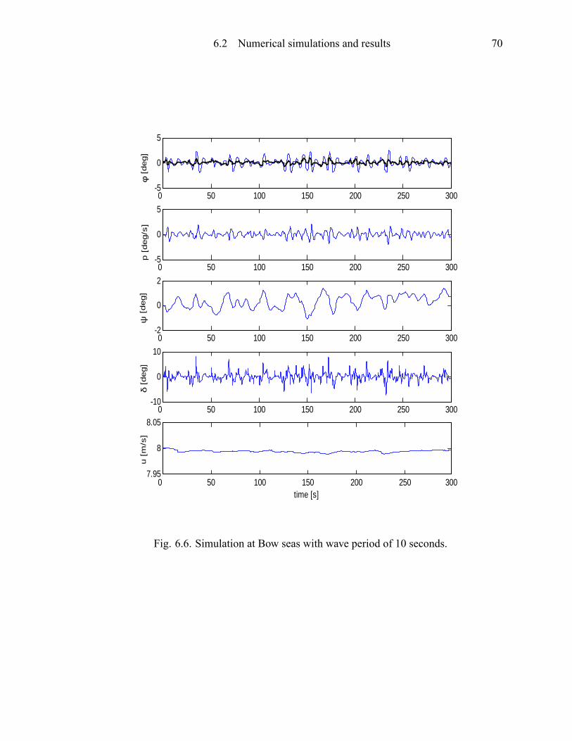
6.2 Numerical simulations and results 70
0 50 100 150 200 250 3005
0
5φ
[deg]
0 50 100 150 200 250 3005
0
5
p [
deg/s
]
0 50 100 150 200 250 3002
0
2
ψ [
deg]
0 50 100 150 200 250 30010
0
10
δ [
deg]
0 50 100 150 200 250 3007.95
8
8.05
time [s]
u [
m/s
]
Fig. 6.6. Simulation at Bow seas with wave period of 10 seconds.

6.3 Double notch sensitivity speci�cation 71
The roll reduction ratio for wave periods from 3 to19 seconds has been calculatedfor this sensitivity based approach controller. The graph illustrating the obtained results isdepicted in Fig. 6.7.
4 6 8 10 12 14 16 18 200.2
0.4
0.6
0.8
1
wave period [sec]
roll
angl
e re
duct
ion
Fig. 6.7. Single notch sensitivity based approach roll reduction ratio as function of waveperiod.
6.3 Double notch sensitivity speci�cationAlthough the method taken in account seemed extremely satisfying and the results obtainedby its implementation were quite successful a discussion needs to be made. Due to theever changing sea state conditions, more detailed research on on-line estimation of thedominating encounter wave frequency is required and the center frequency of the notch�lter should be adjusted accordingly to make the proposed controller adaptive to differentsea states. If a confused sea state is encountered; namely, no dominant frequency existsat all, then the RRS would be of little use and should be turned off. This is because theroll reduction achieved by using the latter controller was effective especially around thenotch frequency. The roll motion was optimally damped in presence of a given sailingcondition but when the encounter frequency moved too much from this original frequency

6.3 Double notch sensitivity speci�cation 72
the performance of the controller was not as satisfying. An alternative solution is thenneeded.
To try to solve this problem a different sensitivity function has been de�ned for thedesign of the controller. This time the output sensitivity function So has been selected as adouble notch �lter in order to obtain a roll reduction for a wider frequency range.
So(s) =(s2 + 2��!ns+ !2n) (s
2 + 2��!n1s+ !2n1)
(s+ !n)2(s+ !n1)2(6.12)
Fig. 6.8 shows the desired shape of the output sensitivity function. Since a broader dampingarea is now desired, as a drawback an inevitably higher ampli�cation for other frequencieswill have to be accepted. The trade off imposed by the non minimum phase zero doesnot allow different solutions. For this reason it is intuitive that in order to have a smallampli�cation at other frequencies a roll damping as good as the single notch speci�cationcan not be expected.
The two frequencies have been selected not to far from one another in order to have asmoother behavior of the controller. It has to be kept in mind that it is not possible to chosefrequencies to close to the right half plane zero because it would in�uence the functioningof the controller and generate a bigger gain for low frequencies. The damping coef�cientas well can not be selected extremely small, so an attentively considered choice has to bemade in setting the right value for �� for both frequencies.
Bode Diagram
Frequency (rad/sec)
102
101
100
101
102
0,2
0,5
1
2
4
ω [rad/s]
|So(j ω
)|
Fig. 6.8. Double notch sensitivity speci�cation.

6.4 Numerical simulations and results 73
The controller C (s) has been based on the process model approximation ~G' (s) thathas been found by multiplying the rudder to roll transfer function by the all pass �lter
(s+ q)
(s� q)(6.13)
Once again the resulting expression for the controller is de�ned using the following nota-tion
C (s) =
�1
S0 (s)� 1�� ~G�1' (s) (6.14)
derived from the de�nition of the sensitivity function expressed as
So (s) =1
1 + C (s) ~G' (s)(6.15)
By substituting the double notch speci�cation in the expression of the controller 6.14 itbecomes
C (s) =(s+ !n)
2(s+ !n1)2 � (s2 + 2��!ns+ !2n) (s
2 + 2��!n1s+ !2n1)
(s2 + 2��!ns+ !2n) (s2 + 2��!n1s+ !2n1)
� ~G�1' (s)(6.16)
and expanding it with respect to the system transfer function given in Eq. 2.11 the controllercan be expressed as:
C (s) =2(1� ��) (!n + !n1) s
3 + 4(1� ��2) (!n!n1) s2 + 2(1� ��) (!2n!n1 + !n!
2n1) s
(s2 + 2��!ns+ !2n) (s2 + 2��1!n1s+ !2n1)
�(p1 + s)(p2 + s)(s2 + 2�!rolls+ !2roll)
Kroll(q + s)(q1 + s)(6.17)
However, since the transfer function 6.17 becomes improper it needs to be modi�ed intro-ducing, as in the latter case, the design parameter, r: The controller can be computed andimplemented with a bi-proper and stable transfer function of the seventh order given by:
C (s) =2(1� ��) (!n + !n1) s
3 + 4(1� ��2) (!n!n1) s2 + 2(1� ��) (!2n!n1 + !n!
2n1) s
(s2 + 2��!ns+ !2n) (s2 + 2��1!n1s+ !2n1)
�(p1 + s)(p2 + s)(s2 + 2�!rolls+ !2roll)
Kroll(q + s)(q1 + s) (s+ r)(6.18)
6.4 Numerical simulations and resultsThe design parameters that determine the characteristics of the output sensitivity functionsde�ned by Eq. 6.12 are selected as follows: the two centered frequencies !n = 0:6, !n1= 1:4; the damping coef�cient �� = 0:65 and r = 3. The corresponding expression for the

6.4 Numerical simulations and results 74
controller C(s) de�ned by Eq. 6.18 is given by
C (s) =�31:6003s(s+ 0:4387)(s+ 0:04306)(s2 + 1:386s+ 0:84)(s2 + 0:1945s+ 1:074)
(s+ 0:3493)(s+ 0:1808)(s+ 3)(s2 + 0:78s+ 0:36)(s2 + 1:82s+ 1:96)(6.19)
while the output sensitivity function is the following
So (s) =(s+ 0:1808)(s+ 3)(s2 + 0:78s+ 0:36)(s2 + 1:82s+ 1:96)
(s2 + 0:2758s+ 0:05559)(s2 + 1:554s+ 0:8397)(s2 + 3:951s+ 8:197)(6.20)
The Bode plot of the obtained roll sensitivity function So(s) is depicted in Fig. 6.9. It canbe seen that the center peak of the sensitivity function is located around 1 rad=sec.
102
101
100
101
102
0,2
0,5
1
2
4
ω [rad/s]
|So(j ω
)|
Bode Diagram
Frequency (rad/sec)
Fig. 6.9. Bode plot of the output sensitivity function for the double notch speci�cation.
From Fig. 6.9 it is clear that an attenuation on roll motion is obtained by this con-troller in the range of wave disturbance. A small roll ampli�cation (around 1.3) exists forsome frequencies, but it has already been said that the values of power spectral densityare very small in such lower ranges of frequencies. Therefore since the disturbance forceand moment are small in those ranges, the small ampli�cation brings no problem for rolldamping performance. The controller is used in simulation to test the performance of theclosed loop system. Simulation conditions and parameters are the same as for the formercontroller. The simulation results are shown in Tables 6.4, 6.5 and 6.6. The maximum roll

6.4 Numerical simulations and results 75
reduction is 56% in RMS value and 81% RSR value. A lower reduction was expected butas it can be gathered there is an increase in the roll damping for disturbances with a higheror lower frequency. A minimum RMS value of 32% has been calculated for Quarteringseas.
Encounter angle for T = 6s !e RMS RSRQuartering sea 0.415rad/s 34% 56%Beam sea 1.047rad/s 56% 81%Bow Sea 1.679rad/s 43% 68%Head Sea 1.941rad/s 33% 56%
Table 6.4. Double notch sensitivity approach controller performances for a 6 seconds pe-riod wave disturbance
Encounter angle for T = 8s !e RMS RSRQuartering sea 0.429 rad/s 36% 59%Beam sea 0.785rad/s 55% 80%Bow Sea 1.141rad/s 55% 80%Head Sea 1.288rad/s 54% 79%
Table 6.5. Double notch sensitivity approach controller performances for a 8 seconds pe-riod wave disturbance
Encounter angle for T = 10s !e RMS RSRQuartering sea 0.407rad/s 32% 54%Beam sea 0.628rad/s 52% 76%Bow Sea 0.856rad/s 55% 80%Head Sea 0.950rad/s 56% 81%
Table 6.6. Double notch sensitivity approach controller performances for a 10 secondsperiod wave disturbance
To show the more effective performance of the system for frequencies far from thecenter notch Fig. 6.10 displays the functioning of the controller for a wave period of 8seconds in Quartering seas. The respective encounter frequency is around 0.4 rad/s. Figure6.12 depicts the behavior for a 6 seconds period wave at Head seas corresponding to afrequency of almost 2 rad/s while in Fig. 6.11 the simulation for a 10 seconds period waveat Beam seas is plotted. In all the situations discussed the rudder angle always respectsits magnitude and velocity limitations. Especially for low frequencies there is a biggerdeviation of the yaw angle while for high frequencies there is almost no deviance at all.The speed of the ship is slightly changed.

6.4 Numerical simulations and results 76
0 50 100 150 200 250 3004
0
4φ
[deg
]
0 50 100 150 200 250 3002
0
2
p [d
eg/s
]
0 50 100 150 200 250 3005
0
5
ψ [d
eg]
0 50 100 150 200 250 30010
0
10
δ [d
eg]
0 50 100 150 200 250 3007.95
8
8.05
time [s]
u [m
/s]
Fig. 6.10. Simulation at Quartering seas with wave period of 8 seconds.

6.4 Numerical simulations and results 77
0 50 100 150 200 250 3005
0
5φ
[deg
]
0 50 100 150 200 250 3002
0
2
p [d
eg/s
]
0 50 100 150 200 250 3002
0
2
ψ [d
eg]
0 50 100 150 200 250 30010
0
10
δ [d
eg]
0 50 100 150 200 250 3007.95
8
8.05
time [s]
u [m
/s]
Fig. 6.11. Simulation at Beam seas with wave period of 10 seconds.

6.4 Numerical simulations and results 78
0 50 100 150 200 250 3005
0
5φ
[deg
]
0 50 100 150 200 250 3005
0
5
p [d
eg/s
]
0 50 100 150 200 250 3005
0
5
ψ [d
eg]
0 50 100 150 200 250 30020
0
20
δ [d
eg]
0 50 100 150 200 250 3007.9
8
8.1
time [s]
u [m
/s]
Fig. 6.12. Simulation at Head seas with wave period of 6 seconds.

6.5 Sensitivity based approach controller robustness 79
The roll reduction ratio for wave periods from 3 to19 seconds has been calculatedfor this second sensitivity based approach controller. The graph illustrating the obtainedresults is depicted in Fig. 6.13. From this plot it can be gathered that the maximum rollreduction is lower than the former studied controllers. However for slow or fast waveperiods, meaning respectively low and high frequencies, the damping achieved is larger.This is due to the different sensitivity speci�cation which aimed in a roll reduction for awider range of frequencies.
4 6 8 10 12 14 16 18 200.2
0.4
0.6
0.8
1
wave period [sec]
roll
angl
e re
duct
ion
Fig. 6.13. Double notch sensitivity based approach roll reduction ratio as function of waveperiod.
6.5 Sensitivity based approach controller robustnessThe results evinced in this chapter demonstrate that for this particular system good perfor-mances are achieved. As in the case of the cheap controller it is interesting to see how thisnominal model used for the design is able to cope with small differences and changes fromthat speci�c representation. The �rst change in the system is made on the constant speedof the ship �u. It has been varied from 6 m/s (yellow line) to 10 m/s (black line) and thereduction ratio for the roll angle for different wave periods has been calculated.

6.5 Sensitivity based approach controller robustness 80
4 6 8 10 12 14 16 18 200.2
0.4
0.6
0.8
1
wave period [sec]
roll
angl
e re
duct
ion
Fig. 6.14. Sensitivity based approach controller roll reduction ratio varying the ship speed.
4 6 8 10 12 14 16 18 200.2
0.4
0.6
0.8
1
wave period [sec]
roll
angl
e re
duct
ion
Fig. 6.15. Sensitivity based approach controller roll reduction ratio varying the roll damp-ing coef�cient

6.5 Sensitivity based approach controller robustness 81
The different results have been plotted in Fig. 6.14. Ship speed variation changesroll angle damping from 0.34 to 0.47 or a factor 1.38 over the parameter envelope for a 8seconds wave. The faster the ship travels the higher effect the rudder induced moment hason the roll diminution. The system has still good results for a small decrease of the constantspeed. However if the speed increases the damping performance remains quite the samefor medium high frequencies and it gets even worse for low frequencies.
The second change has been made varying the value of Kp the roll moment inducedby the roll rate. Its alteration in�uences the roll damping coef�cient and consequently theroll moment induced by the rudder. The roll moment coef�cient has been made differ in arange from �0:1 � 106 (black) to �1:3 � 106 (yellow) Nm=rad=s corresponding to naturaldamping ratios �' from 0.015 to 0.198 as it was in chapter 5. As expected, roll damping ishigher when natural roll damping is small. Roll angle damping for a 8 second wave variesfrom 0.35 to 0.40 or a factor 1.15 as it can be spotted in Fig. 6.15.
4 6 8 10 12 14 16 18 200.2
0.4
0.6
0.8
1
wave period [sec]
roll
angl
e re
duct
ion
Fig. 6.16. Sensitivity based approach controller roll reduction ratio varying �.
The third and �nal change has been made on the damping coef�cient � of the linear�lter H (s) which has been varied from 0.15 (black line) to 0.35 (yellow line). Once againthe reduction ratio for the roll angle for different wave periods has been calculated and theresults have been plotted in Fig. 6.16. When the damping coef�cient is small, meaninga smaller shaping �lter, then the roll damping obtained is higher. This is due to the factthat the wave disturbance is easier to attenuate because its spectrum is concentrated in a

6.5 Sensitivity based approach controller robustness 82
narrower frequency range. The variation of � results in a roll angle damping range between0.32 to 0.40 or a factor 1.26 over the parameter envelope for a 8 seconds wave.
It can be noticed that this controller is less sensitive to small changes in the sys-tem and in the wave disturbances than the minimum variance controller discussed in theprevious Chapter.

Chapter 7Conclusions
A practical and challenging problem considered in this thesis is to realize roll damp-ing by only means of the rudder. In this work, the necessity and the commonly usedschemes of roll damping are discussed. The recent development of rudder roll dampingin Europe and abroad are surveyed, and research that has been done is pointed out. Theeffect of roll on ship performance is discussed and methods used to assess such perfor-mance revised. Two kinds of controller design methods have been discussed. They are theminimum variance cheap control and the sensitivity function-based approach control.
Derivation of a ship mathematical model was done and the model was simpli�edfrom nonlinear to linear so that it could be used in analysis of the characteristics of theclosed loop and in the design of the controller. A model has been created where the inputand output variables were respectively the actual rudder angle and the roll angle of the ship.Wave is a main reason causing the ship to roll. Different wave models have been describedand the relationship between wave and ship roll is discussed. Since the wave disturbanceis treated as a stochastic process it seemed an interesting idea to design a controller thatminimized the output variance of the system. Using the Youla parametrization the �rstrudder roll damping controller has been implemented.
The second approach consisted in directly shaping the output sensitivity function.Thanks to the fact that it depends linearly on the system transfer function the expressionof the controller is derived. Two different speci�cations have been given: a single notchwith a higher damping and a narrower frequencies range, and a double notch with a lowerdamping but a wider range.
The simulations in a sea-way have been made with these controllers for the model ofthe ship. Different sailing conditions and frequency of encounter were considered. Whenthe three controllers designed were applied to the ship model, the cheap controller hadthe best roll reduction performance. The double notch had the worst maximum dampingperformance but had the best results for low and high frequencies. The performance inroll reduction of the single notch controller was in the middle between the former twocontrollers.
Robustness properties of rudder-roll-damping control have been treated. An investi-gation was made on the effects of changes in the ship speed and in the roll damping coef-�cient given by the shape of the rudder. The controllers performance has been tested withdifferent wave spectra obtained by changing the shaping �lter damping coef�cient �:It wasshown that small changes in some parameters can result in important changes to the controldynamics, and in the performance of the control system. The minimum variance controllerwas found to be more sensitive to these small variations in the system characteristics thanthe sensitivity based approach controller.
83

7.1 Future work 84
7.1 Future workDifferent aspects of this thesis call for further investigation and future development. Therudder can be used for heading control and roll reduction at the same time. An interestingcontinuing of this thesis could lead to the design of a control system incorporating bothautopilot and rudder roll stabilizer. However simultaneous control is not a simple task. Thekey issue would be the study of the difference in dynamic response between roll and yawcharacterized by the location of the Non-minimum phase zero.
An appealing possibility could be a research of the effects of uncertainty on the Rud-der roll damping controller using and changing the data from the naval multipurpose vesselemployed in this thesis.
Last different controllers design including the combined use of the rudder and otherroll stabilizer devices such as �ns or bilge keels can be applied in order to enhance the rollreduction performance.

References
[1] E. Baitis, D.A. Woolaver and T.A. Beck. Ship Roll Stabilization in The U. S. Navy,Naval Engineers Journal, Vol. 101 pp.43-53, 1989.
[2] M. Blanke, Uncertainty Models for Rudder-Roll Damping Control, Proc. of The13thWorld Congress of IFAC, Vol.Q, pp. 285-290, San Francisco, USA, 1996.
[3] M. Blanke and A. C. Christensen, Rudder-Roll Damping Autopilot Robustness to Sway-Yaw-Roll Couplings, Proc. of The 10th International Ship Control Systems Symposium(SCSS'93),Vol.A, pp.93-119, Ottawa, Canada, 1993.
[4] M. Blanke, P. Haals and K.K. Andreasen, Rudder Roll Damping Experience in Den-mark, Proc. of IFAC Workshop on Expert Systems and Signal Processing in MarineAutomation CAMS, pp.149-160, Lyngby, Denmark 1989.
[5] M. Blanke, M. Kinnaert, J. Lunze and M. Staroswiecki, Diagnosis and Fault-TolerantControl, 2nd Edition, Springer, 2006.
[6] W.E. Cowley and T.H. Lambert, The Use of Rudder as a Roll Stabilizer, 3rd ShipControl System Symposium-SCSS, Bath, UK, 1972.
[7] O. M. Faltinsen, Sea Loadson Shipsand Offshore Structures, Cambridge UniversityPress, 1990.
[8] K. K. Fedyaevsky and G.V. Sobolev, Control and Stability in Ship Design, State UnionShipbuilding, Leningrad, 1963.
[9] Thor I. Fossen, Marine Control Systems. Guidance Navigation, and Control of Ships,Rigs and Underwater Vehicles. Marine Cybernetics, 2002.
[10] W. Froude, The papers of William Froude chapter On the Rolling of Ships, The Insti-tution of Naval Architects, pp 40-65, 1995.
[11] C. G. Goodwin, S. Graebe and M. Salgado, Control system Design, Prentice Hall 2001.
[12] S. Haverre and T. Moan, On some uncertainties related to short term stochastic mod-elling of ocean waves. In: Probabilistic Offshore Mechanics, Progress in EngineeringScience, CML Publications Ltd, 1985.
85

References 86
[13] G. Hearns and M. Blanke, Quantitative Analysys and Design of Rudder Roll DampingController. In Proc. of CAMS, 1998.
[14] A. Isidori, Non Linear Control Systems, Springer, 3rd Edition, 1995.
[15] C.G. Källström, P. Wessel and S. Sjolander, Roll Reduction by Rudder Control, Proc.of SNAME Spring Meeting/STAR Symposium, pp. 67-76, Pittsburg, Pennsylvania,USA.1988.
[16] C.G. Källström andW.L. Schultz, An Integrated Rudder Control System for Roll Damp-ing and Maintenance, Proc. of The 9th International Ship Control Systems Symposium,pp. 3.278-3.296, Bethesda, MD, 1990.
[17] T. Laudval and T. I. Fossen, Rudder Roll Stabilization for Ships subject to input ratesaturation using sliding mode control, Proc. of IFAC CAMS'98, pp 121-126,1998.
[18] T. Lauvdal and T.. I. Fossen, Nonlinear Rudder Roll Damping of Non-minimum PhaseShips using Sliding Mode Control, Proc. of the European Control Conference, Brussel,Belgium, 1997.
[19] Norwegian University of Science and Technology. ntnu-mss, marine system simulator.www.cesos.ntnu.no/mss, 2007.
[20] N. H. Norrbin, Theory of Observations on the Use of a Mathematical Model for ShipManeuvering in Deep and Con�ned Water, 8th Symposium on Naval Hydrodynamics,USA, 1970.
[21] Norwegian University of Science and Technology NTNU, Department of Marine Tech-nology, Marine Control Systems.
[22] T. Perez, Ship Motion Control. Course Keeping and Roll Stabilization Using Rudderand Fins. Springer, 2005.
[23] T. Perez and M. Blanke, Simulation of Ship Motion in Seaway, Technical ReportEE02037, 2002.
[24] S. Skogestad and I. Postlethwaite, Multivariable Feedback Control. Analysis and De-sign, John Wiley & Sons, Ltd 2005.
[25] K. H. Son and K. Nomoto, On The Coupled Motion of Steering and Rolling of A HighSpeed Container Ship, Journal of Naval Architecture and Ocean Engineering, Vol.20,pp.73-83, 1982.

References 87
[26] R. Taggart, Anomalous Behavior of Merchant Ship Steering Systems, Marine Technol-ogy, April pp 205-215, 1970.
[27] Ching-Yaw Tzeng, Chung-Yi Wu and Yu-Lung Chu, A Sensitivity Function Approachto the Design of Rudder Roll Stabilization Controller, Journal of Marine Science andTechnology, Vol. 9, No. 2, pp. 100-112, 2001.
[28] J. van Amerongen, P.G.M. van der Klugt and H.R. van Nauta Lemke, Rudder RollStabilization for Ships, Automatica, Vol. 26, pp 679-690, 1990.
[29] P.G.M. Van der Klugt, Rudder Roll Stabilization, Ph.D. Thesis, Delft University ofTechnology, The Netherlands, 1987.
[30] F.F. van Gunsteren, Analysis of Roll Stabilizer Performance, Trans. of The Society ofNaval Architects and Marine Engineers SNAME, Vol. 69 pp 411-439, 1961.
[31] L.F. Whicker and L.F. Fehlner, Free-stream Characteristics of a Family of Low-aspectRatio Control Surfaces for Application to Ship Design, Report 933, DTRC, 1958.
[32] Cheng'en Yang, Robust Rudder Roll Damping Control, Ph.D. Thesis, Marine Engi-neering Institute of Dalian Maritime University , 1998.
[33] Cheng'en Yang and Mogens Blanke, A Robust Roll Damping Controller, Proc. of The4th IFAC Conf. on Manoeuvring and Control of Marine Craft MCMC, pp.60-64, Bri-juni, Croatia, 1997.

Appendix ANaval vessel data
A.1 Principal multipurpose naval vessel data
Table A.1. Main data for multipurpose naval vessel used in the project and for the simula-tion.
Main particulars Value and unitLength between perpendiculars Lpp 51.5 mBeam B 8.6 mDraft D 2.55 mMass m 359.77�103 KgDisplacement r 351�103 m3
Inertia in yaw Izz 47.934�106 Kg�m2
Inertia in roll Ixx 23.763�106 Kg�m2
Nominal speed U 8 ktLateral Centre of Gravity LCG 23.5 mVertical Centre of Gravity VCG 3.36 mTransverse Metacentric Height GMt 0.97 mRudder Area Ar 2 m2
Rudder Span sp 2 mMean cord c̄ 1 mLift coef�cient CL 3.09Stall angle �stall 23 degDistance from propeller lprop 1.5 mSea water density � 1025 Kg/m3
Gravity constant g 9.81 m/s2
88

A.2 Manoevering coef�cients 89
A.2 Manoevering coef�cients
Table A.2. hydrodynamic parameters for multipurpose vessel used in the project and forthe simulation.
X-coef�cients Y-coef�cients K-coef�cients N-coef�cientsX _u = �17400 Y _v = �393000 K _v = 296000 N _v = 538000Xujuj = �1960 Y _p = �296000 K _p = �774000 N _p = 0Xvr = 0:33 �m Y _r = �1400000 K _r = 0 N _r = �40:744 � 106
Yjujv =-11800 Kjujv = 9260 Njujv = �92000Yur = 131000 Kur = �102000 Nur = �4710000Yvjvj = �37400 Kvjvj = 29300 Nvjvj = 0Yrjrj = 0 Krjrj = 0 Nrjrj = �20:2 � 106Yvjrj = �794000 Kvjrj = 621000 Nvjrj = 0Yrjvj = �182000 Krjvj = 142000 Nrjvj = �15:6 � 106Y'juvj = 10800 K'juvj = �8400 N'juvj = �214000Y'jurj = 251000 K'jurj = �196000 N'ujrj = �4980000Y'uu = �74 K'uu = �1180 N'ujuj = �8000Yjujp = 0 Kjujp = �15500 Njujp = 0Ypjpj = 0 Kpjpj = �416000 Npjpj = 0Yp = 0 Kp = �500000 Np = 0Y' = 0 K''' = �0:325 �m � g N' = 0Y''' = 0 N''' = 0