ship structure committee 2011 structure committee 2011 ship structure committee radm p.f. zukunft u....
TRANSCRIPT

NTIS # PB2011-
SSC-459
RELIABILITY-BASED
PERFORMANCE ASSESSMENT OF DAMAGED SHIPS
This document has been approved For public release and sale; its
Distribution is unlimited
SHIP STRUCTURE COMMITTEE 2011

Ship Structure Committee RADM P.F. Zukunft
U. S. Coast Guard Assistant Commandant, Assistant Commandant for Marine Safety, Security
and Stewardship Co-Chair, Ship Structure Committee
RDML Thomas Eccles Chief Engineer and Deputy Commander For Naval Systems Engineering (SEA05)
Co-Chair, Ship Structure Committee
Mr. H. Paul Cojeen
Society of Naval Architects and Marine Engineers Dr. Roger Basu
Senior Vice President American Bureau of Shipping
Mr. Christopher McMahon
Director, Office of Ship Construction Maritime Administration
Mr. Victor Santos Pedro Director Design, Equipment and Boating Safety,
Marine Safety, Transport Canada
Mr. Kevin Baetsen
Director of Engineering Military Sealift Command
Dr. Neil Pegg Group Leader - Structural Mechanics
Defence Research & Development Canada - Atlantic
Mr. Jeffrey Lantz, Commercial Regulations and Standards for the
Assistant Commandant for Marine Safety, Security and Stewardship Mr. Jeffery Orner
Deputy Assistant Commandant for Engineering and Logistics
Mr. Edward Godfrey Director, Structural Integrity and Performance Division
Dr. John Pazik
Director, Ship Systems and Engineering Research Division
SHIP STRUCTURE SUB-COMMITTEE
AMERICAN BUREAU OF SHIPPING (ABS) DEFENCE RESEARCH & DEVELOPMENT CANADA
ATLANTIC Mr. Craig Bone Mr. Phil Rynn
Mr. Tom Ingram
Dr. David Stredulinsky Mr. John Porter
MARITIME ADMINISTRATION (MARAD) MILITARY SEALIFT COMMAND (MSC) Mr. Chao Lin
Mr. Richard Sonnenschein Mr. Michael W. Touma
Mr. Jitesh Kerai
NAVY/ONR / NAVSEA/ NSWCCD TRANSPORT CANADA Mr. David Qualley / Dr. Paul Hess
Mr. Erik Rasmussen / Dr. Roshdy Barsoum Mr. Nat Nappi, Jr.
Mr. Malcolm Witford
Natasa Kozarski Luc Tremblay
UNITED STATES COAST GUARD SOCIETY OF NAVAL ARCHITECTS AND MARINE
ENGINEERS (SNAME) CAPT John Nadeau CAPT Paul Roden Mr. Jaideep Sirkar Mr. Chris Cleary
Mr. Rick Ashcroft Mr. Dave Helgerson Mr. Alex Landsburg Mr. Paul H. Miller


CONVERSION FACTORS
(Approximate conversions to metric measures) To convert from to Function Value
LENGTH inches meters divide 39.3701 inches millimeters multiply by 25.4000 feet meters divide by 3.2808 VOLUME cubic feet cubic meters divide by 35.3149 cubic inches cubic meters divide by 61,024 SECTION MODULUS inches2 feet2 centimeters2 meters2 multiply by 1.9665 inches2 feet2 centimeters3 multiply by 196.6448 inches4 centimeters3 multiply by 16.3871 MOMENT OF INERTIA inches2 feet2 centimeters2 meters divide by 1.6684 inches2 feet2 centimeters4 multiply by 5993.73 inches4 centimeters4 multiply by 41.623 FORCE OR MASS long tons tonne multiply by 1.0160 long tons kilograms multiply by 1016.047 pounds tonnes divide by 2204.62 pounds kilograms divide by 2.2046 pounds Newtons multiply by 4.4482 PRESSURE OR STRESS pounds/inch2 Newtons/meter2 (Pascals) multiply by 6894.757 kilo pounds/inch2 mega Newtons/meter2
(mega Pascals) multiply by 6.8947
BENDING OR TORQUE foot tons meter tons divide by 3.2291 foot pounds kilogram meters divide by 7.23285 foot pounds Newton meters multiply by 1.35582 ENERGY foot pounds Joules multiply by 1.355826 STRESS INTENSITY kilo pound/inch2 inch½(ksi√in) mega Newton MNm3/2 multiply by 1.0998 J-INTEGRAL kilo pound/inch Joules/mm2 multiply by 0.1753 kilo pound/inch kilo Joules/m2 multiply by 175.3

CONTENTS
Section Title Page 1 Introduction 11.1 Background 11.2 Objectives and Scope of Work 42 Methodologies 72.1 Methodologies for Wave-Induced Loading 72.1.1 Linear two-dimensional strip theory 72.1.2 Nonlinear time-domain method 92.1.3 Responses under irregular waves 122.1.4 Experimental investigation 132.1.5 Model uncertainties of numerical methods 152.2 Methodologies for Combining Different Loads 172.3 Methodologies for Assessing Ultimate Strength of Hull Girders 192.3.1 Reliability based assessment of damaged ship residual strength 213. A Sample Vessel, Its Model and Damage Scenarios 273.1 Descriptions of the Sample Vessel and Its Model 273.2 Damage Scenarios 324. Measurement and Analysis of Loads 394.1 Introduction 394.2 Predictions of Global Dynamic Wave-Induced Loads using 2-D Linear
Method 40
4.2.1 Effects of transverse location of gravity centre 404.2.2 Results in intact condition 434.2.3 Results in damage scenario 2 564.2.4 Results in damage scenario 3 724.2.5 Nonlinearity of the wave-induced dynamic loads 814.3 Prediction of Dynamic Global Wave Loads using 2-D Nonlinear Theory 954.4 Model Uncertainties of 2-D Linear and Nonlinear Method 1155. Prediction of Extreme Design Loads and Load Combinations 1215.1 Prediction of extreme design loads using the results from the 2-D linear
method 121
5.2 Prediction of extreme design loads using the results from the 2-D nonlinear method
130
5.3 Load combinations for strength assessment 1346. Ultimate Strength of Hull Girders 1396.1 Hull 5415 and Damaged Scenario 1396.2 Ultimate Hull Girder Strength – using MARS 1416.3 Ultimate Hull Girder Strength – using ANSYS 1536.3.1 Finite element model for nonlinear ultimate strength assessment 1546.3.2 Initial deformations 1586.3.3 Material model 1606.3.4 Load modelling and boundary conditions 1606.3.5 FE analysis results and discussion 161
iv

CONTENTS
Section Title Page 7. Reliability based assessment of intact and damaged structure 1738. Summary 1779. Conclusions 18310. Recommendations 184 Acknowledgement 18511. References 185App. A RAOs of Wave-induced Loads of the Sample Vessel 191App. B Model Uncertainties of the 2-D Linear Method 201App. C Model Uncertainties of the 2-D Nonlinear Method 239App. D The Rule-based Formulae for predicting Extreme Design Loads 249
v

List of Figures
Figure Title Page 2.1-1 Co-ordinate systems and modes of motions 72.1-2 Co-ordinate systems (Chan et al, 2003) 92.1-3 Test arrangement 112.3-1 Reliability analysis using FE analysis response surface 232.3-2 Damaged ship structure, variables relevant for reliability based assessment
of residual structural strength. 24
2.3-3 Number of random variables and computational effort 253-1 Division of the compartments of the vessel 283-2 The ship model (Lee, et al 2006) 293-3: Weight distribution of the intact sample vessel 293-4 Weight distribution of the intact model 293-5 Model compartmentation for damage containment 303-6 General view of the model for loading tests in damaged conditions 313-7 The cling film in the NICOP project 313-8 The cling film in the current project 32
Damage scenario 1 333-9 Damage scenario 2 343-10 Damage scenario 3 353-11
4.2.1-1 Torsion moment RAO in intact condition in stern quartering waves 414.2.1-2 Torsion moment RAO in intact condition in bow quartering waves 414.2.1-3 Torsion moment RAO in DS 2 in stern quartering waves (heading 45) 424.2.1-4 Torsion moment RAO in DS 2 in stern quartering waves (heading 315) 424.2.1-5 Torsion moment RAO in DS 3 in stern quartering waves 434.2.2-1 Horizontal shear force RAO in intact condition in head waves 464.2.2-2 Vertical shear force RAO in intact condition in head waves 474.2.2-3 Torsion moment RAO in intact condition in head waves 474.2.2-4 Vertical bending moment RAO in intact condition in head waves 484.2.2-5 Horizontal bending moment RAO in intact condition in head waves 484.2.2-6 Horizontal shear force in intact condition in stern quartering waves 494.2.2-7 Vertical shear force RAO of intact condition in stern quartering waves 494.2.2-8 Torsion moment RAO in intact condition in stern quartering waves 504.2.2-9 Vertical bending moment RAO in intact condition in stern quartering waves 504.2.2-10 Horizontal bending moment RAO in intact condition in stern quartering
waves 51
4.2.2-11 Horizontal shear force RAO in intact condition in bow quartering waves 514.2.2-12 Vertical shear force RAO in intact condition in bow quartering waves 524.2.2-13 Torsion moment RAO in intact condition in bow quartering waves 524.2.2-14 Vertical bending moment RAO in intact condition in bow quartering waves 534.2.2-15 Horizontal bending moment RAO in intact condition in bow quartering
waves 53
4.2.2-16 Horizontal shear force RAO in intact condition in beam waves 544.2.2-17 Vertical shear force RAO in intact condition in beam waves 54
vi
List of Figures Title Page Figure
4.2.2-18 Torsion moment RAO in intact condition in beam waves 554.2.2-19 Vertical bending moment RAO in intact condition in beam waves 554.2.2-20 Horizontal bending moment RAO in intact condition in beam waves 564.2.3-1 Horizontal shear force RAO in DS 2 in head waves 584.2.3-2 Vertical shear force RAO in DS 2 in head waves 584.2.3-3 Torsion moment RAO in DS 2 in head waves 594.2.3-4 Vertical bending moment RAO in DS 2 in head waves 594.2.3-5 Horizontal bending moment RAO in DS 2 in head waves 604.2.3-6 Horizontal shear force RAO in DS 2 in stern quartering waves 604.2.3-7 Vertical shear force RAO in DS 2 in stern quartering waves 614.2.3-8 Torsion moment RAO in DS 2 in stern quartering waves 614.2.3-9 Vertical bending moment RAO in DS 2 in stern quartering waves 624.2.3-10 Horizontal bending moment RAO in DS 2 in stern quartering waves 624.2.3-11 Horizontal shear force RAO in DS 2 in stern quartering waves (heading
315) 63
4.2.3-12 Vertical shear force RAO in DS 2 in stern quartering waves (heading 315) 634.2.3-13 Torsion moment RAO in DS 2 in stern quartering waves (heading 315) 644.2.3-14 Vertical bending moment RAO in DS 2 in stern quartering waves (heading
315) 64
4.2.3-15 Horizontal bending moment RAO in DS 2 in stern quartering waves (heading 315)
65
4.2.3-16 Horizontal shear force RAO in DS 2 in beam waves (heading 90) 654.2.3-17 Vertical shear force RAO in DS 2 in beam waves (heading 90) 664.2.3-18 Torsion moment RAO in DS 2 in beam waves (heading 90) 664.2.3-19 Vertical bending moment RAO in DS 2 in beam waves (heading 90) 674.2.3-20 Horizontal bending moment RAO in DS 2 in beam waves (heading 90) 674.2.3-21 Horizontal shear force RAO in DS 2 in beam waves (heading 270) 684.2.3-22 Vertical shear force RAO in DS 2 in beam waves (heading 270) 684.2.3-23 Torsion moment RAO in DS 2 in beam waves (heading 270) 694.2.3-24 Vertical bending moment RAO in DS 2 in beam waves (heading 270) 694.2.3-25 Horizontal bending moment RAO in DS 2 in beam waves (heading 270) 704.2.3-26 Comparison of vertical bending moment between different wave angles in
stern quartering seas 70
4.2.3-27 Comparison of horizontal bending moment between different wave angles in stern quartering seas
71
4.2.3-28 Comparison of horizontal bending moment between different wave angles in beam seas
71
4.2.3-29 Comparison of torsion moment between different wave angles in stern quartering seas
72
4.2.4-1 Horizontal shear force RAO in DS 3 in head waves 734.2.4-2 Vertical shear force RAO in DS 3 in head waves 744.2.4-3 Torsion moment RAO in DS 3 in head waves 744.2.4-4 Vertical bending moment RAO in DS 3 in head waves 75
vii

List of Figures Title Page Figure
4.2.4-5 Horizontal bending moment RAO in DS 3 in head waves 754.2.4-6 Horizontal shear force RAO in DS 3 in stern quartering waves 764.2.4-7 Vertical shear force RAO in DS 3 in stern quartering waves 764.2.4-8 Torsion moment RAO in DS 3 in stern quartering waves 774.2.4-9 Vertical bending moment RAO in DS 3 in stern quartering waves 774.2.4-10 Horizontal bending moment RAO in DS 3 in stern quartering waves 784.2.4-11 Horizontal shear force RAO in DS 3 in beam waves 784.2.4-12 Vertical shear force RAO in DS 3 in beam waves 794.2.4-13 Torsion moment RAO in DS 3 in beam waves 79
Vertical bending moment RAO in DS 3 in beam waves 804.2.4-14 4.2.4-15 Horizontal bending moment RAO in DS 3 in beam waves 804.2.5-1 Horizontal shear force RAO in stern quartering waves 814.2.5-2 Vertical shear force RAO in stern quartering waves 824.2.5-3 Torsion moment RAO in stern quartering waves 824.2.5-4 Vertical bending moment RAO in stern quartering waves 834.2.5-5 Horizontal bending moment RAO in stern quartering waves 834.2.5-6 Horizontal shear force RAO in bow quartering waves 844.2.5-7 Vertical shear force RAO in bow quartering waves 844.2.5-8 Torsion moment RAO in bow quartering waves 854.2.5-9 Vertical bending moment RAO in bow quartering waves 854.2.5-10 Horizontal bending moment RAO in bow quartering waves 864.2.5-11 Horizontal shear force RAO in stern quartering waves (heading 45) 864.2.5-12 Vertical shear force RAO in stern quartering waves (heading 45) 874.2.5-13 Torsion RAO in stern quartering waves (heading 45) 874.2.5-14 Vertical bending moment RAO in stern quartering waves (heading 45) 884.2.5-15 Horizontal bending moment RAO in stern quartering waves (heading 45) 884.2.5-16 Horizontal shear force RAO in stern quartering waves (heading 315) 894.2.5-17 Vertical shear force RAO in stern quartering waves (heading 315) 894.2.5-18 Torsion moment RAO in stern quartering waves (heading 315) 904.2.5-19 Vertical bending moment RAO in stern quartering waves (heading 315) 904.2.5-20 Horizontal bending moment RAO in stern quartering waves (heading 315) 914.2.5-21 Horizontal shear force RAO in stern quartering waves 914.2.5-22 Vertical shear force RAO in stern quartering waves 924.2.5-23 Torsion moment RAO in stern quartering waves 924.2.5-24 Vertical bending moment RAO in stern quartering waves 934.2.5-25 Horizontal bending moment RAO in stern quartering waves 934.2.5-26 Vertical shear force RAO in head waves 944.2.5-27 Vertical bending moment RAO of in head waves 94
Dynamic vertical shear force RAO in head seas (heading 180), theory ζ = 2m
984.3-1
4.3-2 Dynamic vertical shear force RAO in head seas (heading 180), theory ζ = 2.5m
99
viii

List of Figures Title Page Figure
Dynamic vertical bending moment RAO in head seas (heading 180), theory ζ = 2m
994.3-3
4.3-4 Dynamic vertical bending moment RAO in head seas (heading 180), theory ζ = 2.5m
100
4.3-5 Dynamic horizontal shear force RAO in stern quartering seas (heading 45), theory ζ = 2m
100
4.3-6 Dynamic horizontal shear force RAO in stern quartering seas (heading 45), theory ζ = 2.5m
101
4.3-7 Dynamic vertical shear force RAO in stern quartering seas (heading 45), theory ζ = 2m
101
4.3-8 Dynamic vertical shear force RAO in stern quartering seas (heading 45), theory ζ = 2.5m
102
4.3-9 Dynamic vertical bending moment RAO in stern quartering seas (heading 45), theory ζ = 2m
102
4.3-10 Dynamic vertical bending moment RAO in stern quartering seas (heading 45), theory ζ = 2.5m
103
4.3-11 Dynamic horizontal bending moment RAO in stern quartering seas (heading 45), theory ζ = 2m
103
4.3-12 Dynamic horizontal bending moment RAO in stern quartering seas (heading 45), theory ζ = 2.5m
104
4.3-13 Dynamic torsion moment RAO in stern quartering seas (heading 45), theory ζ = 2m
104
4.3-14 Dynamic torsion moment RAO in stern quartering seas (heading 45), theory ζ = 2.5m
105
4.3-15 Dynamic horizontal shear force RAO in head seas (heading 180), theory ζ = 2m
105
4.3-16 Dynamic horizontal shear force RAO in head seas (heading 180), theory ζ = 2.5m
106
Dynamic vertical shear force RAO in head seas (heading 180), theory ζ = 2m
1064.3-17
4.3-18 Dynamic vertical shear force RAO in head seas (heading 180), theory ζ = 2.5m
107
4.3-19 Dynamic vertical bending moment RAO in head seas (heading 180), theory ζ = 2m
107
4.3-20 Dynamic vertical bending moment RAO in head seas (heading 180), theory ζ = 2.5m
108
Dynamic horizontal bending moment RAO in head seas (heading 180), theory ζ = 2m
1084.3-21
4.3-22 Dynamic horizontal bending moment RAO in head seas (heading 180), theory ζ = 2.5m
109
ix

List of Figures Title Page Figure
4.3-23 Dynamic torsion moment RAO in head seas (heading 180), theory ζ = 2m 109Dynamic torsion moment RAO in head seas (heading 180), theory ζ =
2.5m 1104.3-24
4.3-25 Dynamic horizontal shear force RAO in stern quartering seas (heading 45), theory ζ = 2m
110
4.3-26 Dynamic horizontal shear force RAO in stern quartering seas (heading 45), theory ζ = 2.5
111
4.3-27 Dynamic vertical shear force RAO in stern quartering seas (heading 45), theory ζ = 2m
111
4.3-28 Dynamic vertical shear force RAO in stern quartering seas (heading 45), theory ζ = 2.5m
112
4.3-29 Dynamic vertical bending moment RAO in stern quartering seas (heading 45), theory ζ = 2m
112
4.3-30 Dynamic vertical bending moment RAO in stern quartering seas (heading 45), theory ζ = 2.5m
113
4.3-31 Dynamic horizontal bending moment RAO in stern quartering seas (heading 45), theory ζ = 2m
113
4.3-32 Dynamic horizontal bending moment RAO in stern quartering seas (heading 45), theory ζ = 2.5m
114
4.3-33 Dynamic torsion moment RAO in stern quartering seas (heading 45), theory ζ = 2m
114
4.3-34 Dynamic torsion moment RAO in stern quartering seas (heading 45), theory ζ = 2.5m
115
5.1-1 Location of Sea Area 16 1226.1-1 Midship scantling of Hull 5415 1406.2-1 Midship section, MARS model intact ship 1446.2-2 Midship section, MARS model damaged condition 1446.2-3 Elastic – Ideally Plastic ultimate strength of Hull 5415 in pure horizontal
bending. 145
6.2-4 Beam-Column failure mode ultimate strength of Hull 5415 in pure vertical bending
146
6.2-5 EIP ultimate strength of Hull 5415 for vertical and horizontal moments 1476.2-6 EIP ultimate strength for vertical and horizontal moments interaction 1476.2-7 BC ultimate strength of Hull 5415 for vertical and horizontal moments 1486.2-8 BC ultimate strength of Hull 5415 for vertical and horizontal interaction 148
Comparison of Mv/Muv and Mh/Muh for intact and damaged conditions 1496.2-9 6.2-10 Ultimate hogging moment for intact and damaged conditions 1496.2-11 Comparison of ultimate moment for intact and damaged sagging conditions 1506.2-12 Percentage reduction in ultimate hogging and sagging moment for intact
and damaged conditions 150
6.2-13 Ultimate sagging moment as function of damaged depth 151
x
List of Figures Title Page Figure
6.2-14 Ultimate hogging moment as a function of damaged depth 1516.2-15 Ultimate horizontal bending moment as a function of damaged depth 1526.2-16 Shift in vertical location of neutral axis as a function of damaged depth 1526.2-17 Inclination angle of neutral axis as a function of damaged depth 1536.3-1 The range of ship for FE modelling of damaged ship analysis 1546.3.1-1 Different model for FE Analysis. 1566.3.1-2 Damaged structural model ANSYS/LS DYNA simulation 1566.3.1-3 Residual stress in the damaged part of model structure 1576.3.1-4 Refined mesh of damaged structure 1586.3.2-1 Initial deformation model for FE analysis 1596.3.2-2 Initial deformation as applied to mid part of 3-compartment model. 1606.3.4-1 Applied pure vertical bending moment equivalent force on section 1616.3.5-1 Ultimate vertical moment capacity of the 1-compartment model 1646.3.5-2 Horizontal ultimate moment capacity of the 1-compartment model 1656.3.5-3 Horizontal ultimate moment capacity of 2 frame model 1666.3.5-4 Deformation and stress distribution of damaged 3-compartment. model 1676.3.5-5 Ultimate torsion – 3-compartment FE analysis 1686.3.5-6 Ultimate torsion – 2 frame FE mode 1686.3.5-7 Mv and Mh interaction – 2-frame FE analysis results 1696.3.5-8 Comparison of MARS results with 2-frame FE analysis results 1696.3.5-9 Comparison of ultimate moment, MARS and 2-frame FE results 1706.3.5-10 Ultimate moment, percentage difference between MARS and FE results 1706.3.5-11 Interaction response surface for Mv, Mh and Mt moment; FE results 1717-1 The reliability index for different sea state – damaged case 175
List of Tables
Table Title Page 2.1-1 Test Conditions of the First Batch of Wave-induced Loads Tests 152.1-2 Definitions of Different Categories of Wave Heights in Table 2.1-1 152.3-1 LR Rules; collision damage extent 253-1 Main particulars of Hull 5415 and its model 273-2 Intact and damage conditions of the design ship 363-3 Intact stability and trim summary of the design ship 363-4 Intact and damage conditions of the ship model 373-5 Intact stability and trim summary of ship model 38
Model uncertainties of the 2-D linear method )X( 1m 1164.4-1 4.4-2 Model uncertainties of the 2-D nonlinear method )X( 1m 1195.1-1 Annual sea state occurrences in the North Atlantic and North Pacific 1215.1-2 Wave scatter diagram of sea area 16 in the North Atlantic 1225.1-3 Extreme design loads in stern quartering waves (heading 45) 123
xi

List of Tables
Table Title Page 5.1-4 Extreme design loads in head waves (heading 180) 1245.1-5 Extreme design loads in beam waves (heading 90) 1245.1-6 Extreme design loads in stern quartering waves (heading 45) 1255.1-7 Extreme design loads in head waves (heading 180) 1255.1-8 Extreme design loads in beam waves 1265.1-9 Extreme design loads in stern quartering waves (heading 45) 1265.1-10 Extreme design loads in head waves 1275.1-11 Extreme design loads in beam waves (heading 90) 1275.1-12 Extreme design loads beam waves (heading 270) 1285.1-13 Extreme design loads in stern quartering waves (heading 315) 1285.1-14 Extreme design loads in stern quartering waves (heading 45) 295.1-15 Extreme design loads in head waves 1295.1-16 Extreme design loads in beam waves 1305.2-1 Extreme design loads by the 2-D nonlinear method in intact condition 1315.2-2 Extreme design loads by the 2-D nonlinear method in DS 2 1325.2-3 Extreme vertical bending moment in intact condition 1335.2-4 Extreme vertical bending moment in DS 2 1335.3-1 Load combinations in intact condition at 45 heading 1355.3-2 Load combinations in damage scenario 1 at 45 heading 1356.1-1 Principal dimension of USN Hull 5415 1396.1-2 Properties of steel materials 1396.1-3 Cross section characteristics 1416.1-4 Section modulus required as per BV Rules and actual for the midship
section 141
Statistics of yield strength, σy, of steel materials (MN/m2) 1606.3.3-1 6.3.5-1 Comparison of ultimate vertical bending moment from different methods 1716.3.5-2 Comparison of ultimate strength of intact and damaged ship 1727-1 Reliability analysis results 174
xii

EXECUTIVE SUMMARY When a ship is damaged, the operators need to decide the immediate repair actions by evaluating the effects of the damage on the safety of the ship using residual strength assessment procedure. The objective of this project is to develop a procedure and tools for operators and decision makers to assess the residual ultimate hull girder strength of damaged ships for a given damage scenario. This study is a continuation of NICOP project (Lee, et al 2006), in which an assessment procedure was developed. In order for the readers to understand the significance of the current project, the assessment procedure is briefly described here. This procedure consists of four steps: (1) Identify the location and size of the openings; (2) Calculate the still water bending moment and wave-induced loadings including vertical bending moment, horizontal bending moment and torsion; (3) Calculate the ultimate hull girder strength of the damaged cross-section considering the interaction of vertical bending moment, horizontal bending moment and torsion; (4) Assess the structural integrity by deterministic and probabilistic approaches. In Step 1, once a ship is damaged, the location and size in terms of length, height and depth of the penetration of the opening should be determined, so the degree of water ingress could be predicted. In Step 2, the floating conditions of the ship need to be calculated. The stillwater bending moment and wave-induced loads are then estimated. Because it is desirable to install the developed tools on board of ships for a quick and reliable assessment, computational time is a very important factor in choosing a particular method for both loading calculations and strength assessment. In Step 3, the ultimate hull girder strength of the damaged cross-section needs to be assessed. The interaction of vertical bending moment, horizontal bending moment and torsion should be considered. In addition, the strength of other cross-sections (not the damaged one), where the total load including stillwater bending moment and wave-induced loads under the damage conditions exceed that in intact condition, should also be assessed. In Step 4, reliability of the damaged ship is calculated so a well-informed decision could be made based on this information. In the current project, some tools for predicting wave-induced loads and assessing ultimate hull girder strength have been further developed. In particular, a 2-D linear and a nonlinear method have been applied to the ship model to calculate the wave-induced loads in regular waves at the cut where the force gauge is installed to measure the loads in the experimental tests. The numerical results have been compared with the experimental results. The 2-D linear method was shown to predict accurately wave-induced vertical bending moments in head seas and stern quartering seas, but the accuracy deteriorates with increases in wave amplitude. The accuracy in predicting horizontal bending moment is not as good as that for vertical bending moment, but is acceptable in most cases. However, the predictions of torsion moment are not satisfactory, although the magnitude of the torsion moments were low and did not affect the results of the study. The experimental results have revealed that majority of the response RAOs show a nonlinear trend in which the non-dimensional responses are decreasing as wave amplitude increases in most frequency ranges, especially at the frequency where the responses achieve the maximum. For vertical bending moment this trend is very remarkable. It may be said that the high nonlinearity is an inherent feature of the sample vessel with a very fine hull form.
xiii

Because the damage on the ship is unsymmetrical transversely, it is expected that the wave-induced loads might be different when the wave is approaching the ship model from different sides due to the dynamic behaviour of the flooded water in the damaged compartment. The test results have shown that the vertical bending moment at 45° wave heading at most of frequencies was slightly larger than that at 315° wave heading. There was no clear trend for horizontal bending moment at 45° and 315° wave headings. However, the horizontal bending moment in beam seas at 90° wave headings is slightly larger than that at 270° wave headings. The torsion moment at 315° wave headings is larger than that in 45° wave headings. The 2-D nonlinear method does not produce satisfactory results for vertical bending moment, horizontal bending moment and torsion moment in regular waves. Although this conclusion was largely based on the analysis of the results in 2-metre wave height, it was equally applicable to the results in 2.5-metre wave height. Again the predictions of torsion moment are the worst among the three components of the wave-induced loads, while the predictions of vertical bending moment have similar level of accuracy to those of horizontal bending moment. The nonlinear method tends to produce better results at the resonant frequencies than at the other frequencies. However it should be pointed out that the measured wave heights were not equal to 2.0 metres, which was used in the numerical calculations, at most frequencies. Model uncertainties of both 2-D linear and nonlinear methods have been calculated. For the 2-D linear method, it is observed that the accuracy, which is measured by the mean and COV of the model uncertainty factor, of vertical bending moment is generally better than that of horizontal bending moment and torsion moment, and the accuracy for loads in head seas is much better than those in stern quartering seas and beam seas. This could be mainly caused by the underwater hull form of the ship model with a small Cb compared with conventional ships. The COV of horizontal bending moment is almost as twice as that of vertical bending moment. The COV of torsion moment is the largest of the three. Because of the large difference in COV for different force components it is more rational to consider the model uncertainties for vertical bending moment, horizontal bending moment and torsion moment separately in reliability analysis rather than using one combined model uncertainty for all the components. It can be seen that the 2-D linear method has better mean and COV of Xm in the predictions of vertical bending moment and horizontal bending moment in both intact condition and damage scenario 2 than the 2-D nonlinear method, and both 2-D linear and nonlinear methods have produced unsatisfactory results in torsion moment. Based on the current results, it may be said that the 2-D linear method is more accurate than the nonlinear method. However the nonlinear method can distinguish the difference between the positive and negative responses, but linear methods can’t. This advantage of the nonlinear method is especially important for ships with small block coefficient, such as frigates, etc. For a frigate the ratio of sagging bending moment to hogging bending moment could be as large as 1.78 (Clarke, 1986). In addition, hull girder strength in hogging is normally different from that in sagging. Therefore the nonlinear method is preferred. This slight preference of the nonlinear method was also based on another fact that the nonlinear method tends to produce better results in the resonant region than at other frequencies. Based on the current method for combining different load components, the accuracy in resonant region is more important than that at other frequencies.
xiv
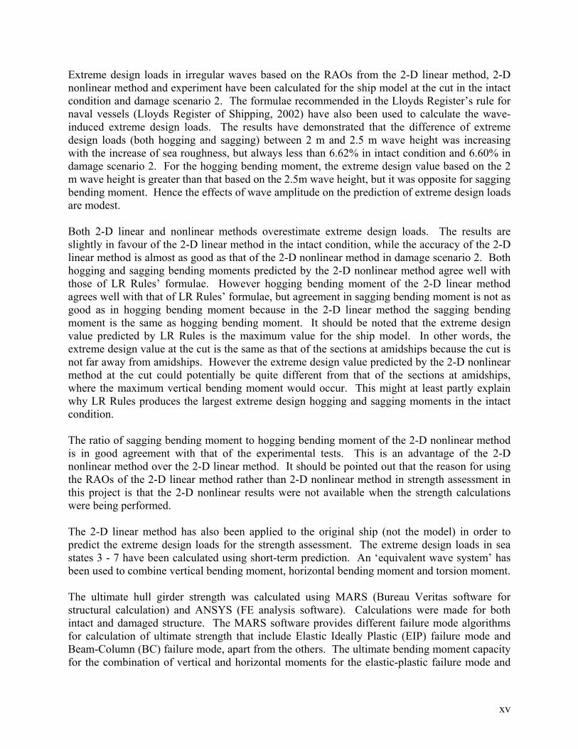
Extreme design loads in irregular waves based on the RAOs from the 2-D linear method, 2-D nonlinear method and experiment have been calculated for the ship model at the cut in the intact condition and damage scenario 2. The formulae recommended in the Lloyds Register’s rule for naval vessels (Lloyds Register of Shipping, 2002) have also been used to calculate the wave-induced extreme design loads. The results have demonstrated that the difference of extreme design loads (both hogging and sagging) between 2 m and 2.5 m wave height was increasing with the increase of sea roughness, but always less than 6.62% in intact condition and 6.60% in damage scenario 2. For the hogging bending moment, the extreme design value based on the 2 m wave height is greater than that based on the 2.5m wave height, but it was opposite for sagging bending moment. Hence the effects of wave amplitude on the prediction of extreme design loads are modest. Both 2-D linear and nonlinear methods overestimate extreme design loads. The results are slightly in favour of the 2-D linear method in the intact condition, while the accuracy of the 2-D linear method is almost as good as that of the 2-D nonlinear method in damage scenario 2. Both hogging and sagging bending moments predicted by the 2-D nonlinear method agree well with those of LR Rules’ formulae. However hogging bending moment of the 2-D linear method agrees well with that of LR Rules’ formulae, but agreement in sagging bending moment is not as good as in hogging bending moment because in the 2-D linear method the sagging bending moment is the same as hogging bending moment. It should be noted that the extreme design value predicted by LR Rules is the maximum value for the ship model. In other words, the extreme design value at the cut is the same as that of the sections at amidships because the cut is not far away from amidships. However the extreme design value predicted by the 2-D nonlinear method at the cut could potentially be quite different from that of the sections at amidships, where the maximum vertical bending moment would occur. This might at least partly explain why LR Rules produces the largest extreme design hogging and sagging moments in the intact condition. The ratio of sagging bending moment to hogging bending moment of the 2-D nonlinear method is in good agreement with that of the experimental tests. This is an advantage of the 2-D nonlinear method over the 2-D linear method. It should be pointed out that the reason for using the RAOs of the 2-D linear method rather than 2-D nonlinear method in strength assessment in this project is that the 2-D nonlinear results were not available when the strength calculations were being performed. The 2-D linear method has also been applied to the original ship (not the model) in order to predict the extreme design loads for the strength assessment. The extreme design loads in sea states 3 - 7 have been calculated using short-term prediction. An ‘equivalent wave system’ has been used to combine vertical bending moment, horizontal bending moment and torsion moment. The ultimate hull girder strength was calculated using MARS (Bureau Veritas software for structural calculation) and ANSYS (FE analysis software). Calculations were made for both intact and damaged structure. The MARS software provides different failure mode algorithms for calculation of ultimate strength that include Elastic Ideally Plastic (EIP) failure mode and Beam-Column (BC) failure mode, apart from the others. The ultimate bending moment capacity for the combination of vertical and horizontal moments for the elastic-plastic failure mode and
xv

xvi
for the beam-column method were found and interaction formulae were derived based on that. It may be observed that for the hogging condition when the bending curvature ratio (ratio of horizontal to vertical moments) is small and, consequently, predominant curvature is in the vertical direction depicting a predominant vertical bending moment, the difference between ultimate moments for damaged and intact conditions is small. The finite element analysis was carried out using ANSYS, since no FE based design assessment of the intact ship was available to compare the results with that of the damaged ship. The FE analysis for ultimate strength of the hull girder was carried out for both intact and damaged conditions. Two types of moment interaction functions were developed, one set of two combinations of moments such as interaction of vertical and horizontal moments, and one set for interaction of all the moments viz. vertical, horizontal and torsion moment. The vertical and horizontal moment interaction function obtained from FE analysis was compared with that of the MARS beam-column and elastic-plastic interaction diagram. The ultimate moment estimates obtained using beam-column method is higher than that from the two-frame finite element analysis. The difference between the two results diminishes as the Mv/Mh moment ratio increases. The reliability analysis was carried out using CALREL software, the First Order Reliability Method (FORM) and Monte Carlo Simulation (MCS). The results from the finite element analysis were used for deriving the limit state function. The reliability-based assessment of hull structure was made for both intact and damaged condition. The reliability assessment for intact condition is made for the worse case scenario, Sea State 7 and for lesser sea states. Three combinations of loads identified from the ship loading analysis were included in the calculations.
1. INTRODUCTION
1.1 Background
A large number of ship accidents continue to occur despite advances in navigation systems. These accidents have caused the loss of cargos, pollution of the environment, and loss of human lives. Based on statistical data from Lloyd’s Register of Shipping (Lloyd’s Register, 2000), a total of 1,336 ships were lost with 6.6 million gross tonnage cargo losses between 1995 and 2000. 2,727 people were reported killed or missing as a result of total losses in this period. A survey of the accidents of Greek ships over 100 GRT from 1993 to 2002 has revealed that about 48 percent of the losses were caused by grounding, collision, and excessive loading (Samuelides, et al., 2007). Therefore it is very important to ensure an acceptable safety level for damaged ships. Unfortunately adequate structural strength in the intact condition does not necessarily guarantee an acceptable safety margin in damaged conditions. In conventional design practice only the structural strength in the intact condition is assessed.
Recognising the importance of the residual strength of ships, the International Maritime Organisation (IMO) has proposed an amendment, which states: ‘All oil tankers of 5,000 tonnes deadweight or more shall have prompt access to computerised, shore-based damage stability and residual structural strength calculation programmes.’
When a ship is damaged, the operators need to decide the immediate repair actions by evaluating the effects of the damage on the safety of the ship using a residual strength assessment procedure. Various publications have investigated, as summarised in the following, the local and overall structural behaviour of a damaged ship. Smith and Dow (1981) carried out pioneer work in assessing residual strength of damaged ships and offshore structures. Strength reduction of dented stiffened panels was investigated. The effect of this reduction on the ultimate strength of hull girder was further assessed.
Qi, et al. (1999) derived a simplified method for assessing the residual strength of hull girders of damaged ships. Reliability of the ship was also estimated by a first order and second moment method.
Wang, et al. (2002) have tried to use the section modulus to indicate the residual strength of damaged ships. Both section modulus and ultimate strength of damaged ships were calculated. A regression analysis was carried out to derive an empirical formula for predicting safety level of damaged ships.
A few more papers (Ghoneim and Tadros, 1992, Paik, 1992, Paik, et al., 1995, Zhang, et al., 1996, Paik, et al., 1998, Ghose, et al., 1995) have discussed the residual strength of damaged ships from different viewpoints.
All the above work only studied the ultimate vertical bending moment capacity without considering the effect of the horizontal bending moment and torsion and the critical load case was not evaluated. This means that the worst load case was assumed to be the vertical bending moment, and the horizontal bending moment and torsion are negligible. This methodology was, strictly
1

speaking, only valid for ships in the intact condition. In the design of ships, structural strength is conventionally assessed only in the intact condition. Under this condition, the critical load case for a mono-hull ship is the vertical bending moment, which reaches maximum in head seas. Both horizontal bending moments and torsion are considered to be insignificant. Torsion is considered only when there are large openings on ships. This methodology has been successfully applied to ship design for many years. Because of this, the prediction of environmental loads and assessment of structural strength were normally carried out separately by two groups of people. When the ultimate strength of the hull girder is assessed, only vertical bending moment is considered. Although some researchers have tried to evaluate the effect of horizontal bending moments and shear on the ultimate strength (Paik, et al., 1996), it is concluded that these effects are insignificant. But this conclusion is only valid for the intact condition.
When a ship is in a damaged condition its floating condition could be changed dramatically. Its draught is increased and it may heel. It could also have large holes in the structure. If the methodology used for intact conditions is blindly applied to damaged conditions, the results could be misleading. Ideally the environmental loads should be calculated together with the assessment of the residual strength of the ship. In another words, a systematic approach should be used for a more accurate assessment of residual strength of a damaged ship. Chan, et al., (2001) have shown that the most critical condition for a damaged Ro-Ro ship is in quartering seas. Although the vertical bending moment in quartering seas is smaller than that in head seas, the horizontal bending moment is quite large. The ratio of horizontal bending moment to vertical bending moment could be as large as 1.73, so the combined effect of vertical bending moment and horizontal bending moment is more serious. In addition, torsion, which was not considered in the above study, normally reaches the maximum in quartering seas, so the effect of horizontal bending moment and torsion on the ultimate hull girder strength should be considered in the assessment of residual strength of damaged ships.
From 2004 to 2006 the Office of Naval Research (USA) sponsored a project, NICOP, which shares the same title as the current project, Reliability-Based Performance Assessment of Damaged Ships, to address some of the important issues associated with damaged ships (Lee, et al., 2006). The participants include Y.W. Lee, Y. Pu, H.S. Chan, A. Incecik and R.S. Dow in Newcastle University, I. Khan and P.K. Das in the University of Glasgow and Strathclyde, and P.E. Hess in the Naval Surface Warfare Center Carderock Division (NSWCCD) in the USA. In that study, a procedure was developed to assess the structural integrity of damaged ships. The procedure consists of four steps: (1) Identify the location and size of the openings; (2) Calculate the still water bending moment and wave-induced loadings including vertical bending moment, horizontal bending moment and torsion; (3) Calculate the ultimate hull girder strength of the damaged cross-section considering the interaction of vertical bending moment, horizontal bending moment and torsion; (4) Assess the structural integrity by deterministic and probabilistic approaches. The state of the art of the methods for predicting environmental loads and assessing the structural safety was reviewed. The developed procedure was applied to a sample vessel, HULL 5415, to demonstrate the applicability of the proposed procedure.
The hydrodynamic loads in regular waves were calculated in that project using a 2-D linear
2
method. Experimental tests on a ship model with a scale of 1/100 were also been carried out to predict the hydrodynamic loads in regular waves. The results of the theoretical method and experimental tests were compared to validate the theoretical method and to calculate the modelling uncertainties of the theoretical method for probabilistic strength assessment. The comparison of theoretical results with experimental results has revealed that the prediction of vertical bending moment of the 2-D linear method agrees reasonably well with the experimental results, while the prediction of horizontal bending moment is acceptable. However the accuracy of the torsion moment was generally poor. Further research is required to improve the accuracy in this area.
The extreme wave-induced loads have been calculated by short-term and long-term predictions. For the loads in the intact condition, long-term prediction with a duration of 20 years was used, while for loads in damaged conditions short-term predictions were used. The maximum values of the most probable extreme amplitudes of dynamic wave induced loads in damaged conditions are much less than those in intact condition, because the most probable extreme load in intact condition is based on long term prediction, while the most probable extreme load for damaged conditions is based on short term prediction under sea state 3 for 96 hours, as recommended by Lloyds Register in their rules for naval ships (Lloyds, 2002).
An opening could change the distribution of not only the stillwater bending moment but also the wave-induced bending moment. It is observed that although some cross sections are not structurally damaged, the total loads (including stillwater bending moment and wave-induced bending moment) acting on these cross sections after damage (in other locations) may be increased dramatically compared to the original design load in the intact condition. In this case the strength of these cross sections also needs to be assessed.
The ultimate strength of the hull 5415 was predicted using progressive analysis, the results of which compare well with those of another program developed by Bureau Veritas (BV). Although the strength assessment of all the critical cross sections should be carried out in practice, not all the cross sections have structural details for this hypothetical vessel. Therefore only those critical cross sections with structural details available were assessed to demonstrate the applicability of the developed methods.
The residual strength in four different damage scenarios was compared. In damage scenarios 1 and 2, where the locations of the damage is near the elastic neutral axis, the residual strength has been about 96.6 percent and 93 percent of the ultimate strength in the hogging condition. Similarly the residual strength for damage scenarios 3 and 4 shows significant decrease compared to the ultimate strength.
Deterministic strength assessment of the damaged ships was carried out by considering the interaction of vertical and horizontal bending moments for the intact condition in damage scenario 2. It was found that the damaged ship is quite safe with a fairly high safety margin. This is due to the relatively small wave-induced loads, which were based on a short-term prediction, and at the same time the extent of damage was fairly moderate, and did not reduce the ultimate strength too much. The residual strength has also been assessed by a probabilistic approach. The limit state
3
function used for reliability analysis was derived from an interaction equation including vertical and horizontal bending moments, which was developed in the deterministic strength assessment. The reliability index for HULL 5415 in intact condition was calculated. Overall, the developed procedure and the methods worked well, but the NICOP study revealed the need for further research in some areas. That need is addressed in the project being reported, which extended the previous work in the following areas:
• A different method of sealing the midship joint in the model was used in the testing programme to increase the accuracy of the results, particularly the torsion moments.
• The hydrodynamic analysis was extended to use a nonlinear 2-D method to predict wave-induced loads.
• The strength of the hull was evaluated using finite element modelling. • The reliability analysis was extended to include survival in higher sea states, up to
Sea State 7.
1.2 Objectives and Scope of Work
The objective of this project is to develop a procedure and tools for operators and decision makers to assess the residual ultimate hull girder strength of damaged ships for a given damage scenario. To achieve this objective, the following work packages were addressed:
• Develop a method for predicting wave-induced loading on damaged ships, and validate the method by comparing with experimental results so that its model uncertainty could be determined.
• Develop the damaged ship structural strength predictions with a focus on hull girder bending using numerical analysis.
• Develop reliability-based analysis procedure for determining the recoverability and operability of damaged ships.
This project is a continued effort of the NICOP project discussed above (Lee et al., 2006). While these two projects share the same objectives, the current project focused on the following tasks: Task 1: Apply the 2-D linear method to predict wave-induced loads on the ship model. In this task, an in-house program, which is based on a 2-D linear theory (Chan, 1992), was chosen to predict wave-induced loads in regular waves. This method is capable of dealing with unsymmetrical floating conditions, which is a unique feature of damaged ships. The program is also capable of modelling flooding in compartments. The details of this method are described in Section 2.1.1, while the results are presented in Section 4.2. Task 2: Apply the 2-D nonlinear method to predict wave-induced loads on the ship model. In this task, another in-house program, which is based on a 2-D nonlinear method (Chan, et al., 2003), has been used to predict wave-induced loads in regular waves. This method calculates wave-induced loads in the time domain. Unsymmetrical floating conditions and flooding in compartments can also be considered in this method. The details of the method will be described in Section 2.1.2, and the results will be presented in Section 4.3. Task 3: Carry out more experimental tests to validate both the 2-D linear and nonlinear methods.
4

Experiments have been carried out to investigate the structural responses of a ship model with a scale of 1/100. The results revealed important phenomena at various damaged conditions, and were used to validate both the 2-D linear and nonlinear methods. The test facilities and other details of running the tests will be shown in Section 2.1.4, and the results will be presented in Chapter 4.
Task 4: Calculate model uncertainties of both 2-D linear and nonlinear methods for reliability analysis. In this task, model uncertainties of both the 2-D linear and nonlinear methods were calculated. These are important parameters that influence the reliability of strength assessment. The method is presented in Section 2.1.5 and the results are presented in Section 4.4.
Task 5: Calculate extreme design loads in irregular waves using short-term prediction. Extreme design loads in irregular waves have been calculated using short-term prediction for the original sample vessel at amidships. Response Amplitude Operators (RAOs) of the 2-D linear method have been used. These results are used for strength assessment in Task 7. In addition, RAOs from the 2-D linear method, 2-D nonlinear method, and from the experiments have been used to calculate the extreme design load of the ship model at the cut where the force gauge is installed in order to compare the results of the different methods. The formulae recommended by Lloyds Register of Shipping (Lloyds Register of Shipping, 2002) are also used to predict the extreme design loads. The method is presented in Section 2.1.3, and the results are in Chapter 5.
Task 6: Combine different load components, such as vertical bending moment, horizontal bending moment, and torsion, in order to assess structural integrity under combined load conditions. One of the aims of this project is to investigate the effects of horizontal bending moments and torsion on the ultimate hull girder strength of damaged ships. In this task, vertical bending moments, horizontal bending moments, and torsion are combined. These results were developed by the Newcastle University research team and were then passed onto the research team of the University of Glasgow and Strathclyde to assess the strength of the sample vessel. The method is presented in Section 2.2 and the results are in Section 5.3.
Task 7: Develop the damaged ship structural strength predictions with a focus on hull girder bending using numerical analysis. The ultimate hull girder strength of the damaged cross-section was assessed. This task was accomplished using ANSYS finite element analysis software and MARS (Bureau Veritas software for structural calculations). The interaction of vertical bending moments, horizontal bending moments, and torsion were considered. In addition, the strength of other cross-sections than the damaged one, where the total load including the stillwater bending moment and wave-induced loads under the damaged conditions exceed that in intact condition, was assessed. The method and results can be found in Chapter 6.
Task 8: Develop a reliability-based analysis procedure for determining the recoverability and operability of damaged ships. The reliability-based assessment of hull structure was made for both intact and damaged conditions. The reliability assessments for the intact and damaged conditions were made for the worse case scenario, Sea State 7, and for lesser sea states, and included three load combinations as identified from the ship loading analysis. The reliability analysis was carried out using CALREL software to perform analysis using both the First
5

6
Order Reliability Method (FORM) and Monte Carlo Simulation (MCS). The reliability index and relevant probabilities as calculated are given in table 5.6.3.6.1 for both intact and damaged case.
This research has been jointly carried out by Newcastle University and the University of Glasgow and Strathclyde. Tasks 1–6 were executed by Newcastle University, while the others were executed at the University of Glasgow and Strathclyde.
This report consists of ten chapters. Chapter 1 presents the background, objectives and scope of the project. The state of the art of the techniques has been reviewed in the NICOP project (Lee, et al., 2006), so it was only briefly discussed in this report. The details of the methods that are used in this project are presented in Chapter 2. Chapter 3 shows the particulars of the sample vessel and its model, and describes briefly three damage scenarios used in the following calculations. Chapter 4 describes the measurement and analysis of loads, and Chapter 5 presents the prediction of extreme design loads and load combinations. Chapter 6 contains the analyses of the ultimate strength of the hull girder, and the reliability analysis of the intact and damaged ship in various sea states is presented in Chapter 7. The results have been analysed and discussed in Chapter 8, which summarises the major findings of the current project. Finally, recommendations have been made in Chapter 9. The References are contained in Chapter 10.
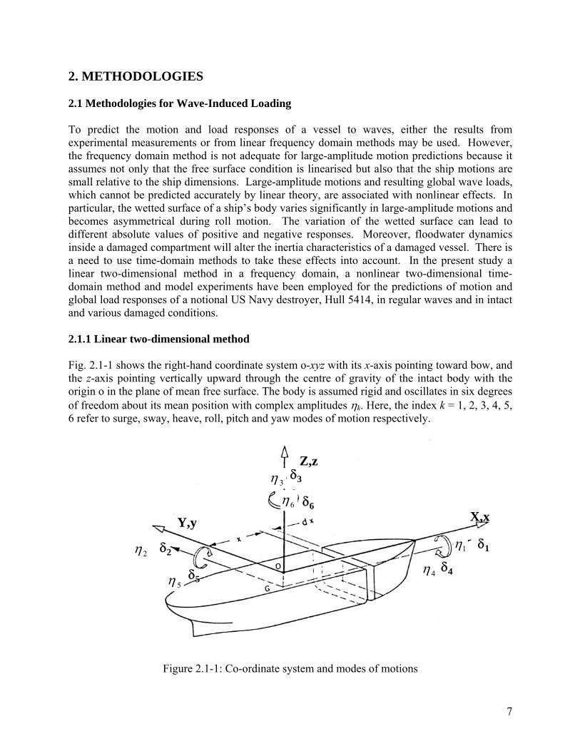
2. METHODOLOGIES 2.1 Methodologies for Wave-Induced Loading To predict the motion and load responses of a vessel to waves, either the results from experimental measurements or from linear frequency domain methods may be used. However, the frequency domain method is not adequate for large-amplitude motion predictions because it assumes not only that the free surface condition is linearised but also that the ship motions are small relative to the ship dimensions. Large-amplitude motions and resulting global wave loads, which cannot be predicted accurately by linear theory, are associated with nonlinear effects. In particular, the wetted surface of a ship’s body varies significantly in large-amplitude motions and becomes asymmetrical during roll motion. The variation of the wetted surface can lead to different absolute values of positive and negative responses. Moreover, floodwater dynamics inside a damaged compartment will alter the inertia characteristics of a damaged vessel. There is a need to use time-domain methods to take these effects into account. In the present study a linear two-dimensional method in a frequency domain, a nonlinear two-dimensional time-domain method and model experiments have been employed for the predictions of motion and global load responses of a notional US Navy destroyer, Hull 5414, in regular waves and in intact and various damaged conditions. 2.1.1 Linear two-dimensional method Fig. 2.1-1 shows the right-hand coordinate system o-xyz with its x-axis pointing toward bow, and the z-axis pointing vertically upward through the centre of gravity of the intact body with the origin o in the plane of mean free surface. The body is assumed rigid and oscillates in six degrees of freedom about its mean position with complex amplitudes ηk. Here, the index k = 1, 2, 3, 4, 5, 6 refer to surge, sway, heave, roll, pitch and yaw modes of motion respectively.
X,x
Z,z
Y,yδ1δ2
δ3
δ4 δ5
δ6
3η
6η
1η2η
4η5η
Figure 2.1-1: Co-ordinate system and modes of motions
7

For dynamic equilibrium the coupled linear equations of motion of the rigid body can be written
as
for j = 1, 2, …6 (2.1-1) jk
kjkkjkkjkjk FCBAM =⋅+⋅+⋅+∑=
6
1])[( ηηη &&&
where kη&& and kη& are motion acceleration and velocity respectively; Mjk is the generalised mass; Ajk is the added mass; Bjk is the damping; Cjk is the restoring coefficients; Fj is the wave exciting force or moment. The indices j and k indicate the direction of force and the mode of motion respectively. The generalised mass matrix [M] of a damaged ship whose centre of gravity is at (xG, yG, zG) is given by
(2.1-2) [ ]
⎥⎥⎥⎥⎥⎥⎥⎥
⎦
⎤
⎢⎢⎢⎢⎢⎢⎢⎢
⎣
⎡
−−−−−−−−−
−−
−
=
666564
565554
464544
00
0000
000000
IIIMxMyIIIMxMzIIIMyMz
MxMyMMxMzMMyMzM
M
GG
GG
GG
GG
GG
GG
in which M is the mass of the ship including floodwater, Ijj is the moment of inertia about the origin in the jth mode of motion and Ijk is the cross-product of inertia about the origin. The added mass, damping coefficients, and wave exciting forces can be calculated by integration of the sectional values over the ship length L, and can be expressed respectively as (2.1-3) ( )∫=
Ljkjk dxxaA
(2.1-4) ( )∫=
Ljkjk dxxbB
(2.1-5) ( )∫=
Ljj dxxfF
where ajk, bjk and fj are respectively the sectional values of added mass, damping coefficient and wave-exciting force. The details of calculations of ajk, bjk and fj can be found in Chan et al. (2002). The global wave-induced loads Pj on a particular transverse cross-section x of the ship body can be expressed as
8
for j = 1, 2, …6 (2.1-6) ( ) ( ) ( ) ( )xFxCxBxAmP jk
kjkkjkkjkjkj −⋅+⋅+⋅+= ∑=
6
1])[( ηηη &&&
where P1, P2 and P3 represent wave-induced longitudinal force, horizontal shear force and vertical shear force respectively, while P4, P5 and P6 are wave-induced torsional moment, vertical bending moment and horizontal bending moment respectively. mjk is generalised mass for the portion aft the cross-section. (2.1-7) ( ) ( )∫=
xjkjk daxA ξξ
(2.1-8) ( ) ( )∫=x
jkjk dbxB ξξ
(2.1-9) ( ) ( )∫=x
jj dfxF ξξ
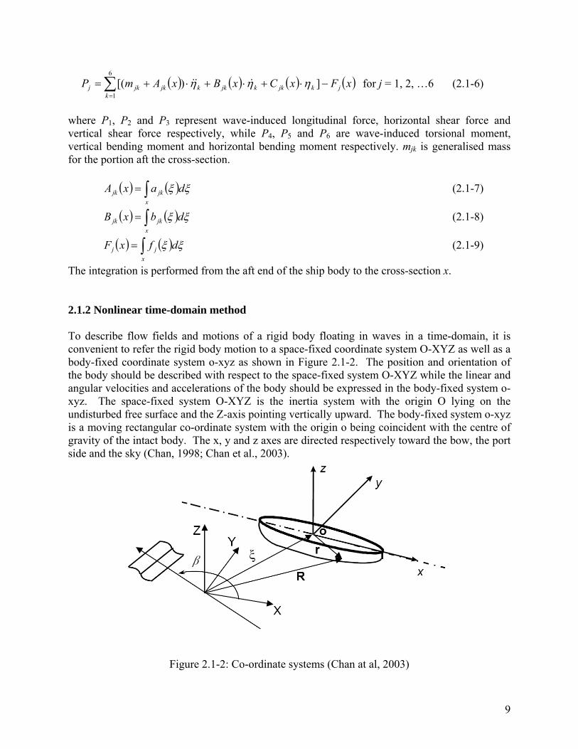
The integration is performed from the aft end of the ship body to the cross-section x. 2.1.2 Nonlinear time-domain method To describe flow fields and motions of a rigid body floating in waves in a time-domain, it is convenient to refer the rigid body motion to a space-fixed coordinate system O-XYZ as well as a body-fixed coordinate system o-xyz as shown in Figure 2.1-2. The position and orientation of the body should be described with respect to the space-fixed system O-XYZ while the linear and angular velocities and accelerations of the body should be expressed in the body-fixed system o-xyz. The space-fixed system O-XYZ is the inertia system with the origin O lying on the undisturbed free surface and the Z-axis pointing vertically upward. The body-fixed system o-xyz is a moving rectangular co-ordinate system with the origin o being coincident with the centre of gravity of the intact body. The x, y and z axes are directed respectively toward the bow, the port side and the sky (Chan, 1998; Chan et al., 2003).
Figure 2.1-2: Co-ordinate systems (Chan at al, 2003)
9

The position and orientation vectors of the body-fixed axes with respect to the space-fixed frame are defined respectively in the form X ),,( 321 ηηη= (2.1-10)
Ω ),,( 654 ηηη= (2.1-11) The relationship between a body-fixed position vector r and a space-fixed position vector R can be written as R = X + T r (2.1-12) where T is an orthogonal transformation matrix (Chan 1998). The Euler equations of motion of a rigid body in six degrees of freedom with respect to the body-fixed co-ordinate system are defined by Chan 1998 as
(2.1-13(2.1-1( ) ( ) 4) )( )& & &m r m rG G Gv + × + + × + × + × × =ω ω ω ω ωv v r F
( )& & & &I r I I rω ω ω ω ω+ × + + × + × + ×m mG Gv v M=vin which m is the body mass; I is the matrix of second moment of inertia; v and ω are linear and angular velocity vectors respectively; the dot stands for time derivative with respect to the body-fixed frame; rG is a position vector of the centre of gravity of the body; F and M are the external force and moment vectors respectively. The body-fixed angular velocity vector ω and the Euler angular velocity vector dΩ/dt can be related through a transformation matrix Γ (Chan 1998). dΩ/dt = Γ ω (2.1-15) Equations (2.1-13) and (2.1-14) represent a set of six second-order ordinary differential equations and can be solved by numerically integration over time using 4th order Runge-Kutta method.
Within the framework of linear potential flow theory the components of the external force F and moment M can be generalised in the form
( ) jjk
jkjkjj WCBAFF −++−= ∑=
6
1jj vv~
& (2.1-16)
where j and k indicate the direction of external force and velocity (acceleration) respectively in the body-fixed co-ordinate system; Fj is the wave exciting force; Ajk is the added mass; Bjk is the damping coefficient; Cj is the buoyancy force; Wj is the force due to gravitation. These hydrodynamic forces due to radiation and wave excitation at each time step can be calculated by
10

integration of sectional values at the incident wave profile. The sectional values of hydrodynamic coefficients and wave exciting forces at various ship sections can be obtained by means of two-dimensional source distribution technique (Kim et al., 1980). The buoyancy force and moment of a submerged body are calculated by integration of the sectional area and moment of the submerged section. The external force F and moment M are time dependent and become nonlinear. The hydrodynamic coefficients are coupled with each other when the ship sections are no longer symmetrical. For a damaged hull loss of buoyancy can be accounted for in the calculations of buoyancy force and moment by means of the lost buoyancy method or added weight method. The linear and nonlinear loads analysis programmes that were used account for damage using the added weight method. In the linear method, the added weight corresponds to the flooding water when the ship is in the stillwater floating position, and in the nonlinear model the added weight changes instantaneously with changes in wave height and ship motion. No compartment permeabilities were used in these calculations. The position vector rG of an intact ship is equal to zero as the origin of the body-fixed system is defined at the centre of gravity of intact ship and the ship mass m and inertia matrix I is constant. The dynamic effects of flooding water in a damaged compartment on ship motion are taken into account by adding the time dependent mass of flooding water into the ship mass m. Consequently the mass m, inertia matrix I and the position vector rG of a damaged ship vary with time. As it is difficult to simulate the free surface of flooding water, the sloshing effects are not considered in the present study. For simplicity the level of flooding water is assumed to be the same height as that of the incident wave profile.
Since the ship body is free to drift, she will inevitably drift away from the nominal heading angle β. In order to maintain the wave-heading angle within a reasonable range, an artificial restoring yaw moment c6 is introduced in the equations of motion and may be expressed by
c a I z z6 = − ζ ωο
2 (2.1-17) where a is a constant; ζ is wave amplitude and Izz is yaw moment of inertia. In the present study the constant a of 0.1 is used outside roll resonant region. In addition to potential roll damping B44, viscous roll damping b44 obtained from roll decay tests is used in the prediction of roll motion the in roll resonant region.
Although the equations of motion are fully nonlinear, the hydrodynamic forces due to incident waves, radiation waves and diffraction waves are still linear and calculated up to the incident wave profile. No radiation and diffraction waves are considered on the free surface. As a consequence, drift motions predicted by the present numerical model may be unrealistic.
After solving the nonlinear Euler equations of motion at each time step, the dynamic global wave loads can be easily calculated. They are expressed by Chan 1998 as
( )(2.1-18)
( )
( )( )∫
∫××+×+×+−
×+−−=
x
xS
dxm
xdmPPP
rr
rFF
ωωωω
ω
vv
v,, 321
&
&
11
( )
( )∫
∫×+×−×−−
×+−×−−=
x
xcS
dxm
dxmPPP
vv
v,, 654
ωωωω
ω
&&
&&
rII
rIPrMM
where the over-bar implies that the integration is carried out from one end to the particular cut. Fs and Ms are shear force and bending moment vectors due to still water loads. rc is the position vector of the point of interest at which the dynamic shear force vector P acts.
(2.1-19) 2.1.3 Responses under irregular waves The elevation of the ocean waves is irregular and has a random nature in a seaway. In practice linear theory is used to simulate irregular seas and to obtain statistical estimates. The wave spectrum can be estimated from wave measurements that were made during a limited time period in the range from ½ hour to around 10 hours. In the literature this is often referred to as a short-term description of the sea. The ITTC spectrum can be used to calculate significant values and other characteristics of wave exciting forces and responses in short term prediction method (Hasselmann at al, 1973; DNV, 2000). In this study short-term prediction was used to predict extreme design loads. In this method, a wave spectrum is chosen to describe the irregular wave condition. The response spectrum )(ωrS can be expressed as: ( ) 2)()( ωωω HSSr = (2.1.20) Where )(ωS is the wave spectrum, )(ωH is the transfer function, also called RAO (Response Amplitude Operator). Once the response spectrum is obtained, the extreme values of the response can be calculated by the following formulae. The area of a response spectrum is given by 0m
∫∞
=0
20 )()( ωωω dHSm (2.1-21)
The second moment of the area of the response spectrum is written as 2m
∫∞
=0
222 )()( ωωωω dHSm (2.1-22)
The mean period of the response is 2T
12
2
02 2
1mm
Tπ
= (2.1-23)
Hence, the most probable extreme response amplitude value in time t (hours) can be written as )ln(2)/3600ln(2 020max NmTtmR == (2.1-24)
In which, N is the number of responses in t hours. (2.1-25) 2/3600 TtN = The probability of exceeding the response value for large N values is 0.632 (Ochi, 1973). This probability could be considered being too high. Hence the so-called ‘design extreme response amplitude value’ is derived as:
maxR
)01.0/ln(2 0 NmRdesign = (2.1-26) The probability of not exceeding design extreme response amplitude in N encounters is 0.99. 2.1.4 Experimental investigation 2.1.4.1 Introduction The facilities and test procedure used in this project is the same as those that were used in the NICOP project. Detailed descriptions of them can be seen in the report of Lee, et al. (2006). A brief description is provided here for the readers to understand the test results. The tests have been carried out at the Newcastle University towing tank, which is 37 metres long, 4 metres wide and 1.2 meters deep, and is equipped with a wave-maker at one end and an energy-absorbing beach at the other end. In order to measure the wave-induced loads, the model is cut into two pieces at the cross-section, which is located 545.43 mm from the after perpendicular longitudinally. The two pieces are linked together by a force gauge, which is bolted to two substantial bulkheads mounted in the fore and aft parts of the model and the two sections are made waterproof by the provision of a thin membrane across the cut. The force gauge is capable of measuring five force components, namely Fy, Fz, My, Mz and Mx. Due to the limitations of the project budget, the forces are measured at only one cross-section. Waves were generated by seven rolling seal hinged paddle type wave makers normally operating in unison and driven by a sinusoidal source at the desired period and amplitude. The wave profile was monitored and recorded using two Churchill resistance probes, which were placed in the front of the model, and an associated monitor.
13

2.1.4.2 Test conditions and procedures In all the tests, wave-induced loads in the five directions at the cut of the model along with wave height and period were measured at a zero forward speed. As shown in Figure 2.1-3, four mooring lines were attached to the ship model at the fore and stern ends, each of which has two mooring lines, in order to keep the model from drifting too far away from its original position and to maintain the intended orientations.
Figure 2.1-3 Test arrangement The original data were processed by a filter to remove the high frequency noise and high frequency forces, such as slamming and green water effects under severe wave conditions, and then by FFT. The RAOs of each force component could then be calculated and plotted for further analysis. Initially a total number of 324 tests were planned as shown in Table 2.1-1. Three floating conditions, namely the intact condition and damage scenarios 2 and 3 were considered. For each floating condition, various wave headings, three different wave heights and nine wave frequencies have been chosen. In the intact condition, four wave headings, which include head seas, bow quartering seas, stern quartering seas and beam seas, have been chosen. In damage scenario 2, five wave headings, namely, head seas, stern-quartering seas from the port, stern
14

quartering seas from the starboard, beam seas from the port and beam seas from the starboard were selected. The reason for having two stern quartering seas is due to the fact that the damage (opening) of the ship model is on the starboard side only, so when a wave is approaching the model from different sides, the dynamic responses of the model might be quite different. For the same reason, two different beam seas are considered. In damage scenario 3, only three wave headings, namely head seas, stern-quartering seas from the starboard and beam seas, have been selected due to the limited availability of time to the towing tank. Three different wave heights, namely small, large and very large, are defined in Table 2.1-2. Table 2.1-1: Test Conditions for the First Batch of Wave-induced Loads Tests Floating conditions
Wave heights Number of wave headings
Number of wave
frequencies
Total
Intact small 4 9 36 large 4 9 36
very large 4 9 36 Damage scenario 2 (DS2)
small 5 9 45 large 5 9 45
very large 5 9 45 Damage scenario 3 (DS3)
small 3 9 27 large 3 9 27
very large 3 9 27 Total 324 Table 2.1-2 Definitions of Different Categories of Wave Heights in Table 2.1-1 Category of wave height For the ship model (mm) For the ship (m) Small 5.74 – 7.88 0.574 – 0.788 Large 11.64 – 23.72 1.164 – 2.372 Very large 10.44 – 47.45 1.044 – 4.745 After the first batch of tests was completed and the results were analysed, it appeared that there was a need to carry out additional tests to investigate the nonlinearity in some frequencies. Therefore another 86 tests were carried out. For a given frequency, four different wave amplitudes have been used in order to indicate how the wave-induced loads vary against the wave amplitude. 2.1.5 Model uncertainties of numerical methods Model uncertainty is a very important source of uncertainties in the structural design process. The coefficient of variation (COV) of a typical strength prediction could be about 10 – 15 percent, while a COV of wave-induced load prediction could be well above 30 percent. This
15

means that model uncertainties of wave-induced load prediction are a major uncertainty in structural strength assessment. Model uncertainty of wave-induced loads is defined as the ratio of real load to the predicted load, which could be expressed as:
pred
exp0m M
MX = (2.1-30)
where is model uncertainty of the formula or numerical method for predicting wave-induced loads. In this project model uncertainty of the 2-D linear method for predicting wave-induced loads will be calculated. and are real and predicted extreme design wave-induced loads respectively. In practice the real extreme design wave-induced loads are very difficult to obtain, so the experimental results are used as the real values if the experiment is properly executed.
0mX
expM predM
When the model uncertainty is calculated, the number of sample data should be fairly large so that reliable statistical mean and standard deviations can be obtained. However if the definition in Eq. (2.1-30) is directly used in a model uncertainty calculation, there would be only one set of data for each wave headings, so the total number of sample data would be too few to calculate the model uncertainty of wave-induced load prediction. In addition, wave-induced loads for a given period cannot be measured in the tests. Therefore another definition is introduced, which is expressed as:
pred
exp1m RAO
RAOX = (2.1-31)
where RAO stands for Response Amplitude Operator. Obviously is a function of wave frequency. However it is a good indicator of model uncertainty associated with wave-induced loads. When is a constant, it is equal to if the extreme design wave-induced load is calculated by a short-term analysis. This can be proved as follows:
1mX
1mX 0mX
Substitute Eq. (2.1-28) into Eq. (2.1-30), so
( ) ( )( ) ( )
( )( )predR
expR
predR
expR
pred
exp0m
Nln2
Nln2
MM
Xσ
σ=
σ
σ== (2.1-32)
Because ( ) ( ) ( ) ( ) ( )pred
2R
21m
2pred
0
21m
2pred1m
0
2exp
0exp
2R XdRAOSXdRAOXSdRAOS σ×=ωω=ω×ω=ωω=σ ∫∫∫
∞∞∞
(2.1-33) Combine Equations (2.1-32) and (2.1-33)
1m0m XX = (2.1-34)
16

Hence in this project is used as model uncertainty of wave-induced loads. 1mX 2.2 Methodologies for combining different loads There are various types of loads acting on ships, such as stillwater bending moment, wave-induced loads, slamming forces, etc. In this project, only the stillwater bending moment and wave-induced loads will be considered. It is very important to properly combine all these loads in the strength assessment. In the ship design rules the maximum loads for each type of load are simply added together (Wang and Moan, 1996). This could introduce unnecessary conservatism in the design. In the context of load combination of ship structures, there are two issues. The first issue is how to combine different components of wave-induced loads. The second issue is how to combine stillwater bending moment and wave-induced loads. Bearing in mind that the objectives of this project is to develop a procedure and tools for operators and decision makers to assess the residual ultimate hull girder strength of damaged ships for a given damage scenario, the loads required for strength assessment are at the given operational conditions. Therefore the stillwater bending moment will be calculated at the given operational conditions, and be then directly added to the combined wave-induced loads. Wave-induced loads have generally six components, among which five components will be predicted by the 2-D methods in this project. Of these load components, vertical and horizontal bending moments, torsion and vertical shear force are potentially important in the strength assessment of damaged ships. Because all these load components have different phase angles, they reach maximum at different times. If the maximum amplitudes of each component are simply added together to assess the structural strength, the results could be too conservative. For this reason, an ‘equivalent wave system’ is used to combine all the load components. The concept of an equivalent wave system was introduced by Reilly (1988). It was used by Pu (1995) to calculate the instantaneous pressure distribution of a SWATH vessel. In this study, three load components, namely vertical bending moment (My), horizontal bending moment (Mz) and torsion moment (Mx), will be considered. However this concept could be applied to all the five load components. Before combining these load components, the following results need to be produced:
1). RAO of all the load components; 2). Extreme design loads for each components based on short-term prediction.
There are three possible load combinations for three load components. For load combination 1 vertical bending moment will take maximum value. The procedure to combine them is as follows: Step 1: read the values of the following parameters
1ω - the wave frequency, at which RAO of My achieves maximum; MymaxRAO - the maximum RAO of My ;
17

maxyM - extreme design value of My
Step 2: Calculate the amplitude of the equivalent wave 1eqH
Mymax
maxy
1eq RAOM
H = (2.2-1)
Step 3: find out the RAO values of Mz and Mx at 1ω
Assume - RAO value of Mz at ZM1RAO 1ω ;
XM1RAO - RAO value of Mx at 1ω
Step 4: combine the load components (2.2-2) xz M
11eqM11eq
maxy RAOHRAOHM1LC ×+×+=
Where LC1 is load combination 1. Note that it is vector addition in Eq.(2.2-2) because all the components have different directions. The same procedure is applied to calculate load combinations 2 and 3. For load combination 2, horizontal bending moment takes a maximum value. If 2ω is the wave frequency at which RAO of Mz achieves maximum, is the maximum RAO of Mz , is extreme design value of Mz , and is the wave amplitude of the equivalent wave for load combination 2,
zMmaxRAO max
zM
2eqH
Mzmax
maxz
2eq RAOMH = (2.2-3)
So (2.2-4) xy M
22eqmaxz
M22eq RAOHMRAOH2LC ×++×=
Where LC2 is load combination 2, and are RAO values of My and Mx at yM
2RAO xM2RAO 2ω
respectively. For load combination 3, torsion moment takes a maximum value. If 3ω is the wave frequency at which the RAO of Mx achieves maximum, is the maximum RAO of Mx , is the extreme design value of Mx , and is the wave amplitude of the equivalent wave for load combination 3,
xMmaxRAO max
xM
3eqH
Mxmax
maxx
3eq RAOMH = (2.2-5)
So
18
(2.2-6) maxx
M33eq
M33eq MRAOHRAOH3LC zy +×+×=
Where LC3 is load combination 3, and are RAO values of My and Mz at yM
3RAO zM3RAO 3ω
respectively. 2.3 Methodologies for Assessing Ultimate Strength of the Hull Girder The response of ship structure to loads depends on a variety of influencing factors that includes geometric configuration, material composition and resulting physical properties, production related imperfections such as initial deflections and residual stresses, degradation related to in service issues such as corrosion and ship and environmental load characteristics. This makes the ship structural system a complex problem for analysis and design. The overall ship structure may be considered as a girder to determine the overall loading effects. The most common overall failures of a ship hull girder are normally buckling in the compression flange or plastic collapse of the girder flange in tension. Depending on the loading, especially if horizontal moment or torsion loading is considerable, the failure may sometimes initiate in the side shell stiffened panels. There are different methods available for determination of ultimate strength of hull girder that may broadly be classed into two types:
• Nonlinear Finite Element (FE) Method • Structural Unit Idealization Method
The nonlinear FE method can be used to analyze the detailed nonlinear response of ship structures involving both the geometric and material nonlinearities to determine ultimate collapse strength of the hull girder. This is a versatile technique but needs enormous effort and computing resources in FE modelling and analysis. A number of established commercial and public domain FE analysis software are available to carry out nonlinear FE analysis. The ANSYS commercial FE software for nonlinear structural analysis was used for this research work. An alternative to nonlinear FE analyses is the Structural Unit Idealization Method that was suggested by Ueda and Rashed (1974, 1984) to reduce the computational effort by modelling the ships structure using large idealized structural units instead of a fine FE mesh. This method of using large idealize structural units between nodes is called Idealized Structural Unit Method (ISUM) that efficiently models the actual nonlinear behaviour of large structural units and considerably reduces the computational effort and time. Smith (1977) developed another method somewhat similar to ISUM in that the stiffened panel is idealized as independent beam-column made up of plate-stiffener combination. The total ultimate strength of stiffened panel is estimated from cumulative ultimate strength of beam-column units. Load shortening curves are developed and used to idealize plate-stiffener
19

combination response as a beam-column. This method is also computationally very efficient and the accuracy of results depends upon how well plate-stiffener combination behaviour is depicted in the load shortening curves used in determination of ultimate strength analysis. The load shortening curves may be developed to count for all possible load combinations, nonlinearity in material as well as in spatial response, residual stress due to production related processing of material, imperfections in shape, etc. This method is commonly used by the classification societies for determination of ultimate strength of the hull girder. The MARS software from Bureau Veritas (BV) is used to calculate the ultimate hull girder strength using beam-column idealization as by the Smith Method. The MARS software provides different failure mode algorithms for calculation of ultimate strength that include the Elastic Ideally Plastic (EIP) failure mode and the Beam-Column (BC) failure mode, apart from the others. For the EIP failure mode, material beyond the elastic limit is considered fully plastic both under tension and compression. The Beam-Column method of MARS uses the following load-end shortening curves to determine ultimate bending moment capacity of ship section:
ps
pEsCCR tsA
tbA10
1011 +
+Φ= σσ (2.3-1)
where is the edge function, 1Φ Cσ is critical stress, AS is net sectional area, bE effective width of plating attached to stiffener, tP net thickness of plating and S is spacing of stiffeners. The details of the methods may be found in BV Rules, Part B, Chapter 6, Appendix 1. As mentioned earlier, the structural strength of a ship is conventionally assessed only in the intact condition. Under this condition, the critical load case for a mono-hull ship is the vertical bending moment, which reaches maximum in head seas. For an intact ship, often the horizontal bending moment and torsion are insignificant. The conventional design tools for an intact ship such as the Smith Method with load shortening curves depicting behaviour of beam-columns for dominant vertical bending moments are not likely to give accurate results for a damaged section where horizontal bending and torsion along with residual stress from the damage incident will be present to a significant level. For analysis of the residual strength of damaged ship structure, the application of ISUM or the Smith Method requires that the behaviour of idealized structural units or beam-column idealization be modelled for loading of the damaged condition. In the context of the Smith Method, this simply suggests that load shortening curves may be developed for the dominant loading conditions for damaged structure in order to get a good estimate of the ultimate strength of a damaged section. For this project, in order to determine the reduction in ultimate strength of a ship due to damage, following approach is adopted:
• The fully plastic moment of the intact ship section is calculated that gives the maximum load bearing capacity of the ship in the intact condition.
• The ultimate hull girder strength of the intact ship is calculated using the Smith Method, (MARS software)
20

• The ultimate hull girder strength of the intact ship is calculated using nonlinear the FE method (ANSYS software)
• The ultimate hull girder strength of the damaged ship is calculated using the Smith Method with the same load shortening curves as used for intact condition (MARS software). The hull damage is simply simulated by removing material from the damaged part of ship section.
• The Explicit FE method is used to simulate an actual ship’s collision scenario in order to get a requisite damage condition for further ultimate strength analysis (ANSYS/LS-DYNA software).
• The ultimate hull girder strength of the damaged ship section obtained from the explicit dynamic collision simulation is calculated using nonlinear FEM (ANSYS software)
The results of the ultimate hull strength analysis for the intact ship using the Smith Method and the nonlinear FE method will enable a correlation between the Smith Method and the nonlinear FE analysis. This correlation shall be helpful to deduce validity of results of Smith Method as described above for damaged conditions by comparing the ultimate strength of the damaged ship to that obtained using the FE analysis 2.3.1 Reliability-based assessment of damaged ship residual strength
The reliability analysis is essentially an evaluation of the probability of failure (Pf) of a component, which is defined by:
(2.3-2) ∫≤
=0)(
)(Xg
f dXXfP
where X is the vector of random design variables for the component and f (X) is the joint probability density function of X. The g (X)=0 is called the limit state dividing performance of the component into failure state (i.e. g (X) <0) and safe state (i.e. g (X) > 0). The g (X) ≤0 defines the failure domain over which integration of (2.3-2) is performed to determine probability of failure of the component.
The probability of failure of system is similarly given by:
(2.3-3) ∫≤
=0)(
)(XG
f dXXfP
where G (X) is the limit state function for the system given by:
(2.3-4) UI )()( XgXG i=
and gi (X) is the limit state of ith component of the system made up of series of parallel combination of components, appropriately. A number of established methods to solve (2.3-2) and (2.3-3) are available such as Monte Carlo Simulation (Crude or Adaptive) (MCS), First Order Reliability Method (FORM), Second Order
21
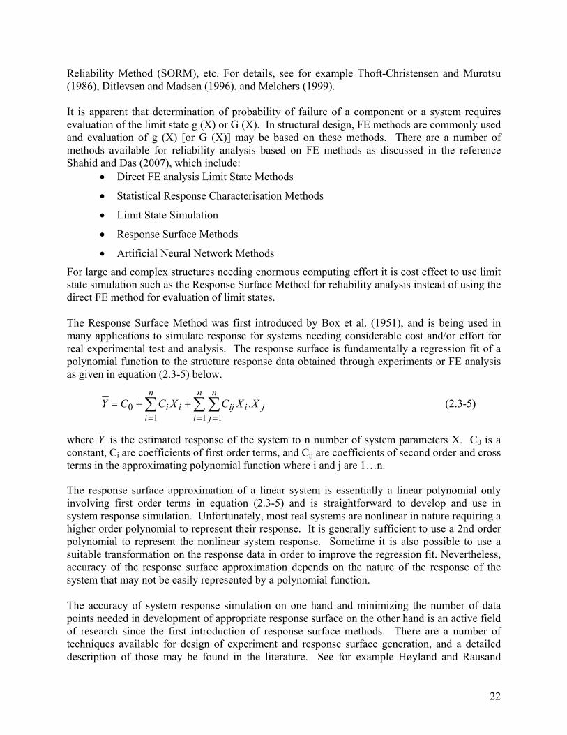
Reliability Method (SORM), etc. For details, see for example Thoft-Christensen and Murotsu (1986), Ditlevsen and Madsen (1996), and Melchers (1999). It is apparent that determination of probability of failure of a component or a system requires evaluation of the limit state g (X) or G (X). In structural design, FE methods are commonly used and evaluation of g (X) [or G (X)] may be based on these methods. There are a number of methods available for reliability analysis based on FE methods as discussed in the reference Shahid and Das (2007), which include:
• Direct FE analysis Limit State Methods
• Statistical Response Characterisation Methods
• Limit State Simulation
• Response Surface Methods
• Artificial Neural Network Methods
For large and complex structures needing enormous computing effort it is cost effect to use limit state simulation such as the Response Surface Method for reliability analysis instead of using the direct FE method for evaluation of limit states. The Response Surface Method was first introduced by Box et al. (1951), and is being used in many applications to simulate response for systems needing considerable cost and/or effort for real experimental test and analysis. The response surface is fundamentally a regression fit of a polynomial function to the structure response data obtained through experiments or FE analysis as given in equation (2.3-5) below.
∑ ∑∑= ==
++=n
i
n
jjiij
n
iii XXCXCCY
1 110 . (2.3-5)
where Y is the estimated response of the system to n number of system parameters X. C0 is a constant, Ci are coefficients of first order terms, and Cij are coefficients of second order and cross terms in the approximating polynomial function where i and j are 1…n. The response surface approximation of a linear system is essentially a linear polynomial only involving first order terms in equation (2.3-5) and is straightforward to develop and use in system response simulation. Unfortunately, most real systems are nonlinear in nature requiring a higher order polynomial to represent their response. It is generally sufficient to use a 2nd order polynomial to represent the nonlinear system response. Sometime it is also possible to use a suitable transformation on the response data in order to improve the regression fit. Nevertheless, accuracy of the response surface approximation depends on the nature of the response of the system that may not be easily represented by a polynomial function. The accuracy of system response simulation on one hand and minimizing the number of data points needed in development of appropriate response surface on the other hand is an active field of research since the first introduction of response surface methods. There are a number of techniques available for design of experiment and response surface generation, and a detailed description of those may be found in the literature. See for example Høyland and Rausand
22
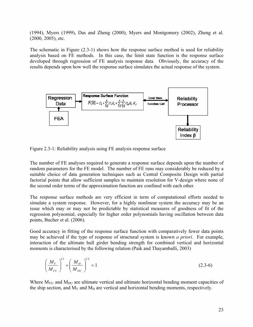
(1994), Myers (1999), Das and Zheng (2000), Myers and Montgomery (2002), Zheng et al. (2000, 2005), etc. The schematic in Figure (2.3-1) shows how the response surface method is used for reliability analysis based on FE methods. In this case, the limit state function is the response surface developed through regression of FE analysis response data. Obviously, the accuracy of the results depends upon how well the response surface simulates the actual response of the system.
Figure 2.3-1: Reliability analysis using FE analysis response surface
The number of FE analyses required to generate a response surface depends upon the number of random parameters for the FE model. The number of FE runs may considerably be reduced by a suitable choice of data generation techniques such as Central Composite Design with partial factorial points that allow sufficient samples to maintain resolution for V-design where none of the second order terms of the approximation function are confined with each other. The response surface methods are very efficient in term of computational efforts needed to simulate a system response. However, for a highly nonlinear system the accuracy may be an issue which may or may not be predictable by statistical measures of goodness of fit of the regression polynomial, especially for higher order polynomials having oscillation between data points, Bucher et al. (2006). Good accuracy in fitting of the response surface function with comparatively fewer data points may be achieved if the type of response of structural system is known a priori. For example, interaction of the ultimate hull girder bending strength for combined vertical and horizontal moments is characterised by the following relation (Paik and Thayamballi, 2003)
121
=⎟⎟⎠
⎞⎜⎜⎝
⎛+⎟⎟
⎠
⎞⎜⎜⎝
⎛C
HU
H
C
VU
V
MM
MM
(2.3-6)
Where MVU and MHU are ultimate vertical and ultimate horizontal bending moment capacities of the ship section, and MV and MH are vertical and horizontal bending moments, respectively.
23

Figure 2.3-2: Damaged ship structure, variables relevant for reliability based assessment of residual structural strength. In general, the ultimate strength of a damaged ship essentially depends upon the physical characteristics of structural damage such as the location of damage that include distance of centre of damage from the appropriate ship reference axis, and the size of the damaged part of the hull structure that includes damaged depth, damaged height and damaged width as shown in Figure (2.3-2). Other factors include the variation in properties of material used in construction of the hull and aging effects such as corrosion and accumulation of stress during active service of the ship (fatigue cycles). Accordingly, the residual ultimate strength of a damaged ship depicted by the ship’s ultimate moment capacity Mu may be given by the following: ),,,,,,,,,,,( ETDDDDDFMMMfM yagevldwhsthvu σ= (2.3-7) Where f (...) is the ultimate strength response function, which depends on the following parameters: Mv — vertical moment load Mh — horizontal moment load Mt — torsion load Fs — shear force load Dh — height of damaged structural part Dw — width of damaged structural part Dd — depth of damaged structural part Dl — longitudinal location of structural damage Dv — vertical location of structural damage Tage — aging related structural degradation
24

σy — yield strength of material E — Modulus of elasticity of the material The first four parameters pertaining to load and load combinations are essentially stochastic in nature because of random nature of the sea environment in which the ship operates along with the random operating profile of the ship experienced in service. The parameters relevant to size and location of structural damage are also random in nature and depend upon the type and nature of the incident that caused the damage. The aging related degradation in structural strength of ship might also be accounted for while making reliability-based assessment of residual strength of a ship having considerable time in service. The last two parameters, yield strength and modulus of elasticity of material used in construction of the ship are also random in nature and therefore should be part of a statistical/probabilistic assessment.
Figure 2.3-3: Number of random variables and computational effort
For an objective to provide quick assessment of residual ultimate strength of a damaged ship for
is considered an appropriate rmulation. However, the ultimate objective of the current research was to develop a reliability-
enings are ostly asymmetric giving way to a stress field in the damaged structure that will be much
decision support based on reliability and risk analysis to ensure her safe passage subsequent to a damage incident, the ultimate strength response function in (2.3-7) fobased design procedure for better assessment of the survivability of damaged ships and accordingly the response function may be modified to reduce the number of parameters that are directly relevant to design development. This also considerably reduces the computational effort required in development of the ultimate strength response function (see Figure 2.3-3). As far as the conventional design approach and differences in evaluation of damaged ship structure are concerned, the major deviation is in load combinations that arise because of large ship side openings subsequent to ship’s structure damage in collisions. Such opmdifferent from that of an intact ship. Furthermore, considerable residual stress is expected to exist subsequent to plastic rupture and damage of structure in a collision impact. As discussed earlier, the conventional design tools are developed for loading conditions that are predominantly
25

26
vertical, horizontal and torsion moment, spectively.
fixed size of structural damage as per the recommendation of classification society Lloyd’s
rties for reliability analysis are taken care of, along with other factors related to roduction such as residual stress, through modelling uncertainties parameters in the
for intact ships, viz. vertical bending moment and horizontal bending moment, respectively in order of precedence, for assessment of the ultimate strength of ships hull girders. For a damaged condition, the torsional moment is also likely to be a dominant load. In order to develop an ultimate strength model for a damaged ship hull girder, the following response model is adopted for reliability-based assessment of residual strength: ),,( thvu MMMfM = (2.3-8) Where Mv, Mh and Mt as mentioned earlier are re ARegister is given in Table 2.3-1 and is considered in this study. The random variations in material propepperformance function.
Table 2.3-1: LR Rules; collision damage extent
The extent of damage due to military threats defined as Military threats the minimum of the shock or blast damage that is likely
to result from a specified weapon threat. - 5 m longitudinally between
bulkheads Colli e
side shell sion damage to th Level A - from the waterline up to the main
deck - inboard for B/5 m

3. A SAMPLE VESSEL, ITS MODEL AND DAMAGE SCENARIOS 3.1 Descriptions of the Sample Vessel and Its Model A sample vessel, which is a notional US Navy destroyer, Hull 5415, was initially designed by the Naval Surface Warfare Center Carderock Division (NSWCCD). The principal dimensions of the vessel are shown in Table 3-1. Division of the compartments of the vessel is presented in Figure 3-1. The other details of Hull 5415 can be seen in Lee et al. (2006). Table 3-1: Main particulars of Hull 5415 and its model
Particulars Ship Model (1/100) Length overall (Loa) in meters 151.18 1.5118 Length between perpendiculars (Lpp) in meters 142.04 1.4204 Breadth moulded (B) in meters 20.03 0.2003 Depth to public spaces deck (D) in meters 12.74 0.1274 Design draft (T) in meters 6.31 0.06124 Maximum section area (Ax) in m2 96.7923 0.009679 Block coefficient (CB) 0.4909 0.4909 Prismatic coefficient (CP) 0.6409 0.6409 Midship section coefficient (CM) 0.7658 0.7658 KM (Height of metacentre above keel) in m 9.47 0.0947 Height of gravity centre above keel (KG) in meters 6.283 0.06817 Metacentric height (GM) in meters 3.187 0.02602 Longitudinal position CoG from A.P. (LCG) in meters 71.02 0.7168 Roll radius of gyration (kxx) in meters 0.0612 Pitch radius of gyration (kyy) in meters 0.3250 Yaw radius of gyration (kzz) in meters 0.3250
A ship model with a scale of 1/100 has been made from fibreglass based on the offsets of Hull 5415. Using such a small model scale is due to the dimensions of the towing tank facility. The main particulars of the model are presented in Table 3-1, while a view of the model is shown in Figure 3-2. As described in Chapter 2, in order to measure the wave-induced loads, the model is cut into two pieces at the cross-section, which is located 545 mm from the after perpendicular longitudinally. The two sections are linked together by a force gauge, which is bolted to two substantial bulkheads mounted in the fore and aft parts of the model and the two sections are made waterproof by the provision of a thin membrane across the cut. Although every effort has been made to construct a ship model with the same longitudinal weight distribution as the original ship, it proved to be very difficult to achieve this due to the general arrangement of the ship model, especially around the location of the force gauge, whose weight is a large percent of the total weight of the ship model. Therefore the ship model has
27

slightly different longitudinal weight distribution from the original ship. The longitudinal weight distributions of the original ship and ship model are presented in Figures 3-3 and 3-4.
Figure 3-1: Division of the compartments of the vessel
28

Figure 3-2: The ship model (Lee, et al. 2006)
Figure 3.3: Weight distribution of the intact sample vessel
Figure 3-4: Weight distribution of the intact model
29

For the hull girder loading measurements the model used for motion tests was converted by adding internal bulkheads and decks. In order to accomplish damaged model tests additional parts were built. T1 ~ T6 and D1 ~ D4 stand for transverse bulkheads and decks respectively. L1 and L2 stand for longitudinal girders (see Figure 3-5). No materials were placed inside the model to simulate permeability conditions. The size of the openings was less than the full length and height of the flooded area as will be described below. A general view of the damaged model for loading tests is shown in Figure 3-6.
Figure 3-5: Model compartmentation for damage containment
30

Figure 3-6: General view of the model for loading tests in damaged conditions It should be pointed out that the ship model used for this project was the same as that used for the NICOP project except for the way that the cut was sealed. Figures 3-7 and 3-8 show how the cling film was applied in both the NICOP and the current projects. In the NICOP project the film was applied as a flat surface, although it was fairly loose to minimise the effects of the cling film on the measurement of loads. However the cling film was still subject to loads to some extent. It should be noted that the effects of the cling film were very small (may be negligible) when the magnitude of loads was relatively large, such as vertical bending moment in head seas, etc. However the maximum torsion on the ship model was only about 0.3 N-m, and the effects of the cling film on torsion could be significant. In the current study, the cling film was tucked into the gap, so it would not be subject to any loads (ideally).
Gap Hull of the model
Tape The film
Figure 3-7: The cling film in the NICOP project
31

Figure 3-8: The cling film in the current project
mage scenarios have been used and are shown in Figures 3-9 to 3-11.
er
3.2 Damage Scenarios In this project, three daDetailed explanations of the reasons for using these damage scenarios can be seen in the report of Lee, et al. (2006). Presented in Figure 3-9 is damage scenario 1, which has a 5-metre long by 5.5-metre high opening in the starboard side shell in the middle of machine room 2 longitudinally as indicated by a rectangular window with dashed line. Because the lower edge of the opening is below the draught, water could enter the damaged machine room, which is indicated by the shaded areas. Water ingress is symmetrical transversely, so heel angle is zero at this scenario. This damage scenario simulates a possible collision at Level A, which is recommended in Lloyd’s Register Rules (Lloyd’s Register of Shipping, 2002). Model tests have not been carried out for this damage scenario due to the limited availability of the towing tank. However structural strength assessment has been applied to this scenario because damage is limited to only one compartment so that the size of finite element model is more manageable. Figure 3-10 shows damage scenario 2, which is similar to the damage sustained by the destroyUSS Cole (http://archives.cnn.com), which suffered from a 12-metre by 12-metre hole in the ship’s side shell caused by a suicide attack. Hence in this damage scenario, a 12-meter long by 9-meter high opening in the starboard side shell is introduced as indicated by a rectangular window with dashed line. The opening extends equally into machine rooms 2 and 3 longitudinally, and penetrates into the double bottom causing water ingress in four fuel tanks on the starboard side. Both experimental tests and numerical calculations have been applied to this damage scenario and to damage scenario 3, which is shown in Figure 3-11. Damage scenario 3 simulates a raking damage at Levels B & C as recommended in Lloyd’s Register Rules (Lloyd’s Register of Shipping, 2002). The damage is mainly in the bow and is symmetrical transversely. Table 3-2 presents the floating conditions of the sample ship in the intact and damaged conditions, while its intact stability is summarised in Table 3-3. Similarly the floating conditions of the ship model at intact and damaged conditions are shown in Table 3-4, and the intact stability is presented in Table 3-5. From those tables it can be seen that the sample vessel and its
Hull of the mo
Gap del
The film The tape
32

model have different draughts apart from their difference in longitudinal weight distribution and total weight at design draught. Damage scenario 2 has led to an increase of draught by 1.121 meters and a heel angle of 1.1 degree towards starboard. The reason for such a small heel angle is that the major flooding in machine rooms 2 and 3 is transversely symmetrical. The only unsymmetrical flooding is at the four small fuel tanks within the double bottom. This is the most severe damage among all the 3 damage scenarios. In damage scenario 3, the draught has increased the least by only 0.143 meters and the ship is not heeling. The transverse GM of the sample ship is 3.126 metres, so it has adequate stability.
Figure 3-9: Damage scenario 1
33

Figure 3-10: Damage scenario 2
34

Figure 3-11: Damage scenario 3
The draught, trim and heel angles were calculated to obtain the initial hydrostatic information using the UNEW Hydro programme and the programme HECSALV. For these calculations, the following compartment permeabilities were used. These compartment permeabilities were not used in the linear and nonlinear ship motions and loads analyses.
• Machinery spaces — 0.85 • Fuel oil tanks — 0.99 • Miscellaneous spaces — 0.85 • Sonar room — 0.85 • Forepeak tank — 0.99
35
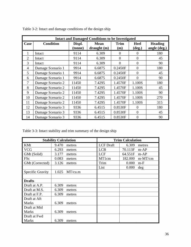
Table 3-2: Intact and damage conditions of the design ship
Intact and Damaged Conditions to be Investigated Case Condition Displ.
(tonne) Mean
draught (m) Trim (m)
Heel (deg.)
Heading angle (deg.)
1 Intact 9114 6.309 0 0 180 2 Intact 9114 6.309 0 0 45 3 Intact 9114 6.309 0 0 90 4 Damage Scenario 1 9914 6.6875 0.2450F 0 180 5 Damage Scenario 1 9914 6.6875 0.2450F 0 45 6 Damage Scenario 1 9914 6.6875 0.2450F 0 90 7 Damage Scenario 2 11450 7.4295 1.4570F 1.100S 180 8 Damage Scenario 2 11450 7.4295 1.4570F 1.100S 45 9 Damage Scenario 2 11450 7.4295 1.4570F 1.100S 90 10 Damage Scenario 2 11450 7.4295 1.4570F 1.100S 270 11 Damage Scenario 2 11450 7.4295 1.4570F 1.100S 315 12 Damage Scenario 3 9336 6.4515 0.8530F 0 180 13 Damage Scenario 3 9336 6.4515 0.8530F 0 45 14 Damage Scenario 3 9336 6.4515 0.8530F 0 90
Table 3-3: Intact stability and trim summary of the design ship
Stability Calculation Trim Calculation KMt 9.470 metres LCF Draft 6.309 metres VCG 6.293 metres LCB 70.113F m-AP GMt (Solid) 3.177 metres LCF 64.551F m-AP FSc 0.083 metres MT1cm 182.000 m-MT/cm GMt (Corrected) 3.126 metres Trim 0.000 m-F List 0.000 deg Specific Gravity 1.025 MT/cu.m Drafts Draft at A.P. 6.309 metres Draft at M.S. 6.309 metres Draft at F.P. 6.309 metres Draft at Aft Marks 6.309 metres Draft at Mid Marks 6.309 metres Draft at Fwd Marks 6.309 metres
36

KMt – Transverse metacentric height above baseline VCG – Vertical centre of gravity GMt (Solid)- The metacentric height FSc – Free surface correction GMt (Corrected) – The metacentric height with correction MT1cm – Moment to trim 1cm
Table 3-4: Intact and damage conditions of the ship model
Intact and Damaged Conditions to be Investigated Case Condition Displ.
(tonne) Mean
draught (m) Trim (m) Heel
(deg.) Heading
angle (deg.)
1 Intact 0.008503 0.06124 0 0 180 2 Intact 0.008503 0.06124 0 0 45 3 Intact 0.008503 0.06124 0 0 90 7 Damage Scenario 2 0.01145 0.072085 0.013350F 1.000S 180 8 Damage Scenario 2 0.01145 0.072085 0.013350F 1.000S 45 9 Damage Scenario 2 0.01145 0.072085 0.013350F 1.000S 90 10 Damage Scenario 2 0.01145 0.072085 0.013350F 1.000S 270 11 Damage Scenario 2 0.01145 0.072085 0.013350F 1.000S 315 12 Damage Scenario 3 0.008771 0.062635 0.007610F 0 180 13 Damage Scenario 3 0.008771 0.062635 0.007610F 0 45 14 Damage Scenario 3 0.008771 0.062635 0.007610F 0 90
37
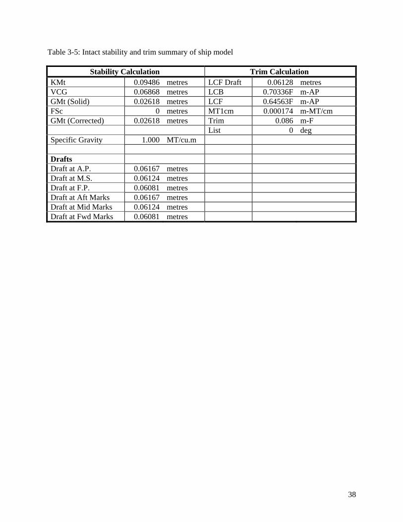
38
Table 3-5: Intact stability and trim summary of ship model
Stability Calculation Trim Calculation KMt 0.09486 metres LCF Draft 0.06128 metres VCG 0.06868 metres LCB 0.70336F m-AP GMt (Solid) 0.02618 metres LCF 0.64563F m-AP FSc 0 metres MT1cm 0.000174 m-MT/cm GMt (Corrected) 0.02618 metres Trim 0.086 m-F List 0 deg Specific Gravity 1.000 MT/cu.m Drafts Draft at A.P. 0.06167 metres Draft at M.S. 0.06124 metres Draft at F.P. 0.06081 metres Draft at Aft Marks 0.06167 metres Draft at Mid Marks 0.06124 metres Draft at Fwd Marks 0.06081 metres
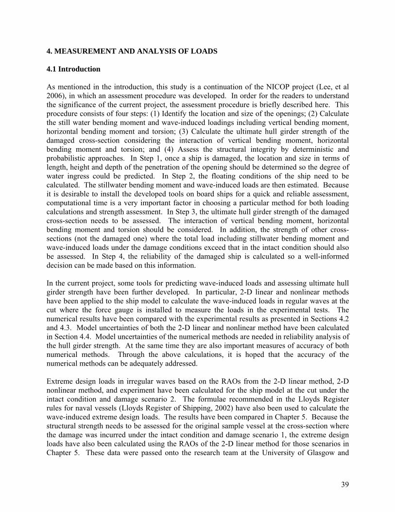
4. MEASUREMENT AND ANALYSIS OF LOADS 4.1 Introduction As mentioned in the introduction, this study is a continuation of the NICOP project (Lee, et al 2006), in which an assessment procedure was developed. In order for the readers to understand the significance of the current project, the assessment procedure is briefly described here. This procedure consists of four steps: (1) Identify the location and size of the openings; (2) Calculate the still water bending moment and wave-induced loadings including vertical bending moment, horizontal bending moment and torsion; (3) Calculate the ultimate hull girder strength of the damaged cross-section considering the interaction of vertical bending moment, horizontal bending moment and torsion; and (4) Assess the structural integrity by deterministic and probabilistic approaches. In Step 1, once a ship is damaged, the location and size in terms of length, height and depth of the penetration of the opening should be determined so the degree of water ingress could be predicted. In Step 2, the floating conditions of the ship need to be calculated. The stillwater bending moment and wave-induced loads are then estimated. Because it is desirable to install the developed tools on board ships for a quick and reliable assessment, computational time is a very important factor in choosing a particular method for both loading calculations and strength assessment. In Step 3, the ultimate hull girder strength of the damaged cross-section needs to be assessed. The interaction of vertical bending moment, horizontal bending moment and torsion should be considered. In addition, the strength of other cross-sections (not the damaged one) where the total load including stillwater bending moment and wave-induced loads under the damage conditions exceed that in the intact condition should also be assessed. In Step 4, the reliability of the damaged ship is calculated so a well-informed decision can be made based on this information. In the current project, some tools for predicting wave-induced loads and assessing ultimate hull girder strength have been further developed. In particular, 2-D linear and nonlinear methods have been applied to the ship model to calculate the wave-induced loads in regular waves at the cut where the force gauge is installed to measure the loads in the experimental tests. The numerical results have been compared with the experimental results as presented in Sections 4.2 and 4.3. Model uncertainties of both the 2-D linear and nonlinear method have been calculated in Section 4.4. Model uncertainties of the numerical methods are needed in reliability analysis of the hull girder strength. At the same time they are also important measures of accuracy of both numerical methods. Through the above calculations, it is hoped that the accuracy of the numerical methods can be adequately addressed. Extreme design loads in irregular waves based on the RAOs from the 2-D linear method, 2-D nonlinear method, and experiment have been calculated for the ship model at the cut under the intact condition and damage scenario 2. The formulae recommended in the Lloyds Register rules for naval vessels (Lloyds Register of Shipping, 2002) have also been used to calculate the wave-induced extreme design loads. The results have been compared in Chapter 5. Because the structural strength needs to be assessed for the original sample vessel at the cross-section where the damage was incurred under the intact condition and damage scenario 1, the extreme design loads have also been calculated using the RAOs of the 2-D linear method for those scenarios in Chapter 5. These data were passed onto the research team at the University of Glasgow and
39
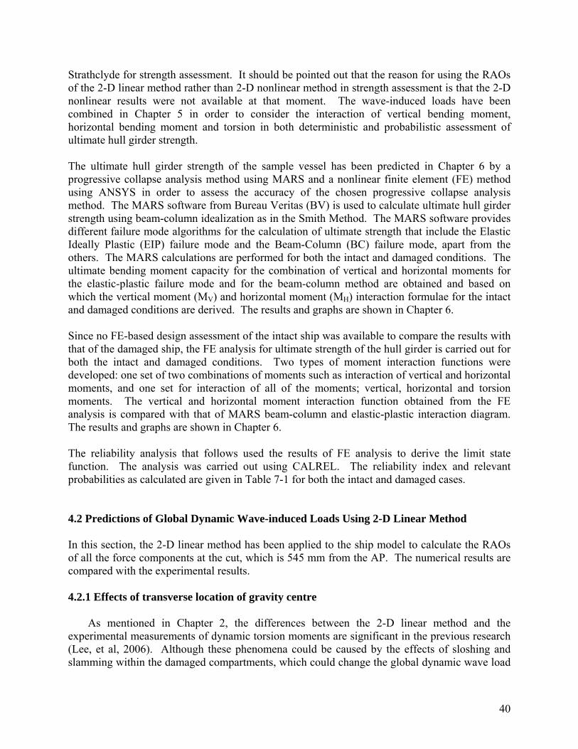
Strathclyde for strength assessment. It should be pointed out that the reason for using the RAOs of the 2-D linear method rather than 2-D nonlinear method in strength assessment is that the 2-D nonlinear results were not available at that moment. The wave-induced loads have been combined in Chapter 5 in order to consider the interaction of vertical bending moment, horizontal bending moment and torsion in both deterministic and probabilistic assessment of ultimate hull girder strength. The ultimate hull girder strength of the sample vessel has been predicted in Chapter 6 by a progressive collapse analysis method using MARS and a nonlinear finite element (FE) method using ANSYS in order to assess the accuracy of the chosen progressive collapse analysis method. The MARS software from Bureau Veritas (BV) is used to calculate ultimate hull girder strength using beam-column idealization as in the Smith Method. The MARS software provides different failure mode algorithms for the calculation of ultimate strength that include the Elastic Ideally Plastic (EIP) failure mode and the Beam-Column (BC) failure mode, apart from the others. The MARS calculations are performed for both the intact and damaged conditions. The ultimate bending moment capacity for the combination of vertical and horizontal moments for the elastic-plastic failure mode and for the beam-column method are obtained and based on which the vertical moment (MV) and horizontal moment (MH) interaction formulae for the intact and damaged conditions are derived. The results and graphs are shown in Chapter 6. Since no FE-based design assessment of the intact ship was available to compare the results with that of the damaged ship, the FE analysis for ultimate strength of the hull girder is carried out for both the intact and damaged conditions. Two types of moment interaction functions were developed: one set of two combinations of moments such as interaction of vertical and horizontal moments, and one set for interaction of all of the moments; vertical, horizontal and torsion moments. The vertical and horizontal moment interaction function obtained from the FE analysis is compared with that of MARS beam-column and elastic-plastic interaction diagram. The results and graphs are shown in Chapter 6. The reliability analysis that follows used the results of FE analysis to derive the limit state function. The analysis was carried out using CALREL. The reliability index and relevant probabilities as calculated are given in Table 7-1 for both the intact and damaged cases. 4.2 Predictions of Global Dynamic Wave-induced Loads Using 2-D Linear Method In this section, the 2-D linear method has been applied to the ship model to calculate the RAOs of all the force components at the cut, which is 545 mm from the AP. The numerical results are compared with the experimental results. 4.2.1 Effects of transverse location of gravity centre
As mentioned in Chapter 2, the differences between the 2-D linear method and the experimental measurements of dynamic torsion moments are significant in the previous research (Lee, et al, 2006). Although these phenomena could be caused by the effects of sloshing and slamming within the damaged compartments, which could change the global dynamic wave load
40

components, other factors, such as transverse distribution of weight, should also have effects on torsion. Hence the effects of the transverse distribution of weight on the torsion moments have been investigated. In the 2-D linear method these effects can be considered by using a transverse location of the weight centre of the whole vessel or of each section. In the current study a transverse location of the gravity centre (TCG) in each transverse section was used. Three different TCGs, 0, 2 and 4 centimetres apart from the central plane of the ship model for each transverse section are assumed to calculate the torsion moments of the ship model at the cut. The results are presented in Figures 4.2.1-1 to 4.2.1-5.
0.0000
0.0020
0.0040
0.0060
0.0080
0.0100
0.0120
0.0140
0.0 1.0 2.0 3.0 4.0 5.0 6.0 7.0
w*sqrt(L/g)
P4/(r
ho*g
*zet
a*L
2*B
)
2D linear theory w ith TCG = 0
2D linear theory w ith TCG = 2
2D linear theory w ith VCG = 4
Figure 4.2.1-1: Torsion moment RAO in intact condition in stern quartering waves
0.0000
0.0020
0.0040
0.0060
0.0080
0.0100
0.0120
0.0140
0.0 1.0 2.0 3.0 4.0 5.0 6.0 7.0
w*sqrt(L/g)
P4/(r
ho*g
*zet
a*L^
2*B
)
2D linear theory w ith TCG = 0
2D linear theory w ith TCG = 2
2D linear theory w ith VCG = 4
Figure 4.2.1-2: Torsion moment RAO in intact condition in bow quartering waves
41
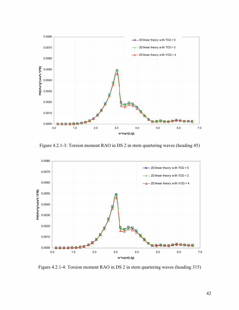
0.0000
0.0010
0.0020
0.0030
0.0040
0.0050
0.0060
0.0070
0.0080
0.0 1.0 2.0 3.0 4.0 5.0 6.0 7.0
w*sqrt(L/g)
P4/(r
ho*g
*zet
a*L^
2*B
)2D linear theory w ith TCG = 0
2D linear theory w ith TCG = 2
2D linear theory w ith VCG = 4
Figure 4.2.1-3: Torsion moment RAO in DS 2 in stern quartering waves (heading 45)
0.0000
0.0010
0.0020
0.0030
0.0040
0.0050
0.0060
0.0070
0.0080
0.0 1.0 2.0 3.0 4.0 5.0 6.0 7.0
w*sqrt(L/g)
P4/(r
ho*g
*zet
a*L^
2*B
)
2D linear theory w ith TCG = 0
2D linear theory w ith TCG = 2
2D linear theory w ith VCG = 4
Figure 4.2.1-4: Torsion moment RAO in DS 2 in stern quartering waves (heading 315)
42

0.0000
0.0020
0.0040
0.0060
0.0080
0.0100
0.0120
0.0140
0.0 1.0 2.0 3.0 4.0 5.0 6.0 7.0
w*sqrt(L/g)
P4/(r
ho*g
*zet
a*L^
2*B
)
2D linear theory w ith TCG = 0
2D linear theory w ith TCG = 2
2D linear theory w ith VCG = 4
Figure 4.2.1-5: Torsion moment RAO in DS 3 in stern quartering waves
These figures indicate that TCG has marginal effects on the torsion moments. The maximum difference tends to occur around the resonant regions, while the difference in other frequencies is noticeably smaller. The maximum difference at various conditions is summarised as follows:
• In the intact condition in stern quartering seas, the maximum difference is 10 percent. • In the intact condition in stern quartering seas, the maximum difference is 12.9
percent. • In damage scenario 2 in stern quartering seas (heading 45°), the maximum difference
is 14.5 percent. • In damage scenario 2 in stern quartering seas (heading 315°), the maximum
difference is 11 percent. • In damage scenario 3 in stern quartering seas, the maximum difference is 18.5
percent. Therefore the actual TCG of each transverse section has been estimated and used in the following calculations. 4.2.2 Results in intact condition The global dynamic wave induced loads calculated by the 2-D linear method and the experimental results in the intact condition in four different wave headings are presented in the following figures.
• Figures 4.2.2-1 to 4.2.2-5 for the intact condition in head waves. • Figures 4.2.2-6 to 4.2.2-10 for the intact condition in stern quartering waves. • Figures 4.2.2-11 to 4.2.2-15 for the intact condition in bow quartering waves.
43
• Figures 4.2.2-16 to 4.2.2-20 for the intact condition in beam waves. In the intact condition, the most important load is the vertical bending moment in head seas, which is shown in Figure 4.2.2-4. The results of the 2-D linear method agreed very well with the experimental results. The test results with small wave amplitude, which were plotted by square dots in the figure, appear to be closer to the solid line, which represents the numerical results than to those with large wave amplitude, which are indicated by triangles and diamond dots. This means that the 2-D linear method predicts the vertical bending moment more accurately at small wave amplitude than at large wave amplitude. This is understandable because the ship’s responses to small wave amplitudes are more likely to be in the linear range, so the results from a linear theory are expected to agree reasonably well with the experimental results. Nonlinear responses would normally occur in large wave amplitudes. More-detailed calculations in Section 4.4, in which model uncertainties of the 2-D linear method were predicted, provide quantitative support to this observation. As defined in Section 2.1.5, model uncertainty of a given method is a good measure of the accuracy of the method. When the model uncertainty factor (Xm) is equal to 1.0, it means that it is a 100 percent accurate result. The coefficient of variation (COV) of the model uncertainty factor measures how much dispersion there is in the calculations. The nearer the mean of Xm is to 1.0 and the smaller the COV of Xm is, the more accurate the numerical method is. The results in Table B-1 in Appendix B clearly support the above observations. The vertical bending moment in head seas had an Xm of 0.890 at the peak response, and a mean of Xm of 0.890 and a COV of Xm of 19.3 percent in small wave amplitudes. This accuracy is reasonably good. However the mean and COV of Xm become 0.773 and 24.5 percent for large wave amplitudes, and 0.750 and 27.4 percent for very large wave amplitudes. This demonstrates that the accuracy deteriorates with the increase of wave amplitude. Another interesting phenomenon shown in Figures 4.2.2-4, 4.2.2-9, and 4.2.2-14 about the vertical bending moment is that the measured RAOs are scattered in a large range for different wave amplitudes in the resonant region, where wave length is close to the ship model length. This may suggest that the responses have high level of nonlinearity at this condition. Similar features could also be observed in the results in damage scenarios 2 and 3. This high nonlinearity may well be an inherent feature of this particular hull form, which is a typical destroyer with a small block coefficient. In addition, the cut, where the loads were measured, was close to the stern region with sharp change of water-plane width. This is normally another major source of nonlinear responses. To further verify this, a second batch of experimental tests has been carried out, and the results will be presented in Section 4.2.5. The numerical predictions of vertical bending moments in quartering seas are also in good agreement with experimental results as shown in Figures 4.2.2-9 and 4.2.2-14. The mean and COV of Xm at small amplitudes are 1.01 and 31.9 percent, respectively, in stern quartering seas, while they are 0.86 and 24.6 percent in bow quartering seas (see Table B1). As shown in Figure 4.2.2-19, the differences of the vertical bending moment between the numerical and experimental results in beam waves are significant. Nevertheless the magnitude of loads in beam waves is usually very small, so the large difference would not cause much concern in the strength assessment of hull girders.
44

Horizontal bending moments and torsion in quartering seas, which are shown in Figures 4.2.2-8, 4.2.2-10, 4.2.2-13, and 4.2.2-15, are also important force components. The curves of horizontal bending moment predicted by the 2-D linear method have double peaks, while the peak of the test data is falling in between the peaks of the numerical results (see Figures 4.2.2-10 and 4.2.2-15). It is this shift of peaks that causes large differences between the numerical and experimental results. The mean and COV of Xm at small amplitude are 1.12 and 70.5 percent respectively in stern quartering seas, while they are 0.78 and 67.3 percent in bow quartering seas (see Table B1). Although the mean of Xm at small amplitude in stern quartering seas looks reasonably good, its COV is quite large. Further scrutiny of the individual figures of Xm has revealed that five out of nine have more than 50 percent error, and only 2 of them have less than 20 percent error. Especially, the Xm around the resonant region have a value of 1.92 and 2.65, which are far away from 1.0. The accuracy of the prediction around the resonant region is more important than those in other frequencies because the current load combination method uses the load in this area for strength assessment. Similar features could be seen for Xm in bow quartering seas. Therefore the accuracy in predicting horizontal bending moments is not as good as that for vertical bending moments. The disappointing accuracy in horizontal bending moment prediction might be caused partly by the mooring lines in the experimental tests. As described in Section 2.1.4, the ship model was moored by four mooring lines, which were attached to the ends of the model to keep the model from drifting too far away from its original position and orientation (see Figure 2.1-3). It is a very delicate process to adjust the tensions in the mooring lines. On one hand, the tensions should be as small as possible to reduce their effects on the responses to waves. On the other hand, the model could not maintain its original position and direction if the tensions in the mooring lines were too small. So during the test, the mooring lines were initially fixed fairly loosely. A trial run was then carried out. If the model drifted too far away, the tension would be increased. However if the tension in the mooring lines were clearly interfering with the ship motions under waves, the tension would be reduced. Hence a delicate compromise had to be achieved. Even so, the tensions in the mooring lines were still noticeable in the resonant frequencies, in which responses were quite large in the recorded test runs. The tensions in the mooring lines could contribute to the horizontal bending moment at the cut. Unfortunately the tensions were not recorded in the tests, so it was not possible to evaluate the extent of the effects of the tensions on the horizontal bending moment. Figures 4.2.2-8 and 4.2.2-13 present torsion moments in quartering seas. It can be seen that the numerical results were very different from the experimental results. This large difference comes from two major issues, one of which is the shift of peaks in between the numerical and experimental results while the other is the difference in magnitude even if the peaks were achieved at the same frequency. The mean and COV of Xm at small amplitude are 0.96 and 135.9 percent, respectively, in stern quartering seas, while they are 0.56 and 60.3 percent in bow quartering seas (see Table B1). Although the mean of Xm at small amplitudes in stern quartering seas looks very good, its COV is too large. Further investigation into the individual figures of Xm has revealed that the values vary from 0.18 to 4.25, and the nearest figure to 1.0 is 0.85 at the highest frequency. Similarly in bow quarter seas the mean and COV are equally bad. Therefore the predictions of torsion moment were considered as being very poor.
45

One of the possible reasons for such a poor performance in torsion moment prediction might be the small scale of the ship model, which is 1/100. The maximum measured torsion is only about 0.3 N-m, so its measurement is very sensitive to any imperfections, such as the quality of installation of the cling film, which was used to seal the cut section of the model; calibration of the instruments; electrical noise in the records; etc. The other possible reason is the inherent difficulty in determining the radius of gyration for roll motion (kxx) and the damping coefficient for roll motion, which is a very important motion component influencing the accuracy of the prediction of torsion moments. Head waves
0.00
0.01
0.02
0.03
0.04
0.05
0.06
0.07
0.0 1.0 2.0 3.0 4.0 5.0 6.0 7
w*sqrt(L/g)
P2/(r
ho*g
*zet
a*L*
B)
.0
Wave height = small
Wave height = large
w ave height=very large
2D linear theroy w ith estimated TCG
Figure 4.2.2-1: Horizontal shear force RAO in intact condition in head waves
46

0.000
0.010
0.020
0.030
0.040
0.050
0.060
0.070
0.080
0.0 1.0 2.0 3.0 4.0 5.0 6.0 7.0
w*sqrt(L/g)
P3/(r
ho*g
*zet
a*L*
B)
Wave height = small
Wave height = large
Wave height = very large
2D linear theory w ith estimated TCG
Figure 4.2.2-2: Vertical shear force RAO in intact condition in head waves
0.0000
0.0001
0.0002
0.0003
0.0004
0.0005
0.0006
0.0007
0.0008
0.0009
0.0010
0.0 1.0 2.0 3.0 4.0 5.0 6.0 7.0
w*sqrt(L/g)
P4/(r
ho*g
*zet
a*L^
2*B
)
Wave height = small
Wave height = large
Wave height = very large
2D linear theory w ith estimated TCG
Figure 4.2.2-3: Torsion moment RAO in intact condition in head waves
47

0.000
0.005
0.010
0.015
0.020
0.0 1.0 2.0 3.0 4.0 5.0 6.0 7w*sqrt(L/g)
P5/(r
ho*g
*zet
a*L^
2*B
)
.0
Wave height = small
Wave height = large
Wave height = very large
2D linear theory w ith estimated TCG
Figure 4.2.2-4: Vertical bending moment RAO in intact condition in head waves
0.000
0.002
0.004
0.006
0.008
0.010
0.012
0.0 1.0 2.0 3.0 4.0 5.0 6.0 7.0
w*sqrt(L/g)
P6/(r
ho*g
*zet
a*L
2*B
)
Wave height = small
Wave height = large
Wave height = very large
2D linear theory w ith estimated TCG
Figure 4.2.2-5: Horizontal bending moment RAO in intact condition in head waves
48

Stern quartering waves
0.00
0.01
0.02
0.03
0.04
0.05
0.06
0.07
0.08
0.09
0.10
0.0 1.0 2.0 3.0 4.0 5.0 6.0
w*sqrt(L/g)
P2/(r
ho*g
*zet
a*L*
B)
7.0
Wave height = small
Wave height = large
w ave height=very large
2D linear theroy w ith estimated TCG
Figure 4.2.2-6: Horizontal shear force in intact condition in stern quartering waves
0.000
0.010
0.020
0.030
0.040
0.050
0.060
0.070
0.080
0.090
0.100
0.0 1.0 2.0 3.0 4.0 5.0 6.0 7w*sqrt(L/g)
P3/(r
ho*g
*zet
a*L*
B)
.0
Wave height = small
Wave height = large
Wave height = very large
2D linear theory w ith estimated TCG
Figure 4.2.2-7: Vertical shear force RAO of intact condition in stern quartering waves
49
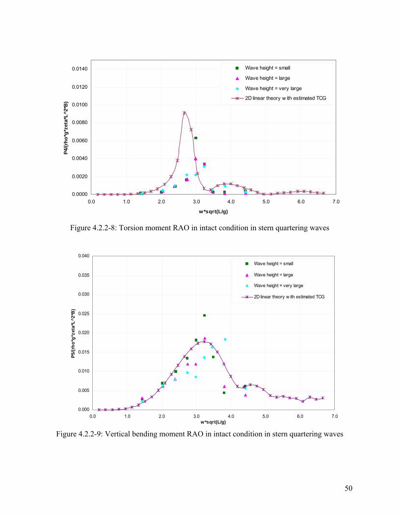
0.0000
0.0020
0.0040
0.0060
0.0080
0.0100
0.0120
0.0140
0.0 1.0 2.0 3.0 4.0 5.0 6.0 7.
w*sqrt(L/g)
P4/(r
ho*g
*zet
a*L^
2*B
)
0
Wave height = small
Wave height = large
Wave height = very large
2D linear theory w ith estimated TCG
Figure 4.2.2-8: Torsion moment RAO in intact condition in stern quartering waves
0.000
0.005
0.010
0.015
0.020
0.025
0.030
0.035
0.040
0.0 1.0 2.0 3.0 4.0 5.0 6.0 7.0w*sqrt(L/g)
P5/(r
ho*g
*zet
a*L^
2*B
)
Wave height = small
Wave height = large
Wave height = very large
2D linear theory w ith estimated TCG
Figure 4.2.2-9: Vertical bending moment RAO in intact condition in stern quartering waves
50

0.000
0.002
0.004
0.006
0.008
0.010
0.012
0.014
0.016
0.018
0.020
0.0 1.0 2.0 3.0 4.0 5.0 6.0 7
w*sqrt(L/g)
P6/(r
ho*g
*zet
a*L
2*B
)
.0
Wave height = small
Wave height = large
Wave height = very large
2D linear theory w ith estimated TCG
Figure 4.2.2-10: Horizontal bending moment RAO in intact condition in stern quartering waves
Bow quartering waves
0.00
0.01
0.02
0.03
0.04
0.05
0.06
0.07
0.0 1.0 2.0 3.0 4.0 5.0 6.0 7.0
w*sqrt(L/g)
P2/(r
ho*g
*zet
a*L*
B)
Wave height = small
Wave height = large
w ave height=very large
2D linear theroy w ith estimatedTCG
Figure 4.2.2-11: Horizontal shear force RAO in intact condition in bow quartering waves
51

0.000
0.010
0.020
0.030
0.040
0.050
0.060
0.0 1.0 2.0 3.0 4.0 5.0 6.0 7.0w*sqrt(L/g)
P3/(r
ho*g
*zet
a*L*
B)
Wave height = small
Wave height = large
Wave height = very large
2D linear theory w ithestimated TCG
Figure 4.2.2-12: Vertical shear force RAO in intact condition in bow quartering waves
0.0000
0.0020
0.0040
0.0060
0.0080
0.0100
0.0120
0.0 1.0 2.0 3.0 4.0 5.0 6.0 7.0
w*sqrt(L/g)
P4/(r
ho*g
*zet
a*L^
2*B
)
Wave height = small
Wave height = large
Wave height = very large
2D linear theory w ithestimated TCG
Figure 4.2.2-13: Torsion moment RAO in intact condition in bow quartering waves
52

0.000
0.005
0.010
0.015
0.020
0.0 1.0 2.0 3.0 4.0 5.0 6.0 7w*sqrt(L/g)
P5/(r
ho*g
*zet
a*L^
2*B
)
.0
Wave height = small
Wave height = large
Wave height = very large
2D linear theory w ithestimated TCG
Figure 4.2.2-14: Vertical bending moment RAO in intact condition in bow quartering waves
0.000
0.002
0.004
0.006
0.008
0.010
0.012
0.0 1.0 2.0 3.0 4.0 5.0 6.0 7.0
w*sqrt(L/g)
P6/(r
ho*g
*zet
a*L^
2*B
)
Wave height = small
Wave height = large
Wave height = very large
2D linear theory w ithestimated TCG
Figure 4.2.2-15: Horizontal bending moment RAO in intact condition in bow quartering waves
53

Beam waves
0.00
0.01
0.02
0.03
0.04
0.05
0.06
0.07
0.08
0.09
0.10
0.0 1.0 2.0 3.0 4.0 5.0 6.0 7
w*sqrt(L/g)
P2/(r
ho*g
*zet
a*L*
B)
.0
Wave height = small
Wave height = large
w ave height=very large
2D linear theroy w ithestimated TCG
Figure 4.2.2-16: Horizontal shear force RAO in intact condition in beam waves
0.000
0.010
0.020
0.030
0.040
0.050
0.060
0.0 1.0 2.0 3.0 4.0 5.0 6.0 7.0w*sqrt(L/g)
P3/(r
ho*g
*zet
a*L*
B)
Wave height = small
Wave height = large
Wave height = very large
2D linear theory w ithestimated TCG
Figure 4.2.2-17: Vertical shear force RAO in intact condition in beam waves
54

0.0000
0.0020
0.0040
0.0060
0.0080
0.0100
0.0120
0.0140
0.0 1.0 2.0 3.0 4.0 5.0 6.0 7.0w*sqrt(L/g)
P4/(r
ho*g
*zet
a*L^
2*B
)
Wave height = small
Wave height = large
Wave height = very large
2D linear theory w ith estimatedTCG
Figure 4.2.2-18: Torsion moment RAO in intact condition in beam waves
0.000
0.005
0.010
0.015
0.020
0.0 1.0 2.0 3.0 4.0 5.0 6.0 7.0w*sqrt(L/g)
P5/(r
ho*g
*zet
a*L^
2*B
)
Wave height = small
Wave height = large
Wave height = very large
2D linear theory w ith estimatedTCG
Figure 4.2.2-19: Vertical bending moment RAO in intact condition in beam waves
55

0.000
0.002
0.004
0.006
0.008
0.010
0.012
0.0 1.0 2.0 3.0 4.0 5.0 6.0 7.0
w*sqrt(L/g)
P6/(r
ho*g
*zet
a*L^
2*B
)
Wave height = small
Wave height = large
Wave height = very large
2D linear theory w ithestimated TCG
Figure 4.2.2-20: Horizontal bending moment RAO in intact condition in beam waves
4.2.3 Results in damage scenario 2 As mentioned in Chapter 3, in damage scenario 2 the ship model has an increase of draught by 1.09 centimetres (equivalent to 1.09 metres for the ship) and a heel angle of 1.1 degree towards starboard. The results in five different wave headings are presented in the following figures.
• Figures 4.2.3-1 to 4.2.3-5 for head waves. • Figures 4.2.3-6 to 4.2.3-10 for stern quartering waves (β = 45). • Figures 4.2.3-11 to 4.2.3-15 for stern quartering waves (β = 315). • Figures 4.2.3-16 to 4.2.3-20 for beam waves (β = 90). • Figures 4.2.3-21 to 4.2.3-25 for beam waves (β = 270).
The results for the vertical bending moment in head seas are shown in Figure 4.2.3-4. Generally speaking, the numerical results are in good agreement with the experimental results. In the resonant region, the numerical results agree better with the experimental results in small amplitude waves than in large amplitude waves. Quantitative comparisons have been presented in Table B.2 in Appendix B. It can be seen that the mean and COV of Xm are 0.789 and 27.0 percent for small wave amplitudes, and 0.740 and 21.4 percent for large wave amplitudes, and 0.783 and 18.3 percent for very large wave amplitudes. Because the damage is unsymmetrical transversely, it is expected that the wave-induced loads might be different when the wave is approaching the ship model from different sides due to the dynamic behaviour of the flooded water in the damaged compartment. Therefore two wave headings have been chosen for stern quartering seas; one is approaching from the starboard side (the damaged side), the other is from the port side. The 2-D linear method has produced
56

satisfactory results in both stern quartering seas in vertical bending moment predictions, as shown in Figures 4.2.3-9 and 4.2.3-14. The mean and COV of Xm are 1.063 and 28.2 percent in stern quartering seas from the starboard side for small wave amplitudes, and are 0.989 and 29.9 percent in stern quartering seas from the port side for small wave amplitudes. Therefore accuracy in both stern-quartering seas is of a similar level. To clearly demonstrate the difference caused by different approach angles, the vertical bending moments at 45° and 315° wave headings have been plotted together in Figure 4.2.3-26. Because the 2-D linear method can’t consider the effects of dynamic behaviour of flooded water and the heel angle is very small, the numerical results were nearly identical in both stern-quartering seas. However, the test results have shown that the vertical bending moment at a 45° wave heading at most of frequencies was slightly larger than that at a 315° wave heading. The vertical bending moment in beam seas, which are shown in Figures 4.2.3-19 and 4.2.3-24, was not significant, so there is no need for further discussion. Figures 4.2.3-10 and 4.2.3-15 show the results of horizontal bending moments in both stern quartering seas. The agreement between the 2-D linear method and experiment were reasonably good, although it was not as good as that in vertical bending moment predictions. The mean and COV of Xm are 1.164 and 67.2 percent in stern quartering seas from starboard for small wave amplitudes, and are 1.016 and 42.3 percent in stern quartering seas from port for small wave amplitudes. Therefore the accuracy in stern quartering seas from the port side is slightly better than that from the starboard side. It is also true for large and very large wave amplitudes (see Table B.2). The horizontal bending moment at 45° and 315° wave headings has been plotted together in Figure 4.2.3-27 to see how much difference was caused by these different approaching angles. There was no clear trend in this figure. Horizontal bending moments in both beam seas (from the starboard and port sides) is shown Figures 4.2.3-20 and 4.2.3-25. The large difference between the numerical and experimental results mainly occurs at either very low frequencies or very high frequencies. The mean and COV of Xm are 1.941 and 60.9 percent in beam seas from starboard for small wave amplitudes, and are 1.587 and 76.3 percent in beam seas from port for small wave amplitudes. The mean values in beam seas were not as good as in quartering seas. Similarly, the horizontal bending moments in beam seas at 90° and 270° wave headings has been plotted together in Figure 4.2.3-28. It is seen that the horizontal bending moment is slightly larger when the wave is approaching from the starboard side than that from the port side. Figures 4.2.3-8 and 4.2.3-13 show the results of torsion moments in both stern quartering seas. The agreement between the 2-D linear method and experiment were reasonably good. The method’s accuracy was not as good as that in vertical bending moment predictions, but surprisingly, was at a similar level to that in horizontal bending moment predictions. Unlike in intact conditions, the predicted frequency, where the maximum responses occur, matched reasonably well with measured frequency in the tests. The mean and COV of Xm are 0.633 and 64.1 percent in stern quartering seas from starboard for small wave amplitude, and are 0.828 and 52.6 percent in stern quartering seas from port for small wave amplitude. Therefore the accuracy in stern quartering seas from the port side is slightly better than that from the starboard side. It is also true for large and very large wave amplitudes (see Table B.2). The torsion moments at 45°
57
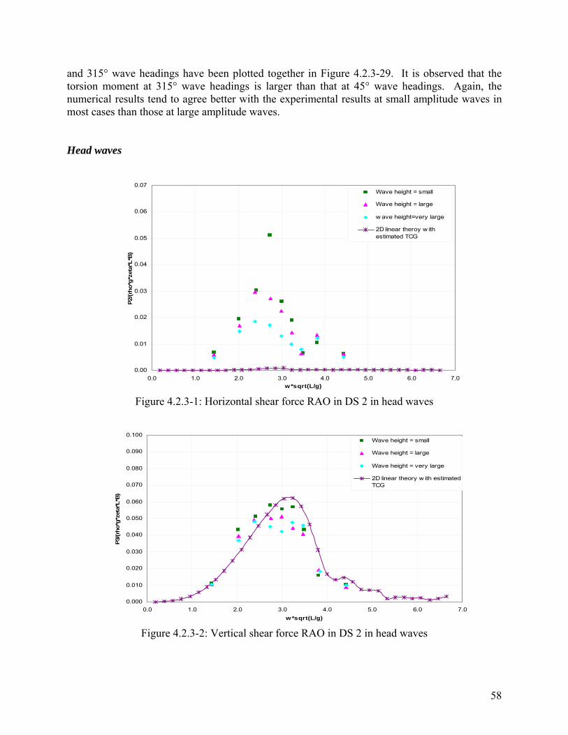
and 315° wave headings have been plotted together in Figure 4.2.3-29. It is observed that the torsion moment at 315° wave headings is larger than that at 45° wave headings. Again, the numerical results tend to agree better with the experimental results at small amplitude waves in most cases than those at large amplitude waves. Head waves
0.00
0.01
0.02
0.03
0.04
0.05
0.06
0.07
0.0 1.0 2.0 3.0 4.0 5.0 6.0 7.0w*sqrt(L/g)
P2/(r
ho*g
*zet
a*L*
B)
Wave height = small
Wave height = large
w ave height=very large
2D linear theroy w ithestimated TCG
Figure 4.2.3-1: Horizontal shear force RAO in DS 2 in head waves
0.000
0.010
0.020
0.030
0.040
0.050
0.060
0.070
0.080
0.090
0.100
0.0 1.0 2.0 3.0 4.0 5.0 6.0 7.0w*sqrt(L/g)
P3/(r
ho*g
*zet
a*L*
B)
Wave height = small
Wave height = large
Wave height = very large
2D linear theory w ith estimatedTCG
Figure 4.2.3-2: Vertical shear force RAO in DS 2 in head waves
58

0.0000
0.0005
0.0010
0.0015
0.0020
0.0025
0.0030
0.0 1.0 2.0 3.0 4.0 5.0 6.0 7.0w*sqrt(L/g)
P4/(r
ho*g
*zet
a*L
2*B
)Wave height = small
Wave height = large
Wave height = very large
2D linear theory w ithestimated TCG
Figure 4.2.3-3: Torsion moment RAO in DS 2 in head waves
0.000
0.005
0.010
0.015
0.020
0.025
0.0 1.0 2.0 3.0 4.0 5.0 6.0w*sqrt(L/g)
P5/(r
ho*g
*zet
a*L
2*B
)
7.0
Wave height = small
Wave height = large
Wave height = very large
2D linear theory w ith estimatedTCG
Figure 4.2.3-4: Vertical bending moment RAO in DS 2 in head waves
59

0.000
0.002
0.004
0.006
0.008
0.010
0.012
0.0 1.0 2.0 3.0 4.0 5.0 6.0 7
w*sqrt(L/g)
P6/(r
ho*g
*zet
a*L
2*B
)
.0
Wave height = small
Wave height = large
Wave height = very large
2D linear theory w ith estimatedTCG
Figure 4.2.3-5: Horizontal bending moment RAO in DS 2 in head waves
Stern quartering waves from starboard side (heading 45)
0.00
0.01
0.02
0.03
0.04
0.05
0.06
0.07
0.0 1.0 2.0 3.0 4.0 5.0 6.0 7.
w*sqrt(L/g)
P2/(r
ho*g
*zet
a*L*
B)
0
Wave height = small
Wave height = large
w ave height=very large
2D linear theroy w ithestimated TCG
Figure 4.2.3-6: Horizontal shear force RAO in DS 2 in stern quartering waves
60
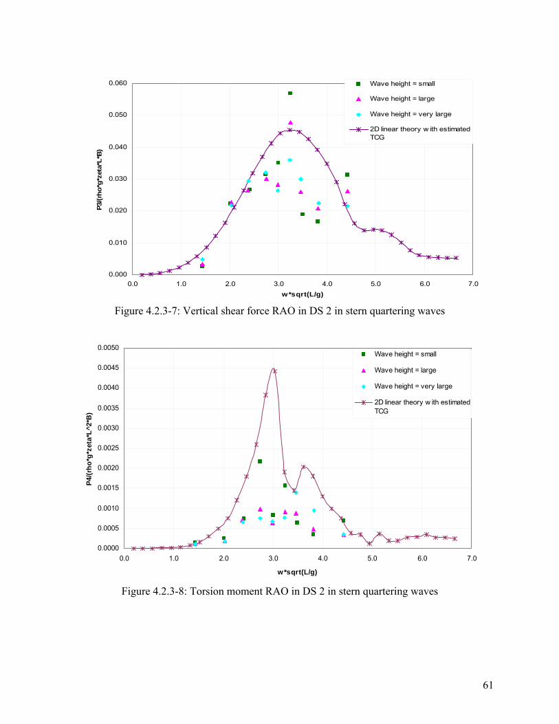
0.000
0.010
0.020
0.030
0.040
0.050
0.060
0.0 1.0 2.0 3.0 4.0 5.0 6.0 7.0w*sqrt(L/g)
P3/(r
ho*g
*zet
a*L*
B)
Wave height = small
Wave height = large
Wave height = very large
2D linear theory w ith estimatedTCG
Figure 4.2.3-7: Vertical shear force RAO in DS 2 in stern quartering waves
0.0000
0.0005
0.0010
0.0015
0.0020
0.0025
0.0030
0.0035
0.0040
0.0045
0.0050
0.0 1.0 2.0 3.0 4.0 5.0 6.0 7.0
w*sqrt(L/g)
P4/(r
ho*g
*zet
a*L^
2*B
)
Wave height = small
Wave height = large
Wave height = very large
2D linear theory w ith estimatedTCG
Figure 4.2.3-8: Torsion moment RAO in DS 2 in stern quartering waves
61

0.000
0.005
0.010
0.015
0.020
0.025
0.030
0.0 1.0 2.0 3.0 4.0 5.0 6.0 7.0w*sqrt(L/g)
P5/(r
ho*g
*zet
a*L^
2*B
)Wave height = small
Wave height = large
Wave height = very large
2D linear theory w ith estimatedTCG
Figure 4.2.3-9: Vertical bending moment RAO in DS 2 in stern quartering waves
0.000
0.002
0.004
0.006
0.008
0.010
0.012
0.0 1.0 2.0 3.0 4.0 5.0 6.0 7.0
w*sqrt(L/g)
P6/(r
ho*g
*zet
a*L
2*B
)
Wave height = small
Wave height = large
Wave height = very large
2D linear theory w ith estimatedTCG
Figure 4.2.3-10: Horizontal bending moment RAO in DS 2 in stern quartering waves
62

Stern quartering waves from the port side (heading 315)
0.00
0.01
0.02
0.03
0.04
0.05
0.06
0.07
0.0 1.0 2.0 3.0 4.0 5.0 6.0 7.0
w*sqrt(L/g)
P2/(r
ho*g
*zet
a*L*
B)
Wave height = small
Wave height = large
w ave height=very large
2D linear theroy w ithestimated TCG
Figure 4.2.3-11: Horizontal shear force RAO in DS 2 in stern quartering waves (heading 315)
0.000
0.010
0.020
0.030
0.040
0.050
0.060
0.0 1.0 2.0 3.0 4.0 5.0 6.0 7.0w*sqrt(L/g)
P3/(r
ho*g
*zet
a*L*
B)
Wave height = small
Wave height = large
Wave height = very large
2D linear theory w ithestimated TCG
Figure 4.2.3-12: Vertical shear force RAO in DS 2 in stern quartering waves (heading 315)
63

0.0000
0.0005
0.0010
0.0015
0.0020
0.0025
0.0030
0.0035
0.0040
0.0045
0.0050
0.0 1.0 2.0 3.0 4.0 5.0 6.0 7.0
w*sqrt(L/g)
P4/(r
ho*g
*zet
a*L^
2*B
)Wave height = small
Wave height = large
Wave height = very large
2D linear theory w ith estimatedTCG
Figure 4.2.3-13: Torsion moment RAO in DS 2 in stern quartering waves (heading 315)
0.000
0.005
0.010
0.015
0.020
0.025
0.030
0.0 1.0 2.0 3.0 4.0 5.0 6.0 7.0w*sqrt(L/g)
P5/(r
ho*g
*zet
a*L^
2*B
)
Wave height = small
Wave height = large
Wave height = very large
2D linear theory w ith estimatedTCG
Figure 4.2.3-14: Vertical bending moment RAO in DS 2
in stern quartering waves (heading 315)
64

0.000
0.002
0.004
0.006
0.008
0.010
0.012
0.014
0.0 1.0 2.0 3.0 4.0 5.0 6.0 7.0
w*sqrt(L/g)
P6/(r
ho*g
*zet
a*L^
2*B
)Wave height = small
Wave height = large
Wave height = very large
2D linear theory w ithestimated TCG
Figure 4.2.3-15: Horizontal bending moment RAO in DS 2
in stern quartering waves (heading 315)
Beam waves from the starboard side (heading 90)
0.00
0.02
0.04
0.06
0.08
0.10
0.12
0.14
0.16
0.18
0.20
0.0 1.0 2.0 3.0 4.0 5.0 6.0 7.0
w*sqrt(L/g)
P2/(r
ho*g
*zet
a*L*
B)
Wave height = small
Wave height = large
w ave height=very large
2D linear theroy w ith estimatedVCG
Figure 4.2.3-16: Horizontal shear force RAO in DS 2 in beam waves (heading 90)
65
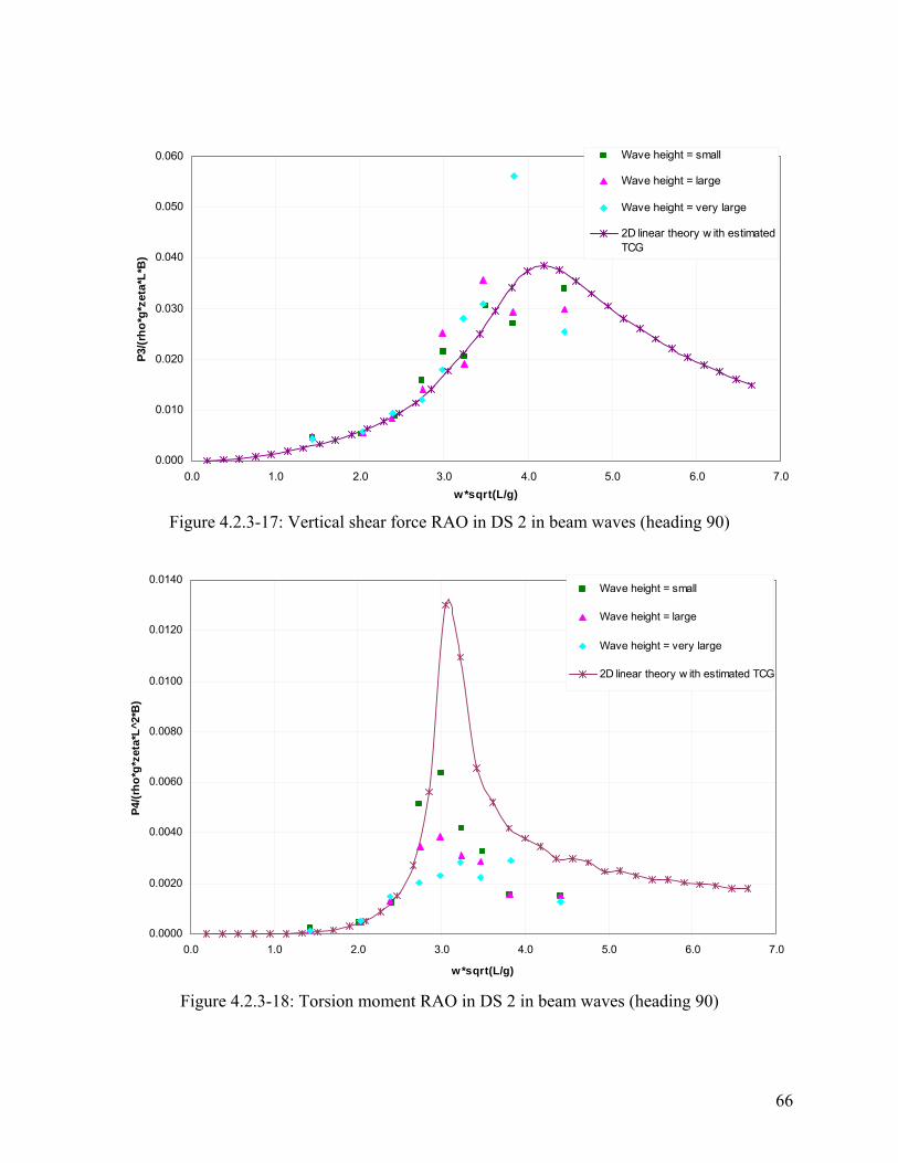
0.000
0.010
0.020
0.030
0.040
0.050
0.060
0.0 1.0 2.0 3.0 4.0 5.0 6.0 7.0w*sqrt(L/g)
P3/(r
ho*g
*zet
a*L*
B)
Wave height = small
Wave height = large
Wave height = very large
2D linear theory w ith estimatedTCG
Figure 4.2.3-17: Vertical shear force RAO in DS 2 in beam waves (heading 90)
0.0000
0.0020
0.0040
0.0060
0.0080
0.0100
0.0120
0.0140
0.0 1.0 2.0 3.0 4.0 5.0 6.0 7.0
w*sqrt(L/g)
P4/(r
ho*g
*zet
a*L^
2*B
)
Wave height = small
Wave height = large
Wave height = very large
2D linear theory w ith estimated TCG
Figure 4.2.3-18: Torsion moment RAO in DS 2 in beam waves (heading 90)
66

0.000
0.005
0.010
0.015
0.020
0.0 1.0 2.0 3.0 4.0 5.0 6.0 7.0w*sqrt(L/g)
P5/(r
ho*g
*zet
a*L^
2*B
)Wave height = small
Wave height = large
Wave height = very large
2D linear theory w ithestimated TCG
Figure 4.2.3-19: Vertical bending moment RAO in DS 2 in beam waves (heading 90)
0.000
0.002
0.004
0.006
0.008
0.010
0.012
0.0 1.0 2.0 3.0 4.0 5.0 6.0 7
w*sqrt(L/g)
P6/(r
ho*g
*zet
a*L^
2*B
)
.0
Wave height = small
Wave height = large
Wave height = very large
2D linear theory w ithestimated TCG
Figure 4.2.3-20: Horizontal bending moment RAO in DS 2 in beam waves (heading 90)
67

Beam waves from the port side (heading 270)
0.00
0.01
0.02
0.03
0.04
0.05
0.06
0.07
0.08
0.09
0.10
0.0 1.0 2.0 3.0 4.0 5.0 6.0 7
w*sqrt(L/g)
P2/(r
ho*g
*zet
a*L*
B)
.0
Wave height = small
Wave height = large
w ave height=very large
2D linear theroy w ithestimated TCG
Figure 4.2.3-21: Horizontal shear force RAO in DS 2 in beam waves (heading 270)
0.000
0.010
0.020
0.030
0.040
0.050
0.060
0.0 1.0 2.0 3.0 4.0 5.0 6.0 7w*sqrt(L/g)
P3/(r
ho*g
*zet
a*L*
B)
.0
Wave height = small
Wave height = large
Wave height = very large
2D linear theory w ithestimated TCG
Figure 4.2.3-22: Vertical shear force RAO in DS 2 in beam waves (heading 270)
68

0.0000
0.0020
0.0040
0.0060
0.0080
0.0100
0.0120
0.0140
0.0 1.0 2.0 3.0 4.0 5.0 6.0 7.0
w*sqrt(L/g)
P4/(r
ho*g
*zet
a*L^
2*B
)
Wave height = small
Wave height = large
Wave height = very large
2D linear theory w ith estimated TCG
Figure 4.2.3-23: Torsion moment RAO in DS 2 in beam waves (heading 270)
0.000
0.005
0.010
0.015
0.020
0.0 1.0 2.0 3.0 4.0 5.0 6.0 7w*sqrt(L/g)
P5/(r
ho*g
*zet
a*L^
2*B
)
.0
Wave height = small
Wave height = large
Wave height = very large
2D linear theory w ithestimated TCG
Figure 4.2.3-24: Vertical bending moment RAO in DS 2 in beam waves (heading 270)
69

0.000
0.002
0.004
0.006
0.008
0.010
0.012
0.0 1.0 2.0 3.0 4.0 5.0 6.0 7
w*sqrt(L/g)
P6/(r
ho*g
*zet
a*L^
2*B
)
.0
Wave height = small
Wave height = large
Wave height = very large
2D linear theory w ithestimated TCG
Figure 4.2.3-25: Horizontal bending moment RAO in DS 2 in beam waves (heading 270)
0.000
0.005
0.010
0.015
0.020
0.025
0.030
0.035
0.040
0.0 1.0 2.0 3.0 4.0 5.0 6.0 7.0
w*sqrt(L/g)
P5/(r
ho*g
*zet
a*L^
2*B
)
Wave height = small (315)
Wave height = large (315)
Wave height = very large (315)
2D linear theory (315)
Wave height = small (45)
Wave height = large (45)
Wave height = very large (45)
2D linear theory (45)
Figure 4.2.3-26: Comparison of vertical bending moment between different wave
angles in stern quartering seas
70
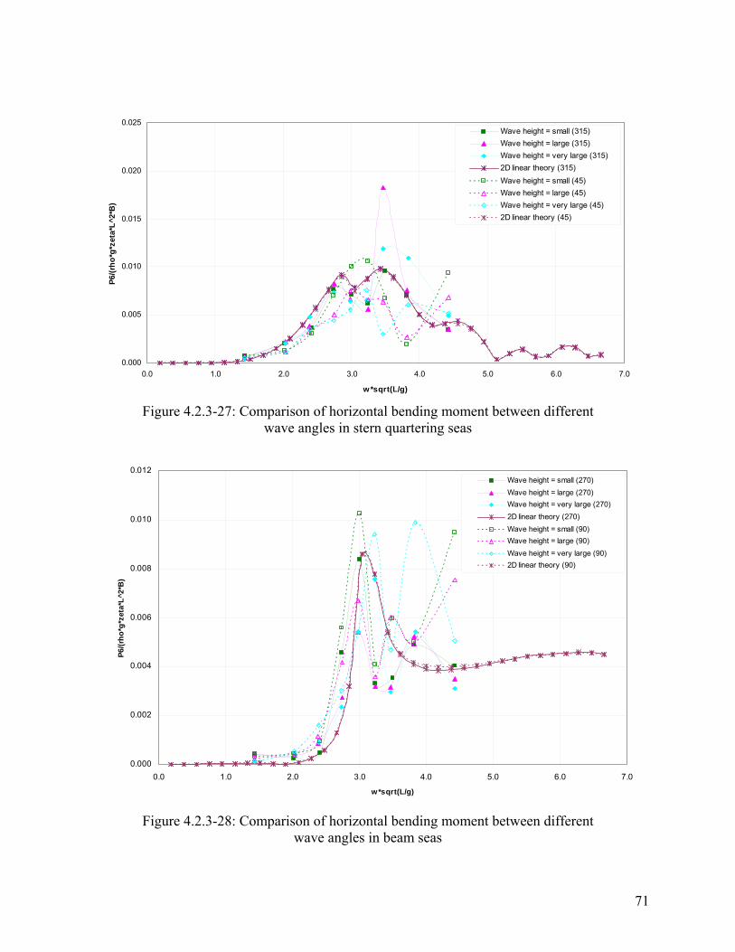
0.000
0.005
0.010
0.015
0.020
0.025
0.0 1.0 2.0 3.0 4.0 5.0 6.0 7.0
w*sqrt(L/g)
P6/(r
ho*g
*zet
a*L^
2*B
)
Wave height = small (315)Wave height = large (315)Wave height = very large (315)2D linear theory (315)Wave height = small (45)Wave height = large (45)Wave height = very large (45)2D linear theory (45)
Figure 4.2.3-27: Comparison of horizontal bending moment between different
wave angles in stern quartering seas
0.000
0.002
0.004
0.006
0.008
0.010
0.012
0.0 1.0 2.0 3.0 4.0 5.0 6.0 7.0
w*sqrt(L/g)
P6/(r
ho*g
*zet
a*L^
2*B
)
Wave height = small (270)Wave height = large (270)Wave height = very large (270)2D linear theory (270)Wave height = small (90)Wave height = large (90)Wave height = very large (90)2D linear theory (90)
Figure 4.2.3-28: Comparison of horizontal bending moment between different
wave angles in beam seas
71
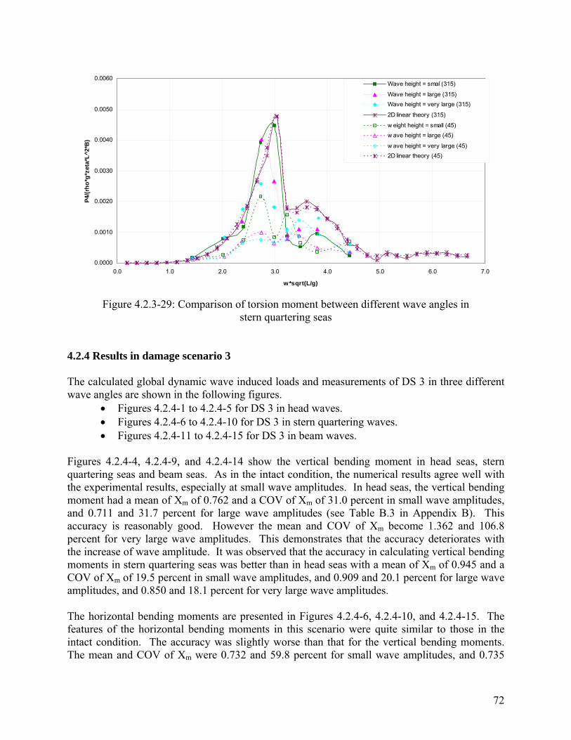
0.0000
0.0010
0.0020
0.0030
0.0040
0.0050
0.0060
0.0 1.0 2.0 3.0 4.0 5.0 6.0 7
w*sqrt(L/g)
P4/(r
ho*g
*zet
a*L^
2*B
)
.0
Wave height = smal (315)
Wave height = large (315)Wave height = very large (315)
2D linear theory (315)
w eight height = small (45)w ave height = large (45)
w ave height = very large (45)2D linear theory (45)
Figure 4.2.3-29: Comparison of torsion moment between different wave angles in
stern quartering seas
4.2.4 Results in damage scenario 3 The calculated global dynamic wave induced loads and measurements of DS 3 in three different wave angles are shown in the following figures.
• Figures 4.2.4-1 to 4.2.4-5 for DS 3 in head waves. • Figures 4.2.4-6 to 4.2.4-10 for DS 3 in stern quartering waves. • Figures 4.2.4-11 to 4.2.4-15 for DS 3 in beam waves.
Figures 4.2.4-4, 4.2.4-9, and 4.2.4-14 show the vertical bending moment in head seas, stern quartering seas and beam seas. As in the intact condition, the numerical results agree well with the experimental results, especially at small wave amplitudes. In head seas, the vertical bending moment had a mean of Xm of 0.762 and a COV of Xm of 31.0 percent in small wave amplitudes, and 0.711 and 31.7 percent for large wave amplitudes (see Table B.3 in Appendix B). This accuracy is reasonably good. However the mean and COV of Xm become 1.362 and 106.8 percent for very large wave amplitudes. This demonstrates that the accuracy deteriorates with the increase of wave amplitude. It was observed that the accuracy in calculating vertical bending moments in stern quartering seas was better than in head seas with a mean of Xm of 0.945 and a COV of Xm of 19.5 percent in small wave amplitudes, and 0.909 and 20.1 percent for large wave amplitudes, and 0.850 and 18.1 percent for very large wave amplitudes. The horizontal bending moments are presented in Figures 4.2.4-6, 4.2.4-10, and 4.2.4-15. The features of the horizontal bending moments in this scenario were quite similar to those in the intact condition. The accuracy was slightly worse than that for the vertical bending moments. The mean and COV of Xm were 0.732 and 59.8 percent for small wave amplitudes, and 0.735
72

and 49.7 percent for large wave amplitudes, and 0.894 and 41.1 percent for large wave amplitudes. The torsion moments are shown in Figures 4.2.4-3, 4.2.4-8, and 4.2.4-13. The torsion moments in head seas are insignificant, while the features of the torsion moments in stern quartering seas and beam seas in this scenario were quite similar to those in the intact condition. The mean and COV of Xm in stern quartering seas were 1.145 and 133.0 percent for small wave amplitudes, and 0.925 and 130.0 percent for large wave amplitudes, and 0.790 and 110.9 percent for very large wave amplitudes. The accuracy of the torsion moment prediction was poor, especially in the resonant region. Head waves
0.00
0.01
0.02
0.03
0.04
0.05
0.06
0.07
0.0 1.0 2.0 3.0 4.0 5.0 6.0 7.0
w*sqrt(L/g)
P2/(r
ho*g
*zet
a*L*
B)
Wave height = small
Wave height = large
w ave height=very large
2D linear theroy w ith estimatedTCG
Figure 4.2.4-1: Horizontal shear force RAO in DS 3 in head waves
73
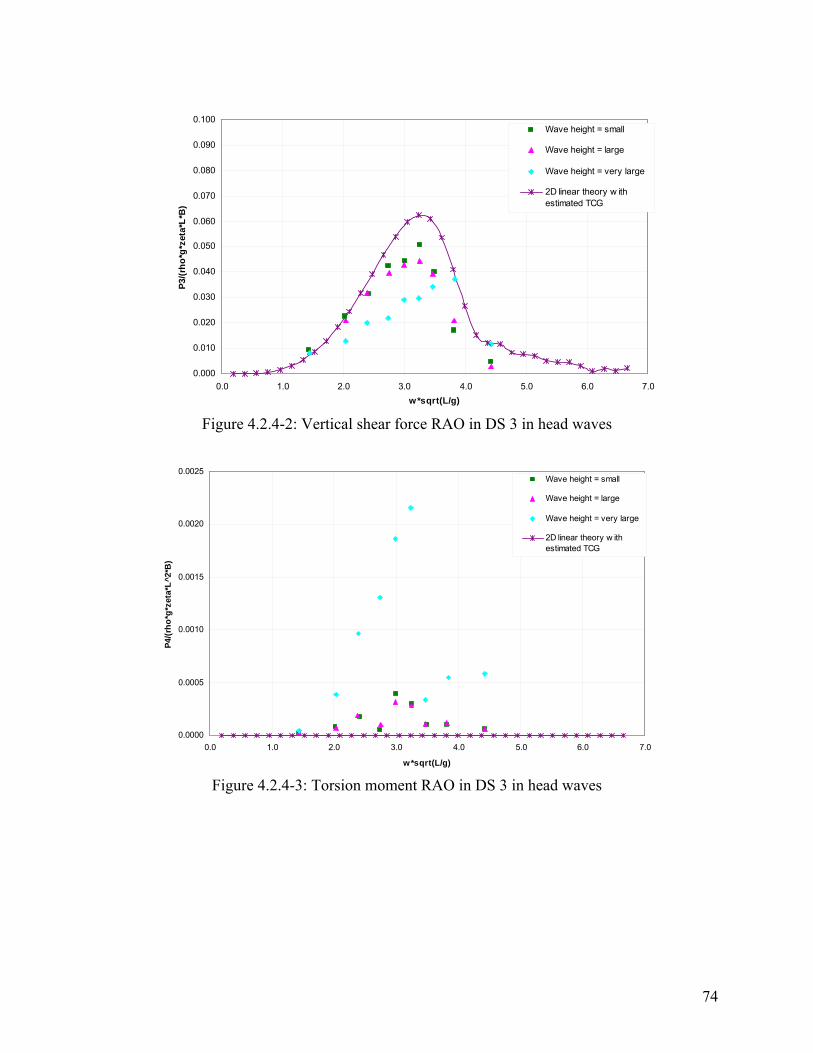
0.000
0.010
0.020
0.030
0.040
0.050
0.060
0.070
0.080
0.090
0.100
0.0 1.0 2.0 3.0 4.0 5.0 6.0 7.0w*sqrt(L/g)
P3/(r
ho*g
*zet
a*L*
B)
Wave height = small
Wave height = large
Wave height = very large
2D linear theory w ithestimated TCG
Figure 4.2.4-2: Vertical shear force RAO in DS 3 in head waves
0.0000
0.0005
0.0010
0.0015
0.0020
0.0025
0.0 1.0 2.0 3.0 4.0 5.0 6.0 7.0
w*sqrt(L/g)
P4/(r
ho*g
*zet
a*L^
2*B
)
Wave height = small
Wave height = large
Wave height = very large
2D linear theory w ithestimated TCG
Figure 4.2.4-3: Torsion moment RAO in DS 3 in head waves
74

0.000
0.005
0.010
0.015
0.020
0.0 1.0 2.0 3.0 4.0 5.0 6.0 7.0w*sqrt(L/g)
P5/(r
ho*g
*zet
a*L^
2*B
)
Wave height = small
Wave height = large
Wave height = very large
2D linear theory w ithestimated TCG)
Figure 4.2.4-4: Vertical bending moment RAO in DS 3 in head waves
0.000
0.002
0.004
0.006
0.008
0.010
0.012
0.0 1.0 2.0 3.0 4.0 5.0 6.0 7
w*sqrt(L/g)
P6/(r
ho*g
*zet
a*L^
2*B
)
.0
Wave height = small
Wave height = large
Wave height = very large
2D linear theory w ithestimated TCG
Figure 4.2.4-5: Horizontal bending moment RAO in DS 3 in head waves
75

Stern quartering waves
0.00
0.01
0.02
0.03
0.04
0.05
0.06
0.07
0.08
0.09
0.10
0.0 1.0 2.0 3.0 4.0 5.0 6.0 7.0
w*sqrt(L/g)
P2/(r
ho*g
*zet
a*L*
B)
Wave height = small
Wave height = large
w ave height=very large
2D linear theroy w ith estimatedTCG
Figure 4.2.4-6: Horizontal shear force RAO in DS 3 in stern quartering waves
0.000
0.010
0.020
0.030
0.040
0.050
0.060
0.0 1.0 2.0 3.0 4.0 5.0 6.0 7.0w*sqrt(L/g)
P3/(r
ho*g
*zet
a*L*
B)
Wave height = small
Wave height = large
Wave height = very large
2D linear theory w ithestimated TCG
Figure 4.2.4-7: Vertical shear force RAO in DS 3 in stern quartering waves
76

0.0000
0.0010
0.0020
0.0030
0.0040
0.0050
0.0060
0.0070
0.0080
0.0090
0.0 1.0 2.0 3.0 4.0 5.0 6.0 7.0
w*sqrt(L/g)
P4/(r
ho*g
*zet
a*L^
2*B
)Wave height = small
Wave height = large
Wave height = very large
2D linear theory w ith estimatedTCG
Figure 4.2.4-8: Torsion moment RAO in DS 3 in stern quartering waves
0.000
0.005
0.010
0.015
0.020
0.0 1.0 2.0 3.0 4.0 5.0 6.0 7.0w*sqrt(L/g)
P5/(r
ho*g
*zet
a*L^
2*B
)
Wave height = small
Wave height = large
Wave height = very large
2D linear theory w ithestimated TCG
Figure 4.2.4-9: Vertical bending moment RAO in DS 3 in stern quartering waves
77

0.000
0.002
0.004
0.006
0.008
0.010
0.012
0.0 1.0 2.0 3.0 4.0 5.0 6.0 7.
w*sqrt(L/g)
P6/(r
ho*g
*zet
a*L^
2*B
)
0
Wave height = small
Wave height = large
Wave height = very large
2D linear theory w ithestimated TCG
Figure 4.2.4-10: Horizontal bending moment RAO in DS 3 in stern quartering waves
Beam waves
0.00
0.01
0.02
0.03
0.04
0.05
0.06
0.07
0.0 1.0 2.0 3.0 4.0 5.0 6.0 7.0
w*sqrt(L/g)
P2/(r
ho*g
*zet
a*L*
B)
Wave height = small
Wave height = large
w ave height=very large
2D linear theroy w ithestimated TCG
Figure 4.2.4-11: Horizontal shear force RAO in DS 3 in beam waves
78

0.000
0.010
0.020
0.030
0.040
0.050
0.060
0.0 1.0 2.0 3.0 4.0 5.0 6.0 7.0w*sqrt(L/g)
P3/(r
ho*g
*zet
a*L*
B)
Wave height = small
Wave height = large
Wave height = very large
2D linear theory w ith estimatedTCG
Figure 4.2.4-12: Vertical shear force RAO in DS 3 in beam waves
0.0000
0.0020
0.0040
0.0060
0.0080
0.0100
0.0120
0.0140
0.0 1.0 2.0 3.0 4.0 5.0 6.0 7.0
w*sqrt(L/g)
P4/(r
ho*g
*zet
a*L^
2*B
)
Wave height = small
Wave height = large
Wave height = very large
2D linear theory w ithestimated TCG
Figure 4.2.4-13: Torsion moment RAO in DS 3 in beam waves
79
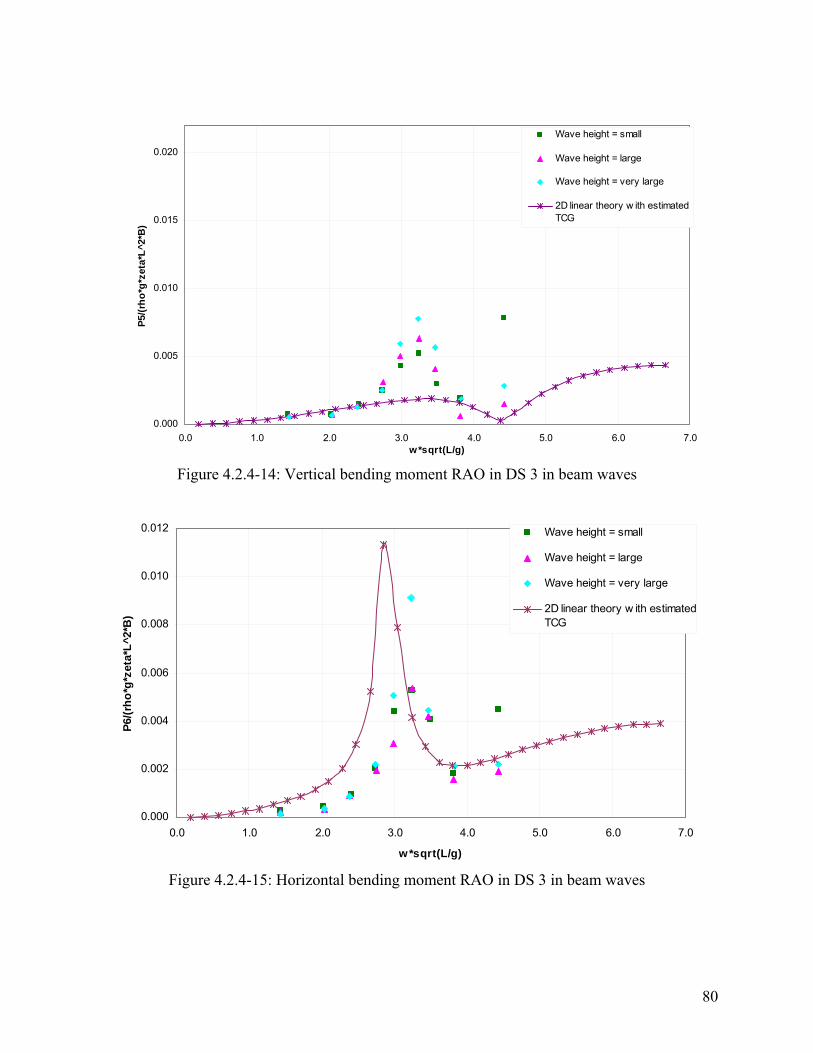
0.000
0.005
0.010
0.015
0.020
0.0 1.0 2.0 3.0 4.0 5.0 6.0 7.0w*sqrt(L/g)
P5/(r
ho*g
*zet
a*L^
2*B
)Wave height = small
Wave height = large
Wave height = very large
2D linear theory w ith estimatedTCG
Figure 4.2.4-14: Vertical bending moment RAO in DS 3 in beam waves
0.000
0.002
0.004
0.006
0.008
0.010
0.012
0.0 1.0 2.0 3.0 4.0 5.0 6.0 7.0
w*sqrt(L/g)
P6/(r
ho*g
*zet
a*L^
2*B
)
Wave height = small
Wave height = large
Wave height = very large
2D linear theory w ith estimatedTCG
Figure 4.2.4-15: Horizontal bending moment RAO in DS 3 in beam waves
80
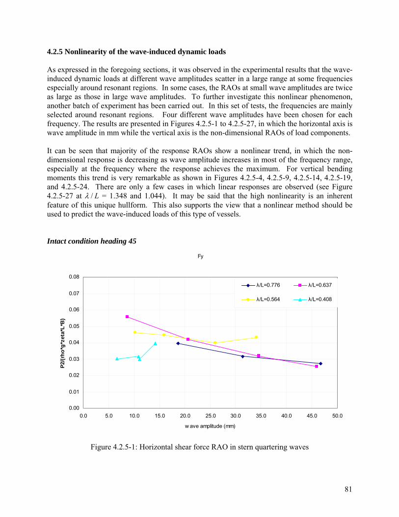
4.2.5 Nonlinearity of the wave-induced dynamic loads As expressed in the foregoing sections, it was observed in the experimental results that the wave-induced dynamic loads at different wave amplitudes scatter in a large range at some frequencies especially around resonant regions. In some cases, the RAOs at small wave amplitudes are twice as large as those in large wave amplitudes. To further investigate this nonlinear phenomenon, another batch of experiment has been carried out. In this set of tests, the frequencies are mainly selected around resonant regions. Four different wave amplitudes have been chosen for each frequency. The results are presented in Figures 4.2.5-1 to 4.2.5-27, in which the horizontal axis is wave amplitude in mm while the vertical axis is the non-dimensional RAOs of load components. It can be seen that majority of the response RAOs show a nonlinear trend, in which the non-dimensional response is decreasing as wave amplitude increases in most of the frequency range, especially at the frequency where the response achieves the maximum. For vertical bending moments this trend is very remarkable as shown in Figures 4.2.5-4, 4.2.5-9, 4.2.5-14, 4.2.5-19, and 4.2.5-24. There are only a few cases in which linear responses are observed (see Figure 4.2.5-27 at L/λ = 1.348 and 1.044). It may be said that the high nonlinearity is an inherent feature of this unique hullform. This also supports the view that a nonlinear method should be used to predict the wave-induced loads of this type of vessels. Intact condition heading 45
Fy
0.00
0.01
0.02
0.03
0.04
0.05
0.06
0.07
0.08
0.0 5.0 10.0 15.0 20.0 25.0 30.0 35.0 40.0 45.0 50.0
w ave amplitude (mm)
P2/(r
ho*g
*zet
a*L*
B)
λ/L=0.776 λ/L=0.637
λ/L=0.564 λ/L=0.408
Figure 4.2.5-1: Horizontal shear force RAO in stern quartering waves
81

Fz
0.00
0.01
0.02
0.03
0.04
0.05
0.06
0.07
0.08
0.0 5.0 10.0 15.0 20.0 25.0 30.0 35.0 40.0 45.0 50.0
w ave amplitude (mm)
P3/(r
ho*g
*zet
a*L*
B)
λ/L=0.776 λ/L=0.637
λ/L=0.564 λ/L=0.408
Figure 4.2.5-2: Vertical shear force RAO in stern quartering waves
Mx
0.0000
0.0005
0.0010
0.0015
0.0020
0.0025
0.0030
0.0035
0.0040
0.0045
0.0050
0.0 5.0 10.0 15.0 20.0 25.0 30.0 35.0 40.0 45.0 50.0
w ave amplitudes (mm)
P4/(r
ho*g
*zet
a*L^
2*B
)
λ/L=0.776 λ/L=0.637
λ/L=0.564 λ/L=0.408
Figure 4.2.5-3: Torsion moment RAO in stern quartering waves
82

My
0.00
0.01
0.02
0.02
0.03
0.04
0.0 5.0 10.0 15.0 20.0 25.0 30.0 35.0 40.0 45.0 50.0
w ave amplitude (mm)
P5/(r
ho*g
*zet
a*L*
B)
λ/L=0.776 λ/L=0.637
λ/L=0.564 λ/L=0.408
Figure 4.2.5-4: Vertical bending moment RAO in stern quartering waves
Mz
0.000
0.002
0.004
0.006
0.008
0.010
0.012
0.014
0.0 5.0 10.0 15.0 20.0 25.0 30.0 35.0 40.0 45.0 50.0
w ave amplitudes (mm)
P6/(r
ho*g
*zet
a*L^
2*B
)
λ/L=0.776 λ/L=0.637
λ/L=0.564 λ/L=0.408
Figure 4.2.5-5: Horizontal bending moment RAO in stern quartering waves
83

Intact condition heading 135
Fy
0.00
0.01
0.02
0.03
0.04
0.05
0.06
0.07
0.08
0.0 10.0 20.0 30.0 40.0 50.0 60.0
w ave amplitude (mm)
P2/(r
ho*g
*zet
a*L*
B)
λ/L=0.776 λ/L=0.637
λ/L=0.564 λ/L=0.408
λ/L=0.308
Figure 4.2.5-6: Horizontal shear force RAO in bow quartering waves
Fz
0.00
0.01
0.02
0.03
0.04
0.05
0.06
0.07
0.08
0.0 10.0 20.0 30.0 40.0 50.0 60.0
w ave amplitude (mm)
P3/(r
ho*g
*zet
a*L*
B)
λ/L=0.776 λ/L=0.637
λ/L=0.564 λ/L=0.408
λ/L=0.308
Figure 4.2.5-7: Vertical shear force RAO in bow quartering waves
84
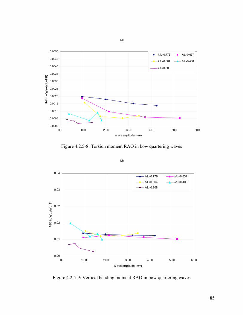
Mx
0.0000
0.0005
0.0010
0.0015
0.0020
0.0025
0.0030
0.0035
0.0040
0.0045
0.0050
0.0 10.0 20.0 30.0 40.0 50.0 60.0
w ave amplitudes (mm)
P4/(r
ho*g
*zet
a*L^
2*B
)
λ/L=0.776 λ/L=0.637
λ/L=0.564 λ/L=0.408
λ/L=0.308
Figure 4.2.5-8: Torsion moment RAO in bow quartering waves
My
0.00
0.01
0.02
0.02
0.03
0.04
0.0 10.0 20.0 30.0 40.0 50.0 60.0
w ave amplitude (mm)
P5/(r
ho*g
*zet
a*L*
B)
λ/L=0.776 λ/L=0.637
λ/L=0.564 λ/L=0.408
λ/L=0.308
Figure 4.2.5-9: Vertical bending moment RAO in bow quartering waves
85
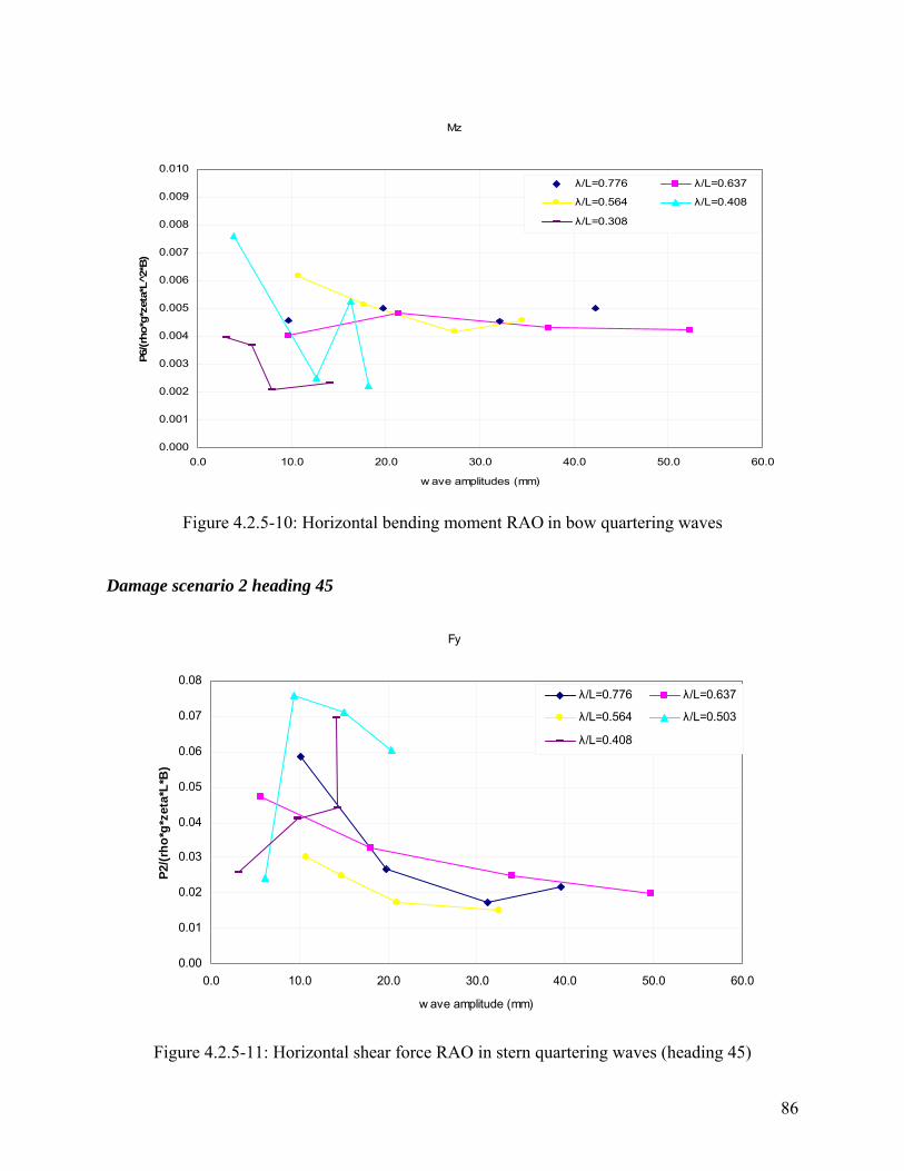
Mz
0.000
0.001
0.002
0.003
0.004
0.005
0.006
0.007
0.008
0.009
0.010
0.0 10.0 20.0 30.0 40.0 50.0 60.0
w ave amplitudes (mm)
P6/(r
ho*g
*zet
a*L
2*B
)
λ/L=0.776 λ/L=0.637
λ/L=0.564 λ/L=0.408
λ/L=0.308
Figure 4.2.5-10: Horizontal bending moment RAO in bow quartering waves
Damage scenario 2 heading 45
Fy
0.00
0.01
0.02
0.03
0.04
0.05
0.06
0.07
0.08
0.0 10.0 20.0 30.0 40.0 50.0 60.0
w ave amplitude (mm)
P2/(r
ho*g
*zet
a*L*
B)
λ/L=0.776 λ/L=0.637
λ/L=0.564 λ/L=0.503
λ/L=0.408
Figure 4.2.5-11: Horizontal shear force RAO in stern quartering waves (heading 45)
86

Fz
0.00
0.01
0.02
0.03
0.04
0.05
0.06
0.07
0.08
0.0 10.0 20.0 30.0 40.0 50.0 60.0
w ave amplitude (mm)
P3/(r
ho*g
*zet
a*L*
B)
λ/L=0.776 λ/L=0.637λ/L=0.564 λ/L=0.503λ/L=0.408
Figure 4.2.5-12: Vertical shear force RAO in stern quartering waves (heading 45)
Mx
0.0000
0.0005
0.0010
0.0015
0.0020
0.0025
0.0030
0.0035
0.0040
0.0045
0.0050
0.0 10.0 20.0 30.0 40.0 50.0 60.0
w ave amplitudes (mm)
P4/(r
ho*g
*zet
a*L^
2*B
)
λ/L=0.776 λ/L=0.637
λ/L=0.564 λ/L=0.503
λ/L=0.408
Figure 4.2.5-13: Torsion RAO in stern quartering waves (heading 45)
87

My
0.00
0.01
0.02
0.02
0.03
0.04
0.0 10.0 20.0 30.0 40.0 50.0 60.0
w ave amplitude (mm)
P5/(r
ho*g
*zet
a*L*
B)
λ/L=0.776 λ/L=0.637λ/L=0.564 λ/L=0.503λ/L=0.408
Figure 4.2.5-14: Vertical bending moment RAO in stern quartering waves (heading 45)
Mz
0.000
0.002
0.004
0.006
0.008
0.010
0.012
0.014
0.0 10.0 20.0 30.0 40.0 50.0 60.0
w ave amplitudes (mm)
P6/(r
ho*g
*zet
a*L^
2*B
)
λ/L=0.776 λ/L=0.637
λ/L=0.564 λ/L=0.503
λ/L=0.408
Figure 4.2.5-15: Horizontal bending moment RAO in stern quartering waves (heading 45)
88

Damage scenario 2 heading 315
Fy
0.00
0.02
0.04
0.06
0.08
0.10
0.12
0.14
0.16
0.0 5.0 10.0 15.0 20.0 25.0 30.0 35.0 40.0 45.0 50.0
w ave amplitude (mm)
P2/(r
ho*g
*zet
a*L*
B)
λ/L=0.776 λ/L=0.637
λ/L=0.408
Figure 4.2.5-16: Horizontal shear force RAO in stern quartering waves (heading 315)
Fz
0.00
0.01
0.02
0.03
0.04
0.05
0.06
0.07
0.08
0.0 5.0 10.0 15.0 20.0 25.0 30.0 35.0 40.0 45.0 50.0
w ave amplitude (mm)
P3/(r
ho*g
*zet
a*L*
B)
λ/L=0.776 λ/L=0.637
λ/L=0.408
Figure 4.2.5-17: Vertical shear force RAO in stern quartering waves (heading 315)
89

Mz
0.000
0.002
0.004
0.006
0.008
0.010
0.012
0.014
0.0 5.0 10.0 15.0 20.0 25.0 30.0 35.0 40.0 45.0 50.0
w ave amplitudes (mm)
P6/(r
ho*g
*zet
a*L^
2*B
)
λ/L=0.776 λ/L=0.637
λ/L=0.408
Figure 4.2.5-18: Torsion moment RAO in stern quartering waves (heading 315)
My
0.00
0.01
0.02
0.02
0.03
0.04
0.0 5.0 10.0 15.0 20.0 25.0 30.0 35.0 40.0 45.0 50.0
w ave amplitude (mm)
P5/(r
ho*g
*zet
a*L*
B)
λ/L=0.776 λ/L=0.637
λ/L=0.408
Figure 4.2.5-19: Vertical bending moment RAO in stern quartering waves (heading 315)
90

Mz
0.000
0.002
0.004
0.006
0.008
0.010
0.012
0.014
0.0 5.0 10.0 15.0 20.0 25.0 30.0 35.0 40.0 45.0 50.0
w ave amplitudes (mm)
P6/(r
ho*g
*zet
a*L^
2*B
)λ/L=0.776 λ/L=0.637
λ/L=0.408
Figure 4.2.5-20: Horizontal bending moment RAO in stern quartering waves (heading 315)
Damage scenario 3 heading 45
Fy
0.00
0.01
0.02
0.03
0.04
0.05
0.06
0.07
0.08
0.0 10.0 20.0 30.0 40.0 50.0 60.0
w ave amplitude (mm)
P2/(r
ho*g
*zet
a*L*
B)
λ/L=0.637 λ/L=0.564
λ/L=0.503 λ/L=0.408
Figure 4.2.5-21: Horizontal shear force RAO in stern quartering waves
91

Fz
0.00
0.01
0.02
0.03
0.04
0.05
0.06
0.07
0.08
0.0 10.0 20.0 30.0 40.0 50.0 60.0
w ave amplitude (mm)
P3/(r
ho*g
*zet
a*L*
B)
λ/L=0.637 λ/L=0.564
λ/L=0.503 λ/L=0.408
Figure 4.2.5-22: Vertical shear force RAO in stern quartering waves
Mx
0.0000
0.0005
0.0010
0.0015
0.0020
0.0025
0.0030
0.0035
0.0040
0.0045
0.0050
0.0 10.0 20.0 30.0 40.0 50.0 60.0
w ave amplitudes (mm)
P4/(r
ho*g
*zet
a*L^
2*B
)
λ/L=0.637 λ/L=0.564
λ/L=0.503 λ/L=0.408
Figure 4.2.5-23: Torsion moment RAO in stern quartering waves
92

My
0.00
0.01
0.02
0.02
0.03
0.04
0.0 10.0 20.0 30.0 40.0 50.0 60.0
w ave amplitude (mm)
P5/(r
ho*g
*zet
a*L*
B)λ/L=0.637 λ/L=0.564
λ/L=0.503 λ/L=0.408
Figure 4.2.5-24: Vertical bending moment RAO in stern quartering waves
Mz
0.000
0.002
0.004
0.006
0.008
0.010
0.012
0.014
0.0 10.0 20.0 30.0 40.0 50.0 60.0
w ave amplitudes (mm)
P6/(r
ho*g
*zet
a*L^
2*B
)
λ/L=0.637 λ/L=0.564
λ/L=0.503 λ/L=0.408
Figure 4.2.5-25: Horizontal bending moment RAO in stern quartering waves
93

Damage scenario 3 heading 180
Fz
0.00
0.01
0.02
0.03
0.04
0.05
0.06
0.07
0.08
0.0 5.0 10.0 15.0 20.0 25.0 30.0 35.0 40.0 45.0
w ave amplitude (mm)
P3/(r
ho*g
*zet
a*L*
B)
λ/L=1.348 λ/L=1.044
λ/L=0.564 λ/L=0.503
λ/L=0.408
Figure 4.2.5-26: Vertical shear force RAO in head waves
My
0.00
0.01
0.02
0.02
0.03
0.04
0.0 5.0 10.0 15.0 20.0 25.0 30.0 35.0 40.0 45.0
w ave amplitude (mm)
P5/(r
ho*g
*zet
a*L*
B)
λ/L=1.348 λ/L=1.044
λ/L=0.564 λ/L=0.503
λ/L=0.408
Figure 4.2.5-27: Vertical bending moment RAO in head waves
94

4.3 Prediction of dynamic global wave loads using the 2-D nonlinear theory An in-house program, which is based on the 2-D nonlinear method presented in Chapter 2, has been used to calculate wave-induced loads in regular waves in this section in order to validate the nonlinear method and compare it with the 2-D linear method presented in the previous sections. For a given wave profile this method can calculate the dynamic responses in the time domain. The time series are then filtered and the responses in the frequency domain are obtained. Due to the nonlinearity in the responses, it is expected that the calculated RAOs in different wave amplitudes would be different, so two wave amplitudes, namely 2.0 and 2.5 metres, have been chosen to calculate the RAOs of wave-induced loads on the ship model at the cut. One of the advantages of using a nonlinear method is its ability to distinguish the difference between positive and negative amplitude of the responses, while the positive and negative amplitude in a linear method would be the same. For ships, for instance, the sagging bending moment is normally greater than the hogging bending moment, especially for destroyers. Therefore positive and negative responses are presented separately to show their difference in the following figures. Figures 4.3-1 to 4.3-34 compare the 2-D nonlinear results with the experimental results in the intact condition and damage scenario 2. Due to the limited capability of the wave maker, the waves generated in the towing tank can’t exactly match the wave amplitudes that were used in the theoretical calculations. Hence the “large” wave amplitudes in the experiment have been used to compare with the wave amplitude of 2m in theory, and “very large” wave amplitudes in the experiment have been used to compare with wave amplitude of 2.5m in theory. Only head seas and stern quartering seas are considered in this section because they are the critical headings for strength assessment. Horizontal bending moments and torsion moments in the intact condition were not discussed in this comparison, as they were almost zero in the numerical predictions. The sign conventions of dynamic force and moment on the transverse section of aft portion of the cut concerned are:
• Horizontal shear force is positive from starboard to port. • Upward vertical shear force is positive. • Anti-clockwise torsion moment is positive. • Positive vertical bending moment is hogging. • Horizontal bending moment is positive when its vector points upward.
Figure 4.3-3 shows the results for vertical bending moments in the intact condition in head waves with a wave height of 2 metres in the numerical calculations. Also presented in this figure are the results of the 2-D linear method so the relative accuracy of both linear and nonlinear methods can be observed. More details of the quantitative comparison of the 2-D nonlinear method with the experimental results can be seen in Table C.1 in Appendix C, in which the model uncertainties of the nonlinear method are presented. Close attention will be paid to the results at the frequencies of 2.37, 2.74, and 2.97 because the wave height in the tests at those frequencies was very near to 2.0 metres. The 2-D nonlinear results of the vertical bending moment agree reasonably well with the experimental results at some cases, such as positive amplitude at frequency 2.97 and negative amplitude at frequency 2.37. The values of Xm in those cases were 0.779 and 0.791 respectively. However the agreement was poor in some other cases, such as positive amplitude at frequency 2.37. The value of Xm in that case was 0.598. The mean and
95

COV of Xm were 0.910 and 63.3 percent for positive amplitude, and 1.280 and 102.6 percent for negative amplitude. Further investigation into the constituents of Xm has shown that there is a large value of 2.342 for positive amplitude and 4.771 for negative amplitude at low frequencies. This large value could distort the mean and COV especially when the total number of data points is only 9. In addition, the wave height in the test at this frequency was less than 0.7 metres, which was far away from 2.0 metres used in the numerical calculation. Hence caution needs to be applied if the model uncertainty factor is to be used. The results of the 2-D linear method fall in between the positive and negative amplitudes predicted by the 2-D nonlinear method in the resonant region, so the linear and nonlinear methods correlate fairly well in this condition. Overall, the performance of the 2-D nonlinear method was not satisfactory in this case. Figure 4.3-4 shows the results for vertical bending moments in the intact condition in head waves with a wave height of 2.5 metres in the numerical calculations. The features of this figure were quite similar to those of Figure 4.3-3. It should be pointed out that the majority of the experimental wave heights were not near the corresponding numerical wave height in this case. The mean and COV of Xm were 1.038 and 100.4 percent for positive amplitude and 0.671 and 30.1 percent for negative amplitude. Again the agreement between the 2-D nonlinear method and the tests was not desirable. Figure 4.3-9 shows the results for vertical bending moments in the intact condition in stern quartering seas with a wave height of 2.0 metres in the numerical calculations. Again, more attention will be paid to the results at the frequencies of 2.37, 2.74, and 2.97. Generally the 2-D nonlinear results of the vertical bending moment do not agree well with the experimental results except for one case, which was the negative amplitude at frequency 2.97 with a value of Xm of 0.862. The values of Xm in the two bad cases were 0.497 and 0.509 respectively. The mean and COV of Xm were 0.941 and 95.6 percent for positive amplitude, and 0.737 and 40.3 percent for negative amplitude. Figure 4.3-19 shows the results for vertical bending moments in damage scenario 2 in head waves with a wave height of 2 metres in the numerical calculations. For the same reason more attention will be paid to the results at the frequencies of 2.37, 2.74, and 2.97. The 2-D nonlinear results for the vertical bending moments agree reasonably well with the experimental results in some cases, such as positive amplitude at frequency 2.74 and negative amplitude at frequency 2.37. The values of Xm in those cases were 0.832 and 0.838 respectively as shown in Table C.2 in Appendix C. However the agreement was not satisfactory in some other cases, such as negative amplitude at frequencies 2.74 and 2.97, and positive amplitude at frequency 2.37. The values of Xm in those three cases were 0.599, 0.606 and 0.620 respectively. The mean and COV of Xm were 1.084 and 75.4 percent for positive amplitude, and 0.596 and 43.9 percent for negative amplitude. Further investigation into the constituents of Xm has shown that there is a very large value of 22.107 for positive amplitude and 17.572 for negative amplitude at a very low frequency of 1.435. This large value could distort the mean and COV especially when the total number of data points is only 9. In addition the wave height in the test was 1.148 metres, which was far away from 2.0 metres used in the numerical calculation at this low frequency. Hence caution needs to be applied if the model uncertainty factor is to be used.
96

The results for vertical bending moments in damage scenario 2 in stern quartering seas with a wave height of 2 metres in the numerical calculations are presented in Figure 4.3-29 and Table C.2 in Appendix C. As before the results at the frequencies of 2.37, 2.74, and 2.97 were under close scrutiny. The 2-D nonlinear results of the vertical bending moment agree reasonably well with the experimental results at some cases, such as positive amplitude at frequencies 2.37 and 2.97 and negative amplitude at frequency 2.97. The values of Xm in those cases were 0.862 and 0.914 respectively as shown in Table C.2 in Appendix C. However the agreement was poor in some other cases, such as negative amplitude at frequencies 2.37, and positive amplitude at frequency 2.74. The values of Xm in those two cases were 0.606 and 0.668 respectively. The mean and COV of Xm were 0.719 and 43.9 percent for positive amplitude, and 0.866 and 41.1 percent for negative amplitude. This is the best performance for vertical bending moment prediction. The horizontal bending moments in the intact condition in stern quartering seas with a wave height of 2 metres in the numerical calculations is presented in Figure 4.3-11 and Table C.1 in Appendix C. As before the results at the frequencies of 2.37, 2.74, and 2.97 were the main focus. The 2-D nonlinear results of the horizontal bending moment do not agree well with the experimental results at these frequencies. The values of Xm in those cases vary in a large range from 0.227 to 2.906 as shown in Table C.1 in Appendix C. The mean and COV of Xm were 1.357 and 110 percent for positive amplitude, and 0.528 and 60.9 percent for negative amplitude. It is interesting to note that both linear and nonlinear methods produce two peaks, but the predicted peaks did not match the peak that was measured in the tests. This seems the main reason for such a bad performance in the numerical predictions. Figure 4.3-31 shows the results for horizontal bending moments in damage scenario 2 in stern quartering seas with a wave height of 2 metres in the numerical calculations. For the same reason the results at the frequencies of 2.37, 2.74, and 2.97 were the focus. The 2-D nonlinear results of the horizontal bending moment agree reasonably well with the experimental results in some cases, such as positive amplitude at frequency 2.37 and 2.74. The values of Xm in those cases were 0.842 and 1.147 respectively as shown in Table C.2 in Appendix C. However the agreement was not satisfactory in some other cases, such as negative amplitude at all frequencies, and positive amplitude at frequency 2.97. The values of Xm in those four cases were 0.208, 0.342, 0.428 and 1.897, respectively. The mean and COV of Xm were 1.109 and 60.3 percent for positive amplitude, and 0.602 and 91.9 percent for negative amplitude. The torsion moments in the intact condition in stern quartering seas with a wave height of 2 metres in the numerical calculations is presented in Figure 4.3-13 and Table C.1 in Appendix C. As before the results at the frequencies of 2.37, 2.74, and 2.97 were the main focus. The 2-D nonlinear results of the torsion moment agree well with the experimental results at some frequencies but not the others. The mean and COV of Xm were 0.4955 and 105.5 percent for positive amplitude, and 0.489 and 47.2 percent for negative amplitude. It is interesting to note that the nonlinear method correctly predicted the peak responses, but the agreement at other frequencies were so bad so that the mean and COV of Xm are quite unsatisfactory.
97

Figure 4.3-33 shows the results for the torsion moments in damage scenario 2 in stern quartering seas with a wave height of 2 metres in the numerical calculations. The 2-D nonlinear results for the torsion moment do not agree well with the experimental results at almost all the frequencies. As shown in Table C.2 in Appendix C the mean and COV of Xm were 0.130 and 85.1 percent for positive amplitude, and 0.343 and 82.8 percent for negative amplitude. Basically, the experimental results were much smaller than the predicted responses. In summary, the 2-D nonlinear method does not produce satisfactory results for vertical bending moments, horizontal bending moments and torsion moments. Although this conclusion is largely based on the analysis of the results from 2 metres wave height, it was equally applicable to the results of 2.5 metres wave height as shown in the corresponding figures and Table C.1 and C.2 in Appendix C. Again, the predictions of torsion moments are the worst among the three components of the wave-induced loads, while the predictions of vertical bending moments have a similar level of accuracy to those of horizontal bending moments. The nonlinear method tends to produce better results at the resonant frequencies than at the other frequencies. However, it should be pointed out that the measured wave heights were not equal to 2.0 metres, which was used in the numerical calculations at most frequencies so that caution has to be applied when the mean and COV of Xm are used to judge the accuracy of the method. Intact Condition Head seas
0.000
0.010
0.020
0.030
0.040
0.050
0.060
0.070
0.080
0.090
0.100
0.0 1.0 2.0 3.0 4.0 5.0 6.0 7
w*sqrt(L/g)
P3/(r
ho*g
*zet
a*L*
B)
.0
2D linear theory w ith estimated TCG
Exp. large w ave amp positive
Exp. large w ave amp negative
Non-linear theory 2m positive
Non-linear theory 2m negative
Figure 4.3-1: Dynamic vertical shear force RAO
in head seas (heading 180), theory ζ = 2m
98

0.000
0.020
0.040
0.060
0.080
0.100
0.120
0.140
0.0 1.0 2.0 3.0 4.0 5.0 6.0 7.0
w*sqrt(L/g)
P3/(r
ho*g
*zet
a*L*
B)
2D linear theory w ith estimated TCG
Exp.very large w ave amp positive
Exp.very large w ave amp negative
Non-linear theory 2.5m positive
Non-linear theory 2.5m negative
Figure 4.3-2: Dynamic vertical shear force RAO
in head seas (heading 180), theory ζ = 2.5m
0.000
0.005
0.010
0.015
0.020
0.025
0.030
0.035
0.040
0.0 1.0 2.0 3.0 4.0 5.0 6.0 7.0w*sqrt(L/g)
P5/(r
ho*g
*zet
a*L^
2*B
)
2D linear theory w ith estimated TCG
Exp. large w ave amp positive
Exp. large w ave amp negative
Non-linear theory 2m positive
Non-linear theory 2m negative
Figure 4.3-3: Dynamic vertical bending moment RAO
in head seas (heading 180), theory ζ = 2m
99
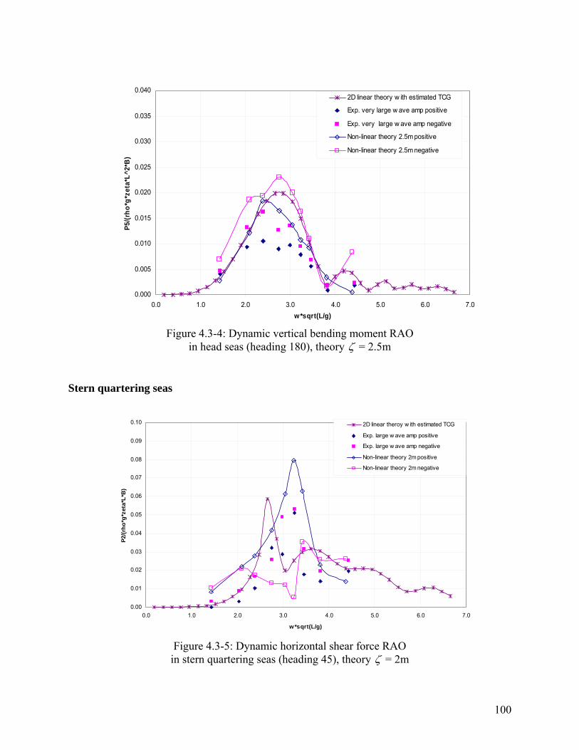
0.000
0.005
0.010
0.015
0.020
0.025
0.030
0.035
0.040
0.0 1.0 2.0 3.0 4.0 5.0 6.0 7.0w*sqrt(L/g)
P5/(r
ho*g
*zet
a*L^
2*B
)
2D linear theory w ith estimated TCG
Exp. very large w ave amp positive
Exp. very large w ave amp negative
Non-linear theory 2.5m positive
Non-linear theory 2.5m negative
Figure 4.3-4: Dynamic vertical bending moment RAO
in head seas (heading 180), theory ζ = 2.5m Stern quartering seas
0.00
0.01
0.02
0.03
0.04
0.05
0.06
0.07
0.08
0.09
0.10
0.0 1.0 2.0 3.0 4.0 5.0 6.0 7.0
w*sqrt(L/g)
P2/(r
ho*g
*zet
a*L*
B)
2D linear theroy w ith estimated TCG
Exp. large w ave amp positive
Exp. large w ave amp negative
Non-linear theory 2m positive
Non-linear theory 2m negative
Figure 4.3-5: Dynamic horizontal shear force RAO
in stern quartering seas (heading 45), theory ζ = 2m
100

0.00
0.01
0.02
0.03
0.04
0.05
0.06
0.07
0.08
0.09
0.10
0.0 1.0 2.0 3.0 4.0 5.0 6.0 7.0
w*sqrt(L/g)
P2/(r
ho*g
*zet
a*L*
B)
2D linear theroy w ith estimated TCG
Exp. very large w ave amp positive
Exp.very large w ave amp negative
Non-linear theory 2.5m positive
Non-linear theory 2.5m negative
Figure 4.3-6: Dynamic horizontal shear force RAO
in stern quartering seas (heading 45), theory ζ = 2.5m
0.000
0.010
0.020
0.030
0.040
0.050
0.060
0.070
0.080
0.090
0.100
0.0 1.0 2.0 3.0 4.0 5.0 6.0 7
w*sqrt(L/g)
P3/(r
ho*g
*zet
a*L*
B)
.0
2D linear theory w ith estimated TCG
Exp. large w ave amp positive
Exp. large w ave amp negative
Non-linear theory 2m positive
Non-linear theory 2m negative
Figure 4.3-7: Dynamic vertical shear force RAO
in stern quartering seas (heading 45), theory ζ = 2m
101

-0.010
0.010
0.030
0.050
0.070
0.090
0.110
0.130
0.150
0.0 1.0 2.0 3.0 4.0 5.0 6.0
w*sqrt(L/g)
P3/(r
ho*g
*zet
a*L*
B)
7.0
2D linear theory w ith estimated TCG
Exp.very large w ave amp positive
Exp.very large w ave amp negative
Non-linear theory 2.5m positive
Non-linear theory 2.5m negative
Figure 4.3-8: Dynamic vertical shear force RAO
in stern quartering seas (heading 45), theory ζ = 2.5m
0.000
0.005
0.010
0.015
0.020
0.025
0.030
0.035
0.040
0.0 1.0 2.0 3.0 4.0 5.0 6.0 7.0w*sqrt(L/g)
P5/(r
ho*g
*zet
a*L^
2*B
)
2D linear theory w ith estimated TCG
Exp. large w ave amp positive
Exp. large w ave amp negative
Non-linear theory 2m positive
Non-linear theory 2m negative
Figure 4.3-9: Dynamic vertical bending moment RAO in stern quartering seas (heading 45), theory ζ = 2m
102
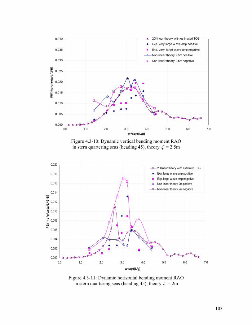
0.000
0.005
0.010
0.015
0.020
0.025
0.030
0.035
0.040
0.0 1.0 2.0 3.0 4.0 5.0 6.0 7.0w*sqrt(L/g)
P5/(r
ho*g
*zet
a*L^
2*B
)
2D linear theory w ith estimated TCG
Exp. very large w ave amp positive
Exp. very large w ave amp negative
Non-linear theory 2.5m positive
Non-linear theory 2.5m negative
Figure 4.3-10: Dynamic vertical bending moment RAO in stern quartering seas (heading 45), theory ζ = 2.5m
0.000
0.002
0.004
0.006
0.008
0.010
0.012
0.014
0.016
0.018
0.020
0.0 1.0 2.0 3.0 4.0 5.0 6.0 7.0
w*sqrt(L/g)
P6/(r
ho*g
*zet
a*L^
2*B
)
2D linear theory w ith estimated TCGExp. large w ave amp positiveExp. large w ave amp negativeNon-linear theory 2m positiveNon-linear theory 2m negative
Figure 4.3-11: Dynamic horizontal bending moment RAO
in stern quartering seas (heading 45), theory ζ = 2m
103

0.000
0.002
0.004
0.006
0.008
0.010
0.012
0.014
0.016
0.018
0.020
0.0 1.0 2.0 3.0 4.0 5.0 6.0 7.0
w*sqrt(L/g)
P6/(r
ho*g
*zet
a*L^
2*B
)2D linear theory w ith estimated TCGExp. very large w ave amp positiveExp. very large w ave amp negativeNon-linear theory 2.5m positiveNon-linear theory 2.5m negative
Figure 4.3-12: Dynamic horizontal bending moment RAO
in stern quartering seas (heading 45), theory ζ = 2.5m
0.0000
0.0020
0.0040
0.0060
0.0080
0.0100
0.0120
0.0140
0.0 1.0 2.0 3.0 4.0 5.0 6.0 7.0
w*sqrt(L/g)
P4/(r
ho*g
*zet
a*L^
2*B
)
2D linear theory w ith estimated TCGExp. large w ave amp positiveExp. large w ave amp negativeNon-linear theory 2m positiveNon-linear theory 2m negative
Figure 4.3-13: Dynamic torsion moment RAO
in stern quartering seas (heading 45), theory ζ = 2m
104

0.0000
0.0020
0.0040
0.0060
0.0080
0.0100
0.0120
0.0140
0.0 1.0 2.0 3.0 4.0 5.0 6.0 7.0
w*sqrt(L/g)
P4/(r
ho*g
*zet
a*L^
2*B
)
2D linear theory w ith estimated TCGExp. very large w ave amp positiveExp. very large w ave amp negativeNon-linear theory 2.5m positiveNon-linear theory 2.5m negative
Figure 4.3-14: Dynamic torsion moment RAO
in stern quartering seas (heading 45), theory ζ = 2.5m Damage Scenario 2 Head Seas
0.00
0.01
0.02
0.03
0.04
0.05
0.06
0.07
0.08
0.09
0.10
0.0 1.0 2.0 3.0 4.0 5.0 6.0 7.0
w*sqrt(L/g)
P2/(r
ho*g
*zet
a*L*
B)
2D linear theroy w ith estimated TCG
Exp. large w ave amp positive
Exp. large w ave amp negative
Non-linear theory 2m positive
Non-linear theory 2m negative
Figure 4.3-15: Dynamic horizontal shear force RAO
in head seas (heading 180), theory ζ = 2m
105

0.00
0.01
0.02
0.03
0.04
0.05
0.06
0.07
0.08
0.09
0.10
0.0 1.0 2.0 3.0 4.0 5.0 6.0 7
w*sqrt(L/g)
P2/(r
ho*g
*zet
a*L*
B)
.0
2D linear theroy w ith estimated TCG
Exp. very large w ave amp positive
Exp.very large w ave amp negative
Non-linear theory 2.5m positive
Non-linear theory 2.5m negative
Figure 4.3-16: Dynamic horizontal shear force RAO
in head seas (heading 180), theory ζ = 2.5m
0.000
0.010
0.020
0.030
0.040
0.050
0.060
0.070
0.080
0.090
0.100
0.0 1.0 2.0 3.0 4.0 5.0 6.0 7.0
w*sqrt(L/g)
P3/(r
ho*g
*zet
a*L*
B)
2D linear theory w ith estimated TCG
Exp. large w ave amp positive
Exp. large w ave amp negative
Non-linear theory 2m positive
Non-linear theory 2m negative
Figure 4.3-17: Dynamic vertical shear force RAO
in head seas (heading 180), theory ζ = 2m
106

-0.010
0.010
0.030
0.050
0.070
0.090
0.110
0.130
0.150
0.0 1.0 2.0 3.0 4.0 5.0 6.0 7
w*sqrt(L/g)
P3/(r
ho*g
*zet
a*L*
B)
.0
2D linear theory w ith estimated TCG
Exp.very large w ave amp positive
Exp.very large w ave amp negative
Non-linear theory 2.5m positive
Non-linear theory 2.5m negative
Figure 4.3-18: Dynamic vertical shear force RAO
in head seas (heading 180), theory ζ = 2.5m
0.000
0.005
0.010
0.015
0.020
0.025
0.030
0.035
0.040
0.0 1.0 2.0 3.0 4.0 5.0 6.0 7.0w*sqrt(L/g)
P5/(r
ho*g
*zet
a*L^
2*B
)
2D linear theory w ith estimated TCG
Exp. large w ave amp positive
Exp. large w ave amp negative
Non-linear theory 2m positive
Non-linear theory 2m negative
Figure 4.3-19: Dynamic vertical bending moment RAO
in head seas (heading 180), theory ζ = 2m
107

0.000
0.005
0.010
0.015
0.020
0.025
0.030
0.035
0.040
0.0 1.0 2.0 3.0 4.0 5.0 6.0 7.0w*sqrt(L/g)
P5/(r
ho*g
*zet
a*L^
2*B
)
2D linear theory w ith estimated TCG
Exp. very large w ave amp positive
Exp. very large w ave amp negative
Non-linear theory 2.5m positive
Non-linear theory 2.5m negative
Figure 4.3-20: Dynamic vertical bending moment RAO
in head seas (heading 180), theory ζ = 2.5m
0.000
0.001
0.002
0.003
0.004
0.005
0.006
0.007
0.008
0.009
0.010
0.0 1.0 2.0 3.0 4.0 5.0 6.0 7.0
w*sqrt(L/g)
P6/(r
ho*g
*zet
a*L^
2*B
)
2D linear theory w ith estimated TCGExp. large w ave amp positiveExp. large w ave amp negativeNon-linear theory 2m positiveNon-linear theory 2m positive
Figure 4.3-21: Dynamic horizontal bending moment RAO
in head seas (heading 180), theory ζ = 2m
108

0.000
0.001
0.002
0.003
0.004
0.005
0.006
0.007
0.008
0.009
0.010
0.0 1.0 2.0 3.0 4.0 5.0 6.0 7.
w*sqrt(L/g)
P6/(r
ho*g
*zet
a*L^
2*B
)
0
2D linear theory w ith estimated TCGExp. very large w ave amp positiveExp. very large w ave amp negativeNon-linear theory 2.5m positiveNon-linear theory 2.5m positive
Figure 4.3-22: Dynamic horizontal bending moment RAO
in head seas (heading 180), theory ζ = 2.5m
0.0000
0.0010
0.0020
0.0030
0.0040
0.0050
0.0060
0.0 1.0 2.0 3.0 4.0 5.0 6.0 7.
w*sqrt(L/g)
P4/(r
ho*g
*zet
a*L^
2*B
)
0
2D linear theory w ith estimated TCGExp. large w ave amp positiveExp. large w ave amp negativeNon-linear theory 2m positiveNon-linear theory 2m negative
Figure 4.3-23: Dynamic torsion moment RAO
in head seas (heading 180), theory ζ = 2m
109
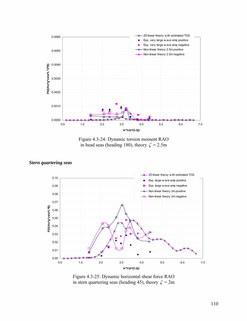
0.0000
0.0010
0.0020
0.0030
0.0040
0.0050
0.0060
0.0 1.0 2.0 3.0 4.0 5.0 6.0 7.0
w*sqrt(L/g)
P4/(r
ho*g
*zet
a*L^
2*B
)
2D linear theory w ith estimated TCGExp. very large w ave amp positiveExp. very large w ave amp negativeNon-linear theory 2.5m positiveNon-linear theory 2.5m negative
Figure 4.3-24: Dynamic torsion moment RAO in head seas (heading 180), theory ζ = 2.5m
Stern quartering seas
0.00
0.01
0.02
0.03
0.04
0.05
0.06
0.07
0.08
0.09
0.10
0.0 1.0 2.0 3.0 4.0 5.0 6.0 7.0
w*sqrt(L/g)
P2/(r
ho*g
*zet
a*L*
B)
2D linear theroy w ith estimated TCG
Exp. large w ave amp positive
Exp. large w ave amp negative
Non-linear theory 2m positive
Non-linear theory 2m negative
Figure 4.3-25: Dynamic horizontal shear force RAO in stern quartering seas (heading 45), theory ζ = 2m
110

0.00
0.01
0.02
0.03
0.04
0.05
0.06
0.07
0.08
0.09
0.10
0.0 1.0 2.0 3.0 4.0 5.0 6.0 7.0
w*sqrt(L/g)
P2/(r
ho*g
*zet
a*L*
B)
2D linear theroy w ith estimated TCG
Exp. very large w ave amp positive
Exp.very large w ave amp negative
Non-linear theory 2.5m positive
Non-linear theory 2.5m negative
Figure 4.3-26: Dynamic horizontal shear force RAO
in stern quartering seas (heading 45), theory ζ = 2.5m
0.00
0.01
0.02
0.03
0.04
0.05
0.06
0.07
0.08
0.09
0.10
0.0 1.0 2.0 3.0 4.0 5.0 6.0 7.0
w*sqrt(L/g)
P2/(r
ho*g
*zet
a*L*
B)
2D linear theroy w ith estimated TCG
Exp. large w ave amp positive
Exp. large w ave amp negative
Non-linear theory 2m positive
Non-linear theory 2m negative
Figure 4.3-27: Dynamic vertical shear force RAO
in stern quartering seas (heading 45), theory ζ = 2m
111
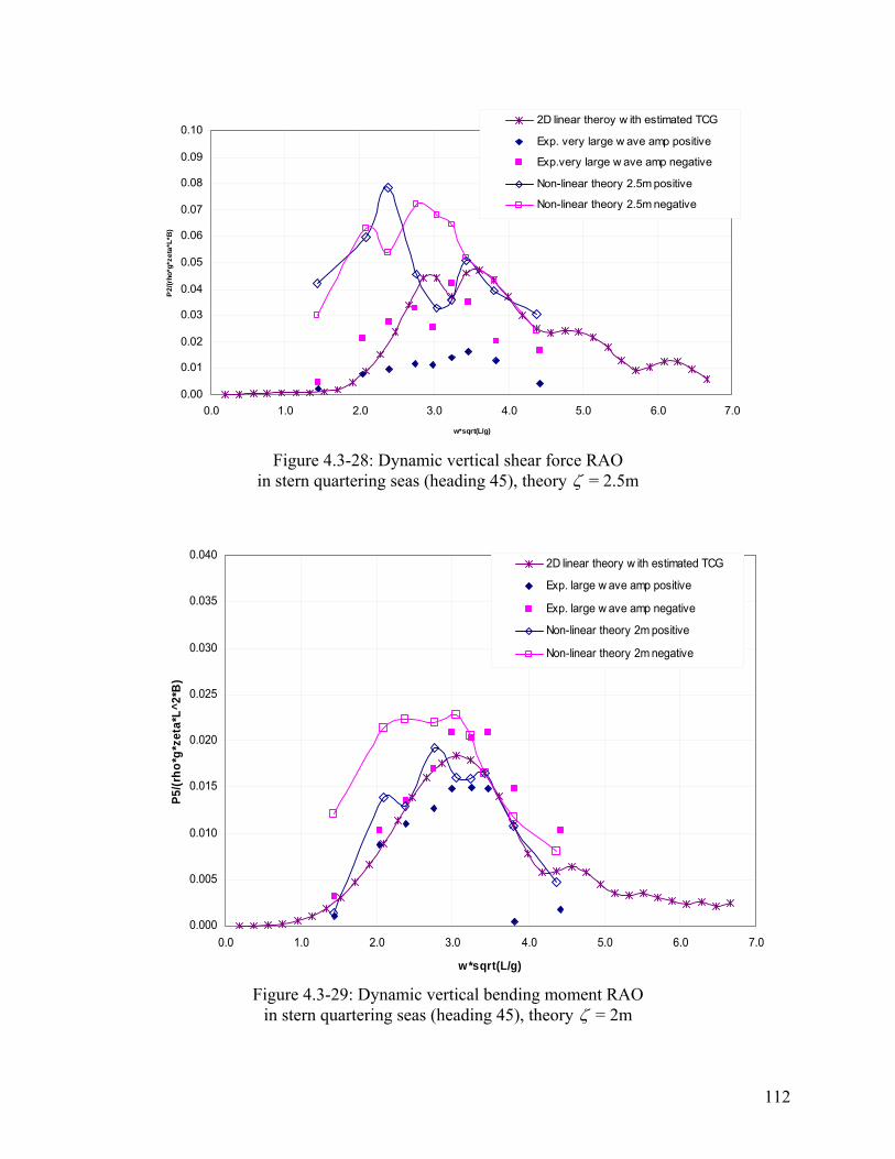
0.00
0.01
0.02
0.03
0.04
0.05
0.06
0.07
0.08
0.09
0.10
0.0 1.0 2.0 3.0 4.0 5.0 6.0 7.0
w*sqrt(L/g)
P2/
(rho
*g*z
eta*
L*B
)
2D linear theroy w ith estimated TCG
Exp. very large w ave amp positive
Exp.very large w ave amp negative
Non-linear theory 2.5m positive
Non-linear theory 2.5m negative
Figure 4.3-28: Dynamic vertical shear force RAO
in stern quartering seas (heading 45), theory ζ = 2.5m
0.000
0.005
0.010
0.015
0.020
0.025
0.030
0.035
0.040
0.0 1.0 2.0 3.0 4.0 5.0 6.0 7.0
w*sqrt(L/g)
P5/(r
ho*g
*zet
a*L^
2*B
)
2D linear theory w ith estimated TCG
Exp. large w ave amp positive
Exp. large w ave amp negative
Non-linear theory 2m positive
Non-linear theory 2m negative
Figure 4.3-29: Dynamic vertical bending moment RAO
in stern quartering seas (heading 45), theory ζ = 2m
112
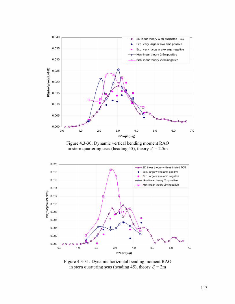
0.000
0.005
0.010
0.015
0.020
0.025
0.030
0.035
0.040
0.0 1.0 2.0 3.0 4.0 5.0 6.0 7
w*sqrt(L/g)
P5/(r
ho*g
*zet
a*L^
2*B
)
.0
2D linear theory w ith estimated TCG
Exp. very large w ave amp positive
Exp. very large w ave amp negative
Non-linear theory 2.5m positive
Non-linear theory 2.5m negative
Figure 4.3-30: Dynamic vertical bending moment RAO in stern quartering seas (heading 45), theory ζ = 2.5m
0.000
0.002
0.004
0.006
0.008
0.010
0.012
0.014
0.016
0.018
0.020
0.0 1.0 2.0 3.0 4.0 5.0 6.0 7.0
w*sqrt(L/g)
P6/(r
ho*g
*zet
a*L^
2*B
)
2D linear theory w ith estimated TCGExp. large w ave amp positiveExp. large w ave amp negativeNon-linear theory 2m positiveNon-linear theory 2m negative
Figure 4.3-31: Dynamic horizontal bending moment RAO
in stern quartering seas (heading 45), theory ζ = 2m
113

0.000
0.002
0.004
0.006
0.008
0.010
0.012
0.014
0.016
0.018
0.020
0.0 1.0 2.0 3.0 4.0 5.0 6.0 7.0
w*sqrt(L/g)
P6/(r
ho*g
*zet
a*L^
2*B
)2D linear theory w ith estimated TCGExp. very large w ave amp positiveExp. very large w ave amp negativeNon-linear theory 2.5m positiveNon-linear theory 2.5m negative
Figure 4.3-32: Dynamic horizontal bending moment RAO
in stern quartering seas (heading 45), theory ζ = 2.5m
0.0000
0.0020
0.0040
0.0060
0.0080
0.0100
0.0120
0.0140
0.0 1.0 2.0 3.0 4.0 5.0 6.0 7.
w*sqrt(L/g)
P4/(r
ho*g
*zet
a*L^
2*B
)
0
2D linear theory w ith estimated TCGExp. large w ave amp positiveExp. large w ave amp negativeNon-linear theory 2m positiveNon-linear theory 2m negative
Figure 4.3-33: Dynamic torsion moment RAO
in stern quartering seas (heading 45), theory ζ = 2m
114

0.0000
0.0020
0.0040
0.0060
0.0080
0.0100
0.0120
0.0140
0.0 1.0 2.0 3.0 4.0 5.0 6.0 7.0
w*sqrt(L/g)
P4/(r
ho*g
*zet
a*L^
2*B
)
2D linear theory w ith estimated TCGExp. very large w ave amp positiveExp. very large w ave amp negativeNon-linear theory 2.5m positiveNon-linear theory 2.5m negative
Figure 4.3-34: Dynamic torsion moment RAO
in stern quartering seas (heading 45), theory ζ = 2.5m
4.4 Model Uncertainties of the 2-D Linear and Nonlinear Method As mentioned in Section 2.1.5 model uncertainty is a very important source of uncertainty in the structural design process. Since a coefficient of variation (COV) of a typical strength prediction could be about 10 to 15 percent while a COV of wave-induced load prediction could be well above 30 percent, model uncertainty of wave-induced load prediction is a major uncertainty in structural strength assessment. Hence the model uncertainties of the 2-D linear method and 2-D nonlinear method were calculated by using Equation (2.1-34) in that section. Based on the observations in the previous sections, the accuracies of both linear and nonlinear methods are different for different load components. It would be interesting to quantitatively demonstrate this difference, so the model uncertainties are calculated separately for different load components. Conventional model uncertainties were only predicted for the intact condition, so it would be interesting to see how different the accuracy could be between the intact condition and the damaged conditions. A summary of model uncertainties of the 2-D linear method and nonlinear method for vertical bending moment, horizontal bending moment as well as torsion moment are shown in Tables 4.4-1 and 4.4-2, while the details of the model uncertainty calculations are presented in Appendices B and C.
)X( 1m
115

Table 4.4-1: Model uncertainties of the 2-D linear method )X( 1m
Design
Condition Load Heading Mean (S) COV (S) Mean (L) COV (L) Mean (V) COV (V)
180 0.8879 0.1926 0.7729 0.2446 0.7503 0.2743 VBM 45 1.0108 0.3194 0.9062 0.3760 0.9230 0.3374
135 0.8647 0.2462 0.8443 0.2714 0.8053 0.6931 180 small values ≈ 0 small values ≈ 0 small values ≈ 0
Intact HBM 45 1.1190 0.7045 1.0192 0.6962 1.0379 0.4842 135 0.7812 0.6730 0.9129 0.7361 0.9249 0.7063 180 small values ≈ 0 small values ≈ 0 small values ≈ 0 TM 45 0.9638 1.3586 0.8660 1.4997 1.0264 1.2835 135 0.5590 0.6027 0.9187 1.4778 1.0481 1.6661 180 0.7894 0.2698 0.7393 0.2145 0.7832 0.1834 VBM 45 1.0633 0.2818 0.9744 0.1884 1.0101 0.2284 315 0.9792 0.2991 1.0049 0.5182 0.9488 0.3998 180 small values ≈ 0 small values ≈ 0 small values ≈ 0
DS 2 HBM 45 1.1644 0.6721 0.9192 0.5960 0.8479 0.5020 315 1.0160 0.4230 1.1236 0.4450 1.1247 0.3217 180 small values ≈ 0 small values ≈ 0 small values ≈ 0 TM 45 0.6329 0.6414 0.4888 0.6754 0.5067 0.6093 315 0.8277 0.5260 0.8734 0.4568 0.9341 0.4567 VBM 180 0.7616 0.3104 0.7117 0.3173 1.3621 1.0684
DS 3 45 0.9452 0.1946 0.9094 0.2009 0.8502 0.1812 HBM 180 small values ≈ 0 small values ≈ 0 small values ≈ 0 45 0.7320 0.5978 0.7347 0.4969 0.8942 0.4106 TM 180 small values ≈ 0 small values ≈ 0 small values ≈ 0 45 1.1452 1.3305 0.9247 1.2999 0.7901 1.1095
In Table 4.4-1 Mean (S) and COV (S) stand for mean and COV for each load component in small wave amplitudes; Mean (L) and COV (L) stand for mean and COV for each load component in large wave amplitudes; Mean (V) and COV (V) stand for mean and COV for each load component in very large wave amplitudes; VBM is vertical bending moment; HBM is horizontal bending moment; TM is torsion moment. From Table 4.4-1 it is observed that the accuracy of the vertical bending moments is generally better than that of horizontal bending moments and torsion moments, and the accuracy for loads in head seas is much better than for those in stern quartering seas and beam seas. This could be mainly caused by the underwater hullform of the ship model with a small Cb compared with conventional ships. The COV of the horizontal bending moments is almost as twice as large as that of the vertical bending moments. The COV of the torsion moments is the largest of the three.
116
Because of the large difference in COV for different force components it is more rational to consider the model uncertainties for vertical bending moments, horizontal bending moments, and torsion moments separately in reliability analysis rather than using one combined model uncertainty for all the components. When the model uncertainties were calculated, the experimental results were assumed as the ‘real response’. However there were also uncertainties in the tests, but unfortunately it was very difficult to quantify them although much effort has been made to reduce these uncertainties. One of the uncertainties in the current experiment was the way to measure the wave profile in terms of wave height and wave period. Two wave probes were placed in the front of the ship model to measure the wave profile. Due to the effects of deflection of incident wave and radiation of the model’s motion, the recorded wave in the second wave probe, which was nearer to the model, was subject to the interference, so could not be used. Therefore the wave profile measured by the first wave probe, which was further away from the model, was used to calculate the RAOs. It is possible that the wave profile at the first wave probe was slightly different from the wave profile at the ship model. Due to the limited availability of the towing tank, it was not possible to correlate fully the wave profile at these two locations so that this difference could be considered in the calculations. The second uncertainty is caused by the mooring lines, which were attached to the fore and stern ends of the model, as mentioned in the previous sections. The mooring line could affect the model’s motion, although more on the low frequency motions and less on the wave frequency motions, and then wave-induced loads, especially the horizontal bending moments. However the forces in the mooring lines were not measured so that it was not possible to quantify the influence of the mooring lines on the horizontal bending moment. The third uncertainty was the measurement of the radius of gyration about the x-axis (i.e. for roll motion). The roll radius of gyration of the model was measured by the method presented in Bhattacharyya (1978). In this method, a bar with circular cross-section was attached to the deck panel in the longitudinal direction (i.e. along the x-axis). Although the deck was strong enough to seal the model and to keep the model waterproof during the tests in the towing tank, it was not stiff enough so that it deformed noticeably when the whole model was hanging beneath the attached bar during the swing test. Therefore the accuracy in the measured roll radius of gyration may not be very good. This may cause the inaccuracy in the calculations of the natural frequency of roll and torsion moments. The large COV in the torsion moments might be partly caused by this uncertainty. Table 4.4-2 presents the model uncertainties of the 2-D nonlinear method. In this table
• ‘mean (2m)+’ is the mean value of model uncertainty under 2m wave weight from the positive responses;
• ‘mean (2m)-’ is the mean value of model uncertainty under 2m wave weight from the negative responses;
• ‘COV (2m)+’ is the coefficient of variation of model uncertainty under 2m wave weight from the positive responses;
• ‘COV (2m)-’ is the coefficient of variation of model uncertainty under 2m wave weight from the negative responses;
117

118
• ‘mean (2.5m)+’ is the mean value of model uncertainty under 2.5m wave weight from the positive responses;
• ‘mean (2.5m)-’ is the mean value of model uncertainty under 2.5m wave weight from the negative responses;
• ‘COV (2.5m)+’ is the coefficient of variation of model uncertainty under 2.5m wave weight from the positive responses;
• ‘COV (2.5m)-’ is the coefficient of variation of model uncertainty under 2.5m wave weight from the negative responses;
• ‘mean +’ is mean value of the model uncertainty under both 2m and 2.5m wave weight from the positive responses;
• ‘mean -’ is the mean value of model uncertainty under both 2m and 2.5m wave weight from the negative responses;
• ‘COV +’ is the coefficient of variation of model uncertainty under both 2m and 2.5m wave weight from the positive responses; and
• ‘COV -’ is the coefficient of variation of model uncertainty under both 2m and 2.5m-wave weight from the negative responses.
Comparing the results in Tables 4.4-1 and 4.4-2, it can be seen that the 2-D linear method has a better mean and COV of Xm in the predictions of vertical bending moments and horizontal bending moments in both the intact condition and damage scenario 2 than the 2-D nonlinear method, and both 2-D the linear and nonlinear methods have produced unsatisfactory results in torsion moments. Based on the current results, it may be said that the 2-D linear method is more accurate than the nonlinear method. However the nonlinear method can distinguish the difference between the positive and negative responses, but linear methods can’t. This advantage of the nonlinear method is especially important for ships with small block coefficient, such as frigates etc. For a frigate the ratio of sagging bending moment to hogging bending moment could be as large as 1.78 (Clarke, 1986). In addition, hull girder strength in hogging is normally different from that in sagging. Therefore the nonlinear method is preferred. This slight preference of the nonlinear method was also based on another fact that the nonlinear method tends to produce better results in the resonant region than at other frequencies. Based on the current method for combining different load components, the accuracy in the resonant region is more important than that at other frequencies.

Table 4.4-2: Model uncertainties of the 2-D nonlinear method )X( 1m
Design
condition Load Headin
g mean (2m)
+
mean (2m)
-
COV (2m)
+
COV (2m)
-
mean (2.5m)
+
mean (2.5m)
-
COV (2.5m)
+
COV (2.5m)
-
mean +
mean -
COV +
COV -
VBM 180 0.9104 1.2802 0.6332 1.0255 1.0382 0.6711 1.0040 0.3009 0.9743 0.9757 0.8413 0.9876Intact 45 0.9416 0.7365 0.9562 0.4032 0.6408 0.7926 0.4354 0.5354 0.7912 0.7646 0.8404 0.4662
HBM 45 1.3567 0.5282 1.0998 0.6088 1.2072 0.5960 0.6585 0.7275 1.2820 0.5621 0.9067 0.6617 TM 45 0.4955 0.4893 1.0548 0.4721 0.6664 0.4748 0.7152 0.5393 0.5810 0.4821 0.8488 0.4910 VBM 180 1.0838 0.5955 0.7537 0.4385 1.0307 0.6507 0.5186 0.3490 1.0557 0.6247 0.6251 0.3802
DS 2 45 0.7186 0.8661 0.4387 0.4113 0.7765 0.8083 0.3288 0.4025 0.7475 0.8372 0.3744 0.3969 HBM 45 1.1085 0.6020 0.6034 0.9186 1.1479 0.5114 0.6758 0.8428 1.1282 0.5567 0.6231 0.8680 TM 45 0.1295 0.3429 0.8507 0.8275 0.1706 0.4445 0.6280 0.5335 0.1500 0.3937 0.7165 0.6579
119
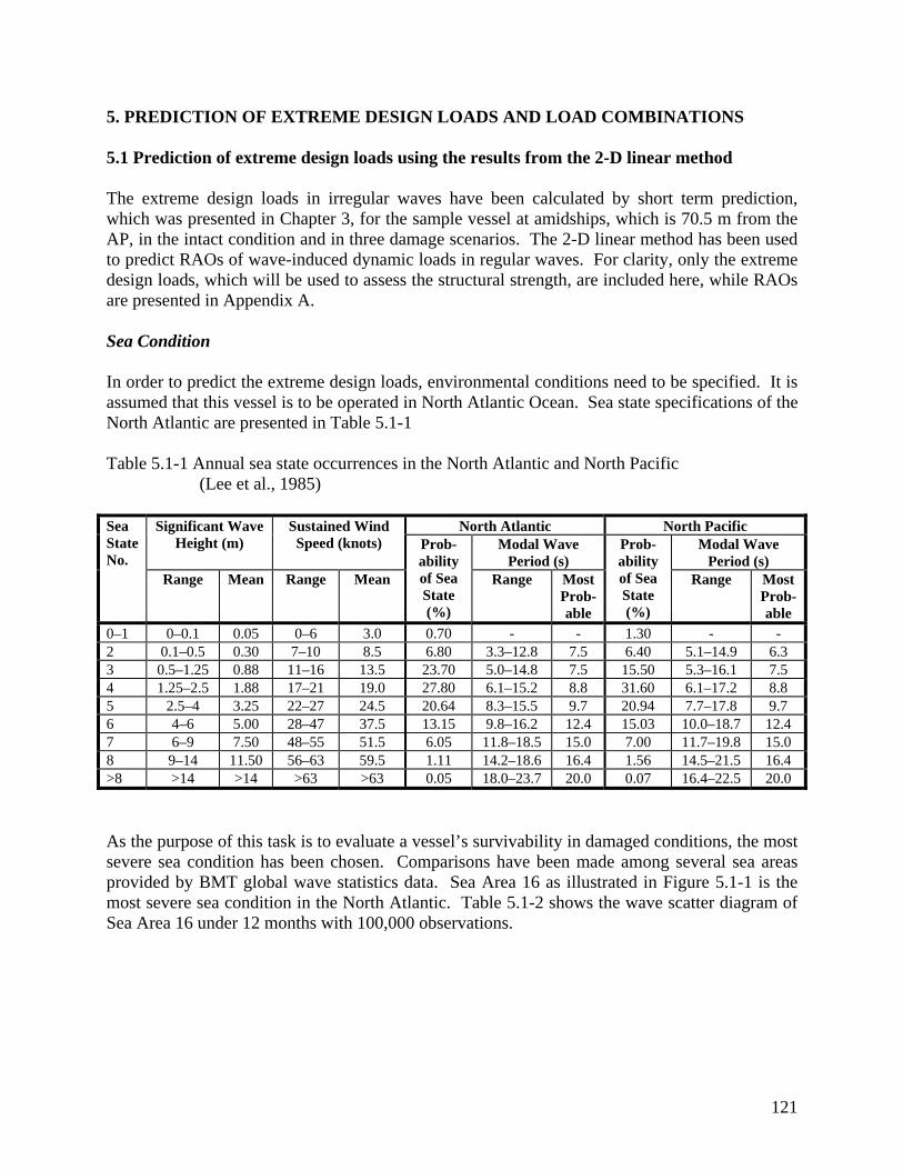
5. PREDICTION OF EXTREME DESIGN LOADS AND LOAD COMBINATIONS 5.1 Prediction of extreme design loads using the results from the 2-D linear method The extreme design loads in irregular waves have been calculated by short term prediction, which was presented in Chapter 3, for the sample vessel at amidships, which is 70.5 m from the AP, in the intact condition and in three damage scenarios. The 2-D linear method has been used to predict RAOs of wave-induced dynamic loads in regular waves. For clarity, only the extreme design loads, which will be used to assess the structural strength, are included here, while RAOs are presented in Appendix A. Sea Condition In order to predict the extreme design loads, environmental conditions need to be specified. It is assumed that this vessel is to be operated in North Atlantic Ocean. Sea state specifications of the North Atlantic are presented in Table 5.1-1 Table 5.1-1 Annual sea state occurrences in the North Atlantic and North Pacific
(Lee et al., 1985) Sea State No.
Significant Wave Height (m)
Sustained Wind Speed (knots)
North Atlantic North Pacific Prob-ability of Sea State (%)
Modal Wave Period (s)
Prob-ability of Sea State (%)
Modal Wave Period (s)
Range Mean Range Mean Range Most Prob-able
Range Most Prob-able
0–1 0–0.1 0.05 0–6 3.0 0.70 - - 1.30 - - 2 0.1–0.5 0.30 7–10 8.5 6.80 3.3–12.8 7.5 6.40 5.1–14.9 6.3 3 0.5–1.25 0.88 11–16 13.5 23.70 5.0–14.8 7.5 15.50 5.3–16.1 7.5 4 1.25–2.5 1.88 17–21 19.0 27.80 6.1–15.2 8.8 31.60 6.1–17.2 8.8 5 2.5–4 3.25 22–27 24.5 20.64 8.3–15.5 9.7 20.94 7.7–17.8 9.7 6 4–6 5.00 28–47 37.5 13.15 9.8–16.2 12.4 15.03 10.0–18.7 12.4 7 6–9 7.50 48–55 51.5 6.05 11.8–18.5 15.0 7.00 11.7–19.8 15.0 8 9–14 11.50 56–63 59.5 1.11 14.2–18.6 16.4 1.56 14.5–21.5 16.4 >8 >14 >14 >63 >63 0.05 18.0–23.7 20.0 0.07 16.4–22.5 20.0 As the purpose of this task is to evaluate a vessel’s survivability in damaged conditions, the most severe sea condition has been chosen. Comparisons have been made among several sea areas provided by BMT global wave statistics data. Sea Area 16 as illustrated in Figure 5.1-1 is the most severe sea condition in the North Atlantic. Table 5.1-2 shows the wave scatter diagram of Sea Area 16 under 12 months with 100,000 observations.
121

Figure 5.1-1 Location of Sea Area 16 (source: BMT) Table 5.1-2 Wave scatter diagram of Sea Area 16 in the North Atlantic (BMT)
Based on the information above, the significant wave height in each sea state and its corresponding zero crossing period in Sea Area 16 can be obtained as follows:
Hs (m) Zero crossing
period (s) Sea State 3 1.25 7.5 Sea State 4 2.5 8 Sea State 5 4 8.5 Sea State 6 6 9 Sea State 7 9 10
122
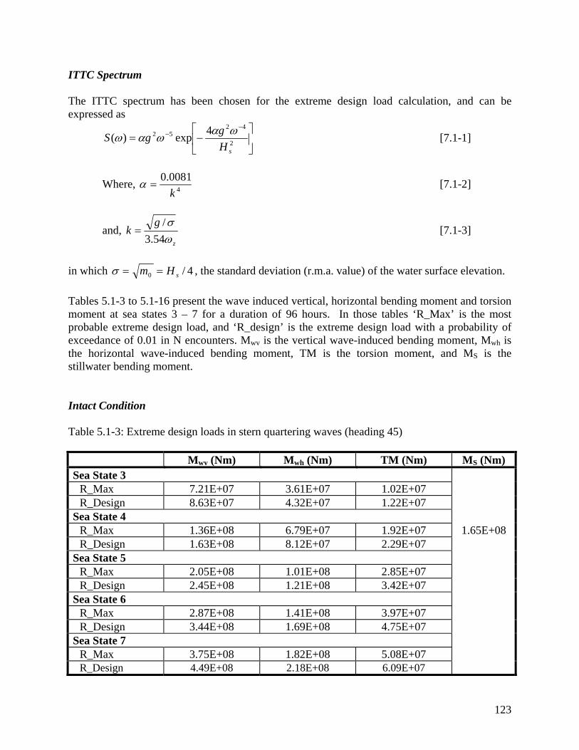
ITTC Spectrum The ITTC spectrum has been chosen for the extreme design load calculation, and can be expressed as
⎥⎦
⎤⎢⎣
⎡−=
−−
2
4252 4exp)(
sHggS ωαωαω [7.1-1]
Where, 4
0081.0k
=α [7.1-2]
and, z
gk
ωσ
54.3/
= [7.1-3]
in which 4/0 sHm ==σ , the standard deviation (r.m.a. value) of the water surface elevation. Tables 5.1-3 to 5.1-16 present the wave induced vertical, horizontal bending moment and torsion moment at sea states 3 – 7 for a duration of 96 hours. In those tables ‘R_Max’ is the most probable extreme design load, and ‘R_design’ is the extreme design load with a probability of exceedance of 0.01 in N encounters. Mwv is the vertical wave-induced bending moment, Mwh is the horizontal wave-induced bending moment, TM is the torsion moment, and MS is the stillwater bending moment. Intact Condition Table 5.1-3: Extreme design loads in stern quartering waves (heading 45) Mwv (Nm) Mwh (Nm) TM (Nm) MS (Nm) Sea State 3
R_Max 7.21E+07 3.61E+07 1.02E+07 R_Design 8.63E+07 4.32E+07 1.22E+07
Sea State 4 R_Max 1.36E+08 6.79E+07 1.92E+07 1.65E+08 R_Design 1.63E+08 8.12E+07 2.29E+07
Sea State 5 R_Max 2.05E+08 1.01E+08 2.85E+07 R_Design 2.45E+08 1.21E+08 3.42E+07
Sea State 6 R_Max 2.87E+08 1.41E+08 3.97E+07 R_Design 3.44E+08 1.69E+08 4.75E+07
Sea State 7 R_Max 3.75E+08 1.82E+08 5.08E+07 R_Design 4.49E+08 2.18E+08 6.09E+07
123

Table 5.1-4: Extreme design loads in head waves (heading 180) Mwv (Nm) Mwh (Nm) TM (Nm) MS (Nm) Sea State 3
R_Max 8.92E+07 1.13E+02 4.18E+00 R_Design 1.07E+08 1.35E+02 5.02E+00
Sea State 4 R_Max 1.74E+08 2.22E+02 8.21E+00 1.65E+08 R_Design 2.09E+08 2.66E+02 9.85E+00
Sea State 5 R_Max 2.69E+08 3.44E+02 1.28E+01 R_Design 3.23E+08 4.13E+02 1.54E+01
Sea State 6 R_Max 3.86E+08 4.97E+02 1.87E+01 R_Design 4.63E+08 5.96E+02 2.24E+01
Sea State 7 R_Max 5.22E+08 6.76E+02 2.65E+01 R_Design 6.26E+08 8.12E+02 3.18E+01
Table 5.1-5: Extreme design loads in beam waves (heading 90) Mwv (Nm) Mwh (Nm) TM (Nm) MS (Nm) Sea State 3
R_Max 1.01E+07 2.41E+07 1.52E+07 R_Design 1.20E+07 2.88E+07 1.82E+07
Sea State 4 R_Max 1.90E+07 4.45E+07 2.81E+07 1.65E+08 R_Design 2.27E+07 5.32E+07 3.36E+07
Sea State 5 R_Max 2.86E+07 6.57E+07 4.14E+07 R_Design 3.42E+07 7.85E+07 4.95E+07
Sea State 6 R_Max 4.05E+07 9.07E+07 5.69E+07 R_Design 4.84E+07 1.08E+08 6.81E+07
Sea State 7 R_Max 5.39E+07 1.16E+08 7.18E+07 R_Design 6.44E+07 1.38E+08 8.59E+07
124

Damage Scenario 1 Table 5.1-6: Extreme design loads in stern quartering waves (heading 45) Mwv (Nm) Mwh (Nm) TM (Nm) MS (Nm) Sea State 3
R_Max 7.48E+07 3.82E+07 8.14E+06 R_Design 8.95E+07 4.57E+07 9.74E+06
Sea State 4 R_Max 1.42E+08 7.12E+07 1.53E+07 5.51E+07 R_Design 1.70E+08 8.52E+07 1.83E+07
Sea State 5 R_Max 2.14E+08 1.06E+08 2.28E+07 R_Design 2.57E+08 1.27E+08 2.72E+07
Sea State 6 R_Max 3.02E+08 1.47E+08 3.17E+07 R_Design 3.62E+08 1.76E+08 3.79E+07
Sea State 7 R_Max 3.97E+08 1.88E+08 4.06E+07 R_Design 4.75E+08 2.25E+08 4.87E+07
Table 5.1-7: Extreme design loads in head waves (heading 180) Mwv (Nm) Mwh (Nm) TM (Nm) MS (Nm) Sea State 3
R_Max 9.26E+07 1.07E+02 1.05E+01 R_Design 1.11E+08 1.28E+02 1.25E+01
Sea State 4 R_Max 1.82E+08 2.12E+02 2.08E+01 5.51E+07 R_Design 2.18E+08 2.54E+02 2.49E+01
Sea State 5 R_Max 2.82E+08 3.30E+02 3.30E+01 R_Design 3.38E+08 3.95E+02 3.96E+01
Sea State 6 R_Max 4.06E+08 4.77E+02 4.91E+01 R_Design 4.87E+08 5.72E+02 5.90E+01
Sea State 7 R_Max 5.51E+08 6.51E+02 7.22E+01 R_Design 6.61E+08 7.82E+02 8.68E+01
125

Table 5.1-8: Extreme design loads in beam waves Mwv (Nm) Mwh (Nm) TM (Nm) MS (Nm) Sea State 3
R_Max 9.09E+06 2.14E+07 1.39E+07 R_Design 1.08E+07 2.56E+07 1.66E+07
Sea State 4 R_Max 1.62E+07 3.88E+07 2.54E+07 5.51E+07 R_Design 1.92E+07 4.63E+07 3.03E+07
Sea State 5 R_Max 2.32E+07 5.62E+07 3.70E+07 R_Design 2.75E+07 6.71E+07 4.42E+07
Sea State 6 R_Max 3.13E+07 7.65E+07 5.06E+07 R_Design 3.72E+07 9.13E+07 6.05E+07
Sea State 7 R_Max 3.87E+07 9.52E+07 6.33E+07 R_Design 4.59E+07 1.14E+08 7.57E+07
Damage Scenario 2 Table 5.1-9: Extreme design loads in stern quartering waves (heading 45) Mwv (Nm) Mwh (Nm) TM (Nm) MS (Nm) Sea State 3
R_Max 7.71E+07 3.59E+07 1.01E+07 R_Design 9.23E+07 4.29E+07 1.21E+07
Sea State 4 R_Max 1.47E+08 6.65E+07 1.94E+07 3.75E+07 R_Design 1.76E+08 7.95E+07 2.32E+07
Sea State 5 R_Max 2.24E+08 9.82E+07 2.95E+07 R_Design 2.68E+08 1.17E+08 3.53E+07
Sea State 6 R_Max 3.17E+08 1.36E+08 4.18E+07 R_Design 3.79E+08 1.62E+08 5.01E+07
Sea State 7 R_Max 4.20E+08 1.72E+08 5.55E+07 R_Design 5.03E+08 2.06E+08 6.65E+07
126

Table 5.1-10: Extreme design loads in head waves Mwv (Nm) Mwh (Nm) TM (Nm) MS (Nm) Sea State 3
R_Max 9.79E+07 6.79E+05 1.85E+05 R_Design 1.17E+08 8.12E+05 2.21E+05
Sea State 4 R_Max 1.93E+08 1.27E+06 3.56E+05 3.75E+07 R_Design 2.31E+08 1.52E+06 4.27E+05
Sea State 5 R_Max 3.00E+08 1.89E+06 5.45E+05 R_Design 3.60E+08 2.25E+06 6.53E+05
Sea State 6 R_Max 4.33E+08 2.62E+06 7.78E+05 R_Design 5.19E+08 3.14E+06 9.32E+05
Sea State 7 R_Max 5.90E+08 3.37E+06 1.04E+06 R_Design 7.09E+08 4.03E+06 1.25E+06
Table 5.1-11: Extreme design loads in beam waves (heading 90) Mwv (Nm) Mwh (Nm) TM (Nm) MS (Nm) Sea State 3
R_Max 2.53E+07 1.98E+07 1.64E+06 R_Design 3.01E+07 2.35E+07 1.94E+06
Sea State 4 R_Max 4.54E+07 3.55E+07 2.90E+06 3.75E+07 R_Design 5.41E+07 4.23E+07 3.44E+06
Sea State 5 R_Max 6.56E+07 5.11E+07 4.13E+06 R_Design 7.81E+07 6.09E+07 4.90E+06
Sea State 6 R_Max 8.91E+07 6.93E+07 5.55E+06 R_Design 1.06E+08 8.26E+07 6.58E+06
Sea State 7 R_Max 1.11E+08 8.58E+07 6.78E+06 R_Design 1.32E+08 1.02E+08 8.05E+06
127

Table 5.1-12: Extreme design loads ion beam waves (heading 270) Mwv (Nm) Mwh (Nm) TM (Nm) MS (Nm)
Sea State 3 R_Max 2.58E+07 1.91E+07 1.64E+06 R_Design 3.07E+07 2.28E+07 1.94E+06
Sea State 4 R_Max 4.63E+07 3.44E+07 2.90E+06 3.75E+07 R_Design 5.52E+07 4.09E+07 3.44E+06
Sea State 5 R_Max 6.68E+07 4.95E+07 4.13E+06 R_Design 7.96E+07 5.90E+07 4.90E+06
Sea State 6 R_Max 9.07E+07 6.72E+07 5.55E+06 R_Design 1.08E+08 8.00E+07 6.58E+06
Sea State 7 R_Max 1.13E+08 8.32E+07 6.78E+06 R_Design 1.34E+08 9.91E+07 8.05E+06
Table 5.1-13: Extreme design loads in stern quartering waves (heading 315) Mwv (Nm) Mwh (Nm) TM (Nm) MS (Nm) Sea State 3
R_Max 7.71E+07 3.65E+07 1.01E+07 R_Design 9.23E+07 4.36E+07 1.21E+07
Sea State 4 R_Max 1.47E+08 6.77E+07 1.94E+07 3.75E+07 R_Design 1.76E+08 8.09E+07 2.32E+07
Sea State 5 R_Max 2.24E+08 9.99E+07 2.95E+07 R_Design 2.68E+08 1.20E+08 3.53E+07
Sea State 6 R_Max 3.17E+08 1.38E+08 4.18E+07 R_Design 3.79E+08 1.65E+08 5.01E+07
Sea State 7 R_Max 4.20E+08 1.76E+08 5.55E+07
R_Design 5.03E+08 2.10E+08 6.65E+07
128
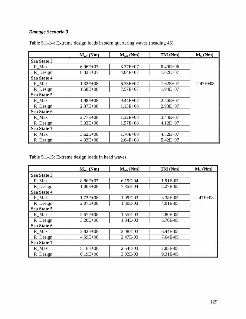
Damage Scenario 3 Table 5.1-14: Extreme design loads in stern quartering waves (heading 45) Mwv (Nm) Mwh (Nm) TM (Nm) MS (Nm) Sea State 3
R_Max 6.96E+07 3.37E+07 8.49E+06 R_Design 8.33E+07 4.04E+07 1.02E+07
Sea State 4 R_Max 1.32E+08 6.33E+07 1.62E+07 -2.47E+08 R_Design 1.58E+08 7.57E+07 1.94E+07
Sea State 5 R_Max 1.98E+08 9.44E+07 2.44E+07 R_Design 2.37E+08 1.13E+08 2.93E+07
Sea State 6 R_Max 2.77E+08 1.32E+08 3.44E+07 R_Design 3.32E+08 1.57E+08 4.12E+07
Sea State 7 R_Max 3.62E+08 1.70E+08 4.52E+07 R_Design 4.33E+08 2.04E+08 5.42E+07
Table 5.1-15: Extreme design loads in head waves Mwv (Nm) Mwh (Nm) TM (Nm) MS (Nm) Sea State 3
R_Max 8.86E+07 6.19E-04 1.91E-05 R_Design 1.06E+08 7.35E-04 2.27E-05
Sea State 4 R_Max 1.73E+08 1.09E-03 3.38E-05 -2.47E+08 R_Design 2.07E+08 1.30E-03 4.01E-05
Sea State 5 R_Max 2.67E+08 1.55E-03 4.80E-05 R_Design 3.20E+08 1.84E-03 5.70E-05
Sea State 6 R_Max 3.82E+08 2.08E-03 6.44E-05 R_Design 4.59E+08 2.47E-03 7.64E-05
Sea State 7 R_Max 5.16E+08 2.54E-03 7.85E-05 R_Design 6.19E+08 3.02E-03 9.31E-05
129

Table 5.1-16: Extreme design loads in beam waves Mwv (Nm) Mwh (Nm) TM (Nm) MS (Nm) Sea State 3
R_Max 1.09E+07 1.32E+07 9.41E+05 R_Design 1.30E+07 1.58E+07 1.12E+06
Sea State 4 R_Max 2.04E+07 2.50E+07 1.68E+06 -2.47E+08 R_Design 2.44E+07 2.98E+07 1.99E+06
Sea State 5 R_Max 3.07E+07 3.77E+07 2.41E+06 R_Design 3.67E+07 4.50E+07 2.86E+06
Sea State 6 R_Max 4.33E+07 5.32E+07 3.25E+06 R_Design 5.18E+07 6.36E+07 3.86E+06
Sea State 7 R_Max 5.75E+07 7.11E+07 4.00E+06 R_Design 6.88E+07 8.49E+07 4.75E+06
5.2 Prediction of extreme design loads using the results from the 2-D nonlinear method In this section short-term prediction is used to predict extreme design loads in irregular waves by using the results of the 2-D nonlinear method in regular waves. Strictly speaking the short-term prediction is only valid in the linear range, so it is not desirable to mix it with the 2-D nonlinear method. However this method can produce results quickly and fairly accurately. The 2-D nonlinear method has been used to calculate the wave-induced loads in the time domain in regular waves, and the time series has then been converted to RAOs for each load component. Finally the RAOs have been used in short-term predictions to calculate the extreme design value for each load component. An immediate issue to be addressed in this context is what wave amplitude should be used to calculate the RAOs because different wave amplitudes would lead to different values of RAOs due to the nonlinearity in the responses. Two wave amplitudes, namely 2.0 m and 2.5 m, have been chosen to calculate the RAOs of wave-induced loads in order to see how much difference there would be in the predicted extreme design loads. Firstly the 2-D nonlinear method has been applied to predict the extreme design value of the hogging and sagging bending moment at the cut of the ship model in the intact condition at head seas with duration of 96 hours under 2 different wave amplitudes, namely 2.0 m and 2.5 m. The results are presented in Table 5.2-1. Similarly the 2-D nonlinear method has been applied to predict the extreme design value of hogging and sagging bending moment at the cut of the ship model in damage scenario 2 at head seas with a duration of 12 hours under 2 different wave amplitudes. The results are shown in Table 5.2-2. It can be seen that the difference in extreme design loads (both hogging and sagging) between 2m and 2.5m wave heights is increasing with the increase of sea roughness, but always less than 6.62 percent in the intact condition and 6.60 percent in damage scenario 2. For hogging bending moments, the extreme design value based on
130

a 2-m wave height is greater than that based on a 2.5-m wave height, but it is the opposite case for the sagging bending moment. Table 5.2-1: Extreme design loads by the 2-D nonlinear method in the intact condition Mwv (N-m) , Hogging Mwv (N-m) , Sagging
(2m) (2.5m) Percent Difference
(2m) (2.5m) Percent Difference
Sea State 3 R_Max 7.83E+07 7.66E+07 2.22E+00 9.60E+07 1.01E+08 -4.95E+00R_Design 9.38E+07 9.18E+07 2.18E+00 1.15E+08 1.21E+08 -4.96E+00Sea State 4 R_Max 1.54E+08 1.51E+08 1.99E+00 1.88E+08 1.99E+08 -5.53E+00R_Design 1.85E+08 1.81E+08 2.21E+00 2.26E+08 2.39E+08 -5.44E+00Sea State 5 R_Max 2.39E+08 2.33E+08 2.58E+00 2.91E+08 3.09E+08 -5.83E+00R_Design 2.87E+08 2.80E+08 2.50E+00 3.49E+08 3.71E+08 -5.93E+00Sea State 6 R_Max 3.43E+08 3.34E+08 2.69E+00 4.18E+08 4.45E+08 -6.07E+00R_Design 4.12E+08 4.00E+08 3.00E+00 5.01E+08 5.34E+08 -6.18E+00Sea State 7 R_Max 4.60E+08 4.46E+08 3.14E+00 5.64E+08 6.04E+08 -6.62E+00R_Design 5.52E+08 5.35E+08 3.18E+00 6.77E+08 7.25E+08 -6.62E+00
131

Table 5.2-2: Extreme design loads by the 2-D nonlinear method in DS 2 Mwv (Nm) Hogging Mwv (Nm) Sagging
(2m) (2.5m) Percent Difference
(2m) (2.5m) Percent Difference
Sea State 3
R_Max 6.31E+07 6.17E+07 2.27E+00 7.74E+07 8.13E+07 -4.80E+00R_Design 7.84E+07 7.67E+07 2.22E+00 9.62E+07 1.01E+08 -4.75E+00Sea State 4 R_Max 1.24E+08 1.21E+08 2.48E+00 1.52E+08 1.61E+08 -5.59E+00R_Design 1.55E+08 1.51E+08 2.65E+00 1.89E+08 2.00E+08 -5.50E+00Sea State 5 R_Max 1.93E+08 1.88E+08 2.66E+00 2.35E+08 2.49E+08 -5.62E+00R_Design 2.40E+08 2.34E+08 2.56E+00 2.92E+08 3.10E+08 -5.81E+00Sea State 6 R_Max 2.77E+08 2.69E+08 2.97E+00 3.37E+08 3.59E+08 -6.13E+00R_Design 3.44E+08 3.34E+08 2.99E+00 4.19E+08 4.47E+08 -6.26E+00Sea State 7 R_Max 3.71E+08 3.59E+08 3.34E+00 4.55E+08 4.87E+08 -6.57E+00R_Design 4.61E+08 4.47E+08 3.13E+00 5.66E+08 6.06E+08 -6.60E+00
In order to further evaluate the results from the 2-D nonlinear method, RAOs obtained in the experimental tests have been used to predict extreme design loads. Similarly two different sets of wave amplitudes, namely large amplitude waves and very large amplitude waves, have been used separately to calculate the extreme design loads. Because the experimental data were available only at the cut (the section where the force gauge was installed) of the ship model, the extreme design loads presented in this section were for the ship model at the cut, which was 54.5 cm apart from the AP. The Sea Area 16 of the Atlantic Ocean under Sea State 3 to Sea State 7 was used in short term predictions. A duration of 96 hours was used in the short-term prediction for the intact condition while a reduced duration of 12 hours, which was recommended in Lloyds Register’s Navy Vessel Rule (Lloyds Register of Shipping, 2002), was used for damage scenario 2. The results of the above calculations have been presented in Tables 5.2-3 and 5.2-4 for the intact condition and damage scenario 2 respectively.
132

In addition, also presented in Tables 5.2-3 and 5.2-4 are the results obtained from the analytical formulae, which were recommended in Lloyds Register’s Navy Vessel Rules (Lloyds Register of Shipping, 2002). The details of the formulae used in this study are presented in Appendix D. Table 5.2-3: Extreme vertical bending moment in the intact condition Extreme Design
Load (Nm), Hogging Extreme Design Load (Nm), Sagging
Sagging/Hogging Ratio
Nonlinear methoda 5.52E+08 6.77E+08 1.23 Nonlinear methodb 5.35E+08 7.25E+08 1.36
Rulesc 5.58E+08 7.00E+08 1.25 Experimentd 4.01E+08 5.45E+08 1.36 Experimente 3.67E+08 5.22E+08 1.42
Linear method 5.52E+08 5.52E+08 1.00 Table 5.2-4: Extreme vertical bending moment in damage scenario 2 Extreme Design
Load (Nm), Hogging Extreme Design Load (Nm), Sagging
Sagging/Hogging Ratio
Nonlinear methoda 4.61E+08 5.66E+08 1.23 Nonlinear methodb 4.47E+08 6.06E+08 1.36 Rulesc 3.13E+08 3.92E+08 1.25 Experimentd 3.35E+08 4.55E+08 1.36 Experimente 3.07E+08 4.36E+08 1.42 Linear method 5.38E+08 5.38E+08 1.00
The footnotes for Tables 5.2-3 and 5.2-4 are as follows: a: Using RAOs from the 2-D nonlinear method under constant wave amplitude 2m. b: Using RAOs from the 2-D nonlinear method under constant wave amplitude 2.5m. c: Using the formulae in Lloyds Register’s Navy Vessel Rules. d: Using RAOs obtained from the experiment with large wave amplitude. e: Using RAOs obtained from the experiment with very large wave amplitude.
From Table 5.2-3 it can be seen that the 2-D nonlinear method overestimates the extreme design hogging bending moment by 37.7 percent and 45.8 percent for 2.0m and 2.5m wave heights respectively. Similarly it overestimates the extreme design sagging bending moment by 24.2 percent and 38.9 percent. However the 2-D linear method overestimates the extreme design hogging bending moment by 37.7 percent and 50.4 percent for 2.0m and 2.5m wave heights respectively, and overestimates the extreme design sagging bending moment by 1.3 percent and 5.8 percent for 2.0m and 2.5m wave heights respectively. Hence the results in the intact condition are slightly in favour of the 2-D linear method.
133

Similar comparison has also been applied to the results in Table 5.2-4. The 2-D nonlinear method overestimates the extreme design hogging bending moment by 37.6 percent and 45.6 percent for 2.0m and 2.5m wave heights respectively, and overestimates the extreme design sagging bending moment by 24.4 percent and 39.0 percent. However the 2-D linear method overestimates the extreme design hogging bending moment by 60.6 percent and 75.2 percent for 2.0m and 2.5m wave heights respectively, and overestimates extreme design sagging bending moment by 18.2 percent and 23.4 percent for 2.0m and 2.5m wave heights respectively. Therefore the accuracy of the 2-D linear method is almost as good as that of the 2-D nonlinear method in damage scenario 2. In Table 5.2-3, both hogging and sagging bending moments for the 2-D nonlinear method agree well with those of the LR Rules’ formulae. However the hogging bending moment of the 2-D linear method agrees well with that of the LR Rules’ formulae, but agreement in the sagging bending moment is not as good as with the hogging bending moment because in the 2-D linear method the sagging bending moment is the same as hogging bending moment. It should be pointed out that the extreme design value predicted by LR Rules is the maximum value for the ship model. In another words, the extreme design value at the cut is the same as that of the sections at amidships because the cut is not far away from amidships. However the extreme design value predicted by the 2-D nonlinear method at the cut could potentially be quite different from that of the sections at amidships, where the maximum vertical bending moment would occur. This might at least partly explain why LR Rules produces the largest extreme design hogging and sagging moments in the intact condition. The ratio of sagging bending moment to hogging bending moment of the 2-D nonlinear method is in good agreement with that of the experimental tests. This is an advantage of the 2-D nonlinear method over the 2-D linear method. 5.3 Load combinations for strength assessment The load components are combined for both the intact condition and damage scenario 1 using the methods described in section 3.2, based on the results predicted by the 2-D linear method. The loads are for the cross-section, which is 70.5 meters from the AP. The details are presented in Tables 5.3-1 and 5.3-2.
134

Table 5.3-1 Load combinations in intact condition at 45 degree heading
Basic Loads Ms = 1.65E+08
RAOmaxMy = 7.68E+07 RAOmax
Mz = 4.25E+07 RAOmaxMx = 1.74E+07
1ω = 0.85 2ω = 0.75 3ω = 0.75 RAO2
My = 6.92E+07 RAO1Mz= 3.48E+07 RAO1
Mx = 3.76E+06 RAO3
My = 6.92E+07 RAO3Mz = 4.25E+07 RAO2
Mx = 1.74E+07 Load Combinations
Sea State 3 MY
max = 8.63E+07 MZ max = 4.32E+07 MX
max = 1.22E+07 Heq 1 = 1.12E+00 Heq 2 = 1.02E+00 Heq 3 = 7.01E-01
Load combination without Ms My component Mz component Mx component LC1 8.63E+07 3.91E+07 4.23E+06 LC2 7.03E+07 4.32E+07 1.77E+07 LC3 4.85E+07 2.98E+07 1.22E+07 Sea State 4
MY max = 1.63E+08 MZ
max = 8.12E+07 MX max = 2.29E+07
Heq 1 = 2.12E+00 Heq 2 = 1.91E+00 Heq 3 = 1.32E+00 Load combination without Ms My component Mz component Mx component LC1 1.63E+08 7.39E+07 7.98E+06 LC2 1.32E+08 8.12E+07 3.32E+07 LC3 9.11E+07 5.59E+07 2.29E+07 Sea State 5
MY max = 2.45E+08 MZ
max = 1.21E+08 MX max = 3.42E+07
Heq 1 = 3.19E+00 Heq 2 = 2.85E+00 Heq 3 = 1.97E+00 Load combination without Ms My component Mz component Mx component LC1 2.45E+08 1.11E+08 1.20E+07 LC2 1.97E+08 1.21E+08 4.95E+07 LC3 1.36E+08 8.35E+07 3.42E+07 Sea State 6
MY max = 3.44E+08 MZ
max = 1.69E+08 MX max = 4.75E+07
Heq 1 = 4.48E+00 Heq 2 = 3.98E+00 Heq 3 = 2.73E+00 Load combination without Ms My component Mz component Mx component LC1 3.44E+08 1.56E+08 1.68E+07 LC2 2.75E+08 1.69E+08 6.92E+07 LC3 1.89E+08 1.16E+08 4.75E+07
135

Table 5.3-1 Load combinations in intact condition at 45 degree heading Sea State 7
MY max = 4.49E+08 MZ
max = 2.18E+08 MX max = 6.09E+07
Heq 1 = 5.85E+00 Heq 2 = 5.13E+00 Heq 3 = 3.50E+00 Load combination without Ms My component Mz component Mx component LC1 4.49E+08 2.03E+08 2.20E+07 LC2 3.55E+08 2.18E+08 8.93E+07 LC3 2.42E+08 1.49E+08 6.09E+07
Table 5.3-2 Load combinations in damage scenario 1 at 45 degree heading
Basic Loads Ms 5.51E+07
RAOmaxMy = 7.65E+07 RAOmax
Mz= 3.99E+07 RAOmaxMx = 1.27E+07
1ω = 0.85 2ω = 0.8 3ω = 0.8 RAO2
My = 7.65E+07 RAO1Mz = 3.59E+07 RAO1
Mx = 7.05E+06 RAO3
My = 7.65E+07 RAO3Mz = 3.99E+07 RAO2
Mx = 1.27E+07 Load Combinations
Sea State 3 MY
max = 8.95E+07 MZ max = 4.57E+07 MX
max = 9.74E+06 Heq 1 = 1.17E+00 Heq 2 = 1.15E+00 Heq 3 = 7.67E-01
Load combination without Ms My component Mz component Mx component LC1 8.95E+07 4.20E+07 8.25E+06 LC2 8.76E+07 4.57E+07 1.45E+07 LC3 5.87E+07 3.06E+07 9.74E+06 Sea State 4
MY max = 1.70E+08 MZ
max = 8.52E+07 MX max = 1.83E+07
Heq 1 = 2.22E+00 Heq 2 = 2.14E+00 Heq 3 = 1.44E+00 Load combination without Ms My component Mz component Mx component LC1 1.70E+08 7.98E+07 1.57E+07 LC2 1.63E+08 8.52E+07 2.71E+07 LC3 1.10E+08 5.75E+07 1.83E+07 Sea State 5
MY max = 2.57E+08 MZ
max = 1.27E+08 MX max = 2.72E+07
Heq 1 = 3.36E+00 Heq 2 = 3.18E+00 Heq 3 = 2.14E+00
136

Table 5.3-2 Load combinations in damage scenario 1 at 45 degree heading
Load combination without Ms My component Mz component Mx component LC1 2.57E+08 1.21E+08 2.37E+07 LC2 2.43E+08 1.27E+08 4.04E+07 LC3 1.64E+08 8.55E+07 2.72E+07 Sea State 6
MY max = 3.62E+08 MZ
max = 1.76E+08 MX max = 3.79E+07
Heq 1 = 4.73E+00 Heq 2 = 4.41E+00 Heq 3 = 2.98E+00 Load combination without Ms My component Mz component Mx component LC1 3.62E+08 1.70E+08 3.34E+07 LC2 3.37E+08 1.76E+08 5.60E+07 LC3 2.28E+08 1.19E+08 3.79E+07 Sea State 7
MY max = 4.75E+08 MZ
max = 2.25E+08 MX max = 4.87E+07
Heq 1 = 6.21E+00 Heq 2 = 5.64E+00 Heq 3 = 3.83E+00 Load combination without Ms My component Mz component Mx component LC1 5.30E+08 2.23E+08 4.38E+07 LC2 4.86E+08 2.25E+08 7.16E+07 LC3 3.48E+08 1.53E+08 4.87E+07
137
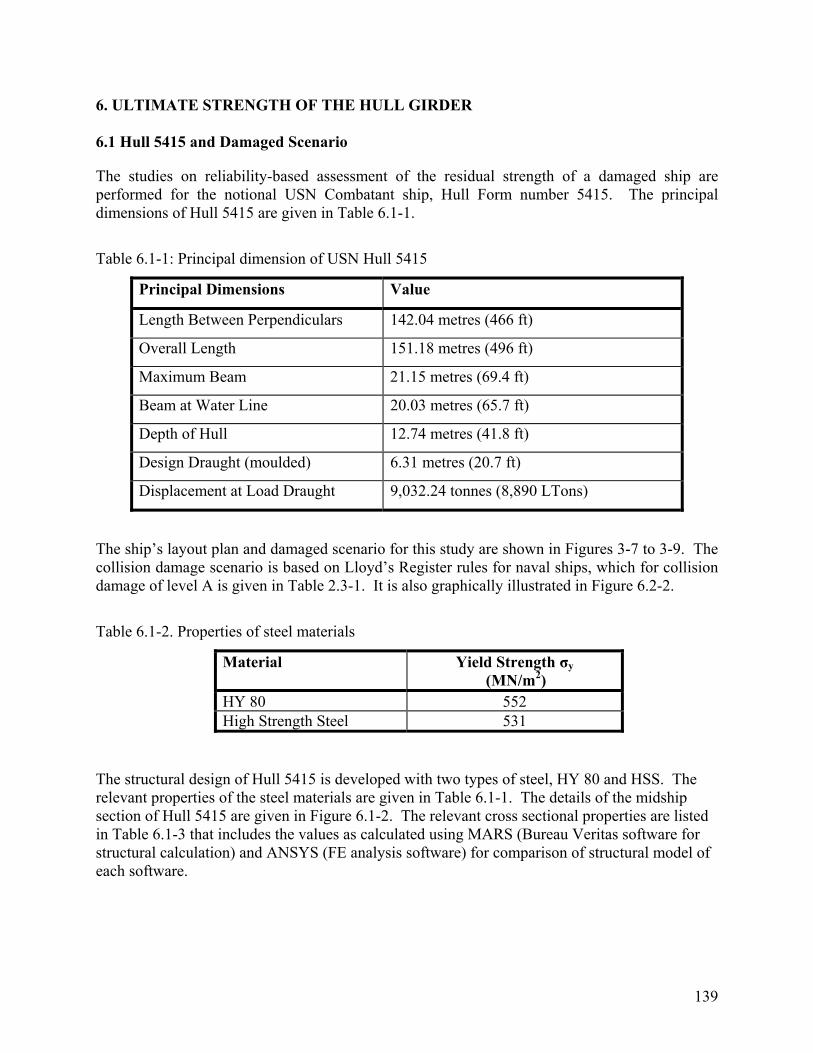
6. ULTIMATE STRENGTH OF THE HULL GIRDER 6.1 Hull 5415 and Damaged Scenario
The studies on reliability-based assessment of the residual strength of a damaged ship are performed for the notional USN Combatant ship, Hull Form number 5415. The principal dimensions of Hull 5415 are given in Table 6.1-1.
Table 6.1-1: Principal dimension of USN Hull 5415
Principal Dimensions Value
Length Between Perpendiculars 142.04 metres (466 ft)
Overall Length 151.18 metres (496 ft)
Maximum Beam 21.15 metres (69.4 ft)
Beam at Water Line 20.03 metres (65.7 ft)
Depth of Hull 12.74 metres (41.8 ft)
Design Draught (moulded) 6.31 metres (20.7 ft)
Displacement at Load Draught 9,032.24 tonnes (8,890 LTons)
The ship’s layout plan and damaged scenario for this study are shown in Figures 3-7 to 3-9. The collision damage scenario is based on Lloyd’s Register rules for naval ships, which for collision damage of level A is given in Table 2.3-1. It is also graphically illustrated in Figure 6.2-2.
Table 6.1-2. Properties of steel materials
Material Yield Strength σy (MN/m2)
HY 80 552 High Strength Steel 531
The structural design of Hull 5415 is developed with two types of steel, HY 80 and HSS. The relevant properties of the steel materials are given in Table 6.1-1. The details of the midship section of Hull 5415 are given in Figure 6.1-2. The relevant cross sectional properties are listed in Table 6.1-3 that includes the values as calculated using MARS (Bureau Veritas software for structural calculation) and ANSYS (FE analysis software) for comparison of structural model of each software.
139

Figure 6.1-1: Midship scantlings of Hull 5415
140

Table 6.1-3: Cross section characteristics
Parameter Value (MARS) Value (ANSYS)
Total Section Area 1.2592 m2 1.2576 m2
Neutral axis above baseline 6.57486 m 6.5119 m
Vertical Moment of Inertia 28.968810 m4 28.995 m4
Horizontal Moment of Inertia 43.141570 m4 43.11 m4
In accordance with BV rules for ships with Cb less then 0.8, the requirement for section modulus is: ZR, Min = n1 C L2 B (CB + 0.7) k 10-6 (6.1.1) The comparison of the required section modulus properties as per BV rules and the actual for Hull 5415 midship section is given in Table 6.1-4. Table 6.1-4: Section modulus required as per BV Rules and actual for the midship section.
Parameter BV Rule Hull 5415
Deck 3.2728 m3 4.6912 m3
Bottom 3.0655 m3 4.4060 m3
Vertical Moment of Inertia 21.1343 m4 28.968810 m4
6.2 Ultimate Hull Girder Strength – using MARS
The MARS software from Bureau Veritas is used to calculate ultimate hull girder strength using the beam-column idealization of the Smith Method. The MARS software provides different failure mode algorithms for calculation of ultimate strength that include the Elastic Ideally Plastic (EIP) failure mode and the Beam-Column (BC) failure mode, apart from the others.
As already discussed in Section 2.3, for the EIP failure mode material beyond the elastic limit is considered fully plastic under both tension and compression. The Beam-Column method of MARS uses the load-end shortening curves given in Equation 2.3-1.
The MARS calculations are performed for both the intact and damaged conditions. Figure 6.2-1 shows the intact ship section modelled for the MARS calculations. The damaged cross section shown in Figure 6.2-2 is modelled as per LR recommended damaged structure sizes as discussed Section 3.3. Figure 6.2-3 shows the MARS calculation results for ultimate strength in pure horizontal bending of Hull 5415 for the elastic ideally plastic failure mode. The results for ultimate strength in pure
141

vertical bending for the beam-column failure mode are given in Figure 6.2-4. The ultimate vertical moment capacity for the elastic-plastic failure mode is 2.556 GN-m whereas the ultimate moment capacity for the beam-column failure mode is 1.561 GN-m. The ultimate moment capacity for the beam-column mode is 38.92 percent lower than that for the elastic-plastic failure mode since the beam-column method is based on load shortening curves that take into count the shear lag, residual stress, and initial deformation along with other production related effects. The ultimate bending moment capacity for the combination of vertical and horizontal moments is given in Figures 6.2-5 and 6.2-6 for the elastic-plastic failure mode and in Figures 6.2-7 and 6.2-8 for the beam-column method. These results are for the intact ship in the hogging condition. The MV and MH interaction formulae in the form of equation 2.3-6 are as follows: −− For the elastic ideally plastic failure mode (Also see Figure 6.2-6).
104339.262467.1
=⎟⎟⎠
⎞⎜⎜⎝
⎛+⎟⎟
⎠
⎞⎜⎜⎝
⎛
HU
H
VU
V
MM
MM
(6.2.1)
−− For the beam-column failure mode (Also see Figure 8.2-8).
12.355114.53198
=⎟⎟⎠
⎞⎜⎜⎝
⎛+⎟⎟
⎠
⎞⎜⎜⎝
⎛
HU
H
VU
V
MM
MM
(6.2.2)
The comparison of ultimate moment capacity of the intact condition and damaged condition DS1 in terms of a vertical and horizontal moment interaction diagram is given in Figure 6.2-9 for both hogging and sagging conditions. For the damaged ship, the vertical and horizontal moment interaction formula derived from interaction terms as plotted in Figure 6.2-9 are as follows: −− For the damaged ship hogging condition
13.457752.7489
=⎟⎟⎠
⎞⎜⎜⎝
⎛+⎟⎟
⎠
⎞⎜⎜⎝
⎛
HU
H
VU
V
MM
MM
(6.2.3)
−− For the damaged ship sagging condition
11.821551.9713
=⎟⎟⎠
⎞⎜⎜⎝
⎛+⎟⎟
⎠
⎞⎜⎜⎝
⎛
HU
H
VU
V
MM
MM
(6.2.4)
The comparison of the ultimate moment for various bending curvature ratios (the ratio of horizontal to vertical bending) in the hogging condition for the intact and damaged ship is shown in Figure 6.2-10. It may be observed that for the hogging condition when the bending curvature ratio is small and consequently, predominant curvature is in the vertical direction depicting the predominant vertical bending moment, the difference between the ultimate moment for damaged and intact conditions is small. As the curvature ratio increases, the horizontal moment also increases and the difference between the intact and damaged conditions ultimate moments slowly increases until the curvature ratio reaches a value of about 2 and almost remains steady for further increases in curvature ratio, where the dominant moment is horizontal in nature. The
142

ultimate moment capacity of the damaged ship in the hogging condition is higher than that in the case of the intact ship for same loading condition, which is about 1 percent higher for pure vertical bending curvature and increases to about 11 percent for pure horizontal bending curvature as shown in Figure 6.2-12. The increase of ultimate moment capacity of the damaged ship in the hogging condition is attributed to a shift and change of the orientation of the neutral axis as shown in Figures 6.2-16 and 6.2-17. For the sagging condition, the ultimate moment capacity of the damaged ship decreases with an increase in the horizontal/vertical curvature ratio as shown in Figure 6.2-11. For the sagging ship condition, the curvature ratio around zero represents a predominant vertical moment resulting in compression in the damaged section of the ship. For the dominant vertical moment, the ultimate moment capacity of the damaged ship is reduced by 20 percent compared to that of the intact ship as shown in Figure 6.2-11. For a dominant horizontal moment i.e. for higher curvature ratio, the difference between ultimate moment capacity of the intact and the damaged ship is reduced to around 10 percent. The ultimate moment capacity of the damaged ship as a function of damage depth for the ultimate vertical moment in the sagging condition, ultimate vertical moments in the hogging condition, and ultimate horizontal moments are shown in Figures 6.2-13, 6.2-14, and 6.2-15, respectively. The results presented in these graphs are obtained using the beam-column method for ultimate strength calculation. Such functional representation of damage vs. ultimate strength at various sections across whole length of ship may be an appropriate tool for residual strength assessment of a damaged ship and quick assessment of risk in case of a damage incident.
143

Figure 6.2-1: Midship section, MARS model intact ship
Figure 6.2-2: Midship section, MARS model damaged condition
5.5
4.2
NA NA Damaged 0.104 m
144

Figure 6.2-3: Elastic – Ideally Plastic ultimate strength of Hull 5415 in pure horizontal bending.
145

Figure 6.2-4: Beam-column failure mode ultimate strength of Hull 5415 in pure vertical bending
146

2300000
2350000
2400000
2450000
2500000
2550000
2600000
0 0.1 0.2 0.3 0.4 0.5 0.6 0.7 0.8 0.9 1M Ratio
Mu
(KN
m)
Elastic - Perfectly Plastic Failure Mode
Figure 6.2-5: EIP ultimate strength of Hull 5415 for vertical and horizontal moments
00.10.20.30.40.50.60.70.80.9
11.11.2
0 0.1 0.2 0.3 0.4 0.5 0.6 0.7 0.8 0.9 1
MARS calculation ¦
Fitted function ?
Elastic-Perfectly Plastic Failure
Figure 6.2-6: EIP ultimate strength for vertical and horizontal moments interaction
147

1,400,000
1,450,000
1,500,000
1,550,000
1,600,000
1,650,000
1,700,000
1,750,000
1,800,000
0 0.1 0.2 0.3 0.4 0.5 0.6 0.7 0.8 0.9 1
M Ratio
Mu
(KN
m)
Beam – Column Failure Mode
Figure 6.2-7: BC ultimate strength of Hull 5415 for vertical and horizontal moments
0
0.1
0.2
0.3
0.4
0.5
0.6
0.7
0.8
0.9
1
1.1
0 0.1 0.2 0.3 0.4 0.5 0.6 0.7 0.8 0.9 1 1.1 1.2
Beam – Column Failure Mode
MARS calculation
Fitted function
Figure 6.2-8: BC ultimate strength of Hull 5415 for vertical and horizontal interaction
148

Figure 6.2-9: Comparison of Mv/Muv and Mh/Muh for intact and damaged conditions
Figure 6.2-10: Ultimate hogging moment for intact and damaged conditions
149

Figure 6.2-11: Comparison of ultimate moment for intact and damaged sagging conditions
Figure 6.2-12: Percentage reduction in ultimate hogging and sagging moment for intact and
damaged conditions
150

Figure 6.2-13: Ultimate sagging moment as function of damaged depth
Figure 6.2-14: Ultimate hogging moment as a function of damaged depth
151
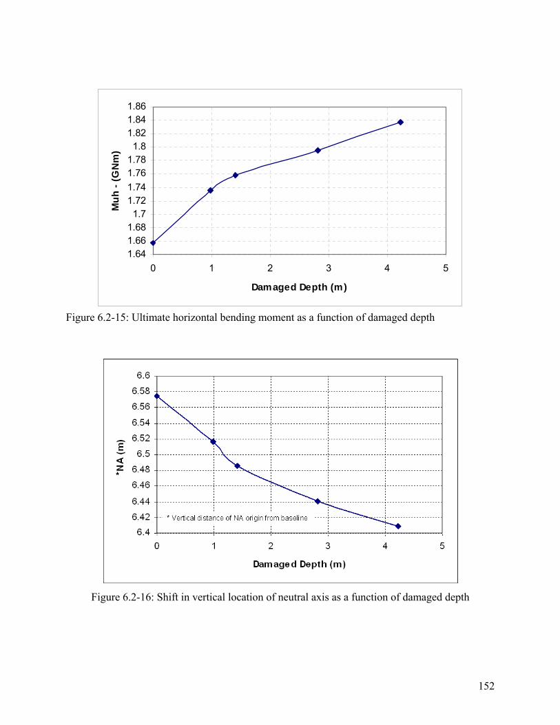
1.641.661.681.7
1.721.741.761.781.8
1.821.841.86
0 1 2 3 4 5
Damaged Depth (m)
Muh
- (G
Nm
)
Figure 6.2-15: Ultimate horizontal bending moment as a function of damaged depth
Figure 6.2-16: Shift in vertical location of neutral axis as a function of damaged depth
152

Figure 6.2-17: Inclination angle of neutral axis as a function of damaged depth 6.3 Ultimate Hull Girder Strength – using ANSYS ANSYS was used for FE analysis of Hull 5415 to determine the ultimate strength of the hull girder. In FE analysis, the size of ship structure to be used in FE model is required to be carefully determined. Some suggestions were made in the project kick-off meeting (21 Aug 2006) to develop a model of a complete ship using a top-down procedure starting from a coarse model to fine mesh. Considering the enormous amount of computing time in nonlinear analysis, this procedure was not considered realistic for the project because of budget constraints and enormous amount of computing time and effort that would be required. The large model will obviously give response of the structure for the entire hull length but is not necessarily required because in the 3-compartment model we are examining the critical sections of the hull girder. It was decided that a 3-compartment model would be sufficient as similar extent of structure is mostly recommended by classification societies for direct strength assessment of the primary supporting structure. The 3-compartment part of Hull 5415 is shown in Figure 6.3-1 is modelled for FE analysis.
153

Figure 6.3-1: The range of ship for FE modelling of damaged ship analysis However, structural details of the Hull 5415 were only available for the midship section and therefore the three compartments are considered to be the same in cross section as the midship section in these studies. Furthermore, no FE-based design assessment of the intact ship was available to compare the results with that of the damaged ship. The FE analysis for ultimate strength of hull girder was therefore carried out for both intact and damaged conditions.
6.3.1 Finite Element Model for nonlinear ultimate strength assessment
The 3-compartment models is large in term of FE computational time and since reliability-based assessment of the residual strength of the damaged ship using FE analysis requires a number of runs to generate the response surface, and because of budget constraints and time available for project completion, a 3-level FE modelling approach was adopted for this project, with a plan to compare the results from the large model with that of small model to assess the influence of boundary conditions. The reduced/small model was used for a large number of calculations for response surface development and reliability analysis. The reduced/small model analysis was however only possible for the intact ship. The three levels of FE models of ship in the intact condition are shown in Figure 6.3.1-1, which are the following:
• 3-compartment model • One compartment model • Two frame model
A full 3-compartment model was used for FE analysis of the ship in damaged conditions (see Figure 6.3.1-2). All the three models developed were for both the port and starboard side of the ship, i.e. no recourse was made to symmetry of structure about centreline, as apart from vertical and horizontal moments, torsion is also considered to be a dominant load for a damaged ship.
154

The ANSYS SHELL181 element was used in this analysis. SHELL181 is suitable for analysing thin to moderately thick shell structures. It is a 4-node element with six degrees of freedom at each node: translations in the x, y, and z directions, and rotations about the x, y, and z-axes. SHELL181 is well suited for linear, large rotation, and/or large strain nonlinear applications. Change in shell thickness is accounted for in nonlinear analyses. In the element domain, both full and reduced integration schemes are supported. SHELL181 counts for follower (load stiffness) effects of distributed pressures. The 3-compartment FE model of the ship structure is discretised in two major meshing sizes. The middle part of the middle compartment up to one frame inside of the bulkheads is fine meshed with average element size of 8 to 10 cm. For remaining part of the model a comparative coarse mesh of 35 to 40 cm was used in order to reduce the number of nodes and elements of the FE model. The 3-compartment model in total consists of around 0.4 million nodes and 0.41 million elements. The fine mesh in the middle compartment was required to suitably simulate structural damage using ANSYS/LS DYNA explicit FE analysis. The 1-compartment model mainly consists of a coarse mesh of average size between 50 and 70 cm. The FE model consists of about 45 thousand nodes and 42 thousand elements. A fine FE mesh was used for the 2-frame model, which consists of 52 thousand nodes and 51 thousand elements. The ship’s structural model for damaged case analysis was generated using explicit dynamic FE simulation of collision between two ships. A typical bow structure for a merchant vessel was modelled for collision impact approximately in the centre of the middle compartment at right angles to the longitudinal-central vertical plane of hull 5415. The damaged part of hull 5415 as obtained subsequent to collision simulation is shown in Figure 6.3.1-2. Figure 6.3.1-3 shows residual stress distributions in the deformed structure. The overly deformed elements from the damaged part of the model were removed in order to avoid computational divergence in subsequent static nonlinear FE analysis that was used to determine the ultimate moment capacity of the damaged hull. The refined element mesh of the damaged structural model is shown in Figure 6.3.1-4 along with residual stress vectors.
155

Figure 6.3.1-1: Different odels for FE Analysis.
Figure 6.3.1-2: Damaged structural model ANSYS/LS DYNA simulation.
m
5.5
4.5
5.5
Cut Away – View Damaged section
Three Compartment Model
Coarse Mesh Size 35- 40 cm
Fine Mesh Size 8-10 cm
Nodes: 0.4 million .41 million Elements: 0
One Compartment Mo
way – View from Ce
del
Fine Mesh Size 8-10 cm
ousands thousands
ame Model
Cut AHalf ntre
Mesh Size 50- 70 cm
Nodes: 45 thousands thousandsElements: 42
Nodes: 52 thElements: 51
Two Fr
156
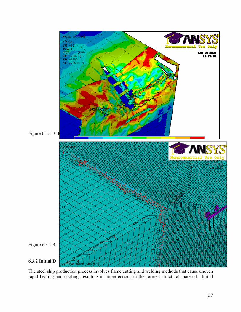
Figure 6.3.1-3: Residual stress in the damaged part of model structure
Figure 6.3.1-4: Refined mesh of damaged structure
6.3.2 Initial Deformations
The steel ship production process involves flame cutting and welding methods that cause uneven rapid heating and cooling, resulting in imperfections in the formed structural material. Initial
157

deformation arising out of the production process may considerably reduce the load bearing capacity of ship structure. There are a number of efforts made to model the initial deformation of welded structure based on analytical methods, numerical methods, and experimental/practical measurements e.g. Faulkner (1975), Carlsen and Czujko (1978), Antoniou (1980), Smith et al. (1988) and Masaoka (1996). Furthermore, classification societies also specify limitations on maximum initial deflection of plate on completion of fabrication. The post-weld initial deflections are represented by the following formula:
∑∑= =
=M
i
N
jijpl b
yjaxiBww
0 0000 sinsin ππ
(6.3.2.1)
Where a is plate length, b is plate breath. Boij indicates the welding induced initial deformation normalized by the maximum initial deflection, w0pl. The i and j are half wave numbers in the x and y directions. The values of maximum initial deflections proposed by different sources are given in Figure 6.3.2-1. Statistical analysis of proposed values relevant to structural plates of hull 5415 resulted in an average value of 0.00461m with a coefficient of variance of 0.508, which approximately follows a normal distribution as is apparent from the histogram in the figure. Figure 6.3.2-2 also shows the deflection wave pattern that is applied as initial deformation to the FE model with random maximum amplitude and a normal distribution as described above. The initial deformation is applied only to the middle part of the 3-compartment model. In the case of the 1-compartment and 2-frame model, the initial deformation is applied to the whole structure.
158

0 . 0 0 0 0 0
0 . 0 0 0 5 0
0 . 0 0 1 0 0
0 . 0 0 1 5 0
0 . 0 0 2 0 0
0 . 0 0 2 5 0
0 . 0 0 3 0 0
0 . 0 0 3 5 0
0 . 0 0 4 0 0
0 . 0 0 0 . 1 0 0 . 2 0 0 . 3 0 0 . 4 0 0 . 5 0 0 . 6 0 0 . 7 0
x ( m )
Initia
l Def
lect
ion
(m)
Figure 6.3.2-1: Initial deformation model for FE analysis
Figure 6.3.2-2: Initial deformation as applied to mid part of 3-compartment model.
6.3.3 Material Model
The ship’s hull structure is designed for two types of steels. The properties of steels are listed in Table 6.3.3-1 below. Both types of steel material are modelled as elastic-perfectly-plastic. Production related variations in strength of material such as residual stress due to welding, cold working etc are not considered directly as a random parameter in the FE analysis but were
159

counted for in the reliability analysis using uncertainty factors. Therefore, the yield strength and modulus of elasticity were taken as deterministic values in the FE analysis. Table 6.3.3-1: Statistics of yield strength, σy, of steel materials (MN/m2)
Material Mean COV Distribution Correlation
HY 80 552 0.08 Lognormal Independent
HSS 351 0.08 Lognormal Independent
6.3.4 Load modelling and boundary conditions
As already discussed in Section 3.2, in the present study only vertical bending moment, horizontal bending moment and torsion are considered and the effects of local loads on plate panels and on stiffener bending are ignored. The FE analysis was carried out to determine the ultimate strength for the following conditions:
• Vertical bending moment to determine ultimate vertical bending moment capacity oment to determine ultimate horizontal bending moment
6.3.4-1.
• Horizontal bending mcapacity.
• Torsion to determine ultimate capacity of the section in torsion • Combined load to determine response function for hull structure in the form similar
to equation 3.3-6 and also for interaction of three moments mentioned above. The incremental moment equivalent displacements were applied as loads on boundary nodes for nonlinear analysis and to achieve ultimate failure as shown in Figure
160
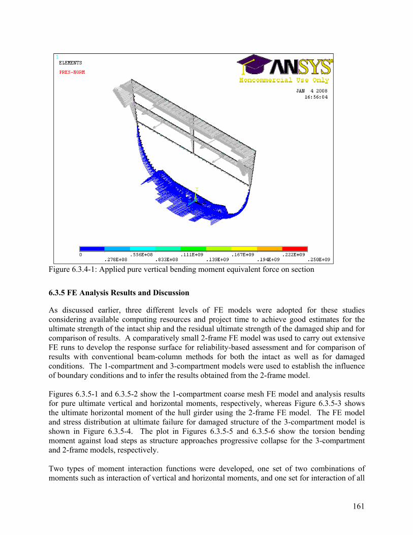
Figure 6.3.4-1: Applied pure vertical bending moment equivalent force on section
6.3.5 FE Analysis Results and Discussion
As discussed earlier, three different levels of FE models were adopted for these studies considering available computing resources and project time to achieve good estimates for the ultimate strength of the intact ship and the residual ultimate strength of the damaged ship and for comparison of results. A comparatively small 2-frame FE model was used to carry out extensive FE runs to develop the response surface for reliability-based assessment and for comparison of results with conventional beam-column methods for both the intact as well as for damaged
the influence f boundary conditions and to infer the results obtained from the 2-frame model.
partment coarse mesh FE model and analysis results
mbinations of oments such as interaction of vertical and horizontal moments, and one set for interaction of all
conditions. The 1-compartment and 3-compartment models were used to establisho Figures 6.3.5-1 and 6.3.5-2 show the 1-comfor pure ultimate vertical and horizontal moments, respectively, whereas Figure 6.3.5-3 shows the ultimate horizontal moment of the hull girder using the 2-frame FE model. The FE model and stress distribution at ultimate failure for damaged structure of the 3-compartment model is shown in Figure 6.3.5-4. The plot in Figures 6.3.5-5 and 6.3.5-6 show the torsion bending moment against load steps as structure approaches progressive collapse for the 3-compartment and 2-frame models, respectively. Two types of moment interaction functions were developed, one set of two com
161
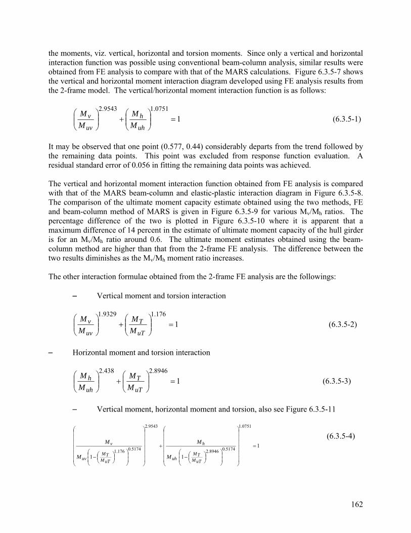
the moments, viz. vertical, horizontal and torsion moments. Since only a vertical and horizontal interaction function was possible using conventional beam-column analysis, similar results were obtained from FE analysis to compare with that of the MARS calculations. Figure 6.3.5-7 shows the vertical and horizontal moment interaction diagram developed using FE analysis results from the 2-frame model. The vertical/horizontal moment interaction function is as follows:
11.0752.9543⎞⎛⎞⎛ MM 1
=⎟⎜+⎟⎜ hv (6.3.5-1)
pared ith that of the MARS beam-column and elastic-plastic interaction diagram in Figure 6.3.5-8.
The comparison of the ultimate moment capacity estimate obtained using the two methods, FE and beam-column method of MARS is ve in Fi ure 6. 5-9 fopercentage difference of the two is plotted in Figure 6.3.5-10 where it is apparent that a
aximum difference of 14 percent in the estimate of ultimate moment capacity of the hull girder
⎟⎠
⎜⎝
⎟⎠
⎜⎝ uhuv MM
It may be observed that one point (0.577, 0.44) considerably departs from the trend followed by the remaining data points. This point was excluded from response function evaluation. A residual standard error of 0.056 in fitting the remaining data points was achieved. The vertical and horizontal moment interaction function obtained from FE analysis is comw
gi n g 3. r various Mv/Mh ratios. The
mis for an Mv/Mh ratio around 0.6. The ultimate moment estimates obtained using the beam-column method are higher than that from the 2-frame FE analysis. The difference between the two results diminishes as the Mv/Mh moment ratio increases. The other interaction formulae obtained from the 2-frame FE analysis are the followings:
− Vertical moment and torsion interaction
11.1761.9329
=⎟⎟⎠
⎞⎜⎜⎝
⎛+⎟⎟
⎠
⎞⎜⎜⎝
⎛
uT
T
uv
vMM
MM
(6.3.5-2)
− Horizontal moment and torsion interaction
12.89462.438⎞⎛⎞⎛ MM
=⎟⎜+⎟⎜ Th (6.3.5-3)
− Vertical moment, horizontal moment and torsion, also see Figure 6.3.5-11
⎟⎠
⎜⎝
⎟⎠
⎜⎝ uTuh MM
1
11
1.0751
5174.08946.2
2.9543
5174.0176.1=
⎟⎟⎟⎟⎟⎟
⎠
⎞
⎜⎜⎜⎜⎜⎜
⎝
⎛
⎟⎟⎠
⎞⎜⎜⎝
⎛⎟⎠⎞⎜
⎝⎛−
+
⎟⎟⎟⎟⎟⎟
⎠
⎞
⎜⎜⎜⎜⎜⎜
⎝
⎛
⎟⎟⎠
⎞⎜⎜⎝
⎛⎟⎠⎞⎜
⎝⎛−
uTMTM
uh
h
uTMTM
uv
v
M
M
M
M (6.3.5-4)
162

163
The comparison of ultimate moment capacity of the hull girder in the intact and damaged conditions is given in Table 6.3.5-1. Further, Table 6.3.5-2 gives the percentage of ultimate strength of the damaged hull in comparimoment capacity in torsion for the damaged hull is only 8 percent of the capacity of the ship in the intact c
son to ultimate strength of the intact ship. The ultimate
ondition.

Figure 6.3.5-1: Ultimate vertical moment capacity of the 1-compartment model
164

Section I d
Section Index
Load
Section Index Section Index
Section Index
Figure 6.3.5-2: Horizontal ultimate moment capacity of the 1-compartment model
165

Figure 6.3.5-3: Horizontal ultimate moment capacity of the 2-frame model
166

167
Figure 6.3.5-4: Deformation and stress distribution of damaged 3-compartment model

0
0.1
0.2
0.3
0.4
0.5
0.6
0.7
0.8
0.9
1
0 10 20 30 40 50 60 70 80 90 100
load step
Mt (
GNm
)
Three compartment
Figure 6.3.5-5: Ultimate torsion – 3-compartment FE analysis
-1.2
-1
-0.8
-0.6
-0.4
-0.2
0
0.2
6 11 16 21 26
Load step
Mt
( GN
m )
31
2 Frame model
Figure 6.3.5-6: Ultimate torsion – 2-frame FE model
168

00.10.20.30.40.50.60.70.80.9
11.11.2
0 0.1 0.2 0.3 0.4 0.5 0.6 0.7 0.8 0.9 1 1.1 1.2
2Fr FE
Fitted function
Figure 6.3.5-7: MV and Mh interaction – 2-frame FE analysis results
00.10.20.30.40.50.60.70.80.9
11.11.2
0 0.1 0.2 0.3 0.4 0.5 0.6 0.7 0.8 0.9 1 1.1 1.2
2Fr FE Data points
Beam-Column FailureElastic-Perfectly Plastic Failure
2Fr FE fitted function
Figure 6.3.5-8: Comparison of MARS results with 2-frame FE analysis results
169

0
0.5
1
1.5
2
2.5
0 2 4 6 8 10 12 14 16 18 20
(Mv/Mh)
Mu
(GN
m)
Beam-Column Method
FE 2Fr Response Surface
Figure 6.3.5-9: Comparison of ultimate moment, MARS and 2-frame FE results
0
2
4
6
8
10
12
14
16
0 2 4 6 8 10 12 14 16 18 20
(Mv/Mh)
%ag
e D
iff B
C-F
E
Figure 6.3.5-10: Ultimate moment, percentage difference between MARS and FE results
170

Figure 6.3.5-11: Interaction response surface for Mv, Mh and Mt moment; FE results
Table 6.3.5-1: Comparison of ultimate vertical bending moment from different methods (GN-m)
Method MARS ANSYS Item EIP BC FPMC CM 2-Frame
Model 3-Comp.
Intact 3-Comp. Damaged
MVU Hogging 2.3405 1.5609 2.1859 1.389 2.095 1.46 0.16 Sagging -2.3405 -1.3273 -2.1859 -1.0701 -1.1445 -1.28 -0.214
MHU 2.5587 1.657 2.5878 1.625 1.3199 1.079 +0.341
-0.281 MTU - - - 1.251 1.5611 0.898 0.0728 Key:
EIP BC FPMC CM 2FrM
Elastic- Ideally Plastic Failure Mode Beam Column Failure Mode (Smith’s Method) Full Plastic Moment Capacity of the section Coarse Mesh Model 2-Frame Model – fine mesh
171

172
Table 6.3.5-2: Comparison of ultimate strength of intact and damaged ship
Ultimate Moment (GN-m) Intact Damaged Damaged % of Intact
Vertical (sagging) -1.28 -0.214 17
Horizontal -1.079 0.341 32
-0.281 26
Torsion 0.898 -0.0728 8

7. RELIABILITY BASED ASSESSMENT OF INTACT AND DAMAGED STRUCTURE
The reliability-based assessment of hull structure was made for both intact and damaged conditions. The reliability assessment for the intact condition was made for the worse case scenario, Sea State 7, and lesser sea states, including three load combinations as identified from the ship loading analysis. The reliability analysis was carried out using the moment interaction formula given in equation 6.3.5-4. Accordingly, the limit state function is defined as follows:
( )( ) ( )( ) R
MM
uh
h
MM
uv
vSthv
uT
T
uT
T M
M
M
MMMMg χχ ×−
⎟⎟⎟
⎠
⎞
⎜⎜⎜
⎝
⎛
−+
⎟⎟⎟
⎠
⎞
⎜⎜⎜
⎝
⎛
−= 1
11),,(
1.0751
5174.08946.2
2.9543
5174.0176.1 (7-1)
Where Sχ and Rχ are the modelling uncertainty parameters (Faulkner et al., 1988) defined as follows:
responsepredictedresponseactual
=χ (7-2)
It is usual to assume in reliability analysis of ship structures the normal distribution for uncertainty parameters, the 10 percent variance Teixeira (1997) in ultimate strength modelling and 15 percent variance (Mansour et al., 1994) in load modelling as suggested in the references above. The stillwater bending moment is considered normally distributed. The extreme value Type-II distribution is taken for vertical, horizontal and torsion moment loads. For ultimate moment capacity of the hull, Weibull distribution is assumed. Because of time constraints, a complete interaction diagram for vertical moment, horizontal moment and torsion for damaged cases using FE analysis was not possible. The comparison between the vertical/horizontal moment for the damaged and intact conditions calculated using the beam-column method with that calculated with the 2-frame FE analysis shown in Figure 6.3.5-9 gives a small difference in the moment ratio, around 11 percent. Therefore the limit state function in equation 7-1 was used for reliability analysis of the damaged condition. A scaling is built into the function because of the ultimate vertical, horizontal and torsion moment capacities of structure that were used in evaluation. This assumption is considered reasonable to derive reliability the index in absence of a more accurate moment interaction function for damaged conditions. The reliability analysis was carried out using CALREL software to apply the First Order Reliability Method (FORM) and Monte Carlo Simulation (MCS). The reliability index and relevant probabilities as calculated are given in Table 7.1 for both the intact and damaged cases. The reliability index for the intact condition is a minimum 3.771 for load combination 1 (LC 1) in Sea State 7, which is the worse operating scenario for the ship. The reliability index is plotted in Figure 7-1 for the damaged scenarios against various sea states. As it is given in Table 7-1, the FORM calculation did not converge for load combination LC 2 for Sea State 5, and for all
173
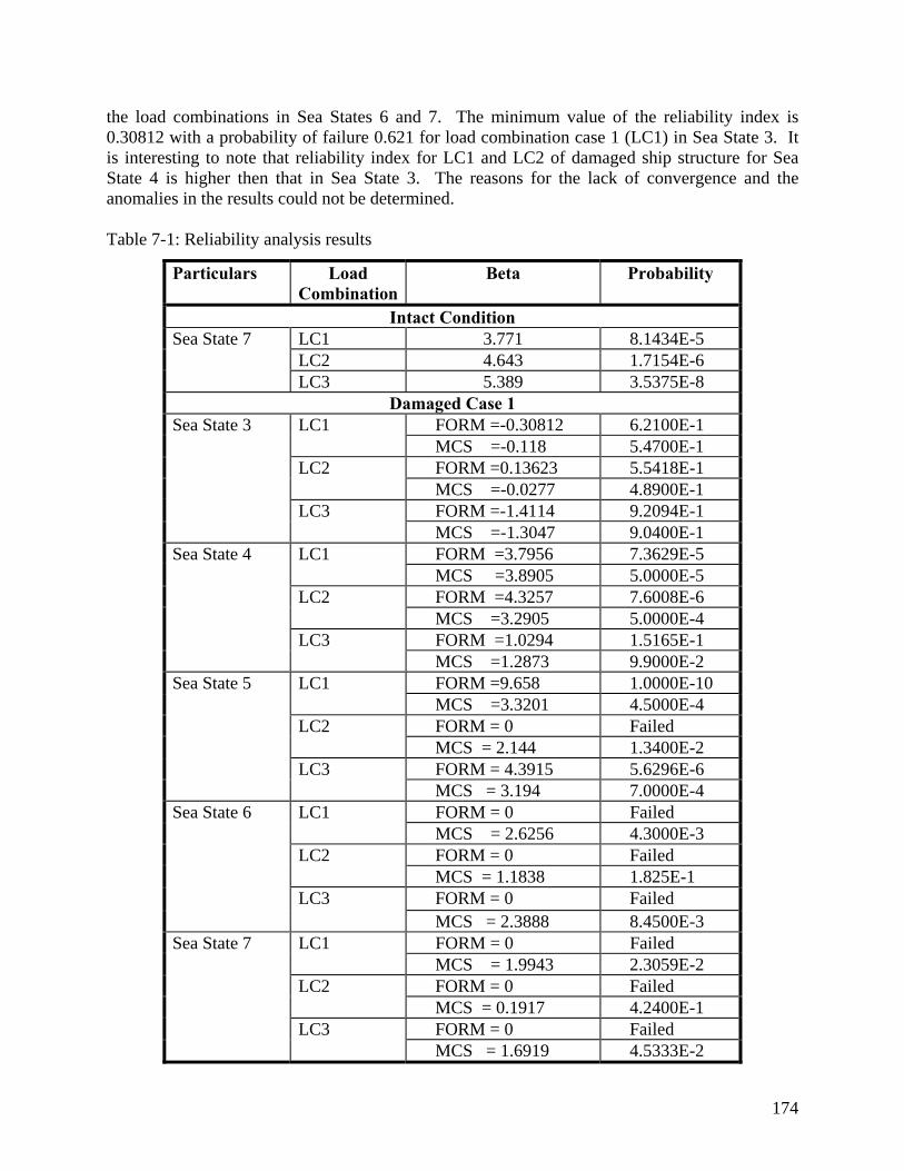
the load combinations in Sea States 6 and 7. The minimum value of the reliability index is 0.30812 with a probability of failure 0.621 for load combination case 1 (LC1) in Sea State 3. It is interesting to note that reliability index for LC1 and LC2 of damaged ship structure for Sea State 4 is higher then that in Sea State 3. The reasons for the lack of convergence and the anomalies in the results could not be determined. Table 7-1: Reliability analysis results
Particulars Load Combination
Βeta Probability
Intact Condition Sea State 7 LC1 3.771 8.1434E-5
LC2 4.643 1.7154E-6 LC3 5.389 3.5375E-8
Damaged Case 1 Sea State 3 LC1 FORM =-0.30812 6.2100E-1
MCS =-0.118 5.4700E-1 LC2 FORM =0.13623 5.5418E-1
MCS =-0.0277 4.8900E-1 LC3 FORM =-1.4114 9.2094E-1
MCS =-1.3047 9.0400E-1 Sea State 4 LC1 FORM =3.7956 7.3629E-5
MCS =3.8905 5.0000E-5 LC2 FORM =4.3257 7.6008E-6
MCS =3.2905 5.0000E-4 LC3 FORM =1.0294 1.5165E-1
MCS =1.2873 9.9000E-2 Sea State 5 LC1 FORM =9.658 1.0000E-10
MCS =3.3201 4.5000E-4 LC2 FORM = 0 Failed
MCS = 2.144 1.3400E-2 LC3 FORM = 4.3915 5.6296E-6
MCS = 3.194 7.0000E-4 Sea State 6 LC1 FORM = 0 Failed
MCS = 2.6256 4.3000E-3 LC2 FORM = 0 Failed
MCS = 1.1838 1.825E-1 LC3 FORM = 0 Failed
MCS = 2.3888 8.4500E-3 Sea State 7 LC1 FORM = 0 Failed
MCS = 1.9943 2.3059E-2 LC2 FORM = 0 Failed
MCS = 0.1917 4.2400E-1 LC3 FORM = 0 Failed
MCS = 1.6919 4.5333E-2
174
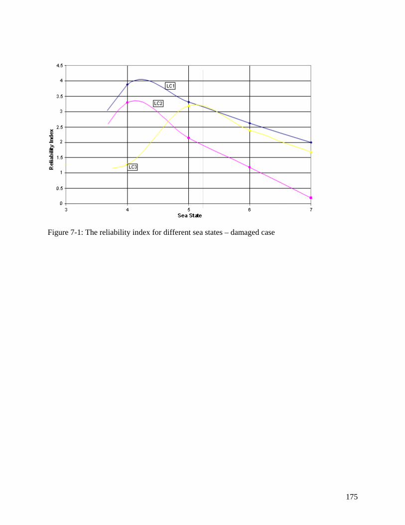
Figure 7-1: The reliability index for different sea states – damaged case
175

177
8. SUMMARY When a ship is damaged, the operators need to decide the immediate repair actions by evaluating the effects of the damage on the safety of the ship using a reliability-based residual strength assessment procedure. Assessment of the reliability of the damaged ship in various sea states will provide information on which such an evaluation can be made. There are significant differences between the conditions of an intact and a damaged ship that affect the procedures to be used in a reliability analysis.
• Damaged ships generally have heel and trim that are not part of the analysis of an intact ship.
• A damaged ship may have flooding that will significantly increase the displacement and therefore increase hydrodynamic loads in a seaway.
• The flooding of a damaged ship through an opening in the hull will be subject to inflow and outflow, which complicate the hydrodynamic loads estimation.
• The damage to the hull may have jagged edges and unusual residual stress patterns that will affect the ultimate strength of the hull girder.
• Openings in the hull may make considerations of loading by horizontal bending and torsion moments more important than for the intact ship.
• The damaged ship will be expected to operate for only a short time prior to repairs, so the sea spectra that will be encountered will be different from the lifetime loading spectra used in ship design.
This project has developed a procedure and tools for operators and decision makers to assess the loading, residual ultimate hull girder strength, and reliability of damaged ships for a given damage scenario. This study is a continuation of the NICOP project (Lee, et al 2006), in which an assessment procedure was developed. This procedure consists of four steps:
(1) Identify the location and size of the openings. Once a ship is damaged, the location and size in terms of length, height and depth of the penetration of the opening should be determined, so the degree of water ingress can be predicted.
(2) Calculate the still water bending moment and wave-induced loadings including vertical bending moment, horizontal bending moment and torsion. The floating conditions of the ship need to be calculated. The stillwater bending moment and wave-induced loads are then estimated. Because it is desirable to install the developed tools on board of ships for a quick and reliable assessment, computational time is a very important factor in choosing a particular method for both loading calculations and strength assessment.
(3) Calculate the ultimate hull girder strength of the damaged cross-section considering the interaction of vertical bending moment, horizontal bending moment and torsion. The ultimate hull girder strength of the damaged cross-section needs to be assessed. The interaction of vertical bending moment, horizontal bending moment and torsion should be considered. In addition, the strength of other cross-sections (not the damaged one), where the total load including stillwater bending moment and wave-induced loads under the damage conditions exceed that in intact condition, should also be assessed.

178
(4) Assess the structural integrity by deterministic and probabilistic approaches. The reliability of the damaged ship is calculated so a well-informed decision may be made based on this information.
In the current project, some tools for predicting wave-induced loads and assessing ultimate hull girder strength have been further developed and applied to a notional ship, US Navy Hull 5415. A fibreglass model with a scale of 1/100 was constructed with openings in the starboard side and with internal bulkheads and decks to limit the extent of flooding. The model had a transverse cut near midships with a force gauge installed to measure the vertical, horizontal, and torsion moments between the two sections of the hull. The model was tested in the Newcastle University towing tank, which is 37 metres long, 4 metres wide, and 1.2 metres deep, and equipped with a wave maker at one end and an energy absorbing beach at the other end. Tests were conducted at head, bow, beam, and quartering seas at three different regular wave heights and nine different wave frequencies. Testing was conducted with the ship in the intact condition and with two different damage scenarios, scenarios 2 and 3 from the previous study. For the damaged conditions, testing was conducted with flooding water free to flow into and out of the openings in the hull. The experimental results have revealed that the majority of the response RAOs show a nonlinear trend in which the non-dimensional responses are decreasing as wave amplitude increases in most frequency ranges, especially at the frequency where the responses achieve the maximum. For vertical bending moment this trend is very remarkable. It may be said that the high nonlinearity is an inherent feature of the sample vessel with a very fine hull form. Because the damage on the ship is unsymmetrical transversely with the openings on the starboard side, it is expected that the wave-induced loads might be different when the wave is approaching the ship model from different sides due to the dynamic behaviour of the flooded water in the damaged compartment. The test results have shown that the vertical bending moment at 45° wave heading at most of frequencies was slightly larger than that at 315° wave heading. There was no clear trend for horizontal bending moment at 45° and 315° wave headings. However, the horizontal bending moment in beam seas at 90° wave headings is slightly larger than that at 270° wave headings. The torsion moment at 315° wave headings is larger than that in 45° wave headings. A 2-D linear and a 2-D nonlinear method have been applied to the ship model to calculate the wave-induced loads in regular waves at the cut where the force gauge is installed in the model. The analyses simulated flooding with instantaneous changes in the height of floodwater to conform to the changes in wave height and pitch and roll of the hull. The Response Amplitude Operators (RAOs) computed from the numerical results have been compared with the RAOs computed from the experimental results. For the purpose of comparison, the experimental results were assumed as correct and differences in results attributed to the analyses. The 2-D linear method was shown to predict accurately wave-induced vertical bending moments in head seas and stern quartering seas, but the accuracy deteriorates with increases in wave amplitude. The accuracy in predicting the horizontal bending moment is not as good as that for

179
vertical bending moment, but is acceptable in most cases. However, the predictions of torsion moment are not satisfactory, although the magnitude of the torsion moments were low and did not affect the results of the study. Compared to the results from the experiments, the 2-D nonlinear method did not produce satisfactory results for vertical bending moment, horizontal bending moment and torsion moment in regular waves. Although this conclusion was largely based on the analysis of the results in 2-metre wave height, it was equally applicable to the results in 2.5-metre wave height. The predictions of torsion moment are the worst among the three components of the wave-induced loads, while the predictions of vertical bending moment have a similar level of accuracy to those of horizontal bending moment. The nonlinear method tends to produce better results at the resonant frequencies than at the other frequencies. However it should be pointed out that the measured wave heights were not equal to 2.0 metres, which was used in the numerical calculations, at most frequencies. Model uncertainties for both 2-D linear and nonlinear methods have been calculated. The model uncertainty factor, Xm, is defined as the ratio of the experimental load to the numerically predicted load. The accuracy of the estimated moments is measured by the mean and COV of the model uncertainty factor. For the 2-D linear method it is observed that the accuracy of the vertical bending moment is generally better than that of the horizontal bending moment and the torsion moment, and the accuracy for loads in head seas is much better than for those in stern quartering seas and beam seas. This could be mainly caused by the underwater hull form of the ship model with a small Cb compared with conventional ships. The COV of the horizontal bending moment is almost as twice as that of the vertical bending moment. The COV of the torsion moment is the largest of the three. Because of the large difference in COV for different force components it is more rational to consider the model uncertainties for vertical bending moment, horizontal bending moment and torsion moment separately in reliability analysis rather than using one combined model uncertainty for all the components. The 2-D linear method has a better mean and COV of Xm in the predictions of vertical bending moment and horizontal bending moment in both the intact condition and damage scenario 2 than the 2-D nonlinear method, and both 2-D linear and nonlinear methods have produced unsatisfactory results in torsion moment. Based on the current results, it may be said that the 2-D linear method is more accurate than the nonlinear method. However the nonlinear method can distinguish the difference between the positive and negative responses, but linear methods can’t. This advantage of the nonlinear method is especially important for ships with small block coefficient, such as frigates, etc. For a frigate the ratio of sagging bending moment to hogging bending moment could be as large as 1.78 (Clarke, 1986). In addition, hull girder strength in hogging is normally different from that in sagging. Therefore the nonlinear method is preferred. This slight preference of the nonlinear method was also based on another fact that the nonlinear method tends to produce better results in the resonant region than at other frequencies. Based on the current method for combining different load components, the accuracy in the resonant region is more important than that at other frequencies.

180
Extreme design loads in irregular waves based on the RAOs from the 2-D linear method, 2-D nonlinear method and experiment have been calculated for the ship model at the cut in the intact condition and damage scenario 2. The formulae recommended in the Lloyds Register’s rule for naval vessels (Lloyds Register of Shipping, 2002) have also been used to calculate the wave-induced extreme design loads. The results have demonstrated that the difference of extreme design loads (both hogging and sagging) between 2 m and 2.5 m wave height was increasing with the increase of sea roughness, but always less than 6.62 percent in the intact condition and 6.60 percent in damage scenario 2. For the hogging bending moment, the extreme design value based on the 2 m wave height is greater than that based on the 2.5m wave height, but it was opposite for sagging bending moment. Hence the effects of wave amplitude on the prediction of extreme design loads are modest. Both 2-D linear and nonlinear methods overestimate the extreme design loads compared with the experimental tests. The results are slightly in favour of the 2-D linear method in the intact condition, while the accuracy of the 2-D linear method is almost as good as that of the 2-D nonlinear method in damage scenario 2. Both hogging and sagging bending moments predicted by the 2-D nonlinear method agree well with those of LR Rules’ formulae. However the hogging bending moment of the 2-D linear method agrees well with that of LR Rules’ formulae, but agreement in sagging bending moment is not as good as in hogging bending moment because in the 2-D linear method the sagging bending moment is the same as the hogging bending moment. It should be noted that the extreme design value predicted by LR Rules is the maximum value for the ship model. In other words, the extreme design value at the cut is the same as that of the sections at amidships because the cut is not far away from amidships. However the extreme design value predicted by the 2-D nonlinear method at the cut could potentially be quite different from that of the sections at amidships, where the maximum vertical bending moment would occur. This might at least partly explain why LR Rules produces the largest extreme design hogging and sagging moments in the intact condition. The disappointing accuracy in horizontal bending moment prediction might be caused partly by the mooring lines in the experimental tests. The ship model was moored by four mooring lines, which were attached to the ends of the model to keep the model from drifting too far away from its original position and orientation. It is a very dedicate process to adjust the tensions in the mooring lines. On one hand, the tensions should be as small as possible to reduce its effects on the responses to waves. On the other hand, the model could not maintain its original position and direction if the tension in the mooring lines was too small. During the tests the mooring lines were initially fixed fairly loosely. A trial run was then carried out and if the model drifted too far away, the tension would be increased. However if the tension in the mooring lines was clearly interfering with the ship motions under waves, the tension would be reduced. Hence a dedicate compromise had to be achieved. Even so, the tensions in the mooring lines were still noticeable in the resonant frequencies, in which responses were quite large in the recorded test runs. The tensions in the mooring lines could contribute to the horizontal bending moment at the cut. Unfortunately the tensions were not recorded in the tests, so it was not possible to evaluate the extent of the effects of the tensions on the horizontal bending moment.

181
The torsion moments in quartering seas have a covariance that is greater than 130 percent. One of the possible reasons for such a poor performance in torsion moment prediction might be the small scale of the ship model, which is 1/100. The maximum measured torsion is only about 0.3 N-m, so its measurement is very sensitive to any imperfections, such as the quality of installation of the cling film, which was used to seal the cut section of the model; calibration of the instruments; electrical noise in the records; etc. The other possible reason is the inherent difficulty in determining the radius of gyration for roll motion (kxx) and the damping coefficient for roll motion, which is a very important motion component influencing the accuracy of the prediction of torsion moments. The ratio of sagging bending moment to hogging bending moment of the 2-D nonlinear method is in good agreement with that of the experimental tests. This is an advantage of the 2-D nonlinear method over the 2-D linear method. Because the 2-D nonlinear results were not available when the strength calculations were being performed, the RAOs of the 2-D linear method rather than 2-D nonlinear method were used in the strength assessment phase of this project. The 2-D linear method has also been applied to the original ship (not the model) in order to predict the extreme design loads for the strength assessment. The extreme design loads in Sea States 3 - 7 have been calculated using short-term prediction. An ‘equivalent wave system’ has been used to combine vertical bending moment, horizontal bending moment and torsion moment. The ultimate hull girder strength was calculated for both intact and damaged structure using MARS (Bureau Veritas software for structural calculation) and ANSYS (FE analysis software). The MARS software provides different failure mode algorithms for calculation of ultimate strength that include Elastic Ideally Plastic (EIP) failure mode and Beam-Column (BC) failure mode, apart from the others. The ultimate bending moment capacity for the combination of vertical and horizontal moments for the elastic-plastic failure mode and for the beam-column method were found and interaction formulae were derived based on that. It may be observed that for the hogging condition when the bending curvature ratio (ratio of horizontal to vertical moments) is small and, consequently, predominant curvature is in the vertical direction depicting a predominant vertical bending moment, the difference between ultimate moments for damaged and intact conditions is small, with only a 10 percent difference in the sagging condition. The finite element analysis to determine the ultimate strength of the hull girder was carried out using ANSYS for both the intact and damaged conditions. Three different levels of finite element modelling were used with a model consisting of two frames of the hull used for comparison with the beam-column and elastic-plastic calculations of MARS. Models extending over one compartment and over three compartments of the ship were used to establish the boundary conditions for the 2-frame finite element model. The finite element analysis was used to get an accurate assessment of the residual strength of damaged ship. Initial deformation, deformation due to collision impact and residual stresses were all included in finite element modelling and simulation. Two types of moment interaction functions were developed; one set of two combinations of moments such as interaction of

182
vertical and horizontal moments, and one set for interaction of all the moments viz. vertical, horizontal and torsion moment. The vertical and horizontal moment interaction functions obtained from the finite element analysis were compared with those from the MARS beam-column and elastic-plastic interaction diagram. The elastic-plastic calculations of MARS agreed well with the results of the 2-frame finite element analysis, but the beam-column method showed results that were as much as 14 percent greater than from the 2-frame finite element model when the bending moment was predominantly horizontal, although the difference between the two results diminished as the ratio of the vertical to the horizontal bending moments increased. The large difference in the damaged ship strength estimated using the beam-column method and the finite element method suggest a requirement to update the load-shortening curves used in beam-column methods to improve estimation of residual strength in damaged conditions. For the studied case scenario, the ultimate torsion moment evaluated with the 3-compartment finite element analysis was found to be 8 percent less than the strength in the intact case. The damage reduced the ultimate vertical moment strength by 17 percent and the horizontal moment ultimate strength by 26 percent compared to the intact condition. The reliability analysis was carried out using CALREL software, the First Order Reliability Method (FORM) and Monte Carlo Simulation (MCS). The results from the beam-column analysis were used for deriving the limit state function. The reliability-based assessment of hull structure was made for both intact and damaged conditions. The reliability assessment for the intact condition was made for the worse case scenario, Sea State 7 and for lesser sea states. Three combinations of loads identified from the ship loading analysis were included in the calculations. The FORM calculations failed to converge for several load cases in Sea States 3 and 4, and the MCS calculations showed lower reliability in Sea State 3 than in higher sea states. The reasons for the lack of convergence and the anomalies in the results could not be determined.

183
9. CONCLUSIONS
(1) A methodology for assessment the loads on, residual strength of, and reliability of the structure of a damaged ship in various sea states has been developed and demonstrated on a sample combatant ship.
(2) The loads on the hull developed with a nonlinear analysis did not agree as well as
those from a linear analysis with loads developed from testing a model in a wave tank. Factors such as modelling to a small scale and the effects of tethers on the model could have affected the experimental results.
(3) The accuracy of prediction of vertical bending, horizontal bending, and torsion
moments were different. Therefore separate modelling uncertainties were used in the reliability analysis.
(4) For the damage scenarios studied, the beam-column method overestimates the
residual strength of the hull girder by as much as 14 percent compared to finite element analysis.
(5) The elastic-plastic collapse calculations used in the MARS software agree well with
the finite element analysis.
(6) Lack of convergence and inconsistent results indicate that a re-evaluation of the methods used in the reliability analysis is necessary.
184
10. RECOMMENDATIONS
(1) Conduct tests on instrumented damaged models that are built to a larger scale than the 1/100 scale used in this study to determine if the results of the experiments are biased.
(2) Perform systematic tests on damaged ship models with varying size of openings to
determine if the rate of inflow and outflow of flooding water significantly affects results. Determine if the weight of flooding water alone with no inflow our outflow results in the predominant change in loading.
(3) Examine and enhance the beam-column method for the analysis of the ultimate
strength of the hull girder of a damaged ship, especially in torsion loading.
(4) Assess the effects of local loads on plating and stiffeners of damaged ship structure to determine its effect on reliability and the conditions under which it should be included in a reliability analysis.

ACKNOWLEDGEMENT
We would like to thank Dr. Paul Hess of ONR for his enthusiasm and enormous efforts. We benefit greatly from his in-depth knowledge in both loading and strength assessment, his vision for determining the way forward, and his guidance and support. His contribution could not be overstated. We are also grateful to Professor Atilla Incecik for his great contribution to this project.
11. REFERENCES
Adegeest, L. J. M. (1995). "Non-linear hull girder loads in ships", Thesis, Delft Univ. Technology.
ANSYS User Manuals version 9
Aryawan, I. D. (2000). "Development of Analysis Methods for the Assessment of Hull Girder Loading and Strength of a Turret Moored FPSO ", PhD thesis, University of Newcastle upon Tyne.
Bhattacharyya, R. (1978). “Dynamics of Marine Vehicles”, John Wiley and Sons, Chichester.
Box, G.E.P. & Wilson, K.B. 1951. “On the experimental attainment of optimum conditions”, Journal of the Royal Statistical Society, Series B,13:1–45.
Brebbia, C. A. & Walker, S. (1979). "Dynamic analysis of offshore structures", Butterworth & Co. ISBN: 0-408-00393-6.
Bucher, C., Macke, M. & Most, T., 2006. “Application of approximate response functions in structural reliability analysis”, 3rd Inetrnational ASRANet Colloquium, 10-12th July 2006, Glasgow, UK.
Bureau Veritas, (2003). “Rules for the Classification of Steel Ships”, Bureau Veritas, France.
Chan, H. S. (1992). "Dynamic structural responses of a mono-hull vessel to regular waves", International Shipbuilding Progress, Vol. 39, pp.287-3 15.
Chan, H. S. (1993). "Prediction of motion and wave loads of twin-hulled ships", J Marine Structures, Vol. 16, pp.75-102.
Chan, H. S. (1995). "On the calculations of ship motions and wave loads of high-speed catamarans", International Shipbuilding Progress, Vol. 42, pp.1 81-95.
Chan, H. S. (1998). "Prediction of large amplitude motions and wave loads on a RoRo ship in regular oblique waves in intact and damage conditions", DTR -4.1-UNE W-12.98, DEXTREMEL project BE97-4375.
185
Chan, H. S., Voudouris, G.; Servis, D. P. and Samuelides, M. (2000). "Residual Strength of a Damaged RO RO Ship", DTR-4. 3- UNE W-04. 00, DEXTREMEL project BE97-43 75.
Chan, H. S.; Atlar, M. and Incecik, A. (2002). "Large-amplitude motion responses of a Ro-Ro ship to regular oblique waves in intact and damaged conditions", J Marine Science and Technology Vol. 7, pp.91-99.
Chan, H. S.; Atlar, M. and Incecik, A. (2003). "Global wave loads on intact and damaged RORO ships in regular oblique waves", J Marine Structures Vol. 16, pp.323–344.
Chan, H.S., Incecik, A. and Atlar, M. (2001). “Structural Integrity of a Damaged Ro-Ro Vessel” Proceedings of the second international conference on collision and grounding of ships, Technical University of Denmark, Lybgby, pp. 253–258.
Clarke, J. D. (1986). “Wave Loading in Warships”, in Advances in Marine Structures, edited by Clarke, J. D and Smith, C. S, Elsevier Applied Science Publishers, pp. 1–25
Das P.K., Zheng Y. (2000). “Cumulative formation of Response Surface and its use in Reliability Analysis”, Probabilistic Engineering Mechanics, Elsevier Science Ltd., 15 (3 09–3 15).
Ditlevsen, H.O.Madsen.(1996). “Structural Reliability Methods”, John Wiley & Sons, England.
DNV (2000). "DNV Classification Note 30.5: Environmental Conditions and Environmental Loads".
Faltinsen, O.M. (1990). “Sea Loads on Ships and Offshore Structures”, Cambridge Ocean Technology Series, Cambridge University Press.
Faulkner D, Adamchak JC, Snyder GJ, Vetter MF. (1973). “Synthesis of Welded Grillages to Withstand Compression and Normal Loards”. Computers and Structures, Vol. 3, No. 2, pp.221–246.
Frank, W. (1967). "Oscillation of Cylinders in or Below the Free Surface of Deep Fluids", Hydromechanics Laboratory Research and Development Report.
Fujino, M. and Yoo, B. S. (1985). "A study on wave loads acting on ship in large amplitude (3rd Report) ", J Society of Naval Architects of Japan, Vol. 158.
Fukasawa,T., Kawabe,H and Moan,T (2007). “On extreme ship response in severe short-term sea state”, Advancements in Marine Structures, pp.33–40.
Ghoneim, G. A.; Tadros, G. (1992). “Finite element analysis of damaged ship hull structures”. Proceedings of the International Offshore Mechanics and Arctic Engineering, Vol. 1, pt B, (1992), pp. 611–620.
186

Ghose, D.J., Nappi, N.S. and Wiernicki, C.J. (1995). “Residual strength of damaged marine structures”. Ship Structure Committee report SSC-381.
Hasselmann, K. at al (1973). "Measurements of wind wave growth and swell decay during the Joint North Sea Wave Project (JONSWAP)". Deutsches Hydrographisches institut, Hamburg, Report Series A. No. 12.
Holyland.A. and Marvin R. 1994. “System Reliability Theory Models and Statistical Methods”, John Wiley & Sons Ltd.
Incecik, A.; Pu, Y. Aryawan, I. D. (2001). "Hydro-Structural Aspects of Floating Production Storage and Offloading Systems (FPSOs)", Proeedings of the 1st PNU International Colloquium, Pusan National University., Korea, pp.7–17.
ISSC, 1997. “Ultimate Strength”. Report of Committee III.1, International Ships and Offshore Structures Congress.
Jacobs, W.R. (1958). "The analytical calculation of ship bending moments in regular waves". J Ship Research, June, pp.20–29.
Jacobs, W.R.; Dalzell, J. & Lalangas, P. (1960). "Guide to computational procedure for analytical evaluation of ship bending-moments in regular waves", US Navy, Davidson Laboratory, Report No.791.
Jensen J.J. et al. (1994). “Report of Committee III.1, Ductile Collapse”, Proc. 12th International Ship and Offshore Structures Congress, Vol. 1, pp.229–387.
Lee, Y. W. ; Pu, Y. ; Chan, H. S. ; Incecik, A. ; Dow, R. S. ; Khan, I. ; Das, P. K. and Hess, P. E. (2006). “Reliability-Based Performance Assessment of Damaged Ships”, Research Report of Office of Naval Research (USA), Contract number N00014-04-1-0757.
Lloyd’s Register of Shipping, 2002, “Rules and Regulations for Classification of Naval Ships” Vol.1.
Lloyd’s Register, (2000). “World Casualty Statistics: annual statistical summary of reported loses and disposals of propelled sea-going merchant ships of not less than 100 GT”.
Mano, H., Kawabe, H., Iwakawa, K., Mitsumune, N. (1977). “Statistical character of the demand on longitudinal strength (second report)-long term distribution of still water bending moment”, Journal of the Society of Naval Architects of Japan, Vol. 142, in Japanese.
Mansour, A.E., Thayambaili, A., 1994. “Probability-based ship design procedures: loads and load combinations”, Ship Structure Committee report SSC-373.
Melchers, R.E. (1999). “Structural Reliability Analysis and Prediction 2nd Edition”, John Wiley & Sons, Chichester, England.
187
Myers, R. H. and Montgomery, D. C. 2002. “Response Surface Methodology: Process and Product Optimization Using Designed Experiments”, Wiley, New York.
Ochi, M.K. (1973). "On prediction of extreme values". J Ship Research, v.17 n.1, Mar, pp.29–37.
Ochi, M.K. (1981). "Principles of extreme value statistics and their application". Extreme Loads Response Symposium (SNAME), Arlington, VA, October 19-20, SNAME, pp.15–30.
Paik J.K. (1992). “Ultimate hull girder strength analysis using Idealized Structural Unit Method: A case study for double hull girder with transverseless system”, PRADS ’92, Elsevier, Vol. 2, pp.745–763, Newcastle upon Tyne.
Paik J.K. (1993). “Hull Collapse of an aging Bulk Carrier under combined Longitudinal Bending and Shearing Force”, Trans. RINA.
Paik J.K. (1999). “SPINE, A computer program for analysis of elastic –plastic large deflection behaviour of stiffened panels”. User’s Manual”, Pusan National Univ., Korea.
Paik J.K., Kim D.H., Bong H.S., Kim M.S., Han S.K. (1992). “Deterministic and probabilistic safety evaluation for a new double-hull tanker with transverseless system”. Trans. SNAME, Vol. 100, pp.173-198.
Paik J.K., Kim S.K., Yang S. H., Thayamballi A.K. (1997). “Ultimate Strength Reliability of Corroded Ship Hulls”, Trans. RINA.
Paik J.K., Lee D.H. (1990). “Ultimate strength-based safety and reliability assessment of ship’s hull girder”, Journal Soc. Naval Arch. Of Japan, Vol. 168, pp.397–409, in Japanese.
Paik J.K., Lee J.M.(1995). “An empirical formulation for predicting ultimate compressive strength of plates and stiffened plates”, Journal of Ship Research.
Paik J.K, Thayamballi A and Che JS. (1996). “Ultimate Strength of Ship Hulls Under Combined Vertical Bending, Horizontal Bending and Shearing Forces”. Transactions of SNAME 1996, Vol. 104, pp.31–59.
Paik, J. K.; Thayamballi, A. K.; Yang, S. H. (1998). “Residual strength assessment of ships after collision and grounding”. Marine Technology, v 35, n 1, pp. 38–54.
Paik, J.K., Pedersen, T. (1996). “A simplified method for predicting ultimate compressive strength of ship panels”. Internat6ional Shipbuilding Progress, Vol. 43, No. 434, pp.139–157.
Paik, Jeom K. (1992). “Reserve/residual strength of a double hull girder in intact/damaged condition”. Proceedings of the Second International Offshore and Polar Engineering Conference, Jun 14–19 1992.
188

Paik, Jeom K.; Lee, Tak K. (1995). “Damage and residual strength of double-hull tankers in grounding”. International Journal of Offshore and Polar Engineering, v 5, 4, Dec 1995, pp. 286–293.
Pu, Y. (1995). "Reliability analysis and reliability-based optimization design of SWATH ships," PhD thesis, University of Glasgow, Glasgow.
Qi, Enrong; Cui, Weicheng; Peng, Xingning; Xu, Xiangdong. (1999). “Reliability assessment of ship residual strength after collision and grounding”. Journal of Ship Mechanics, v 3, n 5, pp. 40–46.
Raff, A. I., (1972). "Program Scores-Ship structural response in waves", Ship Structure Committee report SSC-230, Washington D.C.
Reilly, E., Shin, Y.S. and Kotte, E.H. (1988): “A prediction of structural load and response of a
SWATH ship in waves”, Naval Engineering Journal, ASNE, May, pp251–264.
Samuelides, M.S., Voudouris, G., Toulios, M., Amdahl, J. and Dow, R. (2007). “Simulation of the behaviour of double bottom subjected to grounding actions”, 4th International Conference on Collision and Grounding of Ships, Hamburg University of Technology, pp.93–102.
Salvesen, N.; Tuck, E.O. & Faltinsen, O. (1970). "Ship motion and sea loads", SNAME Trans v.78, pp.1–30.
Santos,T.A and Soares,C.G (2007). “Time domain simulation of ship global loads due to progressive flooding”. Advancements in Marine Structures, pp.79–88.
Shahid, M. & Das, P.K.. 2007. “Structural system reliability using FEM and reliability processors” MARSTUCT Conference on Advancements in Marine Structures, 12–14 March 2007, Glasgow, UK.
Smith C.S., Dow R.S. (1986): “Ultimate Strength of Ship’s Hull under Biaxial Bending”, ARE TR86204, ARE Dunfermline, Scotland.
Smith, C.S. (1977). “Influence of Local Compressive Failure on Ultimate Longitudinal Strength of a Ship's Hull”. Proceedings of the PRADS: International Symposium on Practical Design in Shipbuilding; 18–20 October 1977; Tokyo, Japan: Society of Naval Architects of Japan, pp. 73–79.
Smith, C.S. and Dow, R., 1981. “Residual Strength of Damaged Steel Ships and Offshore Structures”. Journal of Constructional Steel Research, Vol. 1, No. 4, September.
Smith, T.W.P.; Drake, K.R & Rusling, S (2007). “Investigation of the variation of loads experienced by a damaged ship in waves”. Advancements in Marine Structures, pp.89–98.
189
190
Teixeira, A., 1997. “Reliability of marine structures in the context of risk based design”, MSc Thesis, University of Glasgow, UK.
Thoft-Christensen. P. & Murotsu Y. 1986. “Application of Structural System Reliability Theory”, Springer-Verlag Berlin Heidelberg New York Tokyo.
Ueda Y., Rashed, S.M.H., and Paik J.K.(1984). “Plate and stiffened plate units of the idealized structural unit method-Under in-plane loading”, Journal Soc. Naval Arch. Of Japan, Vol. 156, pp.336–375, in Japanese.
Ueda, Y. and Rashed, SMH. (1984). “The idealised structural unit method and its application to deep girder structures”. Computers and Structures, Vol. 18, No. 2, pp.227–293.
Wang, Ge; Chen, Yongjun; Zhang, Hanqing; Peng, Hua. ( 2002). “Longitudinal strength of ships with accidental damages”. Marine Structures, v 15, n 2, 2002, p 119–138.
Wang, Xiaozhi and Moan, Torgeir (1996). “Stochastic and deterministic combinations of still water and wave bending moment in ships”, Marine Structures, Vol. 9, pp.787–810.
Zheng, Y., Das, P. K., Yu, L. and Leira, B. (2005). “A benchmark study on response surface method”, Maritime Transportation and Exploitation of Ocean and Coastal Resources, © Taylor & Francis Group, London.
Zhang, Sheng-Kun; Yu, Qing; Mu, Yang. (1996). “Semi-analytical method of assessing the residual longitudinal strength of damaged ship hull”. Proceedings of the International Offshore and Polar Engineering Conference, v 4, pp. 510–516.
Zheng, Y. and Das, P. K. (2000). “Improved response surface method and its application to stiffened plate reliability analysis”, Engineering Structures, Vol. 22, No.5, pp.446–458.

PROJECT TECHNICAL COMMITTEE MEMBERS The following persons were members of the committee that represented the Ship Structure Committee to the Contractor as resident subject matter experts. As such they performed technical review of the initial proposals to select the contractor, advised the contractor in cognizant matters pertaining to the contract of which the agencies were aware, performed technical review of the work in progress and edited the final report.
Chairman
Members Contracting Officer’s Technical Representative: Marine Board Liaison: Executive Director Ship Structure Committee:

SHIP STRUCTURE COMMITTEE LIAISON MEMBERS
LIAISON MEMBERS American Society of Naval Engineers Captain Dennis K. Kruse (USN Ret.) Bath Iron Works Mr. Steve Tarpy Colorado School of Mines Dr. Stephen Liu Edison Welding Institute Mr. Rich Green International Maritime Organization Mr. Igor Ponomarev Int’l Ship and Offshore Structure Congress Dr. Alaa Mansour INTERTANKO Mr. Dragos Rauta Massachusetts Institute of Technology Memorial University of Newfoundland Dr. M. R. Haddara National Cargo Bureau Captain Jim McNamara National Transportation Safety Board - OMS Dr. Jack Spencer Office of Naval Research Dr. Yapa Rajapaksie Oil Companies International Maritime Forum Mr. Phillip Murphy Samsung Heavy Industries, Inc. Dr. Satish Kumar United States Coast Guard Academy Commander Kurt Colella United States Merchant Marine Academy William Caliendo / Peter Web United States Naval Academy Dr. Ramswar Bhattacharyya University of British Columbia Dr. S. Calisal University of California Berkeley Dr. Robert Bea Univ. of Houston - Composites Eng & Appl. University of Maryland Dr. Bilal Ayyub University of Michigan Dr. Michael Bernitsas Virginia Polytechnic and State Institute Dr. Alan Brown Webb Institute Prof. Roger Compton

RECENT SHIP STRUCTURE COMMITTEE PUBLICATIONS
Ship Structure Committee Publications on the Web - All reports from SSC 1 to current are available to be downloaded from the Ship Structure Committee Web Site at URL:
http://www.shipstructure.org SSC 445 – SSC 393 are available on the SSC CD-ROM Library. Visit the National Technical Information Service (NTIS) Web Site for ordering hard copies of all SSC research reports at
URL: http://www.ntis.gov
SSC Report Number Report Bibliography SSC 461 Structural Challenges Faced By Arctic Ships, Kendrick A., Daley C.
2011 SSC 460 Effect of Welded Properties on Aluminum Structures, Sensharma P.,
Collette M., Harrington J. 2011 SSC 459 Reliability-Based Performance Assessment of Damaged Ships, Sun F.,
Pu Y., Chan H., Dow R.S., Shahid M., Das P.K. 2011 SSC 458 Exact Mapping of Residual Stress in Ship Hull Structures by Use of
Neutron Diffraction Das. S. Kenno S. 2009 SSC 457 Investigation of Plastic Limit States for Design of Ship Hull Structures,
Daley C., Hermanski G. 2009 SSC 456 Buckling Collapse Testing on Friction Stir Welded Aluminum Stiffened
Plate Structures, Paik J.K. 2009 SSC 455 Feasibility, Conceptual Design and Optimization of a Large Composite
Hybrid Hull, Braun D., Pejcic M. 2008 SSC 454 Ultimate Strength and Optimization of Aluminum Extrusions, Collette
M., Wang C. 2008 SSC 453 Welding Distortion Analysis Of Hull Blocks Using Equivalent Load
Method Based On Inherent Strain, Jang C.D. 2008 SSC 452 Aluminum Structure Design and Fabrication Guide, Sielski R.A. 2007 SSC 451 Mechanical Collapse Testing on Aluminum Stiffened Panels for Marine
Applications, Paik J.K. 2007 SSC 450 Ship Structure Committee: Effectiveness Survey, Phillips M.L., Buck R.,
Jones L.M. 2007 SSC 449 Hydrodynamic Pressures and Impact Loads for High Speed Catamaran /
SES, Vorus W. 2007 SSC 448 Fracture Mechanics Characterization of Aluminum Alloys for Marine
Structural Applications, Donald J.K., Blair A. 2007