Marcel Dekker, Inc. New York • BaselTM

Lakshmi N. ReddiKansas State University

Manhattan, Kansas

Hilary I. InyangUniversity of Massachusetts Lowell

Lowell, Massachusetts

Principles and Applications

GEOENVIRONMENTALENGINEERING

Copyright © 2000 by Marcel Dekker, Inc. All Rights Reserved.

ISBN: 0-8247-0045-7

This book is printed on acid-free paper.

HeadquartersMarcel Dekker, Inc.270 Madison Avenue, New York, NY 10016tel: 212-696-9000; fax: 212-685-4540

Eastern Hemisphere DistributionMarcel Dekker AGHutgasse 4, Postfach 812, CH-4001 Basel, Switzerlandtel: 41-61-261-8482; fax: 41-61-261-8896

World Wide Webhttp:/ /www.dekker.com

The publisher offers discounts on this book when ordered in bulk quantities. For moreinformation, write to Special Sales/Professional Marketing at the headquarters addressabove.

Copyright 2000 by Marcel Dekker, Inc. All Rights Reserved.

Neither this book nor any part may be reproduced or transmitted in any form or by anymeans, electronic or mechanical, including photocopying, microfilming, and recording,or by any information storage and retrieval system, without permission in writing fromthe publisher.

Current printing (last digit):10 9 8 7 6 5 4 3 2 1

PRINTED IN THE UNITED STATES OF AMERICA

To our parents Sri and Smt Venkata Suryanarayana, Amos Inyang Sr.,and Abigail Inyang for bringing us up into this ‘‘field of experience.’’

Preface

In the past few decades there has been immense growth in global population,industrial development, energy resource use, and civil infrastructure develop-ment. Growth in one sector often generates problems in other areas. Conse-quently, debates have intensified on industrialization and associated environ-mental issues such as waste generation, ecosystem and human health riskassessment, and waste management systems. An increasing number of researchefforts are focusing on technologies for contaminated-site characterization, sub-surface barriers for contaminants (waste containment), clean-up systems for con-taminated ground, and assessment of the fate and transport of contaminants. Aspublic agencies, private firms, global organizations, and academe embarked onprojects aimed at seeking solutions to waste management and subsurface contam-ination problems, it became clear that the scientific and engineering issues in-volved are very diverse and require the adoption of cross-disciplinary and multi-disciplinary approaches. Primarily, this need stemmed from the fact that none ofthe existing traditional disciplines, such as geotechnical engineering, geology,environmental engineering, water resource engineering, chemical engineering,biological sciences, and water resource management, adequately covers the prin-ciples that are essential to the assessment of contaminant generation, subsurfacecontamination, and development of relevant control systems. This was the settingfor the birth of geoenvironmental engineering as an amalgam of principles drawnfrom a variety of engineering and applied science fields.

In a broad and most useful sense, geoenvironmental engineering must includeall elements related to environmental problems of the ground surface and subsurfaceas well as relevant engineering control measures. We define it as a field that encom-passes the application of science and engineering principles to the analysis of thefate of contaminants on and in the ground; transport of moisture, contaminant, andenergy through geomedia; and design and implementation of schemes for treating,modifying, reusing, or containing wastes on and in the ground.

Based on current practice, the following general areas of professional activ-

ities are recognized. (The reader should note that these areas are categories andnot listings of specific project titles or issues.)

Characterization of geomedia (soils, rocks, pore water, and pore gas) withrespect to stability, contamination level, and fluid flow properties

Assessment of the response of terrains that host waste containment systemsto natural and/or manmade hazards such as earthquakes, global warming,subsidence, and floods

Analysis of contaminant generation and migration through porous and frac-tured geomaterials and fabricated materials

Physicochemical, chemical, thermal, and biological treatment of wastes andcontaminated geomaterials to reduce or eliminate pollutants

Design and analysis of surficial waste containment systems, such as landfills,monofills, slurry walls, grout curtains, and dewatering schemes, and deepdisposal systems such as radioactive waste disposal chambers in rock

The need to address issues that pertain to the subdisciplines mentionedabove has brought together scientists and engineers from diverse disciplines. Inorder to cover these subdisciplines, it is not uncommon to find geologists, agrono-mists, physicists, and chemists working side by side with geotechnical and envi-ronmental engineers in the consulting industry. Personnel from each of the majorfields often bring different perspectives to the definition of issues and scope ofprojects in geoenvironmental engineering. For example, geotechnical engineershave focused mostly on site characterization and waste containment systemswithin a disciplinary framework that they often refer to as ‘‘environmental geo-technics.’’ This can be considered a subset of geoenvironmental engineering.Environmental engineers are active in site clean-up projects where they adapttheir knowledge of water resource engineering and waste treatment technologiesto treatment system design for contaminated soils. This has been a necessaryexpansion of the scope of environmental engineering beyond traditional coverageof wastewater and drinking water treatments, air pollution control, and surface/groundwater hydrology. Due to their deep coverage of stoichiometry, thermody-namics and kinetics of chemical reactions, and mass balances of reactants andproducts, chemical engineers and chemists have established a niche in geoenviro-nmental engineering in the area of contaminated soil and water treatment, al-though the basic principles they apply are much more suited to reactions amongpurer chemical substances than to soils, which are usually made up of grains ofvarious sizes, mineralogies, and, often, uncertain chemical composition.

For decades, mining engineers, geochemists, and petroleum engineers haveused chemical principles and mathematics to address the fate and transport ofheavy metals in ores and tailings, petroleum in reservoir rock, and sands in above-ground heap-leaching projects. Some of these principles are being applied tothe geoenvironmental engineering subfield of ‘‘contaminant generation, fate, andtransport modeling.’’ Another major sector is bioremediation, including natural

attenuation and phytoremediation, where the expertise of soil scientists and biolo-gists, including microbiologists and plant physiologists, is truly needed.

On characterization of geomedia, the activities of geotechnical engineersat micro- and meso-scales are complemented by larger-scale investigations bygeologists. Indeed, both professions intersect at the meso spatial scale. An exam-ple is site characterization and screening for siting of waste disposal facilities.Both geophysical techniques and laboratory-based sample characterization testscould be used. Advances in penetrometer and in-situ sensing technologies forcontaminants have been gained through increased application of the principlesof optics (a subfield of physics) and reagent chemistry at the micro-scale, coupledwith mathematical techniques such as neural networks, fractals, geostatistics, anddata inversion at the meso-scale. Indeed, for very long time scales (geologic timescales) that are considered in the design of deep disposal systems for high-levelradioactive wastes, the potential impacts of relevant geologic and climatic pro-cesses such as seismic activity, subsidence, and global warming are appropriatelytreated by geologists and atmospheric scientists.

The need for interdisciplinarity in assessing and solving current and futuregeoenvironmental problems requires that students, program officers, researchers,and engineering project personnel understand and apply essential principles fromthe diverse set of disciplines discussed above. This is the central premise of thisbook, which is a synthesis of the most critical principles and their practical appli-cations in geoenvironmental engineering.

The book is organized into three parts. Part I deals with the fundamentalprinciples and processes related to soil, water, and chemical interactions. This isthe prerequisite material to understand Parts II and III, which are devoted toapplications in site and risk assessment, clean-up techniques, and waste contain-ment, including the physico-chemical and biological principles on which theyare based. We have taken a comprehensive approach in presenting relevant sub-ject matter, and we have included the necessary science and engineering princi-ples. The intent behind the sequence of topics in Part I is to provide the readerwith a progressive understanding of the nature of soil as a porous media—itsformation, composition, and structure, and its behavior in the presence of fluids.In dealing with the interactions between soils and fluids, we start with water inChapter 3, take up the dissolved contaminants in Chapter 4, and discuss immisci-ble contaminants in Chapter 5. The fate and transport of the fluids make up animportant theme dealt with in these three chapters.

Site remediation is the central theme of Part II. This is an evolving issueat present; however, all of the remediation ‘‘technologies’’ are, in one form oranother, linked to the basic physico-chemical and/or biological processes. Chap-ters 6 and 7 lay the necessary foundations for site remediation choices by present-ing clean-up criteria and the pathways for contaminant exposure. Chapter 8 out-lines the basics of various remediation technologies.

Waste containment is the focus of Part III. The types of containment

considerations in containment site selection are introduced in Chapter 9, and thevarious containment system configurations are described in Chapter 10. Chapter11 deals with the essentials of containment system design, and Chapter 12 con-cludes with a treatment of barrier composition and performance issues.

This book is intended to serve as a classroom instruction textbook at thegraduate level and as a reference text for practicing engineers and scientists. Itis assumed that students and other users have a background in undergraduatelevel soil mechanics and/or engineering geology; mathematics up to first-levelcalculus; and chemistry, waste management, and hydrogeology or groundwaterhydrology. Most of these prerequisite courses are usually covered in undergradu-ate degree programs in civil engineering, environmental engineering, geology,soil science, and mining/petroleum engineering.

Obviously, the material covered in this book is too wide to be covered ina single geoenvironmental engineering course. For teachers at technical institutesand universities who wish to use this book as a class text, we propose the follow-ing graduate course titles as options and recommend the use of the chapters indi-cated for each course.

Course 1 Fluid Flow and Contaminant Interactions in Soils (Chapters 1,2, 3, 4, and 5)

Course 2 Fundamentals of Contaminated Site Treatment Techniques(Chapters 1, 6, 7, and 8)

Course 3 Design and Analysis of Waste Containment Systems (Chap-ters 1, 4, 9, 10, 11, and 12)

This book incorporates the results of several research and analysis projectsthat have been implemented in this evolving field over several decades. We aregrateful to scientists, engineers, and agencies that made contributions to advancesin the issues discussed in this book. References have been made herein to tech-niques, diagrams, and tables developed by the U.S. Environmental ProtectionAgency, the U.S. Department of Agriculture, and several other agencies.

Although we have taken great pains to check the accuracy of the equations,charts, and tables included in this text, there may be some minor errors, eithertypographical or structural. We look forward to receiving feedback from readersin terms of critique, comments, identified errors, etc. We express our sinceregratitude to several individuals who have helped, in one form or another, to de-velop this book. Primary among them are Ming Xiao, Mohan Bonala, JeremyLin, Hui Wu, S. Lye, Abhijna Shukla, John Daniels, Diane Sparrow, Manav Shah,Jaydeep Parikh, and Vincent Ogunro.

Lakshmi N. ReddiHilary I. Inyang

Contents

Preface

PART I PHYSICO-CHEMICAL AND BIOLOGICALINTERACTIONS IN SOIL

1 Soil Formation and Composition

1.1 Introduction1.2 Soil Formation1.3 Phase Composition1.4 Solids Composition and Characterization1.5 Mineral Composition1.6 Role of Composition in Engineering Behavior of Soils

References

2 Soil Structure

2.1 Introduction2.2 Different Scales of Soil Structure2.3 Pore Sizes Associated with Soil Structure2.4 Single-Particle Arrangements2.5 Gouy-Chapman Theory of the Double Layer2.6 Forces of Interaction Between Clay Particles2.7 Structure Variations due to Consolidation and

Compaction2.8 Role of Soil Structure in the Engineering Behavior of

SoilsReferences

3 Flow of Water in Soils

3.1 Introduction3.2 Energy States of Water in Soil3.3 Principles of Flow in Saturated Soils3.4 Governing Equation for Saturated Flow3.5 Special Cases of Saturated Flow3.6 Principles of Flow in Unsaturated Soils3.7 Governing Equation for Unsaturated Flow3.8 Analytical Solutions of Steady and Transient Flow in

SoilsReferences

4 Mass Transport and Transfer in Soils

4.1 Introduction4.2 Mass Transport Mechanisms4.3 Mass Transfer Mechanisms4.4 Governing Equation for Mass Transport4.5 Solutions for Special Cases of Mass Transport4.6 Survey of Computer Software for Mass Transport and

Transfer ModelingReferences

5 Nonaqueous-Phase Liquids in Soils

5.1 Introduction5.2 Principles of NAPL Entrapment in Soils5.3 Conceptualization of Field-Scale Transport of NAPLs5.4 Phase Diagram for Soil–Water–LNAPL–Air Systems5.5 Modeling Transport of NAPLs in Soils5.6 Mobilization of Residual NAPLs5.7 Mass Transfer Processes

References

PART II CONTAMINATED SITE TREATMENT TECHNIQUES

6 Site Characterization and Contaminant Release Mechanisms

6.1 Site Contamination Scenarios6.2 Characterization of Contaminated Sites

6.3 Geostatistical Applications6.4 Contaminant Release Mechanisms: Vaporization6.5 Contaminant Release Mechanisms: Dusting6.6 Contaminant Release Mechanisms: Leaching

References

7 Technical Basis for Treatment Technique Selection

7.1 Identification of Hazardous Wastes7.2 Introduction to Exposure Assessment7.3 Risk-Based Estimation of Required Clean-Up Levels

References

8 Principles of Site and Geomaterial Treatment Techniques

8.1 Treatment Approaches8.2 In-Situ Versus Ex-Situ Treatment8.3 Basis for Treatment Technology Selection8.4 Pump-and-Treat Principles8.5 In-Situ Soil Flushing8.6 Volatilization and Air Pressurization Principles8.7 In-Situ Vitrification Principles8.8 In-Situ Chemical Treatment in Reactive Walls8.9 Solidification/Stabilization (Ex-Situ) Principles8.10 Ex-Situ Chemical Treatment Principles8.11 In-Situ Natural Attenuation Principles8.12 In-Situ Phytoremediation Principles8.13 In-Situ Bioremediation Principles8.14 Other Techniques

References

PART III WASTE CONTAINMENT

9 Containment System Implementation

9.1 Essentials of Waste Containment9.2 Hydraulic and Physical Containment9.3 Containment Effects on Source Terms9.4 Containment Site Selection Techniques9.5 Containment Site Improvement

References

10 Configurations of Containment Systems

10.1 Landfills10.2 Slurry Walls10.3 Drainage Trenches and Wells10.4 Surface Impoundments10.5 Grout Curtains10.6 Composite Systems

References

11 Elements of Containment System Design

11.1 Introduction11.2 Leachate Generation11.3 Water Balance in Waste Containment Systems11.4 Leachate Collection and Removal Systems (LCRS)11.5 Flow and Transport Through Barriers11.6 Stability of Waste Containment Systems

References

12 Barrier Composition and Performance

12.1 Containment System Performance Elements12.2 System Performance Pattern12.3 Types of Barrier Materials12.4 Material Deterioration Mechanisms12.5 System Performance Monitoring Techniques

References

1Soil Formation and Composition

1.1 INTRODUCTION

The origin and formation of mineral matter in nature continues to puzzle scien-tists. How and why the worlds were formed with the underlying universal lawsof attraction and repulsion has always lured the intellect of mankind. The physicalevolution of matter, which apparently begins in the mineral kingdom, proceedswith an unending impulse to plant, animal, and human kingdoms. The generalitiesin the formation of matter in the mineral kingdom may perhaps be extrapolatedto the formation of subsequent kingdoms during the course of evolution. Andperhaps the orbital movement of electrons around a neutron is a mere imitationof the orbital movement of planets around the sun, in accordance with the adage,‘‘As above, so below.’’ Such generalities concerning cosmogenesis have neverfailed to inspire the intellect of mankind; they have caused various perspectivesand scales of investigation.

Narrowing down to the formation and composition of our habitat—theearth—the scales of investigation are several. They range from studies of macro-scopic geological processes such as plate tectonics, which are concerned withthe earth’s morphology, to microscopic mineralogical studies, which focus onthe composition at a particle scale. An integrated knowledge of these rather vastscales of studies is neither practical nor needed. However, an appreciation ofthe various perspectives is essential to an engineer interested in interdisciplinarystudies. The engineering behavior of a soil mass may often govern and be gov-erned by the mineralogical processes occurring at the particle scale. This will beour guiding philosophy in approaching the subject of soil composition.

In our study of soil composition, we will start from general compositionof soils in terms of soil profiles and gradually approach the particulars of mineralcomposition. We will therefore conveniently subdivide the problem, in sequen-tial order of scale from macroscopic to microscopic, into the following categor-ies:

1. Soil formation and macroscopic composition in terms of soil profiles2. Phase composition in terms of solid, liquid, organic, and gas phases

present in the soil mass3. Solids composition and classification in terms of the relative sizes of

particles4. Mineral composition in terms of basic elements

1.2 SOIL FORMATION

Soils are formed by the disintegration (or more precisely, evolution) of rock mate-rial of the earth’s relatively deeper crust, which itself is formed by the coolingof volcanic magma. The stability of crystalline structure governs the rock forma-tion. As the temperature falls, new and often more stable minerals are formed.For instance, one of the most abundant minerals in soils known as quartz acquiresa stable crystalline structure when the temperature drops below 573°C. The inter-mediate and less stable minerals (from which quartz has evolved) lend themselvesto easy disintegration during the formation of soils.

The disintegration process of rocks leading to the formation of soils iscalled weathering. It is caused by natural agents, primarily wind and water (notethat these are the same agents that aid the evolution and life in other kingdoms).The specific processes responsible for weathering of rocks are:

1. Erosion by the forces of wind, water, or glaciers, and alternate freezingand thawing of the rock material

2. Chemical processes, often triggered by the presence of water. Theseinclude: (a) hydrolysis (reaction between H and OH ions of waterand the ions of the rock minerals), (b) chelation (complexation andremoval of metal ions), (c) cation exchange between the rock mineralsurface and the surrounding medium, (d) oxidation and reduction reac-tions, and (e) carbonation of the mineral surface because of the pres-ence of atmospheric CO2.

3. Biological processes which, through the presence of organic com-pounds, affect the weathering process either directly or indirectly.

Once the rock material is weathered, the resultant soil may either remainin place or may be transported by the natural agencies of water, air, and glaciers.In the former case, the soils are called residual soils. Depending on the naturalagent involved, the transported soils are called alluvial or fluvial (water-laid),aeolian (wind-laid), or glacial (ice-transported) soils. Several subdivisions areoften made based on the transportation and deposition conditions. Prominentamong these are:

1. Braided stream deposits formed along stream channels as a result ofsedimentation from overloaded streams. The braided pattern consistsof a stream being split into large number of small channels separatedby islands.

2. Meander belt deposits formed due to the meandering of the stream,causing soil erosion on the concave side of the stream and depositionon the convex side of the stream.

3. Lacustrine deposits formed in lakes by sedimentation due to gravity.4. Marine deposits formed by particle deposition in the seas.5. Glacial till formed by the deposition of particles as glaciers melt, and

glacial-fluvial soils formed by the stream channels (similar to braidedstream deposits) created by the melting of the ice.

6. Glacial lake deposits formed when the glacial meltwater carryingsmall-sized particles form lakes and the particles settle in the lakes.

7. Wind-blown sand formed as dunes; and loess deposits formed whenfiner particles are wind-blown and occur in thick layers.

8. Colluvial soils formed at depressions at hillsides because of theirmovement downslope by gravity and the instability of the slope.

The properties of the soil deposits formed depend on the soil-forming fac-tors. In general, five independent variables may be viewed as governing soil for-mation: (1) climate, (2) organisms present, (3) topography, (4) the nature of theparent material, and (5) time. It is generally established in the soil sciences litera-ture that any property of soil is invariably linked to these five fundamental soil-forming factors (Jenny, 1941).

Soil formation due to weathering of rocks and subsequent transportationand deposition yields us the first scheme for soil composition. The deposition ofsoils occurs in layers and each layer possesses unique properties reflecting theparent material from which it arose. A host of environmental factors which wereresponsible for its formation, including climate, ground slope, and the presenceof organic matter, are reflected in the properties of each of these layers. Thecomposition of soil in terms of the various layers is usually illustrated in whatis known as a soil profile. Each of the layers is called a horizon. The horizonsare designated by the capital letters O, C, A, B, and E.

The sequence of formation of the layers is shown schematically in Figure1.1. It starts with the horizon C indicating the exposed rock, which may be slightlyaltered from its parent material due to atmospheric factors. The atmospheric or-ganisms and plants begin to colonize the surface of horizon C, resulting in theappearance of a layer consisting predominantly of organic matter. When the at-mospheric conditions are not conducive to decomposition (lack of oxygen, forinstance), the organic matter may be present at the top as sediments of peat andmuck. This forms the O horizon, which is marked by undecomposed or partly

Figure 1.1 Sequence of layer formation in a soil profile.

decomposed organic matter. In the course of time, the organic matter is digestedand decomposed by animals and bacteria feeding on them, resulting in humus,which is relatively resistant to further alteration. The layer consisting of humifiedorganic matter forms the A horizon. Continued weathering processes producefine clay-type particles which are transported downward through the A horizonwith the help of percolating water. These fine particles are trapped eventually atintermediate depths between the A and C horizons, forming the B horizon. Theprocesses of washing out of particles from the A horizon and washing of thesame into the B horizon are sometimes refered as eluviation and illuviation. Theformation of the B horizon is a long process occurring over thousands of years.Figure 1.2 shows this long process in the case of granitic materials weathered in

Figure 1.2 Gradual formation of the B horizon consisting of clay from granitic materialsin the Central Valley of California. (Source: Arkley, 1964)

the Central Valley of California. It took 140,000 years for the formation of theB horizon, with a clay content of about 3.4 times that of the A horizon. In somecases, after a long period of time the eluviation process may be drastic enoughto leave the bottom portion of the A horizon entirely cleaned of the fine particles,resulting in the E (totally Eluviated) horizon.

This scheme of soil composition, commonly studied under pedology, is auseful one to study the characteristics of soil near the ground surface in termsof formational factors. A more detailed discussion of pedology may be found intextbooks such as those by McRae (1988), Foth (1990), and Lyon et al. (1952).However, pedological studies are qualitative in nature, and they have limited usein the study of mechanical and engineering characteristics of soils.

1.3 PHASE COMPOSITION

As a result of the interactions among the parent rocks, atmospheric agencies(primarily water and air), and organisms, during their formation, soils consistprimarily of four components or phases: mineral matter, organic matter, water,and air. Nature introduces ‘‘fluidity’’ to the inert weathered rock mass throughthe water and air phases, and this is where the challenges of predicting the engi-neering behavior of soils arise. The myriad factors responsible for the coexistenceof the four components during soil formation impart a great variety of propertiesto soils. The need to know the relative proportions of these components in ourstudy of soil properties leads us to the soil composition at a scale finer than thatof soil profiles.

Typical volumetric composition of the four phases of soils is shown inFigure 1.3. Of the four components, organic matter occupies the least amount ofvolume, and its quantity decreases with depth below the ground surface. In gen-eral, the quantity of organic matter varies widely from one region to the other.It may also exhibit considerable variation within a given region. However, asFigure 1.4 illustrates for four different soil profiles, it decreases rapidly with depthbelow the ground surface. In general, poor drainage results in higher organicmatter contents in the surface horizons. The organic matter is typically ignoredin phase composition studies in geotechnical engineering, primarily because itseffects are limited to surficial layers only. However, it may play an importantrole in geoenvironmental engineering.

The relative proportions of water and air are usually of primary importancein engineering practice. These phases are both spatially and temporally variablein a given soil mass. The relative proportions of these fluid phases control to agreat extent the contaminant transporting capacities of soils. The two phases inter-act continuously with the solid phase and participate in the mutual exchange ofcontaminants. We will define below the terms that are used to express quantita-

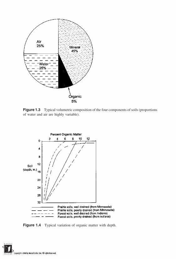
Figure 1.3 Typical volumetric composition of the four components of soils (proportionsof water and air are highly variable).

Figure 1.4 Typical variation of organic matter with depth.

Figure 1.5 Schematic representation of solid, water, and air phases in soil.

tively the relative proportions of the solid, water, and air phases. In accordancewith common practice, we will not make a distinction between the mineral matterand the organic matter in the solid phase. Figure 1.5 shows a schematic represen-tation of the three phases with their weights indicated on the left-hand side andthe corresponding volumes indicated on the right-hand side.

The volume-based indicators of phase composition are:

Void ratio, e, defined as the ratio of volume of void space (occupied byboth water and air) to volume of solids, or

e Vv

Vs

(1.1)

Porosity, n, defined as the ratio of volume of void space to total volumeof soil mass, or

n Vv

V(1.2)

Degree of saturation, S, defined as the ratio of volume of water to volumeof void space, or

S Vw

Vv

(1.3)

Volumetric water content, θ, defined as the ratio of volume of water tototal volume of soil mass, or

θ Vw

V(1.4)

Of the four, the void ratio and porosity describe the volumetric extent of the voidspace, and the degree of saturation and volumetric water content indicate therelative wetness of the soil. The weight-based indicators of phase compositionare:

Water content, w, defined as the ratio of weight of water to the weight ofsolids, or

w Ww

Ws

(1.5)

Unit weight, γ, defined as the weight per unit volume of soil mass, or

γ W

V(1.6)

Note that water content is defined both in terms of volumes [Eq. (1.4)] andin terms of weights [Eq. (1.5)]. The former is used in hydrology and soil science,whereas the latter is more commonly found in geotechnical engineering literature.Geotechnical engineers often find it useful to exclude the water phase, and definethe unit weight in terms of the weight of solid phase alone. One area where thisis commonly done is soil compaction, discussed later in this chapter. The unitweight is then called dry unit weight, and is given as

γd Ws

V(1.7)

Using specific gravity, Gs, of solids (defined as the ratio of unit weight ofsolids to unit weight of water), and the unit weights of soil mass (γ or γd) andwater (γw), it is possible to relate the volume-based and weight-based indicatorsof phase composition. With the aid of Figure 1.6, the following expressions canbe derived:

n e

1 e(1.8)

θ Wγd

γw

(1.9)

Se wGs (1.10)

Figure 1.6 Phase relationships.

S θn

(1.11)

γd γ

1 w(1.12)

γ (1 w)Gsγw

1 e(1.13)

γd Gsγw

1 e(1.14)

Expressions such as the above are useful in assessing the relative quantitiesof the solid, water, and air phases in soils.

1.3.1 Geotechnical Processes Controlling PhaseComposition

The phase composition of soils is highly variable and is controlled by both naturaland man-made processes. Two such processes well known to geotechnical engi-neers are consolidation and compaction. Consolidation is a process involvingreduction of void ratio as a result of load application on a soil mass, which iscompletely saturated with water. This is an important process that governs settle-ments of structures. Compaction involves reduction of void ratio as a result ofexpulsion of air phase, generally aimed at increasing the dry unit weight of a

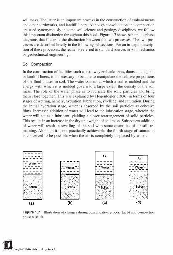
soil mass. The latter is an important process in the construction of embankmentsand other earthworks, and landfill liners. Although consolidation and compactionare used synonymously in some soil science and geology disciplines, we followthis important distinction throughout this book. Figure 1.7 shows schematic phasediagrams that illustrate the distinction between the two processes. The two pro-cesses are described briefly in the following subsections. For an in-depth descrip-tion of these processes, the reader is referred to standard sources in soil mechanicsor geotechnical engineering.

Soil Compaction

In the construction of facilities such as roadway embankments, dams, and lagoonor landfill liners, it is necessary to be able to manipulate the relative proportionsof the fluid phases in soil. The water content at which a soil is molded and theenergy with which it is molded govern to a large extent the density of the soilmass. The role of the water phase is to lubricate the solid particles and bringthem close together. This was explained by Hogentogler (1936) in terms of fourstages of wetting, namely, hydration, lubrication, swelling, and saturation. Duringthe initial hydration stage, water is absorbed by the soil particles as cohesivefilms. Increased addition of water will lead to the lubrication stage, wherein thewater will act as a lubricant, yielding a closer rearrangement of solid particles.This results in an increase in the dry unit weight of soil mass. Subsequent additionof water will result in swelling of the soil with some quantities of air still re-maining. Although it is not practically achievable, the fourth stage of saturationis conceived to be possible when the air is completely displaced by water.

Figure 1.7 Illustration of changes during consolidation process (a, b) and compactionprocess (c, d).

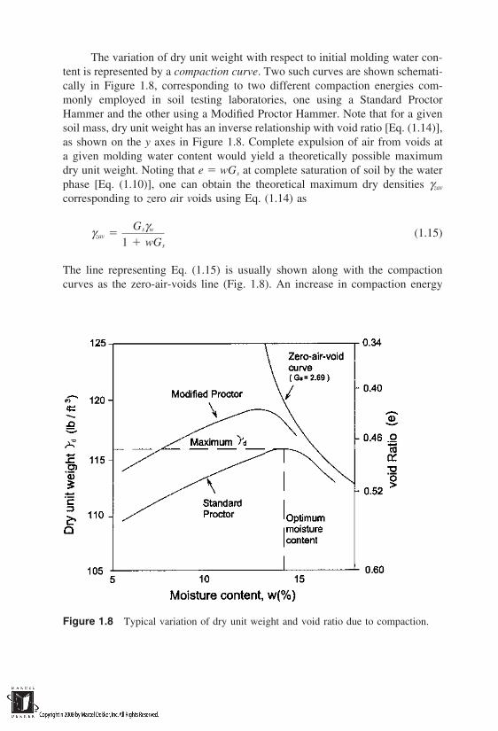
The variation of dry unit weight with respect to initial molding water con-tent is represented by a compaction curve. Two such curves are shown schemati-cally in Figure 1.8, corresponding to two different compaction energies com-monly employed in soil testing laboratories, one using a Standard ProctorHammer and the other using a Modified Proctor Hammer. Note that for a givensoil mass, dry unit weight has an inverse relationship with void ratio [Eq. (1.14)],as shown on the y axes in Figure 1.8. Complete expulsion of air from voids ata given molding water content would yield a theoretically possible maximumdry unit weight. Noting that e wGs at complete saturation of soil by the waterphase [Eq. (1.10)], one can obtain the theoretical maximum dry densities γzav

corresponding to zero air voids using Eq. (1.14) as

γzav Gsγw

1 wGs

(1.15)

The line representing Eq. (1.15) is usually shown along with the compactioncurves as the zero-air-voids line (Fig. 1.8). An increase in compaction energy

Figure 1.8 Typical variation of dry unit weight and void ratio due to compaction.

will result in higher dry unit weights, as one would expect; however, it is notpractically possible to remove all the air voids and achieve γzav in the field. In-crease in dry unit weight (or decrease in void ratio) and the associated changesin the skeleton of the soil mass play a crucial role in the fluid-transporting charac-teristics of compacted soils. This makes the soil compaction process very impor-tant in the context of waste-containment structures. The change in structure ofsoil as a result of compaction is discussed in detail in Chapter 2, and the changein fluid-transporting characteristics of compacted soils as a function of the com-paction variables (molding water content, compaction effort, etc.) is discussedin Chapter 3.

Soil Consolidation

In contrast to compaction process, consolidation involves expulsion of water witha consequent reduction in void ratio. Since the process involves travel of waterfrom a point of higher pressure to a point of lower pressure in soil, it is a time-dependent process. Depending on the type of soil, the thickness of the soil layer,and the magnitude of pressures developed in the pore water, the consolidationprocess may last several years or decades.

The magnitude of total void ratio reduction as a result of load applicationis often estimated by subjecting an in-situ soil sample to incremental loading inthe laboratory and obtaining a stress–strain relationship. The relationship is ob-tained in terms of effective stresses applied on the soil sample and void ratios,and is shown schematically in Figure 1.9. The effective stress is an indicator ofthe intergranular stress borne by the soil skeleton. It is obtained using Terzaghi’seffective stress principle, which states that the effective stress is the differencebetween total stress and pore water pressure. Once the slope of the consolidationcurve is known, the magnitude of void ratio reduction due to a given load increasecan be estimated. In general, two distinct slopes are exhibited in a consolidationcurve. Region I (Fig. 1.9) is marked by low void ratio reductions, indicating thatthe soil sample was compressed in the past under similar stresses. Region II ismarked by steep void ratio reductions, indicating that the soil sample is experienc-ing the stresses for the first time. The two regions meet at what is known aspreconsolidation pressure, pc, which is an indicator of the maximum pressure towhich the soil sample has ever been subjected in the past. A knowledge of thisparameter lets one track the history of the overburden stress at the site fromwhere the laboratory soil sample was obtained. The site is said to be normallyconsolidated if the current overburden stress po is equal to pc, or overconsolidatedif po is less than pc.

The change in void ratio ∆e for a given load increment ∆p may be obtainedas follows in terms of the slopes of consolidation curve Cc (compression index)and Cs (swell index).

Figure 1.9 Void ratio reduction due to consolidation process.

∆e Cc logpo ∆p

po for normally consolidated clays (1.16)

∆e Cs logpo ∆p

po

for overconsolidated clays when po ∆p pc (1.17)

∆e Cs logpc

po Cc logpo ∆p

pc

for overconsolidated clays when po ∆p pc (1.18)

The time rate at which void ratio is reduced during consolidation processis governed by a heat-conduction-type equation. This is dealt with in Chapter 3as a special case of groundwater flow.

1.4 SOLIDS COMPOSITION AND CHARACTERIZATION

We now narrow down our focus to the solid phase and study its composition interms of the nature and size of solid particles. Specifying the size of particles is

one of the common ways of characterizing the solid phase. However, becauseof the nature of weathering processes, the sizes of solid particles encountered inthe soil mass exhibit tremendous variation. Figure 1.10 illustrates the range ofsizes of particles grouped under the broad categories of sand, silt, and clay. Thereis at least a 100-fold difference between the sizes of sand and clay particles. Thecoexistence of particles of this vast size range obviously creates a variety of porespace architectures in soils, and hence the importance of a study of pore structuresin Chapter 2.

The size of particles was the original basis for grouping solids as sand, silt,and clay. A number of groupings have been developed over the years by variousorganizations. Figure 1.11 shows the groupings made by some of the major orga-nizations. The particle sizes imply equivalent diameters of spheres. It is alsocommon to characterize the solids under several subgroupings using the texturaltriangle (Fig. 1.12).

The experimental determination of particle sizes involves mechanical siev-ing for particles larger than 0.075 mm, and hydrometer analysis for particlessmaller than 0.075 mm. The mechanical sieving involves using sieves of knownmesh sizes to determine the fraction of solid particles passing through each sieve.The hydrometer analysis is based on the principle of sedimentation of soil parti-cles in water. Stokes’s law is used to relate the diameter D of particles (assumedto be spherical) to sedimentation velocity v.

v γs γw

18ηD2 (1.19)

Figure 1.10 Relative sizes of particles grouped under sand, silt, and clay.

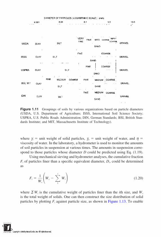
Figure 1.11 Groupings of soils by various organizations based on particle diameters(USDA, U.S. Department of Agriculture; ISSS, International Soil Science Society;USPRA, U.S. Public Roads Administration; DIN, German Standards; BSI, British Stan-dards Institute; and MIT, Massachusetts Institute of Technology).

where γs unit weight of solid particles, γw unit weight of water, and η viscosity of water. In the laboratory, a hydrometer is used to monitor the amountsof soil particles in suspension at various times. The amounts in suspension corre-spond to those particles whose diameter D could be predicted using Eq. (1.19).

Using mechanical sieving and hydrometer analyses, the cumulative fractionFi of particles finer than a specific equivalent diameter, Di, could be determinedas

Fi 1

WsWs

i

1

Wi (1.20)

where Wi is the cumulative weight of particles finer than the ith size, and Ws

is the total weight of solids. One can then construct the size distribution of solidparticles by plotting Fi against particle size, as shown in Figure 1.13. To enable

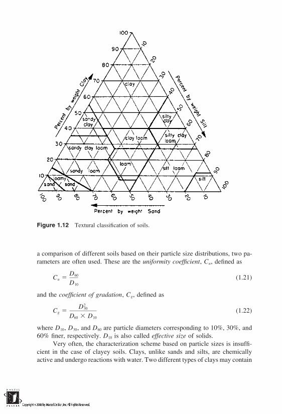
Figure 1.12 Textural classification of soils.

a comparison of different soils based on their particle size distributions, two pa-rameters are often used. These are the uniformity coefficient, Cu, defined as

Cu D60

D10

(1.21)

and the coefficient of gradation, Cg, defined as

Cg D2

30

D60 D10

(1.22)

where D10, D30, and D60 are particle diameters corresponding to 10%, 30%, and60% finer, respectively. D10 is also called effective size of solids.

Very often, the characterization scheme based on particle sizes is insuffi-cient in the case of clayey soils. Clays, unlike sands and silts, are chemicallyactive and undergo reactions with water. Two different types of clays may contain

Figure 1.13 Typical particle size distribution of soils.

particles of the same size range but react quite differently with water. They mayrequire different quantities of water to achieve the same consistency. At smallwater contents, the clayey soils behave as solids. As the water content is in-creased, they achieve semisolid and plastic stages, until a stage is reached wherethe water phase makes the solids behave like liquids. These stages were definedformally by Atterberg in the early 1900s in terms of what are now known asAtterberg limits. Simple experiments are routinely conducted in soil mechanicslaboratories to determine the water contents at which clayey soils pass throughthe various stages. Three limits are in general used to characterize the clayeysoils:

1. Shrinkage limit, which is the water content at which the soil passesfrom solid to semisolid state

2. Plastic limit, which is the water content at which transition from semi-solid to plastic state takes place

3. Liquid limit, which indicates the water content required in order forthe clayey soil to begin exhibiting flow characteristics like liquids

For simple procedures to determine these consistency limits in the labora-tory, the reader is referred to standard textbooks or laboratory manuals in geotech-nical engineering. It is in general accepted that the Atterberg limits are usefulindicators of the engineering behavior of soils. Several engineering properties ingeotechnical engineering are correlated to these limits. It is believed that thewater contents at which clayey soils transit from one state to the other representtheir entire physicochemical nature. The liquid limit, in particular, has been re-

cently established to be a state at which many of the properties are the samefor a variety of clay minerals. As we will see in the following section, differ-ent minerals need different quantities of water to bring them to the liquid limitstate. However, once they are at the liquid limit state, all the widely differingsoils seem to possess a relatively constant set of engineering properties suchas pore water suction, shear strength, and hydraulic conductivity (Nagaraj et al.,1994).

1.5 MINERAL COMPOSITION

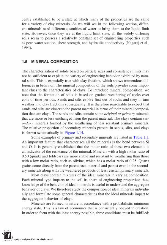
The characterization of solids based on particle sizes and consistency limits maynot be sufficient to explain the variety of engineering behavior exhibited by natu-ral soils. This is especially true with clay fraction, which shows tremendous dif-ferences in behavior. The mineral composition of the soils provides some impor-tant clues to the characteristics of clays. To introduce mineral composition, wenote that the formation of soils is based on gradual weathering of rocks overeons of time periods. Sands and silts evolve first out of rocks and they in turnweather into clay fractions subsequently. It is therefore reasonable to expect thatsands and silts are closer to the parent material in terms of their mineral composi-tion than are clays. The sands and silts contain some original or primary mineralsthat are more or less unchanged from the parent material. The clays contain sec-ondary minerals formed by the weathering of less resistant primary minerals.The relative proportion of secondary minerals present in sands, silts, and claysis shown schematically in Figure 1.14.

Some examples of primary and secondary minerals are listed in Table 1.1.An important feature that characterizes all the minerals is the bond between Siand O. It is generally established that the molar ratio of these two elements isan indicator of the resistance of the mineral. Minerals with a high molar ratio of0.50 (quartz and feldspar) are more stable and resistant to weathering than thosewith a low molar ratio, such as olivine, which has a molar ratio of 0.25. Quartzgrains come directly from the parent rock material and persist even in the second-ary minerals along with the weathered products of less resistant primary minerals.

Most clays contain mixtures of the ideal minerals in varying composition.Each mineral type imparts to the soil its share of engineering properties; thus,knowledge of the behavior of ideal minerals is useful to understand the aggregatebehavior of clays. We therefore study the composition of ideal minerals individu-ally and formulate some general characteristics that the ideal minerals impart tothe aggregate behavior of clays.

Minerals are formed in nature in accordance with a probabilistic minimumenergy state. This is a law of economics that is consistently obeyed in creation.In order to form with the least energy possible, three conditions must be fulfilled:

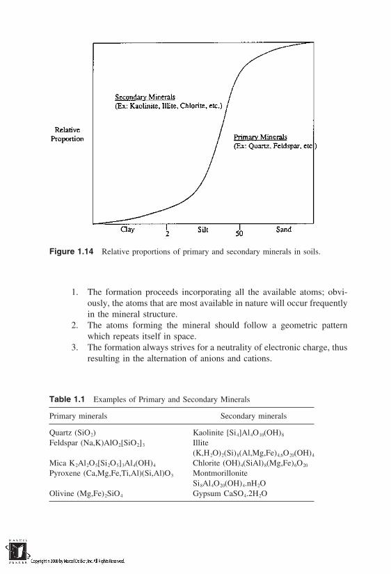
Figure 1.14 Relative proportions of primary and secondary minerals in soils.

1. The formation proceeds incorporating all the available atoms; obvi-ously, the atoms that are most available in nature will occur frequentlyin the mineral structure.

2. The atoms forming the mineral should follow a geometric patternwhich repeats itself in space.

3. The formation always strives for a neutrality of electronic charge, thusresulting in the alternation of anions and cations.

Table 1.1 Examples of Primary and Secondary Minerals

Primary minerals Secondary minerals

Quartz (SiO2) Kaolinite [Si4]Al4O10(OH)8

Feldspar (Na,K)AlO2[SiO2]3 Illite(K,H2O)2(Si)8(Al,Mg,Fe)4,6O20(OH)4

Mica K2Al2O5[Si2O5]3Al4(OH)4 Chlorite (OH)4(SiAl)8(Mg,Fe)6O20

Pyroxene (Ca,Mg,Fe,Ti,Al)(Si,Al)O3 MontmorilloniteSi8Al4O20(OH)4.nH2O

Olivine (Mg,Fe)2SiO4 Gypsum CaSO4.2H2O

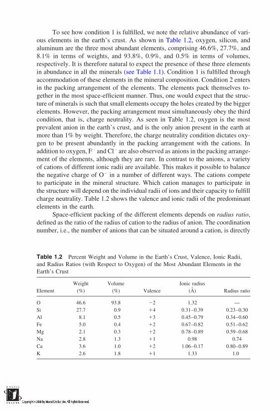
To see how condition 1 is fulfilled, we note the relative abundance of vari-ous elements in the earth’s crust. As shown in Table 1.2, oxygen, silicon, andaluminum are the three most abundant elements, comprising 46.6%, 27.7%, and8.1% in terms of weights, and 93.8%, 0.9%, and 0.5% in terms of volumes,respectively. It is therefore natural to expect the presence of these three elementsin abundance in all the minerals (see Table 1.1). Condition 1 is fulfilled throughaccommodation of these elements in the mineral composition. Condition 2 entersin the packing arrangement of the elements. The elements pack themselves to-gether in the most space-efficient manner. Thus, one would expect that the struc-ture of minerals is such that small elements occupy the holes created by the biggerelements. However, the packing arrangement must simultaneously obey the thirdcondition, that is, charge neutrality. As seen in Table 1.2, oxygen is the mostprevalent anion in the earth’s crust, and is the only anion present in the earth atmore than 1% by weight. Therefore, the charge neutrality condition dictates oxy-gen to be present abundantly in the packing arrangement with the cations. Inaddition to oxygen, F and Cl are also observed as anions in the packing arrange-ment of the elements, although they are rare. In contrast to the anions, a varietyof cations of different ionic radii are available. This makes it possible to balancethe negative charge of O in a number of different ways. The cations competeto participate in the mineral structure. Which cation manages to participate inthe structure will depend on the individual radii of ions and their capacity to fulfillcharge neutrality. Table 1.2 shows the valence and ionic radii of the predominantelements in the earth.

Space-efficient packing of the different elements depends on radius ratio,defined as the ratio of the radius of cation to the radius of anion. The coordinationnumber, i.e., the number of anions that can be situated around a cation, is directly

Table 1.2 Percent Weight and Volume in the Earth’s Crust, Valence, Ionic Radii,and Radius Ratios (with Respect to Oxygen) of the Most Abundant Elements in theEarth’s Crust

Weight Volume Ionic radiusElement (%) (%) Valence (A) Radius ratio

O 46.6 93.8 2 1.32 —Si 27.7 0.9 4 0.31–0.39 0.23–0.30Al 8.1 0.5 3 0.45–0.79 0.34–0.60Fe 5.0 0.4 2 0.67–0.82 0.51–0.62Mg 2.1 0.3 2 0.78–0.89 0.59–0.68Na 2.8 1.3 1 0.98 0.74Ca 3.6 1.0 2 1.06–0.17 0.80–0.89K 2.6 1.8 1 1.33 1.0

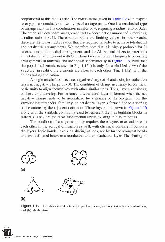
proportional to this radius ratio. The radius ratios given in Table 1.2 with respectto oxygen are conducive to two types of arrangements. One is a tetrahedral typeof arrangement with a coordination number of 4, requiring a radius ratio of 0.22.The other is an octahedral arrangement with a coordination number of 6, requiringa radius ratio of 0.41. These radius ratios are limiting values; in other words,these are the lowest radius ratios that are required in order to achieve tetrahedraland octahedral arrangements. We therefore note that it is highly probable for Sito enter into a tetrahedral arrangement, and for Al, Fe, and others to enter intoan octahedral arrangement with O. These two are the most frequently occurringarrangements in minerals and are shown schematically in Figure 1.15. Note thatthe popular schematic (shown in Fig. 1.15b) is only for a clarified view of thestructure; in reality, the elements are close to each other (Fig. 1.15a), with theanions hiding the cation.

A single tetrahedron has a net negative charge of -4 and a single octahedronhas a net negative charge of -10. The condition of charge neutrality forces thesebasic units to align themselves with other similar units. Thus, layers consistingof these units develop. For instance, a tetrahedral layer is formed when the netnegative charge tends to be neutralized by a sharing of the oxygens with thesurrounding tetrahedra. Similarly, an octahedral layer is formed due to a sharingof the anions by the adjacent octahedra. These layers are shown in Figure 1.16along with the symbols commonly used to represent them as building blocks inminerals. They are the most fundamental layers existing in clay minerals.

The condition of charge neutrality requires these layers to associate witheach other in the vertical dimension as well, with chemical bonding in betweenthe layers. Ionic bonds, involving sharing of ions, are by far the strongest bondsand are facilitated between a tetrahedral and an octahedral layer. The sharing of

(a)

(b)

Figure 1.15 Tetrahedral and octahedral packing arrangements: (a) actual coordination,and (b) idealization.

(a)

(b)

Figure 1.16 (a) Tetrahedral and (b) octahedral layers with symbolic notations.

anions at the interface of the two layers contributes to the charge neutrality. Suchstacking of layers results in the so-called subbasic or semibasic units. The nomen-clature used for the unit formed between one octahedral layer and one tetrahedrallayer is 1:1. Another important unit is formed when an octahedral layer is sand-wiched between two tetrahedral layers, with ionic bonds on either side of theoctahedral layer, and is represented as 2:1. These two subbasic units, shown inFigure 1.17, together constitute a majority of the minerals encountered in clays.

It is important to emphasize that because of the variety of cations availablein the earth, a number of different cations may be present in a given semibasicunit. The ionic radii of a number of cations (Table 1.2) are compatible enoughin size to form either a tetrahedral or an octahedral arrangement with anions. Forinstance, the tetrahedral layer may contain Al3 or Fe3 ions, and the octahedrallayer may contain Al3, Fe2, Zn, or Ni ions. Of course, such substitution takesplace with due regard to the condition of charge neutrality. When a trivalent ionsuch as Al3 occurs in an octahedral layer, no cation is observed in every thirdoctahedron, because of this condition of charge neutrality. Such substitution istermed isomorphous substitution and is common in a variety of minerals. Thelarge number of possibilities due to isomorphous substitution gives clays widelatitude of engineering behavior. Also, a number of possibilities arise for stackingof the two subbasic units either individually or in combination, thereby exhibitingwidely different engineering properties.

Before we outline the common mineral types, it is important to note that thecondition of charge neutrality may also be fulfilled in part by the liquid mediumsurrounding the subbasic units. An exchange of cations may result between thecation in the solution and the cation on the surface of the unit, thus altering thecharge balance. The total positive charge that a given mineral is capable of ad-

(a)

(b)

Figure 1.17 (a) 1:1 and (b) 2:1 subbasic units and their symbolic notations.

sorbing is equal to its net negative charge. This capacity of the mineral to adsorbcations is termed the cation-exchange capacity (CEC) of soils. It is expressed asmilliequivalents of cations adsorbed per 100 g of dry soil (mEq/100 g) which isequivalent to centimoles of positive charge per kilogram of dry soil. CEC is animportant property of the mineral that governs the interactions between solidsand the pore fluid.

The common minerals formed by the stacking of the subbasic units areshown in Figure 1.18. Some important properties of these minerals are listed inTable 1.3, and their characteristics are outlined briefly below.

Figure 1.18 Stacking of the subbasic units for some common minerals.

Kaolinite is formed by the stacking of 1:1 units with strong hydrogen bond-ing between O2 and OH of the tetrahedra and octahedra, respectively. Becauseof the strong bonding, kaolinite does not exhibit swelling in water. It is character-ized by a low surface area and low CEC.

Halloysite is similar to kaolinite in that it has 1:1 layer structure; however,

Table 1.3 Important Properties of Clay Minerals

Specific surface CEC Basal spacingMineral (m2/g) Specific gravity (mEq/100 g) (A)

Kaolinite 10–20 2.60–2.68 3–15 7.2Halloysite 35–70 2.00–2.20 5–40 10.1Illite 65–100 2.6–3.00 10–40 10Vermiculite 40–80 100–150 10.5–14Montmorillonite 700–840 2.35–2.70 80–150 9.6–infinityChlorite 80 2.6–2.96 10–40 14

it has a sheet of water molecules between the layers and therefore the thicknessof stacked units is greater. Upon dehydration, halloysite collapses irreversibly tokaolinite structure.

Illite is formed by the stacking of 2:1 units bonded together by potassiumions. The negative charge inviting potassium ions is due to the substitution ofaluminum for some silicon in the tetrahedral sheets. Illite’s structure is similarto that of the primary mineral mica, except that it is less crystalline and containsless potassium. The potassium ions, fixed between the layers, prevent swellingof the mineral and provide little interlayer surface area for cation exchange.

Vermiculite has a 2:1 layer structure similar to that of illite, but the subbasicunits in this case are separated by a couple of sheets of water molecules. Substitu-tion of aluminium for some silicon is found in this mineral also, resulting in ahigh net negative charge.

Montmorillonite is again a 2:1 layer structure, but with extensive isomor-phous substitution of magnesium and iron for aluminum in the octahedral sheets.Unlike illite, no potassium ions are found between the layers, and unlike vermicu-lite, the layers are separated by several sheets of water molecules. A distinguish-ing feature of this mineral is that it swells extensively when placed in waterbecause of the penetration of water molecules into the interlayer spacing. It isdue to this that the liquid limit of montmorillonites is very high.

Chlorite is often termed a 2:1:1 layer silicate because of the presence ofa metal hydroxide sheet sandwiched between 2:1 units. The interlayer sheet isoften known as a brucite layer, named after the mineral brucite, which has magne-sium as the cation in an octahedral arrangement. Some isomorphous substitutionof Mg2 by Al3 exists in this intermediate layer. Chlorite has low surface areaand CEC because of the presence of this layer, and it does not swell in water.

It must be emphasized that the composition of any single ideal mineraloutlined above is rarely exhibited in its entirety in a clay fraction. A number ofminerals are present in a given soil and one or more of these minerals may domi-nate the composition, but rarely does the soil exhibit the extreme character of anideal mineral. The successive layers may belong to different minerals. They maynot be bonded together in a way that can be generalized. These are called mixed-layer minerals and may have a predictable structure (such as every other layerbeing an illite or montmorillonite) or a totally random structure.

1.6 ROLE OF COMPOSITION IN ENGINEERING BEHAVIOROF SOILS

We observe in this section how the compositional aspects at various scales influ-ence the engineering properties of soils. The fundamental character or signatureof soils often lies in the mineral composition. For a given percentage of solids

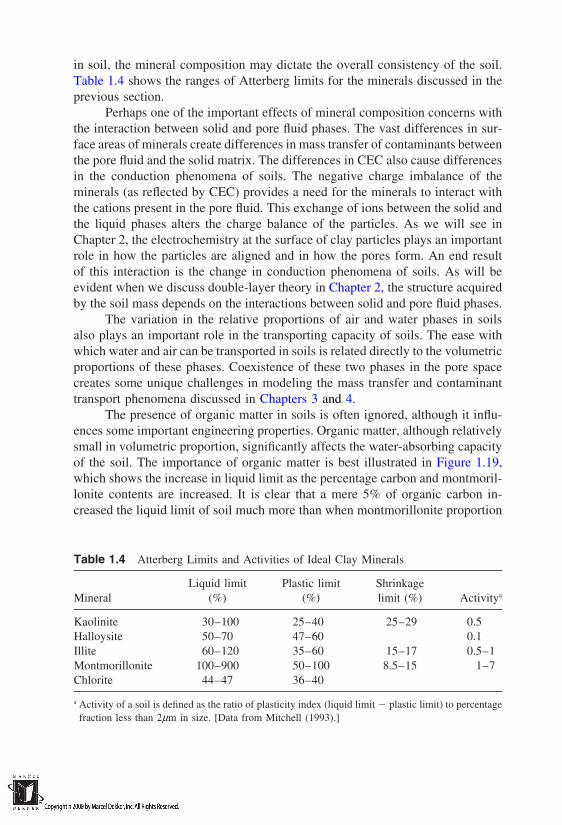
in soil, the mineral composition may dictate the overall consistency of the soil.Table 1.4 shows the ranges of Atterberg limits for the minerals discussed in theprevious section.

Perhaps one of the important effects of mineral composition concerns withthe interaction between solid and pore fluid phases. The vast differences in sur-face areas of minerals create differences in mass transfer of contaminants betweenthe pore fluid and the solid matrix. The differences in CEC also cause differencesin the conduction phenomena of soils. The negative charge imbalance of theminerals (as reflected by CEC) provides a need for the minerals to interact withthe cations present in the pore fluid. This exchange of ions between the solid andthe liquid phases alters the charge balance of the particles. As we will see inChapter 2, the electrochemistry at the surface of clay particles plays an importantrole in how the particles are aligned and in how the pores form. An end resultof this interaction is the change in conduction phenomena of soils. As will beevident when we discuss double-layer theory in Chapter 2, the structure acquiredby the soil mass depends on the interactions between solid and pore fluid phases.

The variation in the relative proportions of air and water phases in soilsalso plays an important role in the transporting capacity of soils. The ease withwhich water and air can be transported in soils is related directly to the volumetricproportions of these phases. Coexistence of these two phases in the pore spacecreates some unique challenges in modeling the mass transfer and contaminanttransport phenomena discussed in Chapters 3 and 4.

The presence of organic matter in soils is often ignored, although it influ-ences some important engineering properties. Organic matter, although relativelysmall in volumetric proportion, significantly affects the water-absorbing capacityof the soil. The importance of organic matter is best illustrated in Figure 1.19,which shows the increase in liquid limit as the percentage carbon and montmoril-lonite contents are increased. It is clear that a mere 5% of organic carbon in-creased the liquid limit of soil much more than when montmorillonite proportion

Table 1.4 Atterberg Limits and Activities of Ideal Clay Minerals

Liquid limit Plastic limit ShrinkageMineral (%) (%) limit (%) Activitya

Kaolinite 30–100 25–40 25–29 0.5Halloysite 50–70 47–60 0.1Illite 60–120 35–60 15–17 0.5–1Montmorillonite 100–900 50–100 8.5–15 1–7Chlorite 44–47 36–40

a Activity of a soil is defined as the ratio of plasticity index (liquid limit plastic limit) to percentagefraction less than 2µm in size. [Data from Mitchell (1993).]

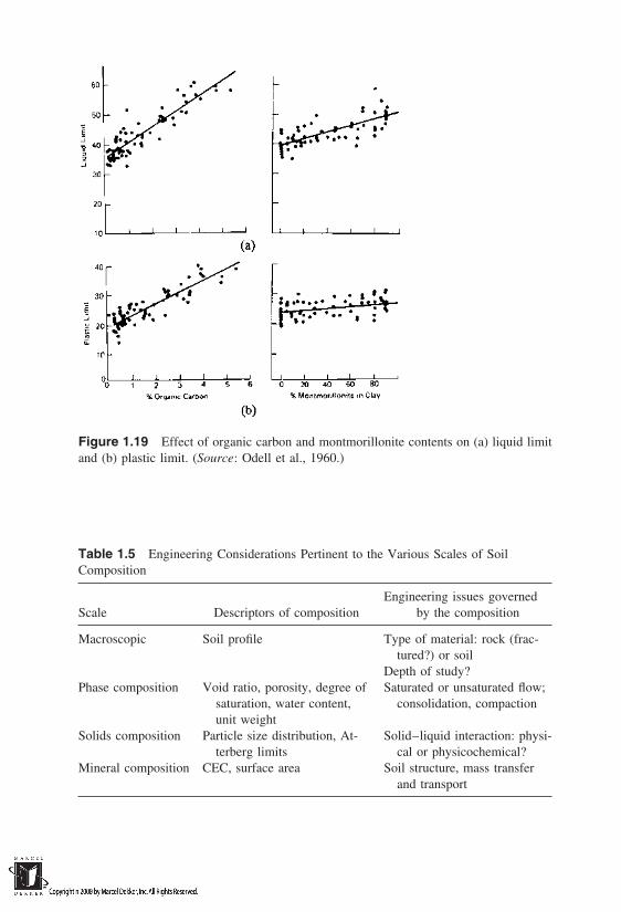
Figure 1.19 Effect of organic carbon and montmorillonite contents on (a) liquid limitand (b) plastic limit. (Source: Odell et al., 1960.)

Table 1.5 Engineering Considerations Pertinent to the Various Scales of SoilComposition

Engineering issues governedScale Descriptors of composition by the composition

Macroscopic Soil profile Type of material: rock (frac-tured?) or soil

Depth of study?Phase composition Void ratio, porosity, degree of Saturated or unsaturated flow;

saturation, water content, consolidation, compactionunit weight

Solids composition Particle size distribution, At- Solid–liquid interaction: physi-terberg limits cal or physicochemical?

Mineral composition CEC, surface area Soil structure, mass transferand transport

is increased up to 80%. The same effect is shown in plastic limit. In terms ofmechanical properties of soils, the organic matter is known to reduce the maxi-mum dry unit weight and cohesion of soils (Franklin et al., 1973). The cation-exchange capacity may increase significantly when organic matter is present insoils. Often, the organic matter accounts for 30–90% of the adsorbing capacityof minerals. On average, the cation-exchange capacity of the soil increases by 2mEq/100 g for each 1% of well-humified organic matter (Lyon et al., 1952).Organic matter is also a very good source of nutrients, an important considerationin bioremediation of contaminated sites.

Table 1.5 summarizes the important engineering issues governed by eachscale of soil composition. As we will see in the remaining chapters of the book,each scale is equally important in our consideration of practical geoenvironmentalissues.

REFERENCES

Arkley, R. J. (1964). Soil survey of the Eastern Stanislaus Area, California. U.S. Dept.Agr. and Cal. Agr. Exp. Sta.

Foth, H. D. (1990). Fundamentals of Soil Science, 8th ed. Wiley, New York.Franklin, A. F., Orozco, L. F., and Semrau, R. (1973). Compaction of slightly organic

soils. ASCE J. Soil Mech. Found. Div. 99 (SM7):541–557.Hogentogler, C. A. (1936). Essentials of soil compaction. Proc. Highway Research Board,

16:309.Jenny, H. (1941). Factors of Soil Formation; A System of Quantitative Pedology.

McGraw-Hill, New York.Lyon, T. L., Buckman, H. O., and Brady, N. C. (1952). The Nature and Properties of

Soils; A College Text of Edaphology. Macmillan, New York.McRae, S. G. (1988). Practical Pedology; Studying Soils in the Field. Ellis Horwood,

West Sussex, England.Mitchell, J. K. (1993). Fundamentals of Soil Behavior, 2nd ed. Wiley, New York.Nagaraj, T. S., Srinivasa Murthy, B. R., and Vatsala, A. (1994). Analysis and Prediction

of Soil Behavior. Wiley Eastern, New Delhi.Odell, R. T., Thornburn, T. H., and McKenzie, L. (1960). Relationships of Atterberg limits

to some other properties of Illinois soils. Proc. Soil Sci. Soc. Am., 24(5):297–300.

2Soil Structure

2.1 INTRODUCTION

As we have seen in Chapter 1, nature creates a large number of variations in soilcomposition during the stages of soil formation. When man-made variations dueto engineered processes (such as compaction) are added to these, the task ofdefining the physical appearance of soils becomes very difficult. The term fabricis commonly used to denote the physical arrangement of individual particles insoils. We will see shortly that identification of a ‘‘particle’’ is itself a matter ofjudgment in clays. Groups of single clay platelets aggregate to give an appearanceof what one may loosely call a particle. The term structure is used to denote notonly the physical arrangement within soils, as implied by ‘‘fabric,’’ but also itsstability or integrity. Yong and Sheeran (1973) define fabric as the ‘‘physicalarrangement of soil particles and includes the particle spacing and pore size distri-bution.’’ They define soil structure as ‘‘that property of the soil which providesfor its integrity.’’ In addition to the particle spacing and pore size distribution,the structure of soil encompasses the mineralogy and chemistry of the threephases that influence interparticle forces. Although the two terms, fabric andstructure, are often used synonymously, the distinction is important in the areaswhere the physical stability of soils is important. For instance, the sensitive natureof quick soils, collapsing and expanding soils, cannot be explained by mere con-sideration of fabric alone; the interplay of physicochemical forces between theparticles or particle groups must also be considered.

Most of the present conceptualizations of how soil particles group them-selves are based on observations using an optical or electron microscope. Figure2.1 shows, for instance, photomicrographs of six different materials at the samemagnification. Because of the subjective judgment involved in observing the pat-terns, the terminology associated with soil structure is quite extensive. Many ofthe terms are often used loosely, although their definitions are rigid elsewhere inother disciplines. An excellent example is the usage of flocculated and aggregated

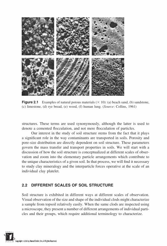
Figure 2.1 Examples of natural porous materials ( 10): (a) beach sand, (b) sandstone,(c) limestone, (d) rye bread, (e) wood, (f) human lung. (Source: Collins, 1961)

structures. These terms are used synonymously, although the latter is used todenote a cemented flocculation, and not mere flocculation of particles.

Our interest in the study of soil structure stems from the fact that it playsa significant role in the way contaminants are transported in soils. Porosity andpore-size distribution are directly dependent on soil structure. These parametersgovern the mass transfer and transport properties in soils. We will start with adiscussion of how the soil structure is conceptualized at different scales of obser-vation and zoom into the elementary particle arrangements which contribute tothe unique characteristics of a given soil. In that process, we will find it necessaryto study clay mineralogy and the interparticle forces operative at the scale of anindividual clay platelet.

2.2 DIFFERENT SCALES OF SOIL STRUCTURE

Soil structure is exhibited in different ways at different scales of observation.Visual observation of the size and shape of the individual clods might characterizea sample from topsoil relatively easily. When the same clods are inspected usinga microscope, they present a number of different arrangements of individual parti-cles and their groups, which require additional terminology to characterize.

Soil scientists whose primary focus is the root growth, tillage, and erosionin topsoils term the visible clods of the topsoils as aggregates. These aggregatesrange in size from millimeters to several centimeters. The U.S. Department ofAgriculture (USDA) arrived at a scheme to classify the structure of aggregatesbased on their size and shape. This classification scheme, shown in Table 2.1,uses primarily three descriptive terms to characterize the size and shape: platelike,prismlike, and blocklike. These three basic elements are shown in Figure 2.2.Platelike structure is one where horizontal axes are longer than vertical axes (Ein Fig. 2.2), whereas prismlike structure is one where vertical axes dominate.Pillarlike structure without round caps is termed prismatic (A) and with roundedcaps is termed columnar (B). Blocky structure is used to denote aggregate cubesup to 10 cm in size, with either angular (C) or subangular (D) planes. It alsoincludes smaller spheroids, which are further subdivided into crumbs, or granules(F) based on whether they appear to be porous or not.

Although the USDA classification of soil structure provides a simple wayto characterize the aggregates, it does not permit us to go to scales smaller thanthe visual size range. It is at small scales that soil structure plays its importantrole in altering the pore size distribution, and the chemical interactions betweenpore fluid and solid phase take place. Another difficulty associated with theUSDA classification is that it is truly not possible to affix an absolute size to anyvisible aggregate in the field because the aggregate can always be broken downto smaller groups of particles. The size distribution of the aggregates thereforedepends on the mechanical means used to separate them from one another.

This leads us to consider other characterizations of soil structure at smallerscales. Of the several conceptualizations that exist in the literature, the one pro-posed by Collins and McGown (1974) appears to be extensive. They studied thestructures exhibited by normally or lightly overconsolidated clays, silts, and sandsfrom a wide variety of geographic locations. These soils were associated withdifferent environments and depositional processes. Two distinct types of arrange-ments were apparent from these studies:

Type 1: Elementary particle arrangements consisting of single particles ofclay, silt, and sand

Type 2: Particle assemblages consisting of one or more forms of elementaryparticle arrangements or smaller particle assemblages

These two types of arrangements are associated with different scales ofpores, discussed later. Figure 2.3 shows a schematic of type 1 arrangements atparticle scale. It is very likely that a given soil exhibits more than one of thesearrangements side by side. An important observation that strengthens this charac-terization scheme is that soils of different environments and of different modesof deposition exhibited similar arrangements. Figure 2.4 shows a schematic oftype 2 arrangements, which are those of assemblages and are therefore of a

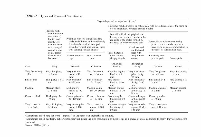
Table 2.1 Types and Classes of Soil Structure

Type (shape and arrangement of peds)

Blocklike; polyhedronlike, or spheroidal, with three dimensions of the same or-der of magnitude, arranged around a point

Platelike withone dimension Blocklike; blocks or polyhedrons(the vertical) having plane or curved surfaces that

Prismlike with two dimensions (thelimited and are casts of the molds formed byhorizontal) limited and considerably Spheroids or polyhedrone havinggreatly less the faces of the surrounding pedsless than the vertical; arranged plane or curved surfaces whichthan the otheraround a vertical line; vertical faces have slight or no accommodation totwo; arranged Mixed roundedwell defined; vertices angular the faces of surrounding peds.around a hori- and flattened

zontal plane; Faces flattened; faces withfaces mostly Without rounded With rounded most vertices many rounded Relatively non-horizontal caps caps sharply angular vertices porous peds Porous peds

(Anglular) SubangularClass Platy Prismatic Columnar blockya blockyb Granular Crumb

Very fine or very Very thin platy; Very fine pris- Very fine colum- Very fine angular Very fine suban- Very fine granu- Very fine crumb;thin 1 mm matic; 10 nar; 10 mm blocky; 5 gular blocky; lar; 1 mm 1 mm

mm mm 5 mmFine or thin Thin platy; 1 to 2 Fine prismatic; Fine columnar; Fine angular Fine subangular Fine granular; 1– Fine crumb; 1–2

mm 10–20 mm 10–20 mm blocky; 5–10 blocky; 5–10 2 mm mmmm mm

Medium Medium platy; Medium pris- Medium colum- Medium angular Medium subangu- Medium granular; Medium crumb;2–5 mm matic; 20–50 nar; 20–50 mm blocky; 10–20 lar blocky; 10– 2–5 mm 2–5 mm

mm mm 20 mmCoarse or thick Thick platy; 5– Coarse prismatic; Coarse columnar; Coarse angular Coarse subangu- Coarse granular;

10 mm 50–100 mm 50–100 mm blocky; 20–50 lar blocky; 20– 5–10 mmmm 50 mm

Very coarse or Very thick platy; Very coarse pris- Very coarse co- Very coarse angu- Very coarse sub- Very coarse gran-very thick 10 mm matic; 100 lumnar; 100 lar blocky; angular blocky; ular; 10 mm

mm mm 50 mm 50 mm

a Sometimes called nut; the word ‘‘angular’’ in the name can ordinarily be omitted.b Sometimes called nuciform, nut, or subangular nut. Since the size connotation of these terms is a source of great confusion to many, they are not recom-

mended.Source: USDA (1951).

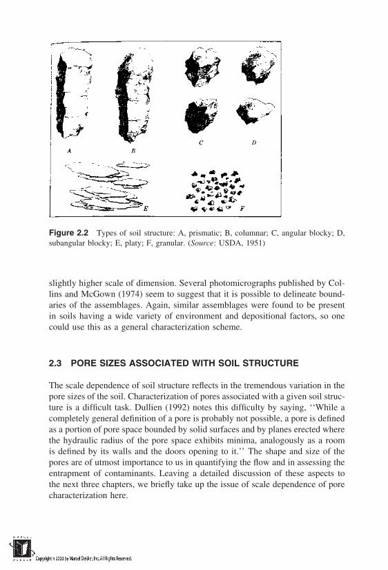
Figure 2.2 Types of soil structure: A, prismatic; B, columnar; C, angular blocky; D,subangular blocky; E, platy; F, granular. (Source: USDA, 1951)

slightly higher scale of dimension. Several photomicrographs published by Col-lins and McGown (1974) seem to suggest that it is possible to delineate bound-aries of the assemblages. Again, similar assemblages were found to be presentin soils having a wide variety of environment and depositional factors, so onecould use this as a general characterization scheme.

2.3 PORE SIZES ASSOCIATED WITH SOIL STRUCTURE

The scale dependence of soil structure reflects in the tremendous variation in thepore sizes of the soil. Characterization of pores associated with a given soil struc-ture is a difficult task. Dullien (1992) notes this difficulty by saying, ‘‘While acompletely general definition of a pore is probably not possible, a pore is definedas a portion of pore space bounded by solid surfaces and by planes erected wherethe hydraulic radius of the pore space exhibits minima, analogously as a roomis defined by its walls and the doors opening to it.’’ The shape and size of thepores are of utmost importance to us in quantifying the flow and in assessing theentrapment of contaminants. Leaving a detailed discussion of these aspects tothe next three chapters, we briefly take up the issue of scale dependence of porecharacterization here.

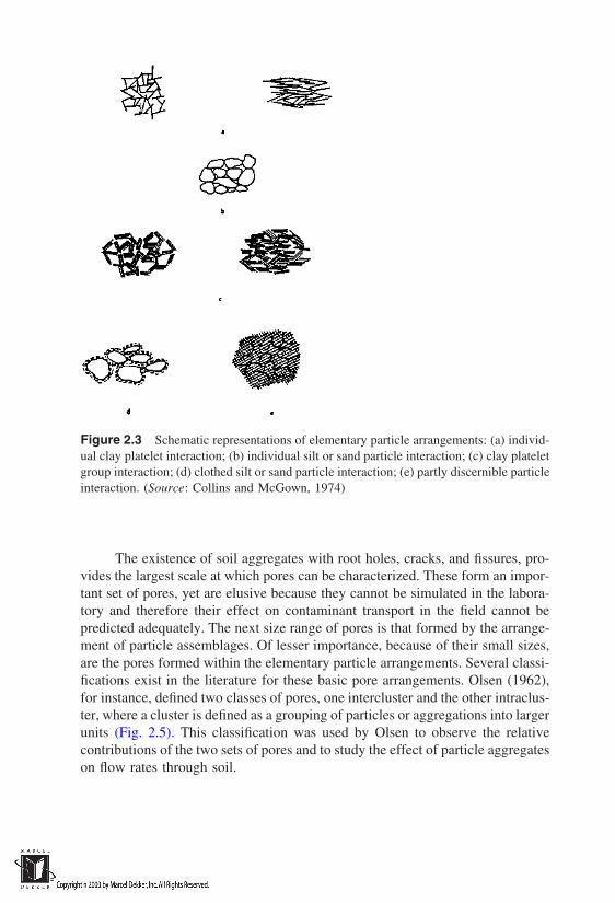
Figure 2.3 Schematic representations of elementary particle arrangements: (a) individ-ual clay platelet interaction; (b) individual silt or sand particle interaction; (c) clay plateletgroup interaction; (d) clothed silt or sand particle interaction; (e) partly discernible particleinteraction. (Source: Collins and McGown, 1974)

The existence of soil aggregates with root holes, cracks, and fissures, pro-vides the largest scale at which pores can be characterized. These form an impor-tant set of pores, yet are elusive because they cannot be simulated in the labora-tory and therefore their effect on contaminant transport in the field cannot bepredicted adequately. The next size range of pores is that formed by the arrange-ment of particle assemblages. Of lesser importance, because of their small sizes,are the pores formed within the elementary particle arrangements. Several classi-fications exist in the literature for these basic pore arrangements. Olsen (1962),for instance, defined two classes of pores, one intercluster and the other intraclus-ter, where a cluster is defined as a grouping of particles or aggregations into largerunits (Fig. 2.5). This classification was used by Olsen to observe the relativecontributions of the two sets of pores and to study the effect of particle aggregateson flow rates through soil.

Figure 2.4 Schematic representations of particle assemblages: (a) (b) (c) connectors;(d) irregular aggregations linked by connector assemblages; (e) irregular aggregationsforming a honeycomb arrangement; (f ) regular aggregations interacting with silt or sandgrains; (g) regular aggregation interacting with particle matrix; (h) interweaving bunchesof clay; ( j) interweaving bunches of clay with silt inclusions; (k) clay particle matrix; (l)granular particle matrix. (Source: Collins and McGown, 1974)

Collins and McGown (1974) provided another classification based on ob-servations of soil fabric discussed above. Four classes of pores were suggestedin that study:

1. Intraelemental pores occurring within the various elementary particlearrangements, including both interparticle pores and intergroup pores(those occurring between groups of clay plates)

2. Intraassemblage pores existing within particle assemblages or betweensmaller particle assemblages within a bigger assemblage

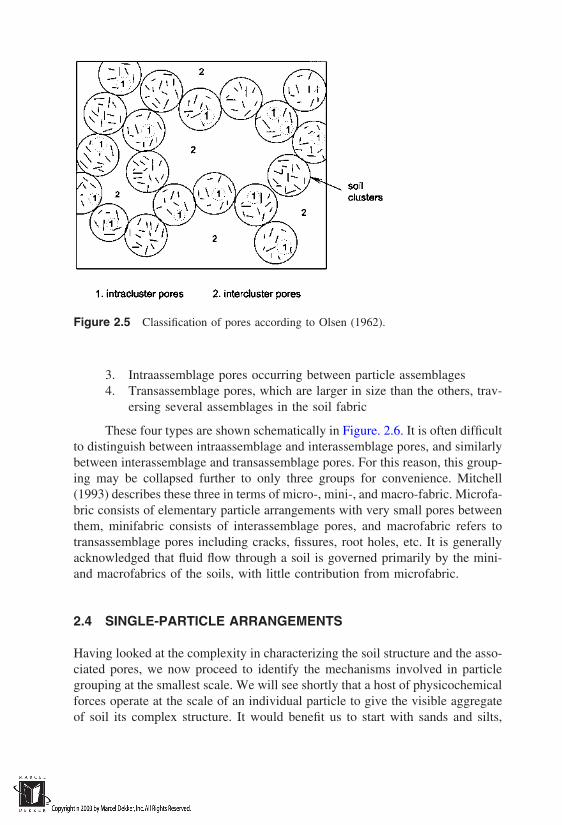
Figure 2.5 Classification of pores according to Olsen (1962).

3. Intraassemblage pores occurring between particle assemblages4. Transassemblage pores, which are larger in size than the others, trav-

ersing several assemblages in the soil fabric

These four types are shown schematically in Figure. 2.6. It is often difficultto distinguish between intraassemblage and interassemblage pores, and similarlybetween interassemblage and transassemblage pores. For this reason, this group-ing may be collapsed further to only three groups for convenience. Mitchell(1993) describes these three in terms of micro-, mini-, and macro-fabric. Microfa-bric consists of elementary particle arrangements with very small pores betweenthem, minifabric consists of interassemblage pores, and macrofabric refers totransassemblage pores including cracks, fissures, root holes, etc. It is generallyacknowledged that fluid flow through a soil is governed primarily by the mini-and macrofabrics of the soils, with little contribution from microfabric.

2.4 SINGLE-PARTICLE ARRANGEMENTS

Having looked at the complexity in characterizing the soil structure and the asso-ciated pores, we now proceed to identify the mechanisms involved in particlegrouping at the smallest scale. We will see shortly that a host of physicochemicalforces operate at the scale of an individual particle to give the visible aggregateof soil its complex structure. It would benefit us to start with sands and silts,

Figure 2.6 Schematic representation of pore space types. (Source: Collins andMcGown, 1974)

because their arrangements are far simpler than clays. Unlike in clays, there islittle chemical interaction in the particle arrangement of sands and silts.

The ways in which spherical grains of the same size can be packed arelimited in number. Because of the uniformity with which we can pack thesegrains, it is possible to predict mathematically the volume occupied by the porespace given the packing arrangement. Figure 2.7 shows five regular packing ar-rangements of equal spheres. The cubical arrangement shown in case (a) offersthe minimal density and maximum porosity, with a coordination number (pointsof contact per sphere) of 6 and a mean bulk porosity of 47.64%. Pyramidal andtetrahedral arrangements offer the densest states of packing, with a coordinationnumber of 12 and a mean bulk porosity of 25.95%. Table 2.2 shows the propertiesof intermediate regular packings.

Similar to regular packings, random packings were also found to be associ-ated with a characteristic range of porosities. For instance, Haughey and Bever-idge (1969) identified four random packing arrangements with narrow range ofporosities exhibited by each of the arrangements: (1) very loose random packingwith a porosity of about 0.44, obtained by slowly reducing the velocity in afluidized bed; (2) loose random packing with a porosity range of 0.40–0.41, ob-tained by individual random hand packing; (3) poured random packing with a

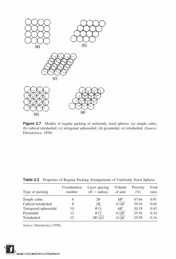
Figure 2.7 Models of regular packing of uniformly sized spheres: (a) simple cubic;(b) cubical tetrahedral; (c) tetragonal sphenoidal; (d) pyramidal; (e) tetrahedral. (Source:Deresiewicz, 1958)

Table 2.2 Properties of Regular Packing Arrangements of Uniformly Sized Spheres

Coordination Layer spacing Volume Porosity VoidType of packing number (R radius) of unit (%) ratio

Simple cubic 6 2R 8R3 47.64 0.91Cubical-tetrahedral 8 2R 4√3R3 39.54 0.65Tetragonal-sphenoidal 10 R√3 6R3 30.19 0.43Pyramidal 12 R√2 4√2R3 25.95 0.34Tetrahedral 12 2R√2/3 4√2R3 25.95 0.34

Source: Deresiewicz (1958).

porosity range of 0.375 to 0.391, when spheres are poured into a container; and(4) close random packing, with porosities of 0.359 to 0.375, obtained when thepacking is vibrated or shaken vigorously. In general, the coordination number isrepresentative of the fabric and may be used to infer the porosity. Ridgway andTarbuck (1967) give us a regression relationship between coordination numberu, and porosity n:

n 1.072 0.1193u 0.004312u2 (2.1)

Similar relationships exist in the literature between porosity and coordina-tion number. One has to be careful in applying these regression equations topolydisperse systems wherein the sphere size varies and therefore the relation-ships are far more complex. In general, the porosities of natural systems con-sisting of sands and silts of varying size lie within the theoretical limits of thepacking arrangements discussed above.

In the case of clays, the individual particle arrangement varies significantlybecause of the varied mineralogy of the particles and their rather complex associa-tion with the pore fluid. Early studies were focused on the particle arrangementsin suspensions only. Although there are additional factors to consider in real soilmasses, a knowledge of particle arrangement in clay suspensions is an importantfirst step in understanding the structure of clays. Figure 2.8 shows the possibleassociations between clay particles in suspensions. The terminology associatedwith these associations is as follows.

Dispersed: No face-to-face association between particles exists.Aggregated: Face-to-face association of several particles exists.Flocculated: Edge-to-face or edge-to-edge association of particles exists.Deflocculated: No edge-to-face or edge-to-edge association between parti-

cles exists.

An understanding of the factors responsible for various associations shownin Fig. 2.8 is essential in order to at least qualitatively predict the structurechanges of clays due to environmental factors. This takes us to a study of clay–water interactions because the individual particle arrangement of clay particlesoccurs through the medium of water films attracted to clay particles. The twoprimary mechanisms for attraction between clays and water are that (1) the dipo-lar nature of water molecules brings the molecules close to the negatively chargedclay particles, and (2) any cations existing in the vicinity of the clay particle tendto be attracted to the clay particles, bringing with them the water of hydration.Mitchell (1993) subdivides these into four specific mechanisms (Fig. 2.9):

1. Hydrogen bonding between the hydrogen of water molecules and theoxygen or hydroxyl of clay particle surfaces

2. Hydration of cations in the vicinity of the clay particles

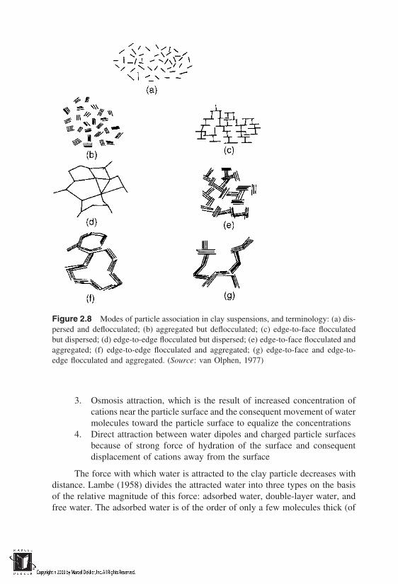
Figure 2.8 Modes of particle association in clay suspensions, and terminology: (a) dis-persed and deflocculated; (b) aggregated but deflocculated; (c) edge-to-face flocculatedbut dispersed; (d) edge-to-edge flocculated but dispersed; (e) edge-to-face flocculated andaggregated; (f) edge-to-edge flocculated and aggregated; (g) edge-to-face and edge-to-edge flocculated and aggregated. (Source: van Olphen, 1977)

3. Osmosis attraction, which is the result of increased concentration ofcations near the particle surface and the consequent movement of watermolecules toward the particle surface to equalize the concentrations

4. Direct attraction between water dipoles and charged particle surfacesbecause of strong force of hydration of the surface and consequentdisplacement of cations away from the surface

The force with which water is attracted to the clay particle decreases withdistance. Lambe (1958) divides the attracted water into three types on the basisof the relative magnitude of this force: adsorbed water, double-layer water, andfree water. The adsorbed water is of the order of only a few molecules thick (of

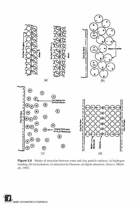
Figure 2.9 Modes of attraction between water and clay particle surfaces: (a) hydrogenbonding; (b) ion hydration; (c) attraction by Osmosis; (d) dipole attraction. (Source: Mitch-ell, 1993)

the order of 10 A) held by strong forces—so strong that it takes about 10,000atmospheres to pull the water molecules off the surface. The double-layer water,which is often lumped with adsorbed water in some classification terminologies,is attracted by less strong forces, which make it easy for flow to take place parallelto the particle surface but make it difficult to pull the water without subsequentreplacement. Obviously, the thicknesses of these layers depend on the chargedensity of the particle surfaces, among other parameters. The higher the chargedensity, the higher is the thickness of these layers, and vice versa. Figures 2.10aand 2.10b demonstrate this dependency of the thickness of water layers on thecharge density. It is seen that kaolinite, by virtue of its high charge density, pos-sesses a thicker water layer than montmorillonite. This should not lead us toconclude that the water content of montmorillonite systems is lower than thoseof kaolinite. Quite the contrary is true, because the specific surface area of mont-morillonite is far greater than that of kaolinite. Consideration of the double layeris quite important in soil systems, since most pore water in field soils is containedin that layer.

Contact between individual particles takes place through the water layers.The interaction of forces of the water layers of two approaching particles, coupledwith externally applied forces and environmental changes, governs the particlearrangement. Whether two mineral surfaces ever come into physical contact isstill an issue of controversy. However, a knowledge of the various factors affect-ing the forces of attraction and repulsion between two particles is needed to un-

Figure 2.10 Comparison of water layer thicknesses: (a) montmorillonite crystal; (b)kaolinite crystal. (Source: Lambe, 1958)

derstand the environmental influences of particle arrangement. Theoretical treat-ment of the double layer based on electrostatics provides us with this knowledge.

2.5 GOUY-CHAPMAN THEORY OF THE DOUBLE LAYER

Gouy (1910) and Chapman (1913) independently arrived at a theoretical expres-sion for electric potential in the double layer, which enables us to look at theeffect of various characteristics of the medium on the thickness of the layer.The theory invokes and combines two well-known equations, one expressing thevariation of electric potential with respect to distance known as the Poisson equa-tion, and the other describing the relationship between ion distribution and elec-tric potential known as the Boltzmann equation.

The Poisson equation indicates that the electric potential ψ decreases asthe distance from the source, i.e., a clay particle surface with a negative electricpotential, increases. The presence of charges or ions, and the dielectric constantof the medium, govern this decrease in potential. The equation is commonlyexpressed as

d2ψdx2

4πρ

(2.2)

where x distance from the source; ρ charge density; and dielectricconstant of the medium. The charge density in the medium is the contributionof the anions and cations in the medium,

ρ c(vn vn) (2.3)

where c electronic charge; v valency; n number of ions per unit volume,and the and subscripts indicate cations and anions, respectively. The numberof ions in Eq. (2.3) is itself governed by the electric potential ψ. The Boltzmannequation provides us with the relationship between the two for cations and anions:

n n0e(vcψ/kT) (2.4)

n n0e(vcψ/kT) (2.5)

where n0 density of ions far away from the surface, k Boltzmann constant(1.38 1023 J K1), and T temperature in kelvins. For a clay particle, thepotential ψ is negative; therefore, the cation population increases and the anionpopulation decreases as the negative potential is increased. Considering that thepotential ψ decreases with distance from the charged clay surface, the distribution

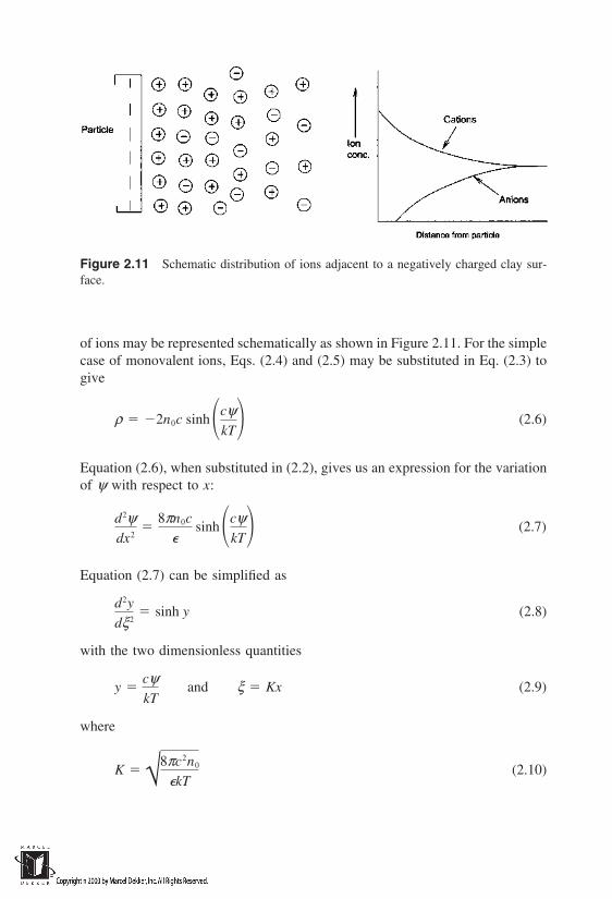
Figure 2.11 Schematic distribution of ions adjacent to a negatively charged clay sur-face.

of ions may be represented schematically as shown in Figure 2.11. For the simplecase of monovalent ions, Eqs. (2.4) and (2.5) may be substituted in Eq. (2.3) togive

ρ 2n0c sinhcψkT (2.6)

Equation (2.6), when substituted in (2.2), gives us an expression for the variationof ψ with respect to x:

d2ψdx2

8πn0c

sinhcψ

kT (2.7)

Equation (2.7) can be simplified as

d2y

dξ2 sinh y (2.8)

with the two dimensionless quantities

y cψkT

and ξ Kx (2.9)

where

K √8πc2n0

kT(2.10)

We now seek a particular solution for Eq. (2.8) for two specific boundaryconditions, one at the surface of the particle and the other at infinite distancefrom the particle. These conditions can be expressed as

y 0 anddy

dξ 0 at ξ ∞ (2.11)

and

y z eψ0

kTat ξ 0 (2.12)

where the potential at the surface of the particle is taken to be ψ0. For theseboundary conditions, the solution of Eq. (2.8) could be written as (Verwey andOverbeek, 1948)

ey/2 ez/2 1 (ey/2 1)eξ

ez/2 1 (ey/2 1)eξ(2.13)

Equation (2.13) implies an exponential decay of potential, decreasing from y z (ψ ψ0) at the surface of the particle to y 0 (ψ 0) at infinite distancefrom the particle surface. Several simplifications can be made to this solution fora number of special cases, as discussed by Verwey and Overbeek (1948). Threepopular simplifications are for the cases of z 1, z infinity, and ξ 1. Forthese cases, the solutions may be obtained as

ψ ψ0eKx for z 1 (2.14)

ψ 2kT

eln coth

Kx

2for z ∞ (2.15)

and

ψ 4kT

e ez/2 1ez/2 1eξ for arbitrary z and ξ 1 (2.16)

Equation (2.14) is often referred as the Debye-Huckel equation, and 1/K repre-sents the characteristic length or thickness of the double layer (also known asthe Debye length). With the known electric potentials, the ion distributions maynow be obtained using Eqs. (2.4) and (2.5).

The Gouy-Chapman theory may be extended for the case of two interactingdouble layers when two clay surfaces approach each other. This case is shown

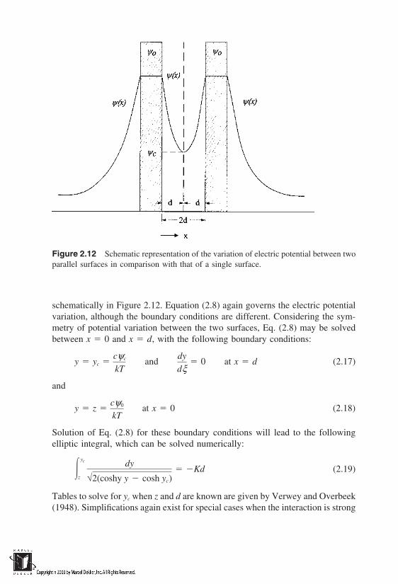
Figure 2.12 Schematic representation of the variation of electric potential between twoparallel surfaces in comparison with that of a single surface.

schematically in Figure 2.12. Equation (2.8) again governs the electric potentialvariation, although the boundary conditions are different. Considering the sym-metry of potential variation between the two surfaces, Eq. (2.8) may be solvedbetween x 0 and x d, with the following boundary conditions:

y yc cψc

kTand

dy

dξ 0 at x d (2.17)

and

y z cψ0

kTat x 0 (2.18)

Solution of Eq. (2.8) for these boundary conditions will lead to the followingelliptic integral, which can be solved numerically:

yc

z

dy

√2(coshy y cosh yc) Kd (2.19)

Tables to solve for yc when z and d are known are given by Verwey and Overbeek(1948). Simplifications again exist for special cases when the interaction is strong

(i.e., yc 1), and when the interaction is weak. The latter case in particularlends itself to a very simple solution. The electric potential at the midplane canbe approximated in that case as the summation of the electric potentials (y′c) dueto the two unperturbed double layers calculated separately. Thus,

yc 2y′c (2.20)

For weak interactions, ξ is necessarily large. Therefore Eq. (2.16) may be usedto calculate y′c for an individual double layer at a distance d. Substituting (2.16)in (2.20),

yc 8eKd ez/2 1ez/2 1

(2.21)

Langmuir (1938) provided yet another simplification for obtaining mid-plane potential assuming that the particle surfaces are so close that no anions arepresent between them and the potential at the particle surface is infinity. For theseconditions, his solution is

yc 2 lnπ

Kd(2.22)

This relatively simple solution compares well with the accurate solution in (2.19)beyond yc 1. For yc values less than 1, Eq. (2.21) may be used.

2.6 FORCES OF INTERACTION BETWEEN CLAYPARTICLES

The Gouy-Chapman theory discussed in the previous section describes the elec-tric potential variation and the ion distribution in the diffuse double layers, al-though with ideal configurations. The arrangement of the particles will now de-pend on how the particles repel or attract each other through these double layers.It is now necessary to relate the results of the Gouy-Chapman theory to forcesof interaction between the particles. Because of the like nature of surface charges,the forces due to diffuse double layers are repulsive. The forces of interactionbetween two charged surfaces in an electrolyte can be understood in terms ofthe increase in pressure as the two surfaces are brought together from infinity(at which instance the pressure is zero) to a separation distance of D. The increasein pressure depends on the ion density at the midplane and is given by the contactvalue theorem as (Israelachvili, 1992)

P(D) kT[ρc(D) ρc(∞)] (2.23)

where P(D) pressure between the surfaces when the two surfaces are separatedby a distance D, and ρc(D) and ρc(∞) ion densities at the midplane, when thetwo surfaces are separated by D and infinity, respectively.

To demonstrate the calculation of pressure between charged surfaces, letus take the case of a simple 1:1 electrolyte such as NaCl. Equation (2.6) can beused to obtain charge densities in terms of electric potentials at the midplane,ψc. Assuming that the midplane potential is zero when the two surfaces are sepa-rated by infinity, and considering both cations and anions, Eq. (2.23) may beexpressed by

P(D) kTn0[(ecψc/kT 1) (ecψc/kT 1)] (2.24)

which can be approximated as

P(D) n0c2ψ 2c

kT(2.25)

Using the result from Eq. (2.21) for ψc, which is valid when the interaction be-tween the surfaces is weak, and noting that D 2d, P(D) may be obtained as

P(D) 64kTn0eKD tan2 hcψ0

4kT (2.26)

The interaction between two particles is often expressed in terms of energy perunit area WR, the numerical value of which is simply the pressure integrated withrespect to D. Thus,

WR(D) 64kTn0eKD

Dtan2 hcψ0

4kT (2.27)

The repulsive energy due to double layers is not the only energy actingwhen two parallel charged surfaces approach each other. There are attractiveforces, called van der Waals forces, between any two surfaces due to the mutualinfluencing of the electronic motion of atoms on the two surfaces. The fluctuatingcharges due to the orbital movement of electrons causes instantaneous electricmoment and the resulting attraction between the two surfaces. For two parallelplates of thickness δ separated by a distance 2d, the attractive energy due to vander Waals forces, WA, is expressed as

WA A

48π 1d2

1

(d δ )2

2(d δ/2)2 (2.28)

where A is known as the Hamaker constant and is of the order of 1020 J. WA isoften approximated for certain limiting dimensions of d and δ. The approximateenergies for the limiting cases are

WA δ 2A

32πd4for d δ (2.29)

WA A

48π 1d2

7δ 2 for d δ (2.30)

WA A

48πd2for d δ (2.31)

The resultant of the repulsive (2.27) and attractive (2.28) energies governsthe particle arrangement. Because of the inverse relationship to the power of d,van der Waals forces of attraction diminish rapidly as the particle spacing in-creases. Other kinds of energies, such as those termed Born repulsion, may beoperative when the distances d are reduced to the order of an atomic diameter,which prevent interpenetration of the two surfaces. We do not have to be con-cerned with separations of this order, since for the most part, the particle separa-tions are such that double-layer repulsive and van der Waals attractive energiesare dominant.

The net repulsive/attractive force that is operative as the distance betweentwo charged particles is varied is often described quantitatively using DLVOtheory, after Derjaguin and Landau (1941), and Verwey and Overbeek (1948).This theory outlines the various stages of interaction between two particles, asshown schematically in Figure 2.13. Depending on the concentration of the elec-trolyte and the electric potential of particle surfaces, the particles may attracteach other at certain distances of separation and may repel each other at otherdistances. Figure 2.13a shows two peaks of the total interaction energy, one onthe repulsion side and the other on the attraction side. The peak on the repulsionside at a particle separation distance of d1 (typically of the order of 1–4 nm inmost systems) represents the energy barrier, which has to be crossed in orderfor particle surfaces to be attracted. The magnitude of this peak is significant forsystems with thick diffuse layers associated with highly charged surfaces andelectrolytes of low concentrations. Beyond the distances representing the energybarrier, weak attractive forces may be present, which are referred as secondaryminima (to distinguish them from the primary minima occurring much closer tothe particle surfaces). These are prominent in systems with concentrated electro-lyte systems. Many times, the particle separation distances are such that the en-ergy barrier is not crossed, and the particles are attracted to each other by weakforces corresponding to these secondary minima. Clay particles often flocculate

Figure 2.13 Schematic profiles of energy versus distance: (a) DLVO particle interactionenergies as the distance between two particles is varied; (b) effects of salt concentrationand particle surface potential on interaction energy.

in a slurry because of these weak forces. Upon slight disturbance such as shaking,the attractive forces are easily overcome and the particles are dispersed back.

Figure 2.13b shows the possible interaction curves between the particlesurfaces. With particles of weak interaction such as in the cases of low electricpotential and high salt concentrations, the energy barrier will become weak too.Thus a ‘‘stable’’ suspension of particles slowly begins to flocculate (from ‘‘a’’to ‘‘b’’). A situation may arise when the concentrations of the electrolyte reach‘‘critical coagulation concentrations’’ beyond which repulsive barrier disappears(‘‘c’’ and ‘‘d’’) and particles begin to flocculate rapidly.

It is apparent from the above discussion that quantitative analysis of inter-particle forces is possible to a certain extent when we idealize the clay particlesas parallel plates with their surface charge and the media properties known. In arealistic system, the forces of interaction may be due not only to particle surfacesapproaching each other, but also to the particle edges being exposed. For instance,the edges of the particles may expose cations and exhibit double layers containinga swarm of anions. It is therefore possible that double-layer attractive energiesprevail in the system between particle edges and surfaces. Quantitative analysesof these forces are also possible using the same general concepts outlined above.However, the uncertainties associated with the magnitudes of charge density onthe particle surfaces and edges, and the possible presence of foreign bondingmaterials between particles, make such analyses less attractive. Organic matterpresent in the system and certain nonclay materials such as iron oxide, aluminiumoxide, and carbonates bond to surfaces of one or more clay particles. These mate-

rials participate in bonding via either the stronger chemical bonds or by the vander Waals forces. Forces of bonding due to these cementing agents do not lendthemselves to a thorough quantitative analysis at a particle-scale level.

It is also important to know that several differences exist between the clayparticle systems in slurry form and the intact soil masses. Soil masses are rarelycomprised of a single mineral. The interacting particles may belong to differentminerals and as such may not conform to the ideal parallel-plate arrangement.The electric potentials of the particles may also vary significantly. The presenceof silt and sand particles embedded within the fine particle matrix poses additionalchallenges, since the colloidal principles do not apply to those particles. In spiteof these limitations, the theories explained above provide us a theoretical basisto judge qualitatively the impact of varying a given system parameter on theparticle arrangement and on the soil structure.

2.7 STRUCTURE VARIATIONS DUE TO CONSOLIDATIONAND COMPACTION

An external force applied to a fine-grained soil system acts against the repulsiveforces between the particles and tends to reduce the average spacing betweenthe particles. Although consolidation and compaction involve application of anexternal load, an important difference exists between the two processes in termsof the amount of water present in the system. In the case of consolidation, areduction in void volume takes place under saturated conditions. The particlerearrangement during the pore space reduction process is in general conceptual-ized as shown in Figure 2.14. To accommodate a reduced void ratio, an increasedorientation of clay particles takes place. From an open flocculated structure in-volving edge-to-face contacts at A, the structure changes to an increased face-to-face arrangement at B. Continued application of load will result in state C,where all clay particles are oriented face to face.

It is questionable whether a load of sufficient magnitude can ever be appliedto a soil mass so that the repulsive forces existing between particles can be over-come completely and the particles can be brought to physical contact. The distri-bution of force from the sample level to the particle level is difficult to assessbecause of the intricate structure of the soil mass. Indirect attempts were made tostudy how the pores become compressed as the consolidation stress is increased.Griffiths and Joshi (1989) observed, using mercury porosimetry, the changes inpore size distributions of clays at various stages of consolidation starting fromthe liquid limit state. The volume intruded by mercury represents the volume ofthe pore space. Figure 2.15 shows how the volume of the pore space occupiedby pores of various sizes changed as the consolidation stress is increased. Withreference to the liquid limit state, an increase in consolidation stress led to a

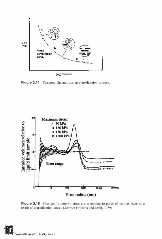
Figure 2.14 Structure changes during consolidation process.

Figure 2.15 Changes in pore volumes corresponding to pores of various sizes as aresult of consolidation stress. (Source: Griffiths and Joshi, 1989)

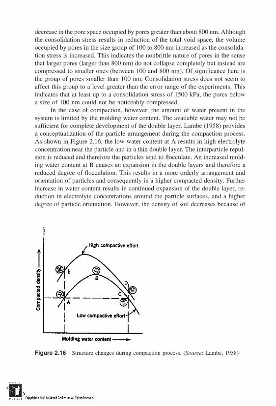
decrease in the pore space occupied by pores greater than about 800 nm. Althoughthe consolidation stress results in reduction of the total void space, the volumeoccupied by pores in the size group of 100 to 800 nm increased as the consolida-tion stress is increased. This indicates the nonbrittle nature of pores in the sensethat larger pores (larger than 800 nm) do not collapse completely but instead arecompressed to smaller ones (between 100 and 800 nm). Of significance here isthe group of pores smaller than 100 nm. Consolidation stress does not seem toaffect this group to a level greater than the error range of the experiments. Thisindicates that at least up to a consolidation stress of 1500 kPa, the pores belowa size of 100 nm could not be noticeably compressed.

In the case of compaction, however, the amount of water present in thesystem is limited by the molding water content. The available water may not besufficient for complete development of the double layer. Lambe (1958) providesa conceptualization of the particle arrangement during the compaction process.As shown in Figure 2.16, the low water content at A results in high electrolyteconcentration near the particle and in a thin double layer. The interparticle repul-sion is reduced and therefore the particles tend to flocculate. An increased mold-ing water content at B causes an expansion in the double layers and therefore areduced degree of flocculation. This results in a more orderly arrangement andorientation of particles and consequently in a higher compacted density. Furtherincrease in water content results in continued expansion of the double layer, re-duction in electrolyte concentrations around the particle surfaces, and a higherdegree of particle orientation. However, the density of soil decreases because of

Figure 2.16 Structure changes during compaction process. (Source: Lambe, 1958)

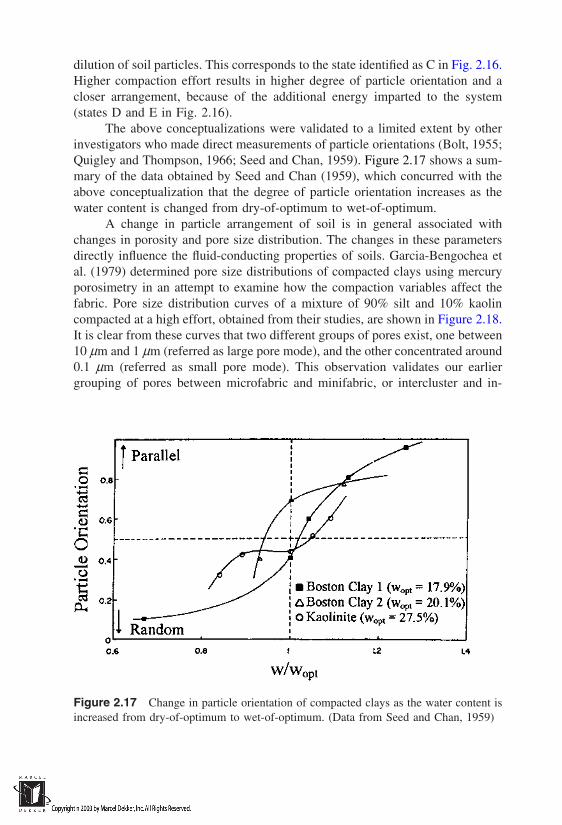
dilution of soil particles. This corresponds to the state identified as C in Fig. 2.16.Higher compaction effort results in higher degree of particle orientation and acloser arrangement, because of the additional energy imparted to the system(states D and E in Fig. 2.16).

The above conceptualizations were validated to a limited extent by otherinvestigators who made direct measurements of particle orientations (Bolt, 1955;Quigley and Thompson, 1966; Seed and Chan, 1959). Figure 2.17 shows a sum-mary of the data obtained by Seed and Chan (1959), which concurred with theabove conceptualization that the degree of particle orientation increases as thewater content is changed from dry-of-optimum to wet-of-optimum.

A change in particle arrangement of soil is in general associated withchanges in porosity and pore size distribution. The changes in these parametersdirectly influence the fluid-conducting properties of soils. Garcia-Bengochea etal. (1979) determined pore size distributions of compacted clays using mercuryporosimetry in an attempt to examine how the compaction variables affect thefabric. Pore size distribution curves of a mixture of 90% silt and 10% kaolincompacted at a high effort, obtained from their studies, are shown in Figure 2.18.It is clear from these curves that two different groups of pores exist, one between10 µm and 1 µm (referred as large pore mode), and the other concentrated around0.1 µm (referred as small pore mode). This observation validates our earliergrouping of pores between microfabric and minifabric, or intercluster and in-

Figure 2.17 Change in particle orientation of compacted clays as the water content isincreased from dry-of-optimum to wet-of-optimum. (Data from Seed and Chan, 1959)

Figure 2.18 Differential pore size distribution curves for 90% silt and 10% kaolin com-pacted at high effort. (Source: Garcia-Bengochea et al., 1979)

tracluster. It may be seen in Figure 2.18 that the small pore mode is relativelythe same at all states of compaction, and it is the large pore mode position andfrequency that seem to change with compaction. Garcia-Bengochea et al. (1979)indicate that in general, the position and the frequency of the large pore modeare the best indicators of the change in soil fabric caused by varying moldingwater content and compactive effort for a given soil type. It was also establishedthat the large pore mode controls the fluid conducting nature of the soil. There-fore, the change in soil structure must be an important consideration in any studydealing with fate and transport of contaminants in compacted soils.

2.8 ROLE OF SOIL STRUCTURE IN THE ENGINEERINGBEHAVIOR OF SOILS

Soil structure, by virtue of its influence on pore size distribution, plays a keyrole in the fluid-conducting properties of soils. It will also govern the stability

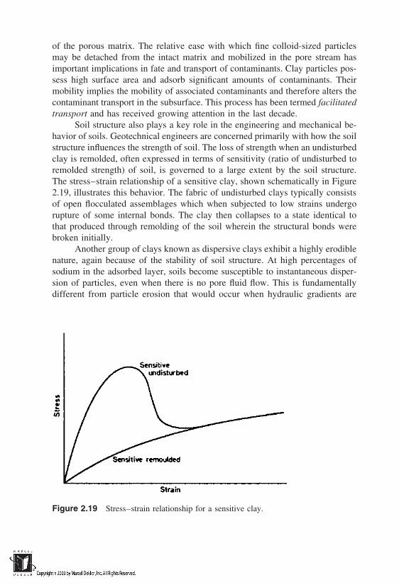
of the porous matrix. The relative ease with which fine colloid-sized particlesmay be detached from the intact matrix and mobilized in the pore stream hasimportant implications in fate and transport of contaminants. Clay particles pos-sess high surface area and adsorb significant amounts of contaminants. Theirmobility implies the mobility of associated contaminants and therefore alters thecontaminant transport in the subsurface. This process has been termed facilitatedtransport and has received growing attention in the last decade.

Soil structure also plays a key role in the engineering and mechanical be-havior of soils. Geotechnical engineers are concerned primarily with how the soilstructure influences the strength of soil. The loss of strength when an undisturbedclay is remolded, often expressed in terms of sensitivity (ratio of undisturbed toremolded strength) of soil, is governed to a large extent by the soil structure.The stress–strain relationship of a sensitive clay, shown schematically in Figure2.19, illustrates this behavior. The fabric of undisturbed clays typically consistsof open flocculated assemblages which when subjected to low strains undergorupture of some internal bonds. The clay then collapses to a state identical tothat produced through remolding of the soil wherein the structural bonds werebroken initially.

Another group of clays known as dispersive clays exhibit a highly erodiblenature, again because of the stability of soil structure. At high percentages ofsodium in the adsorbed layer, soils become susceptible to instantaneous disper-sion of particles, even when there is no pore fluid flow. This is fundamentallydifferent from particle erosion that would occur when hydraulic gradients are

Figure 2.19 Stress–strain relationship for a sensitive clay.

excessive. Two terms, known as sodium adsorption ratio (SAR) and exchange-able sodium percentage (ESP), are used as indicators of dispersive nature ofclays. They are defined as

SAR(mEq/liter)1/2 Na

[(Ca2 Mg2)/2]1/2 (2.32)

ESP (Na)

total exchange capacity(2.33)

The concentrations in the SAR refer to the pore solution, whereas the sodiumconcentration in the ESP refers to the exchange complex of the soil. In general,soils with ESP greater than 2% are considered to be susceptible to dispersion.Sherard et al. (1976) obtained criteria for soil dispersion using a number of experi-mental observations (Fig. 2.20). Three zones were identified: zone A, where dis-persion might be expected; zone B, where dispersion is not likely to occur; andan intermediate zone C, where soils may or may not be dispersive.

A quantitative knowledge of the forces involved in a given structure theo-retically allows one to obtain the strength of soils on a given plane. This, however,requires us to postulate the arrangement of interparticle bonds that lie across theplane. Ingles (1962) attempted to estimate the tensile strength of soils directly,in terms of the microscopic forces of interaction. A consideration of the electro-

Figure 2.20 Influence of total dissolved salts and percent sodium on dispersibility.(Source: Sherard et al., 1976)

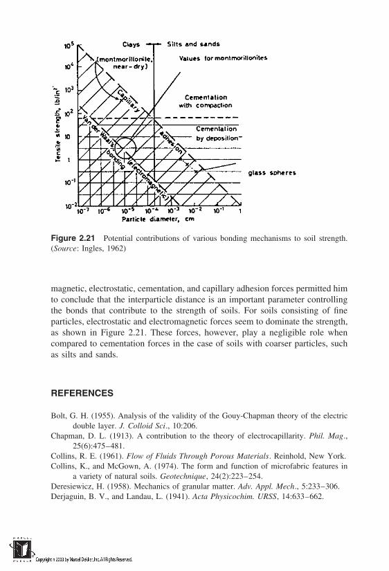
Figure 2.21 Potential contributions of various bonding mechanisms to soil strength.(Source: Ingles, 1962)

magnetic, electrostatic, cementation, and capillary adhesion forces permitted himto conclude that the interparticle distance is an important parameter controllingthe bonds that contribute to the strength of soils. For soils consisting of fineparticles, electrostatic and electromagnetic forces seem to dominate the strength,as shown in Figure 2.21. These forces, however, play a negligible role whencompared to cementation forces in the case of soils with coarser particles, suchas silts and sands.

REFERENCES

Bolt, G. H. (1955). Analysis of the validity of the Gouy-Chapman theory of the electricdouble layer. J. Colloid Sci., 10:206.

Chapman, D. L. (1913). A contribution to the theory of electrocapillarity. Phil. Mag.,25(6):475–481.

Collins, R. E. (1961). Flow of Fluids Through Porous Materials. Reinhold, New York.Collins, K., and McGown, A. (1974). The form and function of microfabric features in

a variety of natural soils. Geotechnique, 24(2):223–254.Deresiewicz, H. (1958). Mechanics of granular matter. Adv. Appl. Mech., 5:233–306.Derjaguin, B. V., and Landau, L. (1941). Acta Physicochim. URSS, 14:633–662.

Dullien, F.A.L. (1992). Porous Media, Fluid Transport and Pore Structure. AcademicPress, London.

Garcia-Bengochea, I., Lovell, C. W., and Altschaeffl, A. G. (1979). Pore distribution andpermeability of silty clays. ASCE J. Geotech. Eng., 105GT7:839–856.

Gouy, G. (1910). Sur la constitution de la charge electrique a la surface d’un electrolyte.Annale Physique (Paris), Ser. 4, 9:457–468.

Griffiths, F. J., and Joshi, R. C. (1989). Change in pore size distribution due to consolida-tion of clays. Geotechnique, 39(1):159–167.

Haughey, D. P., and Beveridge, G. S. G. (1969). Structural properties of packed beds—A review. Can. J. Chem. Eng., 47:130.

Ingles, O. G. (1962). Bonding forces in soils, part 3: A theory of tensile strength forstabilized and naturally coherent soils. Proceedings of the First Conference of theAustralian Road Research Board, Vol. 1, pp. 1025–1047.

Israelachvili, J. (1992). Intermolecular and Surface Forces, 2nd ed. Academic Press, SanDiego.

Lambe, T. W. (1958). Compacted clay: Structure. ASCE J. Soil Mech. Found. Div., Pro-ceedings Paper 1654, pp. 682–706.

Langmuir, I. (1938). Repulsive forces between charged surfaces in water and the causeof the Jones-Ray effect. Science, 88:430.

Mitchell, J. K. (1993). Fundamentals of Soil Behavior, 2nd ed. Wiley, New York.Olsen, H. W. (1962). Hydraulic flow through saturated clay. Proceedings of the Ninth

National Conference on Clays and Clay Minerals, pp. 131–161.Quigley, R. M., and Thompson, C. D. (1966). The fabric of aniostropically consolidated

sensitive marine clay. Can. Geotech. J., 3(2):61–73.Ridgway, K., and Tarbuck, K. J. (1967). Random packing of spheres. Bri. Chem. Eng.,

12(3):384–388.Seed, H. B., and Chan, C. K. (1959). Structure and strength characteristics of compacted

clays. ASCE J. Soil Mech. Found. Div., 85(SM5), Proceedings Paper 2216.Sherard, J. L., Dunnigan, L. P., Decker, R. S., and Steele, E. F. (1976). Identification and

nature of dispersive soils. ASCE J. Geotech. Eng. Div., 102(GT4):187–301.U.S. Department of Agriculture. (1951). Soil Survey Manual, Handbook No. 18.van Olphen, H. (1977). An Introduction to Clay Colloid Chemistry, 2nd ed. Wiley-Intersci-

ence, New York.Verwey, E. J. W., and Overbeek, J. Th. G. (1948). Theory of the Stability of Lyophobic

Colloids. Elsevier, New York.Yong, R. N., and Sheeran, D. E. (1973). Fabric unit interaction and soil behavior Pro-

ccedings of the International Symposium on Soil Structure, Gothenburg, Sweden,pp. 176–183.

3Flow of Water in Soils

3.1 INTRODUCTION

Water is an important phase in soil for a variety of reasons. A study of flow ofwater in soils is essential in diverse disciplines. The energy state of water in soilpores dictates the soil strength, and this is studied in soil mechanics using theeffective stress principle. Soil physics treats the fundamental aspects of theseinteractions as they pertain to agricultural needs, generally dealing with topsoils.Hydrology deals with water quantity and its management, particularly at regionaland global scales. Groundwater flow at aquifer scale is of primary importancein this discipline. In the context of geoenvironmental engineering, we are inter-ested in how the pore water in soils facilitates transport as well as transformationof contaminants. In this chapter, we will study the general principles of porewater flow necessary to understand contaminant transport in soils. While onlywater flow is considered in this chapter, the transport of contaminants in the formof dissolved and immiscible phases associated with this flow will be the centraltheme of Chapters 4 and 5.

The subject of groundwater flow is so broad that it is necessary to divideit into two categories, saturated and unsaturated soils, for the purpose of easierunderstanding. The flow of water is governed by the same driving mechanismsin both cases; however, the presence of air as the third phase requires additionalconsiderations in the case of unsaturated soils. We will first discuss energy statesof water in soils, which provide driving force for flow, before narrowing downto saturated or unsaturated soils. Our objective in this chapter is to lay down thenecessary foundations to address the contaminant transport aspects in Chapters4 and 5.

3.2 ENERGY STATES OF WATER IN SOIL

Water, like any other substance in nature, possesses two types of energy, potentialand kinetic. The potential energy is associated with its position and state withreference to some datum conditions, whereas the kinetic energy is associated withits motion. Fortunately, in most cases, the velocities of water flow in soils arenot significant enough to warrant kinetic energy considerations. To compensatefor this simplicity however, nature has created a variety of sources for soil waterto derive its potential energy from. It is the variation in the total potential energyfrom one location to another that is responsible for water flow in soils. Therefore,it is important for us to understand each of these potential energy sources.

One of the formal definitions for the total potential of soil water, encom-passing all the possible sources, was provided by Aslyng (1963):

[The] amount of work that must be done per unit quantity of pure water inorder to transport reversibly and isothermally an infinitesimal quantity ofwater from a pool of pure water at a specified elevation at atmospheric pres-sure to the soil water (at the point under consideration).

This definition was merely an attempt to view the soil– water potential ina comprehensive manner. It is, of course, practically impossible to evaluate thepotential by transporting water from one point to the other the way it is statedin the definition. Nevertheless, the definition indicates the important factors thatcause variations in potential energy, viz., elevation, pressure, and chemical com-position (indicated by the word, ‘‘pure’’) of water. The definition also uses areference state (‘‘from a pool of pure water at a specified elevation at atmosphericpressure’’) and relates the water potential to that state. By separating the individ-ual contributions, the total potential of soil water, ψ, can be expressed as

ψ ψg ψp ψo (3.1)

where ψg gravitational potential due to difference in elevation alone, ψp pressure potential due to difference in pressure alone, and ψo osmotic potentialdue to differences in chemical composition of water, perhaps due to presence ofsolutes.

The simplest of the three sources is the gravitational potential, ψg, whichis expressed as the product of unit weight of water, γw, and the elevation of thewater body above a specified datum. Thus, the potential energy of a unit volumeof water at a height z1 above a reference elevation is simply

ψg γwz1 (3.2)

As shown in Figure 3.1, ψg is independent of pressure conditions of soil waterand of whether the soil is saturated or unsaturated, and is dependent only on theelevation of water body relative to the datum.

Figure 3.1 Gravitational and pressure potentials.

The pressure potential, ψp, can be positive or negative, depending onwhether the point in soil under consideration is at hydrostatic pressure greaterthan atmospheric pressure, or is at a pressure lower than atmospheric pressure(Fig. 3.1). When it is positive, it implies that the point is below a free watersurface, and is often referred as piezometric or submergence potential. This posi-tive potential can be expressed as

ψp γwz2 (3.3)

where z2 difference in elevation of the point under consideration and watertable, where atmospheric conditions prevail.

When the pressure at the point under consideration is subatmospheric, theenergy required to transport a unit volume of water from atmospheric conditionsis governed by the capillarity principle. The potential in this case is often referredas capillary or matric potential. Water is trapped in the pore space under subatmo-spheric conditions because of the adsorptive forces of the soil matrix. Theseforces are better visualized in terms of the menisci formed when narrow capillarytubes are dipped in a body of free water (Fig. 3.2). The occurrence of meniscusin the capillary tube causes a pressure difference to develop across the interface.If the medium above the water is lighter, such as air, the meniscus is concaveas shown in Figure 3.2; therefore, the pressure under the meniscus is smallerthan the pressure above the meniscus (which is atmospheric in this case). Thispressure difference causes the transport (or rise) of water in the capillary tubefrom the water surface under atmospheric pressure. From the definition of surfacetension, the pressure potential can be expressed as

ψp 2σRm

(3.4)

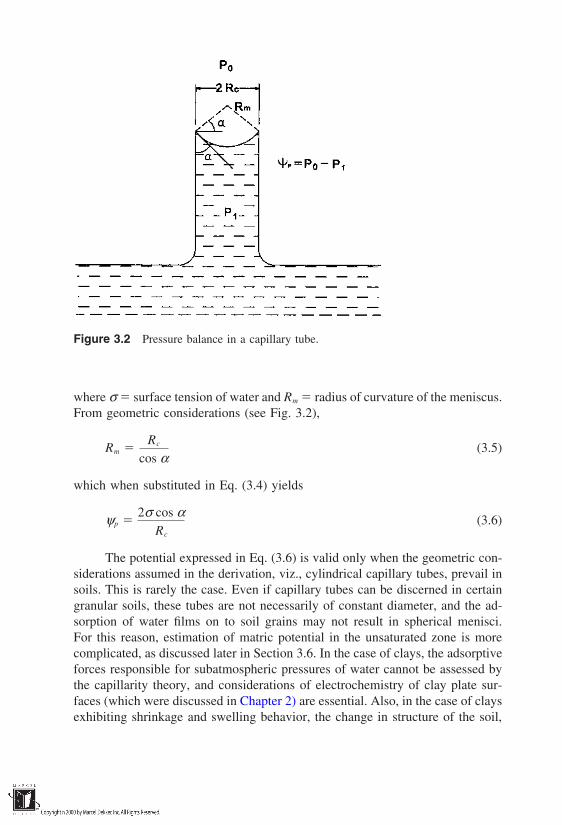
Figure 3.2 Pressure balance in a capillary tube.

where σ surface tension of water and Rm radius of curvature of the meniscus.From geometric considerations (see Fig. 3.2),

Rm Rc

cos α(3.5)

which when substituted in Eq. (3.4) yields

ψp 2σ cos α

Rc

(3.6)

The potential expressed in Eq. (3.6) is valid only when the geometric con-siderations assumed in the derivation, viz., cylindrical capillary tubes, prevail insoils. This is rarely the case. Even if capillary tubes can be discerned in certaingranular soils, these tubes are not necessarily of constant diameter, and the ad-sorption of water films on to soil grains may not result in spherical menisci.For this reason, estimation of matric potential in the unsaturated zone is morecomplicated, as discussed later in Section 3.6. In the case of clays, the adsorptiveforces responsible for subatmospheric pressures of water cannot be assessed bythe capillarity theory, and considerations of electrochemistry of clay plate sur-faces (which were discussed in Chapter 2) are essential. Also, in the case of claysexhibiting shrinkage and swelling behavior, the change in structure of the soil,

coupled with the mechanical forces exerted by the matrix on the pore water, makeit difficult to assess the matric potential.

In spite of the limitations, the capillarity principle allows us to understandthe factors that cause negative potential, and its usefulness goes beyond the mereexpression of matric potential. In cases where soil pores are occupied by immisci-ble fluids other than air, such as gasoline (popularly termed NAPLs for Non-Aqueous-Phase Liquids), the principle allows us to characterize the entrapmentof the fluid. These issues will be dealt with in Chapter 5.

In dealing with the pressure potentials, it is important to account for theambient pressure changes in the air. When the air pressure at the reference (atmo-spheric) state is different from the air pressure in soil at the point under consider-ation, the difference in the pressure (termed pneumatic potential) must be addedto either the positive or the negative pressure potential.

The differences in osmotic potential of soil water, ψo, are due to the changesin chemical composition. The presence of solutes in the soil water lowers thevapor pressure and reduces the potential energy of water to a small extent. Thisis traditionally explained using the semipermeable membrane concept. When amembrane permeable only to water and not to the solute separates the soil solu-tion and pure water, a process called osmosis causes the water to diffuse into thesolution side in an attempt to equilibrate the solute concentrations. The hydro-static pressure that exists across the barrier as a result of this diffusion processcauses osmotic potential. Although this potential is relatively small when com-pared to the others described above, it is of importance when we consider thechemical transport across barriers in vapor phase. The magnitude of the osmoticpotential is dependent on the concentration of the solute and its temperature. Fordilute solutions, it can be approximated by (Slatyer, 1967)

ψo MCT (3.7)

where M molar concentration of the solute particles, C universal gas constant(8.32 107 erg/mol deg), and T absolute temperature.

Let us carry the membrane concept further to understand the combinedeffect of matric potential and osmotic potential. This is best illustrated in Figure3.3. Notice that the gravitational potential does not exist because of the fact thatthe elevations of both reference solution (pure water) and the soil solution arethe same. The membrane to the immediate left of the soil sample separates thefree soil solution with soil sample and therefore is subjected to a pressure differ-ence due to capillary potential alone. The second membrane to the far left of thesample separates pure water and soil solution and is therefore subjected to os-motic potential alone. The combined effect of the two potentials is shown by thesingle membrane on the right of the sample, which separates the subatmosphericsoil solution in the soil and pure water.

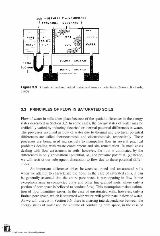
Figure 3.3 Combined and individual matric and osmotic potentials. (Source: Richards,1965)

3.3 PRINCIPLES OF FLOW IN SATURATED SOILS

Flow of water in soils takes place because of the spatial differences in the energystates described in Section 3.2. In some cases, the energy states of water may beartificially varied by inducing electrical or thermal potential differences in water.The processes involved in flow of water due to thermal and electrical potentialdifferences are called thermoosmosis and electroosmosis, respectively. Theseprocesses are being used increasingly to manipulate flow in several practicalproblems dealing with waste containment and site remediation. In most casesdealing with flow assessment in soils, however, the flow is dominated by thedifferences in only gravitational potential, ψg, and pressure potential, ψp; hence,we will restrict our subsequent discussion to flow due to these potential differ-ences.

An important difference arises between saturated and unsaturated soilswhen we attempt to characterize the flow. In the case of saturated soils, it canbe generally assumed that the entire pore space is participating in flow (someexceptions arise in compacted clays and other fine-grained soils, where only aportion of pore space is believed to conduct flow). This assumption makes estima-tion of flow quantities easier. In the case of unsaturated soils, however, only alimited pore space, which is saturated with water, will participate in flow of water.As we will discuss in Section 3.6, there is a strong interdependence between theenergy states of water and the volume of conducting pore space, in the case of

unsaturated soils. This complication makes it necessary and convenient to treatthe saturated and unsaturated flow separately.

Earlier attempts to conceptualize flow in soils assumed that the soil massis analogous to a bundle of parallel capillary tubes, which are not connected toeach other. This assumption enabled application of our knowledge of hydraulicsin pipes to characterize flow. We will start with the principles of flow in a singlecapillary tube (using Poiseuille’s law) and work our way up to extrapolating theseprinciples to soils (using Darcy’s law). This treatment will give us valuable in-sight into one of the most important properties of soils—the coefficient of perme-ability—and some methods to evaluate this property.

3.3.1 Poiseuille’s and Darcy’s Laws

We will first consider flow through a single capillary tube (Fig. 3.4) due to differ-ence in pressure potential, ∆P. This potential difference between the two endsof the tube is the driving force for flow, which takes place against the frictionalresistance offered by the viscosity of water. The force F acting on an annularcylinder of water of radius r due to pressure difference ∆P is

F ∆P(πr2) (3.8)

This force is resisted by the shear stress τ at the interface between the annularring and the rest of the water body. Equating the two forces for equilibrium,

F ∆P(πr2) τ (2πrL) (3.9)

Figure 3.4 Flow through a single capillary tube.

which yields an expression for the shear stress in terms of the potential difference:

τ (∆P)r

2L(3.10)

The fundamental law of viscosity given by Newton gives us another expressionfor the shear stress τ in terms of the radius-dependent velocity of flow Vt(r) inthe tube,

τ η dVt(r)dr

(3.11)

where η viscosity of water. Combining Eqs. (3.10) and (3.11) and integratingwithin the limits of r and R will yield

Vt(r) ∆P

4Lη(R2 r2) (3.12)

In obtaining Eq. (3.12), we used a no-slip boundary condition, which means thatat the walls of the tube (r R), Vt 0. Equation (3.12) indicates that the changein velocity with respect to the radius is parabolic in nature. To calculate the waterdischarge, i.e., the amount of flow per unit time (qt) Eq. (3.12) must be integratedacross the cross-sectional area of the tube. This amounts to the volume of a para-boloid of revolution. Leaving the integration exercise to the reader, we expressthe end result as

qt πR2

2 ∆PR2

4Lη πR4

8η ∆P

L (3.13)

This is an important equation known as Poiseuille’s law. It shows that the dis-charge through a capillary tube is directly proportional to the difference in pres-sure potential ∆P across the length of the tube, and to the fourth power of theradius of the tube, R. Equation (3.13) can be rewritten in terms of the area ofcross-section of the tube At as

qt R2

8η ∆P

L (At) where At πR2 (3.14)

which in turn enables us to express the ‘‘average’’ velocity of flow Vt in thecapillary tube as

Vt qt

At

R2

8η ∆P

L (3.15)

The first term on the right-hand side of Eq. (3.15) can now be treated as a constant,expressing the proportionality between flow velocity and the pressure gradientin the capillary tube, ∆P/L.

The flow considerations in a single capillary tube described above makeus speculate that when we idealize a soil system as a bundle of parallel capillarytubes, the flow velocities in soils may also exhibit proportionality with respectto the difference in pressure gradient. This was indeed found to be true experi-mentally by Henry Darcy in 1856. A direct proportionality between the flow rateand the pressure potential difference was observed by him. Expressed mathemati-cally,

q k∆P

L A (3.16)

where q is the discharge through the soil sample, A is the area of cross sectionof the sample, and k is a constant of proportionality. Equation (3.16) is one ofthe most commonly used expressions of Darcy’s law for characterization of flowin soils.

The validity of Darcy’s law for soil systems was studied in a number ofinvestigations subsequent to that of Darcy. There were some investigations sug-gesting that the linearity between flow rate and the hydraulic gradient may notbe obeyed at very low or at very high gradients. Equation (3.16) suggests thatthe relationship between q and gradient (∆P/L) is linear. At low hydraulic gradi-ents, a threshold gradient was noticed in some studies below which flow did nottake place in fine-grained soils (Swartzendruber, 1962). Similarly, at high hydrau-lic gradients corresponding to Reynolds number greater than 10, flow in soilsmay not obey Darcy’s law (Bear, 1972). Fortunately, in a majority of cases ofimportance in groundwater flow, these conditions do not occur. When the condi-tions are such that the fluid can be categorized as Newtonian (obeying Newton’slaw of friction) and the flow conditions are in the laminar flow range, Darcy’slaw is in general believed to be applicable to soil systems.

3.3.2 Coefficient of Permeability

A comparison of Eqs. (3.14) and (3.16) indicates that the proportionality constantk encompasses the effects of both soil structure (represented by the pore radii) andthe viscous property of the liquid on flow rates. The constant of proportionality isknown as the coefficient of permeability, and is one of the most researched prop-erties of soils. It exhibits the widest range of variability among all engineeringproperties of soils, with its value ranging from 102 cm/sec in gravels to 1010

cm/sec in clays. Considering that the discharge q is a product of flow velocityand area of cross section,

q VA (3.17)

the velocity of flow in soils, V, can be expressed as

V k∆P

L (3.18)

We should note that the velocity given by Eq. (3.18) is only superficial,since the gross area A was used to express the discharge q in Eq. (3.17) althoughonly the porous area of the cross section contributes to flow. Recognizing thatporosity n could be used to relate total and pore areas in a given cross section,the actual pore velocity, Va may be expressed as

Va V

n(3.19)

This distinction between superficial and actual velocities is important inour discussion of contaminant transport later on. Common ways of obtainingpermeability coefficient typically involve observing the discharge through thesoil system under an applied pressure gradient ∆P/L, and using Eq. (3.16). Assuch, these methods are only indirect. A direct approach to determining perme-ability coefficient requires a thorough characterization of the pore geometry. Ko-zeny (1927) and Carman (1956) provided one of the earliest approaches to linkpermeability of granular soils with their pore geometry. This approach is basedon a more rational extrapolation of Poiseuille’s law of flow through capillarytubes to soil systems with irregular pore space. It provides a useful link betweenthe coefficient of permeability and the void ratio, which is a macroscopic indica-tor of the pore space. For this reason, we will briefly discuss below the Kozeny-Carman equation.

We start with flow in a single capillary tube [Eq. (3.14)] and, in anticipationof having to deal with irregular cross sections, we express the size of the poretube in terms of the hydraulic radius, RH. Using RH allows us to generalize theexpression for any shape of the tube, and it will eventually yield an expressionin terms of void ratio, e. Therefore, for a capillary tube of any geometric shape,flow can be expressed as

qt CsR2

H

ηia (3.20)

where i pressure gradient ∆P/L, a area of cross section of the irregularpore tube, and Cs shape constant. We now apply Eq. (3.20) to a soil sampleand attempt to express a and RH in terms of measurable parameters. The area of

an irregular cross section, a, can be written in terms of the total cross-sectionalarea, A, as

a nA (3.21)

where n porosity of the soil sample. RH, on the other hand, may be expressedas

RH flow area

wetted perimeter

flow volumewetted area

eVs

VsSo

e

So

(3.22)

where Vs volume of solid particles in the sample, and So wetted surfacearea per unit volume of solid particles. Note that the entire pore volume of soilis assumed to participate in flow in Eq. (3.22). Substitution of Eqs. (3.21) and(3.22) in Eq. (3.20) with the equality n e/(1 e) yields

q Cs 1ηS2

o e3

1 eiA (3.23)

By analogy of Eq. (3.23) with Darcy’s law [Eq. (3.16)], permeability coef-ficient k may be expressed as

k Cs 1ηS2

o e3

1 e (3.24)

Equation (3.24) gives us a valuable relationship between k and e; however,its use is possible only when we can quantify the two constants, Cs and So, whichare difficult to estimate. This is primarily the reason why this equation has re-mained academic, with little potential for practical application. The proportional-ity between k and e is, however, a useful result, which led Casagrande to proposea simple and practical expression for k of sands as a function of e:

k(e) 1.4k0.85e2 (3.25)

where k0.85 permeability at a void ratio of 0.85. In the case of coarse-grainedsoils such as sands, void ratio is dependent on the representative size of soilgrains. This led to another useful expression between permeability and the effec-tive size of soils (Hazen, 1911):

k(cm/s) CD210 (3.26)

where D10 effective size in centimeter and C a proportionality constantvarying from 90 to 120. Although the proportionality between k and void ratioor effective size of grains is usually obeyed in the case of coarse-grained soilssuch as sands and silts, serious discrepancies are observed when such equationsare applied to clays. Because of the additional and more dominant factors influ-

encing the soil structure, such equations are of limited use in compacted clays,as seen in the next section.

Permeability coefficient k is a lumped parameter encompassing the fluidproperties (primarily the viscosity) and the pore space geometry of the media. Itis convenient to separate the effects of the fluid and the media parameters. Forinstance, one may be interested in the effects of pore space geometry alone onpermeability of a given fluid. A property defined as ‘‘intrinsic’’ or ‘‘absolute’’permeability is often used to address permeability in terms of only media proper-ties. Excluding the viscosity of pore fluid from Eq. (3.24), the intrinsic permeabil-ity may be expressed as

ka Cs

S2o e3

1 e (3.27)

Equation (3.27) contains only soil parameters, and a comparison with Eq. (3.24)indicates that

k ka

η(3.28)

While the term ‘‘coefficient of permeability’’ refers to the permeation of anyfluid in general, the term ‘‘hydraulic conductivity’’ is used specifically to denotethe permeability of water. This distinction, however, is not followed strictly in theliterature. Of the two sets of properties—those of the fluid and the media—the effect of the former on k is easier to evaluate. k is inversely proportionalto the viscosity, η [Eq. (3.28)]. For a given fluid, the variation of viscosity withrespect to temperature is well known, and therefore permeability values obtainedat a given temperature may be translated to those at any other temperature usingthis variation. When reporting the permeability, it is customary to standardizethe values at 20°C (70°F), and have the user transform the standardized perme-ability to a specific temperature using the relation

k20

kt

ηt

η20

(3.29)

where the subscript denotes the temperature in degrees celsius.The effect of pore space geometry on k is not easy to evaluate, since it is

a consequence of a number of variables, viz., grain size distribution, density, andstructure of the soil. Soil systems with smaller particle sizes are naturally ex-pected to be associated with smaller pore openings and are likely to exhibit lowerpermeability. Similarly, an increase in density of the soil, either by compactionor consolidation, will reduce the size of the pore openings and therefore willresult in a smaller k. Figure 3.5 shows the effects of particle size and soil densityon coefficient of permeability. It is important to notice the wide range of variabil-

ity in k, 101 to 1010 cm/s, which is perhaps greater than variability in any otherengineering parameter of soils.

Prediction of the influence of soil structure on permeability is perhaps oneof the greatest challenges that has not yet been met. This is especially true in thecase of compacted clays. The soil structure, discussed in Chapter 2, is governednot only by the physicochemical properties of soils, but also by the mode ofpreparation in the case of compacted clays. It is possible to compact two soilssuch that they both have the same void ratio but differ greatly in their fabric andstructure. Considering the importance of compacted clays in waste-containmentstructures dealt with later in this book, it is appropriate to take up this topic atsome length.

3.3.3 Permeability of Compacted Clays

The preparation of compacted clays involves choice of molding water content,energy of compaction, and type of compaction—all of which together governtheir dry density. A number of studies conducted over the past few decades indi-cate that the void ratio of compacted clays [which is uniquely related to drydensity, see Eq. (1.14)] is not the only factor governing the permeability. Thisis attributed mainly to the microstructure, which is not unique for a given voidratio. It is difficult to characterize quantitatively the particle orientation and theresulting pore structure in compacted clays from qualitative information such asthat shown in Figure 2.17. This makes it difficult to develop a theoretical basisfor prediction or estimation of permeability of compacted clays in terms of thechanges in soil structure.

The complexity of permeability behavior of compacted clays is best illus-trated in Figure 3.6. We see that permeability varies by several orders magnitudealthough the four clays were prepared at nearly the same conditions of moldingwater content and maximum dry density. This is typical of compacted clays, andattempts to develop mathematical expressions for permeability have not beencompletely successful. Research during the last two decades, done in the contextof waste containment, however, has resulted in useful information on the impor-tant variables affecting permeability of compacted clays. In general, the parame-ters responsible for such wide variation of permeability in the case of compactedclays can be grouped into three categories:

1. Variables involved in the preparation of compacted clays2. Chemistry of the permeant3. Testing methods

The effect of compaction variables on the microstructure and k of com-pacted clays was first studied by Mitchell et al. (1965) and is shown in Figure 3.7.This figure shows that, in general, reduction of two to three orders of magnitude in

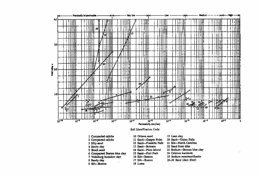
Figure 3.6 Variability in coefficient of permeability of compacted clays.

Figure 3.5 Laboratory results showing the effect of soil type (indicative of particle size)and void ratio (indicative of soil density) on coefficient of permeability. (Source: Lambeand Whitman, 1969)

Figure 3.7 Variation of coefficient of permeability with respect to molding water con-tent and compaction effort. (Source: Mitchell et al. 1965)

permeability may result as the structure of clay changes from dry-of-optimumto wet-of-optimum. The lowest permeability occurs wet-of-optimum, beyondwhich a slight rebound is possible. This is the basis for the current practice ofpreparing compacted clays wet-of-optimum in the construction of clay liners forwaste containment. The permeabilities in Figure 3.7 correspond to saturated statewith saturation achieved from the initial molding state. A replot of the same datain Figure 3.8 brings out the sharp contrast between sands and compacted claysin that the permeability of compacted clays does not depend uniquely on the drydensity (or void ratio). For the molding water content of 19%, the permeabilitychanged almost three orders of magnitude, although the dry density is constant.More recent studies established the effects of such variables as type and energyof compaction and size of clods used in the compaction process. Field compactionof soils can be done using different methods, including impact, static, kneading,and vibratory methods. The compaction method adopted greatly influences the

Figure 3.8 Inadequacy of dry density (which is indicative of void ratio) as a macro-scopic indicator of permeability in the case of compacted clays. (Source: Mitchell et al.1965)

fabric and hence the permeability of compacted clay. For a detailed descriptionof these issues, the reader is referred to Day and Daniel (1985) and Daniel (1987).The effect of clod sizes on permeability could be understood in terms of Olsen’scluster model (Fig. 2.5). Reduction of clod sizes and elimination of interclodpores would result in smaller minifabric pores, which would in turn result inlower permeability. This has been established experimentally by Benson andDaniel (1990).

Unlike the case of sands, the chemistry of the permeant (in addition to thephysical property of viscosity) influences the permeability of compacted clays.This is because of the surface chemistry which clay particles exhibit when inter-acting with the pore fluid during the molding stages as well as during the perme-ation stages. The diffuse double-layer theory discussed in Chapter 2 provides abasis on which to draw general conclusions on how the permeant chemistry altersthe microstructure of compacted clays. Based on whether the permeant is promot-

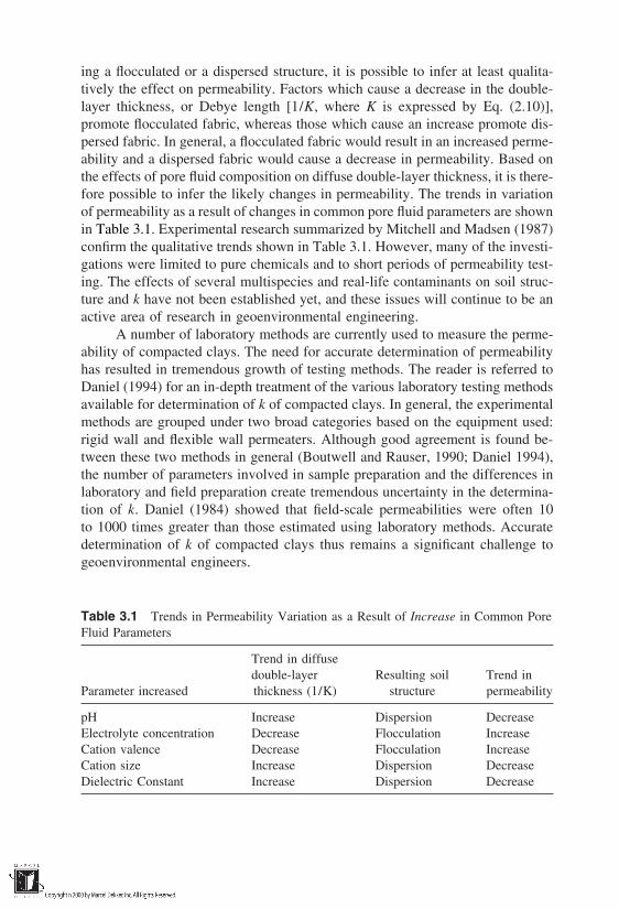
ing a flocculated or a dispersed structure, it is possible to infer at least qualita-tively the effect on permeability. Factors which cause a decrease in the double-layer thickness, or Debye length [1/K, where K is expressed by Eq. (2.10)],promote flocculated fabric, whereas those which cause an increase promote dis-persed fabric. In general, a flocculated fabric would result in an increased perme-ability and a dispersed fabric would cause a decrease in permeability. Based onthe effects of pore fluid composition on diffuse double-layer thickness, it is there-fore possible to infer the likely changes in permeability. The trends in variationof permeability as a result of changes in common pore fluid parameters are shownin Table 3.1. Experimental research summarized by Mitchell and Madsen (1987)confirm the qualitative trends shown in Table 3.1. However, many of the investi-gations were limited to pure chemicals and to short periods of permeability test-ing. The effects of several multispecies and real-life contaminants on soil struc-ture and k have not been established yet, and these issues will continue to be anactive area of research in geoenvironmental engineering.

A number of laboratory methods are currently used to measure the perme-ability of compacted clays. The need for accurate determination of permeabilityhas resulted in tremendous growth of testing methods. The reader is referred toDaniel (1994) for an in-depth treatment of the various laboratory testing methodsavailable for determination of k of compacted clays. In general, the experimentalmethods are grouped under two broad categories based on the equipment used:rigid wall and flexible wall permeaters. Although good agreement is found be-tween these two methods in general (Boutwell and Rauser, 1990; Daniel 1994),the number of parameters involved in sample preparation and the differences inlaboratory and field preparation create tremendous uncertainty in the determina-tion of k. Daniel (1984) showed that field-scale permeabilities were often 10to 1000 times greater than those estimated using laboratory methods. Accuratedetermination of k of compacted clays thus remains a significant challenge togeoenvironmental engineers.

Table 3.1 Trends in Permeability Variation as a Result of Increase in Common PoreFluid Parameters

Trend in diffusedouble-layer Resulting soil Trend in

Parameter increased thickness (1/K) structure permeability

pH Increase Dispersion DecreaseElectrolyte concentration Decrease Flocculation IncreaseCation valence Decrease Flocculation IncreaseCation size Increase Dispersion DecreaseDielectric Constant Increase Dispersion Decrease

3.4 GOVERNING EQUATION FOR SATURATED FLOW

We now proceed to use Darcy’s law and the permeability concept to develop amathematical equation governing the saturated flow process. We seek a generalexpression that controls the process in a flow domain of any given shape andunder any given set of initial and boundary conditions. As we do with similarprocesses, we invoke the universal law of mass conservation and couple it witha cause-and-effect relationship, which in this case is Darcy’s law. The readermay observe parallelism between this and other processes in solid mechanics(where force equilibrium is coupled with Hooke’s law), in heat conduction (whereenergy conservation is coupled with the law of thermal conductivity), etc.

We apply mass conservation principle to an elemental control volumeshown in Figure 3.9. With reference to this volume, the principle dictates:

(Rate of mass output) (rate of mass input) (rate of change in storage in the elemental control volume)

(3.30)

When expressed mathematically in all three dimensions, the left-hand side of Eq.(3.30) becomes

ρVx ∂

∂x(ρVx) ρVx ρVy

∂∂y

(ρVy) ρVy ρVz ∂∂z

(ρVz) ρVz

Figure 3.9 Mass conservation in an elemental control volume.

or

∂∂x

(ρVx) ∂∂y

(ρVy) ∂∂z

(ρVz)

where ρ density of the liquid, and Vx, Vy, and Vz velocities of flow in thex, y, and z dimensions.

Storage in the elemental control volume changes due to either a change indensity of the fluid, which causes expansion or contraction of the fluid, or achange in pore volume of the element. The latter is in turn due to time-dependentcompressibility of the soil. For fine-grained soils, this is well known to geotechni-cal engineers as consolidation process. Accounting for these two factors on theright-hand-side of Eq. (3.30), the mass conservation principle may be expressedas

∂∂x

(ρVx) ∂

∂y(ρVy)

∂∂z

(ρVz) ∂∂ t

(ρn) (3.31)

Rate of change in storage is usually expressed in terms of a parameter knownas specific storage, Ss, which is defined as the volume of water that a unit volumeof aquifer releases from storage under a unit decline in hydraulic head. Thisparameter can be expressed to include the effects of compressibility of the fluidand the medium as (see Freeze and Cherry, 1979)

Ss ρg(α nβ ) (3.32)

where α compressibility of the pore medium defined as the change in the bulksoil volume per unit change in effective stress, and β compressibility of thefluid defined as the change in its volume per unit change in pore water pressure,u. Thus,

α dVT/VT

dσ(3.33)

and

β dVw/Vw

du(3.34)

As will be seen later, Eq. (3.33) provides a link between saturated flow equationand Terzaghi’s consolidation equation.

Expressed in terms of specific storage, the mass conservation principle [Eq.(3.31)] can be rewritten as

∂∂x

(ρVx) ∂∂y

(ρVy ∂∂z

(ρVz) ρSs∂h

∂ t(3.35)

where h hydraulic head. We now incorporate Darcy’s law to write velocitycomponents with pressure potentials expressed in terms of hydraulic head, h:

∂∂xkx

∂h

∂x ∂∂yky

∂h

∂y ∂∂zkz

∂h

∂z Ss∂h

∂t(3.36)

where kx, ky, and kz are permeabilities in the x, y, and z dimensions, respectively,ρ is eliminated in Eq. (3.36) because the variation of velocity components is muchgreater than that of ρ with respect to space coordinates. This would eliminatethe Vx(∂ρ/∂x), Vy(∂ρ/∂y), and Vz(∂ρ/∂z) components when the left-hand side isexpanded using the chain rule. Assuming that the saturated medium is homoge-neous and isotropic (kx ky kz k), Eq. (3.36) can be simplified as

∂ 2h

∂x2

∂ 2h

∂y2

∂ 2h

∂z2

Ss

k

∂h

∂ t(3.37)

Most groundwater-flow modeling activities involve solving Eq. (3.37) inone form or other for a specific domain of interest. While closed-form solutionsexist for certain special cases, numerical methods are in general necessary. Wewill discuss below a few special cases to gain insight into saturated flow prob-lems.

3.5 SPECIAL CASES OF SATURATED FLOW

3.5.1 Steady-State Saturated Flow: Flow Nets

Under steady-state conditions, when there is no change in storage of the porousmedia, Eq. (3.37) reduces to the well-known Laplace equation:

∂ 2h

∂x2

∂ 2h

∂y2

∂ 2h

∂z2 ∇ 2h 0 (3.38)

Starting with the simplest situation of one-dimensional flow, such as the case ina thin laboratory soil column (Fig. 3.10),

∂ 2h

∂x2 0 (3.39)

Integration of Eq. (3.39) twice gives us the general solution,

h C1x C2 (3.40)

where C1 and C2 are integration constants. To evaluate these constants, we usethe following simple boundary conditions:

h h1 at x 0 (3.41)

Figure 3.10 One-dimensional steady-state saturated flow.

and

h h2 at x L (3.42)

where h1 h2. For these conditions, the solution becomes

h h1 (h1 h2)x

L(3.43)

which simply states an intuitive fact—that the pressure potential is dissipatedlinearly with respect to the length of travel (see Fig. 3.10).

For two-dimensional flow, Eq. (3.38) becomes

∂ 2h

∂x2

∂ 2h

∂y2 0 (3.44)

For this situation, one can show that there exist two mathematical functions, φ(x,y) and ψ(x, y), such that

∂φ∂x

k∂h

∂x(3.45)

∂ψ∂x

k∂h

∂y(3.46)

∂φ∂y

k∂h

∂y(3.47)

and

∂ψ∂y

k∂h

∂x(3.48)

which satisfy the governing Eq. (3.44). To understand the usefulness of thesearbitrary functions, φ(x, y) and ψ(x, y), let us consider Eq. (3.45). Integration ofboth sides of Eq. (3.45) with respect to x yields

φ(x, y) kh(x, y) C3 (3.49)

or

h(x, y) 1k

[C3 φ(x, y)] (3.50)

where C3 is a constant of integration. A constant pressure potential h(x, y) indi-cates that φ(x, y) constant. Thus, the curve represented by φ(x, y) constantwould correspond to a constant pressure potential. Such a curve is called anequipotential line. A number of equipotential lines can be drawn in a flow fieldby using different constants for h (x, y). Similarly, ψ(x, y) constant representsanother set of curves on the (x, y) plane. These are called flow lines, because theslope of these curves in the (x, y) plane is in the same direction as the resultantvelocity. This follows from a simple chain-rule differentiation of ψ(x, y) con-stant:

dy

dxψ

Vy

Vx

(3.51)

Similarly, we can show, by differentiating φ(x, y) constant, that

dy

dxφ

Vx

Vy

(3.52)

From Eqs. (3.51) and (3.52), we note that φ(x, y) and ψ(x, y) yield mutuallyperpendicular sets of curves. This mathematical outcome gave us the powerfultechnique to solve saturated flow problems using the graphical method of drawingflow nets. It is a simple technique, which involves drawing two sets of linesperpendicular to each other in the flow domain consistent with boundary condi-tions. The flow net offers a useful method to estimate pressure potentials in aflow domain and also to estimate the seepage quantities. We demonstrate this

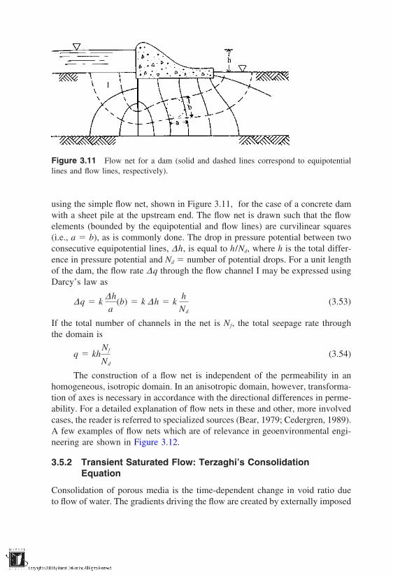
Figure 3.11 Flow net for a dam (solid and dashed lines correspond to equipotentiallines and flow lines, respectively).

using the simple flow net, shown in Figure 3.11, for the case of a concrete damwith a sheet pile at the upstream end. The flow net is drawn such that the flowelements (bounded by the equipotential and flow lines) are curvilinear squares(i.e., a b), as is commonly done. The drop in pressure potential between twoconsecutive equipotential lines, ∆h, is equal to h/Nd, where h is the total differ-ence in pressure potential and Nd number of potential drops. For a unit lengthof the dam, the flow rate ∆q through the flow channel I may be expressed usingDarcy’s law as

∆q k∆h

a(b) k ∆h k

h

Nd

(3.53)

If the total number of channels in the net is Nf, the total seepage rate throughthe domain is

q khNf

Nd

(3.54)

The construction of a flow net is independent of the permeability in anhomogeneous, isotropic domain. In an anisotropic domain, however, transforma-tion of axes is necessary in accordance with the directional differences in perme-ability. For a detailed explanation of flow nets in these and other, more involvedcases, the reader is referred to specialized sources (Bear, 1979; Cedergren, 1989).A few examples of flow nets which are of relevance in geoenvironmental engi-neering are shown in Figure 3.12.

3.5.2 Transient Saturated Flow: Terzaghi’s ConsolidationEquation

Consolidation of porous media is the time-dependent change in void ratio dueto flow of water. The gradients driving the flow are created by externally imposed

Figure 3.12 Examples of flow nets in groundwater flow problems: (a) flow toward awell in a phreatic aquifer; (b) flow in an aquifer with an infinite array of wells; (c) a regionof uniform flow with a pair of pumping and recharge wells. (Source: Bear, 1979)

pressures in excess of existing hydrostatic pressures. The time dependence is dueto the gradual transfer of excess pressure from pore water to solid grains. Since itinvolves flow with simultaneous change in storage (void ratio), the consolidationprocess can be treated as a special case of saturated flow. Using Eq. (3.32) forSs, in Eq. (3.37), the saturated flow for a compressible soil structure can be ex-pressed as

∂ 2h

∂x2

∂ 2h

∂y2

∂ 2h

∂z2

ρgαk

∂h

∂ t(3.55)

Note that we assumed the fluid to be incompressible (i.e., β 0). The com-pressibility of the medium α was defined earlier [see Eq. (3.33)]. The change inbulk volume VT can be taken to be equal to the change in pore volume, since itis reasonable to assume that the solid particles are incompressible. α may there-fore be expressed as

α dVv /VT

dσ

de

(1 e0) dσ(3.56)

where e0 initial void ratio of the medium. The change in void ratio per unitchange in effective stress is typically obtained in the laboratory by conductingconsolidation experiments on soil samples. This is the slope of the e versus σcurve, av, shown in Figure 3.13.

Figure 3.13 Schematic variation of void ratio with respect to effective stress.

Considering a one-dimensional consolidation process in the vertical dimen-sion z, Eq. (3.55) may now be expressed as

∂ 2h

∂z2

av

1 e0ρg

k ∂h

∂ t(3.57)

We recognize here that the total hydraulic head can be divided into two compo-nents, hydrostatic head and head due to excess pore pressures. Therefore,

h h0 u

γw

(3.58)

where h0 hydrostatic head and u excess pore pressure. Limiting ourselvesto problems where h0 is constant,

∂ 2h

∂ z2

1γw

∂ 2u

∂z2(3.59)

and

∂h

∂ t

1γw

∂u

∂ t(3.60)

Substituting Eqs. (3.59) and (3.60) in Eq. (3.57),

1γw

∂ 2u

∂z2

av

(1 e0)k

∂u

∂ t(3.61)

or, in its most familiar form,

∂u

∂ t Cv

∂ 2u

∂z2(3.62)

where Cv is known as the coefficient of consolidation and is given by

Cvk(1 e0)

avγw

(3.63)

Equation (3.62) is the consolidation equation originally studied by Karl Terzaghi(1925). It is similar in form to the heat conduction equation, and a closed-formsolution is possible using Laplace transforms for simple initial and boundary

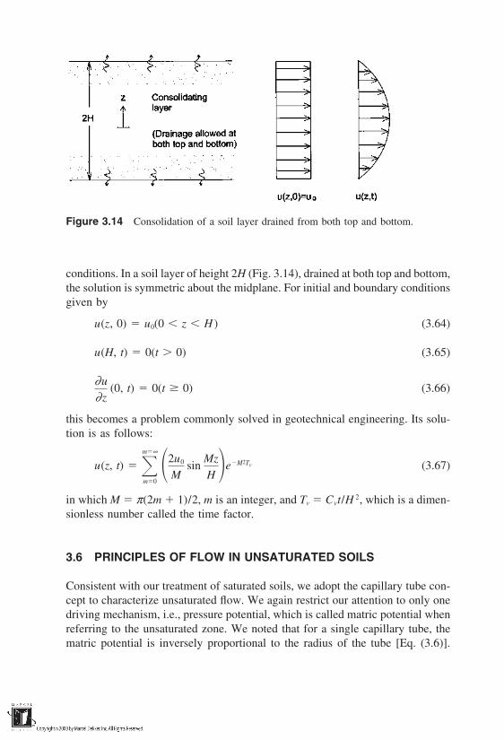
Figure 3.14 Consolidation of a soil layer drained from both top and bottom.

conditions. In a soil layer of height 2H (Fig. 3.14), drained at both top and bottom,the solution is symmetric about the midplane. For initial and boundary conditionsgiven by

u(z, 0) u0(0 z H ) (3.64)

u(H, t) 0(t 0) (3.65)

∂u

∂z(0, t) 0(t 0) (3.66)

this becomes a problem commonly solved in geotechnical engineering. Its solu-tion is as follows:

u(z, t) m∞

m02u0

Msin

Mz

H eM2Tv (3.67)

in which M π(2m 1)/2, m is an integer, and Tv Cvt/H 2, which is a dimen-sionless number called the time factor.

3.6 PRINCIPLES OF FLOW IN UNSATURATED SOILS

Consistent with our treatment of saturated soils, we adopt the capillary tube con-cept to characterize unsaturated flow. We again restrict our attention to only onedriving mechanism, i.e., pressure potential, which is called matric potential whenreferring to the unsaturated zone. We noted that for a single capillary tube, thematric potential is inversely proportional to the radius of the tube [Eq. (3.6)].

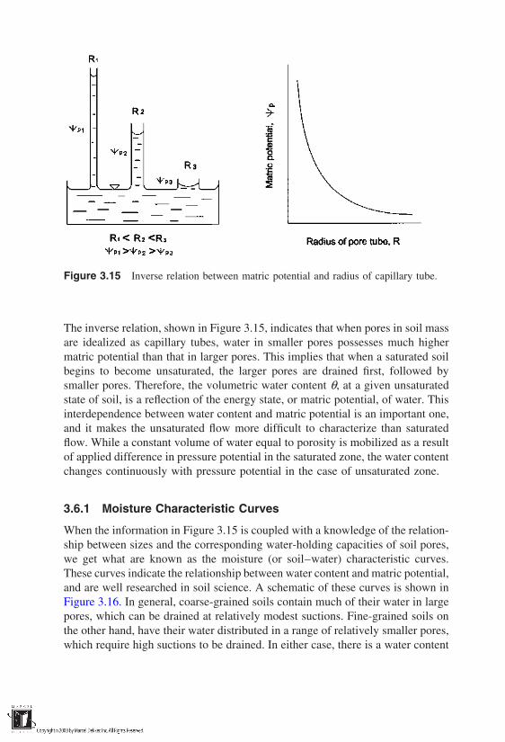
Figure 3.15 Inverse relation between matric potential and radius of capillary tube.

The inverse relation, shown in Figure 3.15, indicates that when pores in soil massare idealized as capillary tubes, water in smaller pores possesses much highermatric potential than that in larger pores. This implies that when a saturated soilbegins to become unsaturated, the larger pores are drained first, followed bysmaller pores. Therefore, the volumetric water content θ, at a given unsaturatedstate of soil, is a reflection of the energy state, or matric potential, of water. Thisinterdependence between water content and matric potential is an important one,and it makes the unsaturated flow more difficult to characterize than saturatedflow. While a constant volume of water equal to porosity is mobilized as a resultof applied difference in pressure potential in the saturated zone, the water contentchanges continuously with pressure potential in the case of unsaturated zone.

3.6.1 Moisture Characteristic Curves

When the information in Figure 3.15 is coupled with a knowledge of the relation-ship between sizes and the corresponding water-holding capacities of soil pores,we get what are known as the moisture (or soil–water) characteristic curves.These curves indicate the relationship between water content and matric potential,and are well researched in soil science. A schematic of these curves is shown inFigure 3.16. In general, coarse-grained soils contain much of their water in largepores, which can be drained at relatively modest suctions. Fine-grained soils onthe other hand, have their water distributed in a range of relatively smaller pores,which require high suctions to be drained. In either case, there is a water content

Figure 3.16 Schematic of moisture characteristic curves.

(known as irreducible or residual water content) below which water cannot bepractically drained, and the moisture characteristic curve goes asymptotic to thematric potential axis. A number of relationships have been suggested in the soilscience literature for moisture characteristic curves. The expressions commonlyused are listed in Table 3.2. The important parameters of these expressions arethe water content at complete saturation, the irreducible water content (that waterwhich remains immobilized in the form of thin rings and films even at highsuctions), and air-entry suction, which is the minimum suction necessary for air topenetrate the soil system. The empirical constants in these expressions obviouslydepend on the distribution of the pore sizes, since it is the pore size distributionthat indicates the water-holding capacity of different sizes of pores. This is wherethe pore size distributions of soils discussed in Chapter 2 play an important rolein governing the moisture characteristic curves. The x axis (pore sizes) of a pore-size distribution curve corresponds to the matric potential via the capillarity prin-ciple, and the y axis (proportion of a given size of pores in the soil) correspondsto the volumetric water content.

One of the complications associated with tracing the moisture characteristiccurve is that it exhibits hysteresis; i.e., the shape of the curve depends on whetherthe soil is wetting or drying, as shown schematically in Figure 3.17. This is pri-marily because the relationship between water content and matric potential de-pends strongly on the properties of the air–water interface as discussed in Section3.2. The contact angle of the interface with the grains tends to be different in

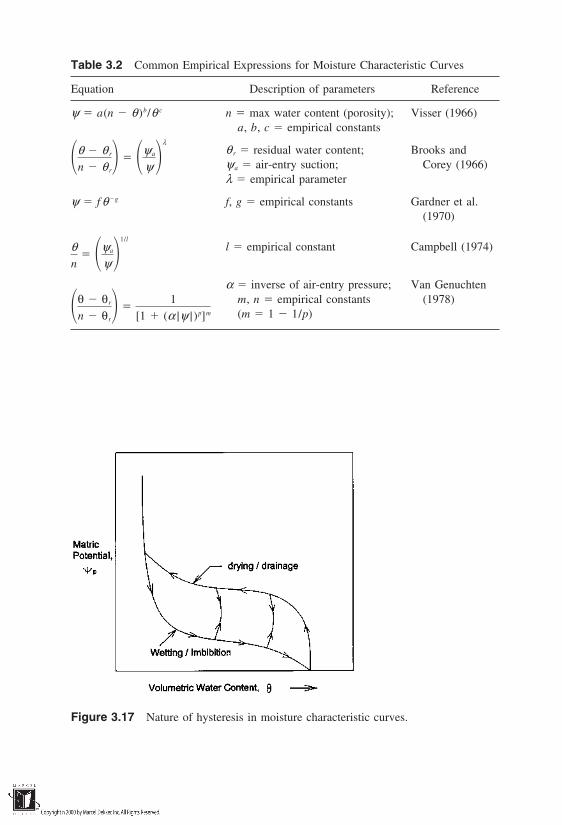
Table 3.2 Common Empirical Expressions for Moisture Characteristic Curves

Equation Description of parameters Reference

ψ a(n θ )b/θ c n max water content (porosity); Visser (1966)a, b, c empirical constants

θ r residual water content; Brooks andθ θ r

n θ r ψa

ψ λ

ψa air-entry suction; Corey (1966)λ empirical parameter

ψ f θg f, g empirical constants Gardner et al.(1970)

l empirical constant Campbell (1974)θn

ψa

ψ1/l

α inverse of air-entry pressure; Van Genuchtenm, n empirical constants (1978)θ θr

n θr

1[1 (α |ψ | )p]m (m 1 1/p)

Figure 3.17 Nature of hysteresis in moisture characteristic curves.

the drying and the wetting phases, and the pores tend to be interconnected indifferent ways in the two phases. The characteristic curve is called a drying ordrainage curve when the soil is incrementally dried from a saturated state, anda wetting or imbibition curve when the soil is wetted from an initially dry state.

3.6.2 Variation of Coefficient of Permeability with WaterContent

At a given state of unsaturated flow, not all capillary tubes participate in flow.The permeability of the unsaturated zone depends on the number and the sizesof the pore tubes participating in flow. Since water content θ is a direct reflectionof these parameters, it is obvious that the permeability of unsaturated soils de-pends on θ. From Poiseulle’s law discussed in Section 3.3.1, the flow rate througha capillary tube is directly proportional to the fourth power of radius of the tube.This means that flow rates are larger when large pores are conducting flow thanwhen small pores are conducting. Since large pores are associated with higherwater contents, it is clear that permeability increases with an increase in watercontent. A schematic variation of unsaturated permeability with respect to watercontent, for various soil types, is shown in Figure 3.18. At complete saturation(corresponding to θ n), coarser soils such as sands have higher permeabilitybecause of larger pore tubes. However, after these large pores are drained, perme-

Figure 3.18 Schematic variation of unsaturated permeability with respect to volumetricwater content.

ability decreases rapidly. The decrease in permeability is more gradual in thecase of fine-grained soils, such as clays.

We may represent the flow in a single capillary tube as we did in Section3.3.1, and sum up the contributions of all conducting tubes to obtain a relationfor unsaturated permeability. Assuming that there are K different radii of capillarytubes of length L, all of which are conducting flow, the total flow rate may beexpressed as

q π

8η ∆P

L K

i1

NiR4i (3.68)

where Ni the number of tubes of radius Ri per unit area of cross section. Toknow the number and size of tubes contributing to flow at a given unsaturatedstate, we use the moisture characteristic curve. The matric potential of an unsatu-rated soil can be transformed to pore tube radius using the capillarity equation(3.6). Consider the state of soil at a moisture content of θ1, which is less thanthe saturated water content (n) by a small increment, ∆θ. The volumetric watercontent θ1 corresponds to the state when ∆θ has been drained through tubes ofradius R1, which is given by 2σ cos α/ψp [Eq. (3.6)]. For a unit length of poretubes, ∆θ may be expressed as

∆θ N1πR21 (3.69)

which gives us an expression for the number of pores of radius R1 as

N1 ∆θπR2

1

(3.70)

Using this process, the number of pores contributing to flow can be obtained foran unsaturated soil at any state dryer than θ1 using small increments of ∆θ. Atwater content θ1, pores of radius R1 have all drained, and only those smaller thanR1 conduct flow. Expressing the number of pore tubes Ni in terms of ∆θ and Ri,the total flow rate corresponding to water content θ1 may be expressed as followsusing Eq. (3.68):

qu(θ1) 1

8η ∆P

L ∆θ K

i2

R2i (3.71)

By analogy with Darcy’s law, the permeability of the unsaturated soil, ku, maybe expressed as

ku(θ1) ∆θ8η

K

i2

R2i (3.72)

The radii can be transformed to the matric potentials [Eq. (3.6)], and the perme-ability can be expressed in terms of matric potentials as

ku(ψp1) σ 2 ∆θ

2η K

i2

1ψ 2

pi

(3.73)

Thus, a knowledge of the moisture characteristic curve can be theoretically usedto obtain an expression for the unsaturated permeability. As an alternative, theKozeny-Carmen equation derived in Section 3.3.2 may be used to obtain an ex-pression for unsaturated permeability in terms of void ratio and degree of satura-tion. Expressing Eqs. (3.21) and (3.22) in terms of the degree of saturation S, toaccount for the reduced flow area, the reader can deduce that

ku S3 (3.74)

Again, the above equations are more of theoretical importance because of thecapillary tube analogy used in their derivation. Similar to moisture characteristic

Table 3.3 Common Empirical Relationships for Unsaturated Permeability

Function Source

ku(ψ) a(b ψ n)1 Childs and Collis-George (1950)

ku(ψ) ks

1 ψψc

n

Gardner (1958)

ku(θ) k sθ θ r

θ s θ rn

Brooks and Corey (1966)

ku(ψ) a

ψBaver et al. (1972)

ku(ψ) ks exp(aψ) Mualem (1976)

ku(θ) a(θ)n Marshall and Holmes (1979)

Van Genuchten (1980)ku(θ) ks√θ θ r

θ s θ r1 1 θ θ r

θ s θ r

1/m

m

2

Note: ks saturated permeability; θ s volumetric water content at saturation (equal to porosity);ψc matric potential for which ku ks/2; θ r residual water content; and a, b, m, and n areempirical constants.

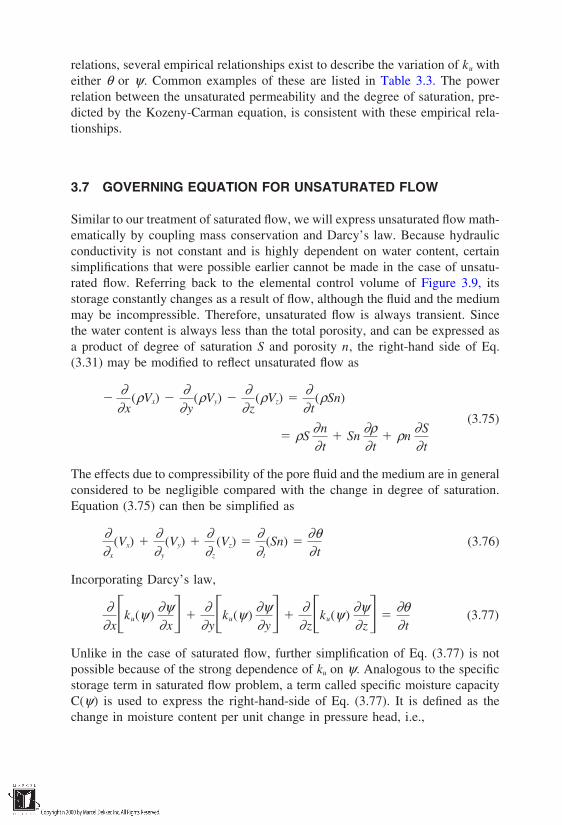
relations, several empirical relationships exist to describe the variation of ku witheither θ or ψ. Common examples of these are listed in Table 3.3. The powerrelation between the unsaturated permeability and the degree of saturation, pre-dicted by the Kozeny-Carman equation, is consistent with these empirical rela-tionships.

3.7 GOVERNING EQUATION FOR UNSATURATED FLOW

Similar to our treatment of saturated flow, we will express unsaturated flow math-ematically by coupling mass conservation and Darcy’s law. Because hydraulicconductivity is not constant and is highly dependent on water content, certainsimplifications that were possible earlier cannot be made in the case of unsatu-rated flow. Referring back to the elemental control volume of Figure 3.9, itsstorage constantly changes as a result of flow, although the fluid and the mediummay be incompressible. Therefore, unsaturated flow is always transient. Sincethe water content is always less than the total porosity, and can be expressed asa product of degree of saturation S and porosity n, the right-hand side of Eq.(3.31) may be modified to reflect unsaturated flow as

∂

∂x(ρVx)

∂∂y

(ρVy) ∂∂z

(ρVz) ∂∂ t

(ρSn)

ρS∂n

∂ t Sn

∂ρ∂ t

ρn∂S

∂ t

(3.75)

The effects due to compressibility of the pore fluid and the medium are in generalconsidered to be negligible compared with the change in degree of saturation.Equation (3.75) can then be simplified as

∂∂x

(Vx) ∂∂y

(Vy) ∂∂z

(Vz) ∂∂ t

(Sn) ∂θ∂ t

(3.76)

Incorporating Darcy’s law,

∂∂xku(ψ)

∂ψ∂x

∂∂yku(ψ )

∂ψ∂y

∂∂zku(ψ )

∂ψ∂z

∂θ∂ t

(3.77)

Unlike in the case of saturated flow, further simplification of Eq. (3.77) is notpossible because of the strong dependence of ku on ψ. Analogous to the specificstorage term in saturated flow problem, a term called specific moisture capacityC(ψ) is used to express the right-hand-side of Eq. (3.77). It is defined as thechange in moisture content per unit change in pressure head, i.e.,

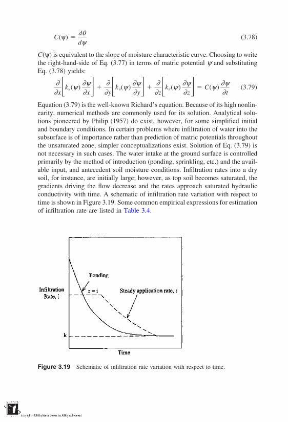
C(ψ) dθdψ

(3.78)

C(ψ) is equivalent to the slope of moisture characteristic curve. Choosing to writethe right-hand-side of Eq. (3.77) in terms of matric potential ψ and substitutingEq. (3.78) yields:

∂∂xku(ψ)

∂ψ∂x

∂∂yku(ψ )

∂ψ∂y

∂∂zku(ψ )

∂ψ∂z C(ψ)

∂ψ∂ t

(3.79)

Equation (3.79) is the well-known Richard’s equation. Because of its high nonlin-earity, numerical methods are commonly used for its solution. Analytical solu-tions pioneered by Philip (1957) do exist, however, for some simplified initialand boundary conditions. In certain problems where infiltration of water into thesubsurface is of importance rather than prediction of matric potentials throughoutthe unsaturated zone, simpler conceptualizations exist. Solution of Eq. (3.79) isnot necessary in such cases. The water intake at the ground surface is controlledprimarily by the method of introduction (ponding, sprinkling, etc.) and the avail-able input, and antecedent soil moisture conditions. Infiltration rates into a drysoil, for instance, are initially large; however, as top soil becomes saturated, thegradients driving the flow decrease and the rates approach saturated hydraulicconductivity with time. A schematic of infiltration rate variation with respect totime is shown in Figure 3.19. Some common empirical expressions for estimationof infiltration rate are listed in Table 3.4.

Figure 3.19 Schematic of infiltration rate variation with respect to time.

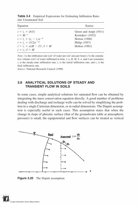
Table 3.4 Empirical Expressions for Estimating Infiltration Ratesinto Unsaturated Soil

Equation Source

i ic (b/I ) Green and Ampt (1911)i Bt n Kostiakov (1932)i ic (io ie)ekt Horton (1940)i ie (3/2)t 1/2 Philip (1957)i ic a(M I )n; I M Holton (1961)i ic; I M

Note: i is the infiltration rate (cm3 of water per cm2 area per hour); I is the cumula-tive volume (cm3) of water infiltrated in time, t; a, B, M, S, n, and k are constants;ic is the steady-state infiltration rate; ie is the initial infiltration rate; and io is thefinal infiltration rate.Source: National Research Council (1990)

3.8 ANALYTICAL SOLUTIONS OF STEADY ANDTRANSIENT FLOW IN SOILS

In some cases, simple analytical solutions for saturated flow can be obtained byintegrating the mass conservation equation directly. A good number of problemsdealing with discharge and recharge wells can be solved by simplifying the prob-lem in a single Cartesian dimension, or in radial dimensions. The Dupuit assump-tion is especially useful in such cases. This assumption states that when thechange in slope of phreatic surface (that of the groundwater table at atmosphericpressure) is small, the equipotential and flow surfaces can be treated as vertical

Figure 3.20 The Dupuit assumption.

Table 3.5 Analytical Solutions for Steady and Transient Flow in Soils

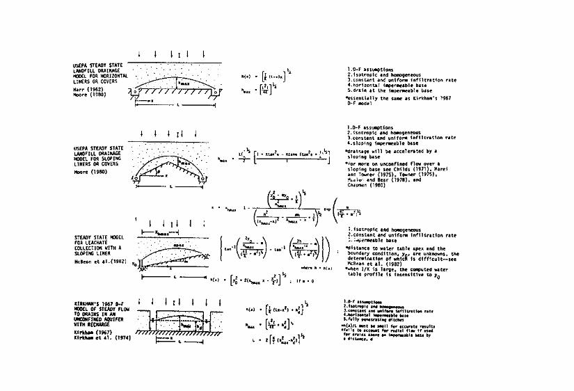
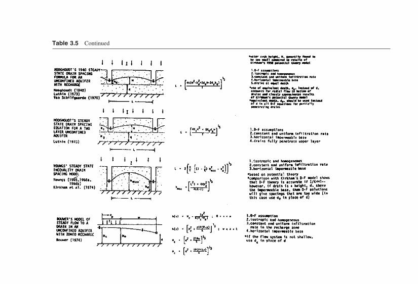
Table 3.5 Continued

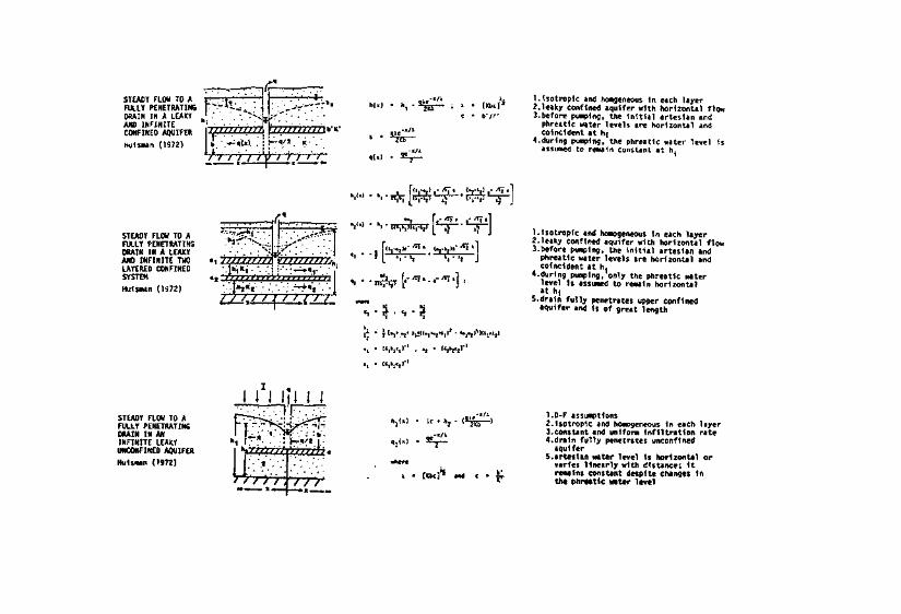
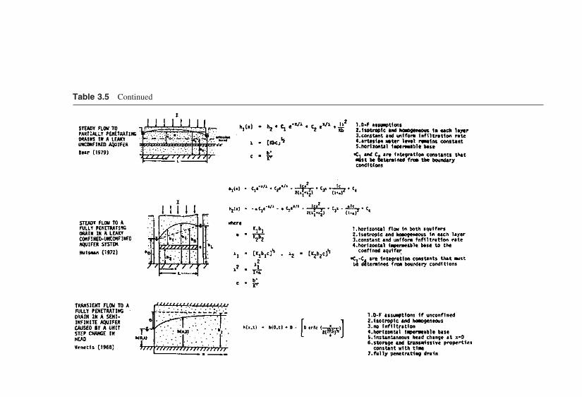
Table 3.5 Continued

Table 3.5 Continued

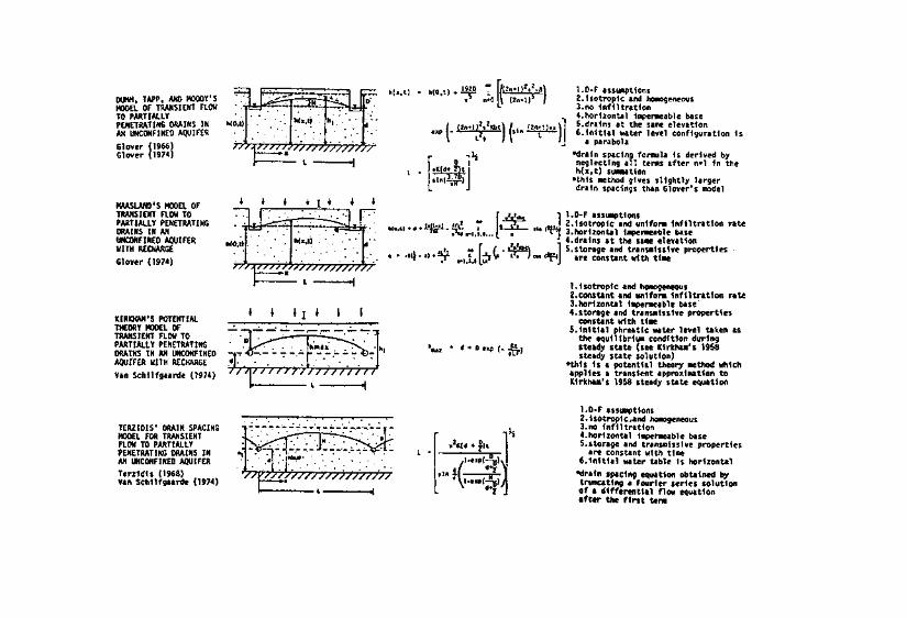
Table 3.5 Continued

Source: Cohen and Miller (1983).

and horizontal, respectively (Fig. 3.20). Bear (1972) has shown that the error dueto this assumption is small when i2 1, where i is the slope of the phreaticsurface. The scenarios where this assumption would lead to simple and usefulsolutions are shown in Table 3.5. Many of the solutions listed in Table 3.5 wereobtained assuming that the velocity of flow in the aquifer is proportional to theslope of the water table. Flow in the unsaturated zone is not considered in thesesolutions, and the infiltration to the groundwater table is generally considered asequal to the rate of application at the ground surface. We will find many of thesesolutions useful in site remediation activities and in designing drainage facilitiesfor waste containment systems, as discussed later in this book.

REFERENCES

Aslyng, H. C. (1963). Soil physics terminology. In. Soc. Soil Sci. Bull., 23:7.Baver, L. D., Gardner, W. H., and Gardner, W. R. (1972). Soil Physics. Wiley, New York.Bear, J. (1972). Dynamics of Fluids in Porous Media. American Elsevier, New York.Bear, J. (1979). Hydraulics of Ground Water. McGraw-Hill, New York.Benson, C. H., and Daniel, D. E. (1990). Influence of clods on hydraulic conductivity of

compacted clay. ASCE J. Geotech. Eng., 116(8):1231–1248.Boutwell, G. P., and Rauser, C. L. (1990). Clay liner construction. Geotechnical Engi-

neering in Today’s Environment, conference sponsored by the Central PennsylvaniaSection American Society of Civil Engineers, Hershey, PA, April 10–11, 1990.

Bouwer, H. (1974). Design and operation of land treatment systems for minimum contami-nation of ground water. Ground Water, 12(3):140–147.

Boynton, S. S., and Daniel, D. E. (1985). Hydraulic conductivity tests on compacted clay.ASCE J. Geotech. Eng. 111(4):465–477.

Brooks, R. H. (1961). Unsteady flow of ground water into drain tile. ASCE Proc., 87:27–37.

Brooks, R. H., and Corey, A. T. (1966). Properties of porous media affecting fluid flow.Proc. Am. Soc. Civ. Eng., J. Irrigation Drainage Div., IR2:61–88.

Campbell, G. S. (1974). A simple method for determining unsaturated conductivity frommoisture retention data. Soil Sci. 117(6):311–314.

Carman, P. C. (1956). Flow of Gases Through Porous Media. Academic Press, New York.Cedergren, H. R. (1989). Seepage, Drainage, and Flow Nets, 3rd ed. J Wiley, New York.Chauhan, H. S., Schwab, G. O., and Hamdy, M. Y. (1968). Analytical and computer solu-

tions of transient water tables for drainage of sloping land. Water Resources Res.4(3):573–579.

Childs, E. C., and Collis-George, N. (1950). The permeability of porous materials. Proc.R. Soc. London, A201:392–405.

Cohen, R. M., and Miller, W. J. (1983). Use of analytical models for evaluating correctiveactions at hazardous waste disposal facilities. Proceedings of the Third NationalSymposium on Aquifer Restoration and Ground Water Monitoring. National WaterWell Association, Worthington, OH, pp. 85–97.

Cooper, H. H., Jr., and Rorabaugh, M. I. (1963). Groundwater movements and bank stor-age due to flood stages in surface streams. USGS Water Supply Paper 1536-J, pp.352–357.

Daniel, D. E. (1984). Predicting hydraulic conductivity of clay liners. ASCE J. Geotech.Eng., 110:285–300.

Daniel, D. E. (1987). Earthen liners for land disposal facilities. In: R. D. Woods (ed.),Geotechnical Practice for Waste Disposal, Geotechnical Special Publication No.13, ASCE, pp. 21–39.

Daniel, D. E. (1994). State-of-the-Art: Laboratory Hydraulic Conductivity tests for satu-rated soils. In: D. E. Daniel and S. J. Trautwein (eds.), Hydraulic Conductivity andWaste Contaminant Transport in Soil, STP1142, ASTM, pp. 30–78.

Daniel, D. E., and Benson, C. H. (1990). Water content-density criteria for compactedsoil liners. ASCE J. Geotech. Eng., 116(12):1811–1830.

Day, S. R., and Daniel, D. E. (1985). Hydraulic conductivity of two prototype clay liners.ASCE J. Geotech. Eng., 111(8):957–970.

Ferris, J. G., Knowles, D. B., Brown, R. H., and Stallman, R. W. (1962). Theory of aquifertests. USGS Water Supply Paper 1536E.

Foreman, D. E., and Daniel, D. E. (1986). Permeation of compacted clay with organicchemicals. ASCE J. Geotech. Eng., 112(7).

Freeze, R. A., and Cherry, J. A. (1979). Groundwater. Prentice Hall, Englewood Cliffs,NJ.

Gardner, W. R. (1958). Some steady-state solutions of the unsaturated moisture flow equa-tion with application to evaporation from a water table. Soil Sci. 85(4):228–232.

Gardner, W. R., Hillel, D., and Benyamini, Y. (1970). Post irrigation movement of soilwater. I. Redistribution. Water Resources Res., 6(3):851–861; II. Simultaneous re-distribution and evaporation. Water Resources Res., 6(4):1148–1153.

Glover, R. E. (1966). Theory of Ground-Water Movement. U. S. Bureau of ReclamationEngineering Monograph No. 31.

Glover, R. E. (1974). Transient Ground-Water Hydraulics. Water Resources Publications,Fort Collins, Co.

Green, W. H., and Ampt, G. A. (1911). Studies on soil physics, I. Flow of air and waterthrough soils. J. Agr. Sci., 4:1–24.

Hantush, M. S. (1967). Growth and decay of ground-water mounds in response to uniformpercolation. Water Resources Res. 3(1):227–234.

Harr, M. E. (1962). Ground-Water and Seepage. McGraw-Hill, New York.Hazen, A. (1911). Discussion of ‘‘Dams on Sand Foundation’’ by A. C. Koenig, Trans.

ASCE, 73:199.Holton, H. N. (1961). A Concept of Infiltration Estimates in Watershed Engineering, Ag-

ricultural Research Service Publication 41–51. U. S. Department of Agriculture,Washington, DC.

Hooghoudt, S. B. (1940). Bijdragen tot de kennis van eenige natuurkundige groothedenvan den grond, 7. Algemeene beschouwing van het probleem van de detail ontwater-ing en de infiltratie door middel van parallel loopende drains, greppels, slooten, enkanalen. Versl. Landbouwk. Ond., 46:515–707.

Horton. (1940). An approach toward a physical interpretation of infiltration capacity. SoilSci. Soc. Am. Proc., 5:399–417.

Huisman, L. (1972). Ground-Water Recovery. Winchester Press, New York.Jacob, C. E. (1943). Correlation of ground-water levels with precipitation on Long Island,

New York. Ann. Geophys. Union Trans., pt. 2:564–573.Kirkham, D. (1958). Seepage of steady rainfall through soil into drains. Am. Geophys.

Union Trans., 39:892–908.Kirkham, D. (1967). Explanation of paradoxes in the Dupuit-Forchheimer seepage theory.

Water Resources Res., 3:609–622.Kirkham, D., Toksoz, S., and van der Ploeg, R. R. (1974). Steady flow to drains and wells.

In J. van Schilfgaarde (ed.) Drainage for Agriculture, pp. 203–244. American Soci-ety of Agronomy, Madison, WI.

Kostiakov, A. N. (1932). On the dynamics of the coefficient of water percolation in soilsand on the necessity of studying it from a dynamic point of view for purposes ofamelioration. Transactions Com. International Soil Science, 6th, Moscow, Russia,Part A, pp. 17–21.

Kozeny, J. (1927). Ueber kapillare Leitung des Wassers im Boden, Wien. Akad. Wiss.,136, pt 2a:271.

Lambe, T. W., and Whitman, R. V. (1969). Soil Mechanics. Wiley, New York.Luthin, J. N. (1973). Drainage Enginering. R. E. Krieger, Huntington, NY.Marshall, T. J., and Holmes, J. W. (1979). Soil Physics. Cambridge University Press, New

York.McBean, E. A., Poland, R., Rovers, F. A., and Crutcher, A. J. (1982). Leachate collection

design for containment landfills. ASCE J. Env. Eng. Div., 108(1):204–209.Mitchell, J. K., Hooper, D. R., and Campanella, R. G. (1965). Permeability of compacted

clay. ASCE J. Soil Mech. Found. Div., 91(SM4), Proceedings Paper 4392.Mitchell, J. K., and Madsen, F. T. (1987). Chemical effects on clay hydraulic conductivity.

In Woods R. D. (ed.), Geotechnical Practice for Waste Disposal, Geotechnical Spe-cial Publication No. 13, ASCE, pp. 87–116.

Moody, W. T., and Ribbens, R. W. (1965). Ground water—Tetrama-Colusa canal reachno. 3, Sacramento Canal Units, Central Valley Project. Memorandum to Chief, Ca-nals Branch. Bureau of Reclamation, Office of Chief Engineer, Denver, Co.

Moore, C. A. (1980). Landfill and Surface Impoundment Performance Evaluation. U.S.EPA SW-869.

Mualem, Y. (1976). Hysteretical models for prediction of the hydraulic conductivity ofunsaturated porous media. Water Resources Res., 12:1248–1254.

National Research Council (1990). Groundwater models: Scientific and regulatory applica-tions. National Academy Press, Washington, DC.

Philip, J. R. (1957). The theory of infiltration, 4. Sorptivity and algebraic infiltration equa-tions. Soil Sci., 84:257–264.

Richards, S. J. (1965). Soil suction measurements with tensiometers. In Methods of SoilAnalysis, Monograph 9, pp. 153–163. American Society of Agronomy, Madison,WI.

Singh, S. R., and Jacob, C. M. (1977). Transient analysis of phreatic aquifers lying betweentwo open channels. Water Resources Res., 13(2) 411–419.

Slatyer, R. O. (1967). Plant–Water Relationships. Academic Press, New York.Swartzendruber, D. (1962). Non-Darcy flow behavior in liquid-saturated porous media.

J. Geophys. Res., 67:5205–5213.

Terzaghi, K. (1925). Erdbaumechanik auf Boden-physicalischen Grundlagen. Deuticke,Vienna.

Terzidis, G. (1968). Discussion, falling water table between tile drains. ASCE Proc. 94:159.

U. S. Department of the Interior. (1981). Ground-Water Manual. U. S. Department of theInterior.

Van Genuchten, R. (1978). Calculating the unsaturated hydraulic conductivity with a newclosed-form analytical model. Publication of the Water Resourses Program, Depart-ment of Civil Engineering, Princeton University Princeton, NJ.

Van Genuchten, M. Th. (1980). A closed-form equation for predicting the hydraulic con-ductivity of unsaturated soils. Soil Sci. Soc. Am. J. 44:892–898.

Van Schilfgaarde, J. (1970). Theory of flow to drains. In Advances in Hydroscience, vol.6, pp. 43–106. Academic Press, New York.

Van Schilfgaarde, J. (1974). Nonsteady flow to drains. In J. van Schilfgaarde ed., Drainagefor Agriculture, pp. 245–270. American Society of Agronomy, Madison, WI.

Venetis, C. (1968). On the impulse response of an aquifer. Bull. Int. Assoc. Sci. Hydrol.13:136–139.

Visser, W.C. (1996). Progress in the knowledge about the effect of soil moisture contenton plant production. Inst. Land Water Management, Wageningen, Netherlands,Tech. Bull. 45.

Youngs, E. G. (1965). Horizontal seepage through unconfined aquifers with hydraulicconductivity varying with depth. J. Hydrol., 3:448–451.

Youngs, E. G. (1966a). Horizontal seepage through unconfined aquifers with nonuniformhydraulic conductivity. J. Hydrol., 4:91–97.

Youngs, E. G. (1966b). Exact analysis of certain problems of ground-water flow with freesurface conditions. J. Hydrol., 4:227–281.

4Mass Transport and Transferin Soils

4.1 INTRODUCTION

In this chapter, we will address the issue of how contaminants migrate in thesubsurface relative to pore water while simultaneously interacting with eachother. We note that contaminants participate in several physical, chemical, andbiological transformation processes during the course of their travel. These trans-formation processes should be taken into account in the assessment of soil andgroundwater quality. As we will see later in this book, knowledge of contaminanttransport and transfer in soils is crucial in site remediation and waste containmentefforts.

As noted in Chapter 3, any formulation for transport in porous media essen-tially involves application of the mass conservation principle and cause-and-ef-fect relationships in the form of constitutive equations. The mass conservationprinciple applied to contaminants in an elemental volume of porous media dic-tates that

(Rate of mass input) (rate of mass output)

(rate of mass production or consumption) (4.1)

rate of mass accumulation

where the addition and subtraction on the left-hand side (l.h.s.) apply to massproduction and consumption, respectively. Mass transfer processes contribute tomass consumption or production in porous media and thus directly relate to thesink/source terms in Eq. (4.1). Mass transport processes, on the other hand, enteras constitutive relations in our formulation. We will see that the transport pro-cesses involve not only the application of Darcy’s law (elaborated in Chapter 3),but also Fick’s law discussed subsequently.

We need to make an important distinction between contaminants that are

soluble in water and those that are insoluble or immiscible in water. The twotypes of contaminants differ in the way their transport takes place relative to porewater. The transport of soluble contaminants is more closely linked to the flowof pore water than that of immiscible contaminants, which is governed by a hostof pore-scale and field-scale mechanisms not related to flow of water. We willdefer discussion of immiscible contaminants to the next chapter and take up thedissolved contaminants first.

4.2 MASS TRANSPORT MECHANISMS

The transport of dissolved contaminants follows that of water via advection andis therefore related to the velocity of water flow. The direction of hydraulic gradi-ents dictates to a large extent the direction of dissolved contaminant transport.If advection is the only mechanism of transport, the pore velocity (Darcy velocitydivided by porosity) is an indicator of the transport of dissolved contaminants.Thus, when a chemical with a concentration of C0 is introduced into a saturatedsoil system as shown in Figure 4.1a, it migrates as a sharp front at a velocityequal to the pore velocity, Va. In reality, however, there are other mechanismsaugmenting advection. The saturated soil system possesses concentration gradi-ents in addition to hydraulic gradients because of the localized presence of the

Figure 4.1 Chemical transported in groundwater: (a) via advection; (b) via advectionand diffusion.

dissolved chemical. These concentration gradients exercise kinetic activity andprovide for an additional mechanism of transport namely, diffusion. As shownschematically in Figure 4.1b, the effect of diffusion is to cause the contaminantto be spread out in all directions in response to concentration gradients. Therelative contributions of advection and diffusion are therefore dependent on themagnitudes of velocity and the concentration gradients. In systems where veloci-ties are low (by virtue of low permeability, such as in the case of waste-contain-ment barriers), one can expect diffusion process to dominate. On the other hand,in systems where flow velocities are high, such as in coarse-grained soils, advec-tion dominates. Leaving the quantitative analysis of these relative contributionsto a later stage, we start with a discussion of the diffusion process.

Fick’s first law provides us with a formal representation of the diffusionprocess. Analogous to Darcy’s law, it states that the flux of diffusing chemical,J, (mass of solute per unit area per unit time, M/L2T) is directly proportional tothe concentration gradient:

J D*dC

dx(4.2)

where C is the solute concentration (M/L3), D* is the diffusion coefficient for thesoil medium (L2/T), and dC/dx is the concentration gradient, which is negative inthe direction of diffusion. D* is thus a coefficient of proportionality analogousto the coefficient of permeability k in Eq. (3.16). Carrying the analogy betweenthe coefficients of permeability and diffusion further, the measurement of diffu-sion coefficients is also often indirect. Concentration gradients are applied overa soil sample and the observed chemical flux is used in Fick’s first law to deter-mine the diffusion coefficient D*. Efforts to obtain a direct expression for diffu-sion coefficient in terms of the soil and pore fluid parameters were based onextrapolations of free-solution diffusion, as discussed below.

The fundamental basis for deriving an expression for the free-solution dif-fusion coefficient is the mobility of ions as determined by their mass, radius, andvalence, and by the properties of the liquid, such as viscosity, dielectric constant,and temperature. Three expressions derived from fundamental principles aregiven below.

Do uRT

NNernst-Einstein equation (4.3)

Do RTλo

F 2 |z|Nernst equation (4.4)

Do RT

6πNηrEinstein-Stokes equation (4.5)

where Do is the free-solution diffusion coefficient; u absolute mobility of thesolute; R universal gas constant; T absolute temperature; N Avogadro’snumber (6.022 1023 mol1); λo limiting ionic conductivity; F Faradayconstant (96,500 C/Eq); |z| absolute value of the ionic valence; η viscosityof the fluid; and r radius of the molecular or hydrated ion. These equationswere all based on the same principles of ionic mobility. The absolute mobilityof the solute, u, is expressed in terms of ionic conductivity λo in Eq. (4.4) andin terms of the size of the ion and the viscosity of the fluid in Eq. (4.5). Thediffusion of species in a free solution is thus a complex function of a number ofvariables, viz, ionic radius, valence, temperature, viscosity of the diffusing me-dium, etc. Typical values of Do for selected anions and cations are shown inTable 4.1. Values for other species may be found in Lerman (1979), and in Liand Gregory (1974).

The diffusion coefficient for a species in porous medium will be smallerthan that in free solution, primarily because of the limited domain available forionic flow. An effective diffusion coefficient, D*, in soils may therefore be ex-pressed as

D* ωDo (4.6)

where ω is an empirical constant (typically ranging from 0.5 to 0.01) accountingfor the presence of soil solids in the medium. More rigorous ways of accountingfor the various factors involved in the diffusion process in soils are reviewed by

Table 4.1 Free-Solution Diffusion Coefficients forSelected Speciesa

D0 1010 D0 1010

Cation (m2/s) Anion (m2/s)

H 93.1 OH 52.8Na 13.3 Cl 20.3K 19.6 F 14.7NH4

19.8 Br 20.8Mg2 7.1 I 20.4Ca2 7.9 NO3

19.0Fe2 7.2 HCO3

11.8Cu2 7.3 SO4

2 10.7Zn2 7.2 CO3

2 9.6

a Values correspond to infinite dilution in water at 25°C.Sources: Li and Gregory (1974); Lerman (1979).

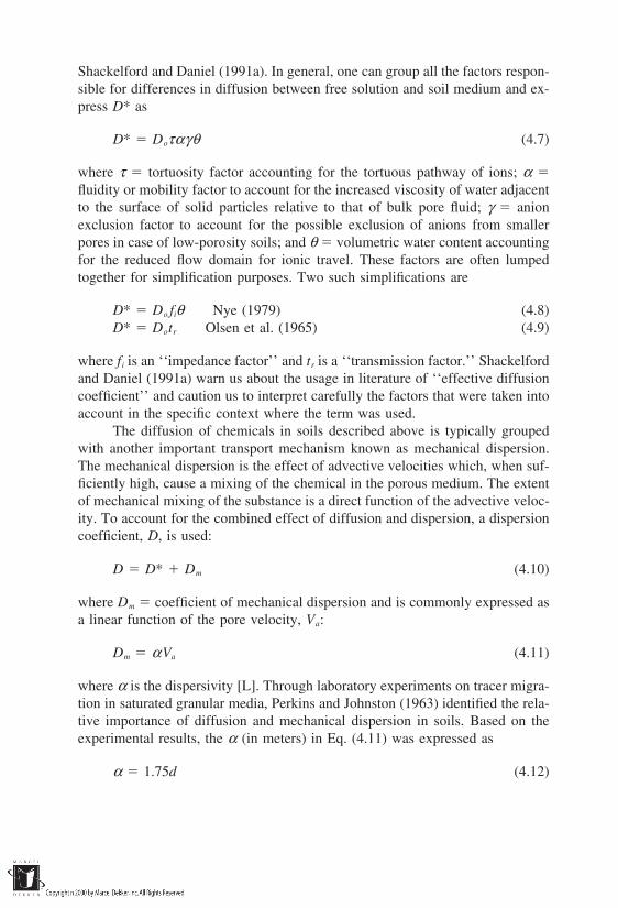
Shackelford and Daniel (1991a). In general, one can group all the factors respon-sible for differences in diffusion between free solution and soil medium and ex-press D* as

D* Doταγθ (4.7)

where τ tortuosity factor accounting for the tortuous pathway of ions; α fluidity or mobility factor to account for the increased viscosity of water adjacentto the surface of solid particles relative to that of bulk pore fluid; γ anionexclusion factor to account for the possible exclusion of anions from smallerpores in case of low-porosity soils; and θ volumetric water content accountingfor the reduced flow domain for ionic travel. These factors are often lumpedtogether for simplification purposes. Two such simplifications are

D* Do fiθ Nye (1979) (4.8)D* Dotr Olsen et al. (1965) (4.9)

where fi is an ‘‘impedance factor’’ and tr is a ‘‘transmission factor.’’ Shackelfordand Daniel (1991a) warn us about the usage in literature of ‘‘effective diffusioncoefficient’’ and caution us to interpret carefully the factors that were taken intoaccount in the specific context where the term was used.

The diffusion of chemicals in soils described above is typically groupedwith another important transport mechanism known as mechanical dispersion.The mechanical dispersion is the effect of advective velocities which, when suf-ficiently high, cause a mixing of the chemical in the porous medium. The extentof mechanical mixing of the substance is a direct function of the advective veloc-ity. To account for the combined effect of diffusion and dispersion, a dispersioncoefficient, D, is used:

D D* Dm (4.10)

where Dm coefficient of mechanical dispersion and is commonly expressed asa linear function of the pore velocity, Va:

Dm αVa (4.11)

where α is the dispersivity [L]. Through laboratory experiments on tracer migra-tion in saturated granular media, Perkins and Johnston (1963) identified the rela-tive importance of diffusion and mechanical dispersion in soils. Based on theexperimental results, the α (in meters) in Eq. (4.11) was expressed as

α 1.75d (4.12)

Figure 4.2 Relative effects of molecular diffusion and mechanical dispersion on thedispersion coefficient, D. (Source: Perkins and Johnston, 1963)

where d is the mean grain diameter of the soil in meters. Figure 4.2 shows thevariation of D with respect to the actual velocity, Va, for the two extreme condi-tions of D* and d. In fine soils with high diffusion, D* alone controls the disper-sion coefficient; on the other hand, in coarse soils with a low diffusion, D iscontrolled by mechanical dispersion for velocities greater than 1 m per year. Itis customary in practice to substitute D for D* in Eq. (4.2); however, the readermay question the validity of lumping mechanical dispersion with a constant ofproportionality between mass flux and concentration gradient.

In the case of engineered systems such as compacted clays, the above prin-ciples are generally taken to be valid. Unlike the permeability aspect, the diffusionbehavior of compacted clays has been addressed in only a few studies (Quigleyet al., 1987; Shackelford and Daniel, 1991b). These studies indicate that diffusionplays an important role in the breakthrough of chemicals through compactedclays. They suggest that the experimental errors far outweigh any variability ofeffective diffusion coefficient with respect to molding water content and type ofcompaction. Diffusion in compacted clays is still an area of active research, andfuture studies may lead to further understanding of the process.

4.3 MASS TRANSFER MECHANISMS

A specific chemical element or compound may exist in groundwater in any ofthe following forms (Johnson et al., 1989):

1. As ‘‘free’’ ions surrounded by water molecules2. As insoluble species, e.g., Ag2S, BaSO4

3. As metal–ligand complexes, e.g., Al(OH)2

4. As adsorbed species5. As species held on a surface by ion exchange6. As species that differ by oxidation state, e.g., Fe2, Fe3; Cr3, Cr4

The various chemicals existing in one or more of these forms, while participatingin reactions with each other to achieve equilibrium, may transfer from one phaseto the other among the three phases—solids, liquids, and gases. In other words,the reactions can be homogeneous (occurring in only one phase) or heterogeneous(involving phase transfer). The transformation of a chemical from its initial stateis an intricate process, which constantly influences and is influenced by the trans-port mechanisms. Furthermore, change in state of one species may alter the masstransfer mechanisms of other species. It is here that one would find it necessaryto augment a mass transport model with a geochemical model, which considersthe myriad changes that a chemical in the subsurface undergoes during the courseof its migration.

While some transfer mechanisms are better understood than others, manyof the mechanisms are still actively being researched in the field of geochemistry.Our purpose in the following subsections is to obtain knowledge of the individualmass transfer mechanisms to the extent needed to understand the transport phe-nomena in soils. An important consideration in transport modeling is the rate atwhich the various transfer processes occur in soils. The time period required fora specific transfer process relative to that of advection and diffusion processes willgovern the significance of that process in transport modeling. Thus, the transferprocesses, which take place at time scales far greater than those required by ad-vection and diffusion, can safely be ignored in transport modeling. Unfortunately,this is not true for a majority of the processes, which have reaction rates muchgreater than the typical rates of groundwater flow—hence the need for a detaileddiscussion of these processes. We will take up the issue of reaction times afterdiscussing briefly the individual mechanisms.

It is convenient to treat the mass transfer mechanisms under two groups:(1) abiotic processes; and (2) biotic processes. The abiotic processes refer to thosethat are nonbiological in nature. The biotic processes involve mass consumptionof the chemicals by microorganisms, often referred as biodegradation. The popu-

lation growth/decline of microorganisms in the presence of various chemicals isof primary importance in these processes. In reality, both abiotic and biotic pro-cesses occur concurrently. The microorganisms involved in the biotic processesact as catalysts for some of the reactions in abiotic processes.

4.3.1 Abiotic Processes

The major mechanisms under this classification are: (1) acid–base reactions, (2)hydrolysis, (3) oxidation–reduction (redox) reactions, (4) complexation, (5) pre-cipitation and dissolution, (6) exsolution and volatilization, (7) radioactive decay,and (8) sorption.

Acid–Base Reactions

Acid–base reactions are the most fundamental processes involving the exchangeof hydrogen ions (H). These reactions take place almost instantaneously be-tween substances tending to lose H ions (acids) and those tending to gain thesame (bases). They alter the pH of the system, which in turn affects other mecha-nisms such as sorption. Very often, it is this indirect effect of acid–base reactions(through changes in pH) that is of importance in transport modeling. Becauseof the pH changes, the chemicals participating in these reactions may influencetransport of contaminants, although the chemicals by themselves may not be thecontaminants of concern. The following are two examples of these reactions:

HCO3 H2O H3O CO3

2 (4.13)

NH3 H2O NH4 OH (4.14)

In the first reaction, water serves as the base accepting a proton, and in the secondreaction, it serves as the acid donating a proton. The acid–base reactions areoften referred as weak or strong depending on the extent of proton transfer. Sev-eral examples of acid–base reactions common to groundwater systems may befound in Morel (1983) and in Domenico and Schwartz (1990).

Hydrolysis

Hydrolysis is a mass transfer process that is a result of substitution between anorganic compound and water. It may be represented as

(R X) H2O → (R OH) X H (4.15)

where R refers to the main part of organic molecule and X represents the attachedhalogen, carbon, phosphorous, or nitrogen. The introduction of hydroxyl into theorganic molecule may make the reaction product more soluble and susceptibleto biodegradation. Thus, hydrolysis may be an important transfer mechanism in

remediation efforts, since it may transform an organic compound, originally resis-tant to biodegradation, to a degradable compound. However, not all organic com-pounds participate in hydrolysis reactions. Those which are susceptible to hydro-lysis include alkyl halides, amides, carbamates, carboxylic acid esters, epoxidesand lactones, phosphoric acid esters, and sulfonic acid esters (Neely, 1985).

Oxidation–Reduction (Redox) Reactions

Oxidation–reduction reactions involve exchange of electrons, similar to exchangeof protons in the case of acid–base reactions. Oxidation and reduction refer tothe removal and acceptance of electrons, respectively. Examples of these reac-tions are

Fe2 Fe3 e (4.16)

Fe3 e Fe2 (4.17)

Equation (4.16) involves oxidation of Fe2, which donates an electron, and Eq.(4.17) involves reduction of Fe3, which accepts an electron. These reactionsessentially alter the oxidation number of elements. The oxidation number of iron,for instance, changes from 2 to 3 in the reaction shown in (4.16). It is importantto note, however, that no free electrons result from these reactions, since electronsgiven up by one compound are gained by another compound. The followingdescribes a complete redox reaction:

O2 4Fe2 4H 2H2O 4Fe3 (4.18)

wherein iron and oxygen participate as the electron donor (reductant) and electronacceptor (oxidant), respectively. The oxidation number of oxygen changes from0 to 2 and that of iron changes from 2 to 3. In general, any element that canhave different valencies may participate in redox reactions. Several trace elementshave variable oxidation numbers. Common elements found in variable oxidationstates, and examples of ions formed from these elements, are shown in Table4.2.

An important feature that distinguishes redox reactions from others is thatthey can be mediated by microorganisms, which act as catalysts to these reactions.The energy that is released when the electrons are donated in the redox reactionsbecomes a source for the microbial cells to sustain and grow. The following isan example of a biologically mediated redox reaction, which involves oxidationof an organic compound, CH2O, and reduction of oxygen:

14

CH2O 14

O2 14

CO2 14

H2O (4.19)

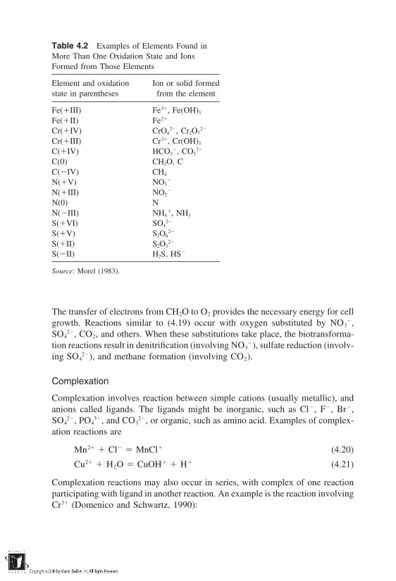
Table 4.2 Examples of Elements Found inMore Than One Oxidation State and IonsFormed from Those Elements

Element and oxidation Ion or solid formedstate in parentheses from the element

Fe(III) Fe3, Fe(OH)3

Fe(II) Fe2

Cr(IV) CrO42, Cr2O7

2

Cr(III) Cr3, Cr(OH)3

C(IV) HCO3, CO3

2

C(0) CH2O, CC(IV) CH4

N(V) NO3

N(III) NO2

N(0) NN(III) NH4

, NH3

S(VI) SO42

S(V) S2O62

S(II) S2O32

S(II) H2S, HS

Source: Morel (1983).

The transfer of electrons from CH2O to O2 provides the necessary energy for cellgrowth. Reactions similar to (4.19) occur with oxygen substituted by NO3

,SO4

2, CO2, and others. When these substitutions take place, the biotransforma-tion reactions result in denitrification (involving NO3

), sulfate reduction (involv-ing SO4

2), and methane formation (involving CO2).

Complexation

Complexation involves reaction between simple cations (usually metallic), andanions called ligands. The ligands might be inorganic, such as Cl, F, Br,SO4

2, PO43, and CO3

2, or organic, such as amino acid. Examples of complex-ation reactions are

Mn2 Cl MnCl (4.20)

Cu2 H2O CuOH H (4.21)

Complexation reactions may also occur in series, with complex of one reactionparticipating with ligand in another reaction. An example is the reaction involvingCr3 (Domenico and Schwartz, 1990):

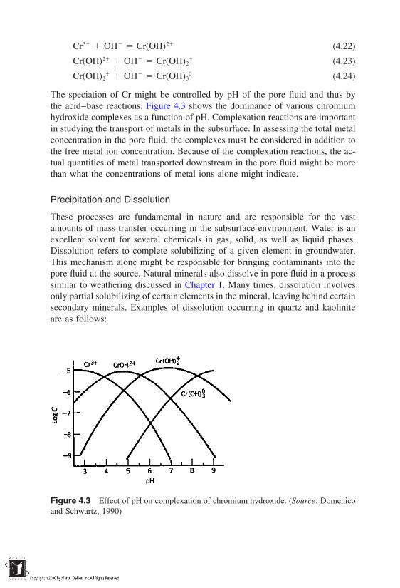
Cr3 OH Cr(OH)2 (4.22)

Cr(OH)2 OH Cr(OH)2 (4.23)

Cr(OH)2 OH Cr(OH)3

0 (4.24)

The speciation of Cr might be controlled by pH of the pore fluid and thus bythe acid–base reactions. Figure 4.3 shows the dominance of various chromiumhydroxide complexes as a function of pH. Complexation reactions are importantin studying the transport of metals in the subsurface. In assessing the total metalconcentration in the pore fluid, the complexes must be considered in addition tothe free metal ion concentration. Because of the complexation reactions, the ac-tual quantities of metal transported downstream in the pore fluid might be morethan what the concentrations of metal ions alone might indicate.

Precipitation and Dissolution

These processes are fundamental in nature and are responsible for the vastamounts of mass transfer occurring in the subsurface environment. Water is anexcellent solvent for several chemicals in gas, solid, as well as liquid phases.Dissolution refers to complete solubilizing of a given element in groundwater.This mechanism alone might be responsible for bringing contaminants into thepore fluid at the source. Natural minerals also dissolve in pore fluid in a processsimilar to weathering discussed in Chapter 1. Many times, dissolution involvesonly partial solubilizing of certain elements in the mineral, leaving behind certainsecondary minerals. Examples of dissolution occurring in quartz and kaoliniteare as follows:

Figure 4.3 Effect of pH on complexation of chromium hydroxide. (Source: Domenicoand Schwartz, 1990)

SiO2 H2O H2SiO3 (4.25)

Kaolinite 5H2O 2Al(OH)3 2H4SiO4 (4.26)

The dissolved components might be precipitated again due to reactions withother dissolved species. Some examples of chemicals that could be reduced tolower concentrations in the pore fluid through the formation of precipitates in-clude lead and silver, which enter into reactions with sulfides, carbonates, orchlorides. Precipitates may also be formed as the products of hydrolysis reactions(precipitates of iron, copper, chromium, and zinc) or redox reactions (precipitatesof chromium and arsenic). It is possible in certain cases that both precipitationand dissolution continue one after another as the plume moves downgradient.

Because of the pH dependence of speciation of metals (see Fig. 4.3), thesolubility of the metal oxides and hydroxides is also dependent on pH. Figure4.4 shows as examples the solubilities of zinc and copper as a function of pH.The lines on the graphs show the equilibrium conditions between solid and solu-ble forms of the metals. Thus the shaded portions of the plots show the cumulativesolubility for all the species of a given metal. The figure demonstrates that thereexists a pH at which the solubilities are minimum and beyond which the solubilityincreases again in the anionic form. The pH dependence of solubility is alsorelated to the specific type of the metal and the form of the precipitate. Figure4.5 shows the solubilities of certain metal oxides and sulfides, which shows thedifference in pH dependence between the solubilities of hydroxides and sulfides.

The solubility of organic solutes is highly variable. In general, chargedspecies of organic compounds or those containing oxygen or nitrogen are mostsoluble. An example is alcohols, which participate in hydrogen bonding with

Figure 4.4 Solubilities of zinc and copper as a function of pH. (Source: Stumm andMorgan, 1981)

Figure 4.5 Solubility of metal hydroxides and sulfides as a function of pH.

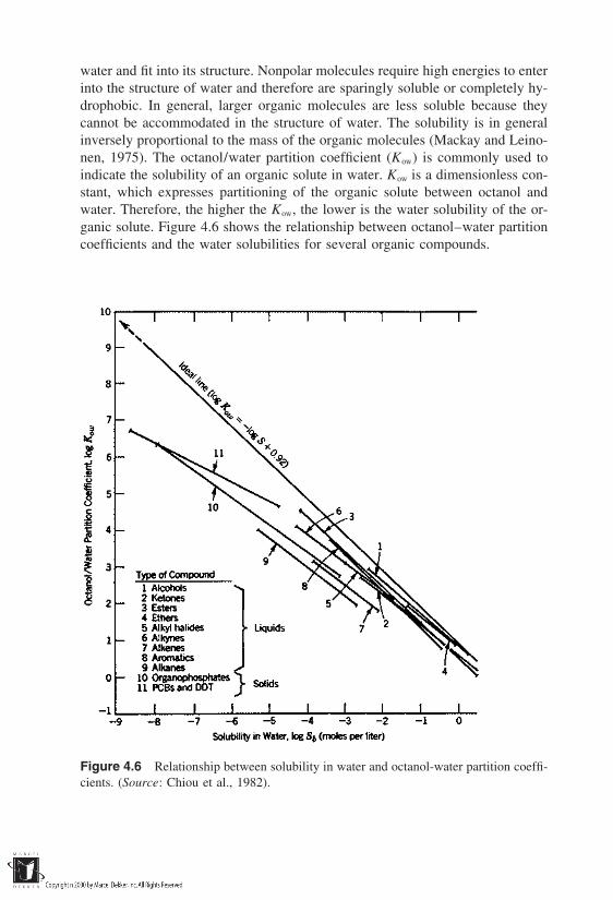
water and fit into its structure. Nonpolar molecules require high energies to enterinto the structure of water and therefore are sparingly soluble or completely hy-drophobic. In general, larger organic molecules are less soluble because theycannot be accommodated in the structure of water. The solubility is in generalinversely proportional to the mass of the organic molecules (Mackay and Leino-nen, 1975). The octanol/water partition coefficient (Kow) is commonly used toindicate the solubility of an organic solute in water. Kow is a dimensionless con-stant, which expresses partitioning of the organic solute between octanol andwater. Therefore, the higher the Kow, the lower is the water solubility of the or-ganic solute. Figure 4.6 shows the relationship between octanol–water partitioncoefficients and the water solubilities for several organic compounds.

Figure 4.6 Relationship between solubility in water and octanol-water partition coeffi-cients. (Source: Chiou et al., 1982).

Exsolution and Volatilization

These processes involve mass transfer between gaseous and either liquid or solidphases. Similar to precipitation, these processes remove mass from the pore waterinto the gaseous phase. They are controlled by the vapor pressure, which is thepressure of the gas in equilibrium with respect to the liquid or solid at a giventemperature. Vapor pressure reflects the solubility of a compound in gas and istherefore an indicator of the compound’s tendency to evaporate. The process isgoverned by two well-known laws, Raoults’ law and Henry’s law. The formeris used to relate the equilibrium partial pressure of a volatile organic in the atmo-sphere to the pure constituent vapor pressure. In other words,

Pi xiPi0 (4.27)

where Pi partial pressure of the vapor in the gas phase; xi mole fraction ofthe organic solvent; and Pi

0 vapor pressure of the pure organic solvent. Equa-tion (4.27) is applicable only when the mole fraction of the solvent is greaterthan 0.9, and is therefore valid to represent volatilization of pure solvents. Todescribe volatilization of many solutes dissolved in water, Henry’s law is usedinstead. It relates the equilibrium partial pressure of a constituent directly to themole fraction of the constituent in the aqueous phase. It is expressed as

Pi HiXi (4.28)

where Pi partial pressure of the vapor in the gas phase; Xi mole fraction ofthe constituent in the aqueous phase, and Hi Henry’s constant specific for theconstituent. As seen in Eq. (4.28), Henry’s constant is an indicator of the ratioof constituent concentration in the vapor phase to that in the aqueous phase.Table 4.3 lists the vapor pressures and Henry’s constants for selected group ofcompounds.

Radioactive Decay

Radioactive decay is the process whereby unstable isotopes (atoms of the sameelement that differ in their mass) decay to form new ones. It involves emissionof particles from the element’s nucleus. The process is termed α decay or β decaydepending on whether the element loses an α particle (helium) or a β particle(electron). The decay is an irreversible process, with the parent element continu-ously decaying over time while the daughter isotope increases in quantity. Ofimportance in geoenvironmental engineering are the radioactive species releasedinto groundwater from such activities as mining, milling, and storage of wastes.The movement of radioactive isotopes such as uranium, plutonium, cesium, andselenium, away from high-level radioactive waste repositories and defense instal-lations, is of utmost importance.

Table 4.3 Henry’s Law Constants forSelected Chemicals

Henry’s law constantCompound (atm m3/mol)

Acetone 3.97 105 (25°C)Benzene 5.48 103 (25°C)Carbon tetrachloride 2.4 102 (20°C)Ethylbenzene 8.68 103 (25°C)Fluorene 2.1 104

n-Hexane 1.184 (25°C)Isopropylbenzene 1.47 102 (25°C)Methyl alcohol 4.66 106 (25°C)Naphthalene 4.6 104

n-Octane 3.225 (25°C)PCB-1232 8.64 104

Phenol 3.97 107 (25°C)Propane 7.06 101 (25°C)Styrene 2.61 103

Tetrachloroethylene 0.0153Toluene 0.00674 (25°C)Trichloroethylene 0.0091Trifluralin 4.84 105 (23°C)Vinyl chloride 2.78o-Xylene 5.35 103 (25°C)

Sources: Montgomery and Welkom (1990); Montgom-ery (1991).

Sorption

Sorption is the phase-transfer process describing the transfer of contaminantsfrom liquid to solid state and is a dominant process affecting almost all dissolvedspecies in groundwater. Sorption is a term used to include all the processes re-sponsible for the mass transfer—absorption, adsorption, and ion exchange. Ab-sorption is the process whereby the chemical is incorporated into the interior ofthe solid, whereas adsorption is the process of attraction of chemicals to thesurface. Ion exchange occurs because of the substitution of cations in solids asdiscussed in Chapter 1, and may therefore be considered a special case of absorp-tion. Many sorption reactions are completely or partially reversible, and desorp-tion is used to indicate this reverse process.

Sorption reactions are in general classified as either sorbent driven or sol-vent driven (Weber, 1972). When they are sorbent driven, the solid phase is the

active one attracting the chemical, perhaps because of the presence of cation-exchange sites on the solids. When they are solvent driven, the chemicals (usuallynonpolar and organic) are hydrophobic in nature and therefore tend to associatewith the nonpolar phase such as the organic content of the porous matrix. Thus,in the former case, opposites attract, and in the latter, likes interact with likes.These two types encompass all the possible sorption reactions and allow us toidentify the following parameters governing sorption:

Contaminant and pore fluid characteristicspH of the pore fluidWater solubility of the contaminantPolar nature of the contaminant

Solids and porous media characteristicsMineralogy: surface charge and surface areaOrganic carbon contentHomogeneityTexturePorosity and permeability of the porous medium

The extent of sorption of a given constituent is often estimated using sorp-tion isotherms. These isotherms allow partitioning of the constituent between thesolid and liquid phases. They are obtained in the laboratory using batch tests,which involve mixing water containing the constituent at a specific concentrationwith the solid medium and allowing the mixture to equilibrate. By repeating thetests at other concentrations of the constituent at the same temperature (hencethe name, isotherm), a relation between sorbed mass of the constituent and theequilibrium concentration is obtained. Such isotherms may assume severalshapes—linear, concave, or convex, or any combination of these. Theoreticalequations are generally used to fit these experimental isotherms. Three of thecommon equations are

Linear isotherm: S Kd C (4.29)

Freundlich isotherm: S K Cn (4.30)

Langmuir isotherm: S αβC

1 αC(4.31)

where S quantity of mass sorbed on the surface (mg/g or µg/g), C equilib-rium concentration of the solution, Kd slope of the linear sorption isotherm,also known as the distribution coefficient (ml/g), K partition coefficient indi-cating the extent of sorption, n is the Freundlich exponent, usually ranging be-tween 0.7 and 1.2, α coefficient known as Langmuir constant, and β maxi-mum sorptive capacity of the solid surface (mg/kg). The linear isotherm is thus

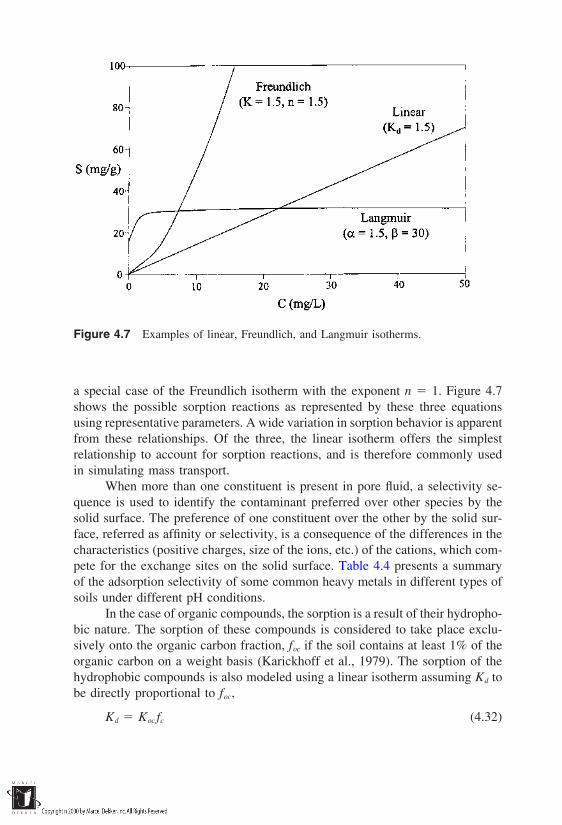
Figure 4.7 Examples of linear, Freundlich, and Langmuir isotherms.

a special case of the Freundlich isotherm with the exponent n 1. Figure 4.7shows the possible sorption reactions as represented by these three equationsusing representative parameters. A wide variation in sorption behavior is apparentfrom these relationships. Of the three, the linear isotherm offers the simplestrelationship to account for sorption reactions, and is therefore commonly usedin simulating mass transport.

When more than one constituent is present in pore fluid, a selectivity se-quence is used to identify the contaminant preferred over other species by thesolid surface. The preference of one constituent over the other by the solid sur-face, referred as affinity or selectivity, is a consequence of the differences in thecharacteristics (positive charges, size of the ions, etc.) of the cations, which com-pete for the exchange sites on the solid surface. Table 4.4 presents a summaryof the adsorption selectivity of some common heavy metals in different types ofsoils under different pH conditions.

In the case of organic compounds, the sorption is a result of their hydropho-bic nature. The sorption of these compounds is considered to take place exclu-sively onto the organic carbon fraction, foc if the soil contains at least 1% of theorganic carbon on a weight basis (Karickhoff et al., 1979). The sorption of thehydrophobic compounds is also modeled using a linear isotherm assuming Kd tobe directly proportional to foc,

Kd Koc fc (4.32)

Table 4.4 Adsorption Selectivity of Heavy Metals in Different Soils

Material Selectivity order References

Kaolinite clay (pH 3.5–6) Pb Ca Cu Mg Zn Cd Farrah and Pickering (1977)Kaolinite clay (pH 5.5–7.5) Cd Zn Ni Puls and Bohn (1988)Illite clay (pH 3.5–6) Pb Cu Zn Ca Cd Mg Farrah and Pickering (1977)Montmorillonite clay Ca Pb Cu Mg Cd Zn Farrah and Pickering (1977)

(pH3.5–6)Montmorillonite clay Cd Zn Ni Puls and Bohn (1988)

(pH5.5–7.5)Al oxides (amorphous) Cu Pb Zn Cd Kinniburgh et al. (1976)Mn oxides Cu Zn Murray (1975)Fe oxides (amorphous) Pb Cu Zn Cd Benjamin and Leckie (1981)Goethite Cu Pb Zn Cd Forbes et al. (1974)Fulvic acid (pH 5.0) Cu Pb Zn Schnitzer and Skinner (1967)Humic acid (pH 4–6) Cu Pb Cd Zn Stevenson (1977)Japanese dominated by vol- Pb Cu Zn Cd Ni Biddappa et al. (1981)

canic parent materialMineral soils (pH 5.0), Pb Cu Zn Cd Elliot et al. (1986)

(with no organics)Mineral soils (containing Pb Cu Cd Zn Elliot et al. (1986)

20–40 g/kg organics)

Source: Yong et al. (1992).

where Koc partition coefficient of a compound between organic carbon andwater (Karickhoff et al., 1979). In several studies, Koc was found to be relatedto Kow, the octanol/water partition coefficient, because of the similarity in theadsorption behavior of organic carbon and octanol. Some regression equationsrelating the two parameters are

Karickhoff et al., 1979 log Koc 0.21 log Kow (4.33)

Kenaga and Goring, 1980 log Koc 1.377 0.544 log Kow (4.34)

SchwarzenbachandWestall,1981 log Koc 0.490.72 log Kow (4.35)

Hassett et al., 1983 log Koc 0.088 0.909 log Kow (4.36)

4.3.2 Equilibrium and Kinetic Models of Reactions

The processes discussed in the preceding section occur at different rates toachieve chemical equilibrium. A simplistic approach would be to assume thatthe reactions would come to equilibrium instantaneously. This is justified in thecase of acid–base reactions and a few others, and is termed the equilibrium modelof reaction. However, in majority of the reactions, the reaction process is transient

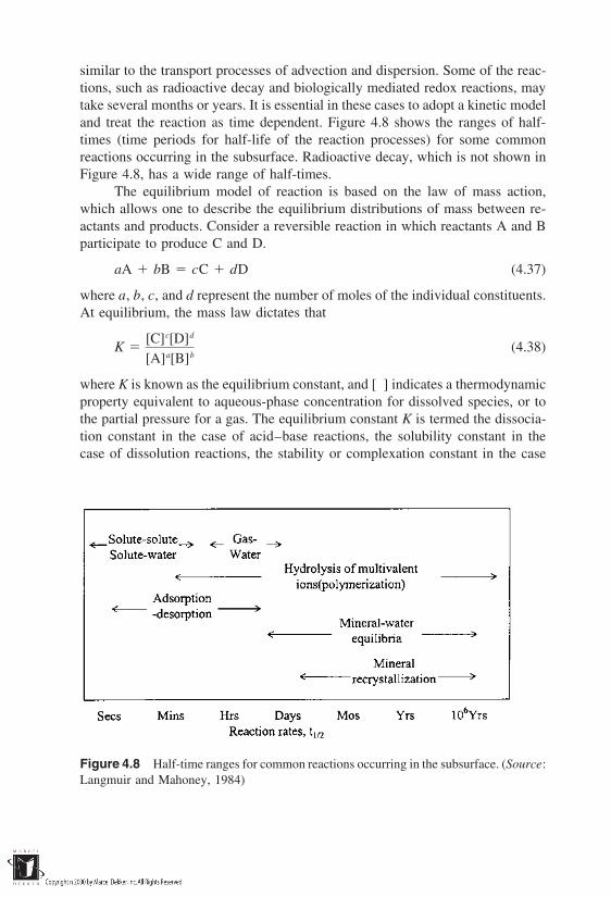
similar to the transport processes of advection and dispersion. Some of the reac-tions, such as radioactive decay and biologically mediated redox reactions, maytake several months or years. It is essential in these cases to adopt a kinetic modeland treat the reaction as time dependent. Figure 4.8 shows the ranges of half-times (time periods for half-life of the reaction processes) for some commonreactions occurring in the subsurface. Radioactive decay, which is not shown inFigure 4.8, has a wide range of half-times.

The equilibrium model of reaction is based on the law of mass action,which allows one to describe the equilibrium distributions of mass between re-actants and products. Consider a reversible reaction in which reactants A and Bparticipate to produce C and D.

aA bB cC dD (4.37)

where a, b, c, and d represent the number of moles of the individual constituents.At equilibrium, the mass law dictates that

K [C]c[D]d

[A]a[B]b(4.38)

where K is known as the equilibrium constant, and [ ] indicates a thermodynamicproperty equivalent to aqueous-phase concentration for dissolved species, or tothe partial pressure for a gas. The equilibrium constant K is termed the dissocia-tion constant in the case of acid–base reactions, the solubility constant in thecase of dissolution reactions, the stability or complexation constant in the case

Figure 4.8 Half-time ranges for common reactions occurring in the subsurface. (Source:Langmuir and Mahoney, 1984)

of complexation reactions, the substitution constant in the case of substitution/hydrolysis, and the adsorption constant for surface reactions. Equation (4.38) isalso used to identify the departure from equilibrium of a given reaction. Forinstance, if the right-hand side (r.h.s.) of Eq. (4.38), also known as the ion activityproduct (IAP), is less than K, the reaction is proceeding forward; and if it isgreater than K, the reaction is proceeding backward, reducing the products andincreasing the reactants.

A kinetic model for the reaction in Eq. (4.37) involves a rate law of theform

rA k1[A]x1[B]x2 k2[C]y1[D]y2 (4.39)

where rA is the rate of mass accumulation of the constituent A, k1 and k2 are therate constants for the forward and reverse reactions, and x1, x2, y1, and y2 areempirical or stoichiometric coefficients and represent the order of the reaction.The first term of the r.h.s. in Eq. (4.39) indicates the rate at which the speciesA is consumed in the forward direction and the second term indicates the rateat which it is produced in the reverse direction. Equation (4.39) yields a sink-source term for a given constituent and can be incorporated directly in the masstransport equation as discussed in the next section. In a number of cases, thereactions can be represented by simplified forms of rate laws such as those givenbelow (Langmuir and Mahoney, 1984),

rC k1[14C] (4.40)

rFe k1[Fe2][O2] (4.41)

where rC and rFe are the rates of mass changes of the irreversible decay of 14Cand that of Fe2 in the following radioactive decay and oxidation reactions:

14C → 14N e (4.42)

Fe2 14

O2 12

H2O → FeOH2 (4.43)

Often, a number of reactions may be proceeding in parallel, making it un-wieldy to express the kinetics of a given constituent in a single equation. Also,when the reactions are of higher order, the solution of mass transport equationstends to be complicated. For these reasons, simplifications are often sought whendescribing geochemical reactions in mass transport phenomena.

The National Research Council (1990) notes that, in general, the equilib-rium models are well established only for oxidation/reduction and acid/base reac-tions. The kinetic models are well established for radioactive reactions, dissolu-tion, complexation, and substitution/hydrolysis; however, the rate constantsneeded for these models are poorly defined for several relevant species in the

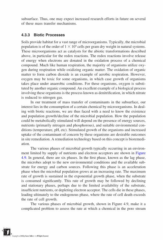
subsurface. Thus, one may expect increased research efforts in future on severalof these mass transfer mechanisms.

4.3.3 Biotic Processes

Soils provide habitat for a vast range of microorganisms. Typically, the microbialpopulation is of the order of 1 106 cells per gram dry weight in natural systems.These microorganisms act as catalysts for the abiotic transformations describedabove, in particular for the redox reactions. The redox reactions involve releaseof energy when electrons are donated in the oxidation process of a chemicalcompound. Much like human respiration, the majority of organisms utilize oxy-gen during respiration while oxidizing organic matter. The oxidation of organicmatter to form carbon dioxide is an example of aerobic respiration. However,oxygen may be toxic for some organisms, in which case growth of organismstakes place under anaerobic conditions. For these organisms, oxygen is substi-tuted by another organic compound. An excellent example of a biological processinvolving these organisms is the process known as denitrification, in which nitrateis reduced to nitrogen gas.

In our treatment of mass transfer of contaminants in the subsurface, ourinterest lies in the consumption of a certain chemical by microorganisms. In deal-ing with biotic reactions, we are thus faced with a need to know the existenceand population growth/decline of the microbial population. How the populationcould be metabolically stimulated will depend on the presence of energy sources,nutrients (primarily nitrogen and phosphorous), and suitable environmental con-ditions (temperature, pH, etc). Stimulated growth of the organisms and increaseduptake of the contaminant of concern by these organisms are desirable outcomesin site remediation. A remediation technology based on this concept is bioremedi-ation.

The various phases of microbial growth typically occurring in an environ-ment limited by supply of nutrients and electron acceptors are shown in Figure4.9. In general, there are six phases. In the first phase, known as the lag phase,the microbes adopt to the new environmental conditions and the available sub-strate for energy and carbon sources. Following this phase is an accelerationphase when the microbial population grows at an increasing rate. The maximumrate of growth is sustained in the exponential growth phase, when the substrateis consumed significantly. This rate of growth may be followed by decliningand stationary phases, perhaps due to the limited availability of the substrate,insufficient nutrients, or depleting electron acceptor. The cells die in these phases,leading ultimately to the endogenous phase, where the rate of cell death exceedsthe rate of cell growth.

The various phases of microbial growth, shown in Figure 4.9, make it acomplicated problem to assess the rate at which a chemical in the pore stream

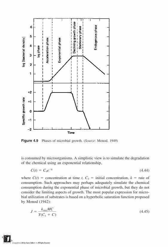
Figure 4.9 Phases of microbial growth. (Source: Monod, 1949)

is consumed by microorganisms. A simplistic view is to simulate the degradationof the chemical using an exponential relationship,

C(t) C0ekt (4.44)

where C(t) concentration at time t, C0 initial concentration, k rate ofconsumption. Such approaches may perhaps adequately simulate the chemicalconsumption during the exponential phase of microbial growth, but they do notconsider the limiting aspects of growth. The most popular expression for micro-bial utilization of substrates is based on a hyperbolic saturation function proposedby Monod (1942):

J kmaxMC

Y(Ck C )(4.45)

where J rate of change in substrate concentration, kmax maximum growthrate of microbes, M microbial mass, C concentration of the growth-limitingsubstrate, Y yield coefficient indicating the organisms formed per substrateutilized, and Ck substrate concentration at which growth rate is kmax/2. As seenin Eq. (4.45), smaller values of Ck and larger values of kmax are associated withmaximum rate of substrate consumption. It is important to note that microbialmass M, is itself not constant, so Eq. (4.45) must be coupled with another equationdescribing the rate of change in M. This is usually accomplished using Monodkinetics with a decay term that accounts for cell death. Thus,

dM

dt kmax MY

C

Ck C bM (4.46)

where b coefficient representing the rate at which microorganisms decay. Theinterdependency between the microbial mass and substrate concentrations hasled to several biodegradation models, most of which use the above principlesbased on Monod kinetics. The biofilm model (McCarty et al., 1984) is one suchmodel which accounts for the processes involved in the transport of substratechemical to the microbes. It conceptualizes that the microorganisms bind to thesurface of the solid matrix in the form of a biofilm, deriving the needed substratefrom the pore liquid (Fig. 4.10). A diffusion layer is identified between the bulk

Figure 4.10 Conceptualization of substrate flux into the biofilm. (Source: McCarty etal., 1984)

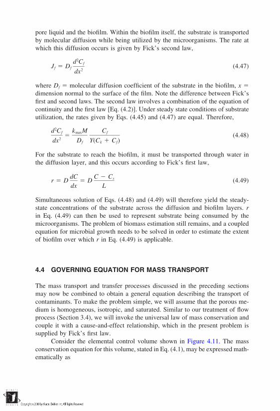
pore liquid and the biofilm. Within the biofilm itself, the substrate is transportedby molecular diffusion while being utilized by the microorganisms. The rate atwhich this diffusion occurs is given by Fick’s second law,

Jf Df

d2Cf

dx2(4.47)

where Df molecular diffusion coefficient of the substrate in the biofilm, x dimension normal to the surface of the film. Note the difference between Fick’sfirst and second laws. The second law involves a combination of the equation ofcontinuity and the first law [Eq. (4.2)]. Under steady state conditions of substrateutilization, the rates given by Eqs. (4.45) and (4.47) are equal. Therefore,

d2Cf

dx2

kmaxM

Df

Cf

Y(Ck Cf)(4.48)

For the substrate to reach the biofilm, it must be transported through water inthe diffusion layer, and this occurs according to Fick’s first law,

r DdC

dx D

C Cs

L(4.49)

Simultaneous solution of Eqs. (4.48) and (4.49) will therefore yield the steady-state concentrations of the substrate across the diffusion and biofilm layers. rin Eq. (4.49) can then be used to represent substrate being consumed by themicroorganisms. The problem of biomass estimation still remains, and a coupledequation for microbial growth needs to be solved in order to estimate the extentof biofilm over which r in Eq. (4.49) is applicable.

4.4 GOVERNING EQUATION FOR MASS TRANSPORT

The mass transport and transfer processes discussed in the preceding sectionsmay now be combined to obtain a general equation describing the transport ofcontaminants. To make the problem simple, we will assume that the porous me-dium is homogeneous, isotropic, and saturated. Similar to our treatment of flowprocess (Section 3.4), we will invoke the universal law of mass conservation andcouple it with a cause-and-effect relationship, which in the present problem issupplied by Fick’s first law.

Consider the elemental control volume shown in Figure 4.11. The massconservation equation for this volume, stated in Eq. (4.1), may be expressed math-ematically as

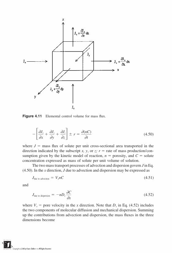
Figure 4.11 Elemental control volume for mass flux.

∂Jx

∂x

∂Jy

∂y

∂Jz

∂z r ∂ (nC)

∂ t(4.50)

where J mass flux of solute per unit cross-sectional area transported in thedirection indicated by the subscript x, y, or z; r rate of mass production/con-sumption given by the kinetic model of reaction, n porosity, and C soluteconcentration expressed as mass of solute per unit volume of solution.

The two mass transport processes of advection and dispersion govern J in Eq.(4.50). In the x direction, J due to advection and dispersion may be expressed as

Jdue to advection VxnC (4.51)

and

Jdue to dispersion nDx∂C

∂x(4.52)

where Vx pore velocity in the x direction. Note that Dx in Eq. (4.52) includesthe two components of molecular diffusion and mechanical dispersion. Summingup the contributions from advection and dispersion, the mass fluxes in the threedimensions become

Jx VxnC nDx∂C

∂x(4.53)

Jy VynC nDy∂C

∂y(4.54)

Jz VznC nDz∂C

∂z(4.55)

Substitution of Eqs. (4.53), (4.54), and (4.55) in (4.50) yields

∂∂x VxnC nDx

∂C

∂x ∂∂y VynC nDy

∂C

∂y ∂

∂z VznC nDz∂C

∂z r ∂(nC )

∂ t

(4.56)

Assuming that the velocities are steady and uniform and that the dispersioncoefficients do not vary in space, Eq. (4.56) may be simplified as

Dx∂ 2C

∂x2 Vx

∂C

∂x Dy∂ 2C

∂y2 Vy

∂C

∂y Dz∂ 2C

∂z2 Vz

∂C

∂z

r

n

∂C

∂ t

(4.57)

It is also assumed in Eq. (4.57) that the porosity of the medium is constant in timeand space. In one dimension, Eq. (4.57) reduces to the well-known advection-dispersion equation (ADE):

Dx∂ 2C

∂x2 Vx

∂C

∂x

r

n

∂C

∂ t(4.58)

The exact form of the ADE depends on the mass transfer processes accountedfor in the term r. Depending on the nature of r, analytical solutions exist for theADE for simple initial and boundary conditions. The following section presentssome common analytical solutions for the ADE.

4.5 SOLUTIONS FOR SPECIAL CASES OF MASSTRANSPORT

We classify the existing analytical solutions for mass transport under three cate-gories:

1. One-dimensional mass transport involving nonreactive constituents,therefore r 0

2. One-dimensional mass transport involving reactive constituents, there-fore one or more of the mass transfer processes should be accountedfor through r

3. Two- and three-dimensional mass transport involving nonreactive andreactive constituents for simple flow conditions

4.5.1 Nonreactive Constituents (r 0)

Pure Diffusion Conditions

Pure diffusion conditions prevail when groundwater velocity, Vx, is so low thatadvective transport process can be ignored. Waste containment barriers such asclay or synthetic liners fall into this category, since they possess low permeabilit-ies and diffusion tends to dominate advection. The ADE [Eq. (4.58)] then reducesto Fick’s second law:

∂C

∂ t Dx

∂ 2C

∂x2(4.59)

Given the following initial and boundary conditions,

C(x, 0) Ci x 0

C(0, t) C0 t 0

C(∞, t) Ci t 0

the solution for Eq. (4.59) may be expressed as

C(x, t) Ci (C0 Ci) erfc x

√4Dxt (4.60)

where ‘‘erfc’’ refers to the complement of the error function, ‘‘erf,’’ which isexpressed in terms of its argument β as

erfc(β ) 1 erf(β ) 1 2√π

β

0eu2 du (4.61)

The error function and its complement are listed in Table 4.5 for positive valuesof β. For the special condition when Ci 0, i.e., the medium is initially free ofthe solute, Eq. (4.60) reduces to

C(x, t) C0 erfc x

√4Dxt (4.62)

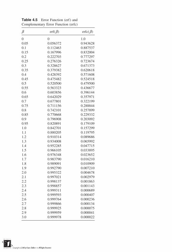
Table 4.5 Error Function (erf) andComplementary Error Function (erfc)

β erf(β) erfc(β)

0 0 1.00.05 0.056372 0.9436280.1 0.112463 0.8875370.15 0.167996 0.8320040.2 0.222703 0.7772970.25 0.276326 0.7236740.3 0.328627 0.6713730.35 0.379382 0.6206180.4 0.428392 0.5716080.45 0.475482 0.5245180.5 0.520500 0.4795000.55 0.563323 0.4366770.6 0.603856 0.3961440.65 0.642029 0.3579710.7 0.677801 0.3221990.75 0.711156 0.2888440.8 0.742101 0.2578990.85 0.770668 0.2293320.9 0.796908 0.2030920.95 0.820891 0.1791091.0 0.842701 0.1572991.1 0.880205 0.1197951.2 0.910314 0.0896861.3 0.934008 0.0659921.4 0.952285 0.0477151.5 0.966105 0.0338951.6 0.976348 0.0236521.7 0.983790 0.0162101.8 0.989091 0.0109091.9 0.992790 0.0072102.0 0.995322 0.0046782.1 0.997021 0.0029792.2 0.998137 0.0018632.3 0.998857 0.0011432.4 0.999311 0.0006892.5 0.999593 0.0004072.6 0.999764 0.0002362.7 0.999866 0.0001342.8 0.999925 0.0000752.9 0.999959 0.0000413.0 0.999978 0.000022

Figure 4.12 Mass transport by molecular diffusion. (Source: Freeze and Cherry, 1979)

Figure 4.12 shows this solution for a range of Dx, typical of nonreactivechemical species in clayey geologic deposits. It is seen that diffusion alone cancause contaminants to travel over distances typical of the thickness of a waste-containment barrier (1–2 m) during typical lifespans of waste-containment struc-tures.

Advection and Dispersion for Continuous Source

For a column initially free of solute and subjected to a continuous source C0 atthe inlet, the initial and boundary conditions may be expressed as

C(x, 0) 0 x 0C(0, t) C0 t 0C(∞, t) 0 t 0

The solution of the ADE under these conditions is given by (Ogata, 1961, 1970)

C

C0

12 erfcx Vxt

2√Dxt expVxx

Dx erfcx Vxt

2√Dxt (4.63)

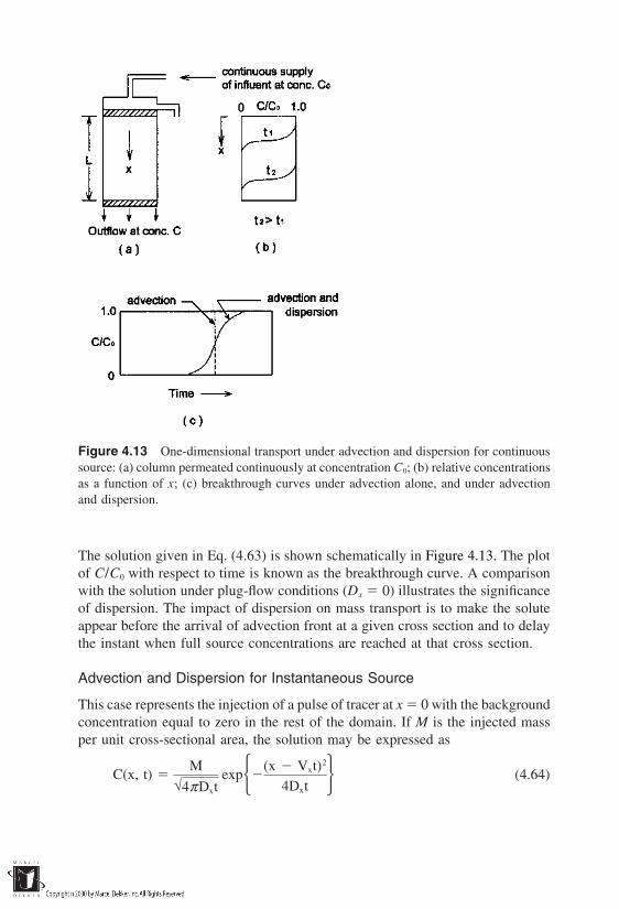
Figure 4.13 One-dimensional transport under advection and dispersion for continuoussource: (a) column permeated continuously at concentration C0; (b) relative concentrationsas a function of x; (c) breakthrough curves under advection alone, and under advectionand dispersion.

The solution given in Eq. (4.63) is shown schematically in Figure 4.13. The plotof C/C0 with respect to time is known as the breakthrough curve. A comparisonwith the solution under plug-flow conditions (Dx 0) illustrates the significanceof dispersion. The impact of dispersion on mass transport is to make the soluteappear before the arrival of advection front at a given cross section and to delaythe instant when full source concentrations are reached at that cross section.

Advection and Dispersion for Instantaneous Source

This case represents the injection of a pulse of tracer at x 0 with the backgroundconcentration equal to zero in the rest of the domain. If M is the injected massper unit cross-sectional area, the solution may be expressed as

C(x, t) M

√4πDxtexp

(x Vxt)2

4Dxt (4.64)

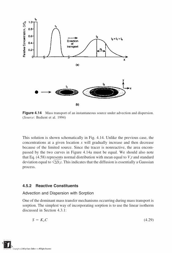
Figure 4.14 Mass transport of an instantaneous source under advection and dispersion.(Source: Bedient et al. 1994)

This solution is shown schematically in Fig. 4.14. Unlike the previous case, theconcentrations at a given location x will gradually increase and then decreasebecause of the limited source. Since the tracer is nonreactive, the area encom-passed by the two curves in Figure 4.14a must be equal. We should also notethat Eq. (4.58) represents normal distribution with mean equal to Vxt and standarddeviation equal to √2Dxt. This indicates that the diffusion is essentially a Gaussianprocess.

4.5.2 Reactive Constituents

Advection and Dispersion with Sorption

One of the dominant mass transfer mechanisms occurring during mass transport issorption. The simplest way of incorporating sorption is to use the linear isothermdiscussed in Section 4.3.1:

S KdC (4.29)

where S quantity of mass sorbed on the surface of solids and Kd distributioncoefficient. The rate expression r is equal to the product of time derivative of Sand dry mass density, ρb. Thus,

r ρb∂S

∂t Kdρb

∂C

∂t(4.65)

Substituting Eq. (4.65) in the ADE [Eq. 4.58)],

Dx∂ 2C

∂x2 Vx

∂C

∂x

ρb

nKd

∂C

∂ t

∂C

∂ t(4.66)

Rearrangement of terms in Eq. (4.66) yields

Dx∂ 2C

∂x2 Vx

∂C

∂x

∂C

∂ t 1 ρbKd

n (4.67)

or, in its familiar form,

Dx

R

∂ 2C

∂x2

Vx

R

∂C

∂x

∂C

∂ t(4.68)

where R (1 ρbKd /n) is known as the retardation factor since it has the effectof retarding the transport of adsorbed species relative to the advection front.Given the initial and boundary conditions,

C(x, t) 0 for t 0 and x 0C(x, t) C0 for x 0C(x, t) 0 for x ∞

the solution of Eq. (4.68) is (Ogata and Banks, 1961, 1970)

C(x, t) C0

2 erfcRx Vxt

2√RDxt expVx x

Dx erfcRx Vxt

2√RDxt (4.69)

Note that Eq. (4.69) reduces to Eq. (4.63) when R 1, i.e., the species is nonreac-tive and Kd 0.

Advection and Dispersion with Sorption and Zero-OrderProduction or Decay

When the reaction process is independent of species concentration, a constantsink/source term γ, can be used for r. Although this is a rare occurrence, it pro-

vides simple approximates in a number of mass transport problems. With a zero-order production term, the ADE becomes

Dx

R

∂ 2C

∂x2

Vx

R

∂C

∂x

γR

∂C

∂ t(4.70)

Analytical solutions for Eq. (4.70) are available for simple initial and boundaryconditions (van Genuchten and Alves, 1982). One solution for a specific set ofinitial and boundary conditions is given here as an example.

For

C(x, 0) Ci,

C(0, t) C0 0 t t0

0 t t0

and

∂C

∂x(∞, t)finite,

C(x, t)Ci (C0 Ci)A(x, t)B(x, t) 0 t t0

Ci (C0 Ci)A(x, t)B(x, t)C0A(x, t t0) t t0(4.71)

where

A(x, t) 12

erfcRx Vxt

2√DxRt 12

expVxx

Dx erfcRx Vxt

2√DxRt and

B(x, t) γR t

(Rx Vxt)2Vx

erfcRx Vxt

2√DxRt

(Rx Vxt)2Vx

expVxx

Dx erfcRx Vxt

2√DxRt Advection and Dispersion with Sorption, Zero-Order Production,and First-Order Decay

Many of the mass transfer processes including radioactive decay, biodegradation,and hydrolysis can be adequately described using first-order kinetics. In thesecases,

r d(nC )

dt λnC (4.72)

where λ is the first-order decay rate [T1]. The ADE of Eq. (4.70) will now become

Dx

R

∂ 2C

∂x2

Vx

R

∂C

∂x

λCR

γR

∂C

∂ t(4.73)

Analytical solutions for Eq. (4.73) are listed in van Genuchten and Alves (1982)for several sets of initial and boundary conditions. For the following set of initialand boundary conditions,

C(x, 0) Ci

C(0, t) C0 0 t t0

0 t t0

∂C

∂x(∞, t) 0

the solution for Eq. (4.73) is

C(x, t)γλ

Ci γλA(x, t)C0

γλB(x, t) 0 t t0

γλ

Ci γλA(x, t)C0

γλB(x, t)C0B(x, t t0) t t0

where

A(x, t) expλ t

R1 12

erfcRx Vx t

2√DxRt

12

expVx x

Dx erfcRx Vxt

2√DxRt B(x, t)

12

exp(Vx U)x2Dx

erfcRx Uxt

2√DxRt

12

exp(Vx U)x2Dx

erfcRx Ut

2√DxRt and

U Vx1 4λRD

Vx2

1/2

(4.74)

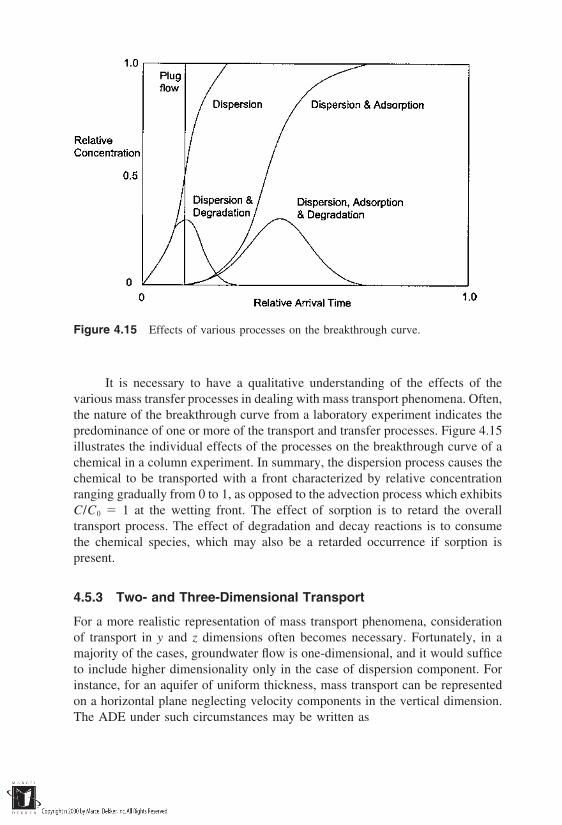
Figure 4.15 Effects of various processes on the breakthrough curve.

It is necessary to have a qualitative understanding of the effects of thevarious mass transfer processes in dealing with mass transport phenomena. Often,the nature of the breakthrough curve from a laboratory experiment indicates thepredominance of one or more of the transport and transfer processes. Figure 4.15illustrates the individual effects of the processes on the breakthrough curve of achemical in a column experiment. In summary, the dispersion process causes thechemical to be transported with a front characterized by relative concentrationranging gradually from 0 to 1, as opposed to the advection process which exhibitsC/C0 1 at the wetting front. The effect of sorption is to retard the overalltransport process. The effect of degradation and decay reactions is to consumethe chemical species, which may also be a retarded occurrence if sorption ispresent.

4.5.3 Two- and Three-Dimensional Transport

For a more realistic representation of mass transport phenomena, considerationof transport in y and z dimensions often becomes necessary. Fortunately, in amajority of the cases, groundwater flow is one-dimensional, and it would sufficeto include higher dimensionality only in the case of dispersion component. Forinstance, for an aquifer of uniform thickness, mass transport can be representedon a horizontal plane neglecting velocity components in the vertical dimension.The ADE under such circumstances may be written as

Dx∂ 2C

∂x2 Dy

∂ 2C

∂y2 Vx∂C

∂x

r

n

∂C

∂ t(4.75)

De Josselin De Jong (1958) provided a solution for the mass transport ina two-dimensional field for the specific case of pulse injection over a finite linesource, such as a well point, into a horizontal flow field. For a pulse tracer withinitial concentration C0 injected at a point (x0, y0) in the horizontal field, thesolution was given as

C(x, y, t) C0 A

4π t(DxDy)1/2exp

[(x x0) Vxt]2

4Dxt

(y y0)2

4Dyt (4.76)

where A area over which the pulse is injected. This solution can be extendedto include dispersion component in the z dimension (Baetsle, 1969). For a sourcewith an initial concentration of C0 and volume V0, its spread in space and timecoordinates was given as

C(x, y, z, t) C0V0

8(π t)3/2(DxDyDz)1/2

exp(x Vxt)2

4Dxt

y2

4Dyt

z2

4Dzt λt

(4.77)

As seen in Eq. (4.77), first-order decay of the species (represented by the decayconstant λ) was accounted for in this solution. A close examination of Eq. (4.77)indicates that the source progresses as a Gaussian plume with its center at x Vxt, y 0, z 0, and the standard deviations in the three dimensions equalto

σx √2Dxt (4.78a)

σy √2Dyt (4.78b)

σz √2Dzt (4.78c)

The concentration of the species is always maximum at the center of the plume,and is given by

Cmax C(Vxt, 0, 0) C0V0eλt

8(π t)3/2(DxDyDz)1/2(4.79)

Wilson and Miller (1978) provided another set of analytical solutions formass transport in two dimensions, accounting for the processes of advection inthe x dimension (the direction of flow), dispersion in the x and y dimensions,

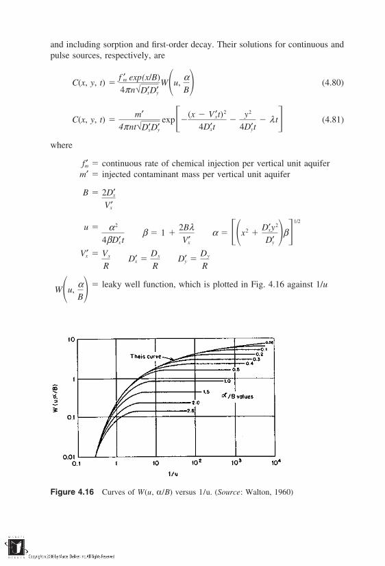
and including sorption and first-order decay. Their solutions for continuous andpulse sources, respectively, are

C(x, y, t) f ′m exp(x/B)4πn√D′xD′y

Wu,αB (4.80)

C(x, y, t) m′

4πnt√D′xD′yexp

(x V ′xt)2

4D′xt

y2

4D′yt λ t (4.81)

where

f ′m continuous rate of chemical injection per vertical unit aquiferm′ injected contaminant mass per vertical unit aquifer

B 2D′xV′x

u α 2

4βD′x tβ 1

2BλV′x

α x2 D′xy2

D′y β1/2

V′x Vx

RD′x

Dx

RD′y

Dy

R

leaky well function, which is plotted in Fig. 4.16 against 1/uWu,

αB

Figure 4.16 Curves of W(u, α/B) versus 1/u. (Source: Walton, 1960)

We note that analytical solutions for mass transport equation are possibleonly for simple initial and boundary conditions. They are suitable for specializedcases where the velocity is steady and the porous medium is homogeneous andisotropic in its hydrogeological parameters. These limitations often restrict theuse of the simple solutions presented above. One would then resort to numericalsolutions, which implement finite-difference or finite-element methods. A num-ber of software packages are available for the purpose of studying mass transportin porous media, and the next section provides a brief summary of the capabilitiesof these packages.

4.6 SURVEY OF COMPUTER SOFTWARE FOR MASSTRANSPORT AND TRANSFER MODELING

The Groundwater Quality Technical Committee of the Environmental Engi-neering Division of the ASCE (American Society of Civil Engineers) launcheda group of activities in 1991 in an attempt to summarize the state of the art ofcontaminated-groundwater modeling practice and to provide guidelines for modelusers. Based on a survey conducted by the committee as well as by other agenciesincluding the U.S. Environmental Protection Agency (EPA), Geraghty andMiller, and Brookhaven National Laboratory, it was reported that a total of about54 different models were used by state agencies and consultants. The most fre-quently used models simulating mass transport phenomena included (AmericanSociety of Civil Engineers, 1996), in alphabetical order, are:

1. CFEST 7. RANDOMWALK2. DYNTRACK 8. RESSQ3. MIGRATE 9. RITZ4. MOC 10. SOLUTE5. MT3D 11. SUTRA6. POLLUTE

Table 4.6 lists the common practical applications of these models. In gen-eral, the popular applications are (1) to estimate contaminant plume migration,and (2) to determine sensitivity of contaminant migration to various hydrogeolog-ical and source parameters. The various transport processes simulated by thesemodels are listed in Table 4.7. The models essentially solve the advection-disper-sion equation in one form or another, using either analytical, semianalytical (po-tential theory, finite-layer technique), or numerical (finite-difference, finite-ele-ment) methods. All of the models are capable of simulating mass transport dueto advection and molecular diffusion, and only RITZ does not simulate transportdue to hydrodynamic dispersion. RITZ was a model developed to investigateland treatment alternatives in the disposal of oil sludges, primarily originating

Table 4.6 Practical Applications of Frequently Used Transport Models

Applications Models

Estimate contaminant plume migration plume Allmigration.

Determine sensitivity of migration to various Allparameters.

Assess leachate collection systems below waste MIGRATE, POLLUTEsites.

Design barriers in a landfill. MIGRATE, POLLUTESimulate pollutant transport through clayey MIGRATE, POLLUTE

soils.Locate landfill, hazardous waste, and nuclear CFEST, MOC, MT3D, RNDWALK,

waste sites. SUTRA DYNTRACK, RESSQHelp calibrate flow model. CFEST, MOC, MT3D, RNDWALK,

SUTRA DYNTRACK, RESSQInvestigate contaminant source distribution and CFEST, MOC, MT3D, RNDWALK,

loading history: SUTRA DYNTRACK, RESSQInvestigate remedial action alternatives (inter- CFEST, MOC, MT3D RNDWALK

ceptor drains and withdrawal/injection wells) DYNTRACK, RESSQfor cleanup or containment of contaminatedwater

Simulate saltwater intrusion. CFEST, SUTRASimulate energy transport. CFEST, SUTRALand treatment and cleanup criteria of petro- RITZ

leum refinery wastes.Analytical solutions to several practical prob- POLLUTE

lems.Stimulate multiphase flow. RITZ

Source: American Society of Civil Engineers (1996).

from petroleum refinery wastes, and is the only model that can simulate multi-phase flow (the next chapter is devoted to issues of multiphase flow). All of themodels except RITZ can simulate the effects of radioactive decay, and onlyCFEST, MOC, and SOLUTE do not simulate the effects of chemical biodegrad-ability. Sorption process is simulated in all the models through a user-definedretardation factor; however, most of the models can also simulate sorption and/or other chemical reactions indirectly, using parameters such as bulk density,organic carbon content, solubility, sorption constant, cation-exchange capacity,reaction rate constants, and partition coefficient.

The various categories of input parameters for these models were identifiedas follows:

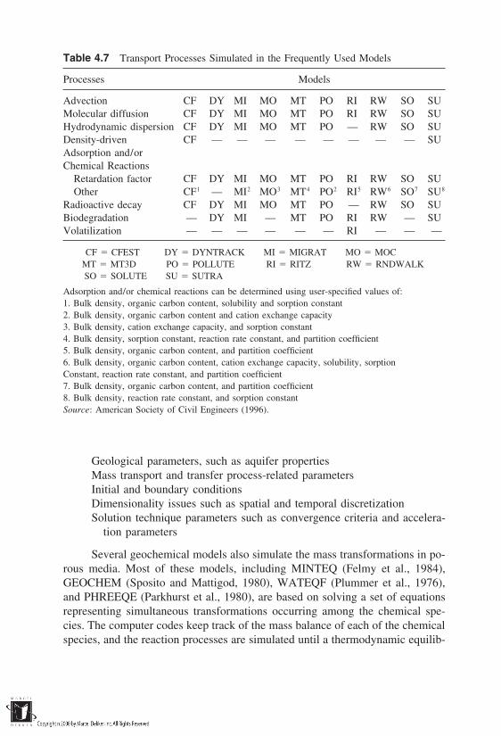
Table 4.7 Transport Processes Simulated in the Frequently Used Models

Processes Models

Advection CF DY MI MO MT PO RI RW SO SUMolecular diffusion CF DY MI MO MT PO RI RW SO SUHydrodynamic dispersion CF DY MI MO MT PO — RW SO SUDensity-driven CF — — — — — — — — SUAdsorption and/orChemical Reactions

Retardation factor CF DY MI MO MT PO RI RW SO SUOther CF1 — MI2 MO3 MT4 PO2 RI5 RW6 SO7 SU8

Radioactive decay CF DY MI MO MT PO — RW SO SUBiodegradation — DY MI — MT PO RI RW — SUVolatilization — — — — — — RI — — —

CF CFEST DY DYNTRACK MI MIGRAT MO MOCMT MT3D PO POLLUTE RI RITZ RW RNDWALKSO SOLUTE SU SUTRA

Adsorption and/or chemical reactions can be determined using user-specified values of:1. Bulk density, organic carbon content, solubility and sorption constant2. Bulk density, organic carbon content and cation exchange capacity3. Bulk density, cation exchange capacity, and sorption constant4. Bulk density, sorption constant, reaction rate constant, and partition coefficient5. Bulk density, organic carbon content, and partition coefficient6. Bulk density, organic carbon content, cation exchange capacity, solubility, sorptionConstant, reaction rate constant, and partition coefficient7. Bulk density, organic carbon content, and partition coefficient8. Bulk density, reaction rate constant, and sorption constantSource: American Society of Civil Engineers (1996).

Geological parameters, such as aquifer propertiesMass transport and transfer process-related parametersInitial and boundary conditionsDimensionality issues such as spatial and temporal discretizationSolution technique parameters such as convergence criteria and accelera-

tion parameters

Several geochemical models also simulate the mass transformations in po-rous media. Most of these models, including MINTEQ (Felmy et al., 1984),GEOCHEM (Sposito and Mattigod, 1980), WATEQF (Plummer et al., 1976),and PHREEQE (Parkhurst et al., 1980), are based on solving a set of equationsrepresenting simultaneous transformations occurring among the chemical spe-cies. The computer codes keep track of the mass balance of each of the chemicalspecies, and the reaction processes are simulated until a thermodynamic equilib-

rium is achieved. Most codes at present, however, consider only equilibrium mod-els of reactions, which precludes their applicability to field scenarios where akinetic reaction model might be more appropriate.

REFERENCES

American Society of Civil Engineers. (1996). Quality of Ground Water, Guidelines forSelection and Application of Frequently Used Models, ASCE Manuals and Reportson Engineering Practice No. 85. ASCE, New York.

Baetsle, L. H. (1969). Migration of radionuclides in porous media. In A. M. F. Duhamel(ed.), Progress in Nuclear Energy Series XII, Health Physics, pp. 707–730. Perga-mon Press, Elmsford, NY.

Bedient, P. B., Rifai, H. S., and Newell, C. J. (1994). Ground Water Contamination, Trans-port and Remediation. Prentice-Hall, Englewood Cliffs, NJ.

Benjamin, M. M., and Leckie, J. O. (1981). Multiple-site adsorption of Cd, Zn, and Pbon amorphous iron oxyhydroxide. J. Colloid Interface Sci., 79:209–221.

Biddappa, C. C., Chino, M., and Kumazawa, K. (1981). Adsorption, desorption, potentialand selective distribution of heavy metals in selected soils of Japan. J. Environ.Sci. Health B, 156:511–528.

Chiou, C. T., Schmedding, D. W., and Manes, M. (1982). Partitioning of organic com-pounds in octanol-water systems. Environ. Sci. Technol., 16:4–10.

De Josselin De Jong, G. (1958). Longitudinal and transverse diffusion in granular deposits.Trans. Am. Geophys. Union, 39(1):67.

Domenico, P. A., and Schwartz, F. W. (1990). Physical and Chemical Hydrogeology.Wiley, New York.

Elliott, H. A., Liberati, M. R., and Huang, C. P. (1986). Competitive adsorption of heavymetals by soils. J. Environ. Qual., 15:214–219.

Farrah, H., and Pickering, W. F. (1977). The sorption of lead and cadmium species byclay minerals. Austral. J. Chem., 30:1417–1422.

Felmy, A. R., Brown, S. M., Onishi, Y., Yabusaki, S. B., Argo, R. S., Girvin, D. C., andJenne, E. A. (1984). Modeling the transport, speciation, and fate of heavy metals inaquatic systems, EPA Project Summary, EPA-600/53-84-033. U.S. EnvironmentalProtection Agency, Athens, GA.

Forbes, E. A., Posner, A. M., and Quirk, J. P. (1974). The specific adsorption of inorganicHg (II) species and Co (II) complex ions on geothite. J. Colloid Interface Sci., 49:403–409.

Freeze, R. A., and Cherry, J. A. (1979). Groundwater. Prentice-Hall, Englewood Cliffs,NJ.

Hassett, J. J., Banwart, W. L., and Griffin, R. A. (1983). Correlation of compound proper-ties with sorption characteristics of nonpolar compounds by soils and sediments:Concepts and limitations. In C. W. Francis an S. I. Auerbach (eds.), Environmentand Solid Wastes: Characterization, Treatment and Disposal, pp. 161–178. Butter-worth, Stoneham, MA.

Johnson, R. L., Palmer, C. D., and Fish, W. (1989). Subsurface chemical processes. In

Transport and Fate of Contaminants in the Subsurface, EPA/625/4-89/019, pp. 41–56. U.S. Environmental Protection Agency, Cincinnati, OH, and Ada, OK.

Karickhoff, S. W., Brown, D. S., and Scott, T. A. (1979). Sorption of hydrophobic pollut-ants on natural sediments. Water Res., 13:241–248.

Kenaga, E. E., and Goring, C. A. I. (1980). ASTM Special Technical Publication 707.American Society for Testing Materials, Washington, DC.

Kinniburgh, D. G., Jackson, M. L., and Syers, J. K. (1976). Adsorption of alkaline earth,transition and heavy metal cations by hydrous oxide gels of iron and aluminum.Soil Sci. Soc. Am. J., 40:796–799.

Langmuir, D., and Mahoney, J. (1984). Chemical equilibrium and kinetics of geochemicalprocesses in groundwater studies. In B. Hitchon and E. I. Walliek (eds.) Proceed-ings of the First Canadian/American Conference on Hydrogeology, pp. 69–95.National Water Well Association, Dublin, OH.

Lerman, A. (1979). Geochemical processes—Water and sediment environments. Wiley,New York.

Li, Y-H., and Gregory, S. (1974). Diffusion of ions in sea water and in deep-sea sediments.Geochim. Cosmochim. Acta, 38(5):703–714.

Mackay, D. M., and Leinonen, P. J. (1975). Rate of evaporation of low-solubility contami-nants from water bodies to atmosphere. Environ. Sci. Technol., 9(8):1178–1180.

McCarty, P. L., Rittman, B. E., and Bouwer, E. J. (1984). Microbiological processes affect-ing chemical transformations in groundwater. In G. Bitton and C. P. Gerba (eds.),Groundwater Pollution Microbiology, pp. 89–115. Wiley, New York.

Monod, J. (1942) Recherches sur la croissance des cultures bacteriennes. Herman & Cie,Paris.

Monod, J. (1949). The growth of bacterial cultures. Ann. Rev. Microbiol. 3:371.Montgomery, J. H. (1991). Groundwater Chemicals Desk Reference, Vol. 2. Lewis Pub-

lishers, Chelsea, MI.Montgomery, J. H. and Welkom, L. M. (1990). Groundwater Chemicals Desk Reference.

Lewis Publishers, Chelsea, MI.Morel, F. M. M. (1983). Principles of Aquatic Chemistry. J Wiley, New York.Murray, J. W. (1975). The interaction of metal ions at the manganese dioxide solution

interface. Geochim. Cosmochim. Acta, 39:505–519.National Research Council. (1990). Ground Water Models: Scientific and Regulatory Ap-

plications. National Academy Press, Washington, DC.Neely, W. B. (1985). Hydrolysis. In W. B. Neely and G. E. Blau (eds.), Environmental

Exposure from Chemicals, Vol. I, pp. 157–173. CRC Press, Boca Raton, FL.Nye, P. H. (1979). Diffusion of ions and uncharged solutes in soils and soil clays. Adv.

Agron. 31:25–272.Ogata, A. (1970). Theory of dispersion in a granular medium. U.S. Geol. Surv. Prof. Paper

411–I.Ogata, A., and Banks, R. B. (1961). A solution of the differential equation of longitudinal

dispersion in porous media. U.S. Geol. Surv. Prof. Paper 411–A.Olsen, S. R., Kemper, W. D., and van Schaik, J. C. (1965). Self-diffusion coefficients of

phosphorous in soil measured by transient and steady-state methods. Proc. Soil Sci.Soc. Am., 29(2):154–158.

Parkhurst, D. L., Thorstenson, D. C., and Plummer, L. N. (1980). PHREEQE—A com-

puter program for geochemical calculations. U.S. Geol. Surv. Water Resources In-vestigation 80–96.

Perkins, T. K., and Johnston, O. C. (1963). A review of diffusion and dispersion in porousmedia. Soc. Petroleum Eng. J., 3:70–84.

Plummer, L. N., Jones, B. F., and Truesdell, A. H. (1976). WATEQF—A Fortran IVversion of WATEQ, a computer code for calculating chemical equilibria of naturalwaters. U.S. Geol. Surv. Water Resources Investigation 76–13.

Puls, R. W., and Bohn, H. L. (1988). Sorption of cadmium, nickel, and zinc by kaoliniteand montmorillonite suspensions. Soil Sci. Soc. Am. J., 52:1289–1292.

Quigley, R. M., Yanful, E. K., and Fernandez, F. (1987). Ion transfer by diffusion throughclayey barriers. In R. Woods (ed.), Geotechnical Practice for Waste Disposal, pp.137–158. Geotechnical Special Publication No. 13.

Schnitzer, M., and Skinner, S. I. M. (1967). Organio-metallic interaction in soils: 7. Stabil-ity constants of Pb-, Ni-, Co- and Mg-fluvic acid complexes. Soil Sci.,103:247–252.

Schwarzenbach, R. P., and Westall, J. (1981). Transport of nonpolar organic compoundsrom surface water to groundwater. Laboratory studies. Environ. Sci. Technol., 15:1300–1367.

Shackelford, C. D., and Daniel, D. E. (1991a). Diffusion in saturated soil. I: Background.ASCE J. Geotech. Eng., 117(3):467–484.

Shackelford, C. D., and Daniel, D. E. (1991b). Diffusion in saturated soil. II: Results forcompacted clay. ASCE J. Geotech. Eng., 117(3):485–506.

Sposito, G., and Mattigod, S. V. (1980). GEOCHEM: A computer program for the calcula-tion of chemical equilibria in soil solutions and other natural water systems. Depart-ment of Soils and Environment Report, University of California, Riverside.

Stevenson, F. J. (1975). Stability constants of Cu2, Pb2, and Cd2 complexes with humicacids. Soil Sci. Soc. Am. Proc., 40:665–672.

Stumm, W. and Morgan, J. J. (1981). Aquatic Chemistry, 2nd ed. Wiley, New York.van Genuchten, M. T., and Alves, W. J. (1982). Analytical solutions of the one-dimen-

sional convective-dispersive solute transport equation. U.S. Department of Agricul-ture Technical Bulletin No. 1661. Agricultural Research Service, Washington, DC.

Walton, W. C. (1960). Leaky artesian aquifer conditions in Illinois. Illinois State WaterSurv. Rept. Invest. 39.

Weber, W. J., Jr. (1972). Physicochemical Processes for Water Quality Control. Wiley,New York.

Wilson, J.L., and Miller P. J. (1978). Two-dimensional plume in uniform groundwaterflow. ASCE J. Hydraulics Div., 104:503–514.

Yong, R. N., Mohamed, A. M. O., and Warkentin, B. P. (1992). Principles of ContaminantTransport in Soils. Developments in Geotechnical Engineering 73. Elsevier, Am-sterdam.

5Nonaqueous-Phase Liquids in Soils

5.1 INTRODUCTION

Nonaqueous-phase liquid (NAPL) is a term used to denote any liquid which isimmiscible with water. In geoenvironmental engineering, this term is usuallyassociated with petroleum hydrocarbons such as those leaking from undergroundoil storage tanks or accidental spills of organic chemicals. By virtue of the immis-cibility, an interface or a physical dividing surface between the two bulk liquidsexists in the pore spaces of soils saturated with water and NAPL. In the case ofunsaturated soils, the presence of air creates additional interfaces. In spite of theirimmiscible nature, NAPLs do dissolve in water, and mass transfer occurs acrossthese interfaces. Although this dissolution is rather slow and is not extensive inmost cases, even slight amounts of dissolved NAPLs in potable water suppliesmay result in detrimental health effects. The slow dissolution also causes a long-term source of subsurface contamination. Hence the need to study the fate andtransport of NAPLs in the subsurface.

It is customary to divide the vast range of NAPLs commonly encounteredin geoenvironmental engineering into two general categories, light nonaqueous-phase liquids (LNAPLs) and dense nonaqueous-phase liquids (DNAPLs). Thiscategorization is based on their specific gravity. LNAPLs have a specific gravityless than water, and DNAPLs have a specific gravity greater than water. Tables5.1 and 5.2 list common types of LNAPLs and DNAPLs, respectively, alongwith some of their properties, which will be referred in subsequent sections. Aswe will see in a later section, the difference in density of a NAPL with respectto water governs some important aspects of its transport in the subsurface. There-fore, it is useful to recognize this categorization at the outset.

Throughout this chapter, it will benefit the reader to keep in mind that manyof the principles involved in NAPL transport and entrapment in soils are similar

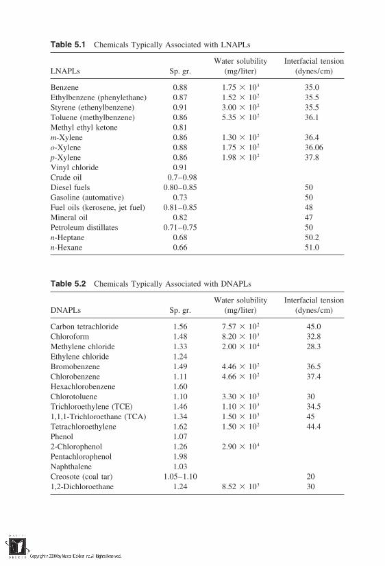
Table 5.1 Chemicals Typically Associated with LNAPLs

Water solubility Interfacial tensionLNAPLs Sp. gr. (mg/liter) (dynes/cm)

Benzene 0.88 1.75 103 35.0Ethylbenzene (phenylethane) 0.87 1.52 102 35.5Styrene (ethenylbenzene) 0.91 3.00 102 35.5Toluene (methylbenzene) 0.86 5.35 102 36.1Methyl ethyl ketone 0.81m-Xylene 0.86 1.30 102 36.4o-Xylene 0.88 1.75 102 36.06p-Xylene 0.86 1.98 102 37.8Vinyl chloride 0.91Crude oil 0.7–0.98Diesel fuels 0.80–0.85 50Gasoline (automative) 0.73 50Fuel oils (kerosene, jet fuel) 0.81–0.85 48Mineral oil 0.82 47Petroleum distillates 0.71–0.75 50n-Heptane 0.68 50.2n-Hexane 0.66 51.0

Table 5.2 Chemicals Typically Associated with DNAPLs

Water solubility Interfacial tensionDNAPLs Sp. gr. (mg/liter) (dynes/cm)

Carbon tetrachloride 1.56 7.57 102 45.0Chloroform 1.48 8.20 103 32.8Methylene chloride 1.33 2.00 104 28.3Ethylene chloride 1.24Bromobenzene 1.49 4.46 102 36.5Chlorobenzene 1.11 4.66 102 37.4Hexachlorobenzene 1.60Chlorotoluene 1.10 3.30 103 30Trichloroethylene (TCE) 1.46 1.10 103 34.51,1,1-Trichloroethane (TCA) 1.34 1.50 103 45Tetrachloroethylene 1.62 1.50 102 44.4Phenol 1.072-Chlorophenol 1.26 2.90 104

Pentachlorophenol 1.98Naphthalene 1.03Creosote (coal tar) 1.05–1.10 201,2-Dichloroethane 1.24 8.52 103 30

to those treated in unsaturated flow (Section 3.6). In an unsaturated soil, theexistence and transport of air phase is in competition with that of water. In awater-saturated soil penetrated by NAPLs, the NAPLs behave similar to air intheir attempt to compete for pore space in the soil. Extending this further to awater-saturated soil penetrated by air and NAPL, all of the three phases competefor the pore space. The relative quantities of the three phases in soil at equilibriumare governed by the same capillarity principle which controls the behavior ofunsaturated soil.

We will look first at the principles of NAPL entrapment in soils at a porescale and then expand our study to a field scale. These principles will lead us to aconceptual understanding of the mass transport and transfer processes of NAPLs.Quantitative modeling of the fate and transport of NAPLs is still at an early stageof development, and is beyond the scope of this book. Our objective in this chap-ter is to gain a qualitative understanding of the mass transport and transfer charac-teristics pertinent to NAPL-penetrated soils.

5.2 PRINCIPLES OF NAPL ENTRAPMENT IN SOILS

Fate and transport of NAPLs in the subsurface depends to a large extent on thequantities of entrapment in the soil pore space. The relative competition amongthe three phases, i.e., water, air, and NAPLs, to occupy the pore space can beunderstood in terms of

1. Interfacial tension between these phases2. Wettability of soils with these phases3. Capillarity principle

In the following sections, we will treat these individually, for a conceptual under-standing of the NAPL entrapment first at a pore scale and then at field scale.

5.2.1 Interfacial Tension

Homogeneous fluids contain molecules bound by van der Waals attractive forces.The magnitudes of these forces differ from fluid to fluid. When two immisciblefluids are brought together, there exists an interface which divides the two setsof molecules (Fig. 5.1). To maintain the force equilibrium, the interface is pulledby the fluid whose molecules are bound by greater attractive forces. Thus, eithera convex or a concave meniscus is formed. The stretched interface behaves muchlike an elastic membrane subjected to tension. The tension existing at the inter-face, known as interfacial tension σ, is a result of the internal pressure difference

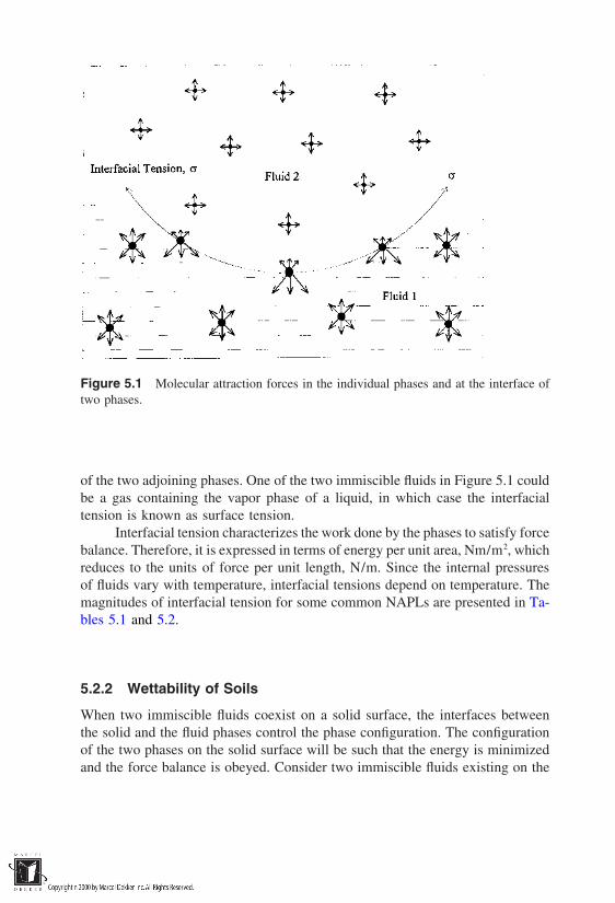
Figure 5.1 Molecular attraction forces in the individual phases and at the interface oftwo phases.

of the two adjoining phases. One of the two immiscible fluids in Figure 5.1 couldbe a gas containing the vapor phase of a liquid, in which case the interfacialtension is known as surface tension.

Interfacial tension characterizes the work done by the phases to satisfy forcebalance. Therefore, it is expressed in terms of energy per unit area, Nm/m2, whichreduces to the units of force per unit length, N/m. Since the internal pressuresof fluids vary with temperature, interfacial tensions depend on temperature. Themagnitudes of interfacial tension for some common NAPLs are presented in Ta-bles 5.1 and 5.2.

5.2.2 Wettability of Soils

When two immiscible fluids coexist on a solid surface, the interfaces betweenthe solid and the fluid phases control the phase configuration. The configurationof the two phases on the solid surface will be such that the energy is minimizedand the force balance is obeyed. Consider two immiscible fluids existing on the

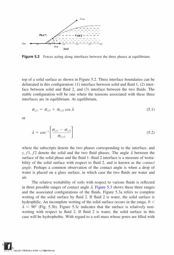
Figure 5.2 Forces acting along interfaces between the three phases at equilibrium.

top of a solid surface as shown in Figure 5.2. Three interface boundaries can bedelineated in this configuration: (1) interface between solid and fluid 1, (2) inter-face between solid and fluid 2, and (3) interface between the two fluids. Thestable configuration will be one where the tensions associated with these threeinterfaces are in equilibrium. At equilibrium,

σs,f1 σs,f2 σ f1,f2 cos λ (5.1)

or

λ cos1 σs,f1 σs,f 2

σ f1, f 2 (5.2)

where the subscripts denote the two phases corresponding to the interface, ands, f 1, f 2 denote the solid and the two fluid phases. The angle λ between thesurface of the solid phase and the fluid 1–fluid 2 interface is a measure of wetta-bility of the solid surface with respect to fluid 2, and is known as the contactangle. Perhaps a common observation of the contact angle is when a drop ofwater is placed on a glass surface, in which case the two fluids are water andair.

The relative wettability of soils with respect to various fluids is reflectedin three possible ranges of contact angle λ. Figure 5.3 shows these three rangesand the associated configurations of the fluids. Figure 5.3a refers to completewetting of the solid surface by fluid 2. If fluid 2 is water, the solid surface ishydrophilic. An incomplete wetting of the solid surface occurs in the range, 0 λ 90° (Fig. 5.3b). Figure 5.3c indicates that the surface is relatively non-wetting with respect to fluid 2. If fluid 2 is water, the solid surface in thiscase will be hydrophobic. With regard to a soil mass whose pores are filled with

Figure 5.3 Possible contact angles between fluids and solid surfaces.

two fluids 1 and 2, the angle λ therefore dictates which fluid coats the solidparticles.

Generally, a porous medium with NAPL and water as fluids 1 and 2 isconsidered to be water-wet if λ (between water and the solids) 70°, NAPL-wet if λ 110°, and neutral if λ is between 70° and 110° (Anderson, 1986). Inmost cases with NAPL and water, the porous medium is commonly treated aswater-wet. In an unsaturated medium where NAPL and air are present, the me-dium is treated as NAPL-wet.

It is important to note that the contact angle may not be definable micro-scopically. The solid surfaces in a soil mass may exhibit tremendous heterogene-ity in their surface characteristics. The surfaces of solid particles may belong toeither silica or clay minerals, which may in turn be coated with iron oxides ormacromolecules of soil humus. Considering this heterogeneity, it may be possibleto define only a composite value for the contact angle. Also, the contact anglemay not be unique for a given surface since it is known to manifest hysteresis,i.e., it depends on the movement of the fluid phase wetting the surface. When adrop of fluid 2 moves along a solid surface (Fig. 5.4), the contact angle λ1 at thereceding end is in general less than the contact angle λ 2 at the proceeding end ofthe drop. This is the primary reason for hysteresis behavior in soil–water retentiondiscussed in Section 3.6. The hysteretic behavior of contact angle can be observedby pushing and pulling a capillary tube in a liquid. The meniscii observed in thetwo stages will exhibit different contact angles.

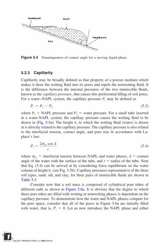
Figure 5.4 Nonuniqueness of contact angle for a moving liquid phase.

5.2.3 Capillarity

Capillarity may be broadly defined as that property of a porous medium whichmakes it draw the wetting fluid into its pores and repels the nonwetting fluid. Itis the difference between the internal pressures of the two immiscible fluids,known as the capillary pressure, that causes this preferential filling of soil pores.For a water–NAPL system, the capillary pressure Pc may be defined as

Pc Pn Pw (5.3)

where Pn NAPL pressure and Pw water pressure. For a small tube insertedin a water-NAPL system, the capillary pressure causes the wetting fluid to bedrawn in (Fig. 5.5a). The height hc to which the wetting fluid (water) is drawnin is directly related to the capillary pressure. The capillary pressure is also relatedto the interfacial tension, contact angle, and pore size in accordance with La-place’s law:

Pc 2σnw cos λ

r(5.4)

where σnw interfacial tension between NAPL and water phases, λ contactangle of the water with the surface of the tube, and r radius of the tube. Notethat Eq. (5.4) can be arrived at by considering force equilibrium on the watercolumn of height hc (see Fig. 5.5b). Capillary pressures representative of the threesoil types, sand, silt, and clay, for three pairs of immiscible fluids are shown inTable 5.3.

Consider now that a soil mass is comprised of cylindrical pore tubes ofdifferent radii as shown in Figure 5.6a. It is obvious that the degree to whichthese pore tubes are filled with wetting or nonwetting phases is dependent on thecapillary pressure. To demonstrate how the water and NAPL phases compete forthe pore space, consider that all of the pores in Figure 5.6a are initially filledwith water, that is, Pc 0. Let us now introduce the NAPL phase and either

Figure 5.5 Capillary pressure in a soil–NAPL system. (Modified from Luckner andSchestakow, 1991).

Table 5.3 Range of Capillary Pressures for Sands, Silts, and Clays

Pore radius, Air/water, Oil/water, Air/oil,r (in m) Pc (in kPa) Pc (in kPa) Pc (in kPa)

Sands 104–105 1.4–14 0.6–6 0.7–7Silts 105–106 14–140 6–60 7–70Clays 106–107 140–1400 60–600 70–700

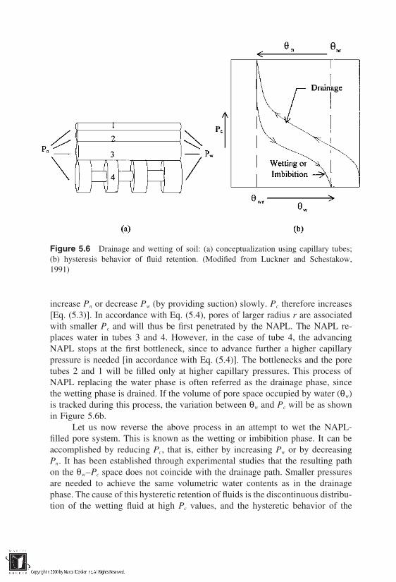
Figure 5.6 Drainage and wetting of soil: (a) conceptualization using capillary tubes;(b) hysteresis behavior of fluid retention. (Modified from Luckner and Schestakow,1991)

increase Pn or decrease Pw (by providing suction) slowly. Pc therefore increases[Eq. (5.3)]. In accordance with Eq. (5.4), pores of larger radius r are associatedwith smaller Pc and will thus be first penetrated by the NAPL. The NAPL re-places water in tubes 3 and 4. However, in the case of tube 4, the advancingNAPL stops at the first bottleneck, since to advance further a higher capillarypressure is needed [in accordance with Eq. (5.4)]. The bottlenecks and the poretubes 2 and 1 will be filled only at higher capillary pressures. This process ofNAPL replacing the water phase is often referred as the drainage phase, sincethe wetting phase is drained. If the volume of pore space occupied by water (θw)is tracked during this process, the variation between θw and Pc will be as shownin Figure 5.6b.

Let us now reverse the above process in an attempt to wet the NAPL-filled pore system. This is known as the wetting or imbibition phase. It can beaccomplished by reducing Pc, that is, either by increasing Pw or by decreasingPn. It has been established through experimental studies that the resulting pathon the θw–Pc space does not coincide with the drainage path. Smaller pressuresare needed to achieve the same volumetric water contents as in the drainagephase. The cause of this hysteretic retention of fluids is the discontinuous distribu-tion of the wetting fluid at high Pc values, and the hysteretic behavior of the

contact angle of the wetting fluid. It is seen from Figure 5.6b that the wettingfluid cannot be drained completely, and a residual water content, θwr, remainseven as Pc approaches infinity. Similarly, during the imbibition phase the nonwet-ting fluid cannot be displaced completely even when Pc 0. The residual contentof the NAPLs that remains during the wetting or imbibition phase is of particularimportance in remediation operations. It is usually entrapped in small pores, andthe pressures required to overcome the capillary pressures corresponding to thesesmall pores are very high. Therefore, once entrapped, the discontinuous phaseof NAPLs is difficult to mobilize.

For a given soil mass, the NAPL pressure Pn that is required to displacethe water from the pores is known as the threshold or displacement entry pressure.The variation of capillary pressure represented by Eq. (5.4) is shown in Figure5.7. Clearly, soils with small pores are associated with higher threshold pressuresthan those with large pores. This means that it takes much greater thickness ofa NAPL pool to penetrate a clayey soil than a sandy soil. Some useful relation-ships for the pressure required for NAPL penetration into soils, based on thecapillarity principle, are given in Table 5.4.

Figure 5.7 Capillary pressure as a function of interfacial tension and pore radius.

Table 5.4 Relationships for Capillary Pressures and Conditions of NAPL Penetration

Capillary pressure exerted on thePc Pn Pw

2σnw cos λrsurface of a nonwetting NAPL

sphereCapillary pressure exerted on the

Pc 2σnw cos λ

bsurface of NAPL in a fracture planewhere b is the fracture aperture

Critical NAPL height, zn, for DNAPLzn

2σnw cos λrg(ρn ρw)penetration into a water saturated

geologic mediumCritical NAPL height for downward

zn 2σnw cos λg|ρn ρw| 1

rt

1rp

Pc(fine) Pc(coarse)

g|ρn ρw|DNAPL or upward LNAPLpenetration from a coarse-grainedmedium into a finger-grained, water-saturated medium, where rt and rp

are the pore throat and pore radii,respectively

Estimated critical NAPL height forzn

2σnw cos λrtg|ρn ρw|downward DNAPL or upward

LNAPL penetration into a water-saturated medium

Estimated critical NAPL height forzn

2σnw cos λrtgρndownward migration in the vadose

zone

Source: Mercer and Cohen (1990).

5.3 CONCEPTUALIZATION OF FIELD-SCALE TRANSPORTOF NAPLs

The principles discussed in the previous section will enable us to formulate con-ceptually how NAPLs move into the subsurface. Because of some important ef-fects of density of NAPLs (relative to that of water) on the transport phenomena,it is convenient to treat the LNAPLs and DNAPLs separately.

5.3.1 Light Nonaqueous-Phase Liquids

When a LNAPL is spilled at the ground surface, it enters the unsaturated zoneinto the soil–water–air system under the influence of gravity. When the soil iscompletely dry, the LNAPL will be the wetting fluid relative to air; therefore, itwill advance into the pores relatively easily. On the other hand, when the soil is

relatively wet, the LNAPL will be only partially wetting (wetting with respectto air but nonwetting with respect to water). Therefore, it has to have sufficientpressure to overcome the capillary forces in order to advance into the finer poresfilled with water. The volumetric content and distribution of NAPLs in the unsatu-rated zone are governed by the LNAPL pressure, the initial volumetric contentsof air and water phases, and the pore size distribution of the soils. If sufficientLNAPL is available, it advances deep into the unsaturated zone, as shown inFigure 5.8a.

If the groundwater table is shallow or if the LNAPL source is abundant,the product advances to the top of the capillary fringe. Since it is lighter thanwater, it tends to float on the top of the capillary fringe (Fig. 5.8b). As the pressureof the product released increases, the water table begins to be depressed, withthe LNAPL accumulating in the depression. If the LNAPL source at the groundsurface is exhausted, the infiltrating LNAPL in the unsaturated zone continuesto move by gravity leaving behind thin films and ganglia in the unsaturated zone(Fig. 5.8c). The residual quantities of the LNAPLs thus left behind often amountsto 10–20% of the pore volume. Meanwhile, the infiltrating product reaches thepool at the capillary fringe and begins to spread laterally, forming what is knownas a pancake. The lateral spreading of the product relieves the head of the LNAPLpool, causing a slight rebound of the water table. The rebounding water table,however, does not carry with it all the LNAPL, since part of it will be trappedin the pores as residual saturation due to capillarity. This residual LNAPL trappedbelow the water table will dissolve slowly over several years, often decades, andthus forms a long-term threat to the water quality.

Fluctuations of groundwater table resulting from seasonal variations or re-charge operations will cause the pool to move up and down. When the pool drops,the saturated zone is occupied with the free product. Subsequent rising of thepool causes a portion of the LNAPL trapped below the water table at residualsaturations. The fluctuations in the water table thus cause a ‘‘smear zone’’ andcan spread the LNAPL over a greater thickness of the aquifer in the form ofresidual saturations. This is of concern in remediation operations because recov-ery of immobilized and discontinuous blobs of LNAPL is relatively more difficultthan recovery of free product at the water table.

The free product thickness, the relative volumetric contents of water,LNAPL, and air in the vicinity of the pool, can be estimated using the capillarityprinciples discussed in the previous section. We defer details of this estimationto a later section and proceed with a conceptual model for movement of DNAPLsin the subsurface.

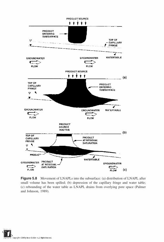
Figure 5.8 Movement of LNAPLs into the subsurface: (a) distribution of LNAPL aftersmall volume has been spilled; (b) depression of the capillary fringe and water table;(c) rebounding of the water table as LNAPL drains from overlying pore space (Palmerand Johnson, 1989).

5.3.2 Dense Nonaqueous-Phase Liquids

Compared to the LNAPLs, the DNAPLs are more complex in the way they mi-grate in the subsurface. Only during the last decade have they been studied indetail and their movement conceptualized. The mobility of DNAPLs is greaterthan that of LNAPLs because they are denser than water and most of them havelow viscosity. The relatively high density of the DNAPLs carries the productdeep into the aquifers, hundreds of feet below the ground surface in somecases.

Similar to LNAPLs, the DNAPLs enter into the soil–water–air system ofthe unsaturated zone under the influence of gravity. However, unlike LNAPLs,the DNAPLs are known to exhibit fingering behavior (Fig. 5.9a) when the unsatu-rated soil is relatively wet. This finguring phenomenon has been established tobe the result of a high-density, low-viscosity fluid (DNAPL) displacing a lower-density, higher-viscosity fluid (water) (Kueper and Frind, 1988). No finguringoccurs, however, if the soil is dry. When a sufficient quantity of DNAPL is re-leased, it advances to the water table, and unlike LNAPLs, it penetrates into theaquifer. The DNAPL is, however, still a nonwetting fluid compared to water,therefore it must overcome capillary forces in order to penetrate into the poresof the soil–water system. As discussed earlier, the DNAPL must possess an entryor threshold pressure sufficient to overcome the capillary forces. The higher den-sity of the DNAPLs contributes to this entry pressure. If the DNAPL pressureis higher than the entry pressure, the DNAPL proceeds into the soil–water systemuntil the source is exhausted. A finer-grained stratum in the unsaturated zonemay sometimes stop the DNAPL migration (Fig. 5.9b), because finer-grainedmaterials possess finer pores, which are associated with higher entry pressure. Ifthe DNAPL source is larger, it may penetrate the entire thickness of the aquiferand settle down on the impermeable stratum at the bottom of the aquifer (Fig.5.9c). In cases where the impermeable stratum is sloping, the DNAPL tends toflow down the dip of the stratum, which may be in a direction opposite to thatof the groundwater flow in the aquifer. This causes problems in characterizingthe source of the DNAPL, since the dissolved phase may be transported in adirection different from that of the free product.

The transport of DNAPLs is tremendously complicated by field-scale heter-ogeneities. The examples shown in Figure 5.10 demonstrate the challenges asso-ciated with characterizing DNAPL penetration in the subsurface. Figure 5.10ashows a scenario where a rock stratum exists between a surficial sand layer andthe water table. The rock stratum may be fractured with cracks of various lengths,widths, and apertures. These cracks convey the DNAPLs either into the dead-end zones or, through interconnectedness, directly to the water table. Character-ization of DNAPL penetration into a fractured rock is a challenge that the scien-tific community has only begun to face. Figure 5.10b shows the DNAPL transport

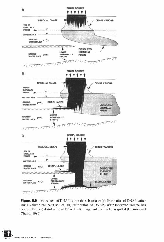
Figure 5.9 Movement of DNAPLs into the subsurface: (a) distribution of DNAPL aftersmall volume has been spilled; (b) distribution of DNAPL after moderate volume hasbeen spilled; (c) distribution of DNAPL after large volume has been spilled (Feenstra andCherry, 1987).

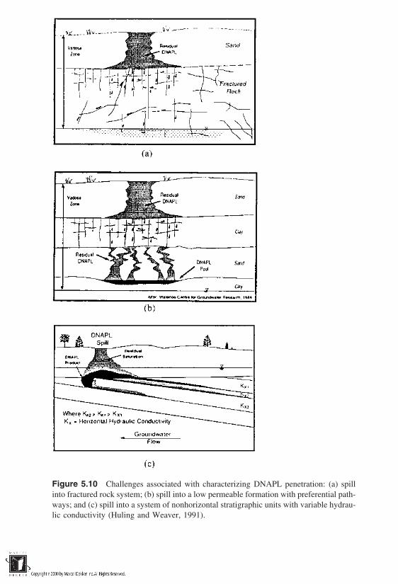
Figure 5.10 Challenges associated with characterizing DNAPL penetration: (a) spillinto fractured rock system; (b) spill into a low permeable formation with preferential path-ways; and (c) spill into a system of nonhorizontal stratigraphic units with variable hydrau-lic conductivity (Huling and Weaver, 1991).

through a layered system where the clay layer may contain a heterogeneous distri-bution of preferential pathways. Entry pressures based on the homogeneous pore-size distribution of the clay may be high, yet the DNAPL can migrate throughthe preferential pathways and convey the DNAPL into strata below the clay layer.Figure 5.10c shows the possibility of DNAPLs flowing in directions differentfrom that of the groundwater flow. Inclined strata of different hydraulic conduc-tivities may convey DNAPLs to considerable distances upstream of the locationof the spill.

5.4 PHASE DIAGRAM FOR SOIL–WATER–LNAPL–AIRSYSTEMS

Estimation of the volumetric contents of the three phases of air, water, and NAPLis an essential component in modeling the transport of NAPLs in the subsurface.The relationships between capillary pressure and volumetric water contents ofNAPL, water, and air will form the constitutive expressions in transport model-ing. Substantial advances have been made recently to develop these relationshipsfor LNAPLs. Lenhard and Parker (1987, 1990) and Parker and Lenhard (1987)extended moisture rentention expressions in the unsaturated flow to account forthe presence of the NAPL phase. The resulting expressions, which will be de-scribed below, were validated in laboratory investigations (Lenhard and Parker,1988) and were used to calibrate field-scale observations in monitoring wells(Ostendorf et al., 1993).

The phase composition in the vicinity of groundwater table is illustratedin Figure 5.11, where dw and dl represent the depths to the water table and to thetop of the free product, respectively. The thickness of the LNAPL pool, whichaccumulates as a pancake at the top of the water table, is therefore equal to (dw dl). If a monitoring well is drilled in a LNAPL-contaminated site, free LNAPLproduct will be observed up to a height of (dw dl) above the water table. Inthe range, dw d dl, only LNAPL and water exist in the pore space. Immedi-ately above this range, the free LNAPL exists in combination with water and air.Above a depth d dm, the free product is not found and only water and aircoexist. Apart from air, water, and free LNAPL, a fourth phase is also presentin the form of trapped LNAPL ganglia encompassed by free water. As explainedearlier, this phase is a result of the fluctuating water table.

At a given depth, the interfacial tensions between air, LNAPL, and watergovern the radii of pore throats into which the various phases can penetrate. Thisfollows directly from Eq. (5.4). Because of capillarity, small pores are alwaysfilled with the wetting fluid. The interfacial tension between air and LNAPLusually corresponds to a large radius of curvature. If this radius is r1, all poresgreater than size r1 are filled with air and those smaller than r1 are filled with

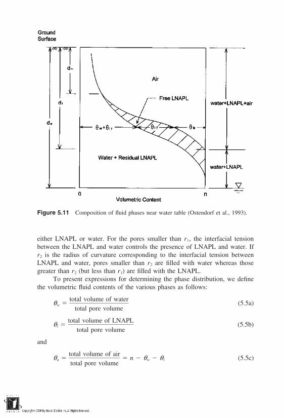
Figure 5.11 Composition of fluid phases near water table (Ostendorf et al., 1993).

either LNAPL or water. For the pores smaller than r1, the interfacial tensionbetween the LNAPL and water controls the presence of LNAPL and water. Ifr2 is the radius of curvature corresponding to the interfacial tension betweenLNAPL and water, pores smaller than r2 are filled with water whereas thosegreater than r2 (but less than r1) are filled with the LNAPL.

To present expressions for determining the phase distribution, we definethe volumetric fluid contents of the various phases as follows:

θw total volume of water

total pore volume(5.5a)

θ l total volume of LNAPL

total pore volume(5.5b)

and

θa total volume of airtotal pore volume

n θw θ l (5.5c)

where n porosity of the soil. Considering that both LNAPL and water existin free and residual forms,

θw θwr θwf (5.6a)

and

θ l θ lr θ lf (5.6b)

Effective saturation of water (Sw) and that of the total liquids (water and LNAPL),S, may be defined in terms of the above volumetric contents as

Sw (θw θ lr) θwr

n θwr

(5.7a)

S (θw θ lf θ lr) θwr

n θwr

(5.7b)

Note that the effective saturation of water includes the residual content ofLNAPL. The effective saturations of LNAPL in its free and residual form maybe defined similarly as

Slf θ lf

n θwr

S Sw (5.8a)

and

Slr θ lr

n θwr

(5.8b)

The effective saturations Sw and S, defined in Eq. (5.7), are governed by theinterfacial tensions between LNAPL and air, and between LNAPL and water.These are analogous to the effective saturation of water in soil–water–air sys-tems, where the moisture content above the water table is governed by the surfacetension of water. Therefore, the moisture retention functions, dealt with in Section3.6, can be adopted here for the purpose of relating S and Sw to the capillarypressures. Using van Genuchten’s (1980) function for water retention, Lenhardand Parker (1990) expressed S as

S 1 [β l(dl d )]α(1/α)1 (dl d dm) (5.9a)

and

S 1 (d dl) (5.9b)

where α empirical coefficient dependent on the pore size distribution of soils,and β l is a scaling factor, which is related to the interfacial tension betweenLNAPL and water and the mean pore radius, by

β l ρ lgrm

2σ la

(5.10)

where ρl density of the LNAPL, g acceleration due to gravity, rm meanpore radius, and σ la interfacial tension between LNAPL and air. Note that Eq.(5.10) is the capillary equation with contact angle assumed to be zero and thepores assumed to be cylindrical. Similarly, the effective saturation of water, Sw,is expressed as

Sw 1 [βw(dw d )]α(1/α)1 (dw d dm) (5.11a)

Sw 1 (d dw) (5.11b)

and

Sw 1 βlσ la

σwadl dw

ρw

ρldw d

α

(1/α)1

(dm d) (5.11c)

where σwa interfacial tension between water and air, i.e., the surface tension,ρw density of water, and βw is a scaling factor given by

βw βl[(ρw/ρ l) 1]σ la

σwl

(5.12)

where σwl interfacial tension between the water and the LNAPL phases. Thedepth dm to which the LNAPL free product rises above the water table can beobtained by equating Sw[Eq. (5.11a)] and S [Eq. (5.9a)], which will result in

dm β ldl βwdw

βl βw

(5.13)

Once S and Sw are determined through Eqs. (5.9) and (5.11), Slf can be determinedusing Eq. (5.8a). The only other quantity that needs to be determined is Slr, inorder to estimate the total volume of LNAPL in the soil with respect to depth.

As discussed earlier, the reason for residual entrapment of LNAPLs is thefluctuating water table, which causes changes in capillary pressures of the fluidsat a given point. Following Ostendorf et al. (1993) and Parker and Lenhard(1987), the hysteretic entrapment of LNAPLs in water is shown conceptually inFigure 5.12. Consider the changes in capillary pressure at point A, located at adepth d below the ground surface, as the water table fluctuates between the depthsof dw,min and dw,max (Fig. 5.12a). We choose the depth d such that d dm, sinceresidual entrapment of LNAPLs is possible only when free product is available.The corresponding retention curves are shown in Figure 5.12b. As the water tableis lowered from B to C, the water content at point A reduces along the path BC

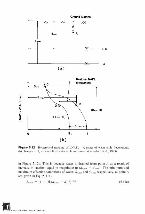
Figure 5.12 Hysteretical trapping of LNAPL: (a) range of water table fluctuations;(b) changes in Sw as a result of water table movement (Ostendorf et al., 1993).

in Figure 5.12b. This is because water is drained from point A as a result ofincrease in suction, equal in magnitude to (dw,max dw,min). The minimum andmaximum effective saturations of water, Sw,min and Sw,max respectively, at point Aare given in Eq. (5.11a),

Sw,min 1 [βw(dw,max d)]α(1/α)1 (5.14a)

and

Sw,max 1 [βw(dw,min d)]α(1/α)1 (5.14b)

When the water table moves upward from C to D, the moisture characteristicpath does not coincide with CB (Fig. 5.12b) because of hysteresis; instead, itfollows the path CD. Some of the free LNAPL is trapped during this stage, themagnitude of which is equal to BD in Figure 5.12b. If in fact the water tablerises past the point A under consideration, the amount of residual LNAPL entrap-ment at the point is equal to Slr,max. This is the maximum entrapment that canoccur at point A and is given by Parker and Lenhard (1987)

Slr,max 1 Sw,min

1 γ(1 Sw,min)(5.15)

where γ is a hysteretical trapping factor defined by the hysteresis in the contactangle and the radii of curvature at the interfaces. It is not possible to obtain valuesof γ directly. Published estimates of its magnitude were obtained by calibrationprocedures. Using residual LNAPL saturation data available at an aviation gaso-line spill site in Traverse City, Michigan, Ostendorf et al. (1993) obtained anestimate of γ 40. The soils at the site were characterized as medium-graineduniform sands with a mean particle diameter of 3.8 104 m.

In order to estimate residual saturations of LNAPLs at elevations higherthan the water table, such as BD in Figure 5.12b, Parker and Lenhard (1987)proposed the following empirical relationships:

Slr Slr,max 1 1 Sw,max

1 Sw,min dw,min d (5.16a)

Slr Slr,max dw,max d dw,min (5.16b)

Slr 0 0 d dm (5.16c)

and

Slr 0 d dmax (5.16d)

Equations (5.8a), (5.9), (5.11), and (5.16) completely describe the phase diagramand enable estimation of the volumetric contents of each of the phases in thevicinity of the water table.

5.5 MODELING TRANSPORT OF NAPLs IN SOILS

Modeling the transport of NAPLs in soils is complicated because of the multiplephases involved and the vast number of parameters associated with these phases.

As a result, prediction of NAPL migration in soils has remained as an academicand research endeavor only. We will present below essential principles involvedin NAPL transport, restricting the scope to a qualitative treatment of the problem.

5.5.1 Relative Permeability Concept

The transport of NAPLs is analogous to that of flow of water in unsaturated soilsin two respects: (1) the effective saturations of the phases keep on changing, and(2) the changes in the effective saturations in turn cause changes in the drivingforce for fluid flow. Darcy’s law is again invoked as the constitutive relationshipgoverning the flow of each of the three fluid phases, i.e., NAPL, water, and air.In order to use the Darcy’s law to express flow of air and NAPL, the hydraulicconductivity term is replaced by the intrinsic permeability (with the units of area),or

Vα kραg

µα∇φ (5.17)

where Vα velocity of the phase α, k intrinsic permeability of the medium,g acceleration due to gravity, ρα, µα density and dynamic viscosity of phaseα, respectively, and ∇φ potential gradient of the phase α.

As discussed in Chapter 3, the permeability of a fluid varies with the volu-metric content of that fluid. When NAPL, water, and air coexist in the pores, thepermeability of the medium with respect to any individual fluid is less than whenthe pore space is entirely occupied by that fluid. This reduction in permeabilityis dependent on the effective saturation of that fluid, and is described in termsof relative permeability, krα, which is defined as

krα kα (Sα)

ksα(5.18)

where kα(Sα) permeability of the soil with respect to phase α at effective satura-tion Sα, and ksα permeability of the soil at complete saturation with phase α.Thus, the relative permeability varies from 1.0 at complete saturation of the phaseto 0 near 0% saturation. In between 0 and 1.0, the fluids hinder the flow of eachother in the pore space.

Considering a two-phase system with only water and NAPL, the variationof the relative permeability with effective saturation is shown in Figure 5.13. Asthe effective saturation of water decreases from 100%, its relative permeabilityalso decreases. The relative permeability of the soil with respect to water becomeszero at a point where the water phase is no longer continuous and is at irreduciblesaturation. Similarly, as the effective saturation of the NAPL decreases from100%, its relative permeability also decreases, ultimately becoming zero at its

Figure 5.13 Relative permeabilities of water and NAPL as a function of the degree ofsaturation.

residual saturation. Because of the interference between the phases, the sum ofthe relative permeabilities (with respect to water and NAPL) do not equal 1.Thus, the overall permeability of the medium is reduced because of this interfer-ence. Three regions of flow can be delineated in Figure 5.13. In region I, NAPLdominates the pore space, and the relative permeability with respect to water isnearly zero. In region II, both NAPL and water exist in a continuous form andflow together. In this region, the interferences from each other are maximum,and the permeability of the medium as a whole is greatly reduced. In region III,water dominates the pore space, and the relative permeability with respect toNAPL is nearly zero because the NAPL is present in discontinuous form.

The above concept can be extended to a three-phase system when air ispresent in addition to NAPL and water. This is usually presented in a ternarydiagram as shown in Figure 5.14. The process is considerably more complicatedthan a two-phase system, although the same principles govern. It can be notedin Figure 5.14 that there are large areas where at least one of the fluids becomesimmobile. Also, all three fluids can flow simultaneously only in an extremely

Figure 5.14 Relative permeabilities for three-phase flow (Van Dam, 1967).

limited saturation region. Note that air also has a residual saturation, which hin-ders the permeability of the other two phases.

In most cases of NAPLs, data describing the relative permeability variationwith respect to effective saturations are not available. Both theoretical and empiri-cal equations were developed in the literature describing the variations (Stone,1973; Lenhard and Parker, 1987). Mathematical details of these equations arebeyond the scope of this fundamental treatment.

5.5.2 Equations Governing Multiphase Transport

As in the transport of water (Chapter 3) and dissolved solutes (Chapter 4), thetransport of NAPLs involves combination of the mass conservation principle andconstitutive (or cause-and-effect) relationships. However, the NAPL transportmodeling is far more complicated because of the multiple number of phases in-volved and possible interphase transfer of fluids. The transport of each of thephases is coupled with capillary pressures and effective saturations of the otherphases. In general, governing equations for each of the three phases are developedindividually and then they are coupled together using capillary pressure and effec-tive saturations. Although simple in principle, NAPL transport modeling requires

a vast number of parameters, not all of which can be obtained through routineexperiments.

Abriola and Pinder (1985a, 1985b) and Abriola (1988) presented a compre-hensive approach to modeling multiphase transport. Following this approach, webegin with a comprehensive statement of the transport problem by expressingthe mass balance of a chemical species i in the α phase as

∂∂ t

(ραεαωαi) ∇ ⋅ (ραεαVαωα

i) ∇ ⋅ J αi Aα

i Bαi (5.19)

where

ρα mass density of the α phaseεα fraction of pore volume occupied by the α phase

ωαi mass fraction of species i in the α phase

Vα velocity of the α phaseJα

i nonadvective flux of the species i in the α phaseAα

i exchange of mass of species i due to interphase diffusion and/orphase change

Bαi external supply of species i to the α phase

∇ differential operator

The first term represents the time rate of change in mass of species i in phaseα. The second and third terms reflect mass transport of species i due to advectionand nonadvective effects (diffusion and dispersion), respectively. The terms onthe right-hand side of the equation represent sink/source terms due to phasechanges, and chemical and biological reactions leading to destruction or creationof the species.

In order to express total mass balance of the species i in the system, asummation of mass balances in the individual phases should be carried out, or

α ∂

∂ t(ραεαω α

i) ∇ ⋅ (ραεαVαωαi) ∇ ⋅ J α

i α

Bαi (5.20)

Note that the above equation does not contain the term Aαi representing exchange

of species mass among the phases, since mass lost by one phase is gained by theother phases, i.e.,

α

Aαi 0 (5.21)

Also, the summation should be carried out including soil solids as a separatephase to account for the compressibility of the porous medium and species masspresent in the adsorbed form. Equations such as (5.20) are known as species-

balance or compositional equations. One such equation has to be solved for eachof the species present in the system.

Equations (5.19) and (5.20) may be simplified by assuming ∇ ⋅ J αi 0,

in the case of those species which maintain a sharp wetting front and whichmay not be transported by nonadvective means such as diffusion and dispersion.Assuming that Darcy’s law is a valid constitutive relation, Vα may be expandedin Eq. (5.19) and the resulting set of equations for the water, NAPL, and airphases may be expressed for a single-species chemical as

∂∂ t

(ρwnSwωw) ∇ ⋅ kρwkrw

µw

(∇ ⋅ Pw ρwg∇ ⋅ Dw) Aw Bw (5.22a)

∂∂ t

(ρnnSnωn) ∇ ⋅ kρnkrn

µn

(∇ ⋅ Pn ρng∇ ⋅ Dn) An Bn (5.22b)

and

∂∂ t

(ρanSaωa) ∇ ⋅ kρakra

µa

(∇ ⋅ Pa ρag∇ ⋅ Da) Aa Ba (5.22c)

where subscripts w, n, and a, stand for water, NAPL, and air phases, respectively,Da elevation head of the phase α, Pα pressure head of the phase α, and allother terms are as defined earlier. Solution of Eqs. (5.22) involves 18 variables:ρw, ρn, ρa, Sw, Sn, Sa, krw, krn, kra, µw, µn, µa, ωw, ωn, ωa, Pw, Pn, and Pa. Therefore,in addition to the three equations above, 15 more equations are needed for com-plete solution of the problem. These may be obtained as follows.

1. Densities (ρw, ρn, ρa) and viscosities (µw, µn, µa) may be expressed asknown functions of pressures (Pw, Pn, Pa), yielding six equations.

2. Effective saturations (Sw, Sn, Sa) may be expressed as functions of pres-sures (Pw, Pn, Pa), yielding three equations.

3. Relative permeabilities (krw, krn, kra) may be expressed as functions ofeffective saturations, yielding three equations.

4. Mass fractions of species in all the phases may be assumed to be atlocal equilibrium, which implies that the time scales are such that ad-joining phases reach a thermodynamic equilibrium. This will yield twoexpressions of the form

ωα κ αβωβ (5.23)

where καβ is known as the partition coefficient of the species betweenα and β phases. These coefficients are functions of phases composi-tions and pressures and may be determined using Henry’s law andRaoult’s law constants. Therefore, two equations of the type (5.23)together with ∑αωα 1 will give three equations in total.

Note that the soil phase is ignored in Eq. (5.22). The soil is assumed to beincompressible and porosity is assumed to be constant. Further simplification ofthe above system of equations is possible when the gas phase remains at atmo-spheric pressure, in which case Eq. (5.22c) can be reduced to a simpler form.

5.6 MOBILIZATION OF RESIDUAL NAPLs

In modeling the transport of NAPLs in Section 5.5, we ignored the discontinuous/residual phase of NAPLs. This is justifiable because the residual content ofNAPLs is relatively immobile. In remediation operations, however, the residualcontent of NAPLs often amounts to significant quantities, and its mobilizationand recovery are important. Unlike free product removal, residually trapped gan-glia are difficult to mobilize. Research on mobilization of NAPL ganglia was firstinitiated in the petroleum engineering discipline in the context of enhancement ofrecoveries from subsurface oil reservoirs. The principles developed in that disci-pline were later adopted in environmental engineering in the context of subsur-face remediation. Due to recent emphasis on in-situ remediation, several researchefforts have focused lately on the mechanics of entrapment and the mobilizationof ganglia.

Entrapment of ganglia is a pore-scale phenomenon, therefore an under-standing of their transport must begin at pore scale. Although several modes ofganglion entrapment have been conceptualized in the literature, two modes arecommonly accepted for a soil–water–NAPL system: snap-off and bypassing(Chatzis et al., 1983). Snap-off occurs when the NAPL is displaced from a porebody into a pore throat by water (Fig. 5.15). Water moves along the sides of thepores, where it displaces the NAPL, and reaches the end of the pore body beforeNAPL can exit. As water begins to enter the pore throat, NAPL ‘‘snaps-off’’and remains in the pore as a trapped ganglion. As shown in Figure 5.15a, thismode of entrapment is likely in cases where the aspect ratio of the pores (theratio of the size of the pore body to that of the pore throat) is high. When theaspect ratio is small, complete displacement of the NAPL is possible, as shownin Figure 5.15b. The likelihood of snap-off also depends on the wettability ofthe two liquids. Snap-off occurs in systems where the media are water-wet. Ifthey are intermediate-wet (θ 90°), snap-off may not occur.

Bypassing, on the other hand, occurs when the NAPL is displaced by waterin a complex pore structure and is described using a pore doublet model (Chatziset al., 1983). As shown in Figure 5.16a, the pore doublet model is visualizedusing two arms of a pore. Bypassing does not occur when the two arms havesimilar geometry. However, as shown in Figure 5.16b, when the downstreamnode of the upper arm is smaller than that of the lower arm, the advancing waterwill bypass the NAPL in the lower arm. The greater capillary force associated

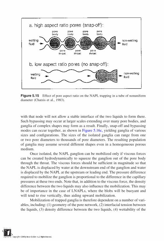
Figure 5.15 Effect of pore aspect ratio on the NAPL trapping in a tube of nonuniformdiameter (Chatzis et al., 1983).

with that node will not allow a stable interface of the two liquids to form there.Such bypassing may occur at larger scales extending over many pore bodies, andganglia of complex shapes may form as a result. Finally, snap-off and bypassingmodes can occur together, as shown in Figure 5.16c, yielding ganglia of varioussizes and configurations. The sizes of the isolated ganglia can range from oneor two pore diameters to thousands of pore diameters. The resulting populationof ganglia may assume several different shapes even in a homogeneous porousmedium.

Once isolated, the NAPL ganglion can be mobilized only if viscous forcescan be created hydrodynamically to squeeze the ganglion out of the pore bodythrough the throat. The viscous forces should be sufficient in magnitude so thatthe NAPL is displaced by water at the downstream end of the ganglion and wateris displaced by the NAPL at the upstream or leading end. The pressure differencerequired to mobilize the ganglion is proportional to the difference in the capillarypressures at these two ends. Note that, in addition to the viscous force, the densitydifference between the two liquids may also influence the mobilization. This maybe of importance in the case of LNAPLs, where the blobs will be buoyant andwill tend to rise vertically, thus aiding upward mobilization.

Mobilization of trapped ganglia is therefore dependent on a number of vari-ables, including: (1) geometry of the pore network, (2) interfacial tension betweenthe liquids, (3) density difference between the two liquids, (4) wettability of the

Figure 5.16 Conceptualization of NAPL trapping mechanisms using the pore doubletmodel (Chatzis et al., 1983).

medium by the two liquids, and (5) applied water-phase pressure gradient andits alignment with gravity. For soil–NAPL–water systems, these parameters areconveniently incorporated into two dimensionless numbers: capillary number,Nc, which is the ratio of viscous forces to capillary forces; and bond number,Nb, which is the ratio of gravity forces to capillary forces. Three different versionsfor capillary number Nc are used in the literature:

N1c

Vwµw

σnw

(Melrose and Brandner, 1974; Morrow andSongkran, 1981) (5.24a)

N 2c

k∇P

σnw

(Ojeda et al., 1953; Larson et al., 1981) (5.24b)

N 3c

KJµw

σnw

(Wilson and Conrad, 1984; Wilson et al., 1990) (5.24c)

where the superscript is used to denote the version of the capillary number, K water-saturated hydraulic conductivity of soil (L/T); ∇P water phase pressure

gradient expressed as (F/L3); and J hydraulic gradient in the water phase (in-cluding gravity), and all other terms are as defined earlier. All of these versionsare equivalent in the sense that the numerator indicates a measure of the viscousforce and the denominator indicates the capillary force. The bond number, Nb,also has been used in two different forms (Morrow and Songkran, 1981):

N1b

∆ρgR2

σnw

(5.25a)

N 2b

∆ρgk

σnw

(5.25b)

where ∆ρ density difference between water and NAPL, g acceleration dueto gravity, and R representative grain radius in the soil. Clearly, the intrinsicpermeability of soil is related to the grain size, therefore the two equations areequivalent in nature. In random packings of uniform spheres, the relationshipbetween R and k may be expressed as (Morrow and Songkran, 1981)

k 0.00317R2 (5.26)

which, when substituted in Eq. (5.25), yields

N 2b 0.00317N 1

b (5.27)

Most of the research on mobilization of NAPL ganglia was conducted in anattempt to correlate the mobilization with the capillary number. Although densitydifferences influence mobilization, the effect of these forces were often consid-ered to be negligible in comparison with viscous forces. Typical residual satura-tion versus capillary number curves for glass beads and sandstones containingNAPL ganglia are shown in Figure 5.17. The y axis represents the reduced resid-ual saturation as a ratio of residual saturation at a given capillary number to theinitial residual saturation. As seen in Figure 5.17, a minimum capillary number(indicated as N*c ) is required to initiate mobilization of the ganglia from theirinitial state. Its magnitude is 2 105 for the sandstone curve and about 1 103 for the bead-pack. N**c represents the capillary number required to mobilizeall of the entrapped ganglia; N**c 1.3 103 for sandstones and 9 103 forbead pack. In order to achieve these capillary numbers, the water phase pressuregradient must be increased for a given soil–water–NAPL system.

The data from Figure 5.17 may be replotted as in Figure 5.18 for a betterunderstanding of the range of hydraulic gradients required to mobilize the NAPLganglia in a soil–NAPL–water system. Obviously, for NAPLs with smaller in-terfacial tensions, lower hydraulic gradients are needed to achieve N**c . As anexample, consider the gradients required to initiate mobilization of NAPL gangliawith an interfacial tension of 10 dynes/cm. If the porous medium represents afine gravel with k 105 cm2, a gradient J 102 is required. To remove all

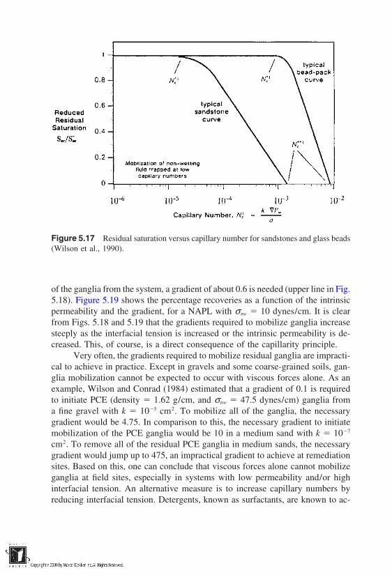
Figure 5.17 Residual saturation versus capillary number for sandstones and glass beads(Wilson et al., 1990).

of the ganglia from the system, a gradient of about 0.6 is needed (upper line in Fig.5.18). Figure 5.19 shows the percentage recoveries as a function of the intrinsicpermeability and the gradient, for a NAPL with σnw 10 dynes/cm. It is clearfrom Figs. 5.18 and 5.19 that the gradients required to mobilize ganglia increasesteeply as the interfacial tension is increased or the intrinsic permeability is de-creased. This, of course, is a direct consequence of the capillarity principle.

Very often, the gradients required to mobilize residual ganglia are impracti-cal to achieve in practice. Except in gravels and some coarse-grained soils, gan-glia mobilization cannot be expected to occur with viscous forces alone. As anexample, Wilson and Conrad (1984) estimated that a gradient of 0.1 is requiredto initiate PCE (density 1.62 g/cm, and σnw 47.5 dynes/cm) ganglia froma fine gravel with k 105 cm2. To mobilize all of the ganglia, the necessarygradient would be 4.75. In comparison to this, the necessary gradient to initiatemobilization of the PCE ganglia would be 10 in a medium sand with k 107

cm2. To remove all of the residual PCE ganglia in medium sands, the necessarygradient would jump up to 475, an impractical gradient to achieve at remediationsites. Based on this, one can conclude that viscous forces alone cannot mobilizeganglia at field sites, especially in systems with low permeability and/or highinterfacial tension. An alternative measure is to increase capillary numbers byreducing interfacial tension. Detergents, known as surfactants, are known to ac-

Figure 5.18 Hydraulic gradient required to initiate blob mobilization in porous mediaof various permeabilities, for organic liquids of various interfacial tensions (Wilson et al.,1990).

complish this to some extent. Development of innovative methods to clean upsites contaminated with residual NAPL ganglia is an area of intense research atpresent.

5.7 MASS TRANSFER PROCESSES

The sink-source terms in the governing equation for NAPLs transport [Eq. (5.19)]arise from a number of mass transfer processes occurring simultaneously amongall the phases involved. As shown in Figure 5.20, the main processes pertinent toNAPLs are dissolution, sorption, and volatilization. Of these, dissolution deservesadditional discussion in the context of NAPLs. It controls the movement ofNAPLs to a great extent. For example, chlorinated solvents, which are onlyslightly soluble in water, penetrate deep into aquifers and remain as an immiscible

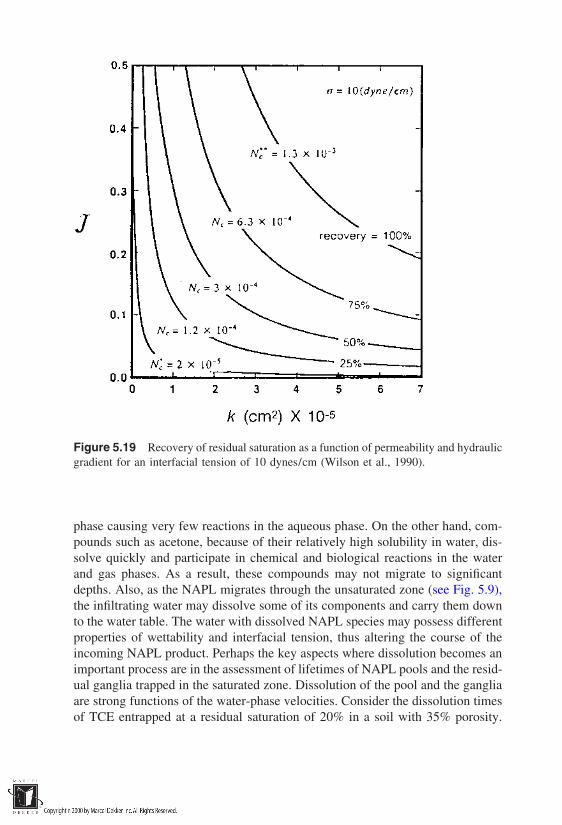
Figure 5.19 Recovery of residual saturation as a function of permeability and hydraulicgradient for an interfacial tension of 10 dynes/cm (Wilson et al., 1990).

phase causing very few reactions in the aqueous phase. On the other hand, com-pounds such as acetone, because of their relatively high solubility in water, dis-solve quickly and participate in chemical and biological reactions in the waterand gas phases. As a result, these compounds may not migrate to significantdepths. Also, as the NAPL migrates through the unsaturated zone (see Fig. 5.9),the infiltrating water may dissolve some of its components and carry them downto the water table. The water with dissolved NAPL species may possess differentproperties of wettability and interfacial tension, thus altering the course of theincoming NAPL product. Perhaps the key aspects where dissolution becomes animportant process are in the assessment of lifetimes of NAPL pools and the resid-ual ganglia trapped in the saturated zone. Dissolution of the pool and the gangliaare strong functions of the water-phase velocities. Consider the dissolution timesof TCE entrapped at a residual saturation of 20% in a soil with 35% porosity.

Figure 5.20 Mass transfer processes involved in partitioning of NAPLs into solid, wa-ter, and gas phases.

Palmer and Johnson (1989) estimate that it would take 15.4 years for the gangliato be completely dissolved in a cubic meter of the soil when subjected to a contin-uous flow rate of 1.7 cm/day. NAPLs with lower solubility than TCE wouldrequire even longer periods, often up to several decades.

The aqueous solubilities of NAPL species govern to a great extent the timerate of pool and ganglia dissolution. As shown in Tables 5.1 and 5.2, the solubilit-ies of NAPLs vary greatly. For NAPLs comprised of a mixture of several species,an effective solubility is often used. It is defined as the aqueous solubility ofan organic constituent which is in chemical equilibrium with a NAPL mixtureconsisting of several such organic constituents. It can be estimated as a productof the mole fraction of the organic constituent in the NAPL mixture and its purephase solubility.

In addition to the solubility of the NAPL in water, dissolution from NAPLstrapped in the form of ganglia is governed by the porosity of the medium, sizeand shape of the individual ganglia, and aqueous phase velocity. Several mathe-matical derivations exist in the literature correlating the flux from a dissolving

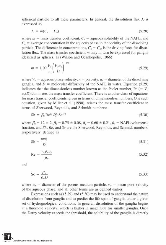
spherical particle to all these parameters. In general, the dissolution flux Jd isexpressed as

Jd m(Cs Ca) (5.28)

where m mass transfer coefficient, Cs aqueous solubility of the NAPL, andCa average concentration in the aqueous phase in the vicinity of the dissolvingparticle. The difference in concentrations, Cs Ca, is the driving force for disso-lution flux. The mass transfer coefficient m may in turn be expressed for gangliaidealized as spheres, as (Wilson and Geankopolis, 1966)

m 1.09Vw

n Vwan

D 2/3

(5.29)

where Vw aqueous phase velocity, n porosity, an diameter of the dissolvingganglia, and D molecular diffusivity of the NAPL in water. Equation (5.29)indicates that the dimensionless number known as the Peclet number, Pe ( Vw

an/D) dominates the mass transfer coefficient. There is another class of equationsfor mass transfer coefficients, given in terms of dimensionless numbers. One suchequation, given by Miller et al. (1990), relates the mass transfer coefficient interms of Sherwood, Reynolds, and Schmidt numbers:

Sh β0 Reβ1 θβ2n Sc1/2 (5.30)

where β0 12 2, β1 0.75 0.08, β2 0.60 0.21, θn NAPL volumetricfraction, and Sh, Re, and Sc are the Sherwood, Reynolds, and Schmidt numbers,respectively, defined as

Sh ma2

p

D(5.31)

Re vwρwap

µw

(5.32)

and

Sc µw

ρwD(5.33)

where ap diameter of the porous medium particle, vw mean pore velocityof the aqueous phase, and all other terms are as defined earlier.

Expressions such as (5.29) and (5.30) may be used to understand the natureof dissolution from ganglia and to predict the life span of ganglia under a givenset of hydrogeological conditions. In general, dissolution of the ganglia beginsat a threshold velocity, which is higher in magnitude for smaller ganglia. Oncethe Darcy velocity exceeds the threshold, the solubility of the ganglia is directly

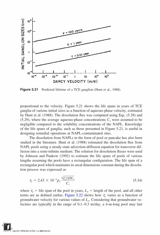
Figure 5.21 Predicted lifetime of a TCE ganglion (Hunt et al., 1988).

proportional to the velocity. Figure 5.21 shows the life spans in years of TCEganglia of various initial sizes as a function of aqueous-phase velocity, estimatedby Hunt et al. (1988). The dissolution flux was computed using Eqs. (5.28) and(5.29), where the average aqueous-phase concentrations Ca were assumed to benegligible compared to the solubility concentrations of the NAPL. Knowledgeof the life spans of ganglia, such as those presented in Figure 5.21, is useful indesigning remedial operations at NAPL-contaminated sites.

The dissolution from NAPLs in the form of pool or pancake has also beenstudied in the literature. Hunt et al. (1988) estimated the dissolution flux fromNAPL pools using a steady-state advection-diffusion equation for transverse dif-fusion into a semi-infinite medium. The solution for dissolution fluxes were usedby Johnson and Pankow (1992) to estimate the life spans of pools of variouslengths assuming the pools have a rectangular configuration. The life span of arectangular pool which maintains its areal dimensions constant during the dissolu-tion process was expressed as

τp 2.43 105ρn√L3

p/DVw

Cs

(5.34)

where τp life span of the pool in years, Lp length of the pool, and all otherterms are as defined earlier. Figure 5.22 shows how τp varies as a function ofgroundwater velocity for various values of Lp. Considering that groundwater ve-locities are typically in the range of 0.1–0.3 m/day, a 4-m-long pool may last

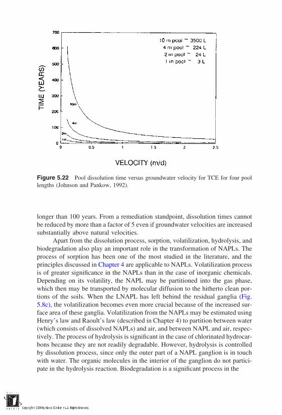
Figure 5.22 Pool dissolution time versus groundwater velocity for TCE for four poollengths (Johnson and Pankow, 1992).

longer than 100 years. From a remediation standpoint, dissolution times cannotbe reduced by more than a factor of 5 even if groundwater velocities are increasedsubstantially above natural velocities.

Apart from the dissolution process, sorption, volatilization, hydrolysis, andbiodegradation also play an important role in the transformation of NAPLs. Theprocess of sorption has been one of the most studied in the literature, and theprinciples discussed in Chapter 4 are applicable to NAPLs. Volatilization processis of greater significance in the NAPLs than in the case of inorganic chemicals.Depending on its volatility, the NAPL may be partitioned into the gas phase,which then may be transported by molecular diffusion to the hitherto clean por-tions of the soils. When the LNAPL has left behind the residual ganglia (Fig.5.8c), the volatilization becomes even more crucial because of the increased sur-face area of these ganglia. Volatilization from the NAPLs may be estimated usingHenry’s law and Raoult’s law (described in Chapter 4) to partition between water(which consists of dissolved NAPLs) and air, and between NAPL and air, respec-tively. The process of hydrolysis is significant in the case of chlorinated hydrocar-bons because they are not readily degradable. However, hydrolysis is controlledby dissolution process, since only the outer part of a NAPL ganglion is in touchwith water. The organic molecules in the interior of the ganglion do not partici-pate in the hydrolysis reaction. Biodegradation is a significant process in the

of LNAPLs such as benzene, toluene, and xylenes, which are known to be de-graded by indigenous aerobic microorganisms. In general, in-situ biodegradationof LNAPLs is limited by the supply of dissolved oxygen. DNAPLs, on the otherhand, are known to degrade only under anaerobic conditions or are resistant todegradation (Feenstra and Cherry, 1988).

REFERENCES

Abriola, L. M. (1988). Multiphase flow and transport models for organic chemicals: Areview and assessment. Electric Power Research Institute, EA-5976, Palo Alto, CA.

Abriola, L. M., and Pinder, G. F. (1985a). A multiphase approach to the modeling ofporous media contamination by organic compounds, 1. Equation development. Wa-ter Resources Res., 21(1):11–18.

Abriola, L. M., and Pinder, G. F. (1985b). A multiphase approach to the modeling ofporous media contamination by organic compounds, 2. Numerical simulation. Wa-ter Resources Res., 21(1):19–26.

Anderson, W. G. (1986). Wettability literature survey, Part 1. Rock/oil/brine interactions,and the effects of core handling on wettability. J. Petrol. Technol., Oct.: 1125–1149.

Chatzis, I., Morrow, N. R., and Lim, H. T. (1983). Magnitude and detailed structure ofresidual oil saturation. SPE J. 23(2):311–325.

Feenstra, S., and Cherry, J. A. (1987). Dense organic solvents in ground water: An intro-duction. In Dense Chlorinated Solvents in Ground Water, Institute for Ground Wa-ter Research, University of Waterloo, Progress Report 0863985, Waterloo, Ont.

Feenstra, S., and Cherry, J. A. (1988). Subsurface contamination by dense non-aqueousphase liquids (DNAPL) chemicals. Int. Groundwater Symp., Int. Assoc. Hy-drogeol., Halifax, N.S., May 1–4, 1988.

Huling, S. G., and J. W. Weaver. (1991). Dense nonaqueous phase liquids. Ground WaterIssue, EPA/540/4-91-002, Robert S. Kerr Environmental Research Laboratory,Ada, OK.

Hunt, J. R., Sitar, N., and Udell, K. S. (1988). Nonaqueous phase liquid transport andcleanup. 1. Analysis of mechanisms. Water Resources Res., 24(8):1247–1258.

Johnson, R. L., and Pankow, J. F. (1992). Dissolution of dense chlorinated solvents intogroundwater. 2. Source functions for pools of solvent. Environ. Sci. Technol., 26(5):896–901.

Kueper, B. H., and Find, E. O. (1988). An overview of immiscible fingering in porousmedia. J. Contam. Hydrol., 2:95–110.

Larson, R. G., Davis, H. T., and Scriven, L. E. (1981). Displacement of residual nonwet-ting fluid from porous media. Chem. Eng. Sci., 36:75–85.

Lenhard, R. J., and Parker, J. C. (1987). Measurement and prediction of saturation-pressurerelationships in three phase porous media systems. J. Contam. Hydrol., 1:407–424.

Lenhard, R. J., and Parker, J. C. (1988). Experimental validation of the theory of extendingtwo phase saturation-pressure relations to three fluid phase systems for monotonicdrainage paths. Water Resources Res., 24:373–380.

Lenhard, R. J., and Parker, J. C. (1990). Estimation of free hydrocarbon volume fromfluid levels in monitoring wells. Ground Water, 28:57–67.

Luckner, L., and Schestakow, W. M. (1991). Migration Processes in the Soil and Ground-water Zone. Lewis Publishers, Chelsea, MI.

Melrose, J. C., and Brandner, C. F. (1974). Role of capillary forces in determining micro-scopic displacement efficiency for oil recovery by waterflooding. J. Can. Petrol.Technol., 13(42):54–62.

Mercer, J. W., and Cohen, R. M. (1990). A review of immiscible fluids in the subsurface:Properties, models, characterization and remediation. J. Contam. Hydrol., 6:107–163.

Miller, C. T., Poirier-McNeill, M. M., and Mayer, A. S. (1990). Dissolution of trappednonaqueous phase liquids: Mass transfer characteristics. Water Resources Res.,26(11):2783–2796.

Morrow, N. R., and Songkran, B. (1981). Effect of viscous and buoyancy forces on non-wetting phase trapping in porous media. In D. O. Shah (ed.), Surface Phenomenain Enhanced Oil Recovery, pp. 387–411. Plenum, New York.

Ojeda, E., Preston, F., and Calhoun, J. C. (1953). Correlations of oil residuals followingsurfactant floods. Producers Monthly, 18(2):20.

Ostendorf, D. W., Richards, R. J., and Beck, F. P. (1993). LNAPL retention in sandy soil.Ground Water, 31(2):285–292.

Palmer, C. D., and Johnson, R. L. (1989). Physical processes controlling the transport ofnon-aqueous phase liquids in the subsurface. In Transport and Fate of Contaminantsin the Subsurface, EPA/625/4-89/019, Chap. 3. U.S. Environmental ProtectionAgency, September.

Parker, J. C., and Lenhard, R. J. (1987). A model for hysteretic constitutive relationsgoverning multiphase flow, I. Saturation pressure relations. Water Resources Res.,23:2187–2196.

Stone, H. L. (1973). Estimation of three-phase relative permeability and residual oil data.J. Can. Petrol. Technol., 12(4):53–61.

Van Dam, J. (1967). The migration of hydrocarbons in a water bearing stratum. In P.Hepple (ed.), The Joint Problems of the Oil and Water Industries, pp. 55–96. Inst.Petrol., London.

Van Genuchten, M. Th. (1980). A closed form equation for predicting the hydraulic con-ductivity of unsaturated soils. Soil Sci. Soc. Am. J., 44:892–898.

Wilson, E. J., and Geankopolis, C. J. (1966). Liquid mass transfer at very low Reynoldsnumbers in packed beds. Ind. Eng. Chem. Fundam., 5(1):9–14.

Wilson, J. L., and Conrad, S. H. (1984). Is physical displacement of residual hydrocarbonsa realistic possibility in aquifer restoration? In Proc., NWWA/API Conf. on Petro-leum Hydrocarbons and Organic Chemicals in Ground Water—Prevention, Detec-tion, and Restoration, pp. 274–298. National Water Well Association, Worthing-ton, OH.

Wilson, J. L., Conrad, S. H., Mason, W. R., Peplinski, W., and Hagan, E., (1990). Labora-tory investigation of residual liquid organics from spills, leaks, and the disposal ofhazardous wastes in groundwater, EPA/600/6-90/004. U.S. Environmental Protec-tion Agency, Robert S. Kerr Environmental Research Laboratory, Ada, OK.

6Site Characterization andContaminant Release Mechanisms

6.1 SITE CONTAMINATION SCENARIOS

Contaminated sites for which remediation schemes are usually designed and im-plemented vary with respect to configuration, contaminant releasing unit, sitehydrology, contaminant source relative to ground elevation, hydrogeological andgeotechnical characteristics of the host media, chemical characteristics, and con-centrations of contaminants. These factors are determinants of the hazards posedto human health and environment by any contaminated site. The most commonsite-specific sources of contaminants are

Solid waste management unitsLand treatment unitsSurface impoundmentsWaste pilesIncinerators and other industrial installationsTanks and other containers

A few of the site contamination scenarios that are associated with thesources listed above are illustrated in Figures. 6.1 and 6.2.

In Figure 6.1A, a landfill serves as the source of contaminants which haveleaked through flaws in its liner into the surrounding media. In Figure 6.1B, thesource is buried waste. No containment system was used. Consequently, wasteconstituents have migrated with little or no hindrance into the surrounding soil.The configuration shown in Figure 6.1B is representative of sources at relativelyold waste sites initiated before the past 30–40 years, during which waste ‘‘dump-ing’’ in unlined systems was common. Figure 6.1C shows a waste pile that liesdirectly on an unprotected ground surface. Particles of waste have migrated intothe ground. In general, the smaller the particle sizes of the waste relative to those

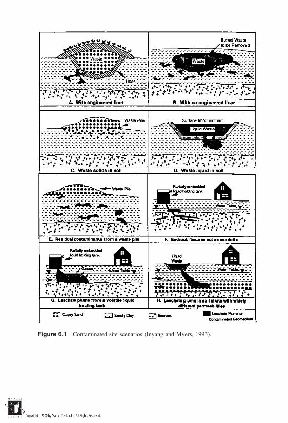
Figure 6.1 Contaminated site scenarios (Inyang and Myers, 1993).

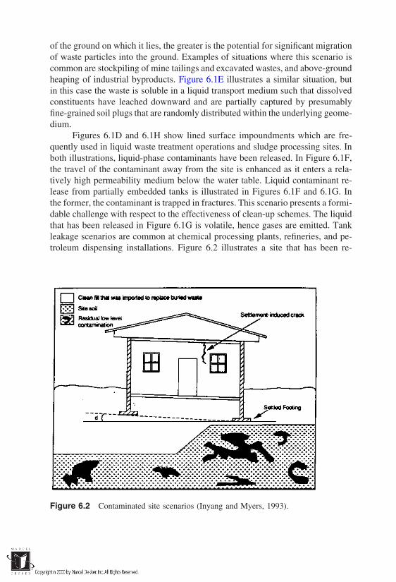
of the ground on which it lies, the greater is the potential for significant migrationof waste particles into the ground. Examples of situations where this scenario iscommon are stockpiling of mine tailings and excavated wastes, and above-groundheaping of industrial byproducts. Figure 6.1E illustrates a similar situation, butin this case the waste is soluble in a liquid transport medium such that dissolvedconstituents have leached downward and are partially captured by presumablyfine-grained soil plugs that are randomly distributed within the underlying geome-dium.

Figures 6.1D and 6.1H show lined surface impoundments which are fre-quently used in liquid waste treatment operations and sludge processing sites. Inboth illustrations, liquid-phase contaminants have been released. In Figure 6.1F,the travel of the contaminant away from the site is enhanced as it enters a rela-tively high permeability medium below the water table. Liquid contaminant re-lease from partially embedded tanks is illustrated in Figures 6.1F and 6.1G. Inthe former, the contaminant is trapped in fractures. This scenario presents a formi-dable challenge with respect to the effectiveness of clean-up schemes. The liquidthat has been released in Figure 6.1G is volatile, hence gases are emitted. Tankleakage scenarios are common at chemical processing plants, refineries, and pe-troleum dispensing installations. Figure 6.2 illustrates a site that has been re-

Figure 6.2 Contaminated site scenarios (Inyang and Myers, 1993).

claimed for building construction purposes. Residual contaminants are unevenlydistributed in the subsurface. Land recycling ‘‘brownfields redevelopment’’ is-sues and associated technologies have been described by Yland and van Wachem(1988), Anderson and Hatayama (1988), and Blacklock (1987).

6.2 CHARACTERIZATION OF CONTAMINATED SITES

The objectives of site characterization are multifaceted. They may include oneor more of the following:

Assessment of environmental/ecological settingsDetermination of the concentrations and spatial distributions of contami-

nantsAssessment of environmental and human health risks (including exposure)Determination of the treatability of sites and the most appropriate remedia-

tion techniques

Several basic questions usually need to be answered using data obtainedduring site characterization. Usually, the existence of data alone does not auto-matically imply that the objectives will be met. Analytical techniques need to beapplied to acquired data to seek answers to the following categories of questions:

What are the contaminants?In what physical forms are they?What is the source of the contaminants?Where are the contaminants and their boundaries?Are they stationary or are they still moving?What migration pathways are likely to be significant?What and where are the potential receptors of the contaminants relative to

the location of the release area?

It is advisable to develop a systematic approach to conducting site investi-gations to meet the intended objectives. For the site remediation objective whichis frequently the focus of activities, several approaches which spell out the se-quence of tasks as exemplified by Figure 6.3 (U.S. EPA, 1991) have been devel-oped. The reader should note that the flowchart presented in Figure 6.3 focusesprimarily on the site characterization tasks and relevant analyses needed to selecta remediation technology for a contaminated site. The flowchart would be differ-ent if the objective were to determine locations of highest hazard at a site.

Some specific numerical ranges of parameters categorized in Table 6.1 havedirect and measurable effects on the potential transport of contaminants from asource area. Rosenberg et al. (1990) have indexed the specific ranges for somesite and waste characteristics into low, medium, high, and other relevant designa-

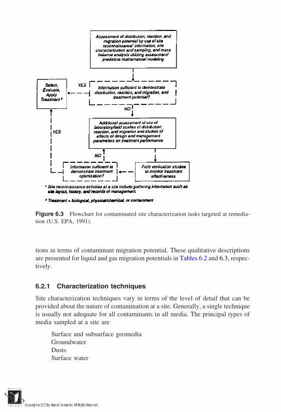
Figure 6.3 Flowchart for contaminated site characterization tasks targeted at remedia-tion (U.S. EPA, 1991).

tions in terms of contaminant migration potential. These qualitative descriptionsare presented for liquid and gas migration potentials in Tables 6.2 and 6.3, respec-tively.

6.2.1 Characterization techniques

Site characterization techniques vary in terms of the level of detail that can beprovided about the nature of contamination at a site. Generally, a single techniqueis usually not adequate for all contaminants in all media. The principal types ofmedia sampled at a site are

Surface and subsurface geomediaGroundwaterDustsSurface water

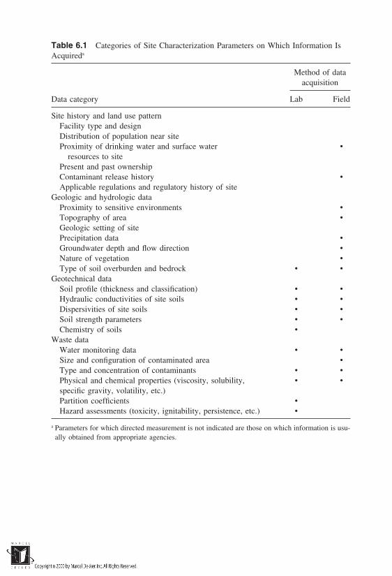
Table 6.1 Categories of Site Characterization Parameters on Which Information IsAcquireda

Method of dataacquisition

Data category Lab Field

Site history and land use patternFacility type and designDistribution of population near siteProximity of drinking water and surface water •

resources to sitePresent and past ownershipContaminant release history •Applicable regulations and regulatory history of site

Geologic and hydrologic dataProximity to sensitive environments •Topography of area •Geologic setting of sitePrecipitation data •Groundwater depth and flow direction •Nature of vegetation •Type of soil overburden and bedrock • •

Geotechnical dataSoil profile (thickness and classification) • •Hydraulic conductivities of site soils • •Dispersivities of site soils • •Soil strength parameters • •Chemistry of soils •

Waste dataWater monitoring data • •Size and configuration of contaminated area •Type and concentration of contaminants • •Physical and chemical properties (viscosity, solubility, • •specific gravity, volatility, etc.)Partition coefficients •Hazard assessments (toxicity, ignitability, persistence, etc.) •

a Parameters for which directed measurement is not indicated are those on which information is usu-ally obtained from appropriate agencies.

Table 6.2 Data Ranges and General Effects on Liquid Contaminant Migration froma Polluted Site

Increasing migration potentialFactor Units →

Release-specific parametersTime since last release Months Long Medium Short

(12) (1–12) (1)Site-specific parameters

Hydraulic conductivity cm-s Low Medium High(106) (105–103) (30)

Soil porosity % Low Medium High(19) (10–30) (30)

Soil surface area cm2g High Medium Low(50) (5–50) (5)

Liquid contaminant content % Low Medium High(10) (10–30) (30)

Soil temperature °C Low Medium High(10) (10–20) (20)

Rock fractures — Absent — PresentWater contenta % High Medium Low

(30) (10–30) (10)Contaminant-specific parameters

Liquid viscosity CP High Medium Low(20) (2–20) (2)

Liquid density g/cm3 Low Medium High(1) (1–2) (2)

a Although the referenced authors stated this, it is subject to debate.Source: Rosenberg et al. (1990).

Chemical sensing and geophysical techniques are increasingly being usedto delineate contaminated media without acquiring samples. In this section, focusis placed on techniques for contaminated zone delineation using soil sampling,groundwater sampling, and sensing techniques.

The stratigraphy of contaminated sites is the arrangement of beds of dif-ferent soils and rocks at a site. It may play a significant role in the rates anddirections of contaminant migration. Above the water table, it is usually conve-nient to sample soils and/or rocks for analyses. Analyses typically include con-taminant concentration measurements and geotechnical tests to measure flow-related characteristics such as particle size distribution, hydraulic conductivity,and fracture intensity. Several surface and bore-hole geophysical techniques sum-marized in Table 6.4 and 6.5, respectively, can be used for hydrogeological char-

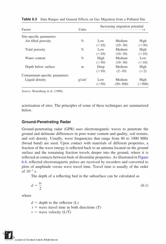
Table 6.3 Data Ranges and General Effects on Gas Migration from a Polluted Site

Increasing migration potentialFactor Units →

Site-specific parametersAir-filled porosity % Low Medium High

(10) (10–30) (30)Total porosity % Low Medium High

(10) (10–30) (10)Water content % High Medium Low

(30) (10–30) (10)Depth below surface m Deep Medium High

(10) (2–10) (2)Contaminant-specific parameters

Liquid density g/cm3 Low Medium High(50) (50–500) (500)

Source: Rosenberg et al. (1990).

acterization of sites. The principles of some of these techniques are summarizedbelow.

Ground-Penetrating Radar

Ground-penetrating radar (GPR) uses electromagnetic waves to penetrate theground and delineate differences in pore-water content and quality, soil texture,and soil density. Usually, wave frequencies that range from 80 to 1000 MHz(broad band) are used. Upon contact with materials of different properties, afraction of the wave energy is reflected back to an antenna located on the groundsurface and the remaining fraction travels deeper into the ground, where it isreflected at contacts between beds of dissimilar properties. As illustrated in Figure6.4, reflected electromagnetic pulses are received by recorders and converted toplots of amplitude versus wave travel time. Travel time is usually of the orderof 109 s.

The depth of a reflecting bed in the subsurface can be calculated as

d tv

2(6.1)

where

d depth to the reflector (L)t wave travel time in both directions (T)v wave velocity (L/T)

Table 6.4 Principal Surface Geophysical Techniques and Their Applications

Surface geophysicalsurvey method Applications Advantages Limitations

Seismic Refraction andReflection

Determines lithological Groundwater resource evaluations Relatively easy accessibility Resolution can be obscured in layeredchanges in subsur- Geotechnical profiling High depth of penetration depen- sequencesface Subsurface stratigraphic profiling dent on source of vibration Susceptibility to noise from urban

including top of bedrock Rapid areal coverage developmentDifficult penetration in cold weather

(depending on instrumentation)Operation restricted during wet weather

Electrical resistivityDelineates subsurface Depth to water table estimates Rapid areal coverage Susceptibility to natural and artificial

resistivity contrasts Subsurface stratigraphic profiling High depth of penetration electrical interferencedue to lithology, Groundwater resource evaluations possible (400–800 ft) Limited use in wet weathergroundwater, and High ionic strength contaminated High mobility Limited utility in urban areaschanges in ground- groundwater studies Results can be approximated Interpretation that assumes a layeredwater qualtiy in the field subsurface

Lateral heterogeneity not easily accountedfor

Ground-penetrating radarProvides continuous vi- Locating buried objects Great areal coverage Limited depth of penetration (a meter or

sual profile of shal- Delineation of bedrock subsurface High vertical resolution in suit- less in wet, clayey soils; up to 25 mlow subsurface ob- and structure able terrain in dry, sandy soils)jects, structure, and Delineation of karst features Visual picture of data Accessibility limited due to bulkiness oflithology Delineation of physical integrity of equipment and nature of survey

man-made earthen structures Interpretation of data qualitativeLimited use in wet weather

MagneticsDetects presence of Location of buried ferrous objects High mobility Detection dependent on size and ferrous

buried metallic ob- Detection of boundaries of landfills Data resolution possible in field content of buried objectjects containing ferrous objects Rapid areal coverage Difficult data resolution in urban areas

Location of iron-bearing rock Limited use in wet weatherData interpretation complicated in areas of

natural magnetic drift.

Source: Adapted from U.S. EPA (1991) and O’Brien and Gere Engineers (1988).

Table 6.5 Summary of Important Site Characterization Parameters and Bore-Hole Techniques for Their Measurement

Required information on the properties of rocks, fluid, wells, or thegroundwater system Widely available logging techniques that might be utilized

Lithology and stratigraphic correlation of aquifers and associated rocks Electric, sonic, or caliper logs made in open holes; nuclear logs made inopen or cased holes

Total porosity or bulk density or gamma-gamma Calibrated sonic logs in open holes, calibrated neutron logs in open orcased holes

Effective porosity or true resistivity Calibrated long-normal resistivity logsClay or shale content Gamma logsPermeability No direct measurement by logging; may be related to porosity, injectivity,

sonic amplitudeSecondary permeability—fractures, solution openings Caliper, sonic, or bore-hole televiewer or television logsSpecific yield of unconfined aquifers Calibrated neutron logsGrain size Possible relation to formation factor derived from electric logsLocation of water level or saturated zones Electric, temperature, or fluid conductivity in open hole or inside casing;

neutron or gamma-gamma logs in open hole or outside casingMoisture content Calibrated neutron logsInfiltration Time-interval neutron logs under special circumstances or radioactive

tracersDirection, velocity, and path of groundwater flow Single-well tracer techniques—point dilution and single-well pulse;

multiwell tracer techniquesDispersion, dilution, and movement of waste Fluid conductivity and temperature logs, gamma logs for some radioactive

wastes, fluid samplerSource and movement of water in a well Injectivity profile; flowmeter or tracer logging during pumping or injec-

tion; temperature logsChemical and physical characteristics of water, including salinity, tempera- Calibrated fluid conductivity and temperature in the well; neutron chloride

ture, density, and viscosity logging outside casing; multielectrode resistivityDetermining construction of existing wells, diameter and position of cas- Gamma-gamma, caliper, collar, and perforation locator, bore-hole tele-

ing, perforations, screens visionGuide to screen setting All logs providing data on the lithology, water-bearing characteristics, and

correlation and thickness of aquifersCementing Caliper, temperature, gamma-gamma; acoustic for cement bondCasing corrosion Under some conditions, caliper or collar locatorCasing leaks and/or plugged screen Tracer and flowmeter

Source: (Adapted from U.S. EPA (1991) and Keys and MacCary 1971).

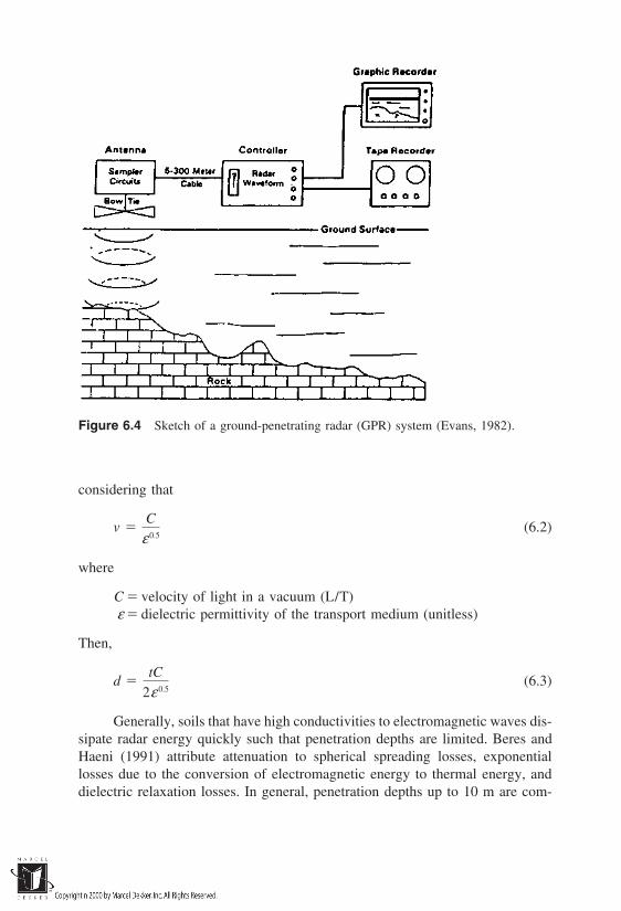
Figure 6.4 Sketch of a ground-penetrating radar (GPR) system (Evans, 1982).

considering that

v C

ε 0.5(6.2)

where

C velocity of light in a vacuum (L/T)ε dielectric permittivity of the transport medium (unitless)

Then,

d tC

2ε 0.5(6.3)

Generally, soils that have high conductivities to electromagnetic waves dis-sipate radar energy quickly such that penetration depths are limited. Beres andHaeni (1991) attribute attenuation to spherical spreading losses, exponentiallosses due to the conversion of electromagnetic energy to thermal energy, anddielectric relaxation losses. In general, penetration depths up to 10 m are com-

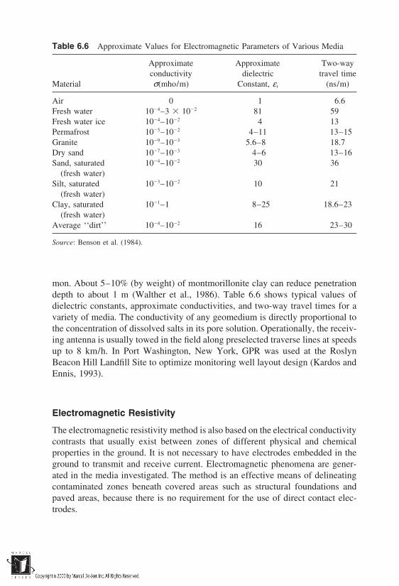
Table 6.6 Approximate Values for Electromagnetic Parameters of Various Media

Approximate Approximate Two-wayconductivity dielectric travel time

Material σ(mho/m) Constant, ε r (ns/m)

Air 0 1 6.6Fresh water 104–3 102 81 59Fresh water ice 104–102 4 13Permafrost 105–102 4–11 13–15Granite 109–103 5.6–8 18.7Dry sand 107–103 4–6 13–16Sand, saturated 104–102 30 36

(fresh water)Silt, saturated 103–102 10 21

(fresh water)Clay, saturated 101–1 8–25 18.6–23

(fresh water)Average ‘‘dirt’’ 104–102 16 23–30

Source: Benson et al. (1984).

mon. About 5–10% (by weight) of montmorillonite clay can reduce penetrationdepth to about 1 m (Walther et al., 1986). Table 6.6 shows typical values ofdielectric constants, approximate conductivities, and two-way travel times for avariety of media. The conductivity of any geomedium is directly proportional tothe concentration of dissolved salts in its pore solution. Operationally, the receiv-ing antenna is usually towed in the field along preselected traverse lines at speedsup to 8 km/h. In Port Washington, New York, GPR was used at the RoslynBeacon Hill Landfill Site to optimize monitoring well layout design (Kardos andEnnis, 1993).

Electromagnetic Resistivity

The electromagnetic resistivity method is also based on the electrical conductivitycontrasts that usually exist between zones of different physical and chemicalproperties in the ground. It is not necessary to have electrodes embedded in theground to transmit and receive current. Electromagnetic phenomena are gener-ated in the media investigated. The method is an effective means of delineatingcontaminated zones beneath covered areas such as structural foundations andpaved areas, because there is no requirement for the use of direct contact elec-trodes.

The principle of inducement of an electromagnetic field in geomedia forresistivity measurements is illustrated in Figure 6.5. A transmitter coil is heldor fixed on or close to the ground surface. An alternating current is applied tothe terminals of the coil to induce the flow of a current. This phenomenon gener-ates an alternating magnetic field, which in turn causes electric currents to perme-ate the earth. Within the earth, a secondary magnetic field is induced. The second-ary and primary magnetic fields are detected by a receiving coil placed nearthe transmitting coil. For a fixed intercoil spacing and operating frequency, themagnitude of the secondary magnetic field (or ratio of the secondary to primarymagnetic fields) is directly proportional to the conductivity of the ground. Resisti-vity can be computed from conductivity data. In a geomedium, the solid particlesact as insulators while soil moisture acts largely as a conductor of the electriccurrent. Furthermore, the conductivity of the pore fluid is proportional to theconcentration of ions within the fluid. Thus, these measurements can be used todelineate contaminated zones around waste containment barriers. If metallic ob-jects are present near the surveyed site, the readings recorded may be negativelyaffected. The effective depth of penetration can be as high as 60 m. This methodis often called the frequency domain electromagnetic (FDEM) method.

There are several variations of the electromagnetic induction method. Thedecay rate of magnetic field after the transmission is turned off can be measured.An eddy current flows through the ground at successively greater depths. Thedata obtained are interpreted to obtain resistivity variation with depth. This iscalled time domain electromagnetic (TDEM) survey. It has been applied byHoekstra et al. (1992) to trace the migration of brines from an oilfield brine pitin southwestern Texas. Penetration depths of up to 500 m are estimated by Hoeks-tra et al. (1992). Another type of (EM) measurement involves the use of verylow frequencies (15–25 kHz). In this method, ground contact is required for

Figure 6.5 Induced electromagnetic fields (McNeil, 1982).

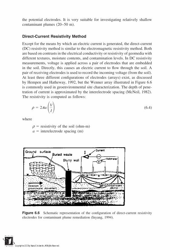
the potential electrodes. It is very suitable for investigating relatively shallowcontaminant plumes (20–50 m).

Direct-Current Resistivity Method

Except for the means by which an electric current is generated, the direct-current(DC) resistivity method is similar to the electromagnetic resistivity method. Bothare based on contrasts in the electrical conductivity or resistivity of geomedia withdifferent textures, moisture contents, and contamination levels. In DC resistivitymeasurements, voltage is applied across a pair of electrodes that are embeddedin the soil. Directly, this causes an electric current to flow through the soil. Apair of receiving electrodes is used to record the incoming voltage (from the soil).At least three different configurations of electrodes (arrays) exist, as discussedby Hempen and Hatheway, 1992, but the Wenner array illustrated in Figure 6.6is commonly used in geoenvironmental site characterization. The depth of pene-tration of current is approximated by the interelectrode spacing (McNeil, 1982).The resistivity is computed as follows:

ρ 2πa V

I (6.4)

where

ρ resistivity of the soil (ohm-m)a interelectrode spacing (m)

Figure 6.6 Schematic representation of the configuration of direct-current resistivityelectrodes for contaminant plume remediation (Inyang, 1994).

I current flow through outer electrodes (A)V voltage across inner electrodes (V)

The relationship between the physicochemical and textural characteris-tics of a medium and its resistivity is represented by Archie’s law. It is given as

ρ ρw

φ µS2(6.5)

where

ρ resistivity of the geomediumρw resistivity of water in the mediumφ porosity of the mediumµ cementation constant of the medium 1.3 for consolidated

sandsS degree of saturation of the medium with water

Figure 6.7 (Rhoades and Halvorson, 1977) shows the relationship be-tween electrode configuration and the area monitored. The flowchart of resistivitymeasurements and data analysis steps is shown in Figure 6.8 (Nielson, 1991).Vertical resistivities of horizontally bedded media are represented by ρ1, ρ2, ρ3,and ρ4.

For any four-electrode configuration such as the Werner system, two cate-gories of measurements can be conducted:

Sounding: The electrodes that transmit current are placed at increasing dis-tances apart and measurements are made. Deeper parts of a geomediumare investigated using wider spacings.

Profiling: The entire array is moved from one location to another using thesame electrode spacing. This provides an opportunity to assess lateralvariations in electrical resistivity of media.

At contaminated sites, both lateral and vertical variabilities in geochemistryare often found. As shown in Figure 6.9, a geoelectrical soil profile that is concep-tually stratified in terms of electrical resistivity may be considered for the purposeof estimating a composite value of resistivity. Dar Zarrouk parameters configuredby Maillet (1947) as presented below are used for this purpose. Following thetreatment by van Zijl (1978) in conjunction with Figure 6.9,

T n1

i1

ρihi (6.6)

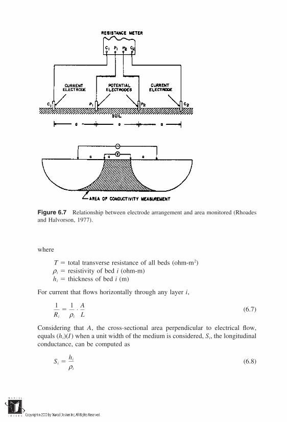
Figure 6.7 Relationship between electrode arrangement and area monitored (Rhoadesand Halvorson, 1977).

where

T total transverse resistance of all beds (ohm-m2)ρ i resistivity of bed i (ohm-m)hi thickness of bed i (m)

For current that flows horizontally through any layer i,

1Ri

1ρi

⋅ A

L(6.7)

Considering that A, the cross-sectional area perpendicular to electrical flow,equals (hi)(I ) when a unit width of the medium is considered, Si, the longitudinalconductance, can be computed as

Si hi

ρi

(6.8)

Figure 6.8 Flowchart of resistivity measurement and data analysis steps (Nielson,1991).

and for all beds,

S n1

i1

hi

ρi

(6.9)

where S total longitudinal conductance (siemens).The average transverse resistivity and average longitudinal resistivity can

be computed using Eqs. (6.10) and (6.11), respectively:

ρa T

H

∑ hρ∑ h

(6.10)

ρL H

S

∑ h

∑ h/p(6.11)

If a geomedium of very high vertical variability in electrical properties is evalu-ated, its anisotropy can be expressed as

Figure 6.9 Schematic representation of a geoelectrical section for composite apparentresistivity analysis (van Zijl, 1978).

λ √ρa

ρL

√TS

H 2(6.12)

For practical purposes, it may be convenient to consider the entire section ashaving a resistivity value ρc that may be estimated as in Eq. (6.13):

ρc √ρaρL (6.13)

Then

T λH ⋅ ρc (6.14)

S λH

ρc

(6.15)

and

ρc √T

S λρL (6.16)

Figure 6.10 Typical ranges of resistivity data for various geomedia (Nielsen, 1991).

Figure 6.10 and Table 6.7 show typical ranges of resistivities of aqueousand geological media.

Seismic Methods

Seismic methods are useful for assessment of the structural characteristics of acontaminated site. They are not suitable for use in contaminated zone delineationbecause contaminants do not exhibit sufficient variations in their responses toseismic waves. Elastic waves generated by seismic sources travel faster in dense,tightly cemented and wet materials than in loose dry materials, hence seismicwave velocity is directly proportional to the density of the transport medium.This principle can be applied to the identification of potential migration pathwaysfor contaminants in the subsurface. Equations (6.17), (6.18), and (6.19) show therelationships between seismic wave velocities and geological properties.

Vp k

ρ0.5

(6.17)

Vp 4µ/3ρ

0.5

(6.18)

Vs µρ

0.5

(6.19)

Table 6.7 Typical Ranges of Resistivity Data for VariousAqueous and Geological Media

ResistivityEarth materiala (Ω-m)

Saline groundwater 0.01–1Clay soil 1–30Fresh groundwater 2–50Calcareous shale (or chalk) 10–100Sand (SP, moderately to highly saturated) 20–200Shale (mudstone/claystone) 1–500Shale (siltstone) 50–1,000Limestone (low-density) 100–1,000Volcanic flow rock (scoriaceous basalt) 300–1,000Lodgement (dense, clayey, basal) till 50–5,000Sandstone, uncemented 30–10,000Ablation (dry, loose, chsionless) till 1,000–10,000Fluvial sands and gravels (GW, unsaturated) 1,000–10,000Loose, poorly sorted sand (SP, unsaturated) 1,000–100,000Metamorphic rock 50–1,000,000Crystalline igneous rock 100–1,000,000Limestone (high-density) 1,000–1,000,000

a GW and SP are Unified Soil Classification terms for well-graded gravel andpoorly graded sand, respectively.

Source: Hempen and Hatheway (1992).

where

Vp compressional wave velocity (L/T)Vs shear wave velocity (L/T)k bulk modulus of the mediumµ shear modulus of the mediumρ density of the medium (M/L3)

Table 6.8 (Hempen and Hatheway, 1992) and Figure 6.11 (Nielsen, 1991)show typical seismic wave velocity ranges for geomedia. Surface refractionmethod has utility in the delineation of bedrock boundaries at contaminated sites.It is generally effective within a depth range of about 30 m. The operating princi-ple of this method is that compressional waves are bent at the interface betweenmedia of significantly different physical characteristics. Among such characteris-tics are elasticity, density, and other parameters which can be correlated withthem such as porosity and degree of cementation. Usually, a hammer hit or dropweight is used to generate waves in the case of shallow investigations at waste

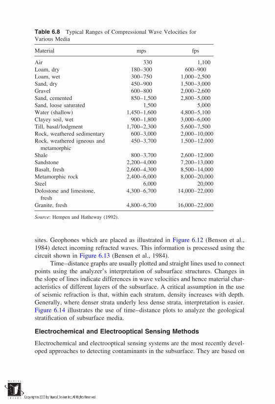
Table 6.8 Typical Ranges of Compressional Wave Velocities forVarious Media

Material mps fps

Air 330 1,100Loam, dry 180–300 600–900Loam, wet 300–750 1,000–2,500Sand, dry 450–900 1,500–3,000Gravel 600–800 2,000–2,600Sand, cemented 850–1,500 2,800–5,000Sand, loose saturated 1,500 5,000Water (shallow) 1,450–1,600 4,800–5,100Clayey soil, wet 900–1,800 3,000–6,000Till, basal/lodgment 1,700–2,300 5,600–7,500Rock, weathered sedimentary 600–3,000 2,000–10,000Rock, weathered igneous and 450–3,700 1,500–12,000

metamorphicShale 800–3,700 2,600–12,000Sandstone 2,200–4,000 7,200–13,000Basalt, fresh 2,600–4,300 8,500–14,000Metamorphic rock 2,400–6,000 8,000–20,000Steel 6,000 20,000Dolostone and limestone, 4,300–6,700 14,000–22,000

freshGranite, fresh 4,800–6,700 16,000–22,000

Source: Hempen and Hatheway (1992).

sites. Geophones which are placed as illustrated in Figure 6.12 (Benson et al.,1984) detect incoming refracted waves. This information is processed using thecircuit shown in Figure 6.13 (Bensen et al., 1984).

Time–distance graphs are usually plotted and straight lines used to connectpoints using the analyzer’s interpretation of subsurface structures. Changes inthe slope of lines indicate differences in wave velocities and hence material char-acteristics of different layers of the subsurface. A critical assumption in the useof seismic refraction is that, within each stratum, density increases with depth.Generally, where denser strata underly less dense strata, interpretation is easier.Figure 6.14 illustrates the use of time–distance plots to analyze the geologicalstratification of subsurface media.

Electrochemical and Electrooptical Sensing Methods

Electrochemical and electrooptical sensing systems are the most recently devel-oped approaches to detecting contaminants in the subsurface. They are based on

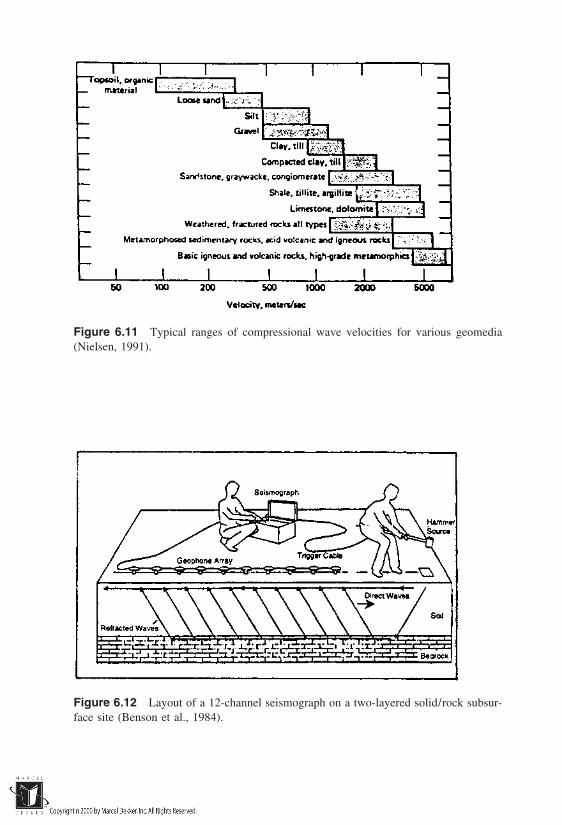
Figure 6.11 Typical ranges of compressional wave velocities for various geomedia(Nielsen, 1991).

Figure 6.12 Layout of a 12-channel seismograph on a two-layered solid/rock subsur-face site (Benson et al., 1984).

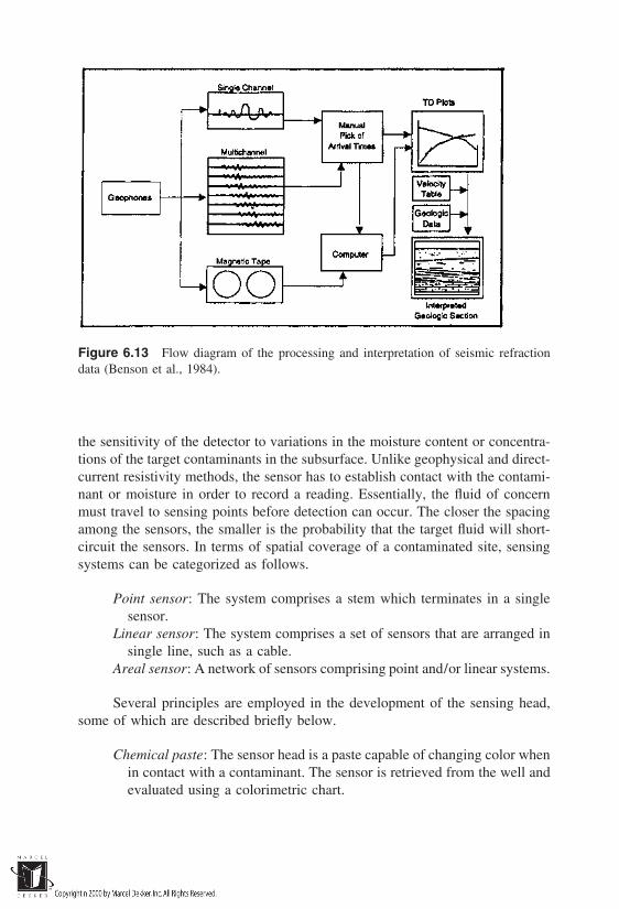
Figure 6.13 Flow diagram of the processing and interpretation of seismic refractiondata (Benson et al., 1984).

the sensitivity of the detector to variations in the moisture content or concentra-tions of the target contaminants in the subsurface. Unlike geophysical and direct-current resistivity methods, the sensor has to establish contact with the contami-nant or moisture in order to record a reading. Essentially, the fluid of concernmust travel to sensing points before detection can occur. The closer the spacingamong the sensors, the smaller is the probability that the target fluid will short-circuit the sensors. In terms of spatial coverage of a contaminated site, sensingsystems can be categorized as follows.

Point sensor: The system comprises a stem which terminates in a singlesensor.

Linear sensor: The system comprises a set of sensors that are arranged insingle line, such as a cable.

Areal sensor: A network of sensors comprising point and/or linear systems.

Several principles are employed in the development of the sensing head,some of which are described briefly below.

Chemical paste: The sensor head is a paste capable of changing color whenin contact with a contaminant. The sensor is retrieved from the well andevaluated using a colorimetric chart.

Figure 6.14 Illustration of the effects of subsurface stratification on obtained seismicvelocity (v) plots for a buried dense ridge (top) and a dense ledge (bottom) (Henbest etal., 1971).

Permeable coating: The coating repels water and some contaminants, butis permeable by others which activate a signal upon entry into the sensinghead.

Photo ionization: Molecules of gases emitted from contaminants are ion-ized when they absorb ultraviolet light. The ionization parameters arescaled against concentration. Inyang et al. (1992) have described theprinciple of photoionization and its application to hydrocarbon vapordetection. Generally,

R hν ⇒ R e (6.20)

where

R the species prior to ionizationhν photon with energy in excess of the species ionization potentialR ionized speciese released electron

Generally, photon energies of the order of 10.2 eV are used for compounds thatmay be present in petroleum-contaminated media.

Fiber-optic sensing: These sensors are based on the transmission of probesignals within the visible light regime by optical fibers through very longdistances to embedded sensors. Wavelength-dependent optical attenua-tion of the probe beam or production of fluorescent emissions by thecontaminant is measured and scaled as an index of the presence of thecontaminant. Often, an organic dye is added to the sensor to promotefluorescence upon reaction with low concentrations of the target com-pound. Most of the relevant reactions are reversible, making it possibleto sense new contaminant concentration levels. In general, the Beer-Lambert law can be applied to the optical absorbency of the detectedcompounds.

Ic I0 exp[a(λ,pH)Cd ] (6.21)

where

Ic transmitted light intensity due to the presence of thecontaminant

I0 light source intensitya molar absorptivity of the compoundλ selected wavelengthd optical path lengthC velocity of light

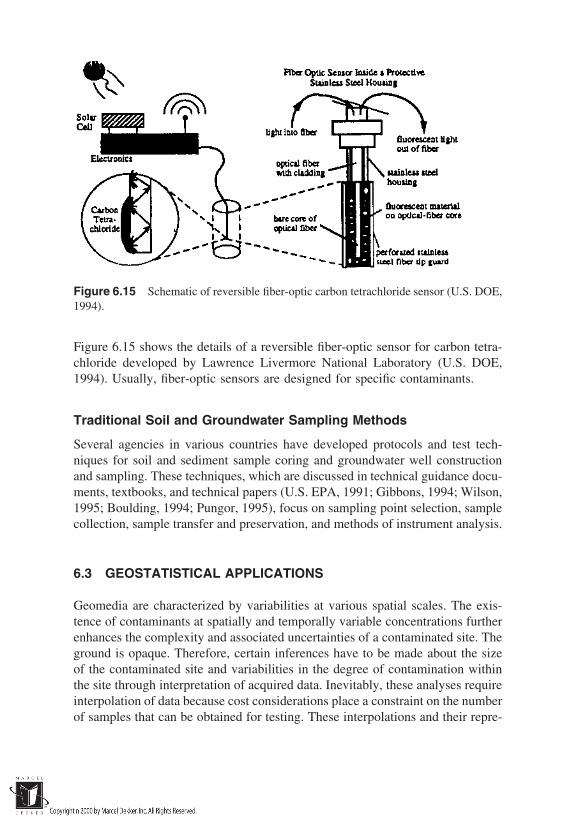
Figure 6.15 Schematic of reversible fiber-optic carbon tetrachloride sensor (U.S. DOE,1994).

Figure 6.15 shows the details of a reversible fiber-optic sensor for carbon tetra-chloride developed by Lawrence Livermore National Laboratory (U.S. DOE,1994). Usually, fiber-optic sensors are designed for specific contaminants.

Traditional Soil and Groundwater Sampling Methods

Several agencies in various countries have developed protocols and test tech-niques for soil and sediment sample coring and groundwater well constructionand sampling. These techniques, which are discussed in technical guidance docu-ments, textbooks, and technical papers (U.S. EPA, 1991; Gibbons, 1994; Wilson,1995; Boulding, 1994; Pungor, 1995), focus on sampling point selection, samplecollection, sample transfer and preservation, and methods of instrument analysis.

6.3 GEOSTATISTICAL APPLICATIONS

Geomedia are characterized by variabilities at various spatial scales. The exis-tence of contaminants at spatially and temporally variable concentrations furtherenhances the complexity and associated uncertainties of a contaminated site. Theground is opaque. Therefore, certain inferences have to be made about the sizeof the contaminated site and variabilities in the degree of contamination withinthe site through interpretation of acquired data. Inevitably, these analyses requireinterpolation of data because cost considerations place a constraint on the numberof samples that can be obtained for testing. These interpolations and their repre-

sentation through contouring of concentrations may be a requirement for the se-lection and design of potentially effective remediation schemes. Uncertaintiesabout the nature of the contamination at a site can be minimized through theapplication of geostatistical techniques to sampling design and analysis.

6.3.1 Spatial Distribution of Monitoring Points

Monitoring points should be distributed such that contaminant concentrationsand hydrogeological parameters can be estimated for the entire three-dimensionalspace using measurements at the selected points. It is desirable that monitoringnetwork design be such that biases in the interface about hydrogeological andcontamination scenarios at the site are minimal. Two important geostatistical pa-rameters are critical with respect to monitoring point distribution.

Sampling pattern: This is the geometric configuration of monitoring pointsin three-dimensional space. Often, more emphasis is placed on the arealdistribution of projections of monitoring points on the ground surface.

Sampling density: This is the number of sampling points per space unit.The space unit could be a unit area or a unit volume of the sampledgeomedia.

Figure 6.16 shows various types of monitoring networks with descriptionsof their utilities as described by the U.S. EPA (1991) and by Gilbert (1987). Ingeneral, samples may be taken along transects (lines) from within grids. Somegeneral knowledge or informed suspicion about the hydrogeological conditionsof a site is necessary for the selection of an effective monitoring network. Thesource of such information could be reconnaissance surveys and/or historicalrecords as outlined in Table 6.1.

Sampling point density is another critical determinant of sampling effi-ciency. For a given network, sampling efficiency is directly proportional to sam-pling point density. Olea (1984) estimates that the efficiency of the network witha higher density relates to that of the lower density in consistence with Eq. (6.22):

∆E Eh EL DL

Dh

0.5

(6.22)

where

∆E difference between sampling efficiencies of two networksEh sampling efficiency of the higher-density networkEL sampling efficiency of the lower-density networkDL lower sampling point density (number/space unit)Dh higher sampling point density (number/space unit)

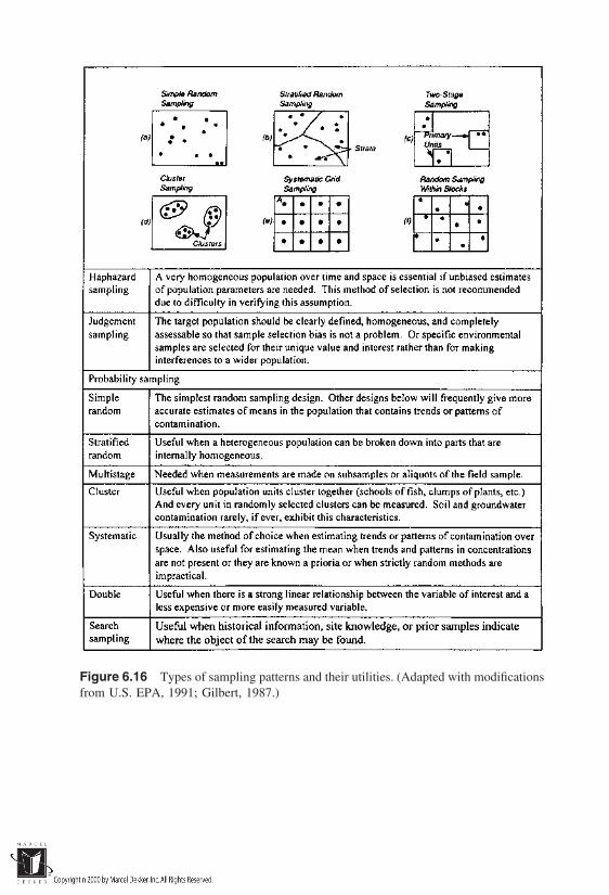
Figure 6.16 Types of sampling patterns and their utilities. (Adapted with modificationsfrom U.S. EPA, 1991; Gilbert, 1987.)

6.3.2 Contaminated Zone Contouring UsingMeasured Data

One of the most useful geostatistical techniques for contouring of spatially vari-able site characteristics data is kriging. This is a method of estimating the magni-tudes of parameters for a network of points given measurements on points thatdo not necessarily coincide with the network points. In essence, kriging is a formof spatial interpolation which is useful for contouring of geostatistical data.

As represented in Figure 6.17, Z0 is an unknown value of a parameter tobe estimated from measured values Z1, Z2, Z3. For the two-dimensional case,C1xy, C2xy, and C3xy are designated as corresponding coordinates. Similarly, thecoordinates of Z0 can be designated as C0xy. Each of the measured values contrib-utes to Z*0 , the estimated value of Z0. The general kriging equation can be writ-ten as

Z*0 n

i1

λ iZi (6.23)

n

i1

λ i (6.24)

where

Z*0 estimated magnitude of unmeasured parameter at interpolationlocation C0xy

Zi measured values of the parameter at locations that surroundC0xy: locations such as C1xy and C2xy

λ i weight of the kriging estimator

The weighting factors can be developed by direct correlation with distancesof measurement points from C0xy. Additional information on kriging techniquesis provided by de Marsily (1986), Journel (1989), and Jury (1986).

Figure 6.17 Illustration of the use of measured data for spatial interpolation.

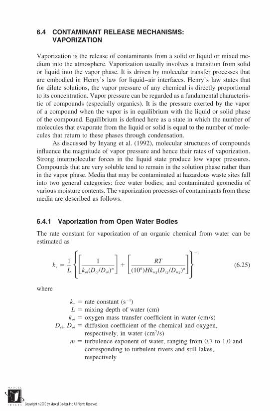
6.4 CONTAMINANT RELEASE MECHANISMS:VAPORIZATION

Vaporization is the release of contaminants from a solid or liquid or mixed me-dium into the atmosphere. Vaporization usually involves a transition from solidor liquid into the vapor phase. It is driven by molecular transfer processes thatare embodied in Henry’s law for liquid–air interfaces. Henry’s law states thatfor dilute solutions, the vapor pressure of any chemical is directly proportionalto its concentration. Vapor pressure can be regarded as a fundamental characteris-tic of compounds (especially organics). It is the pressure exerted by the vaporof a compound when the vapor is in equilibrium with the liquid or solid phaseof the compound. Equilibrium is defined here as a state in which the number ofmolecules that evaporate from the liquid or solid is equal to the number of mole-cules that return to these phases through condensation.

As discussed by Inyang et al. (1992), molecular structures of compoundsinfluence the magnitude of vapor pressure and hence their rates of vaporization.Strong intermolecular forces in the liquid state produce low vapor pressures.Compounds that are very soluble tend to remain in the solution phase rather thanin the vapor phase. Media that may be contaminated at hazardous waste sites fallinto two general categories: free water bodies; and contaminated geomedia ofvarious moisture contents. The vaporization processes of contaminants from thesemedia are described as follows.

6.4.1 Vaporization from Open Water Bodies

The rate constant for vaporization of an organic chemical from water can beestimated as

kv 1L 1

koi(Dci/Doi)m RT

(106)Hkwg(Dcg/Dwg)n1

(6.25)

where

kv rate constant (s1)L mixing depth of water (cm)

koi oxygen mass transfer coefficient in water (cm/s)Dci, Doi diffusion coefficient of the chemical and oxygen,

respectively, in water (cm2/s)m turbulence exponent of water, ranging from 0.7 to 1.0 and

corresponding to turbulent rivers and still lakes,respectively

R ideal gas constant (see below)T temperature (K)H Henry’s law constant (atm-m3/mol)

kwg mass transfer coefficient of water vapor in air (0.58cm/s)

Dcg, Dwg diffusion coefficient of the chemical and water,respectively, in air (cm2/s)

n gas turbulence exponent, ranging from 0.5 to 1.0

Usually the quantity RT is combined such that it approximates 2.40 102

atm-m3/mol. As discussed by the U.S. EPA (1988), Dcg can be estimated as fol-lows if measured data are unavailable:

Dcg 0.0067 T1.5(0.034 M1)0.5 M0.17[(M/2.5d )0.33 1.81]2 (6.26)

where

M molecular weight of the chemical compound (g/g-mol)d density of the liquid (g/cm3)

Values of kv computed through the use of Eq. (6.25) can be introduced intoEq. (6.27) to obtain the half-life of the vaporizing chemical compound. The half-life is the time it takes for half the original quantity of the substance to vaporize:

t0.5 ln2kv

0.693

kv

(6.27)

Equation (6.27) is applicable to a situation in which the vaporization process ofthe compound is of the first order. For a second-order process,

t0.5 1

k′vC0

(6.28)

where

k′v second-order vaporization rate constant (L3/MT)C0 initial concentration of the vaporizing substance (M/L3)

For impoundments and other quiescent water masses of fluids such as thoseillustrated in Figures 6.1D and 6.1H, the rate of emissions of contaminants intothe atmosphere is obtainable from

Er kcAeCL (6.29)

where

Er rate of emissions from the surface of the liquid (M/T)kc composite mass transfer coefficient (M/T)

Ae exposed surface area of the liquid (L2)CL concentration of the vaporizing constituent in the liquid (M/L3)

Essentially, kc is a function of the mass transfer coefficients of the liquidand gas phases and Henry’s law constant. Using specific units,

1kc

1kL

1

kGke

(6.30)

where

kc composite mass transfer coefficient (m/s)kL liquid-phase mass transfer coefficient (m/s)kG gas-phase mass transfer coefficient (m/s)ke equilibrium constant or partition coefficient that represents the

ratio of the chemical’s concentration in the gas phase to that inthe liquid phase (dimensionless)

Here ke is a function of Henry’s law constant as follows:

ke H

RT(6.31)

where

H Henry’s law constant (atm-m3/mol)R universal gas constant 8.21 105 atm-m3/mol-KT temperature (K)

If vaporization occurs at the standard environmental temperature of 25°C, Eq.(6.31) can be written as

ke (40.9)H (6.32)

Values of H for a variety of chemical compounds are obtainable from standardchemistry and chemical engineering texts. Generally, H can be estimated as theratio of vapor pressure (expressed in atm) to aqueous solubility (expressed inmol/m3) of the chemical concerned. Values of Henry’s law constant for someorganic compounds are presented in Table 6.9.

Huang (1982) has provided a comprehensive review of volatile emissionsfrom waste management facilities.

6.4.2 Vaporization from Geomedia

The site contamination scenarios represented by Figures 6.1B, 6.1D, 6.1F, 6.1G,and 6.1H illustrate situations in which volatile contaminants can be emitted fromgeomedia. In contrast to open water bodies and impoundments, the presence of

soil and rock particles affects both the vaporization and transport processes ofchemical compounds into the open atmosphere. For example, as explained byInyang et al. (1992), the solution phase is not spatially continuous in a moistsoil, but is smeared on soil grains. Consequently, capillary forces may influencethe vapor pressures and hence the vaporization rates of volatile contaminants.Barrow (1961) developed some numerical relationships for estimating reductionsin vapor pressures of chemicals due to fluid surface curvature induced by thepresence of soil particles. The reader is referred to that textbook.

For a soil contamination case in which gas adsorption by soil particles,depletion rate effects of the vaporizing substances, and internal gas generationprocesses exemplified by biodegradation are ignored, Fick’s first law of steady-state diffusion can be applied to develop expressions for the emission rates ofcontaminants from buried or exposed waste. Emission is considered to occur ata horizontal plane coincident with the ground surface, and contaminant immedi-ately above the ground surface is zero. With these largely conservative assump-tions, Farmer et al. (1978) developed emission equations which were subse-quently modified by Shen (1981) and Farino et al. (1983) in the following finalform:

Ei DiCsiAg(n4/3)Mi

de

(6.33)

where

Ei emission rate of contaminant i (M/T)Di diffusion coefficient of contaminant i in air (L2/T)Csi saturation vapor concentration of component i (M/L3)Ag exposed area on the ground surface (L2)n total porosity of the soil (dimensionless fraction)

Mi mole fraction of the toxic contaminant i in the waste (mole/mole)

de effective depth of the soil cover (L)

n 1 ρb

ρp (6.34)

Csi VpMi

RT(6.35)

where

ρb bulk density of soil (M/L3), which varies generally between 1and 2 g/cm3

ρp particle density of the soil (M/L3), which is typically about2.65 g/cm3

Table 6.9 Values of Henry’s Law Constants for Some Organic Compounds

Vapor Molecular H m3-atm/mol 103

pressure Temperature Solubility Temperature weightCompound (atm 103) (K) (g/m3) (K) (g/mol) Calculated Experimental

Acenaphthene — — 3.93 298 154.2 — 0.241Benzene 125 298 1,780 298 78.1 5.48 5.55Carbon tetrachloride 149 298 800 298 153.8 28.6 30.2Chlorobenzene 15.5 298 472 298 112.6 3.70 3.931,2,4-Trichlorobenzene 0.383 298 30 — 181.5 2.32 1.42Hexachlorobenzene — — 0.006 298 284.8 — 1.701,2-Dichloroethane 113 298 8,300 298 99.0 1.35 1.101,1,1-Trichloroethane 168 298 5,497 298 133.4 4.08 4.92Hexachloroethane — — 50 295 236.7 — 9.831,1-Dichloroethane 3.8 298 5,500 293 99.0 5.54 5.45Chloroform 260 298 9,600 298 119.2 3.23 3.391,2-Dichlorobenzene 1.97 298 145 298 147.0 2.00 1.941,3-Dichlorobenzene 2.48 298 123 298 147.0 2.96 2.631,4-Dichlorobenzene — — 79 298 147.0 — 2.721,1-Dichloroethylene 778 298 5,000 293 97.0 15.1 15.01,2-trans-Dichloroethylene 263 287 6,300 293 96.9 4.05 5.321,2-Dichloropropane 65.8 298 2,700 293 113.0 2.75 2.82

1,3-Dichloropropylene 32.9 293 2,700 298 111.0 1.35 3.55Ethylbenzene 12.5 298 206 298 106.2 6.44 6.44Methylene chloride 599a 298 16,700 298 84.9 3.04 3.19Bromoform 7.37 298 3,130 298 252.8 0.595 0.532Bromodichloromethane — — — — 163.8 — 2.12Trichlorofluoromethane 833 298 1,100 298 137.4 104 58.3Dibromochloromethane 65.8 293 — — 168.8 — 0.783Hexachlorobutadiene 0.197 293 2 293 260.8 25.7 10.3Hexachlorocyclopentadiene 0.107 298 0.805 298 272.7 36.5 16.4Nitrobenzene 0.374 298 2,000 298 123.1 0.023 0.0244,6-Dinitro-o-cresol — — — — 198.1 — 0.0014Phenol — — 67,000 298 94.1 — 0.0013Acenaphthylene — — 3.93 298 152.2 — 0.114Fluorene — — 1.98 298 116.2 — 0.117Tetrachloroethylene 25.8a 298 150 298 165.8 28.5 28.7Toluene 37.4 298 535 298 92.1 6.44 5.93Trichloroethylene 97.8 298 1,100 298 131.5 11.7 11.7Aldrin — — 0.2 293 364.9 — 0.496Dieldrin — — 0.186 298 380.9 — 0.058

Source: Resummarized from Huang (1982).

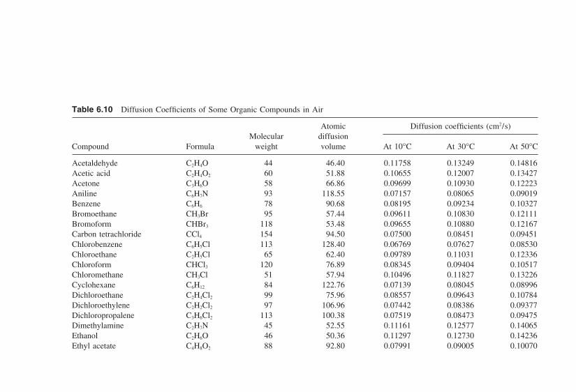
Table 6.10 Diffusion Coefficients of Some Organic Compounds in Air

Atomic Diffusion coefficients (cm2/s)Molecular diffusion

Compound Formula weight volume At 10°C At 30°C At 50°C

Acetaldehyde C2H4O 44 46.40 0.11758 0.13249 0.14816Acetic acid C2H4O2 60 51.88 0.10655 0.12007 0.13427Acetone C3H6O 58 66.86 0.09699 0.10930 0.12223Aniline C6H7N 93 118.55 0.07157 0.08065 0.09019Benzene C6H6 78 90.68 0.08195 0.09234 0.10327Bromoethane CH3Br 95 57.44 0.09611 0.10830 0.12111Bromoform CHBr3 118 53.48 0.09655 0.10880 0.12167Carbon tetrachloride CCl4 154 94.50 0.07500 0.08451 0.09451Chlorobenzene C6H5Cl 113 128.40 0.06769 0.07627 0.08530Chloroethane C2H5Cl 65 62.40 0.09789 0.11031 0.12336Chloroform CHCl3 120 76.89 0.08345 0.09404 0.10517Chloromethane CH3Cl 51 57.94 0.10496 0.11827 0.13226Cyclohexane C6H12 84 122.76 0.07139 0.08045 0.08996Dichloroethane C2H4Cl2 99 75.96 0.08557 0.09643 0.10784Dichloroethylene C2H2Cl2 97 106.96 0.07442 0.08386 0.09377Dichloropropalene C3H6Cl2 113 100.38 0.07519 0.08473 0.09475Dimethylamine C2H7N 45 52.55 0.11161 0.12577 0.14065Ethanol C2H6O 46 50.36 0.11297 0.12730 0.14236Ethyl acetate C4H8O2 88 92.80 0.07991 0.09005 0.10070

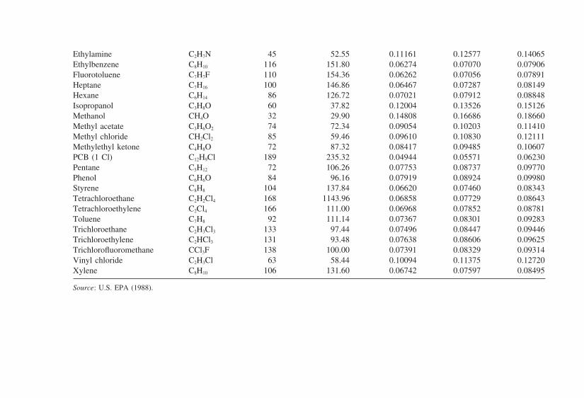
Ethylamine C2H7N 45 52.55 0.11161 0.12577 0.14065Ethylbenzene C8H10 116 151.80 0.06274 0.07070 0.07906Fluorotoluene C7H7F 110 154.36 0.06262 0.07056 0.07891Heptane C7H16 100 146.86 0.06467 0.07287 0.08149Hexane C6H14 86 126.72 0.07021 0.07912 0.08848Isopropanol C3H8O 60 37.82 0.12004 0.13526 0.15126Methanol CH4O 32 29.90 0.14808 0.16686 0.18660Methyl acetate C3H6O2 74 72.34 0.09054 0.10203 0.11410Methyl chloride CH2Cl2 85 59.46 0.09610 0.10830 0.12111Methylethyl ketone C4H8O 72 87.32 0.08417 0.09485 0.10607PCB (1 Cl) C12H9Cl 189 235.32 0.04944 0.05571 0.06230Pentane C5H12 72 106.26 0.07753 0.08737 0.09770Phenol C6H6O 84 96.16 0.07919 0.08924 0.09980Styrene C8H8 104 137.84 0.06620 0.07460 0.08343Tetrachloroethane C2H2Cl4 168 1143.96 0.06858 0.07729 0.08643Tetrachloroethylene C2Cl4 166 111.00 0.06968 0.07852 0.08781Toluene C7H8 92 111.14 0.07367 0.08301 0.09283Trichloroethane C2H3Cl3 133 97.44 0.07496 0.08447 0.09446Trichloroethylene C2HCl3 131 93.48 0.07638 0.08606 0.09625Trichlorofluoromethane CCl3F 138 100.00 0.07391 0.08329 0.09314Vinyl chloride C2H3Cl 63 58.44 0.10094 0.11375 0.12720Xylene C8H10 106 131.60 0.06742 0.07597 0.08495

Source: U.S. EPA (1988).

Vp vapor pressure of the chemical (mmHg)Mi molar weight of contaminant i (M/mole)R universal gas constant (62,361 mmHg-cm3/mol-K)T absolute temperature (K)

The diffusion coefficient, Di, of a contaminant in air can be estimated as

Di D′(M′/Mi)0.5 (6.36)

where

Di diffusion coefficient of the contaminant (L2/T)D′ known diffusion coefficient of a specific compound (L2/T)M′ molecular weight of the compound that had D′ (M)Mi molecular weight of the compound for which Di is being

estimated (M)

Values of Di for selected organic compounds are presented in Table 6.10.It should be noted that the presence of moisture in soil reduces the flow

rate of emitted gases by increasing the tortuosity of flow paths.

6.5 CONTAMINANT RELEASE MECHANISMS: DUSTING

Dusting is the removal of fine soil particles by mechanical action. Usually, humanactivities and wind are the agents of dusting. Fine dust particles are consideredto be pollutants due to their negative impacts on human health when inhaled andtheir hazard to plants. Both organic and inorganic contaminants may be presentin dust, especially if it is generated from contaminated media such as those illus-trated in Figures 6.1B, 6.1C, and 6.1E.

Cowherd et al. (1977) developed Eq. (6.37) for prediction of the averageannual suspended particulate emissions due to wind action on flat or rolling ter-rain:

E 3900(e/110)(s/15)( f/25)V

(Pi/50)2(6.37)

where

E emission rate of suspended particles smaller than 30 µm inStokes diameter (kg/ha-yr)

e surface erodibility or potential annual loss rate for a wide, openfield with erodible dry aggregates (20 mesh screen; kg/ha-yr)

s surface silt content [particles smaller than 75 µm (%)]f percent of time that the wind velocity at 30 cm above the dust

source exceeds the nominal wind erosion threshold of 5.4 m/s(%)

V fractional value that reflects the reducing effect of vegetation onwind erosion (1.0 for bare soil, and a fraction for vegetatedmedia)

Pi Thornthwaite’s precipitation-evaporation Index for averagemoisture content of the source media

The value 3900 kg/ha-yr is a proportionality constant that is based on measure-ments in west Texas.

The revolving action of automobile tires on the surface of terrain alsocauses the emission of fine particulate matter. There exists an aerodynamic wakeregion behind the moving vehicle in which dust particles are thrown upward intothe air. Dust particles that adhere to automobile tires can also be thrown up di-rectly. Empirical relationships are commonly used to estimate emission rates forvehicular action. Equation (6.38) is an example.

E 0.61(S/12)(Vh/48)(W/2.7)0.7(nw/4)0.5 [(365 p)/365] (6.38)

where

E emission rate (kg/vehicle-km-h)S silt content of the surface (%)

Vh mean vehicular speed (km/h)W mean vehicular weight (Mg)nw mean number of wheelsp number of days with precipitation 0.254 mm

6.6 CONTAMINANT RELEASE MECHANISMS: LEACHING

Leaching is the process by which chemical substances are removed from a matrixand transported to the boundaries of the releasing matrix. The removal processmay be dominated by dissolution of the chemical substance by the leaching solu-tion (leachant) or through the detachment of minute particles from the matrix.Thus the essential difference between leaching and dissolution is that the latterdoes not cover transport material to the boundary of the matrix while the formerdoes. Dissolution can be considered as one of the leaching phenomena. The trans-port involved in leaching is within the source matrix boundaries and should bedifferentiated from the contaminant fate and transport processes that occur afterthe leached constituents exit the matrix. Establishment of the physical boundaryfor the two categories of processes differentiated above is important from thestandpoint of contaminant emission rate computation.

The concentration of the target contaminant outside that boundary is animportant determinant of the leaching rate if the leaching process is diffusioncontrolled. This is attributable to the fact that the diffusion rate of the contaminantis directly proportional to the concentration gradient from between both sides ofthe boundary.

Another important distinction is that between the leaching rate of contami-nants from exposed or buried waste and the leachability/leaching rates of wasteconstituents from sampled matrices. Generally, the latter rarely include site-spe-cific environmental parameters. Therefore, results obtained need to be integratedinto a numerical predictive framework for use in site-specific field assessments.Waste leaching scenarios are too varied and associated phenomena are too com-plex to be amenable to a single generic numerical treatment. Nevertheless, someof the fundamental aspects are treated herein. Leaching of contaminants througha waste pile or buried mass of contaminated media fall into two principal catego-ries: leaching that occurs predominantly through displacement of contaminatedpore fluid by percolating (infiltrating) water; and leaching due to the transportof contaminant species through a relatively stagnant pore fluid of the source me-dium. The first case is more significant for media that have relatively high hydrau-lic conductivities (105 cm/s), whereas cemented and compacted fine-grainedmedia are likely to leach bound contaminants through diffusion.

6.6.1 Leaching Through Contaminated PoreFluid Displacement

The phenomenological aspects of contaminated pore fluid displacement involvethe percolation (infiltration) of the leachant through a contaminated mass (ce-mented or discrete particulate). While the pore fluid moves downward at a veloc-ity that depends on the rate of supply of the leachant and the hydraulic characteris-tics of the waste and surrounding media, the waste is stationary and suppliescontaminant by wash-off and/or diffusion to the mobile leachant. Essentially,pore fluid displacement is by advection while the introduction of contaminantsinto it is a diffusive process, driven by the waste-pore concentration differential.For a particular location in the waste mass, the differential may change with timeconsistent with changes in pore fluid velocity and/or depletion of the contaminantin the waste matrix.

For a percolating liquid, the concentration of the contaminant at any loca-tion within the bed and time can be described by the following equation (Grantand Merrell, 1985)

δCL

δt z

f VδCL

δz t

kS(CL CLe) (6.39)

where

CL (z,t) bulk concentration of contaminant species i at depth z fromthe waste surface at time t (M/L3)

CLe concentration of contaminant species i at the interfacebetween waste particle and leachant at depth z from thewaste surface at time t (M/L3)

V interstitial (pore fluid) velocity of the leachant in the waste(L/T)

f fluid-filled interparticulate porosity of the waste(dimensionless fraction)

k mass transfer coefficient of contaminant species i from thesolid medium (1/T)

S specific surface of the solid medium surface area/volume(1/L)

The reader should note that the Darcy velocity Vd ( f )(V ) and that CLe is notnecessarily equal to the concentration of the contaminant in the interior of thewaste particles, CS. The change in CS with time can be described by

δCS

δt z

kS(CLe CL) (6.40)

Equation (6.40) is amenable to the incorporation of such quantitative schemes asthe shrinking core theory and diffusion models for internally fractured particles.Equations (6.39) and (6.40) are coupled partial differential equations. If Cs isassumed to be constant over a relatively long time interval, as in the case ofslow leaching from low-permeability media, Eq. (6.40) can be ignored, suchthat Eq. (6.39) is rewritten as Eq. (6.41) with the boundary condition CL 0at z 0.

fVδCL(z )δz kS(CLe CL) (6.41)

Integration of Eq. (6.41) results in a relationship for estimating the contaminantconcentration at any depth z:

CL(z ) CLe(1 ekSz/f V) (6.42)

In the analysis of source terms for leachable wastes, it is often necessaryto estimate the leach fraction, FL, which is defined as the quantity of contaminantremoved relative to the quantity of contaminant available in waste per unit time.Thus,

FL q

Q

CLVL

CSVW

I

z0

M0(1 eksz0/fV) (6.43)

where

FL leach fraction per unit time (dimensionless)q quantity of waste leached during a given time interval (M)Q quantity of waste available for leaching at the beginning of the

time interval considered (M)VL volume of leachant I Aw (L3)Vw volume of waste Z0 Aw (L3)

I infiltration during the time interval considered (L)Aw average cross-sectional area of the waste perpendicular to

infiltration (L2)z0 thickness of the waste (L)

M0 partition coefficient CLe/Cs (dimensionless)

M0 and k are characterized by uncertainties due to the numerous physico-chemical parameters that influence their magnitudes. Noting that M0 as incorpo-rated into Eq. (6.43) is the reciprocal of the distribution coefficient that is usuallyobtained from batch sorption experiments, M0 for a specific set of leachant pHand Eh conditions can be estimated as follows.

M0 1

ρkd

(6.44)

where

kd distribution coefficient of contaminant for the waste matrixρ bulk density of the waste (M/L3)

The mass transfer coefficient k is the function of interstitial flow turbulenceand the particle size distribution of the waste. It can be obtained through measure-ment or estimation using correlative relationships found in chemical engineeringtexts. Equation (6.43) can be rearranged for use in estimating the rate of leaching(M/T) of the targeted contaminant from the undersurface of a buried waste mass:

q FL Q (6.45)

q I

Z0

M0 (1 ekSZ0/fV) ⋅ Q (6.46)

In the case of Eq. (6.46), q has units of mass per unit time for contaminant releasefrom the surface of fixed area provided I is expressed in units of distance pertime.

6.6.2 Leaching Through Diffusion from Consolidated orStabilized Waste Mass

In the case of consolidated or stabilized waste masses, advective flow is severelylimited by negligible intergranular permeability. The buried waste can be consid-ered to release the contaminant largely by diffusion through its external surfaces.A rough estimate of the emission rate of the contaminant from the waste can bemade through an extension of the quantitative treatment of the diffusion of chemi-cal species from a monolithic slab. Derivations that are based on Fick’s secondlaw of diffusion [presented as Eq. (6.47)] can be adapted for use in release quanti-fication.

δC

δt Deδ 2C

δt2 (6.47)

where

C contaminant concentration in the pore space of a material (M/L3)

t time (T)x distance in the direction of diffusion (L)

De Dn/τ effective diffusion coefficient of the chemical speciesin the material (L2/T)

n porosity of the material (dimensionless fraction)D diffusion coefficient of the contaminant in a free solution (L2/

T)τ tortuosity factor of the material (dimensionless)

With simplifying assumptions, the most significant of which is that De willremain constant as diffusion progresses (time increases), the analytical solutiondeveloped by Crank (1975) can be adapted for use. The relevant expression isEq. (6.48):

m q

Aw

2(C0 Ci) Det

π 0.5

(6.48)

where

m total amount of contaminant leached per unit surface area ofthe waste monolith after a given time interval (M/L2)

C0 initial concentration of the contaminant in the pore solution ofthe monolith (M/L3)

Ci concentration of the contaminant at the monolith/leachantinterface (M/L3)

q total mass of contaminant leached after the given time (M)A area of the waste monolith through which leaching occurs (L2)

If the leachant is renewed as in the case of buried waste that is submergedin flowing water, Ci is small relative to C0. Then the assumption Ci 0 is reason-able. Therefore,

m 2C0Det

π 0.5

(6.49)

Equation (6.49) can be used to estimate the mass of contaminant removed froma waste mass for a given duration, given pore fluid concentration, and materialproperties of the medium.

REFERENCES

Anderson, J. K., and Hatayama, H. K. (1988). Beneficial reuses of hazardous waste sites inCalifornia. In Hazardous Materials Control Research Institute Monograph Series:Closure Consideration, Odenton, MD, pp. 28–32.

Barrow, G. M. (1961). Physical Chemistry. McGraw-Hill, New York.Benson, R. C., Glaccum, R. A., and Noel, M. R. (1984). Geophysical techniques for sens-

ing buried wastes and waste migration, EPA/600/7-84/064. Office of Research andDevelopment, U.S. Environmental Protection Agency, Washington, DC.

Beres, M., and Haeni, F. P. (1991). Application of ground penetrating radar methods inhydrogeological studies. Ground Water, 29:375–386.

Blacklock, J. R. (1987). Landfill stabilization for structural purposes. Proc. SpecialtyConf., Geotechnical Engineering Division, pp. 275–293. American Society of CivilEngineers, Ann Arbor, MI.

Boulding, J. R. (1994). Description and Sampling of Contaminated Soils: A Field Guide.CRC Press, Boca Raton, FL.

Cowherd, C., Jr., Maxwell, C. M., and Nelson, D. W. (1977). Quantification of dust en-trainment from paved roads, EPA-450/3-77-027. U.S. Environmental ProtectionAgency, Research Triangle Park, NC.

Crank, J. (1975). The Mathematics of Diffusion. Oxford University Press, London.De Marsily, G. (1986). Quantitative Hydrogeology. Academic Press, San Diego, CA.Evans, R. B. (1982). Currently available geophysical methods for use in hazardous waste

site investigations. Proc. Am. Chem. Soc. Symp. on Risk Assessment at HazardousWaste Sites, Las Vegas, pp. 94–115.

Farino, W., Spawn, P., Jasinski, M., and Murphy, B. (1983). Evaluation and selection ofmodels for estimating air emissions from hazardous waste treatment, storage anddisposal facilities. Draft Final Report Prepared by GCA Corporation, Bedford, MA,for the Office of Solid Waste, U.S. Environmental Protection Agency, Washington,DC.

Farmer, W. J., Yang, M. S., Letey, J., Spencer, W. F., and Roulier, M. H. (1978). Land

disposal of hexa chlorobenzene waste: Controlling vapor movement in soils. Proc.4th Annual Symp. on Land Disposal, San Antonio, TX.

Gibbons, R. D. (1994). Statistical Methods for Groundwater Monitoring. Wiley, NewYork.

Gilbert, R. O. (1987). Statistical Methods for Environmental Pollution Monitoring. VanNostrand Reinhold, New York.

Grant, M. W., and Merrell, G. B. (1985). Models for the estimation of the leaching ofradionuclides from low-level waste disposal facilities. Proc. Symp. on Waste Man-agement, Tucson, AZ, vol. 1, pp. 189–196.

Hempen, G. L., and Hatheway, A. W. (1992). Geophysical methods for hazardous sitecharacterization. Special publication No. 3, Association of Engineering Geologists,Sudbury, MA.

Henbest, O. J., Erinakes, D. C., and Hixson, D. H. (1971). Seismic and resistivity methodsof geophysical exploration, Technical Release No. 44. Engineering Division, SoilConservation Services, U.S. Department of Agriculture, Washington, DC.

Hoekstra, P., Lahti, R., Hild, J., Bates, C. R., and Phillips, D. (1992). Case histories ofshallow time domain electromagnetics in environmental site assessment. GroundWater Management and Research, Fall: 110–117.

Huang, S. T. (1982). Toxic emissions from land disposal facilities. Environ. Prog., 1(1):3–9.

Inyang, H. I. (1994). Cost-effective post-construction integrity verification monitoring andtesting techniques for subsurface barrier containment facilities, Technical AnalysisDocument. DuPont Corporate Remediation, Wilmington, DE.

Inyang, H. I., and Myers, V. B. (1993). Geotechnical systems for structures on contami-nated sites, Technical Guidance Document EPA 530-R-93-002. Office of SolidWaste and Emergency Response, U. S. Environmental Protection Agency, Wash-ington, DC.

Inyang, H. I., Von Ruden, J., and Giles, A. (1992). Hydrocarbon vaporization from soil intoa controlled atmosphere. Int. J. Environ. Issues Minerals. Energy Ind., 1(1):21–25.

Journel, A. G. (1989). Fundamentals of geostatistics in five lessons. Short Course in Geol-ogy, vol. 8. American Geophysical Union, Washington, DC.

Jury, W. A. (1986). Spatial variability of soil properties. In S. C. Hern and S. M. Melancon(eds.), Vadose Zone Modeling of Organic Pollutants, pp. 245–269. Lewis Publish-ers, Chelsea, MI.

Kardos, J. J., and Ennis, G. B. (1993). Subsurface interface radar as an investigative tool.Public Works, Sept.: 82–83.

Keys, W. S., and MacCary, L. M. (1971). Application of borehole geophysics to waterresources investigations. U.S. Geological Survey Techniques of Water ResourcesInvestigations TW1-2E1.

Maillet, R. (1947). The fundamental equations of electrical prospecting. Geophysics, 12:529–556.

McNeil, J. D. (1982). Electromagnetic resistivity mapping of contaminant plumes, pp. 1–6. Proc. Natl. Conf. on Management of Uncontrolled Hazardous Waste Sites, Wash-ington, DC.

Nielsen, D. M. (1991). Investigative techniques for determining locations for ground watermonitoring wells. A slide presentation.

O’Brien and Gere Engineers, Inc. (1988). Hazardous Waste Site Remediation. Van Nos-trand Reinhold, New York.

Olea, R. A. (1984). Systematic sampling of spatial functions. Series on Spatial Analysis,No. 7. Kansas Geological Survey, University of Kansas, Lawrence, KS.

Pungor, E. (1995). A Practical Guide to Instrumental analysis. CRC Press, Boca Raton,FL.

Rhoades, J. D., and Halvorson, A. D. (1977). Electrical conductivity methods for detectingand delineating saline seeps and measuring salinity in Northern Great Plains Soils.Report ARS W-42, U.S. Department of Agriculture, Washington, DC.

Rosenberg, M. S., Tafuri, A. N., and Goodman, I. (1990). The role of site investigationin the selection of corrective actions for leaking underground storage tanks. Proc.Fifteenth Annual Research Symp., EPA/600/9-90/006, pp. 64–82. Risk ReductionEngineering Laboratory, U.S. Environmental Protection Agency, Cincinnati, OH.

Shen, T. (1981). Estimating hazardous air emissions from disposal sites. Pollution Eng.,13(8):31–34.

U. S. DOE. (1994). Fibre-optic sensors. Technology Catalogue DOE/EM-013P, pp. 43–47. Office of Environmental Management, Office of Technology Development, U.S.Department of Energy, Washington DC.

U.S. EPA. (1988). Superfund exposure assessment manual, EPA/540/1-88/001. Office ofRemedial Response, U.S. Environmental Protection Agency, Washington, DC.

U.S. EPA. (1991). Site characterization for subsurface remediation. Seminar Publication,EPA/625/4-91/026. Office of Research and Development, U.S. Environmental Pro-tection Agency, Washington, DC.

van Zijl, J. S. V. (1978). On the uses and abuses of the electrical resistivity method. Bull.Assoc. Engi. Geol., XV(1):85–111.

Walther, E. G., Pitchford, A. M., and Olhoeft, G. R. (1986). A strategy for detectingsubsurface organic contaminants. Proc. NWWA/API Conf. on Petroleum Hydrocar-bons and Organic Chemicals in Ground Water: Prevention, Detection and Restora-tions, Houston, Texas, pp. 357–381.

Wilson, N. (1995). Soil Water and Groundwater Sampling. CRC Press, Boca Raton, FL.Yland, M. W. F., and van Wachem, E. G. (1988). Soil covering system as remedial action

in contaminated housing areas in the Netherlands. In K. Wolf, W. J. van den Brick,and F. J. Colon (eds.), Contaminated Soils, pp. 597–599. Kluwer Academic Press,Amsterdam.

7Technical Basis for TreatmentTechnique Selection

7.1 IDENTIFICATION OF HAZARDOUS WASTES

Materials that are collectively referred to as ‘‘wastes’’ vary in form and physico-chemical characteristics. The hazards posed by materials may not be derived fromall measures of hazard but from one or a combination of a few components ofhazard measures. The factors that are most commonly used to identify wastes aretoxicity to living organisms, reactivity, corrosivity, and ignitability. Regulatoryagencies have established minimum quantitative levels of each of these parame-ters for classification of materials as hazardous wastes. In some cases, parametersthat are surrogates of one or more of these parameters are used by regulatoryagencies. The reader should note that hazardous waste may be identified on thebasis of just one of the parameters listed above.

7.1.1 Toxicity

A toxic substance is a material which produces detrimental effects on biologicaltissue and associated processes when organisms are exposed to concentrationsabove a certain level. The time period before the manifestation of toxic effectsin exposed plants and animals varies widely. Acute toxicity is a description ofan effect that occurs at or immediately after exposure, while chronic toxicitycovers effects that may take longer intervals of time to manifest. The effects ofa toxicant may be reversible or irreversible at one or more exposure levels. Thedose is the quantity of the potentially toxic substance which is in contact withthe living form. It is customary to quantify contaminant dose in units of massof contaminant per unit mass of the receiving organism.

Dose–response curves and associated statistical analyses are used to deter-mine the extent to which acute effects such as the death of organisms are attribut-able to toxic substance contacts at various doses. In general, the cumulative per-

cent of organismal deaths is plotted on the vertical axis while the log10 dose isplotted on the horizontal axis. Plots are generally S-shaped and can be used todetermine typical regulatory parameters such as LD90, the dose at which 90% ofthe organisms died. Organisms that respond negatively to very low doses of thetoxic substance are termed hypersensitive, while those that exhibit negative ef-fects only to very high doses are described as being hyposensitive to the toxicsubstance.

Manahan (1990) has proposed a toxicity rating scale of 1.0–6.0 based onthe minimum mass of a substance, per unit body mass of an organism, requiredto produce a toxic effect

1. Nontoxic 15 g/kg2. Slightly toxic 5–15 g/kg3. Moderately toxic 0.5–5 g/kg4. Very toxic 50–500 mg/kg5. Extremely toxic 5–50 mg/kg6. Supertoxic 5 mg/kg

Ultimately, the toxicity of a substance must be expressed in terms of effectswhich occur subsequent to the exposure of an organism to the substance. Twomajor phases are recognized.

Kinetic phase: During this phase, which involves transport processes, thesubstance is absorbed and passed through the organism’s metabolic sys-tem. The substance may be detoxified or metabolized during biochemicalprocesses, or it may be excreted in the same form as it entered the organ-ism. Models which describe the absorption, transport, distribution, me-tabolism, binding, and excretion of substances that enter the body froman external source are described as pharmacokinetic models.

Dynamic phase: The toxicant and/or its derivatives that are not excretedinteract with biological matter, such as tissue and cells of the host organ-ism. Cellular and other processes may be affected negatively, leading todiseases.

In terms of the effects on organisms, toxic substances can be divided intothree principal types.

Carcinogens: These substances are capable of affecting the rate of replica-tion of cells. They form covalent bonds with large molecules such asDNA. The composite molecule then replicates spontaneously to createcancerous masses within the organism. Alkyl organic compounds are

generally believed to be carcinogenic. Unfortunately, except for a fewcases such as vinyl chloride, most carcinogens so-classified in regulatoryprograms have been identified through extrapolations from animal tests.

Teratogens: These chemical toxins cause mutations in primary cells suchas germ cells. Relevant biochemical interactions can cause damages tohuman fetus, e.g., cutoff of the source of supply of vitamins.

Mutagens: These chemical toxins can induce undesirable changes in DNA.Such changes can be passed from generation to generation. As with te-ratogens, birth defects can result.

The interaction of a number of chemical toxins can produce compositetoxic effects that are significantly different from those of the individual compo-nents. When the effect is simply a summation of those of the individual com-ponents, it can be described as being additive. Synergistic toxic effects are largerthan the simple sum of the individual component effects. Some toxicities mayalso be partially or fully negated when combined.

Cancer risks form the criteria for most of the toxicity assessments of con-taminants and site clean-up programs. As discussed by the National ResearchCouncil (1988), the combined effects of exposure to a variety of potential carcino-gens on cancer risks can be estimated by assuming that effects are additive, atleast at low doses. The generalized ‘‘multistage’’ model, in which a progressivetransformation of a normal cell to a cancer cell occurs through a small numberof stages, is discussed herein, following the method of Whittemore and Keller(1978).

Tit [λ it][Pit] (7.1)

where

Tit instantaneous probability that the organic cell concerned will betransformed from stage i to stage (i 1) at time t

Pit probability that the organic cell is in stage i at time tλ it rate of transition of the cell from state i to stage (i 1) within

time t

If a number of carcinogenic agents are considered, the transition rate ofthe cell from stage i to stage (i 1) is given by

λ it ε i m

j1

[γ ijxjt] (7.2)

where

ε i background transition rate for ith stageγ ij unit exposure rate for jth agent on the ith stagexjt exposure to the jth agent at time t

As explained by the National Research Council (1988), in Eq. (7.2) it is assumedthat the chemical substances act independently on the host cells. Additional as-sumptions can be made to extend this treatment to use in estimating the age-specific death rate, At, due to a particular type of tumor in a specific organ. Ifthe number of cells [N ] is assumed to be large and the time interval w betweenthe final stage and growth of a cell into a tumor is constant, then

At [N ] ∂ Pk(t w)

∂ t(7.3)

At N[λk1 (t w)][Pk1 (t w)] (7.4)

The parameter t is the time up to death; k is the final transformation state;and fk is the probability that the cell is in the kth stage at time t.

In standard practice, the concentrations of specific contaminants abovewhich the substance is considered toxic in media are specified in regulations.Test protocols such as the Toxicity Characteristics Leaching Procedure (TCLP)have been developed (Stults, 1993; U.S. EPA, 1989b; Lerose, 1995; Lee et al.,1994) for extracting chemical substances from potential toxic wastes. The toxicconcentration levels specified by the U.S. EPA for a variety of chemical sub-stances leached from waste samples are shown in Table 7.1.

7.1.2 Reactivity

Reactivity of a contaminant is the level of its tendency to interact chemicallywith other substances. This tendency is considered a hazard only when any ofthe following conditions is associated with the chemical interaction: violent orexplosive reaction with water and/or other substances, generation of toxic gas,and explosive decomposition. Environmental conditions, which can be affectedby temperature, pressure, and pH, have significant effects on reactivity. Sub-stances react to establish thermodynamic equilibrium under an imposed environ-ment. In some cases, the reaction may be spontaneous (without the additionalsupply of external energy).

The chemical structure of a compound is a significant factor with respectto its reactivity. For example, unsaturated bonds in an organic compound consti-tute one index of reactivity. Manahan (1990) explains that many organic com-pounds that contain a combination of nitrogen, carbon, and hydrogen tend to bevery reactive. Examples of these compounds are azo dyes and triazenes. Inorganiccompounds such as halogens of nitrogen, compounds with metal–nitrogen bonds,and halogens of oxides are very reactive.

7.1.3 Corrosivity

Corrosive contaminants degrade materials such as human tissue through chemicalattack and removal of matter. In standard practice, the extent to which metals

Table 7.1 Concentration Levels ofChemical Substances Specified as BeingToxic in Leachates Produced Using theU.S. EPA TCLP Procedure

Arsenic 5.0Barium 100.0Benzene 0.5Cadmium 1.0Carbon tetrachloride 0.5Chlordane 0.03Chlorobenzene 100.0Chloroform 6.0Chromium 5.0o-Cresol 200.0m-Cresol 200.0p-Cresol 200.0Cresol 200.02,4-D 10.01,4-Dichlorobenzene 7.51,2-Dichloroethane 0.51,2-Dichloroethylene 0.72,4-Dinitrotoluene 0.13Endrin 0.02Heptachlor and its epoxide 0.008Hexachlorobenzene 0.13Hexachlorobutadiene 0.5Hexachloroethane 3.0Lead 5.0Lindane 0.4Mercury 0.2Methoxychlor 10.0Methyl ethyl ketone 200.0Nitrobenzene 2.0Pentachlorophenol 100.0Pyridine 5.0Selenium 1.0Silver 5.0Tetrachloroethylene 0.7Trichloroethylene 0.52,4,5-Trichlorophenol 400.02,4,6-Trichlorophenol 2.02,4,5-TP (Silvex) 1.0Vinyl chloride 0.2

can deteriorate under contact with the chemical substance is also used as an indexof the corrosivity hazard of the chemical with respect to biological matter. Strongacids, strong bases, oxidants, and dehydrating agents are corrosive. For regulatorypurposes in the United States, substances that have pH levels lower than 2.0(highly acidic) or higher than 12.5 (highly basic) are considered hazardous be-cause of high corrosivity. Substances are also identified as being hazardous ifthey can corrode steel at the rate of 6.35 mm/year. Examples of highly corrosivesubstances are nitric acid (HNO3), sulfuric acid (H2SO4), sodium hydroxide(NaOH), and sodium chlorate (NaClO3).

7.1.4 Ignitability

Ignitability is the ease with which a substance can burn. Other surrogate termsare flammability and combustibility. In general, a combustible substance willignite less readily than a flammable substance. The temperature at which a mix-ture of a chemical’s vapor and air ignite is called the flash point of the chemicalsubstance. U.S. hazardous waste characterization rules classify contaminants ashazardous because of ignitability if any of the following situations holds:

The substance is a liquid with a flash point of less than 60°C.The substance is a nonliquid that can cause fire and burn vigorously when

ignited.The substance is a compressed gas or an oxidizer.

Typically, for each flammable substance, there is a range of vapor/air vol-ume ratios at which the substance can ignite. Below the lower ratio, called thelower flammability limit, the vapor content in the mix is insufficient to allowignition. Above the upper flammability limit, the mixture is too depleted of airfor ignition to occur. The flash points of some common compounds are methanol(12°C), toluene (4°C), and acetone (20°C). The corresponding lower and upperflammability limits (expressed in percent volumetric content in air) are 6.0 and37; 1.27 and 7.1; and 2.6 and 13, respectively.

Oxygen that is necessary for combustion can be most efficiently suppliedby a group of substances called oxidizers. Halogens and their compounds arecommon oxidants. Examples of some oxidants are bromine (Br2), chlorine (Cl2),hydrogen peroxide (H2O2), nitrous oxide (N2O), potassium permanganate(KMnO4) and sodium dichromate (Na2Cr2O7).

Pulverization may increase the flammability of combustible maaterials. Forexample, a dispersion of fine particles of liquid hydrocarbon in oxygen-rich airmay have a flash point that is lower than that of the hydrocarbon liquid. Thesame is true for some fine particulate solids such as dispersed powder of coal,magnesium, and some polymers.

7.2 INTRODUCTION TO EXPOSURE ASSESSMENT

Exposure assessment is a qualitative and/or quantitative analysis of the magni-tude, frequency, duration, and routes of contact of organisms with a chemical orphysical agent. For human subjects, exposure assessment is commonly done aspart of health-risk assessment of a contaminated site or for analysis of clean-uptechnologies. The U.S. EPA (1989b) has provided a detailed description of expo-sure assessment factors and the sequence of steps for their evaluation. The majorsteps are:

1. Characterization of the physical setting2. Identification of potentially exposed populations3. Identification of potential exposure pathways4. Estimation of exposure concentrations5. Estimation of chemical intakes

The interrelationships among these factors with respect to determination of themagnitude of contaminant concentrations taken by an exposed individual is illus-trated in Figure 7.1.

Quantitative exposure assessments require two calculation steps: estimationof exposure concentrations; and estimation of pathway-specific intakes. It is usu-ally convenient to use exposure magnitudes totaled over a given time period for

Figure 7.1 Pathways of human exposure to contaminants from a waste site (U.S. EPA,1989b).

assessments. If the total exposure is normalized for time and body weight, thenit is called intake and expressed in units of concentration per body weight-time(for example, mg of chemical/kg body weight-day). Three principal categoriesof parameters are included in the most basic intake equation as shown in Eq.(7.5). The principal categories are

A variable that describes the concentration of the chemical at the exposurepoint

Variables that describe the population with respect to human characteristicsand opportunity for contact with the contaminant (e.g., contact rate, ex-posure frequency and duration, and body weight)

A variable that describes the duration of contact (time)

The most basic equation for quantification of intake is as follows:

I C (CR)(EF)(ED)(BW) 1

AT(7.5)

where

I intake quantity of the chemical at the exchange interface ofthe body (M/M⋅T)

C chemical concentration the average concentration contactedover the duration of exposure (M/L3)

CR contact rate quantity of contaminated medium contactedper unit time or event (L3/T)

EF exposure frequency (T/T)ED exposure duration (T)

BW body weight average body weight over the exposure period(M)

AT averaging time time period over which the exposure isaveraged

More details on procedures for estimating each of the intake parametersare provided by the U.S. EPA (1989b). It should also be noted that Eq. (7.5) andits surrogates are typically intended for specific exposure pathways and land usetypes. Table 7.2 is a summary of the common exposure pathways for contami-nants in various media relative to three land uses. Several physicochemical pro-cesses that can alter and/or transport contaminants from a waste source to expo-sure points are listed in Table 7.3. Some of these processes (leaching, dusting,and vaporization) have been discussed in Chapter 6. A variety of parameters maybe used to compute the contact rate, CR. In the case of dermal contact withchemicals present in water,

CR (SA)(AF)(ABS) (7.6)

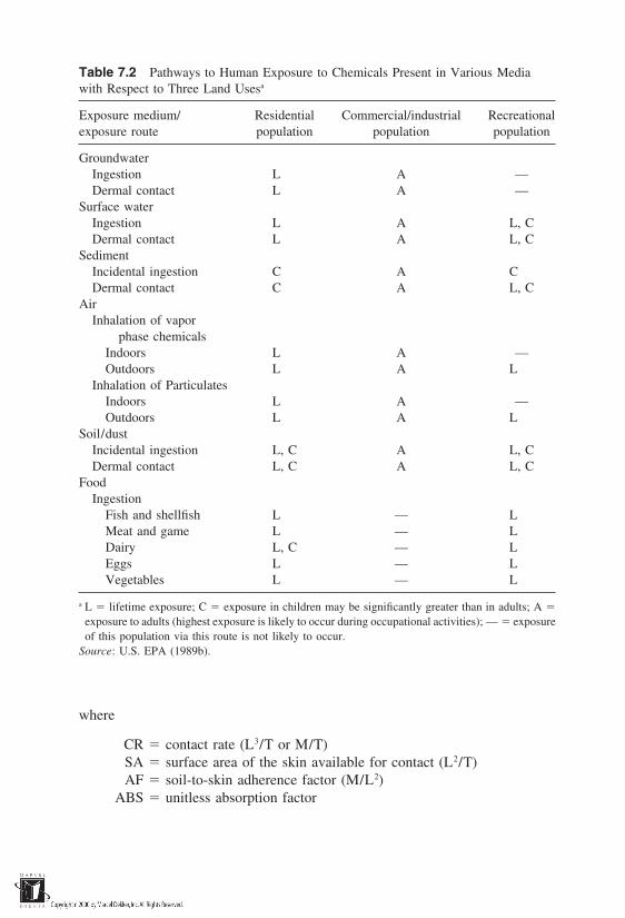
Table 7.2 Pathways to Human Exposure to Chemicals Present in Various Mediawith Respect to Three Land Usesa

Exposure medium/ Residential Commercial/industrial Recreationalexposure route population population population

GroundwaterIngestion L A —Dermal contact L A —

Surface waterIngestion L A L, CDermal contact L A L, C

SedimentIncidental ingestion C A CDermal contact C A L, C

AirInhalation of vapor

phase chemicalsIndoors L A —Outdoors L A L

Inhalation of ParticulatesIndoors L A —Outdoors L A L

Soil/dustIncidental ingestion L, C A L, CDermal contact L, C A L, C

FoodIngestion

Fish and shellfish L — LMeat and game L — LDairy L, C — LEggs L — LVegetables L — L

a L lifetime exposure; C exposure in children may be significantly greater than in adults; A

exposure to adults (highest exposure is likely to occur during occupational activities); — exposureof this population via this route is not likely to occur.

Source: U.S. EPA (1989b).

where

CR contact rate (L3/T or M/T)SA surface area of the skin available for contact (L2/T)AF soil-to-skin adherence factor (M/L2)

ABS unitless absorption factor

Table 7.3 Principal Processes of Contaminant Alteration and Transport to ExposurePoints and Human Intake Boundaries

Receivingmedium Release mechanism Release source

Air Volatilization Surface wastes—lagoons, ponds, pits,spills

Contaminated surface waterContaminated surface soilContaminated wetlandsLeaking drums

Fugitive dust generation Contaminated surface soilWaste piles

Surface water Surface runoff Contaminated surface soilEpisodic overland flow Lagoon overflow

Spills, leaking containersGroundwater seepage Contaminated groundwater

Groundwater Leaching Surface or buried wastesContaminated soil

Soil Leaching Surface or buried wastesSurface runoff Contaminated surface soilEpisodic overland flow Lagoon overflow

Spills, leaking containersFugitive dust generation/ Contaminated surface soil

deposition Waste pilesContaminated surface soil

TrackingSediment Surface runoff Surface wastes—lagoons, ponds, pits,

spillsEpisodic overland flow Contaminated surface soilGroundwater seepage Contaminated groundwaterLeaching Surface or buried wastes

Contaminated soilBiota Uptake Contaminated soil, surface water, sedi-

(direct contact, ingestion, ment, groundwater or airinhalation) Other biota

Source: U.S. EPA (1989b).

The numerical magnitudes of AF and SA are of the order of 1.45–2.77 mg/cm2

and 0.3 m2 per specified time, respectively. ABS varies widely for differentcontaminants.

It is often necessary to develop and use numerical indices for assessing thefactor of safety against damaging health effects of human exposure to contami-

nants. Thus, the risk of a damaging health effect (e.g., cancer) can be estimatedby combining contaminant exposure equations with potency estimates of the con-taminant with respect to the disease for which the estimate is made. Within regu-latory frameworks, it is convenient to consider carcinogenic risks and noncarcino-genic risks separately in the risk characterization phase.

7.2.1 Carcinogenic Risks

Some chemical contaminants are carcinogens (cancer causing). The approach toquantifying cancer risk is to estimate the incremental probability that an individ-ual will develop cancer over a lifetime due to exposure to the chemical. Twomethods are commonly used for this estimate: the linear low dose model for risksthat are below 0.01; and the one-hit model for exposure conditions in which theprobable dose is high (0.01). In the linear low-dose model, the carcinogenicrisk is computed as follows:

Rc Ic ⋅ SF (7.7)

where

Rc carcinogenic risk probability of an individual developingcancer due to exposure to the contaminant (unitless fraction)

Ic chronic intake averaged over 70 years (mg/kg-day)SF slope factor (mg/kg-day)1

The chronic daily intake is computed using the relevant form of the exposureequation (7.5). Conceptually, the slope factor is the ratio of cancer frequency tothe dose of the contaminant that is being evaluated. Generally it is the upper-bound (usually 95th percentile) confidence limit of the slope of the dose–responseplot expressed in units of (mg/kg-day)1. The magnitude of the slope factor canbe considered as the risk per unit dose of the contaminant. An intrinsic assumptionin the use of slope factors is that there is no threshold dose level below whichcancer risk is zero.

It may also be found convenient to express the carcinogenic effects of acontaminant in terms of the risk per unit concentration of the contaminant in themedium of human contact. This is particularly useful in assessments of the poten-tial health benefits of risk management technologies that may be effective incontaminant clean-up, containment, or other remedial actions. Unit risk can beestimated using Eq. (7.8):

UR SF ⋅ Ei

70 kg ⋅ 1000(7.8)

where

UR unit risk for the particular medium of interest (fraction per µg/m3)

Ei consumption rate for water (2 liters/day) or inhalation rate forair (20 m3/day)

The 70 kg used represents body weight and is included to cancel out the normal-ization for body weight in the definition of the slope factor. Also, the factor 1000is used as the denominator to convert from milligrams [unit of the slope factor:(mg/kg-day)1] to µg [unit of unit risk: (µg/m3)1 for air and (µg/L)1 for water].

Considering that cancer risk may be attributable to more than one contami-nant through a number of pathways or exposure routes, composite low-dose can-cer risk can be estimated using Eq. (7.9):

TRc k

j1

n

i1

(I ⋅ SF) ij (7.9)

where

TRc total cancer risk probability that an individual will developcancer (unitless fraction)

Iij chronic daily intake of the ith contaminant through the jthexposure pathway (mg/kg-day)

SF ij slope factor for the ith contaminant contacted through the jthexposure pathway [(mg/kg-day)1]

n total number of carcinogeneous contaminantsk total number of exposure pathways

For the one-hit model, the risk of an exposed individual developing cancerdue to a contaminant through a specific pathway can be computed using Eq.(7.10):

Rc 1 exp(Ic ⋅ SF) (7.10)

The parameters are as defined for Eq. (7.7). The corresponding relationship foran aggregate value of risk for all carcinogeneous contaminants for all exposureroutes is

TRc k

j1

n

i1

[1 exp(Ic ⋅ SF) ij] (7.11)

All parameters are as defined for Eq. (7.9). In using Eqs. (7.9) and (7.11), strictadditivity of cancer risks from identified carcinogens is assumed. Synergistic ef-fects are neglected. Furthermore, the effects are summed equally for the carcino-gens.

7.2.2 Noncarcinogenic Risks

In the case of noncarcinogens, the adverse effect of exposure to a contaminantis assumed not to be significant (or manifestive) unless the subject is exposed todoses above a critical level. The existence of the threshold dose is attributableto the body’s protective physiological mechanism. The challenge is to determinethe upper bound of the threshold dose for use as the body’s tolerance limit. Vari-abilities in human susceptibilities to the same dose of a contaminant and uncer-tainties associated with extrapolations of toxicological data from one populationto another necessitate continuous updating of data on critical doses.

Assessments of the risk of noncarcinogenic effects of contaminants areusually based on the reference dose, RfD, which is discussed in detail by theU.S. EPA (1986). As defined by the U.S. EPA (1989b), the chronic RfD is thedaily exposure level for the human population (including subpopulations) that islikely to be without an appreciable risk of deleterious effects during a lifetime.Values of chronic RfD are meant to be protective of the effects of long-termexposure to a contaminant, whereas subchronic RfD addresses the effects ofshorter-term exposures. RfD is currently used as a replacement for its precursors:the acceptable daily intake (ADI) and the acceptable intake for chronic exposure(AIC).

Considerable uncertainty (of the order of one magnitude or more) character-izes estimates of RfD. This parameter can be estimated from the results of dose–response experiments for noncarcinogens and/or through the use of relevant toxi-cological data. In dose–response experiments, it is useful to determine the re-sponse limits which can be used with appropriate uncertainty factors to estimateRfD as shown in Eq. (7.12):

RfD NOAEL

n

i1UF iMF

(7.12)

where

RfD reference dose (mg/kg⋅day)NOAEL no-observed-adverse-effect-level contaminant dose (mg/

kg ⋅ day)UFi uncertainty factorMF modifying factor ranging in magnitude from 1 to 10 to be

applied by the evaluator to account for uncertainties inthe database for the chemical when such uncertainties arenot covered by any of the UFs

NOAEL, which can be computed from the results of dose–response experiments,is the exposure level at which no biologically or statistically significant increasesin the severity or frequency of adverse effects occur in the exposed populationrelative to the control population. Other dose–response levels are, the no-observed-effect level (NOEL) and the lowest-observed-adverse-effect level(LOAEL). NOEL pertains to all effects (adverse or positive). Uncertainty factorsare generally applied to address the following sources of uncertainty:

1. Variability in the general population which renders subpopulationssuch as children and the elderly more sensitive to contaminants

2. Extrapolation of dose–response data from experiments on animals torisk characterization for humans (interspecies variability between hu-mans and other mammals)

3. Use of NOAEL derived from subchronic rather than from chronic data4. Use of LOAEL rather than NOAEL

Reference dose data are used to develop a noncancer quotient for a contaminantfor an exposure route as follows:

H Ic

RfD(7.13)

where

H noncancer hazard quotient (unitless)

Ic and RfD are as previously defined. Their units as well as the period of coverage(chronic or subchronic) must be kept identical. Considering that at most pollutedsites, several noncarcinogens within a medium may be taken in through one ormore exposure pathways, the aggregate risk can be expressed using Eq. (7.14):

TH k

j1

n

i1

Hij (7.14)

TH k

j1

n

i1 Iij

RfD ij (7.15)

where

TH total hazard index (unitless)Iij exposure level (intake) for the ith contaminant through the

jth exposure pathwayRfD ij reference dose for the ith contaminant for the jth pathway

(mg/kg⋅day)Hij hazard quotient for the ith contaminant and jth pathway

n total number of contaminants that exhibit noncarcinogeniceffects

k total number of exposure pathways

From the configuration of Eq. (7.15), values of H and TH that are much less than1.0 are more desirable than those that approach 1.0 or greater. Values greaterthan 1.0 can be used to justify risk management actions for the site concerned.

Within the context of geoenvironmental engineering, the purpose of expo-sure assessment, and the risk assessment which encompasses it, is to assess theneed for implementation of an engineering control measure. Essentially, suchmeasures may result in risk reduction through impact on the concentration ofcontaminants at the source and/or exposure points. The configuration of a con-taminated site, the characteristics of the transport medium for released contami-nants, climatic factors, and proximity of exposure points to human habitat aresome of the critical factors that affect (directly or indirectly) the magnitudes ofrisks for which equations have been discussed in this chapter. The focus of thisanalysis has been human health risk. Ecological risk can also be assessed, al-though many more factors need to be considered. Some investigators have devel-oped site vulnerability indices for use in scaling risks and hazards associated withcontaminated sites and sites that may be sensitive to contamination. Examplesof these indices are the DRASTIC Index (Aller et al., 1985), the Multi-attributeUtility Analysis Model (Call and Merkhofer, 1988), and a host of other modelsdescribed by Hushon and Kornreich (1984), Shahane and Inman (1987), Mayer-nik and Fehrenkamp (1992), Merz (1988), and Mikroudis et al. (1986).

7.3 RISK-BASED ESTIMATION OF REQUIREDCLEAN-UP LEVELS

The primary objective of polluted-site remediation programs such as clean-upand containment is to reduce the concentrations of targeted contaminants at thesource and/or exposure points such that risk can be reduced to an acceptablelevel. By specifying the maximum acceptable risk and rearranging risk estimationequations such as (7.5), (7.7), (7.9), (7.10), (7.11), (7.13), and (7.15), the maxi-mum concentration of specific pollutants that are allowable in each medium canbe back-calculated. This approach has utility with respect to the selection of reme-diation schemes (including technology) that could be effective in reducing con-taminant concentrations to desirable levels.

Usually, it is advisable to specify the land use (e.g., commercial, residential,or agricultural) before applying the equations. The land use time primarily affectsthe default values or direct estimates of the magnitudes of some of the parameters

of the risk equations used in back-calculations of the maximum concentrationsof target contaminants. As discussed in the preceding sections, carcinogenic ef-fects are treated separately from noncarcinogenic effects. Also, each contami-nated medium (water, soil, or air) can exhibit risks that are attributable to oneor more pathways. For example, for residential land use, risk from the watermedium can be represented as follows, for the purpose of setting up equationsfor the back-calculation of the maximum acceptable concentration limits for con-taminants:

Total risk from water risk of water ingestion

risk of inhalation of volatiles from water

For carcinogenic effects, the maximum acceptable risk is usually specifiedas 106, while a total hazard quotient of 1.0 is usually the upper limit for noncar-cinogenic effects. The approach is to calculate the maximum concentration of acontaminant at the exposure point through consideration of all the pathways thatcan contribute to risk attributable to the contaminant.

7.3.1 Clean-up Level for Soil

For both residential and commercial/industrial land uses, the ingestion exposurepathway applies. Additionally, for the commercial/industrial pathway, other path-ways are inhalation of volatiles from soil and inhalation of particulates from soil(by workers).

Residential

For residential land use, the total risk is attributable to the ingestion pathway.For carcinogenic effects, the relevant risk equation and its rearrangement to soilfor maximum concentration are presented as Eqs. (7.16) and (7.17).

Rc SF ⋅ Ic SFo (C 106 kg/mg)(EF)(IF)(AT 365 days/year) (7.16)

C (Rc)(AT 365 days/year)

(SF 106 kg/mg)(EF)(IF)(7.17)

where

C risk-based remediation level for the target contaminant (mg/kgof the contaminant in soil)

Rc target excess individual cancer risk (usually specified as 106)SFo oral cancer slope factor [(mg/kg⋅day)1]AT averaging time (years); a default value of 70 years

EF exposure frequency (days/year); a default value of 350 days/year

IF age-adjusted ingestion factor (mg ⋅ yr/kg ⋅ day); default valueof 114 mg ⋅ yr/kg ⋅ day [Note that ED of Eq. (7.5) isincorporated herein]

For noncarcinogenic effects, the noncancer hazard quotient presented as Eq.(7.13) can be rearranged as follows:

H 1

RfDo

[Ic] 1

RfDoC 106 kg/mg)(EF)(IF)

(AT 365 days/year) (7.18)

C (RfDo)(H )(AT 365 days/year)

(106 kg/mg)(EF)(IF)(7.19)

where

H target hazard index (unitless); usually specified as 1.0RfDo oral chronic reference dose (mg/kg ⋅ day)

AT Averaging time (years); default value 30 years

Other parameters and their corresponding default values are as stated forEqs. (7.16) and (7.17).

Commercial/Industrial

For commercial or industrial use, the disturbance of soils by heavy equipmentand traffic is assumed to increase the potential for emission of particulates andvolatiles which could be inhaled by workers. Additional exposure pathways ex-emplified by dermal exposure may also be relevant at some sites. It is alwaysnecessary to identify the relevant exposure pathways for the particular site.

The concentration limit for a contaminant in soil at a site that is to be usedfor commercial/industrial purposes, based on health effects, can be computedfrom the following setup of the risk equation (only three pathways are used inthe following example).

Risk risk form intake due to soil ingestion by workersrisk from intake due to inhalation of volatiles by workersrisk from intake due to inhalation of particulates by workers

For carcinogenic effects, the two inhalation risks (for volatiles and particu-lates) can be combined such that the resulting total risk equation assumes theform of Eq. (7.20), which is the expanded form of Eq. (7.9).

(7.20)TRc

(SFo)(C 106 kg/mg)(EF)(ED)(IRs)(BW)(AT 365 days/year)

(SFi)(C)(EF)(ED)(IRs)(1/VF) (1/PEF)(BW)(AT 365 days/year)

By rearrangement to produce an expression for the concentration C,

C (TRc)(BW)(AT 365 days/year)

(EF)(ED) [(SFo 106 kg/mg)(IRs) (SFi)(IRa)(1/VF) (1/PEF)](7.21)

where

C chemical concentration in soil (mg/kg)TRc target excess individual lifetime cancer risk (unitless; usually

specified as 106)SFi inhalation cancer slope factor for the contaminant [(mg/kg ⋅

day)1]SFo oral cancer slope factor for the contaminant [(mg/kg ⋅ day)1]BW adult body weight (kg); default value 70 kgAT averaging time (year); default value 70 yearsEF exposure frequency (days/year); default value 250 days/

yearED exposure duration (years); default value 25 yearsIRs soil ingestion rate (mg/day); default value 50 mg/dayIRa workday inhalation rate (m3/day); default value 20 m3/dayVF soil-to-air volatilization factor for the chemical (m3/kg)

PEF particulate emission factor (m3/kg); default value 4.63 109 m3/kg

The emission factors, VF and PEF, can be estimated as follows:

VF (LS)(V )(DH)A [(3.14)α (T)]0.5

(2)(Dei)(E)(Kas)(103 kg/g) (7.22)

where

α (Dei)(E)E (ρs)[(1 E)/Kas]

VF soil to air volatilization factor (m3/kg)

LS length of the contaminated area (m)V wind speed in the mixing zone (m/s); default value 2.25

m/sDH diffusion height (m); default value 2 m

A area of contamination (cm2)Dei effective diffusivity of the contaminant; default estimate

Di E0.33

E true soil porosity (unitless); default value 0.35Kas soil–air partition coefficient (g soil/cm3 air); default value

41(H/Kd)ρs true soil density (particle density) (g/cm3); default value

2.65 g/cm3

T exposure interval(s); default value 7.9 108 sDi molecular diffusivity of the contaminant (cm2/s)H Henry’s law constant of the contaminant (atm ⋅ m3/mol)

Kd soil–water partition coefficient of the contaminant (cm3/g) (Koc)(OC) for organic contaminants

Koc organic carbon partition coefficient of the contaminant (cm3/g)OC organic carbon content of the soil (fraction); default value

0.02

It should be noted that α does not represent any specific fundamental factor butis merely a collection of terms and has units of cm2/s. The U.S. EPA (1991) alsoprovides Eq. (7.23) for estimation of the particulate emission factor, PEF:

PEF (LS)(V )(DH)(3600 s/h)A 1000 g/kg

(0.036)(1 G)(µm/µ t)[F(X)] (7.23)

where

PEF particulate emission factor (m3/kg); default value 4.63 109 m3/kg

G fraction of vegetative cover (unitless); default value 0µm mean annual wind speed (m/s); default value 4.5 m/sµ t equivalent threshold value of wind speed at 10 m height

(m/s); default value 12.8 m/sF(X ) A function of the ratio µm/µ t, unitless); default value

0.0497

All other parameters are as defined for Eq. (7.22). The number 0.036 in Eq. (7.23)is the approximate magnitude of the respirable fraction of particulates in unitsof g/m2-hr.

For noncarcinogenic effects relevant to the soil medium in commercial/

industrial land use, the setup of the risk equation for back-calculation of the targetcontaminant concentration is similar to the approach represented by Eq. (7.20).A total target hazard index value of 1.0 and relevant values of reference doseare used.

7.3.2 Clean-up Level for Groundwater

Following an approach similar to that used for soils in Section 7.3.1, the riskequation can be set up to cover as many exposure pathways as are found to besignificant for a site. For residential land use, ingestion of water and inhalationof volatiles from household water are two common pathways. It may be necessaryto reduce the exposure frequency, EF, for commercial land use calculations. Us-ing the example of carcinogenic effects for a groundwater contaminant within aresidential environment, the risk-based maximum concentration limit for a com-bination of ingestion and volatiles inhalation pathways is as follows:

TRc (SFo)(C )(IRw)(EF)(ED)(BW)(AT)(365 days/year) (SFi)(C )(K)(IRa)(EF)(ED)

(BW)(AT)(365 days/year) (7.24)

By rearrangement,

C (TRc)(BW)(AT 365 days/year)

(EF)(ED)[(SFi)(K )(IRa) (SFo)(IRw)](7.25)

where

C risk-based chemical concentration in water (mg/liter)TRc target individual lifetime cancer risk (unitless), usually

specified as 106

SFi inhalation cancer slope factor for the contaminant [(mg/kg ⋅day)1]

SFo oral cancer slope factor for the contaminant [(mg/kg⋅day)1]BW adult body weight (kg); default value 70 kgAT averaging time (years); default value 70 yearsEF exposure frequency (days/years); default value 350 days/

yearED exposure duration (years); default value 30 yearsIRa daily indoor inhalation rate (m3/day); default value 15 m3/

dayIRw daily water ingestion rate (liters/day); default value 2

liters/dayK volatilization factor (unitless); default value 0.0005

1000 liters/m3 as suggested by U.S. EPA (1991)

Essentially, the calculation of risk-based concentration levels for remedialaction requires various categories of data: toxicological data, data on the charac-teristics of the contaminant and exposure media, land use data, as well as thecultural activities of the target population. Several uncertainties are associatedwith the data used in such calculations. Nevertheless, the risk-based approachprovides the most rational way of justifying clean-up actions and evaluating tech-nologies of knownoperational efficiencies with respect to the extent to whichtheir application can reduce human health risk at an exposure point.

REFERENCES

Aller, L. Bennett, T., Lehr, J. H., and Petty, R. J. (1985). DRASTIC: A standardizationsystem for evaluating groundwater pollution potential using hydrogeologic settings.Technical Report Under Cooperative Agreement CX-819715-01, Office of Re-search and Development, U.S. Environmental Protection Agency, Ada, OK.

Call, Hollis J., and Merkhofer, Miley W. (1988). A Multi-attribute Utility Analysis Modelfor Ranking Superfund Sites. Proc. 9th Natl. Superfund Conf., Washington, DC,pp. 44–54.

Hushon, J. M., and Kornreich, M. R. (1984). Scoring systems for hazard assessment. In:J. Sacena (ed.), Hazard Assessment of Chemicals, Vol. 3., pp. 63–109, AcademicPress, Orlando, FL.

Lee, C. H., Wang, H. C., Lin, C. M., and Yang, C. C. (1994). A long-term leachabilitystudy of solidified wastes by the multiple toxicity characteristic leaching procedure.J. Hazardous Materials, 38:65–74.

Lerose, G. A. (1995). When to use the TCLP test method and when not to. Virginia’sEnvironment, July.

Manahan, S. E. (1990). Hazardous Waste Chemistry, Toxicology and Treatment. LewisPublishers, Chelsea, MI.

Mayernik, J. A., and Fehrenkamp, K. (1992). A new model for conducting quantitativeecological risk assessments at hazardous waste sites. Proc. 13th Annual Natl. HMC/Superfund Conf. and Exhibition, Washington, DC, pp. 813–819.

Merz, E. R. (1988). Criteria for long-term hazard assessment of chemotoxic and radiotoxicwaste disposal. Proc. Int. Topical Meeting on Nuclear and Hazardous Waste Man-agement, Pasco, WA, pp. 316–318.

Mikroudis, G. K., Fang, H-Y, and Wilson, J. L. (1986). Development of Geotox expertsystem for assessment of hazardous waste sites. Proc. Int. Symp. on EnvironmentalGeotechnology, Bethlehem, PA, Vol. 1, pp. 223–232.

National Research Council. (1988). Complex mixtures. A report of the Committee onMethods for the in Vivo Toxicity Testing of Complex Mixtures, Board on Environ-mental Studies and Toxicology, National Research Council, Washington, DC.

Shahane, A. N., and Inman, R. C. (1987). Review of available pesticide assessment ratingsystems. In: J. Saxena (ed.), Hazard Assessment of Chemicals, pp. 103–300, Hemi-sphere, Washington, DC.

Stults, R. G. (1993). Hazardous waste: Identification. Hazmat World, March: 55–60.U. S. EPA. (1986). Guidelines for the health assessment of suspect developmental toxi-

cants. 51 profiles. U.S. Environmental Protection Agency, in 52 Federal Register,34028, September 24.

U. S. EPA. (1989a). Stabilization/solidification of CERCLA and RCRA wastes: Physicaltests, chemical testing procedures, technology screening, and field activities, EPA/625/6-89/022. Office of Research and Development, U. S. Environmental Protec-tion Agency, Washington, DC.

U. S. EPA. (1989b). Risk assessment guidance for Superfund: Volume 1, human healthevaluation manual, part A, EPA/540/1-89/002. Office of Emergency and RemedialResponse, U. S. Environmental Protection Agency, Washington, DC.

U. S. EPA. (1991). Risk assessment guidance for Superfund: Volume 1, human healthevaluation manual, part B, development of risk-based preliminary remediationgoals, EPA/540/R-23/003. Office of Research and Development, U. S. Environ-mental Protection Agency, Washington, DC.

Whittemore, A. and Keller, J. B. (1978). Quantitative theories of carcinogens SIAM Rev.,20:1–30.

8Principles of Site and GeomaterialTreatment Techniques

The focus of this chapter is on the principles that underlie various treatment tech-niques for contaminated sites and excavated geomaterials. Several vendors havegiven a plethora of trade names to derivatives and combinations of technologiesthat are based on the basic treatment approaches and techniques described herein.This chapter focuses not on the technologies but on the general principles. Wherenecessary and possible, equations which describe the quantitative relationshipsamong the parameters that define the effectiveness of techniques are provided.

8.1 TREATMENT APPROACHES

In Chapter 7, the characteristics which determine the categorization of wastes as‘‘hazardous,’’ were discussed. Furthermore, quantitative expressions for expo-sure assessment were found in that chapter to contain contaminant concentra-tion. For off-site areas, exposure magnitudes are also influenced by the capacityof a contaminant to travel (mobility) from its source, through bounding media,to locations of concern. Treatment systems generally target the parameters thatdefine risk (human and/or ecosystem risks). The major categories of treatmentapproaches aimed at reducing risks and exposure levels of contaminants are:

Modification of the chemical structure of the contaminant to reduce itstoxicity

Modification of the chemical form of the contaminant to reduce its mobility(gas form is more mobile than liquid form, and liquid form is more mo-bile than solid form)

Change of contaminant phase to reduce volumeModification of the characteristics of the transport media of the contaminantRemoval of the contaminant from the site

With respect to the direct treatment of waste to change the negative charac-teristics that render the waste ‘‘hazardous,’’ the following basic treatment actionsare employed.

Corrosive waste pH adjustmentIgnitive waste Oxidation or reductionReactive waste Oxidation or reductionToxic waste pH adjustment for metals, and oxidation,

reduction, and pretreatment for organics

Usually, a ‘‘treatment train’’ is designed to treat contaminated media where thechemistry is complex and existing technologies are effective for only some con-taminants in specific concentration ranges.

8.2 IN-SITU VERSUS EX-SITU TREATMENT

To the extent possible, in-situ treatment is preferable to ex-situ treatment becausethe former does not involve the expensive excavation and handling of materials.However, in-situ treatment is sometimes not possible because the treatment tech-nique selected requires greater control of the processes than can be done in thesubsurface.

Batch treatment systems are commonly used in ex-situ treatment. The con-taminated media have the maximum possibility of contact with the energy ormaterial used in treatment. Under in-situ conditions, that potential decreases im-mensely and is determined by several geotechnical/soil hydrological factors suchas soil permeability, stratification, flow channeling, and intensity of the energyor treatment fluid pressure imposed on the soil. Table 8.1 shows ratings developedby a U.S. National Research Council Panel (Macdonald and Kavanaugh, 1994)for the cleanup of groundwater contaminated by various substances in a varietyof hydrogeologic settings.

8.3 BASIS FOR TREATMENT TECHNOLOGY SELECTION

For any contaminated site or material, there is usually a number of treatmenttechnologies that could be selected. The selection criteria for such technologiesare summarized below, using information published by Ram et al. (1993) andLaGrega and Evans (1987).

Table 8.1 Ratings of the Relative Ease of Cleaning up Contaminated Groundwater

Contaminant chemistry

StronglyMobile, sorbed,

dissolved dissolved Strongly Separate Separate(degrades/ Mobile, (degrades/ sorbed, phase phase

Hydrogeology volatilizes) dissolved volatilizes) dissolved LNAPLa DNAPLb

Homogeneous, 1 1–2 2 2–3 2–3 3single layer

Homogeneous, 1 1–2 2 2–3 2–3 3multiplelayers

Heterogeneous, 2 2 3 3 3 4single layer

Heterogeneous, 2 2 3 3 3 4multiplelayers

Fractured 3 3 3 3 4 4

The difficulty of cleanup is influenced by the hydrogeologic conditions and contaminant chemistryat a site. The NRC report classified the relative ease of cleanup as a function of these two conditionson a scale of 1–4, where 1 is the easiest and 4 the most difficult. The 1–4 scale used in this tableshould not be viewed as objective and fixed, but as a subjective, flexible method for evaluating sites.Other factors that influence ease of cleanup, such as the total contaminant mass at a site and thelength of time since it was released, are not shown in this table.a Light non-aqueous-phase liquid.b Dense non-aqueous-phase liquid.Source: Macdonald and Kavanaugh (1994).

1. Applicability of the technology to the chemistry and concentrations ofcontaminants at the site. This is the principal criterion for the selection of treat-ment technologies. Treatment system effectiveness may vary with changes inreaction conditions, contaminant concentrations, and contaminant compositions.Preliminary information about the contaminants present at a site may give anindication about the treatment technique that is likely to work. For example, con-taminants with Henry’s law constant greater than 0.1 are removable by air strip-ping technique (Ram et al., 1993).

2. Possibility of effectiveness enhancement with other treatment technolo-gies. Some technologies may be selected because they can be combined withothers in a ‘‘treatment train’’ that is more effective than each of the constituenttechnologies alone. Each technology may be effective only for a particular con-

taminant, in a specific concentration range, under a given set of environmentalconditions. Outside these bounds, the ancillary technology in the treatment trainwould be designed to clean up the contaminant(s). Examples of treatment trainsused in the Superfund Remedial Actions of the U.S. Environmental ProtectionAgency during the period 1982–1995 are illustrated in Figure 8.1.

3. Site Characteristics. Site characteristics play a very significant role

Figure 8.1 Treatment trains used in various superfund projects of the U.S. Environmen-tal Protection Agency for the period 1982–1995 (U.S. EPA 1996).

in determining the potential effectiveness of a technology. For example, sometreatment technologies such as soil venting and air sparging require that the soilformation be reasonably permeable to air for the removal of contaminants. Also,in clays that have negligible permeability, it may be difficult to deliver nutrientsto microbes if in-situ bioremediation is selected as the treatment technology.

4. Required treatment time. Due to differences in the kinetics of the pro-cesses involved, different treatment technologies require different durations forcompletion. However, it should be noted that chemical and/or physical reactiontime is only a fraction of the time required to implement a treatment technology.Time is also required for site preparation, equipment setup, and site safety pro-grams. Time may be a limitation for some technologies if risk assessments andother regulatory considerations specify a time limit for the completion of cleanup.

5. Regulatory acceptance of the technology. Some technologies may befavored by regulations such that the decision maker has a limited number oftreatment options from which to select. For example, if regulations specify thatoff-gas from a treatment technique must be treated, a technology such as airstripping that produces off-gas may fall out of contention because of the addi-tional cost of off-gas treatment.

6. Cost-effectiveness of the treatment technology. In most cases, this isthe overriding criterion. Most technologies could be effective if resources areunlimited for their implementation. Cost-effectiveness is a good measure of thereturns on investment of resources on a technology at a contaminated site. It alsorelates to the duration of implementation, which affects cost.

Using various criteria, most of which are subcategories of the primary crite-ria described above, the U.S. EPA (1993) developed the screening table shownas Table 8.2 for selecting treatment technologies for various classes of contami-nants. In order to address uncertainties about the potential effectiveness of spe-cific technologies in treating contaminated media present at a site, treatment feasi-bility studies are usually conducted in two stages before full implementation inthe field. The first stage is bench-scale feasibility studies, in which treatmentprocess parameters are analyzed through testing of samples of the contaminatedmedia in the laboratory. Based on the results obtained, a pilot-scale feasibilitystudy is conducted to demonstrate the effectiveness of the technology in the fieldbefore its full-scale operation.

8.4 PUMP-AND-TREAT PRINCIPLES

Pump-and-treat systems involve the removal of contaminated groundwaterthrough the use of extraction wells. The extracted groundwater is then treatedabove ground. There are two principal categories of pump-and-treat systems:

Table 8.2 Remediation Technologies Screening Table

a The listing of contaminant groups is intended as a general reference only. A technology may treat only selected compounds within the contaminant groups listed.Further investigation is necessary to determine applicability to specific contaminants.

b The definition of this factor is not applicable to these technologies. They are, by design, the final step in treatment processes.* Conventional technologies/processes. Contaminant Codes: 1–Halogenated volatile organics; 2 -Halogenated semivolatile organics; 3–Non-halogenated volatile

organics; 4–Non-halogenated semivolatile organics; 5–Fuel hydrocarbons; 6–Pesticides; 7–Inorganics.Target contaminants are listed first and in bold type. RatingCodes: , better; , average; , worse; I, inadequate information; NA, not applicable.

Source: U.S. EPA (1993).

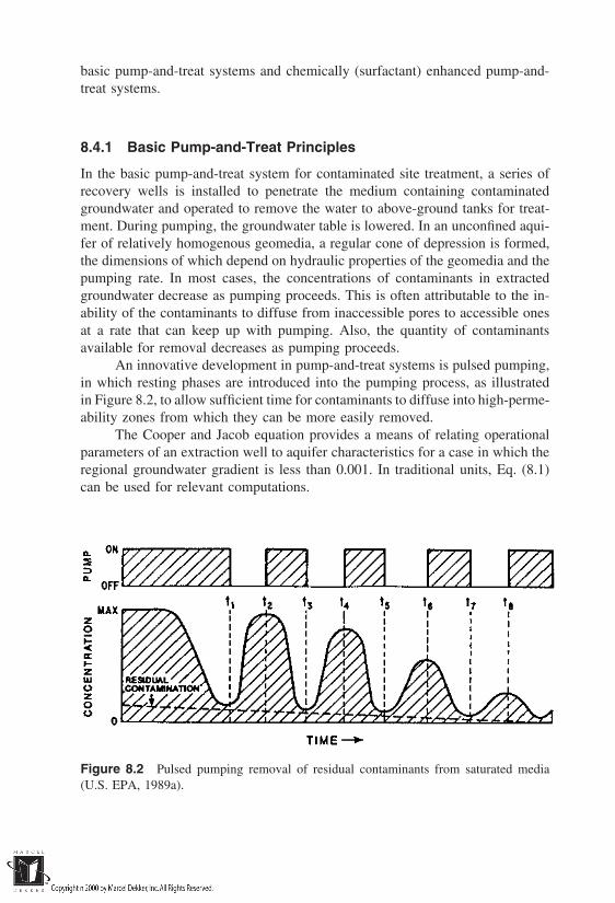
basic pump-and-treat systems and chemically (surfactant) enhanced pump-and-treat systems.

8.4.1 Basic Pump-and-Treat Principles

In the basic pump-and-treat system for contaminated site treatment, a series ofrecovery wells is installed to penetrate the medium containing contaminatedgroundwater and operated to remove the water to above-ground tanks for treat-ment. During pumping, the groundwater table is lowered. In an unconfined aqui-fer of relatively homogenous geomedia, a regular cone of depression is formed,the dimensions of which depend on hydraulic properties of the geomedia and thepumping rate. In most cases, the concentrations of contaminants in extractedgroundwater decrease as pumping proceeds. This is often attributable to the in-ability of the contaminants to diffuse from inaccessible pores to accessible onesat a rate that can keep up with pumping. Also, the quantity of contaminantsavailable for removal decreases as pumping proceeds.

An innovative development in pump-and-treat systems is pulsed pumping,in which resting phases are introduced into the pumping process, as illustratedin Figure 8.2, to allow sufficient time for contaminants to diffuse into high-perme-ability zones from which they can be more easily removed.

The Cooper and Jacob equation provides a means of relating operationalparameters of an extraction well to aquifer characteristics for a case in which theregional groundwater gradient is less than 0.001. In traditional units, Eq. (8.1)can be used for relevant computations.

Figure 8.2 Pulsed pumping removal of residual contaminants from saturated media(U.S. EPA, 1989a).

Q sT

264 1log(0.3Tt/r2

wS) (8.1)

where

Q pumping rate of a well (gal/min)s draw-down in the pumping well (ft)T aquifer transmissivity (gal/day per ft2)t duration of pumping (days)

rw radius of well (ft)S aquifer storativity (percentage of connected pore volumes in the

aquifer)

The desired draw-down and other parameters such as duration of pumping canbe specified and pumping rate optimized to achieve the desired removal.

The effectiveness of pump-and-treat techniques depends on several physi-cochemical factors besides the adequacy of the design and efficiency of the pump-ing installation.

The presence of NAPLs. NAPLs are non-aqueous-phase liquids and arediscussed in greater detail in chapter 5. They can be trapped in the poresof subsurface media by interfacial tension as illustrated in the top portionof Figure 8.3 such that they continue to be a source of contaminants withthe advance of pumping. Examples of NAPLs are halogenated aliphatichydrocarbons, halogenated benzenes, phthalate esters, and polychlori-nated biphenyls. The transfer of the NAPLs to the surrounding aqueousphase is by diffusive liquid–liquid partitioning. At high groundwater ve-locities, the contaminant is not allowed to build up significantly in theaqueous phase before advection, as illustrated in Figure 8.3. At lowgroundwater velocities, the extent to which NAPLs transfer occurs iscontrolled by its solubility.

Sorption effects. As contaminants travel with water under imposed hydrau-lic gradients, a fraction of the contaminants is removed through sorptionto subsurface media. As illustrated in Figure 8.4, initial desorption ofcontaminants from contaminated media may be relatively rapid. It willslow down as more tightly bound layers of the contaminant are reached.

Transport media hydraulic conductivity effects. High hydraulic conductivi-ties in the regime of 105 cm/s, favor pump-and-treat operations. Hetero-geneous media such as stratified layers of sand and clay may cause inter-layer exchange of contaminants in directions that are not necessarilytoward the extraction wells. Heterogeneity, even at a much smaller scalethan thick stratified layers of fine–and coarse-grained media, is a largecontributor to the ‘‘tailing effect,’’ in which contaminant concentration

Figure 8.3 Schematic illustration of solubility and diffusion limitations to pump-and-treat systems (Keeley, 1989).

in the extracted moisture persists at low levels even after prolongedpumping.

The following mathematical expression can be used to estimate contami-nant removal for a given rate and duration of pumping in a contaminated geologicmedium. It should be noted that this expression is essentially a delay functionof contaminant removal per unit of time and the goodness of fit of field data withthis simple model can be affected negatively by transport media stratification andother heterogeneities.

R C0 Ct

C0 1 exp Q

KdVt (8.2)

where

R contaminant removal rate (M/T)C0 initial concentration of contaminant (M/L3)Ct concentration of contaminant at time t (M/L3)V volume of contaminated groundwater (L3)

Figure 8.4 Schematic illustration of sorption limitations to pump-and-treat systems(Keeley, 1989).

Q pumping rate of the groundwater extraction system (L3/T)Kd distribution coefficient of the contaminant (M/L3)

Kd can be obtained, typically through contaminant sorption measurements in thelaboratory, for both organic and inorganic chemical compounds. For organiccompounds, it can be estimated using Eq. (8.3):

Kd Kocfoc (8.3)

where

Koc partition coefficient of the organic compound (M/L3)foc organic carbon fraction in the soil containing the contaminated

groundwater (unitless fraction)

The organic compound partition coefficient, Koc, can be estimated by correlationwith other parameters such as the octanol–water partition coefficient and solubil-

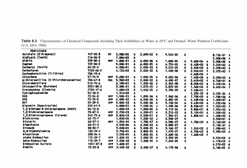
Table 8.3 Characteristics of Chemical Compounds Including Their Solubilities in Water at 20°C and Octanol–Water Partition Coefficients(U.S. EPA 1990)

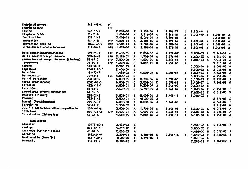
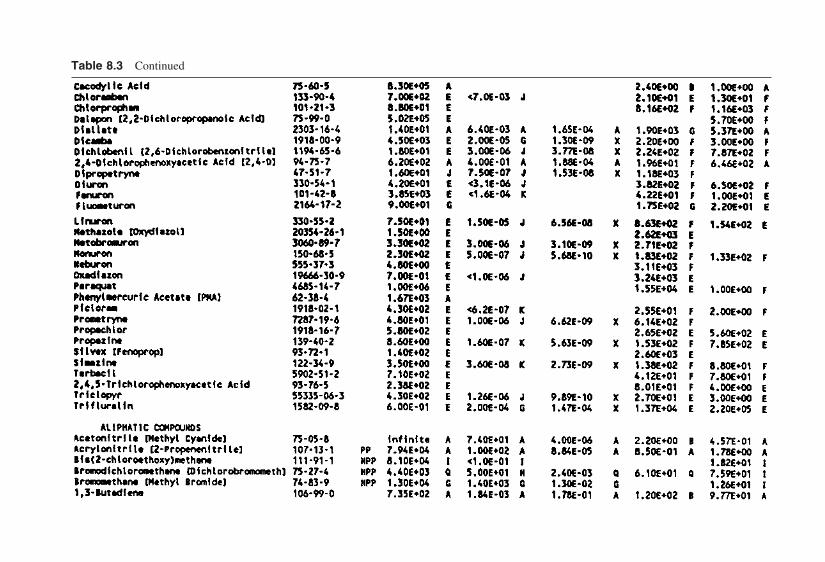
Table 8.3 Continued

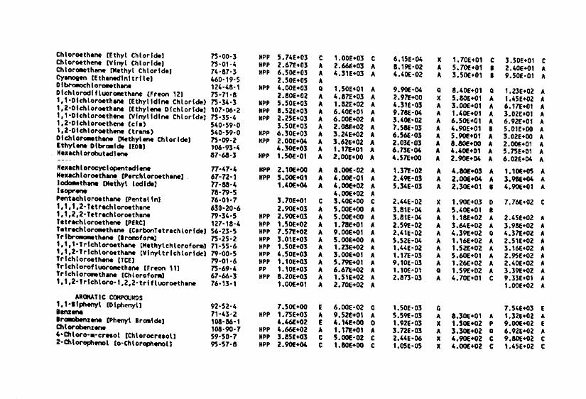
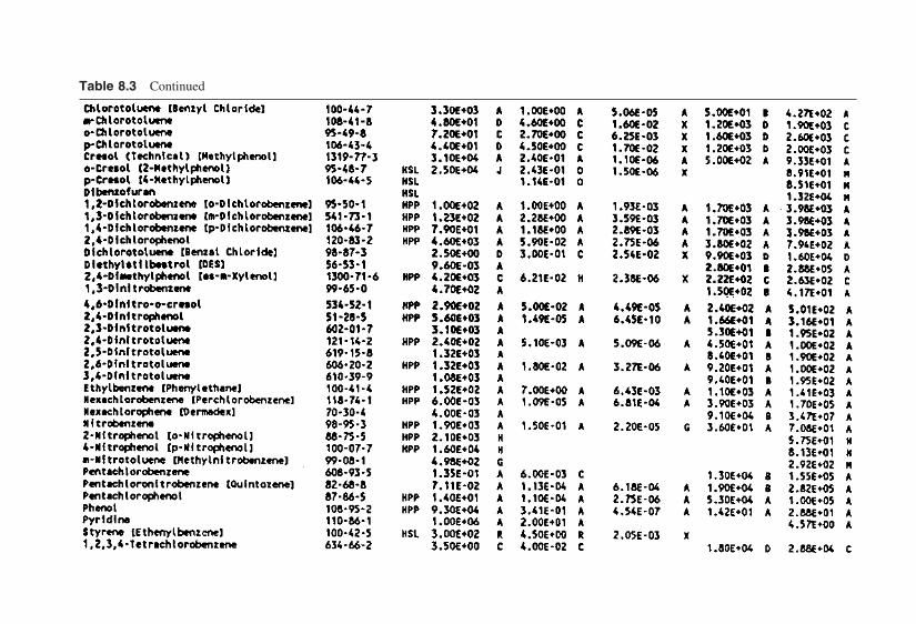
Table 8.3 Continued

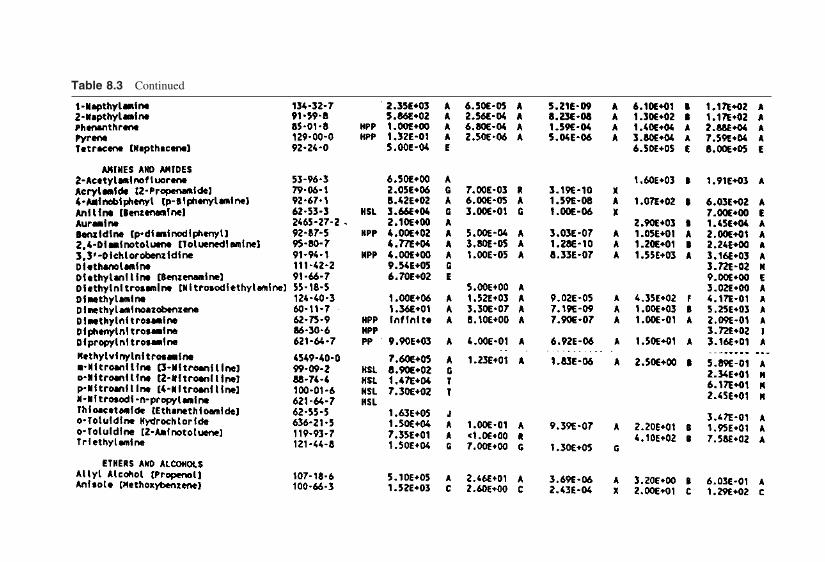
Table 8.3 Continued

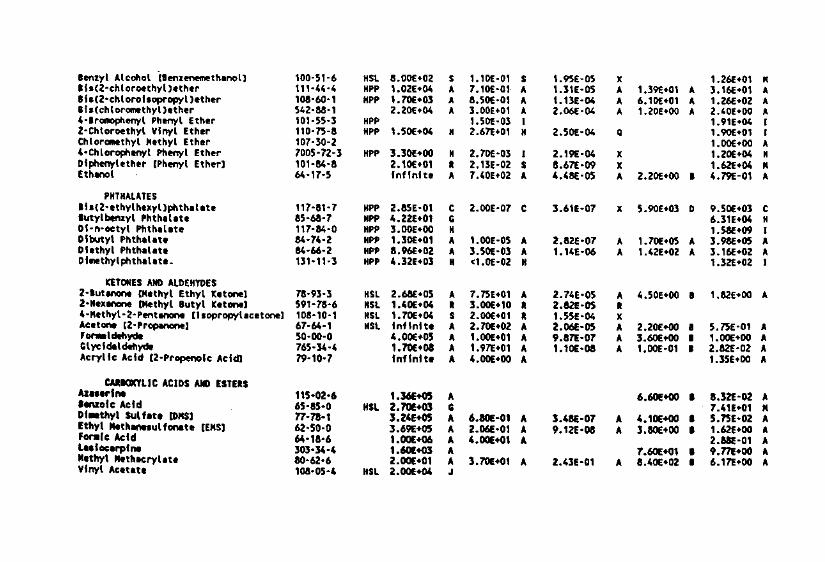
Table 8.3 Continued

Notes: PP Priority Pollutant; HSL Hazardous Substance List Parameter; HPP PP and HSL Parameters.A CONCAWE, 4/79, Protection of Groundwater from Oil Pollution.B Payne, J.R., and C.R. Phillips, 1985, Petroleum Spills in the Marine Environment, Lewis Publishers, Chelsea, MI.C National Institute for Petroleum and Energy Research, 1988, Personal communication.D Breuel, A., 1981, Oil Spill Cleanup and Protection Techniques for Shorelines and Marshlands, Noyes Data, N.J.E Cole-Parmer Co., 1989–1990, Equipment Catalog.F ASTM, 1985, Annual Book of ASTM Standards, Section 5, Petroleum Products, Lubricants, and Fossil Fuels, Philadelphia.G Chevron USA, Inc., 1988, Product Salesfax Digest, San Francisco.H Weast, R.C., (ed.), 1980–1981, CRC Handbook of Chemistry and Physics, 61st Edition, Cleveland.I Values calculated using ASTM viscosity-temperature charts for liquid petroleum products (ASTM D 341–77).J U.S. Coast Guard, 1979, CHRIS Hazardous Chemical Data.

Chevron USA, Inc., 1989, Personal Communication.Hunt, J.R., N. Sitar, and K.S. Udell, 1988, Monaqueous Phase Liquid Transport and Cleanup 1. Analysis of Mechanisms, in Water Resources Research, Vol.

No. 8, pp. 1247–1258. Values calculated based on: Absolute Viscosity (centipoise) Kinematic Viscosity (centistokes) Specific Gravity.

ity of organic compounds. The most common correlation equations (Yang andParker, 1998) are as follows:For nonpolar organic compounds:

log Koc 0.621 log S 3.95 (8.4)

log Koc 0.72 log Kow 0.49 (8.5)

For hydrophobic organic compounds:

log Koc log Kow 0.21 (8.6)

where

S aqueous solubility of the organic contaminant (mg/L)Kow octanol–water partition coefficient of the organic compound

(unitless)

Values of S and Kow for various chemical compounds are presented in Table 8.3as compiled by the U.S. EPA (1990) from a variety of references. Typical rangesof foc values are 0.0002–0.01 for sand and 0.01–0.08 for topsoil (which generallycontains clay) (Knox et al., 1993).

8.4.2 Chemical Enhancements Including Surfactants

Traditional pump-and-treat systems often lose effectiveness as the contaminantis removed until it reaches its residual saturation in the contaminated media.Residual saturation is the fluid saturation of the porous medium below whichfluid drainage will not occur. As illustrated in Figure 8.5, the capillary attractionof the residual liquid becomes excessively high at residual saturation, relative tothe imposed drainage forces. As discussed in Chapter 5, magnitude of residual

Figure 8.5 Trapped oily contaminant at residual saturation; flushing will not removeall of the trapped product because of capillary action (API, 1980).

saturation depends on the pore size distribution of the medium and physicochemi-cal properties of the porous medium and liquid. Estimates are often imprecisebecause of the numerosity of determining factors. For the case of oil ganglia inwater-filled soils, Hunt et al. (1988) used simple static force balance relations todevelop equations for two parameters, bond number Nb and capillary numberNc, which define conditions for ganglia mobilization to occur in the vertical andhorizontal directions, respectively:

Nb (ρcw ρw)gLvDp

σcw

4 (8.7)

Nb (µwvwLhDp)

Kσcw

4 (8.8)

where

Nb bond numberNc capillary number

ρcw contaminant (ganglia) water density (M/L3)ρw density of water (M/L3)g gravitation acceleration (L/S2)

Lv length of ganglia mobilized in the vertical direction (L)Lh length of ganglia mobilized in the horizontal direction (L)Dp mean pore throat diameter of the porous medium (L)σcw contaminant–water interfacial tension (M g/T)µw dynamic viscosity of water (M/LT)vw kinematic viscosity of water (L2/T)K permeability of the porous medium (L2/T)

Nonsatisfaction of Eqs. (8.7) and (8.8) implies that Lv and Lh are less than thelengths required for movement of ganglia to occur. Pressures or other parametersin the equations will need to change favorably before contaminant recovery canbe increased.

For contaminants that are sorbed much more strongly at residual concentra-tions by physicochemical interactions with the geologic media than at higherconcentrations, changes in the intensity of processes that control their distributioncoefficients define how much of the contaminant can be made available for re-moval within the tailing phase of pump-and-treat systems and/or other systemsthat involve contaminant extraction.

Use of reactive agents, including surfactants, is intended to promote con-taminant removal even at their residual saturations through one or a combinationof the following phenomena.

Figure 8.6 Illustration of the configuration of a type of surfactant, alkylbenzene sulfo-nate (U.S. EPA, 1992a).

Surfactant Action

Surfactants (SURface-ACTive-ageNTs) are generally large amphiphilic mole-cules with a hydrophobic chain moiety (made up of hydrocarbon or fluorocarbon)and a hydrophilic head (made up of polar or ionic groups) as illustrated in Figure8.6. Surfactants are amphiphilic in the sense that they can exist in one or moreforms: as a dissolved phase in water; as part of a micelle with other molecules;and as an adsorbed phase between a solid and its surrounding liquid. The interac-tion of surfactants with contaminated media can reduce the contaminant–waterinterfacial tension, σcw, and enable the contaminant to be more available andmobile. With an appropriate type and concentration of surfactant, data in litera-ture show that oil–water interfacial tension can be reduced from about 20 dynes/cm to about 104 dynes/cm.

Lowering of interfacial tension and dissolution of organic contaminants arelargest when the surfactant attains its critical micelle concentration (CMC). Amicelle, which is illustrated in Figure 8.7, is an aggregate formed (typically con-sidered to be spherical in shape) by surfactant molecules such that nonpolar tails

Figure 8.7 Aggregation of surfactant molecules into a micelle (U.S. EPA, 1992a).

occupy the interior of a sphere. Through a mechanism described as solubilization,nonpolar contaminants can dissolve in the micellar solution, thereby increasingthe overall solubility of the contaminant. Although its use in predictions of solu-bility for surfactant–organic compound combinations are often imprecise, solu-bility increases of three orders of magnitude following the addition of as littleas 5% by volume of an appropriate surfactant are possible.

There are more than 12,000 types of surfactants. However, they can beclassified into four major categories based on chemical characteristics of theirhydrophilic (water-linking) groups.

Anionic Surfactants In anionic surfactants the surface-active part of thedissolved surfactant is negatively charged. They are generally anions of alkalimetal salts of fatty acid (salts), sulfates, sulfonates, and phosphates. They arethe most common class of surfactants because of their relatively low cost andwidespread use as wetting agents and detergents. Examples are

Sodium stearate (soap): C17H35COONa

Sodium dodecyl sulfate: C12H25OSO3Na

Cationic Surfactants In cationic surfactants the surface-active part carriesa positive charge in solution. They are commonly amine salts, quartenary ammo-nium and pyridinium chemical compounds used primarily in surface sorption andcoating applications. Examples are

Hexadecytlrimethylammonium bromide (CTAB): C16H33N(CH3)3Br

Ammonium salt of a long-chain amine: RNH3CL

Nonionic Surfactants The surface-active parts nonionic surfactants do notcarry ionic charge. They are generally polyoxyethylene and polyoxy propylenecompounds, amine oxides, or alkanolamides. They are generally soluble in or-ganic liquids and water and are somewhat expensive to produce. Examples are

Alkylpolyoxyethylene alcohols: CnH2n1(OCH2CH2)xOHMonoglyceride of a fatty acid: RCOOCH2CHOHCH2O

Amphoteric or Zwitterionic Surfactants Amphoteric or Zwitterionic sur-factants carry both positive and negative charges in their surface-active portionsand are relatively uncommon. Examples are long-chain amino acids and sulfobe-taine.

Co-solvent Action

The addition of water-miscible solvents to organic-contaminated soils can in-crease the solubility of organic compounds. Nkedi-Kizza et al. (1985) report thatthe adsorption coefficient of anthracene in methanol–water mixtures in soil de-

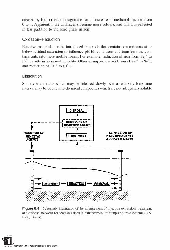
creased by four orders of magnitude for an increase of methanol fraction from0 to 1. Apparently, the anthracene became more soluble, and this was reflectedin less partition to the solid phase in soil.

Oxidation–Reduction

Reactive materials can be introduced into soils that contain contaminants at orbelow residual saturation to influence pH-Eh conditions and transform the con-taminants into more mobile forms. For example, reduction of iron from Fe3 toFe2 results in increased mobility. Other examples are oxidation of Se4 to Se6,and reduction of Cr4 to Cr3.

Dissolution

Some contaminants which may be released slowly over a relatively long timeinterval may be bound into chemical compounds which are not adequately soluble

Figure 8.8 Schematic illustration of the arrangement of injection extraction, treatment,and disposal network for reactants used in enhancement of pump-and-treat systems (U.S.EPA, 1992a).

Table 8.4 Advantages and Disadvantages of Injection Systems in Reactant-EnhancedPump-and-Treat Systems

Advantages Disadvantages

Fluid injectionmode

Continuous Fluid distributed over wide area Greater potential for clogging ofscreens

Less maintenance of pumping sched- Greater pumping costsules

Slug Less volume of water Fluid distributed over very small vol-ume of aquifer

Less potential clogging of wellsPulsed Can be developed around working Requires more design to ensure injec-

schedules tion and off periods are balanced rel-ative to natural groundwater flow

Active agentinjectionmodeContinuous Maintain concentration in high perme-

ability zones allowing for diffusioninto low-permeability zones

Slug Requires less mass of active agent May not allow sufficient time for diffu-sion into low-permeability lenses

Concentration decreases with time/dis-tance, which can reduce effective-ness of the active agent

Pulsed Less total mass of active agent Requires greater maintenance/controlCan be planned around work schedules Requires more analysis to ensure that

injection and off periods are of suf-ficient length

Allows for sufficient time for diffusion

Source: U.S. EPA (1992a).

under prevailing conditions. Particularly for soils that are contaminated by inor-ganic substances, modification of pH through the addition of substances such aslime and other materials that provide H for competition with metal ions forsorption sites can make contaminants more available for extraction.

In using reactive agents to enhance the effectiveness of pump-and-treat systems, several operational factors need to be assessed. Among thesefactors are the feasibility of recovering and reusing the reactive agent, the pos-sibility of interference of the reactive agent with the treatment processes forthe extracted water, the environmental and human toxicity of the reactiveagent, and the optimal method for introduction of the agent into the contam-

inated soil. A schematic illustration of the arrangement of injection and ex-traction points, and their links to treatment and disposal systems for both ex-tracted water and reactive agents, is provided in Figure 8.8. Fluids which carrythe reactive agent and the reactive agent itself may be injected using one of threeoptional modes: continuous, slug, and pulsed injection modes. The advantagesand disadvantages of each of these modes are summarized in Table 8.4 (afterU.S. EPA, 1992a)

8.5 IN-SITU SOIL FLUSHING

In-situ soil flushing is the injection of flushing solution to permeate soils to releasebound contaminants and move them with the infiltrating solution toward extrac-tion systems. As illustrated in Figure 8.9, the contaminated media to be treatedare usually located in the vadose zone. The flushing solution may be neutral ormay contain surface-active agents, some of which were discussed in Section 8.4.This treatment technique is usually designed for inorganic contaminants (metals)such as Pb, Cr, As, and Cd. In this process, the flushing solution infiltrates the

Figure 8.9 Illustration of a typical soil flushing system (U.S. EPA, 1997).

treatment zone and selectively extracts and displaces the target metals throughthe vadose zone into groundwater. Through pumping, the contaminated water isextracted and subjected to a treatment process in which the leached metal isprecipitated for disposal. In some cases, it may be necessary to inject a stabilizingsolution through residual media to fix the remaining substances.

Examples of substances that are commonly used in flushing solutions areHCL, EDTA, HNO3, and CaCl2. Leaching models such as those described inChapter 6 (Section 6.6) can be used to estimate the rate of displacement of con-taminants downward by percolating liquids. Detailed models for describing soilflushing have been published by Kayano and Wilson (1993) and Gabr et al.(1996). In general, soil flushing is effective in relatively permeable soils (siltsand sands).

8.6 VOLATILIZATION AND AIR PRESSURIZATIONPRINCIPLES

Extraction of contaminants from polluted media requires that the contaminantsbe made more available for transport out of the polluted media. The mobility ofcontaminants toward extraction points increases as they are transferred from thesolid phase of soil systems to the liquid phase and the gaseous phase, in thatorder. The objective of remediation schemes that are based on volatilization andair pressurization techniques is to induce the transfer of contaminants into soilatmosphere from which they can be more easily extracted than from the originalmedia.

8.6.1 In-Situ Soil Venting/Soil Vapor Extraction Principles

After the removal of free product from contaminated soils, the soil is unsaturatedwith contaminated liquid but the contaminant is still present in the residual liquid.In soil venting/soil vapor extraction, airflow through the contaminated zone isinduced through the application of a vacuum pressure, typically, through a welllocated in the center of the contaminated zone. Air inlet wells are then installedat the boundary of the zone. Application of vacuum pressure draws in air throughthe inlet wells and the contaminants that transfer from the soil and residual liquidsto the air are drawn out of the ground.

Efforts (Lingineni and Dhir, 1992; Johnson et al., 1990) have been madeto develop predictive models for the rate of contaminant removed for a givenset of contaminant properties, soil characteristics, vacuum pressures, and otheroperational features of soil venting systems. For the Johnson et al. (1990) analy-

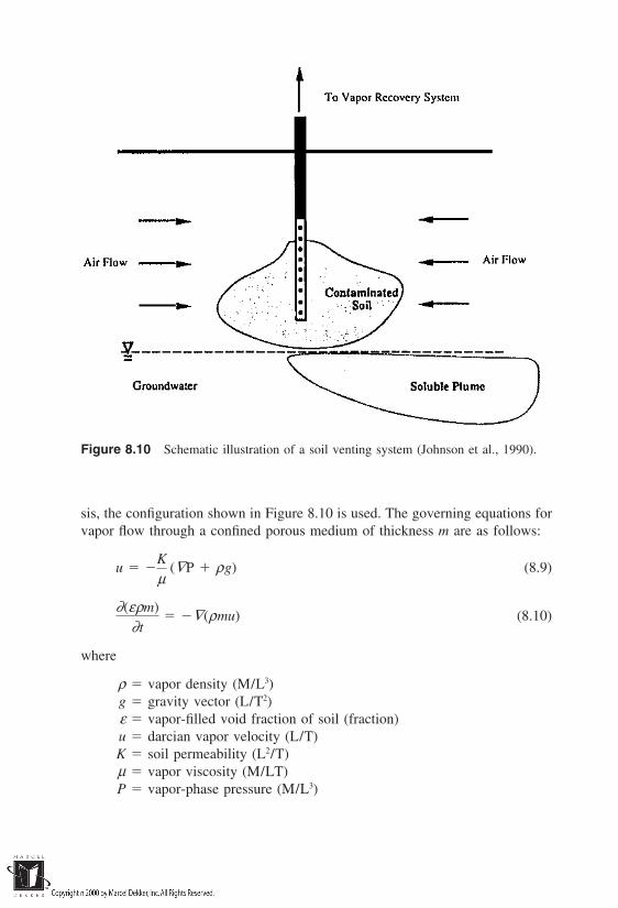
Figure 8.10 Schematic illustration of a soil venting system (Johnson et al., 1990).

sis, the configuration shown in Figure 8.10 is used. The governing equations forvapor flow through a confined porous medium of thickness m are as follows:

u K

µ(∇P ρg) (8.9)

∂(ερm)∂t

∇(ρmu) (8.10)

where

ρ vapor density (M/L3)g gravity vector (L/T2)ε vapor-filled void fraction of soil (fraction)u darcian vapor velocity (L/T)K soil permeability (L2/T)µ vapor viscosity (M/LT)P vapor-phase pressure (M/L3)

∇ gradient operator (1/T)m stratum thickness (L)

Equations (8.9) and (8.10) are Darcy’s law and the continuity equation,respectively. In Eq. (8.10), ρg can be neglected because vapor flow is consideredto be primarily in a direction that is orthogonal to gravity. Also, it will be assumedthat the soil permeability is affected by neither liquid removal nor by airflow. Inorder to establish the relationship between induced pressure and the density ofthe vapor, it is assumed herein that the vapor behaves as an ideal gas. Thus,

ρ ρatm P

Patm (8.11)

where

ρatm vapor density at reference pressure Patm (M/L3)

Equations (8.9) and (8.11) can be substituted into Eq. (8.10), resulting in thefollowing equation:

2εµK ∂P

∂t V2P (8.12)

Under conditions of steady state, radial flow with the boundary conditions P Pw, r Rw, and P Patm, r Ri, Eq. (8.12) can be solved as follows for ahomogeneous porous medium:

P2(r) P2w P2

atm P2w ln(r/Rw)

ln(ri/Rw) (8.13)

where

r nominal radius of the vacuum well (L)Pw pressure at the vaccum well of Rw (M/LT)Rw radius of the vaccum well (L)Ri radius of influence of the well (radius to where pressure is

equal to Patm) (L)Patm atmospheric pressure (M/LT)

Then, U(r), the radial Darcian velocity distribution and Q, the volumetric flowrate, can be calculated using the following equations:

u(r) K

2µ Pw(r/n(Rw/Ri))[1 (Patm/Pw)2]1 [1 (Patm/Pw)2][ln(r/Rw)]/[ln(Rw/Ri)]1/2 (8.14)

Q 2πRwu(Rw)H HπK

µ Pw[1 (Patm/Pw)2

ln(Rw/Ri) (8.15)

where

Q volumetric vapor flow rate (L3/T)H screened length of the vacuum well through the vadose

zone (L)

Considering that the soil system may be layered, an appropriate expression forsuch layered soils is given as Eq. (8.16)

Q n

i1

Qi (8.16)

where

Qi volumetric vapor flow rate through each homogeneous layer i(L3/T)

n number of homogeneous soil layers through which the screenedsegment of the vacuum well passes

Additional analyses for quantification of vapor extraction rates from soils areprovided by Bass (1993) and Gierke et al (1995).

The total mass of contaminant removed can be estimated as follows:

M QCat (8.17)

where

M cumulative mass of contaminant removed (M)Ca average concentration of contaminant in air (M/L3)

t time (T)

The average concentration Ca depends on the transfer of the contaminantfrom solid and liquid phases into vapor phase in the soil pores and the interactionof the vapor with the porous transport medium during its extraction. The relation-ship shown in Figure 8.11 is often observed between concentration and operationtime. The volatility of contaminants and the permeability of the soils are theprimary determinants of the effectiveness of soil vapor extraction systems (SVE).High permeability and high volatility enhance the effectiveness of SVE. In gen-eral, contaminants with vapor pressures greater than 0.5 mm Hg are consideredto be suitable for remediation using SVE (U.S. EPA, 1995). The Henry’s lawconstant is also a good indicator of volatility. It expresses the tendency of dis-solved contaminants to partition between the vapor and dissolved (in liquid)phases. Contaminants that have Henry’s law constant values in excess of 100 are

Figure 8.11 Relationship between contaminant concentration and extraction time insoil vapor extraction systems (U.S. EPA, 1995).

candidates for removal by SVE. Vapor pressures and Henry’s Law constant val-ues are provided for common constituents of petroleum in Tables 8.5 and 8.6,respectively.

8.6.2 In-Situ Steam Extraction Principles

In-situ steam extraction is an augmentation of the SVE process described in Sec-tion 8.6.1 through the injection of steam. The introduction of steam results inthe extraction of semivolatiles which would normally not be removed at lowertemperatures and drier conditions. This technology is useful for treating me-dia contaminated with chlorinated hydrocarbons, aromatics, alcohols, and high-boiling-point chlorinated aromatics. Figure 8.12 shows a typical configurationof an in situ steam extraction system.

8.6.3 In-Situ Air Sparging Principles

Unlike the SVE process, in which air is injected into the vadose zone (consistingof contaminated, unsaturated media), in air sparging, air is injected into the con-taminated soil below the water table. The injected air bubbles contact dissolvedand absorbed-phase contaminants and even NAPLs such that contaminants are

Table 8.5 Vapor Pressure of CommonPetroleum Constituents

Vapor pressureConstituent (mmHg at 20°C)

Methyl t-butyl ether 245Benzene 76Toluene 22Ethylene dibromide 11Ethylbenzene 7Xylenes 6Naphthalene 0.5Tetraethyl lead 0.2

Source: U.S. EPA (1995).

Table 8.6 Henry’s Law Constants ofCommon Petroleum Constituents

Henry’s lawConstituent constant (atm)

Tetraethyl lead 4700Ethylbenzene 359Xylenes 266Benzene 230Toluene 217Naphthalene 72Ethylene dibromide 34Methyl t-butyl ether 27

Source: U.S. EPA (1995).

transferred into them as they travel into the vadose zone. The oxygen introducedby injected air may increase the rate of biodegradation of in-situ contaminants.An air sparging system is illustrated schematically in Figure 8.12. As can beseen, air is introduced through the sparger well and contaminant-laden bubblestravel into the vadose zone, where they are removed by extraction wells. A moreelaborate illustration is shown in Figure 8.13.

The maximum concentration of contaminants in the air phase can be esti-mated as follows from the ideal gas law:

Figure 8.12 (a) Configuration of an in-situ steam extraction system (U.S. EPA, 1994a).(b) Schematic illustration of an air sparging system (U.S. EPA, 1996).

Figure 8.13 Schematic illustration of surface and subsurface components of an airsparging system (U.S. EPA, 1995).

Cm XiPiMi

RT(8.18)

where

Cm maximum vapor concentration in the vapor phase (mg/L)Xi mole fraction of component i in the liquid phase of the

contaminated mediaPi pure-component vapor pressure of component i at temperature

T (atm)Mi molecular weight of component i (mg/mole)R gas constant 0.0821 atm/mole-KT absolute temperature (K)

Air sparging is most effective for volatile contaminants in unstratified soils wheregroundwater contains little or no dissolved iron. Dissolved iron tends to oxidizein the presence of introduced oxygen and precipitate, thereby reducing the perme-ability of the soil to fluids. Air sparging is not recommended when the concentra-tion of Fe2 in groundwater exceeds 20 mg/L.

8.7 IN-SITU VITRIFICATION PRINCIPLES

Vitrification is the process by which materials (which may include waste-con-taining materials) are converted into glass or substances that behave like glass.

Considering that glass is a rigid, noncrystalline substance with very limited poros-ity, contaminants that are fused into glass are held tightly so that they may notleach out significantly.

In hazardous waste remediation practice, vitrification is usually inducedthrough heat application in situ, or the processing and heating of excavatedwastes. The latter enables greater control of the vitrification process but has thedisadvantage of greater human and environmental exposure risks if radioactiveand dispersive contaminants are involved. In this section, the focus is on theprinciples of in-situ vitrification. A vitrification process that is based on heatapplication may destroy organic contaminants through pyrolysis or combustion,and fuse inorganic metals, including radioactive elements into the structure ofglass. Glass is generally durable and has the capacity to incorporate a wide varietyof substances in a reasonably high range of concentrations. However, glass forma-tion requires that its component elements be available in appropriate forms andproportions. This is not always the case with contaminated media. Thus, someadditives may need to be added to deficient media to improve glass formation.During vitrification, both organic and inorganic substances may vaporize as off-gas, which often requires control or treatment.

Glass is composed of oxides of silicon (primary constituent), boron, alumi-num, and alkali and alkaline earth elements. The primary glass types that areused in waste vitrification processes are sodium silicates, borosilicates, and alumi-nosilicates. The following raw materials primarily supply the elements that areused in industrial glass formation. The mix proportions can be optimized to pro-duce glass of specific physicochemical characteristics.

Sand: SiO2

Limestone: CaCO3

Dolomite: CaMg(CO3)2

Soda ash: Na2CO3, KALSi3O8

The roles of various oxides in vitrification and performance of vitrified materialsis summarized in Table 8.7. The typical proportions of oxides in soda lime glass(used for making window glass), commercial borosilicate glass, and in-situ vitri-fied (ISV) glass are summarized in Table 8.8.

In contaminated media vitrification processes, the application of heat in thetemperature range of 1000–2000°C melts materials into a liquid. Upon cooling,the liquid solidifies into a largely noncrystalline (amorphous) mass. An illustra-tion of the in-situ heat application process in which electrodes are used is shownin Figure 8.14. The glass mass comprises a three-dimensional network of silicon–oxygen tetrahedra which lack crystallinity because of the irregularity and ran-domness of the silicon–oxygen bonds of the network. This structure is illustratedin Figure 8.15. Each silicon atom is bonded to four oxygen atoms which occupythe corners of the silicon–oxygen tetrahedra. Some or all of the oxygen atoms

Table 8.7 Effects of Waste-Glass Components on Processing and Performance ofVitrified Materials

Processing Product Performance

Frit ComponentsSiO2 Increases viscosity greatly; re- Increases durability

duces waste solubilityB2O3 Reduces viscosity; increases Increases durability in low

waste solubility amounts, reduces in largeamounts

Na2O Reduces viscosity and resistivity; Reduces durabilityincreases waste solubility

Li2O Same as Na2O, but greater effect; Reduces durability, but less thanincreases tendency to devitrify Na2O

K2O Same as Na2O; decreases ten- Reduces durability more thandency to devitrify Na2O

CaO Increases then reduces viscosity Increases then reduces durabilityand waste solubility

MgO Is same as CaO; reduces tendency Is same as CaO, but more likelyto vitrify to decrease durability

TiO2 Reduces viscosity slightly; in- Increases durabilitycreases then reduces waste solu-bility; increases tendency to de-vitrify

ZrO2, La2O3 Reduces waste solubility Increases durability greatly

Waste ComponentsAl2O3 Increases viscosity and has ten- Increases durability

dency to devitrifyFe2O3 Reduces viscosity; is hard to dis- Increases durability

solveU3O8 Reduces tendency to devitrify Reduces durabilityNiO Is hard to dissolve; increases ten- Reduces durability

dency to devitrifyMnO Is hard to dissolve Increases durabilityZeolite Is slow to dissolve; produces Increases durability

foamSulfate Is an antifoam, melting aid; in- Too much causes foam or forma-

creases corrosion of processing tion of soluble second phaseequipment

Source: Adapted from U.S. EPA (1992), originally developed by Plodinec et al. (1982).

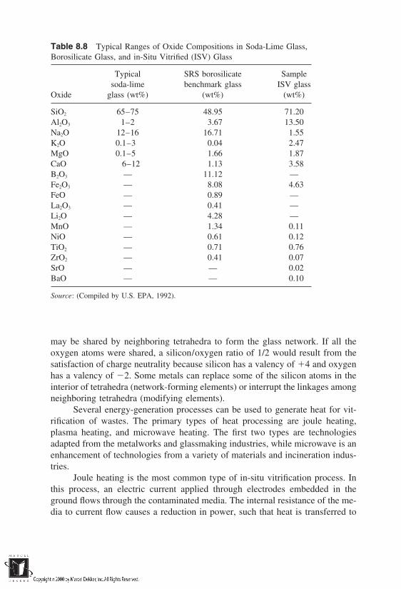
Table 8.8 Typical Ranges of Oxide Compositions in Soda-Lime Glass,Borosilicate Glass, and in-Situ Vitrified (ISV) Glass

Typical SRS borosilicate Samplesoda-lime benchmark glass ISV glass

Oxide glass (wt%) (wt%) (wt%)

SiO2 65–75 48.95 71.20Al2O3 1–2 3.67 13.50Na2O 12–16 16.71 1.55K2O 0.1–3 0.04 2.47MgO 0.1–5 1.66 1.87CaO 6–12 1.13 3.58B2O3 — 11.12 —Fe2O3 — 8.08 4.63FeO — 0.89 —La2O3 — 0.41 —Li2O — 4.28 —MnO — 1.34 0.11NiO — 0.61 0.12TiO2 — 0.71 0.76ZrO2 — 0.41 0.07SrO — — 0.02BaO — — 0.10

Source: (Compiled by U.S. EPA, 1992).

may be shared by neighboring tetrahedra to form the glass network. If all theoxygen atoms were shared, a silicon/oxygen ratio of 1/2 would result from thesatisfaction of charge neutrality because silicon has a valency of 4 and oxygenhas a valency of 2. Some metals can replace some of the silicon atoms in theinterior of tetrahedra (network-forming elements) or interrupt the linkages amongneighboring tetrahedra (modifying elements).

Several energy-generation processes can be used to generate heat for vit-rification of wastes. The primary types of heat processing are joule heating,plasma heating, and microwave heating. The first two types are technologiesadapted from the metalworks and glassmaking industries, while microwave is anenhancement of technologies from a variety of materials and incineration indus-tries.

Joule heating is the most common type of in-situ vitrification process. Inthis process, an electric current applied through electrodes embedded in theground flows through the contaminated media. The internal resistance of the me-dia to current flow causes a reduction in power, such that heat is transferred to

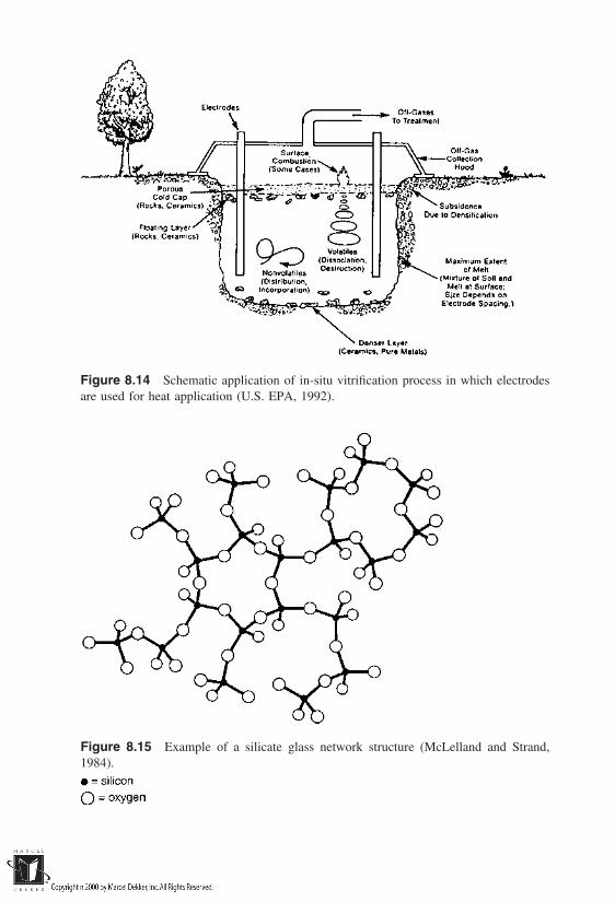
Figure 8.14 Schematic application of in-situ vitrification process in which electrodesare used for heat application (U.S. EPA, 1992).

Figure 8.15 Example of a silicate glass network structure (McLelland and Strand,1984).

the media. Joule’s law provides a quantitative method for estimating the powerthat is dissipated in the media:

P I2R (8.19)

R V

I(8.20)

where

P dissipated power (watts)I current flow through the media (amperes)

R resistance of the material (ohms)V voltage across the material (volts)

Generally, soils are very resistant because of the low electrical conductivityof SiO2, its primary constituent. However, soils are less resistant at higher temper-atures. Initially, high voltage in the regime of 2000–4000 volts is applied tocompensate for the soil’s high resistance at low temperatures. In addition, flakedgraphite and glass frit are placed between electrodes to reduce the initial conduc-tivity of soils to initiate soil heating. These enhancers are subsequently destroyedat higher temperatures and the heat in the system reaches levels at which soil isheated more efficiently. In this later stage high voltage is no longer necessaryand can be reduced by as much as 10-fold.

In plasma heating (which is currently mostly ex-situ), heat is producedthrough conversion of a gas to plasma under energy supplied by an electric arcgenerated by direct current (DC) or alternating current (AC) sources. Essentially,a plasma is an ionized gas, typically produced from materials such as oxygen,nitrogen, air, noble gases, or their mixtures. The process is used because ionizedmaterials are good conductors of electricity. A column of the gas(es) is heated inthe equipment and heat is produced and transferred to the soil through convection,radiation, and electrical resistance.

In microwave heating, which is currently an ex-situ process, the contami-nated media absorb electromagnetic radiation in the effective microwave range(3000–30,000 MHz). The radiation is directed into the contaminated mediathrough waveguides. Soils are dielectric materials, implying that they are noteffective conductors of heat. Dielectrics exhibit some polarization under an elec-tric field. Alternation of the field causes distortion of the molecules of dielectricmaterials (Orfeuil, 1987), resulting in heating of the material. This is the principlethat underlies the use of microwave for heating of soils to vitrified masses.

The vitrification processes described in the preceding sections result in thefollowing vitrification treatment mechanisms for contaminants:

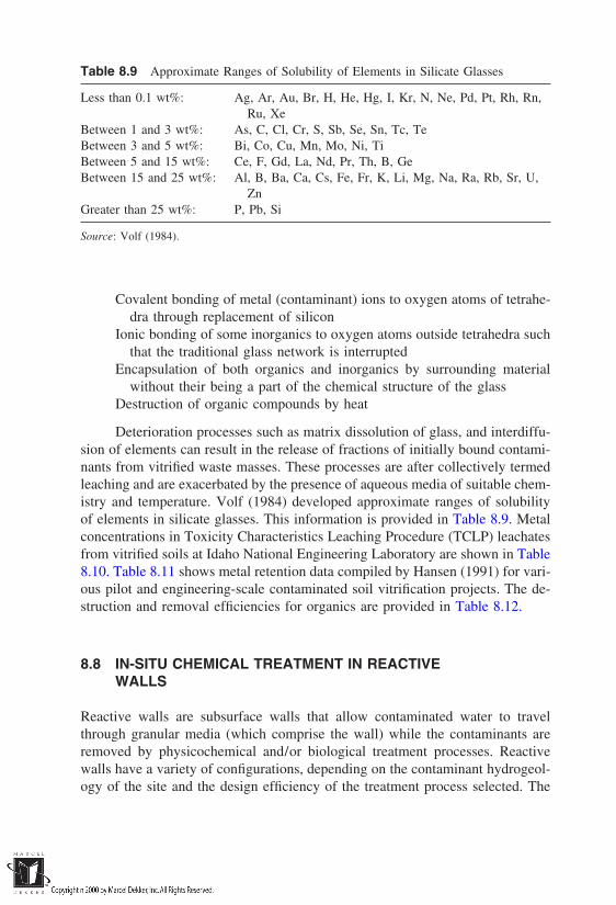
Table 8.9 Approximate Ranges of Solubility of Elements in Silicate Glasses

Less than 0.1 wt%: Ag, Ar, Au, Br, H, He, Hg, I, Kr, N, Ne, Pd, Pt, Rh, Rn,Ru, Xe

Between 1 and 3 wt%: As, C, Cl, Cr, S, Sb, Se, Sn, Tc, TeBetween 3 and 5 wt%: Bi, Co, Cu, Mn, Mo, Ni, TiBetween 5 and 15 wt%: Ce, F, Gd, La, Nd, Pr, Th, B, GeBetween 15 and 25 wt%: Al, B, Ba, Ca, Cs, Fe, Fr, K, Li, Mg, Na, Ra, Rb, Sr, U,

ZnGreater than 25 wt%: P, Pb, Si

Source: Volf (1984).

Covalent bonding of metal (contaminant) ions to oxygen atoms of tetrahe-dra through replacement of silicon

Ionic bonding of some inorganics to oxygen atoms outside tetrahedra suchthat the traditional glass network is interrupted

Encapsulation of both organics and inorganics by surrounding materialwithout their being a part of the chemical structure of the glass

Destruction of organic compounds by heat

Deterioration processes such as matrix dissolution of glass, and interdiffu-sion of elements can result in the release of fractions of initially bound contami-nants from vitrified waste masses. These processes are after collectively termedleaching and are exacerbated by the presence of aqueous media of suitable chem-istry and temperature. Volf (1984) developed approximate ranges of solubilityof elements in silicate glasses. This information is provided in Table 8.9. Metalconcentrations in Toxicity Characteristics Leaching Procedure (TCLP) leachatesfrom vitrified soils at Idaho National Engineering Laboratory are shown in Table8.10. Table 8.11 shows metal retention data compiled by Hansen (1991) for vari-ous pilot and engineering-scale contaminated soil vitrification projects. The de-struction and removal efficiencies for organics are provided in Table 8.12.

8.8 IN-SITU CHEMICAL TREATMENT IN REACTIVEWALLS

Reactive walls are subsurface walls that allow contaminated water to travelthrough granular media (which comprise the wall) while the contaminants areremoved by physicochemical and/or biological treatment processes. Reactivewalls have a variety of configurations, depending on the contaminant hydrogeol-ogy of the site and the design efficiency of the treatment process selected. The

Table 8.10 TCLP Extract Metal Concentrations in Leachate from Idaho NationalEngineering Laboratory Vitrified Soils

Maximum Vitrifiedallowable Contaminated productleachate soil leachate

concentration concentration concentrationMetal (mg/liter) (mg/kg) (mg/liter)

Arsenic 5.0 200 0.168Barium 100.0 200 0.229Cadmium 1.0 200 0.0098Chromium 5.0 200 0.0178Lead 5.0 2000 0.636Mercury 0.2 200 0.0001Selenium 1.0 200 0.098Silver 5.0 200 0.023

Source: U.S. EPA (1994b).

most basic design involves funneling groundwater through one or more gatesinto one or multiple reaction zones. The system is designed such that the exitconcentration Ce of the target contaminant is adequately reduced, relative to theentry concentration, Co. Sampling points are usually placed in both the entry andexit zones of the wall as well as along the flow axis within the wall, to monitorcontaminant concentrations in space and time. Schematic illustrations of reactivewalls are shown in Figs. 8.16 and 8.17. Reactive walls can be placed in seriesor in parallel to achieve contaminated water treatment efficiencies or provide a‘‘treatment train’’ in which each wall targets a different contaminant within thepolluted groundwater.

Essentially, the wall is an in-situ reactor that can operate using one or moretreatment process to transform and/or remove contaminants. The prevailing pro-cesses depend on the type of packing material and additives used in the wall.Commonly, earthen media such as fine sands and silts are mixed with reactivesubstances or coated with the latter such that adequate permeability can be main-tained while reactions that occur at estimated rates are sustained. The choice ofreactive media and other design elements is made to ensure that contaminatedwater residence time within the treatment zone is long enough for significantreactions to occur. With respect to typical dimensions, one system described byO’Hannesin and Gillham (1993) has a length of 5.5 m, a thickness of 1.6 m, andwas located at a depth of 2.2m below the groundsurface and 1.0 m below thewater table. Examples of reactive substances that can be used in reactive walls arezero-valent iron (iron filings), limestone, organic carbon, and microbial consortia.

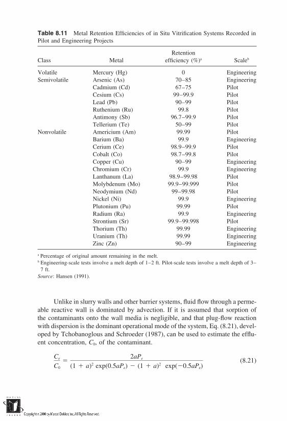
Table 8.11 Metal Retention Efficiencies of in Situ Vitrification Systems Recorded inPilot and Engineering Projects

RetentionClass Metal efficiency (%)a Scaleb

Volatile Mercury (Hg) 0 EngineeringSemivolatile Arsenic (As) 70–85 Engineering

Cadmium (Cd) 67–75 PilotCesium (Cs) 99–99.9 PilotLead (Pb) 90–99 PilotRuthenium (Ru) 99.8 PilotAntimony (Sb) 96.7–99.9 PilotTellerium (Te) 50–99 Pilot

Nonvolatile Americium (Am) 99.99 PilotBarium (Ba) 99.9 EngineeringCerium (Ce) 98.9–99.9 PilotCobalt (Co) 98.7–99.8 PilotCopper (Cu) 90–99 EngineeringChromium (Cr) 99.9 EngineeringLanthanum (La) 98.9–99.98 PilotMolybdenum (Mo) 99.9–99.999 PilotNeodymium (Nd) 99–99.98 PilotNickel (Ni) 99.9 EngineeringPlutonium (Pu) 99.99 PilotRadium (Ra) 99.9 EngineeringStrontium (Sr) 99.9–99.998 PilotThorium (Th) 99.99 EngineeringUranium (Th) 99.99 EngineeringZinc (Zn) 90–99 Engineering

a Percentage of original amount remaining in the melt.b Engineering-scale tests involve a melt depth of 1–2 ft. Pilot-scale tests involve a melt depth of 3–

7 ft.Source: Hansen (1991).

Unlike in slurry walls and other barrier systems, fluid flow through a perme-able reactive wall is dominated by advection. If it is assumed that sorption ofthe contaminants onto the wall media is negligible, and that plug-flow reactionwith dispersion is the dominant operational mode of the system, Eq. (8.21), devel-oped by Tchobanoglous and Schroeder (1987), can be used to estimate the efflu-ent concentration, C0, of the contaminant.

Ce

C0

2aPe

(1 a)2 exp(0.5aPe) (1 a)2 exp(0.5aPe)(8.21)

Table 8.12 Organics Destruction and Removal Efficiencies (DRE) Recorded forContaminated Media Vitrification Systems (HWC, 1990)

Initial Total DREconcentration Percent (including

Contaminant (ppb) destruction off-gas removal)

Aldrin 113 97 99.99Chlordane 535,000 99.95 99.999DDD, DDE, DDT 21–240,000 99.9–99.99 99.999Dieldrin 24,000 98–99.9 99.99Dioxins 47,000 99.9–99.99 99.9999Fuel Oils 230–11,000 99 99.999Furans 9,400 99.9–99.99 99.9999Glycol NA 90 99.99Heptachlor 61 98.7 99.99MEK NA 99 99.999PCBs 19,400,000 99.9–99.99 99.9999Pentachlorophenol 4,000,000 99.995 99.99999Toluene 203,000 99.996 99.99999Trichloroethane 106,000 99.995 99.99999Xylenes 3,533,000 99.998 99.99999

Source: Hazardous Waste Consultant (HWC) (1990).

Figure 8.16 Funnel-and-gate configuration of a reactive wall for in-situ treatment ofcontaminated groundwater.

Figure 8.17 Array of monitoring points for assessing the effectiveness of a double-gate reactive wall treatment system.

a (1 4λtPe)0.5 (8.22)

Pe vL

D(8.23)

where

Ce exit concentration of the contaminant (M/L3)C0 entrance concentration of the contaminant (M/L3)Pe Peclet number (unitless)L length of the treatment zone (L)ν contaminated water flow velocity (L/T)D dispersion coefficient of the contaminant through the wall

(L2/T)λt decay rate constant of the target contaminant (I/T)

Most commonly, reactive walls in full-scale and bench-scale projects applycontaminant transformation processes (oxidation and reduction for organics) andprecipitation of inorganic compounds through modification of Eh and pH condi-tions. Iron metal and iron compounds have been used to degrade hydrocarbonsand precipitate some metals. In particular, dehalogenation of chlorinated solventshas been accomplished through the use of reduced forms of iron such as Fe0,

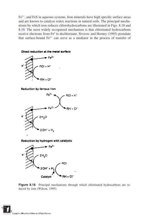
Fe2, and FeS in aqueous systems. Iron minerals have high specific surface areasand are known to catalyze redox reactions in natural soils. The principal mecha-nisms by which iron reduces chlorohydrocarbons are illustrated in Figs. 8.18 and8.19. The most widely recognized mechanism is that chlorinated hydrocarbonsreceive electrons from Fe0 to dechlorinate. Sivavec and Horney (1995) postulatethat surface-bound Fe2 can serve as a mediator in the process of transfer of

Figure 8.18 Principal mechanisms through which chlorinated hydrocarbons are re-duced by iron (Wilson, 1995).

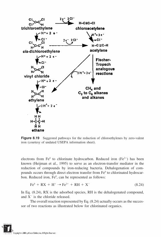
Figure 8.19 Suggested pathways for the reduction of chloroethylenes by zero-valentiron (courtesy of undated USEPA information sheet).

electrons from Fe0 to chlorinate hydrocarbon. Reduced iron (Fe2) has beenknown (Heijman et al., 1995) to serve as an electron-transfer mediator in thereduction of compounds by iron-reducing bacteria. Dehalogenation of com-pounds occurs through direct electron transfer from Fe0 to chlorinated hydrocar-bon. Reduced iron, Fe0, can be represented as follows:

Fe0 RX H Fe2 RH X (8.24)

In Eq. (8.24), RX is the adsorbed species, RH is the dehalogenated compound,and X is the chloride released.

The overall reaction represented by Eq. (8.24) actually occurs as the succes-sor of two reactions as illustrated below for chlorinated organics.

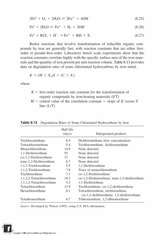
2Fe0 O2 2H2O s 2Fe2 4OH (8.25)

Fe0 2H2O s Fe2 H2 2OH (8.26)

Fe0 RCL H Fe2 RH X (8.27)

Redox reactions that involve transformation of reducible organic com-pounds by iron are generally fast, with reaction constants that are either first-order or pseudo-first-order. Laboratory bench scale experiments show that thereaction constants correlate highly with the specific surface area of the iron mate-rials and the quantity of iron present per unit reaction volume. Table 8.13 providesdata on degradation rates of some chlorinated hydrocarbons by iron metal.

K (M Xm)S (C Xc)

where

K first-order reaction rate constant for the transformation oforganic compounds by iron-bearing materials (I/T)

M central value of the correlation constant slope of K versus Sline (L/T)

Table 8.13 Degradation Rates of Some Chlorinated Hydrocarbons by Iron

Half-life(days) Halogenated products

Trichloromethane 6.5 Dichloromethane (low concentration)Tetrachloromethane 5.4 Trichloromethane, dichloromethaneMonochloroethene 14.9 None detected1,1-Dichloroethene 55 None detectedcis-1,2-Dichloroethene 37 None detectedtrans-1,2-Dichloroethene 6.7 None detected1,1,1-Trichloroethane 5.5 1,1-Dichloroethane1,1,2-Trichloroethane 7.8 Trace of monochloroetheneTrichloroethene 7.1 cis-1,2-Dichloroethene1,1,2,2-Tetrachloroethane 10.2 cis-1,2-Dichloroethene, trans-1,2-dichlorethene1,1,1,2-Tetrachloroethane 5.2 1,1-DichloretheneTetrachloroethene 13.9 Trichloroethene, cis-1,2-dichloroetheneHexachloroethane 6.1 Tetrachloroethene, trichloroethene,

cis-1,2-dichloroethene, 1,2-dichloroethaneTetrabromoethene 6.7 Tribromoethene, 1,2-dibromoethene

Source: Developed by Wilson (1995), using U.S. EPA information.

Xm numerical bounds of the range of the correlation constant aboutits average

S total surface area of iron-bearing material per unit reactionvolume (L2/L3)

C correlation constant representing intercept of the trend line onthe K axis (I/T)

Xc upper or lower limit of C (I/T)

For chloroethenes (chlorinated ethenes) reduced by iron metal (Fe0) in batchexperiments conducted (Sivavec and Horney, 1995) at 25°C, K values are sum-marized in Table 8.14. The magnitudes of the correlation parameters are

M 1.27 104 m/hXm 2.40 105 m/hC 8.45 103 h1

Xc 3.67 10 3 h1

For dechlorination of TCE (a chloroethene) by iron sulfide (FeS), Sivavecet al. (1995) obtained the following values:

M 8.68 104 m/hXm not applicableC 7.16 104 h1

Xc not applicable

Table 8.14 Reductive Dechlorination Rates of Aqueous Chlorinated EthenesDetermined in Batch Experiments at 25°C (Milli-Q water buffered with 40 mg/literCaCO3, initial pH 7) (25.0 g VWR untreated iron filings: 122 mg/liter aq PCE,TCE, DCE, or VC)

Initial Iron surfaceconc. area/volume Rate

Chloroethene (mg/liter) (m2/liter) constant (h1) t1/2 (h) r2

PCE 20.0 254 0.0549 13 0.990TCE 19.2 254 0.0746 9 0.963cis-DCE 22.2 254 0.0037 187 0.837trans-DCE 22.9 254 0.0257 27 0.9921,1-DCE 21.6 254 0.0047 147 0.615VC 23.6 254 0.0039 177 0.910

Source: Sivavec and Horney (1995).

Figure 8.20 Effects of zero-valent iron metal surface area concentration on pseudo-first-order reaction rate constant for nitrobenzene reduction (Agrawal and Tratnyek,1996).

For reduction of nitrobenzene by Fe0, Agrawal and Tratnyek (1996) ob-tained the following data. The trend line is shown in Figure 8.20, noting that forthe following data, K is in 1/min, and S is in M2/liter.

M 3.90 103 m/minXm 2.00 103 m/minC 3.00 103 min1

Xc 1.00 103 min1

Studies by Chuang et al. (1995) have indicated that Fe0 can promote thedechlorination of polychlorinated biphenyls (PCBs) without a solvent at tempera-tures in the regime of 400–500°C. However, the reader should note that greatercontrol of experimental conditions can be maintained in the laboratory thanwithin the subsurface environment in which reactive walls are designed to op-erate.

8.9 SOLIDIFICATION/STABILIZATION (EX-SITU)PRINCIPLES

Solidification and stabilization are waste treatment processes that are intendedprimarily to reduce the mobility of waste constituents. Solidification is the changein waste physical state, from a nonsolid to a solid. Stabilization is the modificationof the waste such that it is converted to a less soluble, mobile or toxic form.Thus, solidification/stabilization of waste materials, which is usually performedex-situ following adaptations of the treatment scheme illustrated in Figure 8.21,has the following advantages.

1. Improvement in waste handling due to possible reduction in volume2. Decrease in the surface area of waste available for leaching of contami-

nants3. Reduction in the solubility of waste4. Transformation of contaminants in waste from toxic to nontoxic forms.

The reader should note that regardless of the possibility of occurrence of advan-tages 3 and 4, solidification/stabilization (S/S) is considered to be primarily aphysical treatment technique for wastes.

In the following paragraphs, the primary types of stabilization and theirbasic principles are described.

Figure 8.21 Schematic illustration of the solidification/stabilization process for con-taminated media (courtesy of U.S. EPA).

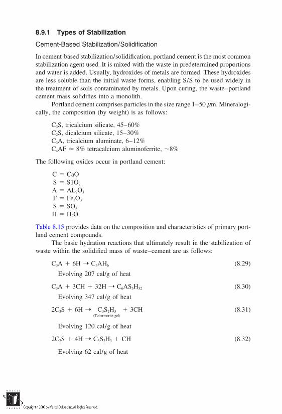
8.9.1 Types of Stabilization

Cement-Based Stabilization/Solidification

In cement-based stabilization/solidification, portland cement is the most commonstabilization agent used. It is mixed with the waste in predetermined proportionsand water is added. Usually, hydroxides of metals are formed. These hydroxidesare less soluble than the initial waste forms, enabling S/S to be used widely inthe treatment of soils contaminated by metals. Upon curing, the waste–portlandcement mass solidifies into a monolith.

Portland cement comprises particles in the size range 1–50 µm. Mineralogi-cally, the composition (by weight) is as follows:

C3S, tricalcium silicate, 45–60%C2S, dicalcium silicate, 15–30%C3A, tricalcium aluminate, 6–12%C4AF 8% tetracalcium aluminoferrite, 8%

The following oxides occur in portland cement:

C CaOS S1O2

A AL2O3

F Fe2O3

S SO3

H H2O

Table 8.15 provides data on the composition and characteristics of primary port-land cement compounds.

The basic hydration reactions that ultimately result in the stabilization ofwaste within the solidified mass of waste–cement are as follows:

C3A 6H C3AH6 (8.29)

Evolving 207 cal/g of heat

C3A 3CH 32H C6AS3H32 (8.30)

Evolving 347 cal/g of heat

2C3S 6H C3S2H3(Tobermorite gel)

3CH (8.31)

Evolving 120 cal/g of heat

2C2S 4H C3S2H3 CH (8.32)

Evolving 62 cal/g of heat

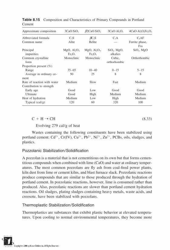
Table 8.15 Composition and Characteristics of Primary Compounds in PortlandCement

Approximate composition 3CaO⋅SiO2 β2CaO⋅SiO2 3CaO⋅Al2O3 4CaO⋅Al2O3Fe2O3

Abbreviated formula C3S βC2S C3A C4AFCommon name Alite Belite — Ferrite phase,

FssPrincipal MgO, Al2O3, MgO, Al2O3, SiO2, MgO, SiO2, MgO

impurities Fe2O3 Fe2O3 alkaliesCommon crystalline Monoclinic Monoclinic Cubic, Orthorhombic

form orthorhombicProportion present (%)

Range 35–65 10–40 0–15 5–15Average in ordinary ce- 50 25 8 8

mentRate of reaction with water Medium Slow Fast MediumContribution to strength

Early age Good Low Good GoodUltimate Good High Medium Medium

Heat of hydration Medium Low High MediumTypical (cal/g) 120 60 320 100

C H CH (8.33)

Evolving 279 cal/g of heat

Wastes containing the following constituents have been stabilized usingportland cement: Cd2, Cr(IV), Cu2, Pb2, Ni2, Zn2, PCBs, oils, sludges, andplastics.

Pozzolanic Stabilization/Solidification

A pozzolan is a material that is not cementitious on its own but that forms cemen-titious compounds when combined with lime (CaO) and water at ordinary temper-atures. The most common pozzolans are fly ash from coal-fired power plants,kiln dust from lime or cement kilns, and blast furnace slack. Pozzolanic reactionsproduce compounds that are similar to those produced through the hydration ofportland cement. In pozzolanic reactions, however, lime is consumed rather thanproduced. Also, pozzolanic reactions are slower than portland cement hydrationreactions. Oil sludges, plating sludges containing heavy metals, waste acids, andcreosote, have been stabilized with pozzolans.

Thermoplastic Stabilization/Solidification

Thermoplastics are substances that exhibit plastic behavior at elevated tempera-tures. Upon cooling to normal environmental temperatures, they become more

solid (tougher). In contaminated media treatment applications, they are used inmicroencapsulations in which the thermoplastic occupies pore spaces amongwaste/soil particles. Examples of commonly used thermoplastics are asphalt (bi-tumen) and polyethylene. Microencapsulation, which is essentially a physicaltreatment technique, can result in waste volume reduction and easier handling,elimination of free liquids from waste, lower permeability, and increased strengthof the waste matrix. The disadvantages are that it has a high air pollution potential,high sensitivity to organics and salt content, and requires the use of expensiveequipment.

Macroencapsulation

Macroencapsulation is the enclosure of contaminated media or waste within over-pack materials and containers. The waste or contaminated media may be microen-capsulated before macroencapsulation. Usually, drums of encapsulated wastesare produced in this process. Examples of wastes that are usually considered formacroencapsulation are incinerator ash, polychlorinated biphenyls (PCBs), anddioxins.

8.9.2 Performance Analysis for Stabilized/SolidifiedWastes

Stabilized/solidified materials usually need to be analyzed with respect to theirdurability and the associated potential for release of contaminants into environ-mental media. This is born of the concern that water (whether through precipita-tion or groundwater) and air will eventually have the opportunity to contact thestabilized/solidified media and thus promote the release of materials through pro-cesses of leaching. Although stabilized media strength and durability are some-times assessed, contaminant leachability is the primary issue in performance eval-uation of S/S wastes. It should be noted that the leachability discussion providedin this section also applies to other treated wastes.

Leachability is the release of contaminants from waste matrix into the aque-ous phase and the exit of these contaminants from the bounding surfaces of thewaste mass. Several direct and indirect factors influence contaminant leachabilityfrom a stabilized matrix. These factors are discussed below.

Surface Area of the Waste

Typically, contaminant leachability increases with the specific surface of particu-late media. The specific surface is the ratio of total available surface area to thewaste mass volume or weight. The specific surface increases from that of a mono-lith, through that of a granular mass, to the highest level in fine powders, for thesame external volume or weight of a material.

For a regularly shaped monolith, the specific surface is easily computedbecause internal porosity is not taken into account in the estimation of its surfacearea. For a mass of granular materials or fine powders that comprises varioussize fractions, internal and intergranular porosity and particle size distributionhave to be taken into consideration. The volumetric specific surface, Sf of suchmaterials can be computed as follows for a particulate medium that comprisesidealized spherical particles of various size fractions:

Sf As

V(8.34)

Sf volumetric specific surface (1/L)As surface area of particles within the waste mass (L2)V external volume of the waste mass (L3)

It should be noted that V is not the summation of the volumes of individualparticles of the waste mass. If this is done, the incorrect assumption is that theparticulate medium, consisting of various particle sizes, has a porosity of zero.The volumetric specific surface, Sf can be further computed as follows:

Sf

m

i1

4πr2i Ni

m

i1

[1.333πri3Ni/(1 n)](8.35)

Sf 3(1 n)m

i1fi

ri (8.36)

Sf 3(1 n)

ra

(8.37)

where

ri representative radius (possibly average) of the ith particlefraction of the medium (L)

Ni number of particles in the ith fraction of the medium (unitlessnumber)

n intergranular porosity of the medium (unitless fraction)fi volume fraction of the ith particle size in the medium (unitless

fraction)ra harmonic mean radius of all particles in the medium (L)

Agitation Technique and Equipment

In laboratory tests, agitation is necessary to accelerate the attainment of equilib-rium between solid samples and leachant. Contaminant leachability tends to bedirectly proportional to the intensity of agitation due to particle breakage (andhence increased specific surface) and leachant renewal at the waste solid–leachant interface.

Characteristics of the Leachant

The pH and Eh of the leachant affect contaminant leachability because of theircontrols on the solubility of compounds within the waste matrix. Some mineralsand contaminants are more stable within the waste matrix at specific ranges ofleachant pH and Eh, while they are less stable at other ranges. In the field, theseparameters may fluctuate with time.

Leachant/Waste Volumetric Ratio

The higher the leachant/waste volumetric ratio, the higher is the total mass ofcontaminant released for a given time interval, although recorded concentrationsof the leached contaminant may be less than those for lower leachant/waste volu-metric ratios within the same time envelope. Field ratios are difficult to simulatein the laboratory because of the intermittent manner in which the leachant issupplied by rainfall and other sources over an extended time period.

Duration of Contact

The longer the duration of contact of the leachant with the waste, the greater isthe opportunity for contaminant removal. Some waste constituents can only beremoved when associated mineral phases have dissolved. Dissolution of suchminerals may require a minimum duration under prevailing environmental condi-tions.

Temperature Conditions

The solubilities of most substances tend to be directly proportional to tempera-ture, although it should be noted that solubility is not the sole determinant of themagnitude of leaching. Upon dissolution, the contaminant species must find theirway (through diffusion or other transport processes) to the boundary throughwhich they pass to establish leaching rates. The media through which this trans-port occurs (which may be the waste or stabilized waste itself) have various levelsof permeability, dispersion, and diffusion constants with respect to the travelingcontaminant species.

Number of Elutions of Leachate

Within a given time interval, the greater the number of elutions, the larger is thetotal quantity of contaminants leached (with the total available quantities of thecontaminants in the waste being the upper-bound values). For most contaminants,after reaching a maximum, the concentration of the contaminant in the leachatedecreases for each subsequent elution. This often follows a negative exponentialpattern of concentration decrease. Essentially, as the pore fluid (leachant) receivesmore and more contaminant by diffusion from the waste matrix, the concentrationgradient between the waste matrix and the leachant decreases, resulting in re-duced transfer rate. If the contaminant-laden pore fluid is purged (eluted) and itsconcentration measured, the value obtained is usually less than that of subsequentelutions because for the latter, less and less of the contaminant is available inthe matrix for leaching.

Upon rising to a maximum value, M0, the concentration of a target contami-nant in the leachate usually follows equation (8.38).

Mt M0 exp(kt) (8.38)

where

Mt contaminant concentration in leachant measured at time ornumber of elutions t (M/L3)

M0 contaminant concentration in leachant at reference time ornumber of elutions, t0 (M/L3)

k empirical leaching constant obtainable from laboratory tests(unitless number)

t time (T) or number of elutions

8.9.3 Tests for Leachability Assessment

Several empirical tests that exhibit different levels of simulative capacity forwaste leachability in the field have been developed to evaluate stabilized, solidi-fied wastes, wastes treated using other methods, and untreated wastes (often forclassification and treatment process selection purposes). The results obtainedfrom laboratory tests for S/S wastes using a specific type of test depend on thefollowing two sets of factors:

1. The simulative capacity of the test variables to field conditions, interms of the factors discussed in the previous section.

2. The effectiveness of the S/S technique

The most common leachability assessment tests are described briefly below.

Toxicity Characteristics Leaching Procedure (TCLP) Test

The TCLP is a batch test conducted on samples that are crushed to a maximumparticle size of 9.5 mm. Liquids are usually separated from solids before useof the solids in the test. The leaching solution is added to the waste in a zeroheadspace extractor (ZHE) at a liquid:solid ratio of 20:1. The sample is thenagitated in a rotary tumbler at 30 rpm for 18 h. The leaching solution is filtered outand combined with the free liquid that had been separated earlier. Contaminantconcentrations are then measured. The TCLP test is mostly suitable for wasteclassification. Unless obtained concentrations are modified, the results lack thesimulative capacity needed for extension of its utility to contaminant source-termand transport assessments for field scenarios.

Extraction Procedure Toxicity (EP TOX) Test

The EP TOX test is similar to the TCLP test except that the pH of the leachantis periodically adjusted up to a specified maximum acid addition. It should benoted that for the TCLP test, the acid is added only once: at the onset of the test.EP TOX tests tend to extract lesser concentrations of metals from media thanTCLP tests because on a total basis the conditions (of the EP TOX tests) are lessaggressive, as shown in Table 8.16.

Monofill Waste Extraction Procedure (MWEP)

The MWEP test, which was formerly called the Solid Waste Leach Test, involvesmultiple extractions of leachate from a monolith or crushed mass of waste usingdistilled/deionized water. Usually, the sample is tested as a monolith if it passesa structural integrity test (for strength); otherwise, it is crushed until all particles

Table 8.16 Comparison of TCLP and EP TOX Test Parameters

Experimental parameter TCLP EP TOX

Filter size, µm 0.6–0.8 0.45Filter pressure, psi 50 75Leaching solution Acetate buffered Acetic acid

solution (pH 3 or 5) (pH 5)Period of extraction, h 18 24Liquid:solid ratio 20:1 16:1

Source: U.S. EPA (1989b).

pass a 9.5-mm sieve before use in batch testing. Leaching conditions are consid-ered to be mild: a liquid:solid ratio of 10:1, operated for 18 h per extraction,using nonacidic leachant.

Multiple Extraction Procedure (MEP)

In the MEP test, contaminants are sequentially extracted from a material usinga synthetic acid rain solution. This test is useful for addressing the effects ofleachant pH changes on contaminant leachability from waste samples. Usually,acetic acid solution is used for the first extraction, followed with a concentratedH2SO4/HNO3 solution (proportion of 60%/40% by weight) that is diluted to apH of 3.0. In total, nine extractions are performed per test.

Materials Characterization Center Static Leach Test (MCC-IP)

The MCC-IP test was developed primarily for high-level radioactive waste mono-lith testing. Monoliths are used because grinding of samples containing radionu-clides to granular mass and batch testing of ground mass may pose excessivelevels of exposure risk. Water is used as the leachant in a quantity that providesa leachant volume-to-monolith surface area in the range of 10–200 cm.

American Nuclear Society (ANS-16.1) Leach Test

In field situations, the leachant is commonly not static but flows through poresor fractures in the waste mass, generating a dynamic leaching situation in whichthe leachant is continuously renewed. The ANS-16.1 test is a quasi-dynamicleaching test in the sense that leachant renewal is accomplished by replacingthe leachant/leachate in the leaching chamber at specific time intervals. Usually,each waste sample is a monolithic waste cylinder with a length/diameter ratiobetween 0.2 and 5.0. The surface of the cylinder is cleaned by rinsing beforeleaching in demineralized water. The leachant is introduced into the leachingchamber illustrated in Figure 8.22, at a volume-to-monolith surface area ratio of10 cm.

The leachate/leachant is replaced at the following time periods: 2 h, 7 h,24 h, 48 h, 72 h, 4 days, 5 days, 7 days, 14 days, 28 days, 43 days, and 90days. Contaminant concentration measured at these time intervals are plotted asillustrated schematically in Figure 8.23. The effective diffusion coefficient of thetarget contaminant from the monolith can be computed as follows.

De b2π4 V2

S2 (8.39)

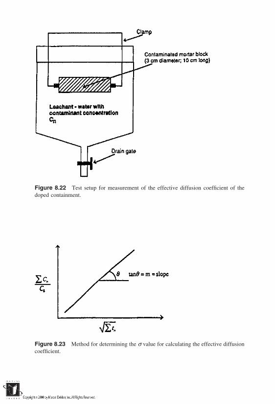
Figure 8.22 Test setup for measurement of the effective diffusion coefficient of thedoped containment.

Figure 8.23 Method for determining the σ value for calculating the effective diffusioncoefficient.

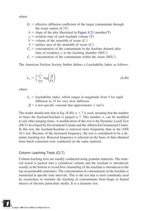
where

De effective diffusion coefficient of the target contaminant throughthe waste matrix (L2/T)

b slope of the plot illustrated in Figure 8.23 (number/T)tn resident time of each leachant volume (T)V volume of the monolith of waste (L3)S surface area of the monolith of waste (L2)

Cn concentration of the contaminant in the leachate drained aftertime of residence tn in the leaching chamber (M/L3)

Co concentration of the contaminant within the waste (M/L3)

The American Nuclear Society further defines a Leachability Index as follows:

Lw 17

7

n1

log βDe (8.40)

where

Lw leachability index, which ranges in magnitude from 5 for rapiddiffusion to 15 for very slow diffusion

β a test-specific constant that approximates 1 cm2/s

The reader should note that in Eq. (8.40), n 7 is used, meaning that the numberof times the leachant/leachate is purged is 7. This number, n, can be modifiedto suit other purging times. A modification of this test is the Dynamic Leach Test(DLT) developed by Environment Canada and the Alberta Environmental Center.In this test, the leachant/leachate is renewed more frequently than in the ANS16.1 test. Because of the increased frequency, the test is considered to be a dy-namic leaching test. Renewal frequency is selected on the basis of data obtainedfrom batch extraction tests conducted on the same material.

Column Leaching Tests (CLT)

Column leaching tests are usually conducted using granular materials. The mate-rial tested is packed into a cylindrical column and the leachant is introduced,usually at the bottom to avoid flow channeling (if the leachant is introduced at thetop on permeable materials). The concentration of contaminants in the leachate ismonitored at specific time intervals. This is the test that is most commonly usedby researchers to simulate the leaching of contaminants from heaps or buriedmasses of discrete particulate media. It is a dynamic test.

8.9.4 Theoretical Analysis of Contaminant Leaching Rates

From a theoretical standpoint, two types of leaching can be identified based onthe stabilized waste form:

1. Leaching of discrete particulate media2. Leaching of monoliths of waste

For particulate media leaching, percolation leaching equations have been pre-sented in Chapter 6. In addition, the release of substances from individualparticles of the medium can be further analyzed using particle size reduction–leaching time functions such as those applied in the ‘‘shrinking core model.’’The model is described in standard mineral processing textbooks and is not pre-sented here.

For monoliths, the release of the target contaminant into an adjacentleachant external to the monolith from locations x in the monolith measuredfrom the monolith-leachant boundary can be described using the following formof the one-dimensional advection-dispersion equation:

De∂2C

∂x2 Vv∂C

∂x 1 1 f

f ρtKd ∂C

∂x 0 (8.41)

where

De as defined for Eq. 8.39C concentration of the contaminant in the waste (M/L3)x distance from the waste/leachant boundary into the waste

monolith (L)Vv advective flow velocity of the contaminant from the monolith

to the leachant (L/T)f porosity of the matrix (dimensionless fraction)

ρt density of the matrix (M/L3)Kd distribution coefficient of the contaminant for the matrix solid

matter–pore fluid combination (L3/M)t time (T)

Other versions of Eq. (8.41) may contain moisture content terms, put in toreplace porosity terms. Furthermore, the tightness of pores in stabilized materials,which implies that both porosity and permeability magnitudes are very low,makes advective flow negligible. The primary mechanism for contaminant re-moval from the stabilized mass is then diffusion. Thus,

∂C

∂t De∂2C

∂x2 (8.42)

Equation (8.42) is commonly known as Fick’s second law of diffusion. Followingthe analytical solution developed by Crank (1975) and with the simplifying as-sumption that De will remain constant as leaching (and hence time) increases,Eq. (8.43) results for use in estimating the quantity of contaminant leached froma monolith.

Mt 2(C0 Ci) Det

π 0.5

(8.43)

where

Mt amount of contaminant leached per unit surface area of amonolith after a given time interval (M/L2)

Co initial concentration of the contaminant in the pore solution ofthe monolith (M/L3)

Ci concentration of the contaminant at the monolith/leachantinterface (M/L3)

Other parameters are as defined earlier.The concentration Ci can be assumed to be the same as the concentration

of the contaminant in the leachant/leachate. In reality, Ci is greater than the bulkleachant/leachate concentration of the target contaminant. Equilibration can beattained through mixing or through other forms of agitation of the reaction cham-ber. When the leachant is renewed, Ci is initially zero in magnitude.

Within the monolith itself, the contaminant partitions between the matrixand the liquid in the pore spaces. A partition coefficient or mass transfer coeffi-cient can be used to describe this partition. Hence,

C0 KpCd (8.44)

C0 Kpmd

vd (8.45)

where

Kp mass transfer (or partition coefficient) of the target contaminantbetween the pore solution and the matrix (dimensionlessfraction)

Cd mix design concentration of the contaminant per bulk volumeof the stabilized mass (M/L3)

md mass of the contaminant in the stabilized material (M)vd design volume of the stabilized material containing Md(L3)

If Kp is assumed to have its maximum possible value of 1.0 (the target contami-nant gets completely into the pore fluid) and Ci 0, then Eq. (8.44) can beintroduced into Eq. (8.43) resulting in the following equation:

Mt 2md

vdDet

π 0.5

(8.46)

Considering that Mt is expressed on a per-unit-surface-area basis, it needs to bemultiplied by the total external surface area of the monolith as follows, to obtainthe total quantity removed from the monolith:

MtT (Mt)(S) 2Smd

vdDet

π 0.5

(8.47)

where

MtT mass of the contaminant that leaches through the entireexternal surface of the monolith during a given time interval(M)

S total external surface area of the monolith (L2)

Equation (8.47) can then be rearranged as follows, noting that to use Eq. (8.48),vd must be the volume of the monolith that has the total surface area S.

MtT

md

2S

vdDet

π 0.5

(8.48)

Essentially, Eq. (8.48) is an expression for estimating the quantity of the contami-nant that can be removed from a monolith after a given duration of leachingexpressed as a fraction of the quantity that was originally put into the material.

8.10 EX-SITU CHEMICAL TREATMENT PRINCIPLES

Chemical treatment is the destruction or transformation of contaminants fromhazardous to less hazardous forms through direct or catalyzed chemical reactions.Catalysis reactions are more effective in the aqueous phase. Consequently, lowtreatment efficiencies are usually obtained for contaminants that are stronglysorbed to solid matrix components in soils. Secondly, the chemical reactions thatare necessary for decontamination involve stoichiometric combinations of thereactants, in the presence of impurities (soil particles) which interfere with, andinfluence, the effectiveness of the reactions. Most chemical treatment processeswere developed for treatment of aqueous streams of contaminants. Contact be-

tween reactants is more efficient in such streams than in contaminated soils.Therefore, chemical treatment of soil media that have high solids concentrationsmay require slurrying and aggressive mixing to produce adequate decontamina-tion levels. Difficulties associated with delivery of reactants to contaminated ma-terials in situ in proportions that satisfy stoichiometric requirements, control ofreaction conditions, and mixing, constrain chemical treatment to being primarilyan ex situ treatment process. However, recent developments have involved deepsoil mixing (with the reaction agents) and/or installation of subsurface walls ofreaction agents such as iron filings and limestone through which contaminatedwater can pass through to attain treatment. The most common chemical treatmentmethods are pH adjustment, oxidation/reduction, dehalogenation, hydrolysis, andsupercritical water oxidation. The principles that underlie these techniques arediscussed in this section. The reader should note that dehalogenation has beendiscussed in section 8.8.

8.10.1 Chemical Oxidation–Reduction Principles

Both chemical oxidation and reduction occur in the same process for differentreactants. Usually, the oxidation state of one compound is increased (the oxidizedcompound) while it is decreased for another compound (the reduced compound).The oxygen supplier is called the oxidizing agent, and the compound that acceptsoxygen is called the reducing agent. Chemical oxidation can also be defined asthe loss of electrons by the oxidized compound, while reduction is the gain ofelectrons by the reduced compound.

The most common classes of contaminants treated using oxidation are phe-nols, chlorophenols, cyanides, some pesticides, and halogenated aliphatics. Theprocess can be used in treating slurried contaminated soils that contain oxidizablecontaminants. Oxidation rates can be improved through the use of catalysts, radia-tion, and electrolytic treatment. Some of the most commonly used oxidizingagents are discussed briefly below.

Hydrogen Peroxide (H2O2)

Hydrogen peroxide is a colorless, weakly acidic liquid. The reactions throughwhich hydrogen peroxide can oxidize waste can be described as follows.

H2O2 R RO H2O (8.49)

Catalysts such as Fe3 and Fe2 can cause the decomposition of H2 O2 to radicalsof perhydroxyl and hydroxyl, which are very effective oxidants.

Fe2 H2O2 Fe2 OH OH (8.50)

Fe3 H2O2 Fe2 H HO2 (8.51)

The perhydroxyl and hydroxyl are HO2 and OH, respectively. A number of oxida-tion reactions referred to as ‘‘Fenton’s reactions’’ (Dorfman and Adams, 1973)can be induced through the use of these two oxidants. In high concentrations,some organics and inorganics may produce heat in reactions with H2O2.

Ozone (O3)

Ozone is a blue, excessively reactive gas which is capable of oxidizing a widevariety of compounds. When introduced into aqueous solutions that contain im-purities such as soil particles and contaminants, ozone decomposes quickly indirect proportion to the content of impurities in the water. Masschelein (1982)identifies the following pathways for the oxidation of organic compounds byozone, each of which results in different reaction products.

1. Direct oxidation2. Oxidation by hydroxyl formed by the decomposition of ozone in water3. Oxidation that results from ozone–solute interactions

The U.S. EPA (1986a) estimates that some compounds that have low reactionrates with ozone will react 100–1000 times faster if ultraviolet radiation or ultra-sonic energy is applied. High pH favors an increase in the reactions that involvethe hydroxyl free radical, which are normally slower than other reactions underlower pH conditions. Table 18.17 shows data on the ozonation of various organiccompounds in water.

Hypochlorites

Hypochlorites are formed by the reaction of chlorine with an alkali. Hyprochlor-ites such as calcium hypochlorites (CaOCl2) and sodium hypochlorite (NaOCl)are strong oxidizing agents and are used primarily as a safe method of deliveringchlorine. The addition of chlorine to contaminated media causes reactions thatfall into three classes of mechanisms:

1. Addition of chloride ion to the molecular structure of the compound2. Replacement of molecular units of the compound by chlorine3. Oxidation of the compound by chlorine

The first two mechanisms are generally called chlorination. If organic compoundsare the target contaminants, chlorinated organic compounds, which are generallytoxic, may be formed under suitable reaction conditions. This is common instrong solutions at low pH. Oxidation is favored in slightly acidic solutions and isthe desirable reaction in use of hypochlorites for treatment of organic compounds.

Reduction is also a viable technique for decontamination of polluted soilmedia. Examples of reducing agents are compounds of iron (as previously dis-cussed), zinc, sodium, and aluminum. Waste streams containing chromium, mer-

Table 8.17 Data on the Ozonation of Some Organic Compounds in Water

Initial Finalconc. Ozone dose Conc. Percent

Compound(s) (mg/liter) (mg/liter) (mg/liter) reduction

Methanol 2000 — 160 92Ethanol 1000 — 90 91Isoamyl alcohol 1000 — 80 92Glycerine 1000 — 0 100Hydrazine 100 — 0 100Carbon Disulfide 100 — 0 100Hydrogen Sulfide 10 — 0 100Phenol 100 — 0 100o-Cresol 100 — 0 100Hydroquinone 100 — 0 100Salicyclic acid 100 — 0 100Gasoline 1000 — 0 100Benzene 500 — 0 100Toluene 500 — 0 100Xylene 500 — 0 100Acetone 100 — 30 70Petroleum 10 4.5 0.2–0.3 97–98Gasoline 50 1.29 1 98

5.1 0.1 99.8Benzene 200 20 5 97.5Diethylbenzene 125–100 150–10 5–12.5 88–962,2,4-dinitrophenol 50 100 0.35 99.3

3 17 0.05 98.314 0 100

DDT 0.5 13.8 0.25 50Malathion 10 3.5 2 80

9.8 1 902.6 0 100

Methylparathion 10 4.5 0.5 959.5 0.1 99

Trichloromethyl 10 8–10 0.07 99.3parathion

0.5–1 3.5–4.5 0 100Dinitro- 10 5–6 0 100

orthocresol

Source: U.S. EPA (1986).

cury, chlorinated organics, and unsaturated organics can be treated by the reduc-tion method. For example, hexavalent chromium can be reduced to the less toxicand readily precipitable trivalent chromium. Both redox and oxidative treatmentprocesses often require a subsequent process for removal of reaction products.

8.10.2 Supercritical Water Oxidation

At temperatures and pressures near its critical point, the characteristics of watermake it an excellent medium for oxidation of compounds. At the critical pointof water, which is 374°C and 221 atm, hydrogen bonds of the water assume thecharacteristics of a polar solvent. At this stage, oxygen and almost all hydrocar-bons become readily soluble in water while the solubility of inorganic compoundsbecomes negligible. This implies that organic compounds can be oxidized whileinorganics can be precipitated by supercritical water.

The process described by the U.S. EPA (1987) involves mixing of aqueoussolutions or slurries of the target contaminated media with oxygen at pressuresgreater than 218 atm and temperatures in the regime of 500°C. This is accom-plished in either an above-ground pressure vessel or a buried reactor vessel. Thistreatment technique requires high energy input. Emissions and residues includegases (N2 and CO2), inorganic precipitates, and aqueous solutions of organicsand some salts. Oxidation and precipitation rates are typically very high.

8.10.3 Hydrolysis Principles

Hydrolysis is a complexation reaction in which hydroxyl (OH) liquid substitutesfor a detached group in a molecule such that the compound becomes more stable.Water is usually the source of the (OH) liquid, and the displacement reactioncan be represented as follows:

RX H2O ROH HX (8.52)

where R is the organic moiety and X is the chemical group that is cleaved offin the reaction. Even under natural conditions, hydrolysis of chemical compoundsdoes occur. For decontamination of soils, the purpose is to induce environmentalconditions that can increase its rate of occurrence. Organic compounds hydrolyzenaturally in rates that range from a few seconds to millions of years. The ratesare generally of first-order or pseudo-first-order form. The organic compoundsthat are susceptible to hydrolysis are listed below with representative reactionequations using information mostly adapted from U.S. EPA (1986).

Alkyl halides: RX H2O ROH HX (8.53)

Esters: R1C(O)OR2 H2O R1C(O)OH R2OH (8.54)

Amides: RC(O)NR1R2 H2O RC(O)OH R1R2NH (8.55)

Carbamates: ROC(O)NR1R2 H2OROHHNR1R2 CO2 (8.56)

Phosphoric and phosphoric acid esters:

ROPR1R2 H2O HOPR1R2 ROH (8.57)

As in the previous reaction equation, R represents the organic moiety, which maybe of one type in the parent organic compound. In some cases some moietieswithin the same compound can be hydrolyzable while others may not be hydro-lyzable. Also, the hydrolysis of various moities or part of the compound may becontingent upon different conditions of pH, temperature, etc.

Generally, the hydrolysis rate of a compound is regarded as the sum ofneutral, acid-catalyzed, and base-catalyzed process constants, as follows:

∂(RX)

∂t kN(RX) kA(RX)(H) kB(RX)(OH) (8.58)

where

RX the concentration of the organic contaminantt time

kN neutral hydrolysis reaction constant (for pH7.0)kA acid-catalyzed hydrolysis reaction constant (for pH 7.0)kB base-catalyzed hydrolysis reaction constant (for pH 7.0)

kh kN kA(H) kB(OH) (8.59)

In Eq. (8.59), kh is the overall hydrolysis reaction rate constant. Equation (8.58)can then be rewritten as Eq. 8.60:

∂(RX)

∂t kh(RX) (8.60)

The U.S. EPA (1986) has compiled data on hydrolysis rates of various organiccompounds. These data are presented in Tables 8.18–8.21. The reader shouldnote that these hydrolysis rates are at temperatures at or near 25°C. Applicationof hydrolysis as a treatment technique to contaminated media to achieve rateshigher than those at normal temperature and pH conditions may require alterationof these conditions. Generally, hydrolysis intensifies with increase in temperature.Information provided on pH dependence tabulated in Tables 8.18–8.21 can alsobe used to increase rates.

Table 8.18 Data on the Hydrolysis of Halogenated Ethers, Epoxides, and Alcohols

t1/2 at pHData

Compound source kA kN kB 5 6 7 8 9 10 11

Chloromethylmethylether 1 — — — — — 0.007s — — — —bia(Chloromethyl)ether 1 — — — — — 38s — — — —2-Chloroethanol 1 — — — — — 21y — — — —1-Chloro-2-propanol 1 — — — — — 2 y — — — —2-Chloroethylvinylether 2 — — — — — 0.48 y — — — —3-Chloro-,1,2 epoxy, 2-methyl propane 3 1.84E-3 5E-7 — 16d 16d 16d 16d 16d 16d 16dAlpha-epichlorohydria 3 8.0E-4 9.8E-7 — 8.2d 8.2d 8.2d 8.2d 8.2d 8.2d 8.2dEpibromohydrin 3 6.1E-4 5E-7 — 16d 16d 16d 16d 16d 16d 16d

Note: All values reported for 25°C. Rate constants in s1; a second; d day; y year.Data sources: 1. Radding et al. (1977); 2. Versar, Inc. 1979; 3. Mabey and Mill (1978).Source: U.S. EPA (1986).

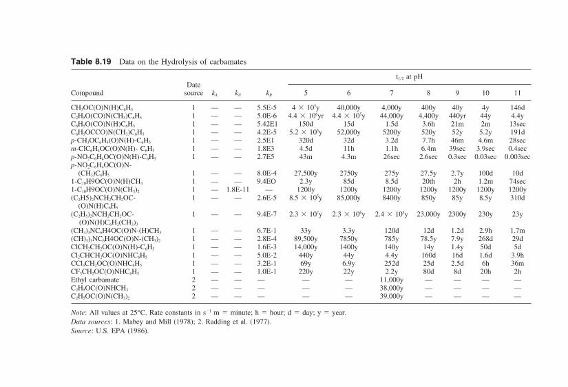
Table 8.19 Data on the Hydrolysis of carbamates

t1/2 at pHDate

Compound source kA kN kB 5 6 7 8 9 10 11

CH3OC(O)N(H)C6H5 1 — — 5.5E-5 4 105y 40,000y 4,000y 400y 40y 4y 146dC2H5O(CO)N(CH3)C6H5 1 — — 5.0E-6 4.4 106yr 4.4 105y 44,000y 4,400y 440yr 44y 4.4yC6H5O(CO)N(H)C6H5 1 — — 5.42E1 150d 15d 1.5d 3.6h 21m 2m 13secC6H5OCCO)N(CH3)C6H5 1 — — 4.2E-5 5.2 105y 52,000y 5200y 520y 52y 5.2y 191dp-CH3OC6H4(O)N(H)-C6H5 1 — — 2.5E1 320d 32d 3.2d 7.7h 46m 4.6m 28secm-ClC6H4OC(O)N(H)- C6H5 1 — — 1.8E3 4.5d 11h 1.1h 6.4m 39sec 3.9sec 0.4secp-NO2C6H4OC(O)N(H)-C6H5 1 — — 2.7E5 43m 4.3m 26sec 2.6sec 0.3sec 0.03sec 0.003secp-NO2C6H4OC(O)N-

(CH3)C6H5 1 — — 8.0E-4 27,500y 2750y 275y 27.5y 2.7y 100d 10d1-C10H9OC(O)N(H)CH3 1 — — 9.4EO 2.3y 85d 8.5d 20th 2h 1.2m 74sec1-C10H9OC(O)N(CH3)2 1 — 1.8E-11 — 1200y 1200y 1200y 1200y 1200y 1200y 1200y(C2H5)2NCH2CH2OC- 1 — — 2.6E-5 8.5 105y 85,000y 8400y 850y 85y 8.5y 310d

(O)N(H)C6H5

(C2H5)2NCH2CH2OC- 1 — — 9.4E-7 2.3 107y 2.3 106y 2.4 105y 23,000y 2300y 230y 23y(O)N(H)C6H3(CH3)3

(CH3)3NC6H4OC(O)N-(H)CH3 1 — — 6.7E-1 33y 3.3y 120d 12d 1.2d 2.9h 1.7m(CH)3)3NC6H4OC(O)N-(CH3)2 1 — — 2.8E-4 89,500y 7850y 785y 78.5y 7.9y 268d 29dClCH2CH2OC(O)N(H)-C6H5 1 — — 1.6E-3 14,000y 1400y 140y 14y 1.4y 50d 5dCl2CHCH2OC(O)NHC6H5 1 — — 5.0E-2 440y 44y 4.4y 160d 16d 1.6d 3.9hCCl3CH2OC(O)NHC6H5 1 — — 3.2E-1 69y 6.9y 252d 25d 2.5d 6h 36mCF3CH2OC(O)NHC6H5 1 — — 1.0E-1 220y 22y 2.2y 80d 8d 20h 2hEthyl carbamate 2 — — — — — 11,000y — — — —C2H5OC(O)NHCH3 2 — — — — — 38,000y — — — —C2H5OC(O)N(CH3)2 2 — — — — — 39,000y — — — —

Note: All values at 25°C. Rate constants in s1 m minute; h hour; d day; y year.Data sources: 1. Mabey and Mill (1978); 2. Radding et al. (1977).Source: U.S. EPA (1986).

8.11 IN-SITU NATURAL ATTENUATION PRINCIPLES

Natural attenuation, which is also called intrinsic or passive remediation, is atechnique in which natural processes in soil systems are relied upon to degradeand dissipate contaminants. Contaminant dissipation may occur through elimina-tion or transformation. If conditions in a soil system favor the occurrence ofnatural attenuation, the implication is that the necessity to clean up the soil systemto very low residual contaminant concentrations is minimized.

Soil systems contain natural materials such as microbes, aqueous iron, ironminerals, reduced sulfur, and soil organic matter. The interaction of these materi-als with contaminants can result in natural attenuation. The distinction betweennatural attenuation processes and associated processes that result in the transferof contaminants from the aqueous phase to the solid phase (sorption and precipita-tion) has been controversial. Both sets of processes are interrelated, but naturalattenuation implies a decrease in the concentrations of the target contaminantswithin the total soil system and not a transfer from one phase to another as inthe case of sorption. Both natural attenuation and phase-transfer processes resultin a decrease in contaminant concentration in the aqueous phase.

Figure 8.24 illustrates contaminant plume migration from a source that isinduced by groundwater movement through the source zone. The plume travelsat a velocity Vmin from the source zone. Natural attenuation occurs within theplume zone and will occur in the intervening zone between the plume and thepoint of compliance (POC). Undoubtedly, the concentration of contaminants thatwill be obtained through sample retrieval from the POC and analytical measure-ments is expected to be lower than those for preceding points in this box model.This will be true if the plume travels at a rate faster than the rate of contaminantreplenishment from the source. The reduction in contaminant concentration atthe POC relative to all preceding points (in this homogeneous, isotropic, andcontinuous geomedia model) is attributable to the following factors.

1. Sorption of contaminants by soil materials with which the contami-nants come in contact

2. Precipitation of contaminants along the path of travel if favored byprevailing groundwater chemistry and pH-Eh conditions

3. Destruction and transformation of contaminants by microbes and soilminerals

Natural attenuation is generally considered to be primarily factors 2 and3. The U.S. EPA (1995) conveniently describes natural attenuation processes oforganic contaminants as outlined in Table 8.22. For biological processes, aerobicbiodegradation rates are commonly higher than anaerobic rates. Typically, theplume that undergoes natural attenuation comprises an inner anaerobic core andan outer aerobic core as shown in Figure 8.25. Aerobic biodegradation of the

Table 8.20 Data on the Hydrolysis of Esters

t1/2 at pHData

Compound source kA kN kB 5 6 7 8 9 10 11

Ethyl acetate 1 1.1E-4 1.5E-10 1.1E-1 16y 16y 2.0y 0.2y 7.3d 0.73d 0.073dIsopropyl acetate 1 6.0E-5 — 2.6E-2 35y 68y 8.4y 308d 31d 3.1d 0.31dButyl acetate 1 1.3E-4 — 1.5E-3 1.6y 78y 140y 1.5y 015y 5.5d 0.5dVinyl acetate 1 1.4E-4 1.1E-7 1.0E1 73d 67d 7.3d 0.8d 1.9h 12m 1.2mAllyl acetate 1 — — 7.3E-1 30y 3.0y 110d 11d 1.1d 2.6h 0.26hBenzyl acetate 1 1.1E-4 — 2.0E-1 17y 10.4y 1.1y 40d 4.0d 9.6h 1hO-Acetyl phenol 1 7.8E-5 6.6E-8 1.4E0 119d 100d 38d 5.5d 0.57d 1h 5m2,4-Dinitrophenyl acetate 1 — 1.1E-5 9.4E1 17h 16h 9.4h 1.8h 0.2h 1.2m 1 1mClCH2C(O)0CH3 1 8.5E-5 2.1E-7 1.4E2 23d 5.0d 14h 1.4h 8.3m 50s 5sCl2CHC(O)OCH3 1 2.3E-4 1.5E-5 2.8E3 11h 4.5h 38m 4.1m 255 2.5s 0.2sCl2CHC(O)OC6H5 1 — 1.8E-3 1.3E4 6.4m 6.1m 3.7m 47s 4.7s 0.5s 0.05sF2CHC(O)OC2H5 1 — 5.7E-5 4.5E3 3.3h 1.9h 23m 2.6m 16s 1.6s 0.2sCl3CC(O)OCH3 1 — 7.7E-4 — 15m 15m 15m 15m 15m 15m 15mF3CC(O)OC2H5 1 — 3.2E-3 — 3.6m 3.6m 3.6m 3.6m 3.6m 3.6m 3.6mF3CC(O)OC(CH3)3 1 — 1.3E-3 — 8.9m 8.9m 8.9m 8.9m 8.9m 8.9m 8.9mCH3SCH2C(O)OC2H5 1 — — 9.2E-1 24y 2.4y 87d 8.7d 0.87d 2.1h 13mCH3S(O)CHC(O)C2H5 1 — — 1.3E1 1.7y 62d 6.2d 0.62d 1.5h 9m 1m

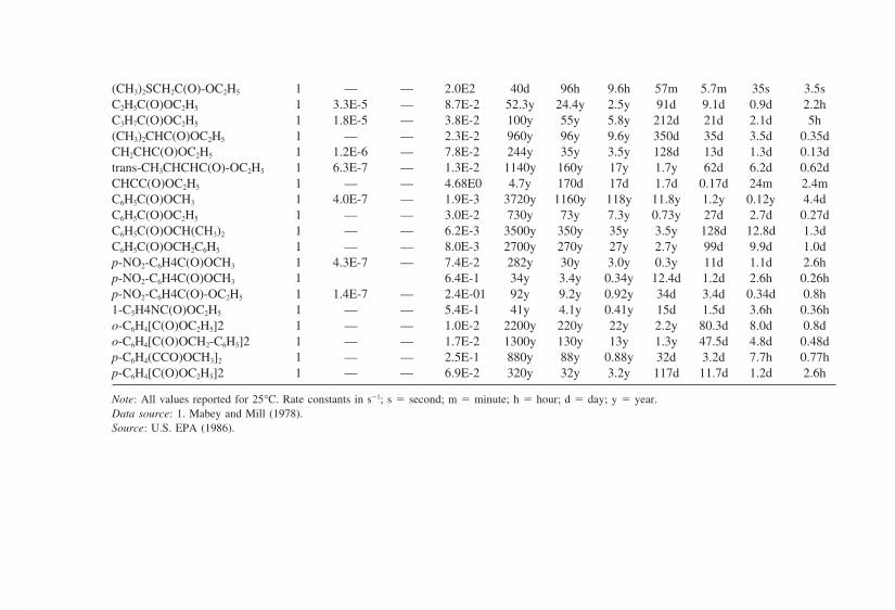
(CH3)2SCH2C(O)-OC2H5 1 — — 2.0E2 40d 96h 9.6h 57m 5.7m 35s 3.5sC2H5C(O)OC2H5 1 3.3E-5 — 8.7E-2 52.3y 24.4y 2.5y 91d 9.1d 0.9d 2.2hC3H7C(O)OC2H5 1 1.8E-5 — 3.8E-2 100y 55y 5.8y 212d 21d 2.1d 5h(CH3)2CHC(O)OC2H5 1 — — 2.3E-2 960y 96y 9.6y 350d 35d 3.5d 0.35dCH2CHC(O)OC2H5 1 1.2E-6 — 7.8E-2 244y 35y 3.5y 128d 13d 1.3d 0.13dtrans-CH3CHCHC(O)-OC2H5 1 6.3E-7 — 1.3E-2 1140y 160y 17y 1.7y 62d 6.2d 0.62dCHCC(O)OC2H5 1 — — 4.68E0 4.7y 170d 17d 1.7d 0.17d 24m 2.4mC6H5C(O)OCH3 1 4.0E-7 — 1.9E-3 3720y 1160y 118y 11.8y 1.2y 0.12y 4.4dC6H5C(O)OC2H5 1 — — 3.0E-2 730y 73y 7.3y 0.73y 27d 2.7d 0.27dC6H5C(O)OCH(CH3)2 1 — — 6.2E-3 3500y 350y 35y 3.5y 128d 12.8d 1.3dC6H5C(O)OCH2C6H5 1 — — 8.0E-3 2700y 270y 27y 2.7y 99d 9.9d 1.0dp-NO2-C6H4C(O)OCH3 1 4.3E-7 — 7.4E-2 282y 30y 3.0y 0.3y 11d 1.1d 2.6hp-NO2-C6H4C(O)OCH3 1 6.4E-1 34y 3.4y 0.34y 12.4d 1.2d 2.6h 0.26hp-NO2-C6H4C(O)-OC2H5 1 1.4E-7 — 2.4E-01 92y 9.2y 0.92y 34d 3.4d 0.34d 0.8h1-C5H4NC(O)OC2H5 1 — — 5.4E-1 41y 4.1y 0.41y 15d 1.5d 3.6h 0.36ho-C6H4[C(O)OC2H5]2 1 — — 1.0E-2 2200y 220y 22y 2.2y 80.3d 8.0d 0.8do-C6H4[C(O)OCH2-C6H5]2 1 — — 1.7E-2 1300y 130y 13y 1.3y 47.5d 4.8d 0.48dp-C6H4(CCO)OCH3]2 1 — — 2.5E-1 880y 88y 0.88y 32d 3.2d 7.7h 0.77hp-C6H4[C(O)OC2H5]2 1 — — 6.9E-2 320y 32y 3.2y 117d 11.7d 1.2d 2.6h

Note: All values reported for 25°C. Rate constants in s1; s second; m minute; h hour; d day; y year.Data source: 1. Mabey and Mill (1978).Source: U.S. EPA (1986).

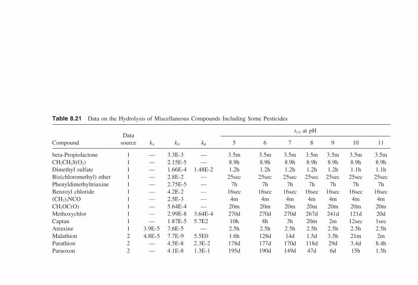
Table 8.21 Data on the Hydrolysis of Miscellaneous Compounds Including Some Pesticides

t1/2 at pHData

Compound source kA kN kB 5 6 7 8 9 10 11

beta-Propiolactone 1 — 3.3E-3 — 3.5m 3.5m 3.5m 3.5m 3.5m 3.5m 3.5mCH2CH2S(O2) 1 — 2.15E-5 — 8.9h 8.9h 8.9h 8.9h 8.9h 8.9h 8.9hDimethyl sulfate 1 — 1.66E-4 1.48E-2 1.2h 1.2h 1.2h 1.2h 1.2h 1.1h 1.1hBis(chloromethyl) ether 1 — 2.8E-2 — 25sec 25sec 25sec 25sec 25sec 25sec 25secPhenyldimethyltriaxine 1 — 2.75E-5 — 7h 7h 7h 7h 7h 7h 7hBenzoyl chloride 1 — 4.2E-2 — 16sec 16sec 16sec 16sec 16sec 16sec 16sec(CH3)2NCO 1 — 2.5E-3 — 4m 4m 4m 4m 4m 4m 4mCH3OC(O) 1 — 5.64E-4 — 20m 20m 20m 20m 20m 20m 20mMethoxychlor 1 — 2.99E-8 3.64E-4 270d 270d 270d 267d 241d 121d 20dCaptan 1 — 1.87E-5 5.7E2 10h 8h 3h 20m 2m 12sec 1secAtraxine 1 3.9E-5 7.6E-5 — 2.5h 2.5h 2.5h 2.5h 2.5h 2.5h 2.5hMalathion 2 4.8E-5 7.7E-9 5.5E0 1.6h 128d 14d 1.5d 3.5h 21m 2mParathion 2 — 4.5E-8 2.3E-2 178d 177d 170d 118d 29d 3.4d 8.4hParaoxon 2 — 4.1E-8 1.3E-1 195d 190d 149d 47d 6d 15h 1.5h

Diazinon 2 2.1E-2 4.3E-8 5.3E-3 32d 125d 176d 165d 14d 14d 1.5dDiazoxon 2 6.4E-1 2.8E-7 7.6E-6 1.2d 9d 23d 28d 29d 29d 29dChlopyrifos 2 — 1.E-7 1E-1 80d 79d 73d 40d 7d 19h 2hSevin 2 — — 7.7E0 2.9h 104d 10d 1d 2.5h 15m 1.5mSevin 2 — — 3.4E0 6.5y 236d 24d 2.4d 5.7h 34m 3.4mBaygon 2 — — 4.6E-1 48y 4.8y 174d 17d 1.7d 4.2h 25mPyrolam 2 — — 1.1E-2 2000y 200y 20y 2y 73d 7.3d 18hDimetilan 2 — — 5.7E-5 3.9 105y 39,000y 3900y 390y 39y 3.9y 141dP-Nitrophenyl-N-methyl 2 — 4E-5 3.0E3

carbamate 4.5h 2.8h 34m 3.8m 23sec 2.3sec 0.23sec2,4-D,m- 2 2.0E-5 2.0E-5 3.02E1butoxyethylester 9.6h 9.5h 8.4h 4.4h 36m 4m 23secMethoxychlor 2 — 2.8E-8 2.8E-4 286d 286d 286d 286d 252d 122d 20dDDT 2 — 1.9E-9 9.9E-3 12y 11y 7.6y 1.9y 79d 8d 19h2,4-D,methylester 2 — — 1.7E1 1.3yr 47d 4.7d 11hr 1.1hr 6.8min 41sec

Note: All values for 25 5°C. Rate constants in s1; m minute; h hour; d day; y year.Data sources: 1. Mabey and Hill (1978); 2. Harris (1982).Source: U.S. EPA (1986).

Figure 8.24 Illustration of contaminant plume movement within a box model: Vw groundwater velocity through the contaminant (of mass M0) source zone; Vmin plumevelocity. (Adapted from U.S. EPA, 1994b.)

outer core is enhanced by its greater access to infiltrating oxygen than the innercore. From the analysis developed by Kerfoot (1994), the oxidation of a hydrocar-bon (an organic compound class) can be described as follows:

CxHy (x y)4 O2 xCO2 y

2H2O (8.61)

CxHy is the empirical formula of this generic hydrocarbon. Considering that car-bon has an atomic mass of 12 amu and hydrogen has an atomic mass of 1 amu,each mole of CxHy has a mass of (12x y) gram, and is degraded by [x (y/4)] moles or (32x 8y) gram of molecular oxygen to produce 1 mole or (44x)gram of CO2.

For hydrocarbons with the following x and y values, Kerfoot (1994) pro-vides the approximations indicated below for rates of oxygen consumption, hy-drocarbon degradation, and CO2 production.

For x y 2x and 4x12:

∂(CxHy)∂(O2)

0.31 (8.62)

∂(CxHy)∂(CO2)

0.31 (8.63)

Inorganic contaminants such as metals can also be naturally attenuated insoil systems. Electron donors such as Fe2, ferrous iron minerals, organic matter,and reduced sulfur, which are present in soils in various proportions, can reduce

Table 8.22 The Most Prevalent Natural Attenuation Mechanisms

Potential For BTEXMechanism Description attenuation

BiologicalAerobic Microbes utilize oxygen as an Most significant attenuation

electron acceptor to convert mechanism if sufficient oxy-contaminant to CO2, water, gen is present. Soil air (O2)and biomass. 2%. Groundwater D.O.

1–2 mg/liter.Anaerobic Alternative electron acceptors Rates are typically much

Denitrification (e.g., NO3, SO4

2, Fe3, slower than for aerobic bio-Sulfate-reducing CO2) are utilized by mi- degradation: toluene is theMethanogenic crobes to degrade contami- only component of BTEXFe-reducing nants. that has been shown to con-

sistently degrade.Hypoxic Secondary electron acceptor re- Has not been demonstrated in

quired at low oxygen con- the field for BTEX.tent for biodegradation ofcontaminants.

PhysicalVolatilization Contaminants are removed Normally minor contribution

from groundwater by volatil- relative to biodegradation.ization to the vapor phase More significant for shallowin the unsaturated zone. or highly fluctuating water

table.Dispersion Mechanical mixing and molec- Decreases concentrations, but

ular diffusion processes re- does not result in a net lossduce concetrations. of mass.

Sorption Contaminants partition be- Sorption retards plume migra-tween the aqueous phase tion, but does not perma-and the soil matrix. Sorp- nently remove BTEX fromtion is controlled by the or- soil or groundwater as de-ganic carbon content of the sorption may occur.soil, soil mineralogy, andgrain size.

Source: U.S. EPA (1995).

contaminants such as Cr(VI). The reaction equation for the reduction of Cr(VI)by Fe2 is as follows:

3Fe2 HCrO4 7H Cr3 3Fe3 4H2O (8.64)

Eary and Rai (1988) estimate that if sufficient dissolved oxygen gains access tothe reactants, the reaction may reach completion in less than 5 min.

Figure 8.25 Illustration of the effects of oxygen access on biodegradation of a contami-nant plume (U.S. EPA, 1995).

Many rock-forming minerals which are subsequently weathered to soilminerals contain iron. Among these minerals are olivines, micas, smectites, andpyroxenes. Iron-based minerals such as ilmenite, magnetite, and pyrite are com-mon soil minerals that may reduce oxidants such as hexavalent chromium.

Organic matter is also known to reduce metallic radicals such as chromates.An example of this reaction is presented below.

2Cr2O72 3C0 16H 4Cr3 3CO2 8H2O (8.65)

In summary, natural attenuation is adequate only when contaminant con-centrations are low enough to be dissipated by natural processes in soils. Exces-sive concentration of contaminants requires the application of active remediationtechniques.

8.12 IN-SITU PHYTOREMEDIATION PRINCIPLES

Phytoremediation is the use of plants to remove contaminants from soil systems,either in situ or in batch reaction systems. In-situ phytoremediation involves thedirect removal or transformation of contaminants in soil systems by growingplants, and is the focus of this section. This technique can be used to remediatesoil systems contaminated with metals, chlorinated solvents, crude oil, pesticides,and explosives such as trinitrotoluene (TNT).

In phytoremediation, one or a combination of plants is selected and culti-vated on a contaminated site. During their growth, the buried portions (roots)remove contaminants from soils through one or more of the following processes:direct absorption; transformation by microbes in the root zone; and stabilizationthrough phase-change processes (example: precipitation) and reduction of soilpermeability. Fractions of the mass of the contaminants that are absorbed by theroots of the plants are translocated to other parts (stem and leaves) of the plantsand accumulate for use in metabolic processes. Some of the absorbed contami-nants are volatilized, mostly through leaves into the atmosphere. The accumulatedcontaminants can be harvested along with the host plants and processed for dis-posal in reduced volume or for recycling.

Phytoremediation is useful at sites where targeted contaminants exist pri-marily within the depth of the root zone in concentrations that are low to moder-ate. Considering that reliance is on plant growth and efficient interaction withsoil contaminants, only plants that can tolerate the soil environmental conditions,including contamination levels and micro and macroclimates, can be used effec-tively. Such plants must also have adequately rapid growth rates and root densi-ties that are high enough to provide adequate surface area for contact with con-taminated soil media. Most plants that show high potential as phytoremediatorsgrow in tropical areas such as sub-Saharan Africa, Central and South America,

and the Caribbean Islands. Moffat (1995) explains that contaminant accumulationin these plants is a natural defense against plant-eating insects and microbialpathogens that abound in the tropics. The different techniques applied in in-situphytoremediation are described briefly below.

8.12.1 Phytoextraction

Phytoextraction is also referred to as phytoaccumulation. It is the uptake of con-taminants (usually metals) by plants and subsequent distribution of the contami-nants to plant stems and leaves, which can be harvested for concentration andrecycling or disposal of the metals. The harvested plant is usually composted orincinerated. Incineration to ash reduces the volume of the material to only about10% of the original. The contaminated site can be replanted with the selectedplants until contaminant concentrations in surficial soils are reduced to desiredlevels. Plants which have high capacities to accumulate metals are called hyperac-cumulators. Examples are presented in Table 8.23 and illustrated for nickel up-take in Figure 8.26.

Hundreds of plants in various locations around the world are known toabsorb high quantities of metals such as zinc, copper, and nickel. The U.S. EPA(1996b) recognizes hyperaccumulation as an ecophysiological adaptation ofplants to stress and as an indicator of resistance to metals that are usually foundwhere such hyperaccumulators thrive. Baker and Brooks (1989) define a hyperac-cumulator as a plant that contains more that 0.1% Ni, Co, Cu, or Cr, or 1.0%Zn and Mn, in its leaves on a dry-weight basis. Lack of sufficient biomass in

Table 8.23 Examples of Hyperaccumulators of Metals

Percentage ofMetal in Dry

Metal Plant species Weight of Leaves (%) Native Location

Zn Thlaspi calaminare 3 GermanyViola species 1 Europe

Cu Aeolanthus biformifolius 1 ZaireNi Phyllanthus serpentinus 3.8 New Caledonia

Alyssum bertoloni and 50 3 Southern Europe andother species of Alyssum Turkey

Sebertia acuminata 25 (in latex) New CaledoniaStackhousia tryonii 4.1 Australia

Pb Brassuca juncea 3.5 IndiaCo Haumaniastrum robertii 1 Zaire

Source: U.S. EPA, 1996b.

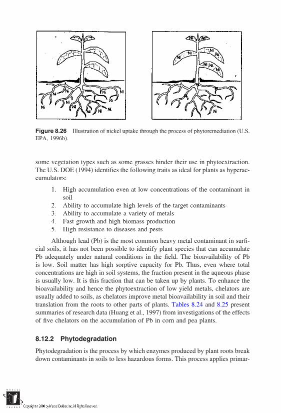
Figure 8.26 Illustration of nickel uptake through the process of phytoremediation (U.S.EPA, 1996b).

some vegetation types such as some grasses hinder their use in phytoextraction.The U.S. DOE (1994) identifies the following traits as ideal for plants as hyperac-cumulators:

1. High accumulation even at low concentrations of the contaminant insoil

2. Ability to accumulate high levels of the target contaminants3. Ability to accumulate a variety of metals4. Fast growth and high biomass production5. High resistance to diseases and pests

Although lead (Pb) is the most common heavy metal contaminant in surfi-cial soils, it has not been possible to identify plant species that can accumulatePb adequately under natural conditions in the field. The bioavailability of Pbis low. Soil matter has high sorptive capacity for Pb. Thus, even where totalconcentrations are high in soil systems, the fraction present in the aqueous phaseis usually low. It is this fraction that can be taken up by plants. To enhance thebioavailability and hence the phytoextraction of low yield metals, chelators areusually added to soils, as chelators improve metal bioavailability in soil and theirtranslation from the roots to other parts of plants. Tables 8.24 and 8.25 presentsummaries of research data (Huang et al., 1997) from investigations of the effectsof five chelators on the accumulation of Pb in corn and pea plants.

8.12.2 Phytodegradation

Phytodegradation is the process by which enzymes produced by plant roots breakdown contaminants in soils to less hazardous forms. This process applies primar-

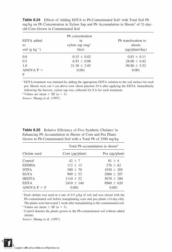
Table 8.24 Effects of Adding EDTA to Pb-Contaminated Soila with Total Soil Pbmg/kg on Pb Concentration in Xylem Sap and Pb Accumulation in Shootsb of 21-day-old Corn Grown in Contaminated Soil

Pb concentrationEDTA added in Pb translocation toto xylem sap (mg/ shootssoil (g kg1) liter) (µg/plant/day)

0.0 0.15 0.02 0.83 0.110.5 6.93 0.08 28.00 0.421.0 21.30 2.05 99.80 5.52ANOVA P 0.001 0.001F

a EDTA treatment was initiated by adding the appropriate EDTA solution to the soil surface for eachpot. Shoots were cut 1 cm above root–shoot junction 24 h after applying the EDTA. Immediatelyfollowing the harvest, xylem sap was collected for 8 h for each treatment.

b Values are mean SE (n 3).Source: Huang et al. (1997).

Table 8.25 Relative Efficiency of Five Synthetic Chelatesa inEnhancing Pb Accumulation in Shoots of Corn and Pea PlantsGrown in Pb-Contaminated Soil with a Total Pb of 2500 mg/kg

Total Pb accumulation in shootsb

Chelate used Corn (µg/plant) Pea (µg/plant)

Controlc 42 7 81 4EDDHA 112 13 276 62DTPA 300 70 1930 205EGTA 909 53 2080 207HEDTA 1110 52 5670 280EDTA 2410 140 8960 620ANOVA P F 0.001 0.001

a Each chelate was used at a rate of 0.5 g/kg of soil and was mixed with thePb-contaminated soil before transplanting corn and pea plants (14-day-old).The plants were harvested 1 week after transplanting to the contaminated soil.

b Values are mean SE (n 3).c Control denotes the plants grown in the Pb-contaminated soil without added

chelate.Source: Huang et al. (1997).

ily to organic compounds. The organic compounds are converted into simplermolecules which can be absorbed by the plant for growth. For example, poplartrees have been found (Newman et al., 1997) to be capable of taking up trichloro-ethylene (TCE) from contaminated soils and converting it inside the plants tometabolites such as trichloroethanol, trichloroacetic acid, and dichloracetic acid.Several plant enzymes, including nitroreductase, are also capable of breakingdown TNT (2,4,6-trinitrotoluene). In general, herbicides, chlorinated solvents,and ammunition wastes can be remediated by phytodegradation.

8.12.3 Rhizosphere Biodegradation

In rhizosphere biodegradation, microorganisms such as yeasts, fungi, and bacteriathat exist in the root zone degrade organic compounds present in soil. The com-pounds provide additional nutrients for the microbes to supplement the sugars,acids and alcohols secreted by plant roots.

8.12.4 Phytovolatilization

Phytovolatilization is the process by which plants are used to extract contami-nants from soils and release them to the atmosphere as gases. It is estimated (U.S.EPA, 1996b) that poplar trees volatilize about 90% of the TCE quantity, thatthey take up from soils. Metals can be produced in their volatile forms by meta-bolic activities in plants and volatilized into the atmosphere. For example, intro-duction of the bacterial gene called mercury reductase into some mustard plantscan reduce uptaken mercury to its gaseous form Hg(0), in which it can be volatil-ized by the plants.

8.12.5 Phytostabilization

Phytostabilization is the process by which plants immobilize contaminants insoils through sorption, complexation, precipitation, and changes in soil structure.Unlike most of the other phytoremediation processes, phytostabilization involvesprocesses that are external to the internal structure of the plants. In the DuPontphytostabilization process, soil amendments such as alkalizing agents, mineraloxides, organic matter, and biosolids are added to soils which are then plantedwith phytostabilizers. The fibrous roots of these plants hold the soil particlestogether and promote the processes mentioned above, thereby reducing the leach-ing potential of contaminants that are present in the soil.

8.13 IN-SITU BIOREMEDIATION PRINCIPLES

Bioremediation techniques are very diverse, and include landfarming, biorecla-mation, and even composting. However, the focus of this section is on biorecla-mation, which is herein defined as the addition of nutrients and oxygen to subsur-face contaminated media to enhance the biodegradation of contaminants bynaturally occurring microbes and/or microbes introduced into the subsurface.While some naturally occurring microorganisms are capable of degrading organiccompounds, others can be genetically engineered to target specific contaminantsfor degradation. Figure 8.27 shows the configuration of a bioreclamation systemin the field. The contaminant present in a soil mass in the vadose zone is flusheddown into groundwater using aerated water containing nutrients. This water isalso introduced upstream. The contaminants leached from the waste mass arebiodegraded in the plume especially at the aeration zone shown in the figure.Down gradient, the treated water is extracted for re-aeration, reinnoculation withnutrients/and possibly microbes, and recycling into the ground. Several factorsinfluence the effectiveness of in-situ bioreclamation systems. The process factorsare discussed briefly below.

8.13.1 Contaminant Intrinsic Biodegradability

It is believed that the intrinsic biodegradability of a chemical compound is sig-nificantly related to its chemical structure. Typically, laboratory measurementsare conducted to obtain data on surrogate parameters that reflect the effects ofchemical structure and form on biodegradation. A common parameter is the ratioof the 5-day biochemical oxygen demand (BOD5) to the chemical oxygen demand(COD). In general, the following designations are made:

BOD5

COD 0.01 biodegradable

BOD5

COD 0.01 nonbiodegradable

Another empirical measure of contaminant biodegradability is the refrac-tory index (RI), defined as the ratio of the ultimate biochemical oxygen demand(BODu) to the ultimate oxygen demand (UOD).

RI 0.5 generally biodegradableRI 0.5 generally nonbiodegradable

Figure 8.27 Schematic illustration of contaminated groundwater bioreclamation (U.S.EPA, 1986).

Tables 8.26 and 8.27 provide data on both the BOD5/COD ratios and RIof some contaminants. The reader should note that these classifications are some-what generic. Compounds with low ratios may still be biodegraded through useof specifically engineered microbes, provision of enough oxygen, and implemen-tation of other process optimization measures.

Waste masses usually contain a combination of biodegradable compounds,

Table 8.26 BOD5/COD Ratios for Various Organic Compoundsa

Compound Ratio Compound Ratio

Relatively Nondegradable p-Xylene 0.11Butane 0 Urea 0.11Butylene 0 Toluene 0.12Carbon tetrachloride 0 Potassium cyanide 0.12Chloroform 0 Isopropyl acetate 0.131,4-Dioxane 0 Amyl acetate 0.13–0.34Ethane 0 Chlorobenzene 0.15Heptane 0 Jet fuels (various) 0.15Hexane 0 Kerosene 0.15Isobutane 0 Range oil 0.15Isobutylene 0 Glycerine 0.16Liquefied natural gas 0 Adiponitrile 0.17Liquefied petroleum gas 0 Furfural 0.17–0.46Methane 0 2-Ethyl-3-propylacrolein 0.19Methyl bromide 0 Methylethylpyridine 0.20Methyl chloride 0 Vinyl acetate 0.20Monochlorodifluoromethane 0Nitrobenzene 0 Naphthalene (molten) 0.20Propane 0 Dibutyl phthalate 0.20Propylene 0 Hexanol 0.20Propylene oxide 0 Soybean oil 0.20Tetrachloroethylene 0 Paraformaldehyde 0.20Tetrahydronaphthalene 0 n-Propyl alcohol 0.20–0.63l-Pentene 0.002 Methyl methacrylate 0.24Ethylene dichloride 0.002 Acrylic acid 0.26l-Octene 0.003 Sodium alkyl sulfates 0.30Morpholine 0.004 Triethylene glycol 0.31Ethylenediaminetetracetic acid 0.005 Acetic acid 0.31–0.37Triethanolamine 0.006 Acetic anhydride 0.32o-Xylene 0.008 Ethylenediamine 0.35m-Xylene 0.008 Formaldehyde solution 0.35Ethylbenzene 0.009 Ethyl acetate 0.36

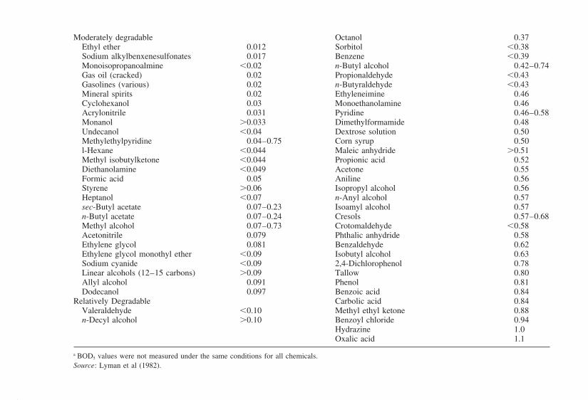
Moderately degradable Octanol 0.37Ethyl ether 0.012 Sorbitol 0.38Sodium alkylbenxenesulfonates 0.017 Benzene 0.39Monoisopropanoalmine 0.02 n-Butyl alcohol 0.42–0.74Gas oil (cracked) 0.02 Propionaldehyde 0.43Gasolines (various) 0.02 n-Butyraldehyde 0.43Mineral spirits 0.02 Ethyleneimine 0.46Cyclohexanol 0.03 Monoethanolamine 0.46Acrylonitrile 0.031 Pyridine 0.46–0.58Monanol 0.033 Dimethylformamide 0.48Undecanol 0.04 Dextrose solution 0.50Methylethylpyridine 0.04–0.75 Corn syrup 0.50l-Hexane 0.044 Maleic anhydride 0.51Methyl isobutylketone 0.044 Propionic acid 0.52Diethanolamine 0.049 Acetone 0.55Formic acid 0.05 Aniline 0.56Styrene 0.06 Isopropyl alcohol 0.56Heptanol 0.07 n-Anyl alcohol 0.57sec-Butyl acetate 0.07–0.23 Isoamyl alcohol 0.57n-Butyl acetate 0.07–0.24 Cresols 0.57–0.68Methyl alcohol 0.07–0.73 Crotomaldehyde 0.58Acetonitrile 0.079 Phthalic anhydride 0.58Ethylene glycol 0.081 Benzaldehyde 0.62Ethylene glycol monothyl ether 0.09 Isobutyl alcohol 0.63Sodium cyanide 0.09 2,4-Dichlorophenol 0.78Linear alcohols (12–15 carbons) 0.09 Tallow 0.80Allyl alcohol 0.091 Phenol 0.81Dodecanol 0.097 Benzoic acid 0.84

Relatively Degradable Carbolic acid 0.84Valeraldehyde 0.10 Methyl ethyl ketone 0.88n-Decyl alcohol 0.10 Benzoyl chloride 0.94

Hydrazine 1.0Oxalic acid 1.1

a BOD5 values were not measured under the same conditions for all chemicals.Source: Lyman et al (1982).

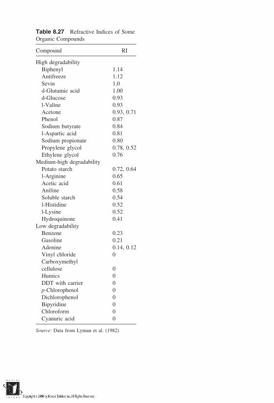
Table 8.27 Refractive Indices of SomeOrganic Compounds

Compound RI

High degradabilityBiphenyl 1.14Antifreeze 1.12Sevin 1.0d-Glutamic acid 1.00d-Glucose 0.93l-Valine 0.93Acetone 0.93, 0.71Phenol 0.87Sodium butyrate 0.84l-Aspartic acid 0.81Sodium propionate 0.80Propylene glycol 0.78, 0.52Ethylene glycol 0.76

Medium-high degradabilityPotato starch 0.72, 0.64l-Arginine 0.65Acetic acid 0.61Aniline 0.58Soluble starch 0.54l-Histidine 0.52l-Lysine 0.52Hydroquinone 0.41

Low degradabilityBenzene 0.23Gasoline 0.21Adenine 0.14, 0.12Vinyl chloride 0Carboxymethylcellulose 0Humics 0DDT with carrier 0p-Chlorophenol 0Dichlorophenol 0Bipyridine 0Chloroform 0Cyanuric acid 0

Source: Data from Lyman et al. (1982)

some of which may be preferentially biodegraded before others. The followinggeneral preference patterns (SCS, 1979; and U.S.EPA, 1996b) can be made:

Nonaromatics are preferentially biodegraded relative to aromatics.Unsaturated bonds in substances increase biodegradation potential.Straight-chain compounds can be biodegraded preferentially over

branched-chain compounds and others with more complex structuressuch as polymers.

Soluble compounds are more easily biodegraded than insoluble com-pounds.

Halogenated compounds tend to be more biorefractory than nonhaloge-nated compounds.

The presence of some functional groups in organic compounds enhancestheir biodegradability. For example, alcohols, aldehydes, acids, esters,amides, and amino acids are generally biodegradable.

8.13.2 Oxygen Requirements

Oxygen is required to degrade organic compounds at fast rates. However, anaero-bic biodegradation is also possible. The theoretical quantity of oxygen requiredto degrade organic compounds can be estimated through stoichiometry usingequations presented in Section 8.11. Oxygen can be supplied to microorganismsduring bioreclamation through any of the following methods: aeration, oxygen-ation, or use of compounds that can supply oxygen molecules. About 10 mg/liter of dissolved oxygen at 15°C is the maximum concentration that can be at-tained through injection of air. Sawyer and McCarty (1967) developed the follow-ing expression for estimating the quantity of dissolved oxygen in water:

C0 fPH (8.66)

where

C0 concentration of oxygen in water (mg/L)f volume fraction of oxygen in air (0.21)

P air pressure (atm)H Henry’s law constant for oxygen 43.8 (mg/L) • atm at 68°F

(20°C)

More oxygen can be transferred into solution through oxygenation systemsthan through aeration systems.

8.13.3 Groundwater Temperature

Generally, the bulk of soil bacteria are classified as mesophiles that grow wellwithin a temperature range of about 15–45°C. Additional classes of bacteria and

their preferred temperatures are psychrophiles (below 20°C) and thermophiles(45–65°C). Specific bacteria within these classes thrive in narrower temperatureranges within the wider ranges stated above. Generally, every 10°C increase intemperature doubles biotransformation rate.

8.13.4 Soil pH Conditions

A soil pH range of about 6–8 generally produces the greatest growth rate ofmicroorganisms, although most bacteria favor neutral pH conditions. Substancessuch as lime or acids can be introduced into soil systems to optimize bacterialgrowth.

8.13.5 Soil Nutrients

Microorganisms that degrade contaminants in soil need nutrients which are notnormally available completely in the target contaminants. These nutrients arerequired in specific proportions as matter for the synthesis of new cells duringbacterial growth. In their order of abundance, the typical composition of bacterialcells (on a dry-weight basis) are carbon (50%), oxygen (20%), nitrogen (14%),hydrogen (8%), phosphorus (3%), sulfur (1%), potassium (1%), sodium (1%),and calcium, magnesium, chlorine, iron, and other trace elements in percentagesthat are each less than 1%. The absence of one or more of these compounds maybe the limiting step in the growth of microorganisms and hence the effectivenessof the bioreclamation process.

Aerobic bioreclamation is more commonly employed than anaerobic biore-clamation in the in-situ bioremediation of contaminated subsurface media. Thisis because, at target sites, high concentration of organics generally require oxy-gen. A very brief quantitative description of the aerobic biodegradation kineticsin the aqueous environment based on Monod kinetics (Lyman et al., 1982) ispresented herein.

∂C∂t

kmaxCmC

Y(Ck C)(8.67)

where

∂(C )/∂t rate of disappearance of substratekmax maximum growth rate of microorganisms (number/T)Cm concentration of microorganisms (number/L)C concentration of substrate (M/L3)

Ck concentration of the substrate supporting half of themaximum growth rate, approximates 0.1–10 mg/liter formost substances (M/L3)

Y yield coefficient ∂Cm/∂C, approximates 0.5 fornondilute systems.

Two conditions can be stated and used to develop approximate estimates offinal contaminant concentrations for known growth rates and initial contaminantconcentrations. For CCk, which applies in the initial stages of bioreclamation,(Ck C ) can be assumed to be equal to C and eq. (8.67) can be manipulated toarrive at

Cf Ciekmaxt (8.68)

Cf final concentration of contaminant (M/L3)Ci initial concentration of contaminant (M/L3)

t time (T)kmax maximum growth rate of the microorganisms using first-order

rate constant (number/T)e base of natural logarithms

For C Ck, (Ck C ) approximates Ck. Then Eq. (8.67) becomes

∂C

∂t

kmaxCmC

YCk

(8.69)

The growth rate kmax can be estimated using methods described in standard micro-biology textbooks.

8.14 OTHER TECHNIQUES

Several other techniques, most of which have been used in ex-situ treatment ofcontaminated media, have been developed. Among these techniques are electroki-netic remediation, which involves the application of electrical energy to generatethe movement of charged components of contaminants in desired directions, ther-mal treatment, incinceration, and solvent extraction.

REFERENCES

Agrawal, A., and Tratnyek, P. G. 1996. Reduction of nitro aromatic compounds by zero-valent iron metal. Environmental Science and Technology, Vol. 30, pp. 153–160.

API. 1980. Underground Spill Cleanup Manual, API Publication 1628. American Petro-leum Institute, Washington, DC.

Baker, A. I. M., and Brooks, R. R. 1989. Terrestrial higher plants which hyperaccumulatemetallic elements: a review of their distribution, ecology, and phytochemistry. Bio-recovery, Vol. 1, pp. 81–126.

Bass, D. H. 1993. Estimation of effective cleanup radius for soil vapor extraction systems.Journal of Soi Contamination, Vol. 2, No. 2, pp. 191–202.

Chaung, F., Larson, R. A., and Wessman, M. S. 1995. Zero-valent iron-promoted dechlori-nation of polychlorinated biphenyls. Environmental Science and Technology, Vol.29, No. 9, pp. 2460–2463.

Crank, J. 1975. The Mathematics of Diffusion. Oxford University Press, London, England.Dorfman, L. M., and Adams, G. E. 1973. Reactivity of hydroxyl radical in aqueous solu-

tion. U.S. Department of Commerce, National Bureau of Standards, Washington,DC.

Eary, L. E., and Rai, D. 1988. Chromate removal from aqueous wastes by reduction withferrous iron. Environmental Science and Technology, Vol. 22, No. 8, pp. 972–977.

Gabr, M. A., Wang, J., and Bowders, J. J. 1996. Model for efficiency of soil flushingusing PVD-enhanced system. Journal of Geotechnical Engineering, Vol. 122, No.11, pp. 914–919.

Gierke, J. S., Wang, C., West, O. R., and Siegrist, R. L. 1995. In situ mixed region vaporstripping in low-permeability media. 3. Modeling of field tests. Environmental Sci-ence and Technology, Vol. 29, No. 9, pp. 2208–2216.

Hansen, J. E. 1991. Treatment of heavy metal contaminated soils by in situ vitrification.Presented at the 4th. Annual Hazardous Materials Management Conference, Rose-mont, IL, April 3–5.

Harris, J. C. 1982. Rate of hydrolysis. In: Handbook of Chemical Property Estimation (Lyman,W. J., Reehl, W. F., and Rosenblatt, O. H., eds.). McGraw-Hill, New York, chap. 7.

Heijman, C. G., Grieder, E., Hollinger, C., and Schwarzenbach, R. P. 1995. Reduction ofnitroaromatic compounds coupled to microbial iron reduction in laboratory aquifercolumns. Environmental Science and Technology, Vol. 29, pp. 775–783.

Huang, J. W., Chen, J., Berti, W. R., and Cunningham, S. D. 1997. Phytoremediation oflead-contaminated soils: role of synthetic chelates in lead phytoextraction. Environ-mental Science and Technology, Vol. 31, pp. 800–805.

Hunt, J., Sitar, N. and Udell, K. 1988. Nonaqueous phase liquid transport and cleanup: I.Analysis of mechanisms. Water Resources Research, Vol. 24, No. 8, pp. 1247–1258.

HWC. 1990. In situ vitrification update. Hazardous Waste Consultant, September/Octo-ber, pp. 1–18.

Johnson, P. C., Kemblowski, M. W., and Colthart, J. D. 1990. Quantitative analysis forthe cleanup of hydrocarbon contaminated soils by in-situ soil venting. Groundwater,Vol. 28, No. 3, pp. 413–429.

Kayano, S., and Wilson, D. J. 1993. Migration of pollutants in groundwater. VI. Flushingof DNAPL droplets/ganglia. Environmental Monitoring and Assessment, Vol. 25,pp. 193–212.

Keeley, J. F. 1989. Performance evaluations of pump-and-treat remediations, EPA Super-fund Groundwater Issue Document EPA/540/4-89/005. Office of Solid/Waste andEmergency Response, U.S. Environmental Protection Agency, Washington, DC.

Kerfoot, H. B. 1994. In situ determination of the rate of unassisted degradation of satu-rated-zone hydrocarbon contamination. Journal of Air and Waste Management As-sociation, Vol. 44, pp. 877–880.

Knox, R. C., Sabatini, D. A., and Canter, L. W. 1993. Subsurface Transport and FateProcesses. Lewis Publishers, Ann Arbor, MI.

LaGrega, M. D., and Evans, J. C. 1987. Overview of existing technologies for hazardouswaste site clean-up. Proceedings of the International Symposium on EnvironmentalGeotechnology, Allentown, PA, pp. 30–46.

Lingineni, S., and Dhir, V. K. 1992. Modeling of soil venting processes to remediateunsaturated soils. Journal of Environmental Engineering, Vol. 118, No. 1, pp. 135–151.

Lyman, W. J., Rechl, W. F., and Rosenblatt, O. H. 1982. Handbook of Chemical PropertyEstimation Methods. McGraw-Hill, New York.

Mabey, W., and Mill, T. 1978. Critical review of hydrolysis of organic compounds inwater environmental conditions. Journal of Physical Chemistry Reference Data,Vol. 7, No. 2, pp. 383–415.

Macdonald, J. A., and Kavanaugh, M. C. 1994. Restoring contaminated groundwater: anachievable goal? Environmental Science and Technology, Vol. 28, No. 8,pp. 362A–368A.

Masschelein, W. 1982. Ozonation Manual for Water and Wastewater Treatment. John,Wiley, New York.

McLellan, G. W., and Strand, E. B. 1984. Glass Engineering Handbook, 3rd ed. McGraw-Hill, New York.

Moffat, A.S. 1995. Plants proving their worth in toxic metal cleanup. Science, Vol. 269,pp. 302–303.

Newman, L. A., Strand, S. E., Choe, N., Duffy, J., Ekuan, G., Ruszaj, M., Shurtleff, B. B.,Wilmoth, J., Heilman, P., and Gordon, M. P. 1997. Uptake and biotransformation oftrichloroethylene by hybrid poplars. Environmental Science and Technology, Vol.31, pp. 1062–1067.

Nkedi-Kizza, P. Rao, P. S. C., and Hornsby, A. G. 1985. Influence of organic cosolventson sorption of hydrophobic organic chemicals by soils. Environmental Science andTechnology, Vol. 19, pp. 975–979.

O’Hannesin, S. F., and Gillham, R. W. 1993. In situ degradation of halogenated organicsby permeable reaction wall. Groundwater Currents, EPA/542/N-93/003, March.Office of Solid Waste and Emergency Response, U.S. Environmental ProtectionAgency, Washington, DC, pp. 1–2.

Orfeuil, M. 1987. Electric Process Heating. Battelle Press, Columbus, Richland, WA.Plodinec, M. J., Wicks, G. G., and Bibler, N. E. 1982. An assessment of Savannah River

borosilicate glass in repository environment, DP-1629. Savannah River Laboratory,Aiken, SC.

Radding, S. B., Liu, D. H., Johnson, H. L., and Mill, T. 1977. Review of the environmentalfate of selected chemicals, EPA 560/5-77-033. Office of Research and Develop-ment, U.S. Environmental Protection Agency, Washington, DC.

Ram, N. M., Bass, D. H., Falotico, R., and Leahy, M. 1993. A decision framework forselecting remediation technologies at hydrocarbon-contaminated sites. Journal ofSoil Contamination Vol. 2, No. 2, pp. 167–189.

Sawyer, C. N., and McCarty, P. L. 1967. Chemistry for Sanitary Engineers. McGraw-Hill, New York.

SCS. 1979. Selected biodegradation techniques for treatment and/or ultimate disposal oforganic materials, EPA-60/2-79-006. Soil Conservation Service, U.S. Environmen-tal Protection Agency, Cincinnati, OH.

Sivavec, T. M., and Horney, D. P. 1995. Reductive dechlorination of chlorinated ethenesby iron metal. Extended abstract presented at the American Chemical Society Meet-ing, Anaheim, CA, April 2–7.

Sivavec, T. M., Horney, D. P., and Baghel, S. S. 1995. Reductive dechlorination of chlori-nated ethenes by iron metal and iron sulfide minerals. Extended abstract presentedat the Industrial and Environmental Chemistry Special Symposium of the AmericanChemical Society, Atlanta, Georgia GA, September 17–20.

Tchobanoglous, G., and Schroeder, E. D. 1987. Water Quality, Addison-Wesley, Reading,MA, p. 286.

U.S. DOE. 1994. Summary report of a workshop on phytoremediation research needs,DOE/EM-0224. U.S. Department of Energy, Washington, DC.

U.S. EPA. 1986. Systems to accelerate in situ stabilization of waste deposits, EPA/540/2-86/002. Hazardous Waste Engineering Research Laboratory, U.S. EnvironmentalProtection Agency, Cincinnati, Ohio, OH.

U.S. EPA. 1987. A compendium of technologies used in the treatment of hazardouswastes, EPA/625/8-87/014. Center for Environmental Research Information, U.S.Environmental Protection Agency, Cincinnati, OH.

U.S. EPA. 1989a. Performance evaluations of pump-and-treat remediations. GroundwaterIssue, EPA/540/4-89/005. Office of Research and Development, U.S. Environmen-tal Protection Agency, Washington, DC.

U.S. EPA. 1989b. Stabilization/solidification of CERCLA and RCRA wastes: physicaltests, chemical testing procedures, technology screening, and field activities, EPA/625/6-89/022. Office of Research and Development, U.S. Environmental Protec-tion Agency, Washington, DC.

U.S. EPA. 1990. Basics of pump-and-treat groundwater remediation technology, EPA/600/8-90/003. Robert S. Kerr Environmental Research Laboratory, U.S. Environ-mental Protection Agency, Ada, OK.

U.S. EPA. 1992. Vitrification technologies for treatment of hazardous and radioactivewaste, EPA/625/R-92/002. Office of Research and Development, U.S. Environ-mental Protection Agency, Washington, DC.

U.S. EPA. 1992a. Chemical enhancements to pump-and-treat remediation (Palmer, C. D.,and Fish, W.), EPA/540/S-92/001. Office of Research and Development, U.S. En-vironmental Protection Agency, Washington, DC.

U.S. EPA. 1993. Remediation technologies screening matrix and reference guide, EPA-542-B-93-005. Office of Solid Waste and Emergency Response, U.S. Environmen-tal Protection Agency, Washington, DC.

U.S. EPA. 1994a. Superfund innovative technology evaluation program: technology pro-files, EPA/540/R-94/526. Office of Research and Development, U.S. Environmen-tal Protection Agency, Washington, DC.

U.S. EPA. 1994b. In situ vitrification treatment. Engineering Bulletin, EPA/540/S-94/504. Office of Research and Development, U.S. Environmental Protection Agency,Cincinnati, OH.

U.S. EPA. 1994c. Natural attenuation of hexavalent chromium in groundwater and soils.Ground Water Issue, EPA/540/S-94/505. Office of Research and Development,U.S. Environmental Protection Agency, Washington, DC.

U.S. EPA. 1995. How to evaluate alternative cleanup technologies for underground storage

tank sites, EPA/510-B-95-007. Office of Solid Waste and Emergency Response,U.S. Environmental Protection Agency, Washington, DC.

U.S. EPA. 1996a. Innovative treatment technologies: annual status report. Office of SolidWaste and Emergency Response, EPA-542-R-96-010, U.S. Environmental Protec-tion Agency, Washington, DC.

U.S. EPA. 1996b. A citizen’s guide to phytoremediation, EPA 542-F-96-014. Office ofSolid Waste and Emergency Response, U.S. Environmental Protection Agency,Washington, DC.

U.S. EPA. 1997. Recent developments for in situ treatment of metal contaminated soils,EPA-542-R-97-004. Office of Solid Waste and Emergency Response, U.S. Environ-mental Protection Agency, Washington, DC.

Versar, Inc. 1979. Water-related environmental fate of 129 priority pollutants, Vols. I andII, EPA/440-4-029a and b. U.S. Environmental Protection Agency, Washington,DC.

Volf, M. B. 1984. Chemical Approach to Glass. Elsevier, New York.Wilson, E. K. 1995. Zero-valent metals provide possible solution to groundwater prob-

lems. Chemical and Engineering News, July 3, pp. 19–22.Yang, Y. J., and Parker, R. A. 1998. Pump-and-treat systems. Chemical Engineering,

February, pp. 129–133.

9Containment SystemImplementation

9.1 ESSENTIALS OF WASTE CONTAINMENT

In Chapter 6, various mechanisms and scenarios of contaminant generation fromwastes were analyzed. This chapter focuses on approaches/techniques for con-taining such contaminants in the subsurface. Waste containment is one of thefour general approaches to waste management. The other approaches are wastetreatment (in situ or ex situ), natural attenuation, and waste excavation for dis-posal or recycling.

The contaminants that need to be contained can be present in the solid,liquid, or gaseous forms. In the subsurface, the liquid and gaseous-phase contami-nants are usually the focus of control efforts because of the relatively high mobil-ity of contaminants in these two phases. In this part of this text, the focus isprimarily on the liquid-phase contaminants, which generally migrate as a contam-inant plume in the subsurface. Wastes in the solid form could give rise to suchplumes through leaching processes described in Chapter 6. Waste containmentsystem components that can influence the rate of generation and migration ofleachates from waste solids are also analyzed. The volatile components of wastestend to migrate upward as permitted by the hydrogeological characteristics ofthe site concerned. Both active and passive collection schemes for vapor-phasecontaminants have been successfully implemented.

The implementation of effective schemes for waste containment requiresinformation on the size, shape, and directions of movement of the waste materialsand/or contaminants plume. For solid and liquid wastes that are stored in landfillsand impoundments/tanks, respectively, the size and shape can be inferred fromthe implemented design dimensions of the system. With respect to contaminant

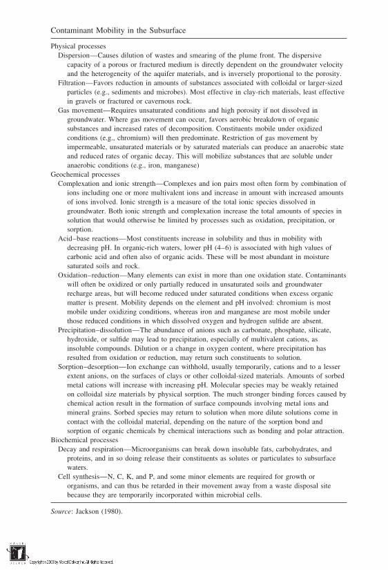
Contaminant Mobility in the Subsurface

Physical processesDispersion—Causes dilution of wastes and smearing of the plume front. The dispersive

capacity of a porous or fractured medium is directly dependent on the groundwater velocityand the heterogeneity of the aquifer materials, and is inversely proportional to the porosity.

Filtration—Favors reduction in amounts of substances associated with colloidal or larger-sizedparticles (e.g., sediments and microbes). Most effective in clay-rich materials, least effectivein gravels or fractured or cavernous rock.

Gas movement—Requires unsaturated conditions and high porosity if not dissolved ingroundwater. Where gas movement can occur, favors aerobic breakdown of organicsubstances and increased rates of decomposition. Constituents mobile under oxidizedconditions (e.g., chromium) will then predominate. Restriction of gas movement byimpermeable, unsaturated materials or by saturated materials can produce an anaerobic stateand reduced rates of organic decay. This will mobilize substances that are soluble underanaerobic conditions (e.g., iron, manganese)

Geochemical processesComplexation and ionic strength—Complexes and ion pairs most often form by combination of

ions including one or more multivalent ions and increase in amount with increased amountsof ions involved. Ionic strength is a measure of the total ionic species dissolved ingroundwater. Both ionic strength and complexation increase the total amounts of species insolution that would otherwise be limited by processes such as oxidation, precipitation, orsorption.

Acid–base reactions—Most constituents increase in solubility and thus in mobility withdecreasing pH. In organic-rich waters, lower pH (4–6) is associated with high values ofcarbonic acid and often also of organic acids. These will be most abundant in moisturesaturated soils and rock.

Oxidation–reduction—Many elements can exist in more than one oxidation state. Contaminantswill often be oxidized or only partially reduced in unsaturated soils and groundwaterrecharge areas, but will become reduced under saturated conditions when excess organicmatter is present. Mobility depends on the element and pH involved: chromium is mostmobile under oxidizing conditions, whereas iron and manganese are most mobile underthose reduced conditions in which dissolved oxygen and hydrogen sulfide are absent.

Precipitation–dissolution—The abundance of anions such as carbonate, phosphate, silicate,hydroxide, or sulfide may lead to precipitation, especially of multivalent cations, asinsoluble compounds. Dilution or a change in oxygen content, where precipitation hasresulted from oxidation or reduction, may return such constituents to solution.

Sorption–desorption—Ion exchange can withhold, usually temporarily, cations and to a lesserextent anions, on the surfaces of clays or other colloidal-sized materials. Amounts of sorbedmetal cations will increase with increasing pH. Molecular species may be weakly retainedon colloidal size materials by physical sorption. The much stronger binding forces caused bychemical action result in the formation of surface compounds involving metal ions andmineral grains. Sorbed species may return to solution when more dilute solutions come incontact with the colloidal material, depending on the nature of the sorption bond andsorption of organic chemicals by chemical interactions such as bonding and polar attraction.

Biochemical processesDecay and respiration—Microorganisms can break down insoluble fats, carbohydrates, and

proteins, and in so doing release their constituents as solutes or particulates to subsurfacewaters.

Cell synthesis—N, C, K, and P, and some minor elements are required for growth ororganisms, and can thus be retarded in their movement away from a waste disposal sitebecause they are temporarily incorporated within microbial cells.

Source: Jackson (1980).

plumes in the subsurface, there are uncertainties associated with the dimensionsand shape of the plume to be contained. Such uncertainties are due to their physi-cochemical characteristics and interactions among waste constituents, site hydro-geological parameters, and climatic factors. Table 9.1 shows a summary of theprimary physicochemical and biochemical factors that can influence the mobilityof aqueous phase contaminants in the subsurface (Jackson, 1980). Aquifer charac-teristics such as hydraulic conductivity and its spatial variability, proximity andfracture intensity of the bedrock, and soil stratification influence the size andshape of the contaminant plume as well. As shown in Table 9.2 (Freeze andCherry, 1979) various geomedia have widely different hydraulic conductivities.Assuming that other factors are constant, the rate of migration (hence, plumesize) is proportional to hydraulic conductivity. Figures 9.1–9.3 (U.S. EPA, 1985)illustrate the effects of subsurface hydrogeological conditions on plume shape.

In Figure 9.1, the contaminant is miscible with water and moves in a homo-geneous medium. In this relatively simple case, the plume is displaced laterallyby the transverse-flowing groundwater. The plume migration speed is essentiallythe composite speed of movement of the various contaminants that constitute theplume. If the geomedium is clayey, physicochemical and biological processeswill act to retard the migration of contaminants. For media that are dominatedby silts and sands, interactions are mostly in the physical realm: contaminant

Table 9.2 Typical Ranges of Hydraulic Conductivity Values ofGeomedia

Hydraulic conductivity

Geologic material cm/s gal/day/ft2

Gravel 101–102 104–107

Sand, well sorted 104–1 10–105

Silty sand 105–101 1–104

Silt 107–103 102–102

Clay, unweathered 1010–107 105–102

Glacial till 1010–104 105–10Carbonate rocks 107–1 103–105

Sandstones 108–104 103–10Shales 1011–107 106–102

Crystalline rocksHighly fractured 106–1 101–105

Relative unfractured 1012–108 107–103

1 gal/day/ft2 1.74 106 ft/day1 gal/day/ft2 4.72 105 cm/sSource: Freeze and Cherry (1979).

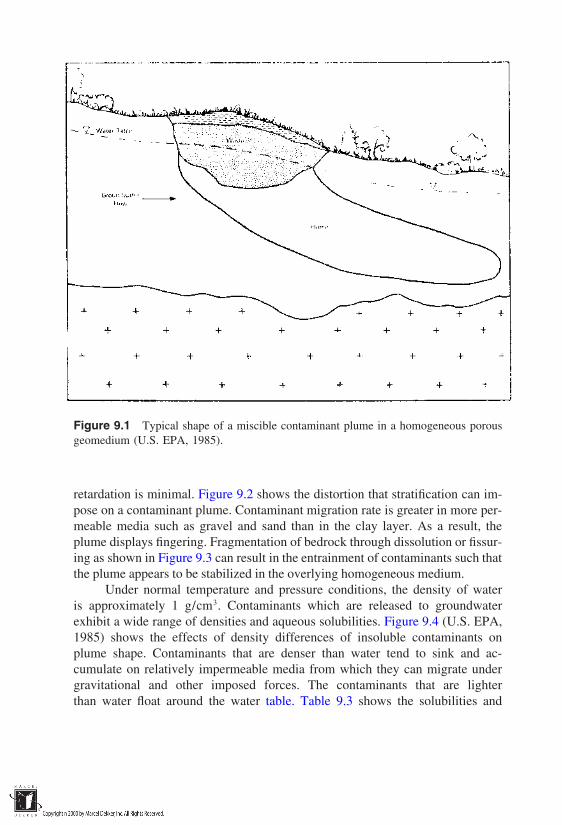
Figure 9.1 Typical shape of a miscible contaminant plume in a homogeneous porousgeomedium (U.S. EPA, 1985).

retardation is minimal. Figure 9.2 shows the distortion that stratification can im-pose on a contaminant plume. Contaminant migration rate is greater in more per-meable media such as gravel and sand than in the clay layer. As a result, theplume displays fingering. Fragmentation of bedrock through dissolution or fissur-ing as shown in Figure 9.3 can result in the entrainment of contaminants such thatthe plume appears to be stabilized in the overlying homogeneous medium.

Under normal temperature and pressure conditions, the density of wateris approximately 1 g/cm3. Contaminants which are released to groundwaterexhibit a wide range of densities and aqueous solubilities. Figure 9.4 (U.S. EPA,1985) shows the effects of density differences of insoluble contaminants onplume shape. Contaminants that are denser than water tend to sink and ac-cumulate on relatively impermeable media from which they can migrate undergravitational and other imposed forces. The contaminants that are lighterthan water float around the water table. Table 9.3 shows the solubilities and

Figure 9.2 Effects of geomedia stratification on contaminant plume. (U.S. EPA, 1985).

densities of some common contaminants. Knowledge about the distribution ofvarious contaminants within a plume is important in the design of containmentschemes.

The primary functions of waste containment systems fall into the followingcategories:

Minimization of the intrusion of moisture, which can generate and mobilizeleachate

Minimization of the transport of waste constituents into the surroundingenvironment

Isolation of wastes such that the potential for contact by humans and otheranimals is minimized

More specific design functions of various types of containment systems arediscussed in Chapter 10.

Figure 9.3 Effects of secondary porosity on contaminant plume movement (U.S. EPA,1985).

9.2 HYDRAULIC AND PHYSICAL CONTAINMENT

Waste constituents and moisture can be contained through the installation of bar-riers or pore fluid extraction through gravity-induced drainage or pumping. Theconfigurations of physical containment systems are presented and discussedin Chapter 10. Also, numerical techniques for assessing their structural stabil-ity and moisture/contaminant transport through their components are dis-cussed in Chapter 11.

Physical containment involves the installation of barriers to attenuate con-taminants, and/or change their direction and/or rate of transport in the subsurface.Attenuation can be accomplished through the use of sorptive, low-permeabilitymaterials, or permeable, but reactive materials. In both cases, the objective is toreduce output concentration, with respect to the input concentration of the tar-geted contaminants. In the case of permeable barriers, the flow rate of moisture

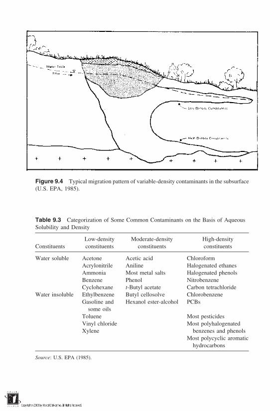
Figure 9.4 Typical migration pattern of variable-density contaminants in the subsurface(U.S. EPA, 1985).

Table 9.3 Categorization of Some Common Contaminants on the Basis of AqueousSolubility and Density

Low-density Moderate-density High-densityConstituents constituents constituents constituents

Water soluble Acetone Acetic acid ChloroformAcrylonitrile Aniline Halogenated ethanesAmmonia Most metal salts Halogenated phenolsBenzene Phenol NitrobenzeneCyclohexane t-Butyl acetate Carbon tetrachloride

Water insoluble Ethylbenzene Butyl cellosolve ChlorobenzeneGasoline and Hexanol ester-alcohol PCBs

some oilsToluene Most pesticidesVinyl chloride Most polyhalogenated

benzenes and phenolsXyleneMost polycyclic aromatic

hydrocarbons

Source: U.S. EPA (1985).

Table 9.4 Contaminant Plume Characteristics that Should Be Considered in the Selection of Leachate Migration Control Techniques

Leachate migration control technologies

Low-permeabilityPlume characteristic Groundwater pumping Subsurface drains barriers In-situ treatment

Viscosity Highly viscous leachate Highly viscous leachate Little or no effect Effect depends on the de-may clog screens, may clog envelope ma- livery system usedpipes, and pumps thus terials, resulting inreducing well efficiency drain failure

Solubility in Pumping systems can be Drainage systems can be Little or no effect Effect depends on thegroundwater designed for both solu- designed for both solu- treatment technology

ble and insoluble con- ble and insoluble con- usedtaminants taminants, although

drains tend to functionmore effectively whencontaminants are solu-ble in groundwater

Reactiveness, explo- Care must be taken during Care must be taken during Care must be taken during Care must be taken in in-siveness, corro- installation and the oper- installation and the oper- installation; some con- plementing in-situ treat-siveness, vola- ation of pumps and ation of pumps and taminants may degrade ment activities. The abil-tility treatment systems; treatment systems; wall materials ity of contaminants to

some contaminants may some contaminants may enter into chemical anddegrade well materials degrade drain materials biochemical reactions,

however, is a require-ment of in-situ treat-ment technologies.

Toxicity Little or no effect except Little or no effect except Little or no effect Effect depends on thefor treatment system for treatment system treatment technique

used; some highly toxiccontaminants cannot bebioreclaimed

Flow direction Little or no effect because Little or no effect because Very important for plac- Little or no effectthe system will readjust the system will readjust ing noncircumferentialflow direction flow directions walls especially if flow di-

rections change seasonallyFlow rate Important in system de- High flow rates generally Can be very important for Can be very important de-

sign and operation but gen- preclude the use of subsur- noncircumferential walls pending on the treatmenterally does not affect se- face drains especially downgradient system usedlection or performance walls

Volume and extent Little or no effect Generally not practical for Generally not practical for Generally not practical forvery large plumes isolating very large very large plumes

plumesContaminant types Can affect the selection of Can affect the selection of Can affect wall placement Generally the primary con-

system materials and com- system materials and com- and performance if con- sideration in selecting aponents; some contami- ponents; some contami- taminants degrade wall treatment systemnants can clog systems nants can clog systems materials

Concentrations Little or no effect if the High concentrations of High concentrations of High contaminant concen-system is designed and op- some contaminants will some contaminants can de- trations cannot be treatederated properly clog drainage systems grade wall materials effectively by some treat-

ment systemsDensity Will influence the place- Can reduce system effec- Very important for hang- May be a factor in the de-

ment of screens in individ- tiveness if drain is not situ- ing walls sign of the deliveryual wells ated properly within the system

aquifer

Source: U.S. EPA (1985).

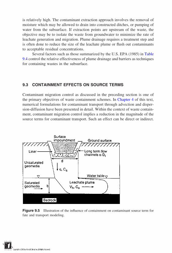
is relatively high. The contaminant extraction approach involves the removal ofmoisture which may be allowed to drain into constructed ditches, or pumping ofwater from the subsurface. If extraction points are upstream of the waste, theobjective may be to isolate the waste from groundwater to minimize the rate ofleachate generation and migration. Plume drainage requires a treatment step andis often done to reduce the size of the leachate plume or flush out contaminantsto acceptable residual concentrations.

Several factors such as those summarized by the U.S. EPA (1985) in Table9.4 control the relative effectiveness of plume drainage and barriers as techniquesfor containing wastes in the subsurface.

9.3 CONTAINMENT EFFECTS ON SOURCE TERMS

Contaminant migration control as discussed in the preceding section is one ofthe primary objectives of waste containment schemes. In Chapter 4 of this text,numerical formulations for contaminant transport through advection and disper-sion-diffusion have been presented in detail. Within the context of waste contain-ment, contaminant migration control implies a reduction in the magnitude of thesource terms for contaminant transport. Such an effect can be direct or indirect.

Figure 9.5 Illustration of the influence of containment on contaminant source term forfate and transport modeling.

Table 9.5 Factors that Influence Leachate Generation from Buried orContained Waste

Factor Effect

PrecipitationAmount per year The greater the amount of precipitation, the greater the vol-

ume of leachate generated.Highest 24-h rainfall No real effect, but the greater the number of short-dura-

tion, high-volume rainstorms, the less likely that precipi-tation will infiltrate to waste, and the more likely thatmost will run off as surface flow.

Mean annual temperature The higher the mean annual temperature, the greater theamount of precipitation that will evaporate and not infil-trate into waste, reducing the volume of leachate genera-tion.

Degree of insolation Increasing insolation will increase evaporation, reducingthe quantity of leachate produced.

Surface slope Increasing slope at a disposal site will promote surface run-off, reducing the volume of precipitation infiltrating intothe waste and thus reducing the volume of leachate gen-erated.

Cover permeability Low-permeability cover materials promote runoff, reducinginfiltration and the volume of leachate generated.

Vegetation Heavy vegetative cover of grasses will increase transpira-tion. Heavy vegetative cover of grasses can also impederunoff, thus increasing infiltration.

Heavy vegetative cover of trees, bushes, and shrubs may in-crease infiltration by opening up channels of flow intowaste because of deep root penetration.

Subsurface characteristicsWater content of waste Increased water content within waste will decrease time

until leachate generation begins.Volume of water flow Increased water flow through waste will increase the vol-

through waste ume of leachate generated.Rate of flow through Increased flow rates through waste will decrease time until

wastes start of leachate generation, but may decrease the con-centration of contaminates present.

Source: U.S. EPA (1985).

An indirect effect is the minimization of infiltration rate of moisture, which inturn reduces the leachate production rate. A direct effect is the containment ofthe leachate, which reduces in its concentration at the clean side of the barrierand possibly reduces the fluid flow rate through the barrier.

An example of the direct effect is illustrated for a lined surface im-poundment in Figure 9.5. The source term concentration, Co, shown in the figure,is nominally related to the other parameters as follows:

Co Caqd

Vhb(9.1)

where

Co source term concentration per unit width of the plume, forcontaminant fate and transport modeling (M/L2)

q contaminant flow rate per unit width in the unsaturated zone(L2/T)

Ca contaminant concentration in the vadose zone (M/L3)d width of the satureate zone (L)

Vh plume velocity (L/T)b plume thickness (L)

The liner influences both q and Ca, which are partial determinants of Co.Covers are the most common means of controlling source terms indirectly.

In this regard the essential function is minimization of the infiltration rate ofmoisture. The factors that influence the effectiveness of the infiltration controlapproach are presented in Table 9.5 (after U.S. EPA, 1985). Barrier systemsare not perfect and tend to deteriorate as time progresses, especially the buriedcomponents. Also, contaminant transport through nondegraded low permeabilitybarriers is slow but certain. Consequently, contaminant transport source termsare time-variable, as discussed and illustrated in Chapter 12.

9.4 CONTAINMENT SITE SELECTION TECHNIQUES

Site factors are important in waste containment because of the following reasons.

Hydrological and hydrogeological factors which influence the performanceof a containment system vary from one site to another.

Some sites are more sensitive ecologically than others. Thus, for the samelevel of intrinsic performance of a containment system, the potential fordamage of a sensitive environment may be site-dependent.

For some waste containment scenarios, the site is already fixed. The option selec-tion issue centers around alternative techniques for containment. For other scenar-ios, the waste management site has to be selected on the basis of engineeringfactors, socioeconomic factors, environmental factors, and direct cost. Severalmethods (Mustalish and Costanzo, 1991; Bain and Hanse, 1981; Charnpratheepet al., 1997; Anandalingam and Westfall, 1989; Lemme et al., 1990; Vita, 1987;and Aller et al., 1985) that incorporate one or more of the categories of factorsmentioned above have been developed and used for facility site selection. Thecomprehensive site selection process illustrated in Figure 9.6 was applied byArmour (1986) to screen 150 candidate sites progressively to 8 and 6, beforeselecting a single site for a waste management facility in Alberta, Canada.

Assessment of technical factors in site selection for waste managementusually involves an analysis of the vulnerability and/or risk-mitigation capacitiesof the alternative sites. For the case of a location near Lake Poinsette, South

Figure 9.6 Example of a comprehensive site selection process for waste managementfacilities (Armour, 1986).

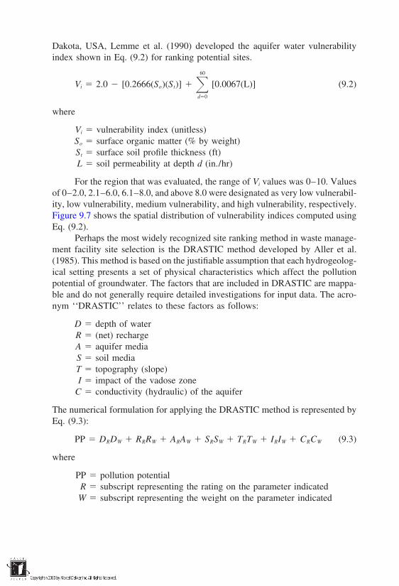
Dakota, USA, Lemme et al. (1990) developed the aquifer water vulnerabilityindex shown in Eq. (9.2) for ranking potential sites.

Vi 2.0 [0.2666(So)(St)] 60

d0

[0.0067(L)] (9.2)

where

Vi vulnerability index (unitless)So surface organic matter (% by weight)St surface soil profile thickness (ft)L soil permeability at depth d (in./hr)

For the region that was evaluated, the range of Vi values was 0–10. Valuesof 0–2.0, 2.1–6.0, 6.1–8.0, and above 8.0 were designated as very low vulnerabil-ity, low vulnerability, medium vulnerability, and high vulnerability, respectively.Figure 9.7 shows the spatial distribution of vulnerability indices computed usingEq. (9.2).

Perhaps the most widely recognized site ranking method in waste manage-ment facility site selection is the DRASTIC method developed by Aller et al.(1985). This method is based on the justifiable assumption that each hydrogeolog-ical setting presents a set of physical characteristics which affect the pollutionpotential of groundwater. The factors that are included in DRASTIC are mappa-ble and do not generally require detailed investigations for input data. The acro-nym ‘‘DRASTIC’’ relates to these factors as follows:

D depth of waterR (net) rechargeA aquifer mediaS soil mediaT topography (slope)I impact of the vadose zone

C conductivity (hydraulic) of the aquifer

The numerical formulation for applying the DRASTIC method is represented byEq. (9.3):

PP DRDW RRRW ARAW SRSW TRTW IRIW CRCW (9.3)

where

PP pollution potentialR subscript representing the rating on the parameter indicatedW subscript representing the weight on the parameter indicated

Figure 9.7 Aquifer vulnerability map of the Lake Poinsett Region of South Dakota,USA (Lemme et al. 1990).

Three categories of parameters (two direct and one indirect) determine themagnitude of PP. These categories are weight, ranges, and ratings. DRASTICfactors are weighted on a scale of 1–5 in direct proportion to the significance ofeach factor, relative to others. These weights are constant and are shown in Table9.6. The magnitude of each factor has been divided into ranges or characteristicmagnitudes and is supplied on each factor for various media. Each of the factors

Table 9.6 Weights Assigned to DRASTIC Factors

Feature Weight

Depth to water table 5Net recharge 4Aquifer media 3Soil media 2Topography 1Impact of the vadose zone 5Hydraulic conductivity of the aquifer 3

Note: The weights do not change. Source: Aller et al. (1985).

D, R, S, T, and C is assigned one specific value per range within the possiblemagnitude spectrum. For A and I, opportunity is allowed for the evaluator tochoose a typical value or a refined value on the basis of more precise informationabout the sites evaluated. Rating schemes for various DRASTIC factors are pre-sented in Tables 9.7–9.13. Table 9.14 illustrates the application of the DRASTICmethod to a site for which data on the parameters are presented. It should benoted that rating schemes such as DRASTIC are useful only for screening-levelanalysis of sites. More detailed analyses require more specific site data and detailson the design of the facility to be sited.

More elaborate site selection models have been developed. Among thesemodels are the fuzzy set/analytic hierarchy method (Charnpratheep et al., 1997)

Table 9.7 DRASTIC Ranges andRatings for Depth to Groundwater

Depth to water (ft)

Range Rating

0–5 105–10 915–30 730–50 550–75 375–100 2100 1

Weight: 5 Agricultural weight: 5

Source: Aller et al. (1985).

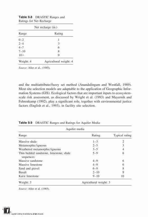
Table 9.8 DRASTIC Ranges andRatings for Net Recharge

Net recharge (in.)

Range Rating

0–2 12–4 34–7 67–10 810 9

Weight: 4 Agricultural weight: 4

Source: Aller et al., (1985).

and the multiattribute/fuzzy set method (Anandalingam and Westfall, 1989).Most site selection models are adaptable to the application of Geographic Infor-mation Systems (GIS). Ecological factors that are important inputs to ecosystem-scale risk assessment, as discussed by Wright et al. (1993) and Mayernik andFehrenkamp (1992), play a significant role, together with environmental justicefactors (English et al., 1993), in facility site selection.

Table 9.9 DRASTIC Ranges and Ratings for Aquifer Media

Aquifer media

Range Rating Typical rating

Massive shale 1–3 2Metamorphic/igneous 2–5 3Weathered metamorphic/igneous 3–5 4Thin bedded sandstone, limestone, shale 5–9 6

sequencesMassive sandstone 4–9 6Massive limestone 4–9 6Sand and gravel 6–9 8Basalt 2–10 9Karst limestone 9–10 10

Weight: 3 Agricultural weight: 3

Source: Aller et al. (1985).

Table 9.10 DRASTIC Ranges and Ratings for Soil Media

Soil media

Range Rating

Thin or absent 10Gravel 10Sand 9Shrinking and/or aggregated clay 7Sandy loam 6Loam 5Silty loam 4Clay loam 3Nonshrinking and nonaggregated clay 1

Weight: 2 Agricultural weight: 5

Source: Aller et al. (1985).

9.5 CONTAINMENT SITE IMPROVEMENT

The first option is usually to avoid sites that are not suitable for location of wastecontainment systems. From the standpoint of engineering and environmental pro-tection, suitable sites are those in which the present and future costs of implement-ing an effective control scheme for contaminants are acceptable. It is worth notingthat some of the costs may not be readily quantifiable in financial terms. In somecases, the contaminant plume exists already. The containment objective may be

Table 9.11 DRASTIC Ranges andRatings for Topography

Topography (percent slope)

Range Rating

0–2 102–6 96–12 512–18 318 1

Weight: 1 Agricultural weight: 3

Source: Aller et al. (1985).

Table 9.12 DRASTIC Ranges and Ratings for Impact of the Vadose Zone Media

Impact of vadose zone media

Range Rating Typical rating

Silt/clay 1–2 1Shale 2–5 3Limestone 2–7 6Sandstone 4–8 6Bedded limestone, sandstone, shale 4–8 6Sand and gravel with significant silt and clay 4–8 6Metamorphic/igneous 2–8 4Sand and gravel 6–9 8Basalt 2–10 9Karst limestone 8–10 10

Weight: 5 Agricultural weight: 4

Source: Aller et al. (1985).

focused on minimizing the rate of plume movement in the subsurface. In othercases, such as landfill siting, it may be necessary to implement a redundant con-tainment scheme for control of leachate that may be generated by the landfill.

The analysis presented in detail in Chapter 11 indicates that the contaminanttransport rate through porous media (such as those present in the subsurface) isdirectly proportional to the permeability of the media. The Kozeny relationship,

Table 9.13 DRASTIC Ranges andRatings for Hydraulic Conductivity

Hydraulic conductivity (gpd/ft2)

Range Rating

1–100 1100–300 2300–700 4700–1000 61000–2000 82000 10

Weight: 3 Agricultural weight: 2

Source: Aller et al. (1985).

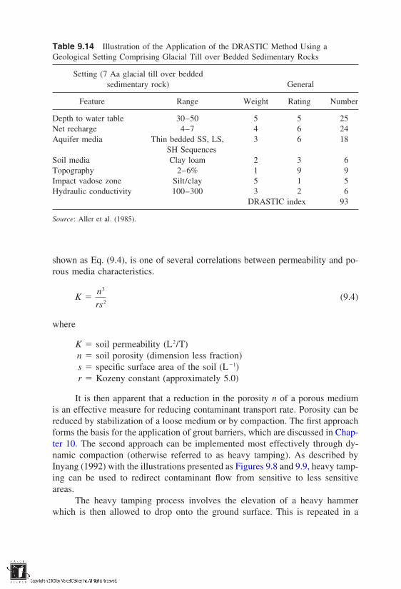
Table 9.14 Illustration of the Application of the DRASTIC Method Using aGeological Setting Comprising Glacial Till over Bedded Sedimentary Rocks

Setting (7 Aa glacial till over beddedsedimentary rock) General

Feature Range Weight Rating Number

Depth to water table 30–50 5 5 25Net recharge 4–7 4 6 24Aquifer media Thin bedded SS, LS, 3 6 18

SH SequencesSoil media Clay loam 2 3 6Topography 2–6% 1 9 9Impact vadose zone Silt/clay 5 1 5Hydraulic conductivity 100–300 3 2 6

DRASTIC index 93

Source: Aller et al. (1985).

shown as Eq. (9.4), is one of several correlations between permeability and po-rous media characteristics.

K n3

rs2(9.4)

where

K soil permeability (L2/T)n soil porosity (dimension less fraction)s specific surface area of the soil (L1)r Kozeny constant (approximately 5.0)

It is then apparent that a reduction in the porosity n of a porous mediumis an effective measure for reducing contaminant transport rate. Porosity can bereduced by stabilization of a loose medium or by compaction. The first approachforms the basis for the application of grout barriers, which are discussed in Chap-ter 10. The second approach can be implemented most effectively through dy-namic compaction (otherwise referred to as heavy tamping). As described byInyang (1992) with the illustrations presented as Figures 9.8 and 9.9, heavy tamp-ing can be used to redirect contaminant flow from sensitive to less sensitiveareas.

The heavy tamping process involves the elevation of a heavy hammerwhich is then allowed to drop onto the ground surface. This is repeated in a

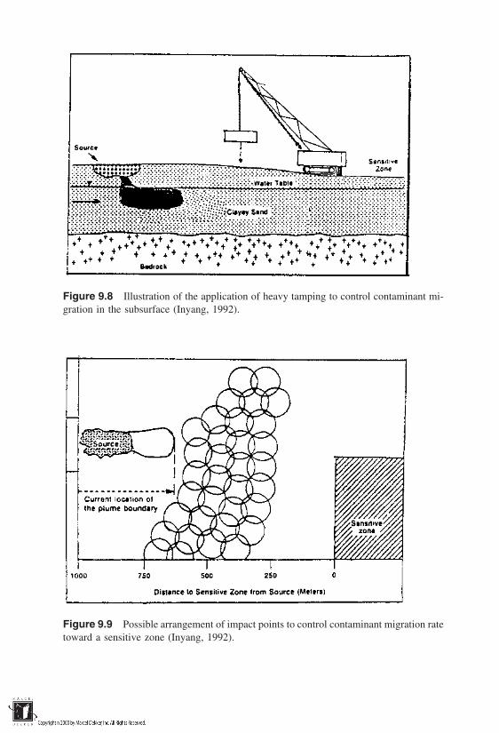
Figure 9.8 Illustration of the application of heavy tamping to control contaminant mi-gration in the subsurface (Inyang, 1992).

Figure 9.9 Possible arrangement of impact points to control contaminant migration ratetoward a sensitive zone (Inyang, 1992).

suitable pattern until the soil is adequately densified. The energy imposed by thehammer on the soil medium is dissipated through the following processes, therelative intensities of which vary by soil type, energy level, and degree of satura-tion:

Elastic wave propagationPlastic compression of soilCrushing of soil particlesPore pressure buildup in soil

In essence, the soil particles are shaken to a denser structure even at loca-tions that may be several meters away from the zone of hammer contact. Typicalranges of magnitudes for dynamic compaction parameters are presented in Table9.15. Some relationships among these parameters have been proposed by Menardand Broise (1975), and by Charles et al. (1981), as shown in Eqs. (9.5) and (9.6),respectively. Both relationships can be used to estimate the depth of influenceof the hammer force for a given set of soil strength, hammer weight, and dropheight values.

Table 9.15 Suggested Numerical Ranges of Heavy Tamping Design Factors forContaminant Migration Rate Control

NumericalFactor range Comments

Required depth of compaction (m) 12 Depends on the thickness of theloose layer

Applied impact energy energy 200–300 Applied impact energy depends on(measure-m/m2) specified improvement in relativeTamper diameter (m) 1.0–3.0 density of soilDrop height (m) 10–30Drop weight (tonnes) 5–40

Repetitions (impacts per point) 2–8 Depends on specified improvementin relative density

Spacing of impact points (m) 1.0–4.0 Depends on desired overlap of thetributary areas

Minimum depth to water table (m) 2.0–3.0 Temporary dewatering may be re-quired to attain this condition

Required improvement in relative 40 Depends on desired decrease in soildensity (%) permeabilityPeak particle velocity at nearby 4.0 Should be evaluated prior to full-

structures (cm/s) scale project implementation

Source: Inyang (1992).

D R (WH )0.5 (9.5)

D 0.4d E

A 1d 1

c0.5

(9.6)

where

D depth of soil improvement (L)R empirical factor that depends on soil type, ranging from about

0.35 for fine-grained soils to 0.6 for granular free-draining soils;0.5 is frequently used as an approximate value

W weight of hammer (g)h hammer drop height (L)d diameter of hammer (L)E applied impact energy (g-L)A area of impact (L2)C undrained shear strength of soil (g/L2)

It should be noted that dynamic compaction may not always produce a permanentbarrier to contaminant migration.

REFERENCES

Aller, L., Bennett, T., Lehr, J. H., and Petty, R. J. (1985). DRASTIC: A standardizedsystem for evaluating groundwater pollution potential using hydrogeologic settings.Technical Report under Cooperative Agreement CX-819715-01, Office of Researchand Development, U.S. Environmental Protection Agency, Ada, Oklahoma, UK.

Anandalingam, G., and Westfall, M. (1989). Selection of hazardous waste disposal alterna-tive using multi-attribute utility theory and fuzzy set analysis. J. Environ. Syst.,18(1):69–85.

Armour, A. (1986). Social impact assessment of new hazardous waste facilities. Technicaldocument developed for the Hazardous Waste Facilities Siting Board, Annapolis,MD.

Bain, G. L., and Hansen, P. (1981). Geologic and hydrologic implications of hazardouswastes management rules on siting in North Carolina. Bull. Assoc. Eng. Geol.,XVIII(3):267–275.

Charles, J. A., Burford, D., and Watts, K. S. (1981). Field studies of the effectiveness ofdynamic consolidation. Proc. 10th Int. Conf. on Soil Mechanics and FoundationEngineering, I. Stockholm, pp. 617–622.

Charnpratheep, K., Zhou, Q., and Garner, B. (1997). Preliminary landfill site screeningusing fuzzy geographical information systems. Waste Manage. Res., 15:197–215.

English, M., Barkenbus, J., and Wilt, C. (1993). Solid waste facility siting: Issues andtrends. J. Air Waste Manage. Assoc., 43:1345–1350.

Freeze, R. A., and Cherry, J. A. (1979). Groundwater. Prentice-Hall, Englwood Cliffs,NJ.

Inyang, H. I. (1992). Application of dynamic compaction to contaminant migration con-trol. Proc. 13th Annual Natl. Conf. and Exhibition on Hazardous Materials Control,Washington, DC, pp. 625–630.

Jackson, R. E. (1980). Aquifer contamination and protection. Project 8.3 of the Interna-tional Hydrological Programme, United Nations Educational, Scientific and Cul-tural Organization, Paris, France.

Lemme, G., Carlson, C. G., Dean, R., and Khakurai, B. (1990). Contamination vulnerabil-ity indexes: A water quality planning tool. J. Soil Water Conserv., March–April:349–350.

Mayernik, J. A., and Fehrenkamp, K. (1992). A new model for conducting quantitativeecological risk assessments at hazardous waste sites. Proc. 13th Annual Natl. Conf.on Hazardous Materials Control, Washington, DC, pp. 813–819.

Menard, L., and Broise, Y. (1975). Theoretical and practical aspects of dynamic consolida-tion. Geotechnique, 25(1):3–18.

Mustalish, R. W., and Costanzo, F. (1991). An application of the DRASTIC model to thesiting of waste facilities. Proc. 12th Natl. Conf. on Hazardous Materials Control,Washington, DC, pp. 51–53.

U.S. EPA. (1985). Leachate plume management, EPA/540/2-85/004. Office of Emer-gency and Remedial Response, U.S. Environmental Protection Agency, Washing-ton, DC.

Vita, C. L. (1987). Generalized risk-based decision making for hazardous waste sites.Proc. Natl. Conf. on Hazardous Wastes and Hazardous Materials, Washington,DC, pp. 32–37.

Wright, F. G., Inyang, H. I., and Myers, V. B. (1993). Risk reduction through regulatorycontrol of waste disposal facility siting. J. Environ. Syst. 22(1):27–35.

10Configurations of ContainmentSystems

The configuration of a containment system for wastes plays a significant rolewith respect to the effectiveness of the system in meeting its design functionduring the design life. Essentially, configuration is the arrangement of the compo-nents of the system. It influences the extent to which the components are exposedto environmental stresses, contaminant and moisture contact, and anthropogenicactivities. Also, the configuration of components within a multicomponent systemaffects the distribution and propagation of stresses and deformation from onecomponent to another. The objective of this chapter is to introduce the reader tothe most common configurations of waste containment systems. Design ap-proaches and quantitative expressions for various components of containmentsystems are provided in Chapters 9, 11, and 12.

10.1 LANDFILLS

In general, the overall design goal of landfills is minimization of the release ofstored hazardous materials into the environment. Two design approaches tie inwith this goal:

Minimization of the quantity of leachates generated within the landfillthrough adequate design of the cover system and surface drainage com-ponents

Minimization of the quantity of hazardous materials that migrate from thelandfill into the environment through the incorporation of well-designedliners and leachate collection systems below the stored waste

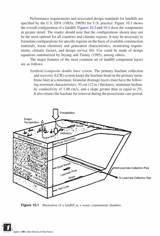
Performance requirements and associated design standards for landfills arespecified by the U.S. EPA (1985a, 1985b) for U.S. practice. Figure 10.1 showsthe overall configuration of a landfill. Figures 10.2 and 10.3 show the componentsin greater detail. The reader should note that the configurations shown may notbe the most optimal for all countries and climatic regions. It may be necessary toformulate configurations for specific regions on the basis of available constructionmaterials, waste chemistry and generation characteristics, monitoring require-ments, climatic factors, and design service life. Use could be made of designequations summarized by Inyang and Tumay (1995), among others.

The major features of the most common set of landfill component layersare as follows.

Synthetic/composite double liner system. The primary leachate collectionand recovery (LCR) system keeps the leachate head on the primary mem-brane liner at a minimum. Granular drainage layers must have the follow-ing minimum characteristics: 30 cm (12 in.) thickness, minimum hydrau-lic conductivity of 1.00 cm/s, and a slope greater than or equal to 2%.It also retains the leachate for removal during the postclosure care period.

Figure 10.1 Illustration of a landfill as a waste containment chamber.

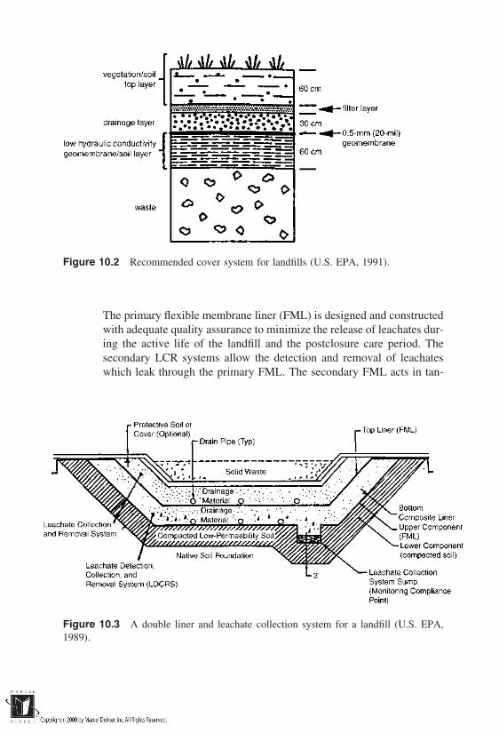
Figure 10.2 Recommended cover system for landfills (U.S. EPA, 1991).

The primary flexible membrane liner (FML) is designed and constructedwith adequate quality assurance to minimize the release of leachates dur-ing the active life of the landfill and the postclosure care period. Thesecondary LCR systems allow the detection and removal of leachateswhich leak through the primary FML. The secondary FML acts in tan-

Figure 10.3 A double liner and leachate collection system for a landfill (U.S. EPA,1989).

dem with the compacted clay liner to prevent the release of leachates inquantities that exceed specified limits.

Synthetic/clay double liner system. The leachate collection systems servethe same functions as described above. However, only one FML layeris incorporated. A clay liner is included, the thickness of which dependson the calculated breakthrough time for a single leachate constituent topass from the top of the clay liner.

As illustrated in Figure 10.2, the cover system is multilayered. It is usuallydesigned to promote surface drainage, withstand waste settlement, and accom-modate soil profile subsidence. The top vegetative cover is intended to mini-mize erosion and promote evapotranspiration. An optional gas collectionlayer may be incorporated. A low-permeability clay layer (at least 2 ft thick)and a 20-mil flexible membrane cap (FMC) are also included. On top of theFMC, a surface-water drainage layer is usually placed. It may consist of threecomponents: a bedding layer which protects the FMC; the actual drainage layer;and a filter layer that prevents the intrusion of vegetative cover soil intothe drainage component.

Additional literature that addresses various design and service aspects oflandfill components are Haikola et al. (1995), Bonaparte (1995), Benson andOthman (1993), Inyang (1994), Inyang et al. (1997a, 1997b), Koerner (1990),Richardson and Koerner (1989), Ware and Jackson (1978), Duvel (1979), Reidet al. (1971), Thornton and Blackwell (1976), Weston (1989), Emcon Associates(1982), Haxo (1980), Hughes (1975), Cope (1987), Koerner and Whitty (1984),Duplancic (1987), Goodall and Quigley (1987), Giroud and Ah-Line (1984),Cosler and Snow (1984), Glebs (1980), Gordon and Huebner (1983), Quinn(1983), and Bass et al. (1984).

10.2 SLURRY WALLS

Slurry walls are subsurface trenches that are filled with low-permeability soilmaterials and possibly other additives to retard the migration of contaminantsinto the surrounding soil/groundwater environment. Slurry walls are particularlyuseful in loose subsurface materials, where they can divert uncontaminatedgroundwater away from waste or contaminant plume, reduce the flow rate ofleachate into the subsurface, increase the retardation or decay of contaminantsthrough lengthening of their flow path from source to sink, and accumulategroundwater or leachate for removal through extraction systems.

The configuration of a slurry wall can be described in terms of the hori-zontal and vertical arrangements of its components. In plan view, the slurrywall can be linear, arcuate, or rectilinear, as shown in Figures 10.4 and 10.5.

Figure 10.4 Plan views of upgradient slurry walls for partial containment of buriedwaste and/or plume.

Depending on the design objective, the wall can be placed before the contami-nant source to minimize the potential for source submergence by groundwater,or after the waste to reduce the migration rate and promote the decay of con-taminant plume. More commonly, the waste source is entirely enclosed by theslurry wall. Figures 10.6 and 10.7 show vertical configurations of slurry walls.

Figure 10.5 Plan view of downgradient slurry walls for partial containment of buriedwaste and/or plume.

Figure 10.6 Vertical sections through keyed-in slurry wall containment systems (In-yang, 1992).

In Figure 10.6, the walls are embedded (keyed in) in bedrock or a low-permea-bility soil layer to effect a complete isolation of the waste by design. In Figure10.7, a hanging slurry wall is illustrated. Usually, this configuration is used whenthe low-permeability soil layer or bedrock is too deep for keying in of the walland the contaminant floats on a relatively high water table. The advantagesand disadvantages of the three principal arrangements of keyed-in slurry wallsare summarized in Table 10.1. In addition to the advective-dispersive equationspresented in Chapters 4 and 11 of this book, design and performance evalua-

Figure 10.7 A vertical section through a hanging slurry wall containment system forburied wastes (Inyang, 1992).

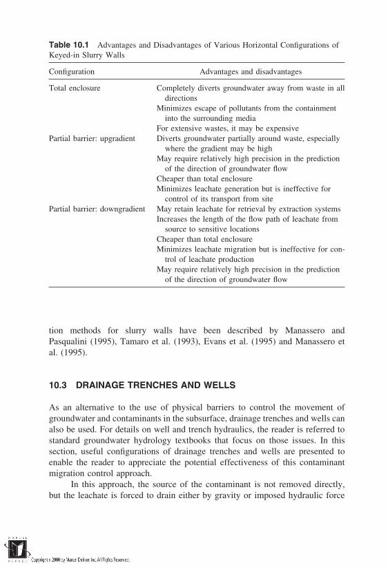
Table 10.1 Advantages and Disadvantages of Various Horizontal Configurations ofKeyed-in Slurry Walls

Configuration Advantages and disadvantages

Total enclosure Completely diverts groundwater away from waste in alldirections

Minimizes escape of pollutants from the containmentinto the surrounding media

For extensive wastes, it may be expensivePartial barrier: upgradient Diverts groundwater partially around waste, especially

where the gradient may be highMay require relatively high precision in the prediction

of the direction of groundwater flowCheaper than total enclosureMinimizes leachate generation but is ineffective for

control of its transport from sitePartial barrier: downgradient May retain leachate for retrieval by extraction systems

Increases the length of the flow path of leachate fromsource to sensitive locations

Cheaper than total enclosureMinimizes leachate migration but is ineffective for con-

trol of leachate productionMay require relatively high precision in the prediction

of the direction of groundwater flow

tion methods for slurry walls have been described by Manassero andPasqualini (1995), Tamaro et al. (1993), Evans et al. (1995) and Manassero etal. (1995).

10.3 DRAINAGE TRENCHES AND WELLS

As an alternative to the use of physical barriers to control the movement ofgroundwater and contaminants in the subsurface, drainage trenches and wells canalso be used. For details on well and trench hydraulics, the reader is referred tostandard groundwater hydrology textbooks that focus on those issues. In thissection, useful configurations of drainage trenches and wells are presented toenable the reader to appreciate the potential effectiveness of this contaminantmigration control approach.

In this approach, the source of the contaminant is not removed directly,but the leachate is forced to drain either by gravity or imposed hydraulic force

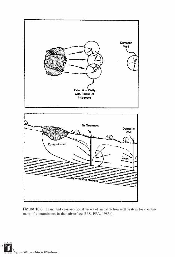
Figure 10.8 Plane and cross-sectional views of an extraction well system for contain-ment of contaminants in the subsurface (U.S. EPA, 1985c).

Figure 10.9 Use of a subsurface trench for containment of a contaminant plume (U.S.EPA, 1985c).

to a trench or wells from which it is removed by pumping. Thus, this method ofcontainment requires the use of above-ground treatment systems. Injection wellsmay be used to flush the contaminant source and increase the hydraulic potentialfor migration of contaminated water to extraction wells or trenches. As illustratedin Figures 10.8 and 10.9, each well has its radius of influence. Their spacingshould be such that their zones of influence overlap to promote effective contain-ment. A system of collector pipes can also be used with a main collector pipeas illustrated in Figure 10.10 to enhance areal coverage and the effectiveness ofthe plume containment.

Figure 10.10 Configuration of collector pipes and the main discharge pipe for extrac-tion of contaminated groundwater (adapted from U.S. EPA, 1985c).

10.4 SURFACE IMPOUNDMENTS

Surface impoundments are natural or man-made topographic depressions or dikedareas, bounded primarily by earthen materials and other engineered materials,and designed to hold liquid wastes or other wastes that contain free liquids. Im-poundments are often lined with clay, polymeric materials, or both. Examplesof surface impoundments are lagoons, settling and storage pits, and ponds. Con-crete-lined basins are not ordinarily classified as impoundments. Impoundmentsmay range in size from a few square meters to a few hundred acres. They canbe made to extend below the ground surface as in Figure 10.11A, or they canbe created on the ground surface through a system of well-configured dikes asshown in Figure 10.11B.

Surface impoundments may be temporary or permanent. Typically, they

A

B

Figure 10.11 A. An entrenched surface impoundment. B. A surface impoundment thatincorporates a dike.

serve as open containments for waste waters and sludges exuded from treatmentprocesses.

Temporary impoundment. Wastes are usually removed and the sites treatedafter closure of a temporary impoundment. A single liner, made of natu-ral or synthetic materials, is specified. The unit is designed to preventbreakthrough during the life of the impoundment.

Permanent surface impoundments. Permanent impoundments are usuallyclosed after their active lives. Before closure, the liquid fraction of thewaste must be removed and the solids stabilized.

10.5 GROUT CURTAINS

Grout curtains are barriers that are formed by pumping pore-filling materials intothe ground, thereby reducing the rate at which fluids can subsequently travelthrough the ground. Typically, the grout mixture is injected under pressure,

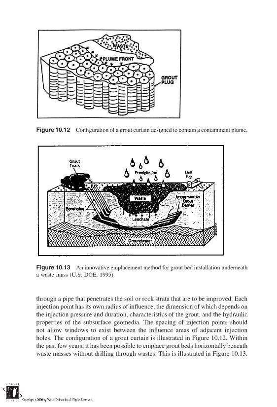
Figure 10.12 Configuration of a grout curtain designed to contain a contaminant plume.

Figure 10.13 An innovative emplacement method for grout bed installation underneatha waste mass (U.S. DOE, 1995).

through a pipe that penetrates the soil or rock strata that are to be improved. Eachinjection point has its own radius of influence, the dimension of which depends onthe injection pressure and duration, characteristics of the grout, and the hydraulicproperties of the subsurface geomedia. The spacing of injection points shouldnot allow windows to exist between the influence areas of adjacent injectionholes. The configuration of a grout curtain is illustrated in Figure 10.12. Withinthe past few years, it has been possible to emplace grout beds horizontally beneathwaste masses without drilling through wastes. This is illustrated in Figure 10.13.

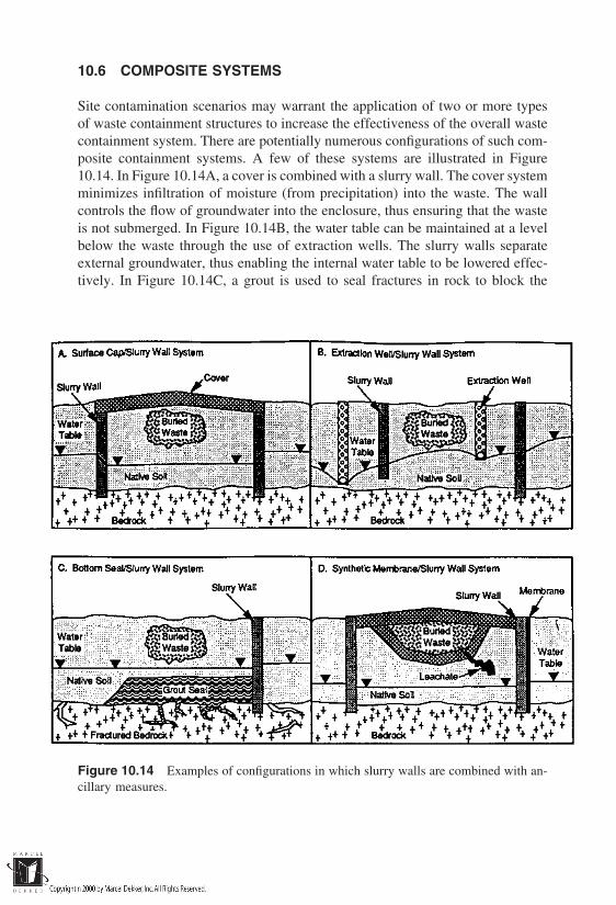
10.6 COMPOSITE SYSTEMS

Site contamination scenarios may warrant the application of two or more typesof waste containment structures to increase the effectiveness of the overall wastecontainment system. There are potentially numerous configurations of such com-posite containment systems. A few of these systems are illustrated in Figure10.14. In Figure 10.14A, a cover is combined with a slurry wall. The cover systemminimizes infiltration of moisture (from precipitation) into the waste. The wallcontrols the flow of groundwater into the enclosure, thus ensuring that the wasteis not submerged. In Figure 10.14B, the water table can be maintained at a levelbelow the waste through the use of extraction wells. The slurry walls separateexternal groundwater, thus enabling the internal water table to be lowered effec-tively. In Figure 10.14C, a grout is used to seal fractures in rock to block the

Figure 10.14 Examples of configurations in which slurry walls are combined with an-cillary measures.

contamination of the fractures and subsequent feedback of contaminants togroundwater. The slurry wall isolates external groundwater from the potentiallycontaminated zone. In Figure 10.14D, the use of a slurry wall to control possiblegroundwater contamination by releases from a landfill is illustrated. The externalsurface of a section of the slurry wall is covered by a geomembrane which pro-vides additional effectiveness against gas migration.

REFERENCES

Bass, J. M., Ehrenfeld, J. R., and Valentine, J. R. (1984). Potential Clogging of LandfillDrainage Systems. EPA-600/S2-83-1090. U.S. Environmental Protection Agency,Municipal Environmental Research Lab., Cincinnati, OH.

Benson, C. H., and Othman, M. A. (1993). Hydraulic conductivity of compacted clayfrozen and thawed in-situ. J. Geotech. Eng. 19(2):276–294.

Bonaparte, R. 1995. Long-term performance of landfills. Proc. ASCE Geoenvironment2000 Conf., New Orleans, LA, pp. 514–553.

Cope, F. W. (1987). Design of waste containment structures. Proc. Specialty Conf.Geotechnical Practice for Waste Disposal, Ann Arbor, MI, pp. 1–20.

Cosler, D. J., and Snow, R. E. (1984). Leachate collection system performance analyses.J. Geotech. Eng. vol. 110(8):1024–1041.

Duplancic, N. 1987. Hazardous waste landfill cap system stability. Proc. Specialty Conf.on Geotechnical Practice for Waste Disposal, Ann Arbor, MI, pp. 432–446.

Duvel, W. A. (1979). Solid waste disposal: Landfilling. Chem. Eng. 86(14):77–86.Emcon Associates. (1982). Field Assessment of Site Closure, Boone County, Kentucky.

U.S. Environmental Protection Agency, Cincinnati, OH.Evans, J. C., Costa, M. J., and Cooley, B. (1995). The state of stress in soil-bentonite

slurry trench cut off walls. Proc. ASCE Geoenvironment 2000 Conf., New Orleans,LA, pp. 1173–1191.

Giroud, J. P., and Ah-Line, C. (1984). Design of earth and concrete covers for geomem-branes. Proc. Int. Conf. on Geomembranes, Denver, CO, pp. 487–492.

Glebs, R. T. (1980). Under right conditions, landfills can extend below ground water table.Solid Waste Management, 23(2):50–59.

Goodall, D. C., and Quigley, R. M. (1977). Pollutant migration from two sanitary landfillsites near Sarnia, Ontario. Can. Geotech. J. 14(2):223–236.

Gordon, M. E., and Huebner, P. M. (1983). An evaluation of the performance of zone ofsaturation landfills in Wisconsin. Proc. 6th Annual Madison Conf. of Applied Re-search and Practice on Municipal and Industrial Waste, University of Wisconsin,Madison.

Haikola, B. M., Loehr, R. C., and Daniel, D. E. (1995). Hazardous waste landfill perfor-mance as measured by primary leachate quantity. Proc. ASCE Geoenvironment2000 Conf., New Orleans, LA, pp. 554–567.

Haxo, H. E. (1980). Interaction of selected liner materials with various hazardous wastes.In Disposal of Hazardous Wastes, Proc. 6th Annual Research Symp., EPA-600/9-80-010. U.S. Environmental Protection Agency, Cincinnati, OH, pp. 160–180.

Hughes, J. (1975). Use of bentonite as a soil sealant for leachate, control in sanitary land-fills. Soil Lab. Report 280-E, American Colloid Co., Skokie, IL.

Inyang, H. I. (1992). Selection and design of slurry walls as barriers to control pollutantmigration. Draft Technical Guidance Document, Office of Solid Waste and Emer-gency Response, U.S. Environmental Protection Agency, Washington, DC.

Inyang, H. I. (1994). A Weibull-based reliability analysis of waste containment systems.Proc. First Int. Congress on Environmental Geotechnics, Alberta, Canada, pp. 273–278.

Inyang, H. I., Fang, H. Y., Iskandar, A., and Choquette, M. R. (1997a). Chemical andmineralogical analyses of clayey barrier materials. Encyclopedia of EnvironmentalAnalysis and Remediation, Vol. 8, pp. 5131–5141. Wiley, New York.

Inyang, H. I., Iskandar, A., and Parikh, J. M. (1997). Physico-chemical interactions inwaste containment barriers. In. Encyclopedia of Environmental Analysis and Reme-diation, Vol. 2, pp. 1158–1165. Wiley, New York.

Inyang, H. I., and Tumay, M. T. (1995). Containment systems for contaminants in thesubsurface. In Encyclopedia of Environmental Control Technology, pp. 175–215.Gulf Publishing Company.

Koerner, R. M. (1990). Designing with Geosynthetics, 2nd ed. Prentice-Hall.Koerner, R. M., and Whitty, J. E. (1984). Experimental friction evaluation of slippage

between geomembranes, geotextiles, and soils. Proc. Int. Conf. on Geomembranes,Denver, CO, pp. 191–196.

Manassero, M., Fratalocchi, E., Pasqualine, E., Spanna, C., and Verga, F (1995). Contain-ment with vertical cut off walls. Proc. ASCE Geoenvironment 2000 Conf., NewOrleans, LA, pp. 1142–1172.

Manassero, M., and Pasqualini, E. (1992). Ground pollutant containment barriers. Proc.Mediterranean Conf. on Environmental Geotechnology, Cesme, Turkey, pp. 195–204.

Quinn, K. J. (1983). Numerical simulation of zone of saturation landfill designs. Proc.6th Annual Madison conf. on Applied Research and Practice on Municipal andIndustrial Waste, University of Wisconsin, Madison.

Reid, G., Streebin, L. E., Canter, L. W., Robertson, J. M., and Klehro, E. (1971). Develop-ment of specification for liner materials for use in oil-brine pits, lagoons, and otherretention systems. Draft, Oklahoma Economic Development Foundation, Norman,OK.

Richardson, G. N., and Koerner, R. M. (1989). Geosynthetic Design Guidance for Hazard-ous Waste Landfill Cells and Surface Impoundments. Geosynthetic Research Insti-tute, Drexel University, Philadelphia.

Tamaro, M., Pamukai, S., and Lopez, P. (1993). Prediction of structural slurry wall behav-ior. Proc. Third Int. Conf. on Case Histories in Geotechnical Engineering, St.Louis, MO, pp. 695–701.

Thornton, D. E., and Blackwell, P. (1976). Field Evaluation of Plastic Film Liners forPetroleum Storage Area in the McKenzie Delta. EPS-3-EC-76-13. Canadian Envi-ronmental Protection Service, Edmonton, Alberta.

U.S. DOE. (1995). Landfill Stabilization Focus Area. Technology Summary DOE/EM-0251. Office of Environmental Management and Technology Development, U.S.Department of Energy, Washington, DC.

U.S. EPA. (1991). Design and Construction of RCRA/CERCLA Final Covers. EPA/625/4-91/025. Office of Research and Development, U.S. Environmental ProtectionAgency, Washington, DC.

U.S. EPA. (1989). Requirement for Hazardous Waste Landfill Design, Construction andClosure. Seminar Publication. EPA/625/4-89/022. Office of Research and Devel-opment, U.S. Environmental Protection Agency, Washington, DC.

U.S. EPA. (1985a). Draft. Minimum Technology Guidance Document on Double LinerSystems for Landfills and Surface Impounds: Design, Construction, and Operation.U.S. Environmental Protection Agency, Washington, DC.

U.S. EPA. (1985b). Minimum Technology Guidance on Single Liner Systems for Land-fills, Surface Impoundments, and Waste Piles—Design, Construction, and Opera-tion. Draft. EPA/530-SW-85-013. U.S. Environmental Protection Agency, Wash-ington, D.C.

U.S. EPA. (1985c). Leachate Plume Management. Publication EPA/540/2-85/004. Officeof Emergency and Remedial Response, U.S. Environmental Protection Agency,Washington, DC.

Ware, S., and Jackson, G. (1978). Liners for Sanitary Landfills and Chemical HazardousWaste Disposal Sites. EPA-600/9-78-005. U.S. Environmental Protection Agency,Cincinnati, OH.

Weston, R. F. Inc. (1989). Pollution Prediction Techniques for Waste Disposal Siting: AState-of-the-Art Assessment. EPA-SW-162C. U.S. Environmental ProtectionAgency, Cincinnati, OH.

11Elements of ContainmentSystem Design

11.1 INTRODUCTION

A waste containment system is expected to perform two important functions: (1)it should prevent or minimize transport of contaminants from within itself to thesurrounding soil and groundwater, and (2) it should retain its structural integrityduring the design life period. The first function requires the application of masstransfer and transport principles (discussed in Chapter 4), whereas the secondfunction requires the application of geotechnical aspects, primarily slope stabilityand settlement principles. These two functions are central not only to the overallsiting and design of containment systems but also to the design of individualcomponents such as top covers, bottom liners, drainage systems, slurry walls,etc. To fulfill the first function, we need to address the following questions:

1. What is the rate of infiltration into the waste material?2. What proportion of the infiltrated water may be expected to cross the

barrier?3. What is the quality of the liquid that exits the barriers?

Fulfillment of the second function involves estimation of factor of safetyagainst slope failure of the containment system, and settlement calculations. Withthe increased use of polymeric materials in barriers, this also involves checkingfor the stability of interfaces between geomembranes and soils.

We will take up these two functions in this chapter from system scale tocomponent scale. Thus, we will look first at the water balance of the system,before discussing flow and transport through the barrier layers. In the discussionof stability issues, we will summarize the essential principles of slope stabilityand settlement analyses that are pertinent to waste containment systems. For adetailed discussion of these issues, the reader is advised to consult a standardtextbook on geotechnical engineering.

11.2 LEACHATE GENERATION

As water from rainfall or runoff infiltrates into a waste containment system, itreacts with the solid and liquid constituents of the waste. During the percolationprocess, the infiltrating water is usually contaminated by the waste. Dependingon the type of waste and the reactions between the percolating water and thewaste, this percolated water, commonly termed leachate, may become highlycontaminated. The most common reaction processes occurring within the wasteare (1) dissolution of certain solid forms of the waste and subsequent precipita-tion; (2) decomposition and disintegration of the solids; and (3) reactions betweenthe original liquids contained in the waste and the percolating water. The concen-trations of various chemicals in the leachate are governed by a number of masstransfer processes operating simultaneously. For instance, an acidic pH conditionof the liquid may trigger a number of processes, such as dissolution and precipita-tion, ion exchange, and sorption, simultaneously, as discussed in Chapter 4.

Apart from the reaction processes occurring within the waste, the concen-trations of the leachate produced also depend on the waste disposal technique

Table 11.1 Ranges of Constituent Concentrations (in mg/L Unless Noted) inLeachate from Municipal Waste Landfills (EPA/530-SW-86-054, 1986)

Concentration ConcentrationConstituent range Constituent range

COD 50–90,000 Hardness (as CaCO3) 0.1–36,000BOD 5–75,000 Total P 0.1–150Total organic carbon (TOC) 50–45,000 Organic P 0.4–100Total solids (TS) 1–75,000 Nitrate nitrogen 0.1–45TDS 725–55,000 Phosphate (inorganic) 0.4–150Total suspended solids (TSS) 10–45,000 Ammonia nitrogen (NH3-N) 0.1–2,000Volatile suspended solids (VSS) 20–750 Organic N 0.1–1,000Total volatile solids (TVS) 90–50,000 Total Kjeldahl nitrogen (TKN) 7–1,970Fixed solids (FS) 800–50,000 Acidity 2,700–6,000AlKalinity (as CaCO3) 0.1–20,350 Turbidity (Jackson units) 30–450Total coliform (CFU/100 mL) 0–105 Cl 30–5,000Fe 200–5,500 PH (dimensionless) 3.5–8.5Zn 0.6–220 Na 20–7,600Sulfate 25–500 Cu 0.1–9Ni 0.2–79 Pb 0.001–1.44Total volatile acids (TVA) 70–27,700 Mg 3–15,600Mn 0.6–41 K 35–2,300Fecal coliform (CFU/1,000 ml) 0–105 Cd 0–0.375Specific conductance (mhg/cm) 960–16,300 Hg 0–0.16Ammonium nitrogen (NH4-N) 0–1,106 Se 0–2.7

Cr 0.02–18

Table 11.2 Representative Hazardous Substances within Industrial Waste Streams

Hazardous substances

Chlorinated Misc.Industry Arsenic Cadmium hydrocarbonsa Chromium Copper Cyanides Lead Mercury organicsb Selenium Zinc

Battery

Chemical manufacturing

Electrical and electronic

Electroplating and metal

finishingExplosives

Leather

Mining and metallurgy

Paint and dye

Pesticide

Petroleum and coal

Pharmaceutical

Printing and duplicating

Pulp and paper

Textile

a Including polychlorinated biphenyls.b For example, acrolein, chloropicrin, dimethyl sulfate, dinitrobenzene, dinitrophenol, nitroaniline, and pentachlorophenol.Source: Matrecon, Inc. (1980).

and time elapsed after the waste disposal. In general, the concentrations of chemi-cals in leachate are believed to reach a peak value some time after the placementof waste, and then decrease with time. This decrease in concentrations with timeis due to dilution, biochemical processes leading to breakdown of chemicals, andcontinuous removal of leachate from a collection point (Rowe, 1991; Ehrig andScheelhaase, 1993; Lu et al., 1985).

Because of these various factors, leachate quality in a containment systemusually exhibits tremendous spatial and temporal variability. A knowledge of thepredominant constituents in the leachate is essential in order to design the wastecontainment barriers. Table 11.1 shows the typical ranges of constituent concen-trations found in leachate from municipal waste landfills. In contrast to municipalwaste landfills, hazardous waste landfills typically contain elevated amounts ofheavy metals, organic compounds, and other toxic substances. Table 11.2 showsrepresentative hazardous constituents that may be expected in industrial leachate.

To assess the impact of leachate generation on the quality of soil andgroundwater in the vicinity, one needs to estimate both the quantity and the qual-ity of leachate exiting the containment system. In the next three sections, we willdiscuss methods commonly adopted to estimate leachate quantity and quality.

11.3 WATER BALANCE IN WASTE CONTAINMENTSYSTEMS

The total quantity of leachate generated at a given waste containment system isprimarily a function of the quantity of water infiltrated into the system and quan-tity of fluids generated within the waste. The former is in turn dependent on anumber and intensity of climatologic and hydrologic processes, primarily rainfall,runoff, and evaporation. Thus, to estimate the quantity of leachate, one needs toconduct a water balance for the entire system. This essentially involves a bookkeep-ing procedure to account for the final disposition of total precipitation at a givensite, through a number of pathways such as evaporation, infiltration, and runoff.

Figure 11.1 shows the various pathways through which precipitation at awaste containment system is disposed of. Precipitation in the form of snow orrainfall is partitioned into interception by vegetation (for subsequent evapotrans-piration), temporary storage followed by subsequent runoff from the surface ofthe system, and infiltration into the cover. The proportion of the precipitationthat infiltrates into the system will alter the water storage in the topsoil, whichwill undergo possible evapotranspiration from the vegetation and the soils. Inaddition, a proportion of the infiltrated water may be carried through a lateraldrainage system if one is provided in the surface cover system. Eventually, aportion of the infiltrated water may travel down into the waste, past the topsoilcover and barrier, and contribute to leachate percolation.

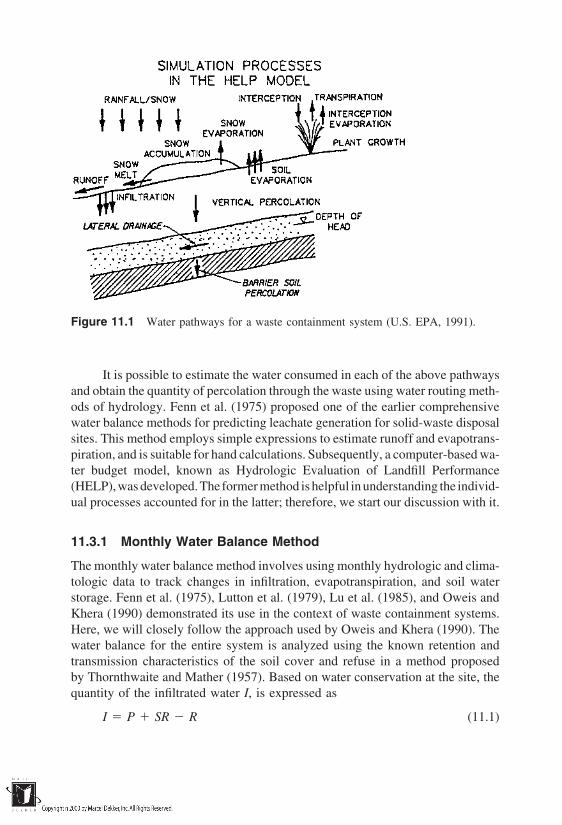
Figure 11.1 Water pathways for a waste containment system (U.S. EPA, 1991).

It is possible to estimate the water consumed in each of the above pathwaysand obtain the quantity of percolation through the waste using water routing meth-ods of hydrology. Fenn et al. (1975) proposed one of the earlier comprehensivewater balance methods for predicting leachate generation for solid-waste disposalsites. This method employs simple expressions to estimate runoff and evapotrans-piration, and is suitable for hand calculations. Subsequently, a computer-based wa-ter budget model, known as Hydrologic Evaluation of Landfill Performance(HELP), was developed. The former method is helpful in understanding the individ-ual processes accounted for in the latter; therefore, we start our discussion with it.

11.3.1 Monthly Water Balance Method

The monthly water balance method involves using monthly hydrologic and clima-tologic data to track changes in infiltration, evapotranspiration, and soil waterstorage. Fenn et al. (1975), Lutton et al. (1979), Lu et al. (1985), and Oweis andKhera (1990) demonstrated its use in the context of waste containment systems.Here, we will closely follow the approach used by Oweis and Khera (1990). Thewater balance for the entire system is analyzed using the known retention andtransmission characteristics of the soil cover and refuse in a method proposedby Thornthwaite and Mather (1957). Based on water conservation at the site, thequantity of the infiltrated water I, is expressed as

I P SR R (11.1)

where P precipitation, SR water carried by surface runoff into the system,and R surface runoff out of the system. The pathway of interception by vegeta-tion is ignored in Eq. (11.1). R may be estimated by any of the empirical methodsavailable in the hydrology literature. Rational formula offers a simple way ofestimating R as a proportion of precipitation. That is,

R CP (11.2)

where C runoff coefficient, which is a function of soil type, vegetation, andsurface topography. Table 11.3 shows typical values of C. Once the quantity ofinfiltrated water I is known via Eq. (11.1), the quantity percolated out of the soilcover into the waste can be estimated applying water conservation principles tothe soil cover. Thus,

PER I AET ∆Sc (11.3)

where PER quantity of water percolated out of the soil cover, AET actualevapotranspiration from the cover, and ∆Sc change in storage of the cover asa result of infiltration. We make a distinction here between the potential evapo-transpiration (PET ) and actual evapotranspiration (AET ). PET occurs when morethan adequate moisture is available to meet the evaporative demand of the atmo-sphere. AET, on the other hand, is the actual amount of evapotranspiration thattakes place when the soil is dry (I PET ), therefore the evaporation demandcannot be met. Thus, AET is always less than or equal to PET.

The monthly potential evapotranspiration may be estimated using theThornthwaite equation,

PET (mm) 1610t

TEa

(11.4)

Table 11.3 Runoff Coefficients as Affected by Cover Material and Slope

Runoff coefficient, C

Flat: Rolling: Hilly:Type of area slope 2% slope 2–10% slope 10%

Grassed areas 0.25 0.3 0.3Earth areas 0.6 0.65 0.7Meadows and pasture lands 0.25 0.3 0.35Cultivated land:

Impermeable (clay) 0.5 0.55 0.6Permeable (loam) 0.25 0.3 0.35

Source: Perry (1976).

where t temperature of the month under consideration, and TE temperatureefficiency index, given as the summation of the heat indices of the 12 monthsin the year. Considering that heat index for a given month is expressed as (t/5)1.514, TE may be written as

TE 12

i1ti

51.514

(11.5)

In Eq. (11.4), a is an empirical coefficient given by

a 6.75 107(TE )3 7.7 105(TE )2

(11.6) 1.79 102(TE ) 0.492 39

PET, as given by Eq. (11.4), also depends on the hours of sunlight, in additionto the temperature and the heat index. To account for the unequal durations ofsunlight (daylight times) during the year, PET is usually multiplied by an adjust-ment factor. Values of this factor, listed in Table 11.4, depend on the month ofthe year and latitude of the location under consideration.

Equation (11.3) is implemented as follows to determine the percolationquantities. The quantity (I PET ) is first calculated. If this quantity is positive,the evaporative demand by the atmosphere is met, and the surplus goes downinto the soil cover and makes it wetter. In this case, AET PET. If the watercontent of the soil cover is already high—say, at its field capacity—the soil canstore no additional water and the surplus will percolate into the waste (note thatthe field capacity is the maximum water content that a soil can retain under gravi-tational draining). On the other hand, if (I PET ) is negative, the evaporationdemand by the atmosphere is not met, and AET PET. The soil gives up itswater content to the atmosphere, if it is wet, and gets dryer. The amount of dryingdepends not only on the magnitude of (I PET ), but also on the water contentof the soil cover. Under these conditions, no percolation occurs until there arisesa situation when (I PET ) is again positive and the topsoil cover is brought toits field capacity.

The amount of drying from the soil cover that takes place during the dryspell (when there is no percolation) depends on the type of soil and the cumula-tive water deficit. This is essentially a problem of flow through unsaturatedsoil. Thornthwaite and Mather (1957) provide tables with which one can esti-mate the soil moisture retention after evapotranspiration occurred from a drysoil. Table 11.5 provides an abbreviated form as documented in Oweis andKhera (1990). The soil moisture storage required in this table may be obtainedfrom Fig. 11.2, which summarizes the water-holding characteristics of varioussoils.

Table 11.4 Adjustment Factors for Potential Evapotranspiration Computed by the Thornthwaite Equation

Latitude Jan. Feb. Mar. Apr. May June July Aug. Sep. Oct. Nov. Dec.

0 1.04 0.94 1.04 1.01 1.04 1.01 1.04 1.04 1.01 1.04 1.01 1.0410 1.00 0.91 1.03 1.03 1.08 1.06 1.08 1.07 1.02 1.02 0.98 0.9920 0.95 0.90 1.03 1.05 1.13 1.11 1.14 1.11 1.02 1.00 0.93 0.9430 0.90 0.87 1.03 1.08 1.18 1.17 1.20 1.14 1.03 0.98 0.89 0.8835 0.87 0.85 1.03 1.09 1.21 1.21 1.23 1.16 1.03 0.97 0.86 0.8540 0.84 0.83 1.03 1.11 1.24 1.25 1.27 1.18 1.04 0.96 0.83 0.8145 0.80 0.81 1.02 1.13 1.28 1.29 1.31 1.21 1.04 0.94 0.79 0.7550 0.74 0.78 1.02 1.15 1.33 1.36 1.37 1.25 1.06 0.92 0.76 0.70

Source: Chow (1964).

Table 11.5 Soil Moisture Retention After Potential Evapotranspiration Has Occurred

Sr (mm)b

∑NEG(I-PET )a 25 50 75 100 125 150 200 250 300

0 25 50 75 100 125 150 200 250 30010 16 41 65 90 115 140 190 240 29020 10 33 57 81 106 131 181 231 28030 7 27 50 74 98 122 172 222 27140 4 21 43 66 90 114 163 213 26250 3 17 38 60 83 107 155 204 25460 2 14 33 54 76 100 148 196 24570 1 11 28 49 70 93 140 188 23780 1 9 25 44 65 87 133 181 22990 1 7 22 40 60 82 127 174 222100 6 19 36 55 76 120 167 214150 2 10 22 37 54 94 136 181200 1 5 13 24 39 73 111 153250 2 8 16 28 56 91 130300 1 5 11 20 44 74 109350 1 3 7 14 34 61 92400 2 5 10 26 50 78450 1 3 7 20 41 66500 1 2 5 16 33 56600 1 3 10 22 40700 1 6 15 28800 1 4 10 201000 1 4 10

a NEG(I-PET) is lack of infiltration water needed for vegetation.b Sr, soil moisture storage at field capacity.Source: Oweis and Khera (1990).

The final estimate of leachate, q, coming out of the refuse, may now beobtained by applying water conservation principle to the waste body. Thus,

q PER Wd ∆Sw (11.7)

where Wd water generated from waste decomposition, and ∆Sw change inmoisture storage of the waste. Until the waste attains its field capacity, no leachatemay be expected at its bottom. The percolation will first satisfy the moisture-holding capacity of the waste and the surplus will then leach out of the waste.The water-holding capacity of waste is highly variable, as shown in Table 11.6for some common types of refuse. Depending on the permeability of the barrier

Figure 11.2 Water storage capacities of USDA soils (Lutton et al. 1979).

at the bottom of the refuse, a leachate mound may form, which provides a hydrau-lic head for leakage through the barrier.

As discussed in the preceding paragraphs, the monthly water balancemethod requires accounting of how the precipitation is apportioned, one monthat a time. The simple expressions involved in the calculations make it suitablefor spreadsheet programming. Detailed case studies using this method are givenby Fenn et al. (1975), Lutton et al. (1979), Lu et al. (1985), and Oweis and Khera(1990).

11.3.2 Hydrologic Evaluation of Landfill Performance(HELP)

Hydrologic Evaluation of Landfill Performance (HELP) is a computer programdeveloped by the U.S. Army Waterways Experiment Station, which was designedfor water budget modeling of waste containment systems. Details of the programimplementation, applications, and its limitations are provided by Schroeder et al.(1984a, 1984b) and the U.S. EPA (1991). Only an outline of this method is pro-vided here, in order to highlight the important factors affecting leachate quantityestimates. The program has become popular during recent years primarily be-

Table 11.6 Water Absorption Ranges for Solid Waste Components

Moisture content, percent dry weight

Total moisture-holdingWater absorption capability capabilitya

Component Maximum Average Minimum Maximum Average Minimum

Newsprintb 290 290c

Cardboard (solid and cor- 170 170c

rugated)b

Other miscellaneous paper 400 100 400c 100c

Lawn clippings (grass and 200 60 370 140leaves)

Shrubbery, tree prunings 100 10 250 10Food waste (kitchen gar- 100 0 300 0

bage)Textiles (cloth of all 300 100 300c 100c

types, rope)Wood, plastic, glass, 0 0

metal (all inorganic)

a Calculated from water absorption plus initial moisture content in as-received samples.b Sample variation was negligible.c Initial moisture contents as-received were less than 6% in the laboratory tests; therefore, they were

considered negligible compared to the variation in moisture absorbed.Source: Stone (1974).

cause of its ability to incorporate a number of layers in a waste containmentsystem and also to account for the lateral drainage in individual layers. Besidesproviding accurate estimates of water budget components, HELP is useful inevaluating and comparing alternative containment systems.

A typical hazardous-waste containment profile that HELP is capable ofsimulating is shown in Figure 11.3. The model uses methods similar to thosedescribed in the previous section. It apportions the precipitation into severalwater budget components as the water percolates through each of the layers.These components include not only surface runoff, evapotranspiration, and watercontent changes in the soils, but also the lateral drainage collected in eachdrain system, and percolation through each layer of the system. It can generatedaily, monthly, annual, and long-term average water budgets. A number ofphysical and hydrologic methods are used in HELP to simulate individual waterbudget components. A short summary of these methods is given below. Priorunderstanding of these methods is essential to interpret the simulation resultscorrectly.

Figure 11.3 Waste containment profile that can be simulated in HELP (U.S. EPA,1991).

Infiltration

Infiltration is estimated indirectly by subtracting the runoff and surface evapo-transpiration from rainfall and snowmelt. Runoff and surface evapotranspirationare treated as functions of interception. Snowmelt is computed using a modifiedversion of the simple degree-day method with 0°C as the base temperature(USDA, 1972). Interception is modeled after the work of Horton (1919). It ap-proaches a maximum value exponentially as the rainfall increases to about 0.5

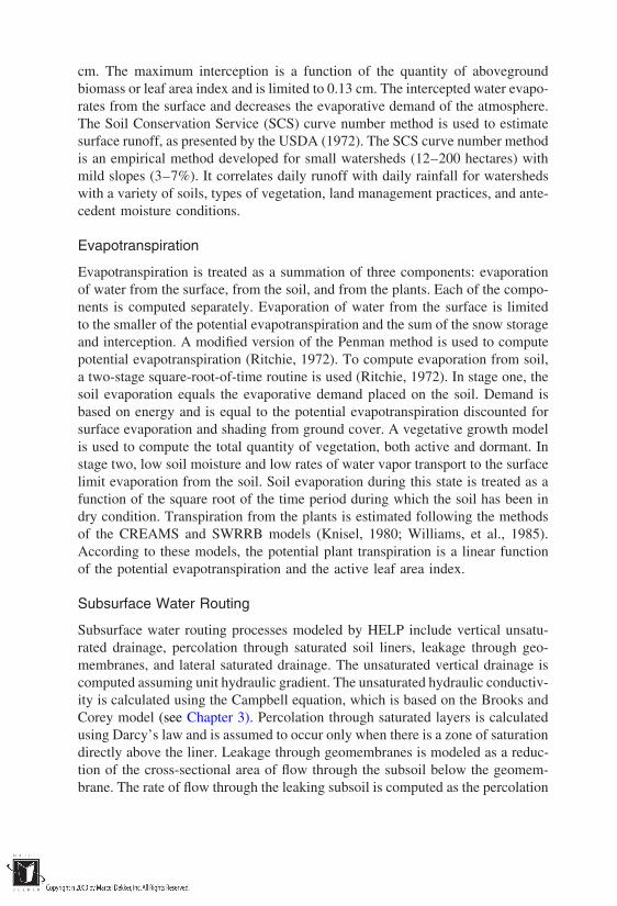
cm. The maximum interception is a function of the quantity of abovegroundbiomass or leaf area index and is limited to 0.13 cm. The intercepted water evapo-rates from the surface and decreases the evaporative demand of the atmosphere.The Soil Conservation Service (SCS) curve number method is used to estimatesurface runoff, as presented by the USDA (1972). The SCS curve number methodis an empirical method developed for small watersheds (12–200 hectares) withmild slopes (3–7%). It correlates daily runoff with daily rainfall for watershedswith a variety of soils, types of vegetation, land management practices, and ante-cedent moisture conditions.

Evapotranspiration

Evapotranspiration is treated as a summation of three components: evaporationof water from the surface, from the soil, and from the plants. Each of the compo-nents is computed separately. Evaporation of water from the surface is limitedto the smaller of the potential evapotranspiration and the sum of the snow storageand interception. A modified version of the Penman method is used to computepotential evapotranspiration (Ritchie, 1972). To compute evaporation from soil,a two-stage square-root-of-time routine is used (Ritchie, 1972). In stage one, thesoil evaporation equals the evaporative demand placed on the soil. Demand isbased on energy and is equal to the potential evapotranspiration discounted forsurface evaporation and shading from ground cover. A vegetative growth modelis used to compute the total quantity of vegetation, both active and dormant. Instage two, low soil moisture and low rates of water vapor transport to the surfacelimit evaporation from the soil. Soil evaporation during this state is treated as afunction of the square root of the time period during which the soil has been indry condition. Transpiration from the plants is estimated following the methodsof the CREAMS and SWRRB models (Knisel, 1980; Williams, et al., 1985).According to these models, the potential plant transpiration is a linear functionof the potential evapotranspiration and the active leaf area index.

Subsurface Water Routing

Subsurface water routing processes modeled by HELP include vertical unsatu-rated drainage, percolation through saturated soil liners, leakage through geo-membranes, and lateral saturated drainage. The unsaturated vertical drainage iscomputed assuming unit hydraulic gradient. The unsaturated hydraulic conductiv-ity is calculated using the Campbell equation, which is based on the Brooks andCorey model (see Chapter 3). Percolation through saturated layers is calculatedusing Darcy’s law and is assumed to occur only when there is a zone of saturationdirectly above the liner. Leakage through geomembranes is modeled as a reduc-tion of the cross-sectional area of flow through the subsoil below the geomem-brane. The rate of flow through the leaking subsoil is computed as the percolation

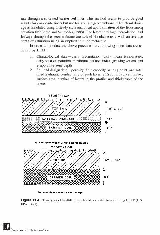
rate through a saturated barrier soil liner. This method seems to provide goodresults for composite liners but not for a single geomembrane. The lateral drain-age is simulated using a steady-state analytical approximation of the Boussinesqequation (McEnroe and Schroeder, 1988). The lateral drainage, percolation, andleakage through the geomembrane are solved simultaneously with an averagedepth of saturation using an implicit solution technique.

In order to simulate the above processes, the following input data are re-quired by HELP:

1. Climatological data—daily precipitation, daily mean temperature,daily solar evaporation, maximum leaf area index, growing season, andevaporative zone depth

2. Soil and design data—porosity, field capacity, wilting point, and satu-rated hydraulic conductivity of each layer, SCS runoff curve number,surface area, number of layers in the profile, and thicknesses of thelayers

Figure 11.4 Two types of landfill covers tested for water balance using HELP (U.S.EPA, 1991).

The program includes default daily weather data for 102 U.S. cities and iscapable of synthetically generating weather data for 183 U.S. cities. In addition,default data are included for 15 soil types as well as solid waste. Default SCScurve numbers are also provided. The output from the HELP consists primarilyof percolation or leakage through each layer and depth of saturation on the surfaceof liners. Incremental and cumulative qualities of water budget for the variouscomponents are also provided.

The HELP model allows one to look at the sensitivity of the water balanceto various design variables. Case studies were reported by the U.S. EPA (1991)demonstrating the sensitivity analyses. The climatologic regimes at three differentlocations (Santa Maria, CA; Schenectady, NY; and Shreveport, LA) were usedto study the water balance for two typical landfill covers (Fig. 11.4). Two typesof topsoils with different thicknesses were also studied. The results from thesimulations are shown in Tables 11.7–11.9. Table 11.7 shows the effects of cli-mate and vegetation with and without lateral drainage. It is seen that vegetationdecreases runoff and increases evapotranspiration but tends to have little effecton the rest of the water balance. A three-layer cover design (which allows forlateral drainage) is definitely superior to a two-layer design, indicating that thedesign of the cover is far more important than the climatologic and vegetationfactors. It should be noted that although vegetation is shown to have little effect

Table 11.7 Effects of Climate and Vegetation on Water Balance

Two-layer cover designa Three-layer cover designb

location location

CA LA NY CA LA NY(% precipitation) (% precipitation)

Poor grassRunoff 5.6 4.6 5.5 3.0 4.4 2.2Evapotranspiration 51.8 53.0 52.1 51.6 51.9 50.3Lateral drainage — — — 41.2 40.6 44.0Percolation 42.6 42.4 42.4 4.2 3.1 2.5

Good grassRunoff 3.1 0.2 3.5 0.0 0.2 0.0Evapotranspiration 55.0 57.2 55.3 52.6 53.0 51.0Lateral drainage — — — 43.2 43.7 45.5Percolation 42.9 42.6 41.2 4.2 3.1 2.5

a 900 mm of sandy loam topsoil and 0.6 m of 106 cm/s clay liner.b 450 mm of sandy loam topsoil, 300 mm of 0.03 cm/s sand with 60 m drain length at 3% slope,

and 0.6 m of 107 cm/s clay liner.Source: U.S. EPA (1991).

Table 11.8 Effects of Topsoil Thickness on Water Balance

45.7 cm of topsoil location 91.4 cm of topsoil location

CA LA NY CA LA NY(% precipitation) (% precipitation)

Runoff 11.2 7.5 13.4 5.6 4.6 5.5Evapotranspiration 51.9 56.9 54.5 51.8 53.0 52.1Percolation 36.9 35.6 32.1 42.6 42.4 42.4

Sandy loam topsoil with a poor stand of grass underlain by 0.6 m of 106 cm/s clay liner.Source: U.S. EPA (1991).

on percolation in these simulations, its importance lies elsewhere, in the contextof erosion prevention.

Table 11.8 shows the effects of topsoil thickness on the water balance forthe cover design where lateral drainage is absent. The effects of topsoil thicknessare similar for all three locations. Runoff and evapotranspiration were greater forthe thinner topsoil, indicating that the head above the barrier maintained highermoisture contents in the evaporative zone. The percolation was consequently lessthan for cases with greater topsoil thickness. Although thin topsoil is in generalfavorable for reduced percolation, it is important to provide adequate thicknessfor the top cover to support vegetation, maintain soil stability, and control erosion.

Table 11.9 shows the effects of topsoil type on water budget components.Clayey topsoil increased both runoff and evapotranspiration, which in turn greatlydecreased lateral drainage and percolation. Considering the California site, runoff

Table 11.9 Effects of Topsoil Type on Water Budget Components

Three-layer cover designa

Sandy loam location Silty clayey loam location

CA LA NY CA LA NY(% precipitation) (% precipitation)

Runoff 3.0 4.4 2.2 21.6 22.3 19.2Evapotranspiration 51.6 51.9 50.3 61.2 64.4 58.6Lateral drainage 41.2 40.6 44.0 15.0 11.3 20.3Percolation 4.2 3.1 2.5 2.2 2.0 1.9

a 450 mm of topsoil with poor stand of grass, 300 mm of 0.03 cm/s sand with 60 m drain length at3% slope, and 0.6 m of 107 cm/s clay liner.

Source: U.S. EPA (1991).

increased from 3% to 22% of the precipitation whereas evapotranspiration in-creased from 52% to 61% of precipitation, when the topsoil is changed fromsandy loam to a silty clayey loam. The lower hydraulic conductivity of clayeytopsoil slowed down the lateral drainage, which dropped from about 41% to 15%of precipitation. Because of these effects, percolation differed only slightly, from4% to 2%, between the two soil types.

11.4 LEACHATE COLLECTION AND REMOVAL SYSTEMS(LCRS)

Flow of leachate through barriers can be minimized in two ways—by minimizingthe leachate accumulated at the top of the barrier via a collection system, andby designing the barrier such that its permeability is very low. Design of theleachate collection system is an important element in the overall design of thewaste containment system. It includes sizing and spacing of the pipes used tocollect and remove the leachate. The total leachate percolated out of the wasteis apportioned between the leachate collection system and the liner leakage. Thusthe problem of leachate collection above the liner and that of flow through thebarrier is an integrated one and cannot be decoupled. In practice, however, sim-pler methods are used to predict the height of the leachate mound, assumingeither a constant leakage rate through the liner or no leakage at all. Leakagethrough the liner is often ignored for a conservative design of leachate collectionand treatment systems.

The maximum height of leachate mound above the barrier depends on howthe collection system is laid out. Figure 11.5 shows typical configurations forthe collection system. The configuration shown in Figure 11.5a offers a simpleexpression for maximum height, hmax, of the leachate mound. Applying Darcy’slaw to estimate flow in the drainage layer, the height of the mound, h(x), can beestimated as (see Table 3.5)

h(x) q

kd(L x)x

0.5

(11.8)

where q percolation rate of leachate coming onto the drainage layer, kd saturated hydraulic conductivity of the drainage layer, and L drain spacing.The maximum height of the mound occurs at the midpoint between the twodrains; therefore,

hmax L

2 q

kd

0.5

(11.9)

Figure 11.5 Leachate collection system configurations.

From a design standpoint, the drains must be capable of discharging (qL) perunit length, since the percolation over one-half of the drain spacing flows fromeither side of each drain. When one puts constraints on hmax, in order to ensurethat the mound lies totally within the drainage layer, Eq. (11.9) allows estimationof the required spacing L or hydraulic conductivity kd.

Figure 11.5b illustrates a more common configuration of a collection sys-tem, where the barriers are typically graded to enhance flow toward leachatecollection drains. Moore (1980) developed a solution for this case and expressedhmax as (see Table 3.5)

hmax L√c2 tan2 α

c 1

tan αc

√tan2 α c (11.10)

where c q/kd, and α slope angle of the liner. As stated earlier, Eq. (11.10)may also be used to obtain the required design parameters given hmax.

Other configurations for collections systems were also studied; for instance,McBean et al. (1982) considered a sloping collection system as in Figure 11.5bbut with drains at the apex of the barrier as well. However, the closed-formexpressions for these configurations (shown in Table 3.5) become more compli-cated than those presented above.

It should be noted that Eqs. (11.9) and (11.10) represent only approximatesolutions, since the leakage through the barrier was not considered in their devel-opment. When the barrier leaks a portion of q, say qi, the actual amount of lea-chate collected in the drains is equal to (q qi)L. Methods that couple leakagethrough the barrier and flow in the drainage layer are available in the literature(Wong, 1977; Dematracopoulos et al., 1984; Korfiatis and Demetracopoulos,1986; McEnroe and Schroeder, 1988). Wong (1977) developed some of the ear-lier equations enabling apportionment of leachate between drainage collectionand leakage through the barrier. For the landfill system shown schematically inFigure 11.6, Wong made the following assumptions to simplify the mathematicaltreatment.

1. The drainage layer and the refuse-cover mixture above the liner havethe same conductivity.

2. All layers are at field capacity, so that any infiltration of precipitationinto the refuse results in gravity drainage to the bottom of the landfill.

3. The percolation of leachate results in an instantaneous input onto theclay liner, so a saturated volume of rectilinear shape is formed.

4. The saturated volume above the liner retains its rectilinear shape asdrainage toward the drains and leakage through the barrier takeplace.

Under these assumptions, Wong arrived at the following equations to de-scribe the movement of leachate:

s

s0

1 t

t1 (11.11)

h

h0

1 d

h0 cos αeκ/t1 d

h0 cos α0 t t1 (11.12)

where

t1 s0

k1 sin α(11.13)

κ s0

d k2

k1 cot α (11.14)

s length of saturated volume of soil at time t (see Fig. 11.6); h thicknessof saturated volume at time t; s0, h0 initial dimensions of saturated volume;k1 hydraulic conductivity of material above the liner; k2 hydraulic conductiv-ity of the clay liner; α slope angle of the liner; and d thickness of the liner.Note that the equations are applicable as long as s/s0 and h/h0 are positive valuesand the time is measured from the instant when the saturated volume appears onthe liner.

The solution expressed in Eqs. (11.11) and (11.12) is shown in Figure 11.7.The information shown in Figure 11.7 may be used to apportion the leachatevolume as follows. At any time t, the volume that remains saturated is V sh cos α sh, since cos α 1.0. Therefore, the rate of volume change is

dV

dt h

ds

dt s

dh

dt(11.15)

Figure 11.6 Schematic diagram of landfill model showing parameters relevant to lea-chate collection system (Wong, 1977).

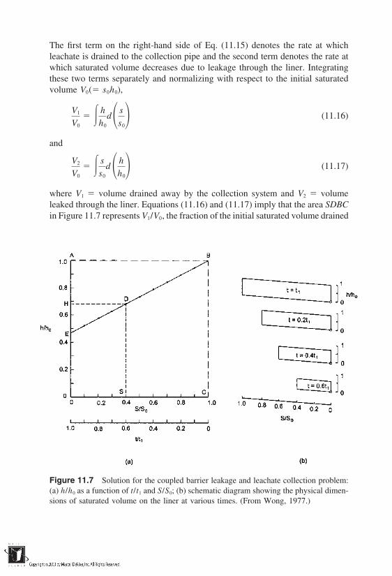
The first term on the right-hand side of Eq. (11.15) denotes the rate at whichleachate is drained to the collection pipe and the second term denotes the rate atwhich saturated volume decreases due to leakage through the liner. Integratingthese two terms separately and normalizing with respect to the initial saturatedvolume V0( s0h0),

V1

V0

h

h0

d s

s0 (11.16)

and

V2

V0

s

s0

d h

h0 (11.17)

where V1 volume drained away by the collection system and V2 volumeleaked through the liner. Equations (11.16) and (11.17) imply that the area SDBCin Figure 11.7 represents V1/V0, the fraction of the initial saturated volume drained

Figure 11.7 Solution for the coupled barrier leakage and leachate collection problem:(a) h/h0 as a function of t/t1 and S/S0; (b) schematic diagram showing the physical dimen-sions of saturated volume on the liner at various times. (From Wong, 1977.)

away by the leachate collection system, while the area ABDH represents V2/V0,the fraction of the initial saturated volume that has leaked through the liner. Thus,Figure 11.7 serves as a graphical solution for the apportionment of initial satu-rated volume at time t 0.6t1 (point S). The area OHDS represents the fractionof the initial saturated volume that still remains on the liner. V1/V0 is often referredas the collection efficiency of the drains. Thus, the closer the point E is to pointA, the greater is the collection efficiency. In reality, E will never coincide withA because of the leakage through the liner. From a design standpoint, however,the parameters involved in Eq. (11.12) must be chosen such that E is as closeto A as possible. Despite the numerous assumptions made in Wong’s model, itis one of the useful models available at present to apportion leachate. A detailedevaluation of the model and the effects of various design parameters on the appor-tionment are provided by Wong (1977) and Kmet et al. (1981).

11.5 FLOW AND TRANSPORT THROUGH BARRIERS

As stated earlier, the apportionment of leachate between the barrier leakage andthe collection system is a single problem. However, it is customary to separ-ate the leachate collection system design from the barrier design. While designingthe barrier, the head of leachate mound is assumed to be constant, to simplifythe flow problem. For a conservative estimate of leakage through the barrier, theleachate mound may be assumed to be at its maximum elevation, since the leak-age estimate will be higher under this assumption.

When considering the leakage through the barrier, it is important to keepin mind that both quality and quantity of leakage govern the impact of the wastecontainment system on the surrounding soil and groundwater resources. Thus, asignificant leakage of ‘‘relatively clean’’ water might be more acceptable than aninsignificant leakage of highly contaminated water. Earlier regulations of wastecontainment systems were based on fixing the quantity of leakage through thebarrier, viz., the leakage rate should not exceed 1.65 in./year, the hydraulic con-ductivity of the barrier should not exceed 1 107 cm/s, etc. As such, thesequantity-based criteria value the advective transport of contaminants through thebarrier with little regard to the effects of dispersion mechanism. More recentcriteria for the performance of waste containment systems consider all the masstransport mechanisms. The performance criteria for waste containment systemsmay thus be studied under two broad categories:

1. Quantity-based criteria, which limit the overall leakage rate throughthe barrier, perhaps by fixing the hydraulic conductivity and the thick-ness of the barrier

2. Quality-based criteria, which limit the exit leachate concentrations orfluxes during the design life-period of the system

We will consider these two by considering the flow and transport phenomenathrough barriers separately.

11.5.1 Flow Through Barriers

For a simple configuration of a soil barrier underlain by subsoil (Fig. 11.8), Dar-cy’s law can be used to estimate the flow rate. The pore velocity through thebarrier, Va, will be maximum under fully saturated conditions; therefore,

Va ksi

n(11.18)

where ks saturated hydraulic conductivity of the barrier [L/T], i hydraulicgradient (dimensionless), and n porosity of the barrier (dimensionless). Thetransit time through the barrier, t, may therefore be expressed as

t d

Va

dn

ksi(11.19)

Figure 11.8 Schematic of a soil barrier layer underlain by a subsoil.

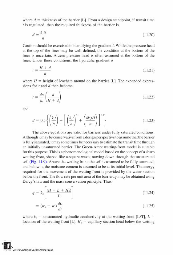
where d thickness of the barrier [L]. From a design standpoint, if transit timet is regulated, then the required thickness of the barrier is

d ksit

n(11.20)

Caution should be exercised in identifying the gradient i. While the pressure headat the top of the liner may be well defined, the condition at the bottom of theliner is uncertain. A zero-pressure head is often assumed at the bottom of theliner. Under these conditions, the hydraulic gradient is

i H d

d(11.21)

where H height of leachate mound on the barrier [L]. The expanded expres-sions for t and d then become

t dn

ks d

H d (11.22)

and

d 0.5 kst

n kst

n 2

4kstH

n 0.5

(11.23)

The above equations are valid for barriers under fully saturated conditions.Although it may be conservative from a design perspective to assume that the barrieris fully saturated, it may sometimes be necessary to estimate the transit time throughan initially unsaturated barrier. The Green-Ampt wetting-front model is suitablefor this purpose. This is a phenomenological model based on the concept of a sharpwetting front, shaped like a square wave, moving down through the unsaturatedsoil (Fig. 11.9). Above the wetting front, the soil is assumed to be fully saturated;and below it, the moisture content is assumed to be at its initial level. The energyrequired for the movement of the wetting front is provided by the water suctionbelow the front. The flow rate per unit area of the barrier, q, may be obtained usingDarcy’s law and the mass conservation principle. Thus,

q ku (H L Hd)L (11.24)

(ws wi)dL

dt(11.25)

where ku unsaturated hydraulic conductivity at the wetting front [L/T], L location of the wetting front [L], Hd capillary suction head below the wetting

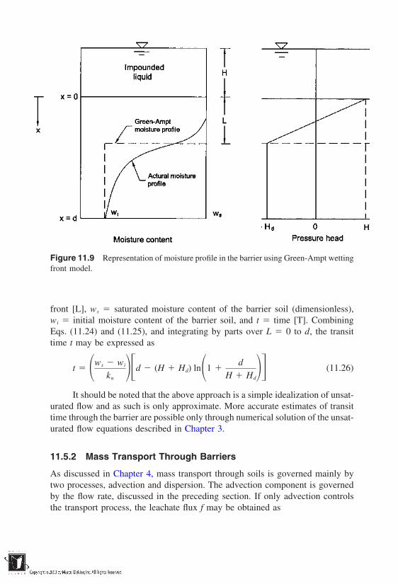
Figure 11.9 Representation of moisture profile in the barrier using Green-Ampt wettingfront model.

front [L], ws saturated moisture content of the barrier soil (dimensionless),wi initial moisture content of the barrier soil, and t time [T]. CombiningEqs. (11.24) and (11.25), and integrating by parts over L 0 to d, the transittime t may be expressed as

t ws wi

kud (H Hd) ln1

d

H Hd (11.26)

It should be noted that the above approach is a simple idealization of unsat-urated flow and as such is only approximate. More accurate estimates of transittime through the barrier are possible only through numerical solution of the unsat-urated flow equations described in Chapter 3.

11.5.2 Mass Transport Through Barriers

As discussed in Chapter 4, mass transport through soils is governed mainly bytwo processes, advection and dispersion. The advection component is governedby the flow rate, discussed in the preceding section. If only advection controlsthe transport process, the leachate flux f may be obtained as

f VC0 (11.27)

where f leachate flux [M/L2T], V seepage velocity [L/T], and C0 sourceconcentration [M/L3] at the top of the barrier, assumed to be constant. Takingthe other extreme position that dispersion is the only process governing the lea-chate flux, f may be obtained using Fick’s first law as

f nD∂C

∂L nD

C0

d(11.28)

where D dispersion coefficient [L2/T], which accounts for both molecular dif-fusion and hydrodynamic dispersion, and ∂C/∂L is the concentration gradient,which is assumed to be steady under a constant concentration of C0 at the topand zero concentration at the bottom of the barrier. It should be noted that theconcentrations at the boundaries may be such that steady-state concentration gra-dients may never exist. For instance, in the cases where the bottom of the barrieris not flushed with clean water, the outlet concentrations will keep on increasinguntil they approach the inlet concentration C0. Beyond this stage, the concentra-tion gradients (and consequently the diffusion process) cease to exist in the liner.Also, it may not be appropriate to assume that the inlet concentrations C0 areconstant, since the contaminant mass is finite and the source is exhausted as theleachate travels out of the barrier. Even if the boundary conditions at the inletand outlet of the barrier are favorable for steady concentration gradients, a sig-nificant time period elapses before such steady-state conditions occur.

To account for time-dependent transport of contaminants through the bar-rier, Fick’s second law may be used. According to this law,

∂C

∂ t D

∂ 2C

∂x2(11.29)

where D dispersion coefficient, which accounts for both molecular diffusionand hydrodynamic dispersion. The solution for Eq. (11.29), discussed in Chapter4, is expressed as

C

C0

erfc x

2√Dt (11.30)

This solution is shown schematically in Figure 11.10. Under pure dispersion con-ditions, Eq. (11.30) may be used to obtain the time it takes for the concentrationsat the outlet of the barrier to reach a specified value.

When both advection and dispersion are to be considered in the mass trans-port modeling, the appropriate solutions discussed in Chapter 4 for the advection-dispersion equation may be used. The solution commonly employed is that ofOgata and Banks (1961), which gives concentrations C as a function of time t

Figure 11.10 Schematic profiles of leachate concentrations at various times in the soilbarrier.

and depth x beneath the surface of a barrier, when it is assumed to be infinitelydeep and subject to the following initial and boundary conditions:

C(x, 0) 0 x 0 (11.31a)C(0, t) C0 t 0 (11.31b)C(∞, t) 0 t 0 (11.31c)

In the absence of decay, the solution to the advection-dispersion equation is thesame as Eq. (4.70), which is rewritten here.

C(x, t) C0

2 erfcRx Vxt

2√RDxt expVxx

DxRx Vxt

2√RDxt (4.70)

This solution is often expressed in terms of dimensionless variables as follows:

C(x, t) C0

2 erfc1 T

2√T/P exp(P)1 T

2√T/P (11.32)

where

T Vxt

Rx

Vxt

Rd at x d

(11.33)

and

P Vxx

Dx

Vxd

Dx

at x d

(11.34)

T indicates effective pore volumes of flow, and P is the Peclet number definedwith respect to the barrier thickness d.

Once the concentrations C(x, t) are known at the outlet of the barrier, thetotal flux f may be obtained by summing the advection and dispersion compo-nents. Shackelford (1990) expressed the total flux in a dimensionless form usinga dimensionless flux number, FN, as follows:

FN fd

nC0Dx

12

(PQ1 Q2) (11.35)

where

Q1 erfc1 T

2√T/P (11.36a)

and

Q2

2 exp(1 T)/2√T/P2

√πT/P

(11.36b)

To aid in the design process, Eqs. (11.32) and (11.35) are reduced to agraphical form (Shackelford, 1990). Using these graphs, C(x, t) and FN may beobtained for specified values of T and P. Shackelford (1990) suggests an iterativeprocedure using these solutions to obtain a design thickness of the barrier. Theprocedure involves the following steps:

1. Assume a liner thickness, d.2. Calculate P using Eq. (11.34).3. Determine T for a specified value of either C/C0 or f using Eq. (11.32)

or (11.35).4. Use Eq. (11.33) to determine the transit time t.5. Repeat steps 1–4 until t is greater than or equal to the design life of

the containment system.

The above solutions are valid for simplified initial and boundary conditions de-scribed in Eq. (11.31). The boundary condition C C0 at the inlet is not anaccurate one, since it represents discontinuity at the liquid–soil interface andviolates the mass conservation principle. Solutions for more realistic boundaryconditions are given by Van Genuchten and Alves (1982). However, the solutionsgiven above are fairly accurate with differences up to only 5% when comparedwith the more accurate solutions (Gershon and Nir, 1969).

Booker and Rowe (1987) considered the effect of finite nature of contami-nant source on the mass transport through barrier. In contrast to the boundarycondition represented in Eq. (11.31b), they assumed that the finite mass of con-taminant within the landfill could be represented in terms of an equivalent heightof leachate, Hf. The analytical solution obtained by Booker and Rowe (1987) forcontaminant transport in an infinitely deep deposit as the source concentrationvaried with time is as follows:

C(x, t) C0 exp(ab b2t)

(b c)[bf (b, t) cf (c, t)] (11.37)

where

f (b, t) exp(ab b2t) erfc a

2√t b√t (11.38)

f (c, t) exp(ac c2t) erfc a

2√t c√t (11.39)

a xn ρbKd

nDx

1/2

(11.40)

b Vx n

4Dx(n ρbKd)1/2

(11.41)

c nDx

Hfn ρbKd

nDx

1/2

b (11.42)

where ρb and Kd are dry mass density and distribution coefficient, respectively.The function f (p, t) (for p b or p c) may be simplified as

f(p, t) expa2

4t φ(α) (11.43)

Figure 11.11 φ(α) as a function of α in Booker and Rowe’s solution.

where α (p √t a/2√t) and the function φ(α) is given in Fig. 11.11. Notethat with some algebraic manipulation, it could be shown that Eq. (11.37) reducesto Eq. (4.70) for Hf → α (i.e., c b).

11.5.3 Relative Importance of Advection and Dispersion

Considering the impermeable nature of barrier materials, it is tempting to ignoreadvection process and assume that only dispersion governs the leachate transport.However, several studies illustrated that neglecting advection may lead to errone-ous and unconservative estimates of leachate flux for typical landfill scenarios(Rowe, 1987; Shackelford, 1988). Figure 11.12, for instance, shows the concen-tration profiles in and chemical flux through a 1.2-m clay liner with and withoutadvective component of mass transport. The seepage velocity (0.006 m/year)considered in this study is representative of clay liners with hydraulic conductivi-ties less than 1 107 cm/s and subjected to hydraulic gradients less than 0.2.It is seen in the figure that not only are the concentrations in the liner greaterwhen advection is considered, the concentration gradients (which govern the lea-chate fluxes) at the bottom of the liner are also greater. In general, as the seepagevelocity is increased with all other factors kept constant, the concentrations inthe liner as well as the fluxes exiting the liner are increased. For the same condi-tions, Figure 11.12b illustrates the time-dependent fluxes exiting the liner under

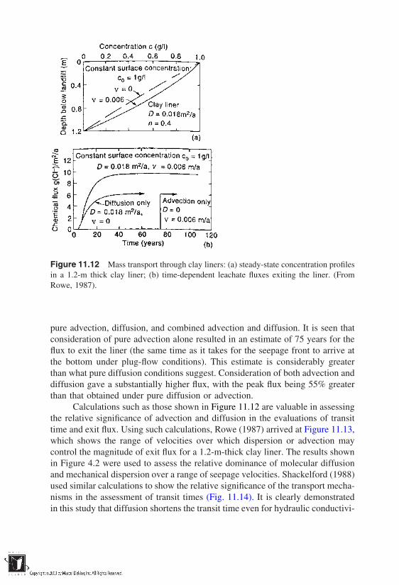
Figure 11.12 Mass transport through clay liners: (a) steady-state concentration profilesin a 1.2-m thick clay liner; (b) time-dependent leachate fluxes exiting the liner. (FromRowe, 1987).

pure advection, diffusion, and combined advection and diffusion. It is seen thatconsideration of pure advection alone resulted in an estimate of 75 years for theflux to exit the liner (the same time as it takes for the seepage front to arrive atthe bottom under plug-flow conditions). This estimate is considerably greaterthan what pure diffusion conditions suggest. Consideration of both advection anddiffusion gave a substantially higher flux, with the peak flux being 55% greaterthan that obtained under pure diffusion or advection.

Calculations such as those shown in Figure 11.12 are valuable in assessingthe relative significance of advection and diffusion in the evaluations of transittime and exit flux. Using such calculations, Rowe (1987) arrived at Figure 11.13,which shows the range of velocities over which dispersion or advection maycontrol the magnitude of exit flux for a 1.2-m-thick clay liner. The results shownin Figure 4.2 were used to assess the relative dominance of molecular diffusionand mechanical dispersion over a range of seepage velocities. Shackelford (1988)used similar calculations to show the relative significance of the transport mecha-nisms in the assessment of transit times (Fig. 11.14). It is clearly demonstratedin this study that diffusion shortens the transit time even for hydraulic conductivi-

Figure 11.13 Range of Darcy velocities over which diffusion, mechanical dispersion,and advection control the magnitude of the exit flux (Rowe, 1987).

ties of the order of 107 cm/s. It becomes a dominant transport process at hydrau-lic conductivities less than 2 108 cm/s.

It should be noted that the directions in which mass transport occurs dueto advection and dispersion may not always be the same. Figure 11.15 showsthree transport scenarios, which warrant consideration when assessing the transit

Figure 11.14 Transit times corresponding to C/C0 0.5 as a function of hydraulicconductivity for a hypothetical 3-ft clay liner with an average porosity of 0.50 and sub-jected to a hydraulic gradient of 1.33. A diffusion coefficient of 6 106 cm2/s wasassumed. (From Shackelford, 1988.)

Figure 11.15 Transport scenarios involving different directions of advection and diffu-sion.

times and exit fluxes. Figure 11.15a shows the situation where both advectionand diffusion follow the same direction and the above discussion is valid. Figure11.15b illustrates a more favorable scenario, where the hydrogeology at the con-tainment system is such that flow is directed into the waste. An example is theplacement of the containment system below the groundwater table and controllingthe flow into the waste using an internal leachate collection system. The advectionprocess in this case opposes the outward diffusion flux of contaminants. Gradientreversal may also be achieved using a continuous or periodic application of elec-

tric gradients across the barrier (Fig. 11.15c). An electroosmotic counterflow isgenerated to oppose the flow due to advection and dispersion. Gradient reversalsare often viewed as attractive methods in dealing with cracks and macropores inthe barriers, which may participate in the counterflow and prevent outward leak-age. Evaluation of transit time and exit flux magnitudes in these cases requiresa good handle on the mechanisms that cause gradient reversals.

11.6 STABILITY OF WASTE CONTAINMENT SYSTEMS

In addition to minimizing the flow of leachate into the surrounding soil andgroundwater, a waste containment system should retain its structural integrityduring its design life. The structural stability of the containment system as awhole or of its individual components controls its key function of containing thewaste. For instance, excessive settlements of the landfill material might disruptthe top cover of the system. The settlements of foundation soils might damagethe leachate collection system and bottom liner, and allow leachate to exit thesystem freely. Similarly, slope failures of the structure, either local or systemic,would lead to catastrophic consequences.

It should be noted that the conditions that are favorable for low hydraulicconductivity may not necessarily be favorable from a stability point of view. Forinstance, the compaction parameters leading to low hydraulic conductivity ofcompacted clays may not be favorable for high interface strengths between theclays and geomembranes (Seed and Boulanger, 1991; Stark and Poeppel, 1994).Thus, in the design phase of a waste containment system, both flow and stabilityshould be given equal importance, and construction parameters acceptable fromboth viewpoints must be chosen.

Stability analyses for waste containment systems are complicated primarilybecause of the following reasons.

1. The properties of the waste are both spatially and temporally variable.It is difficult to obtain representative samples and conduct routinegeotechnical tests to determine their properties. Some studies even sug-gest that a Mohr-Coulomb representation of shear strength, commonlyused in geotechnical engineering, may not be appropriate for wastematerials (Mitchell et al., 1995).

2. A given containment system may contain components made up of anumber of different materials, which are diverse in their stress–strainproperties as shown in Figure 11.16. The differences in these propertiescreate compatibility problems at the interfaces between various compo-nents. The deformations required to mobilize the peak strengths of theindividual materials could be significantly different.

Figure 11.16 Diverse stress–strain properties of material components in a containmentsystem (Mitchell et al., 1995).

3. The modes of failure are not well established. For instance, slope fail-ure for a containment system may not follow the rotational mode com-monly used in geotechnical engineering.

Because of these complexities, stability analyses for waste containmentstructures have not been well established. Initial efforts involve extrapolation ofexisting analyses available for pure soils in geotechnical engineering. Three is-sues of stability are of broad importance in the case of waste containment sys-tems:

1. Local and systemic failures of slopes2. Stability of the interfaces between various components, primarily be-

tween geotextile/geomembrane and soil3. Total and differential settlements of the system

A detailed discussion of these issues is provided in the following subsections.

11.6.1 Slope Stability

Slope failures in containment systems fall under three broad categories, as shownin Figure 11.17. The failures may occur either within the waste material or across

Figure 11.17 Potential slope failure modes in landfills (Mitchell et al., 1995).

the foundation soil and soil–liner interfaces. The mode of failure is uncertain inthese types of failures, but generally, a rotational type of failure shown in thefigure is considered to be the most probable mode. With this idealization, thestability analysis will reduce to the common geotechnical problem of assessingthe stability of a natural slope or a man-made embankment.

Traditional methods of slope stability analysis evaluate shear stresses caus-ing failure along an assumed surface and compare them with the shear strengthmobilized. The ratio of shear strength to shear stress is taken as the factor of safetyagainst failure. In the method of slices, commonly used to assess the stability offinite slopes, the mass of soil is divided into a number of segments and the forceson each segment are evaluated (Fig. 11.18). Considering the slice abcd, for in-stance, the forces consist of the weight of the slice, the normal and shear forcesacting on the failure surface cd, and the normal and shear forces acting on thevertical faces ad and bc. An approximate solution is possible when certain as-sumptions are made concerning the forces on the vertical faces. Assuming thatthe resultants of Pi and Ti are equal to Pil and Til, the normal and shear forceson surface cd may be obtained as

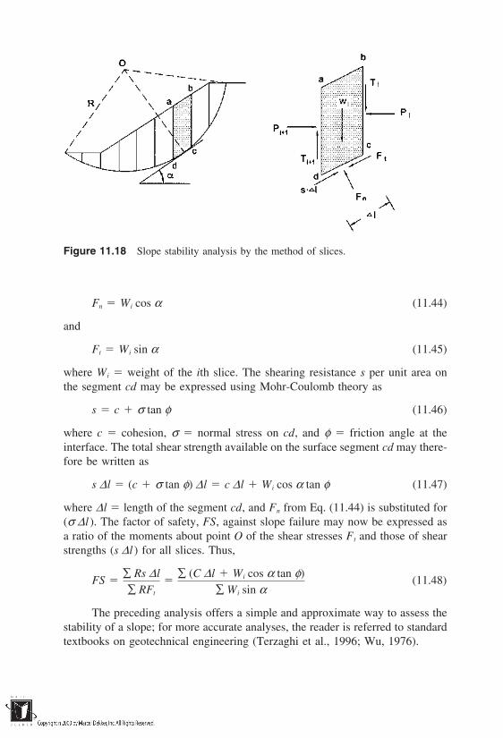
Figure 11.18 Slope stability analysis by the method of slices.

Fn Wi cos α (11.44)

and

Ft Wi sin α (11.45)

where Wi weight of the ith slice. The shearing resistance s per unit area onthe segment cd may be expressed using Mohr-Coulomb theory as

s c σ tan φ (11.46)

where c cohesion, σ normal stress on cd, and φ friction angle at theinterface. The total shear strength available on the surface segment cd may there-fore be written as

s ∆l (c σ tan φ) ∆l c ∆l Wi cos α tan φ (11.47)

where ∆l length of the segment cd, and Fn from Eq. (11.44) is substituted for(σ ∆l ). The factor of safety, FS, against slope failure may now be expressed asa ratio of the moments about point O of the shear stresses Ft and those of shearstrengths (s ∆l ) for all slices. Thus,

FS ∑ Rs ∆l

∑ RFt

∑ (C ∆l Wi cos α tan φ)

∑ Wi sin α(11.48)

The preceding analysis offers a simple and approximate way to assess thestability of a slope; for more accurate analyses, the reader is referred to standardtextbooks on geotechnical engineering (Terzaghi et al., 1996; Wu, 1976).

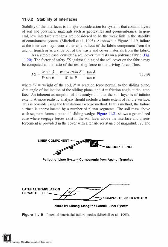
11.6.2 Stability of Interfaces

Stability of the interfaces is a major consideration for systems that contain layersof soil and polymeric materials such as geotextiles and geomembranes. In gen-eral, low interface strengths are considered to be the weak link in the stabilityof containment systems (Mitchell et al., 1995). As shown in Figure 11.19, failureat the interface may occur either as a pullout of the fabric component from theanchor trench or as a slide-out of the waste and cover materials from the fabric.

As a simple case, consider a soil cover that rests on a polymer fabric (Fig.11.20). The factor of safety FS against sliding of the soil cover on the fabric maybe computed as the ratio of the resisting force to the driving force. Thus,

FS N tan δW sin θ

W cos θ tan δ

W sin θ

tan δtan θ

(11.49)

where W weight of the soil, N reaction force normal to the sliding plane,θ angle of inclination of the sliding plane, and δ friction angle at the inter-face. An inherent assumption of this analysis is that the soil layer is of infiniteextent. A more realistic analysis should include a finite extent of failure surface.This is possible using the translational wedge method. In this method, the failuresurface is approximated by a number of planar segments. The soil mass aboveeach segment forms a potential sliding wedge. Figure 11.21 shows a generalizedcase where seepage forces exist in the soil layer above the interface and a rein-forcement is provided in the cover with a tensile resistance of magnitude, T. The

Figure 11.19 Potential interfacial failure modes (Mitchell et al., 1995).

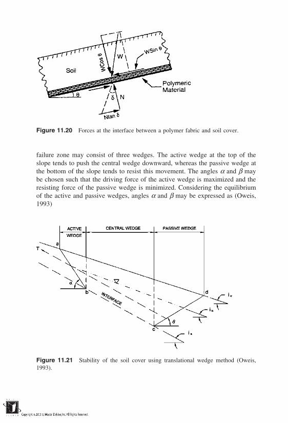
Figure 11.20 Forces at the interface between a polymer fabric and soil cover.

failure zone may consist of three wedges. The active wedge at the top of theslope tends to push the central wedge downward, whereas the passive wedge atthe bottom of the slope tends to resist this movement. The angles α and β maybe chosen such that the driving force of the active wedge is maximized and theresisting force of the passive wedge is minimized. Considering the equilibriumof the active and passive wedges, angles α and β may be expressed as (Oweis,1993)

Figure 11.21 Stability of the soil cover using translational wedge method (Oweis,1993).

tan α tan φ √1 tan2 φ tan ic/sin φ cos φ (11.50)

and

tan β tan φ √1 tan2 φ tan ic/sin φ cos φ (11.51)

Note that for a horizontal surface (ic 0), the angles reduce to α 45 φ/2,and β 45 φ/2, which must be familiar to students of geotechnical engi-neering. The factor of safety against sliding at the interface may be obtained byconsidering the force balance of the central wedge. The forces acting on thecentral wedge are essentially the active and passive forces on the sides of thewedge, the weight of the wedge, and the resistance available at the failure surfacebc. For the simplest, and also the most practical, case of a soil cover of uniformthickness with a groundwater level parallel to the interface, the stability equationfor the central wedge will yield the factor of safety as (Oweis, 1993)

FS 1

(1 t) c

γh sin is cos is

tan δ i

tan is1

γ whw

γh (11.52)

where

t T

Wc sin is

(11.53)

Wc weight of the central wedgec cohesion of the soilγ unit weight of the soilh thickness of the coverδ i angle of friction at the interfaceγw unit weight of waterhw uniform thickness of the saturated layer of the cover.

Stability analyses for the soil cover are also available for other simplifiedconditions of the failure surface. For instance, Giroud and Beech (1989) and theU.S. EPA (1991) document analyses for the condition of a horizontal failuresurface in the passive wedge of the soil. These analyses are useful from a designstandpoint to determine the thickness of the soil cover, and whether and howmuch tensile reinforcement is required to achieve a desired factor of safety againstslope failure.

Another important consideration regarding the interfacial stability is thecompatibility of frictional stresses developed at the top and bottom faces of ageomembrane. Typically, geomembranes are located at the interface of two dif-ferent materials, and the differences in frictional stresses may cause excessiveshearing stresses in the geomembrane. The tensile strength of the geomembrane

should be such that it can withstand these differences with an adequate factor ofsafety.

11.6.3 Settlements

There are significant differences between soil and waste materials in terms ofthe settlement mechanisms. Settlement analyses for waste materials are com-plicated because of the inherent heterogeneity, their decomposition, and short-term and long-term environmental conditions affecting the composition ofthe materials. The mechanisms involved in waste settlements are several (Edilet al., 1990; Sowers, 1973): (1) particle reorientation; (2) raveling, or movementof fine particles into large voids; (3) physicochemical changes including corro-sion, combustion, and oxidation of the waste materials; (4) biochemical decom-position; (5) dissolution of soluble materials; and (6) plastic flow and creep.Edil et al. (1990) noted that refuse fills typically settle from 5% to 30% of theiroriginal thickness under self-weight, and the magnitude of the settlement dependson factors such as degree of initial compaction, waste composition, and envi-ronmental conditions. The primary settlement is generally known to occur rela-tively rapidly, between 1 month and 5 years after the waste placement. Unlikethe case of pure soils, the secondary settlements are known to be relatively sig-nificant.

Although initial efforts (Sowers, 1973; Oweis and Khera, 1990) relied onone-dimensional consolidation theory to approximate settlements of waste fills[Eqs. (1.16)–(1.18)], application of the theory to waste materials is generallyestablished to be of limited validity. This is because the e versus log σ curvemay exhibit nonlinearity, and several of the parameters required, such as com-pression and rebound indices, change with time and cannot be determined ade-quately (Fassett, et al., 1993). Edil et al. (1990) evaluated two models, the Gibson-Lo model and the power creep law, using compressibility data from five sites.The former is a rheological representation of the soil using a spring to representprimary compression and a parallel dashpot to represent secondary compression.The time-dependent settlement based on the Gibson and Lo model may be ex-pressed as

S(t) H ∆σa b1 expλbt (11.54)

where

S(t) settlement at time tH initial height of waste material

∆σ change in overburden pressure

a primary compressibility parameterb secondary compressibility parameter

λb

rate of secondary compression

The power creep law is useful to represent the creep behavior of materialsand is generally expressed as

S(t) H ∆σ m t

tr

n

(11.55)

where

m reference compressibilityn compression ratetr reference timet time since load application

Based on the limited data, Edil et al. (1990) reported that the Gibson andLo model estimated settlements within 2% and 20% of actual settlements, andthe power creep law estimated settlements within 0–14%.

An important effect of the waste settlement is to deform the cover systemand strain the polymeric barriers. Estimation of these deformations is difficultand necessarily involves assumptions related to settlement trough geometry andwaste-volume reduction rate. The soil arching theory and the tensioned membranetheory may be used to estimate stresses that develop in geomembranes placedwithin soil covers overlying void spaces (Giroud et al., 1988; Knipshield, 1985).Knipshield (1985) developed a semiempirical procedure for estimating the designratio (analogous to the factor of safety) for geomembranes that settle. The designratio (DR) is estimated as

DR γr

γu

(11.56)

where

γr geomembrane rupture strain (%)γu uniform strain on the geomembrane (%)

The rupture strain, γr, of the geomembrane is determined from a load versusstrain curve as shown in Figure 11.22. The uniform strain, γu, may be obtainedfrom Figure 11.23. The settlement, S, may be estimated as a fraction of the thick-ness of the waste, and the width of the waste storage cell may be used as thewidth of the settled area (2L in Fig. 11.23). As seen in the figure, the uniform

Figure 11.22 A typical load–strain curve for geomembranes.

Figure 11.23 A graphical method to estimate uniform strain under triangular and circu-lar trough assumptions (Knipshield, 1985).

strain estimate is dependent on the approximation of the trough geometry, trian-gular or circular.

11.6.4 Geotechnical Properties of Waste

The accuracy of the stability analyses outlined above is limited by the uncertaintyand variability involved in the properties of waste. Several attempts have beenreported in the literature to determine the engineering properties of waste. Theproperties of materials required in stability analyses of waste containment sys-tems may be discussed under four categories:

1. Unit weight of waste2. Shear strength of waste3. Shear strength properties at the interfaces between various components4. Compressibility of the waste

The unit weight of waste materials varies within a broad range, becauseof several factors: (1) type and origin of the waste; (2) mode of operation of thecontainment system and placement techniques; (3) degree of compaction used;(4) age of the waste after placement, which governs the environmental effectssuch as biochemical decomposition; and (5) depth at which waste is located inthe system. In general, the unit weight of the waste is believed to increase withdepth in the containment system (Fassett et al., 1993). The ranges of unit weightvalues reported in the literature are summarized in Table 11.10. It is importantto note that these values were obtained based on a limited number of site andwaste-specific observations, and as such, are useful only in preliminary evalua-tions.

As mentioned earlier, it is difficult to assess the shear strength of wastematerials because of the questionable validity of the Mohr-Coulomb theory itself.However, due to lack of stress–strain characterizations of the materials, the indus-try continues to adopt this theory as an approximate guide in the design of con-tainment systems. A number of studies have been reported in the literature thatinvolve determination of cohesion and friction angle of waste materials. The pa-rameters were estimated using one of three approaches: (1) direct laboratory test-ing on waste materials using direct shear and triaxial tests (Fang et al., 1977; EarthTechnology Corporation, 1988); (2) back-calculation from field tests (Converse,Davis, Dixon Associates, 1975); and (3) in-situ testing of the materials using vaneshear test and by correlating SPT values to strength properties (Earth TechnologyCorporation, 1988). Based on a summary of the various studies, Singh and Mur-phy (1990) documented the range of recommended strengths of municipal solidwaste in terms of a relationship between cohesion and friction angle (Fig. 11.24).Due to the large scatter in the data, it is advisable to use the lower bound of theshaded area in preliminary investigations. Similar to the municipal waste, mineral

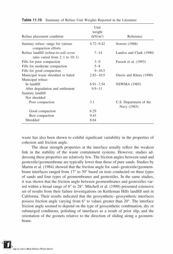
Table 11.10 Summary of Refuse Unit Weights Reported in the Literature

Unitweight

Refuse placement condition (kN/m3) Reference

Sanitary refuse: range for various 4.72–9.42 Sowers (1968)compaction efforts

Refuse landfill (refuse-to-soil cover 7–14 Landva and Clark (1990)ratio varied from 2:1 to 10:1)

Fills for poor compaction 3–9 Fassett et al. (1993)Fills for moderate compaction 5–8Fills for good compaction 9–10.5Municipal waste shredded or baled 2.83–10.5 Oweis and Khera (1990)Municipal refuse:

In landfill 6.91–7.54 NSWMA (1985)After degradation and settlement 9.9–11

Sanitary landfillNot shredded

Poor compaction 3.1 U.S. Department of theNavy (1983)

Good compaction 6.29Best compaction 9.43

Shredded 8.64

waste has also been shown to exhibit significant variability in the properties ofcohesion and friction angle.

The shear strength properties at the interface usually reflect the weakestlink in the stability of the waste containment systems. However, studies ad-dressing these properties are relatively few. The friction angles between sand andgeotextile/geomembrane are typically lower than those of pure sands. Studies byMartin et al. (1984) showed that the friction angle for sand–geotextile/geomem-brane interfaces ranged from 17° to 30° based on tests conducted on three typesof sands and four types of geomembranes and geotextiles. In the same studies,it was shown that the friction angle between geomembranes and geotextiles var-ied within a broad range of 6° to 28°. Mitchell et al. (1990) presented extensiveset of results from their failure investigations on Kettleman Hills landfill unit inCalifornia. Their results indicated that the geosynthetic–geosynthetic interfacespossess friction angle varying from 6° to values greater than 20°. The interfacefriction angle seemed to depend on the type of geosynthetic combination, dry orsubmerged conditions, polishing of interfaces as a result of prior slip, and theorientation of the geonets relative to the direction of sliding along a geomem-brane.

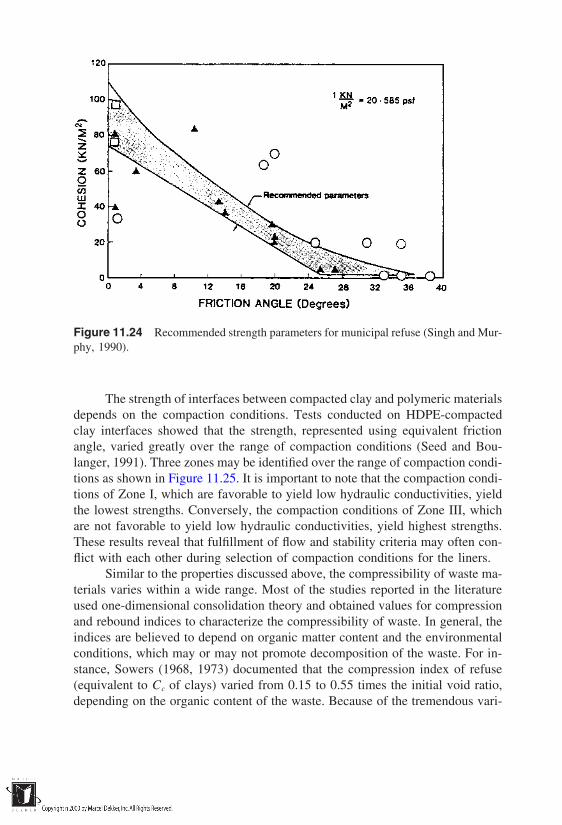
Figure 11.24 Recommended strength parameters for municipal refuse (Singh and Mur-phy, 1990).

The strength of interfaces between compacted clay and polymeric materialsdepends on the compaction conditions. Tests conducted on HDPE-compactedclay interfaces showed that the strength, represented using equivalent frictionangle, varied greatly over the range of compaction conditions (Seed and Bou-langer, 1991). Three zones may be identified over the range of compaction condi-tions as shown in Figure 11.25. It is important to note that the compaction condi-tions of Zone I, which are favorable to yield low hydraulic conductivities, yieldthe lowest strengths. Conversely, the compaction conditions of Zone III, whichare not favorable to yield low hydraulic conductivities, yield highest strengths.These results reveal that fulfillment of flow and stability criteria may often con-flict with each other during selection of compaction conditions for the liners.

Similar to the properties discussed above, the compressibility of waste ma-terials varies within a wide range. Most of the studies reported in the literatureused one-dimensional consolidation theory and obtained values for compressionand rebound indices to characterize the compressibility of waste. In general, theindices are believed to depend on organic matter content and the environmentalconditions, which may or may not promote decomposition of the waste. For in-stance, Sowers (1968, 1973) documented that the compression index of refuse(equivalent to Cc of clays) varied from 0.15 to 0.55 times the initial void ratio,depending on the organic content of the waste. Because of the tremendous vari-

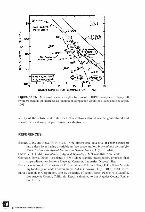
Figure 11.25 Measured shear strengths for smooth HDPE—compacted clayey till(with 5% bentonite) interfaces as function of compaction conditions (Seed and Boulanger,1991).

ability of the refuse materials, such observations should not be generalized andshould be used only in preliminary evaluations.

REFERENCES

Booker, J. R., and Rowe, R. K. (1987). One dimensional advective-dispersive transportinto a deep layer having a variable surface concentration. International Journal forNumerical and Analytical Methods in Geomechanics, 11(2):131–142.

Chow, V. T. (1964). Handbook of Applied Hydrology. McGraw-Hill, New York.Converse, Davis, Dixon Associates. (1975). Slope stability investigation, proposed final

slope adjacent to Pomona Freeway. Operating Industries Disposal Site.Demetracopoulos, A. C.,Korfiatis, G. P., Bourodimos, E.L., and Nawy, E. G. (1984). Model-

ing for design of landfill bottom liners. ASCE J. Environ. Eng., 110(6): 1084–1098.Earth Technology Corporation. (1988). Instability of landfill slope, Puente Hills Landfill,

Los Angeles County, California. Report submitted to Los Angeles County Sanita-tion District.

Edil, T. B., Ranguette, V. J., and Wuellner, W. W. (1990). Settlement of municipal re-fuse. In Geotechnics of Waste Fills: Theory and Practice, ASTM STP 1070, A.Landva and G. D. Knowles, eds., American Society for Testing and Materials, Phil-adelphia.

Ehrig, H. J., and Scheelhaase, T. (1993). Pollution potential and long term behaviour ofsanitary landfills. Proc. Fourth Int. Landfill Symp., Cagliari, Italy, pp. 1204–1225.

Fang, H. Y., et al. (1977). Strength testing of bales of sanitary landfill. Fritz EngineeringLaboratory, Department of Civil Engineering, Lehigh University.

Fassett, J. B., Leonards, G. A., and Repetto, P. C. (1993). Geotechnical properties ofmunicipal solid wastes and their uses in landfill design. Proc. Waste Tech 93 Conf.

Fenn, D. G., Hanley, K. J., and DeGeare, T. V. (1975). Use of the water balance methodfor predicting leachate generation from solid waste disposal sites, EPA/530/SW-168. U.S. Environmental Protection Agency, Cincinnati, OH.

Gershon, N. D., and Nir, A. (1969). Effects of boundary conditions of models on tracer distri-bution in flow through porous mediums. Water Resources Research, 5(4):830–839.

Giroud, J. P., and Beech, J. F. (1989). Stability of soil layers on geosynthetic lining sys-tems. Geosynthetics ’89, IFAI, San Diego, CA.

Giroud, J. P., Bonaparte, R., Beech, J. F., and Gross, B. A. (1988). Load-carrying capacityof a soil layer supported by a geosynthetic overlying a void. Proc. Int. Symp. onTheory and Practice of Earth Reinforcement, Fukuoka, Japan, pp. 185–190.

Horton, R. E. (1919). Rainfall interception. Monthly Weather Review, U.S. Weather Bu-reau, 47(9):603–623.

Kmet, P. (1982). EPA’s water balance method—Its uses and limitations. Wisconsin Depart-ment of National Resources, Bureau of Solid Waste Management, Madison, WI.

Kmet, P., et al. (1981). Analysis of design parameters affecting the collection efficiencyof clay lined landfills. Proc. 4th Annual Madison Conf. of Applied Research andPractice on Municipal and Industrial Waste.

Knipshield, F. W. (1985). Material selection and dimensioning of geomembranes forgroundwater protection. Waste and Refuse, 22.

Knisel, W. G., ed. (1980). CREAMS, a field-scale model for chemical runoff and erosionfrom agricultural management systems, Vols. I, II, and III. USDA-SEA-AR Conser-vation Research Report 26.

Korfiatis, G. P., and Demetracopoulos, A. C. (1986). Flow characteristics of landfill lea-chate collection systems and liners. ASCE J. of Environ. Eng., 112(3):538–550.

Landva, A. O., and Clark, J. I. (1990). Geotechnics of waste fills. In Geotechnics of WasteFills—Theory and Practice, ASTM Special Technical Publication 1070, A. Landvaand G. Knowles, eds. American Society for Testing and Materials, Philadelphia.

Lu, J. C. S., Eichenberger, B., and Stearns, R. J. (1985). Leachate from municipal landfills,production and management, Pollution Technology Review No. 119, Noyes Publica-tions, Park Ridge, NJ.

Lutton, R. J., Regan, G. L., and Jones, L. W. (1979). Design and construction of coversfor solid waste landfills, EPA-600/2-79-165, Office of Research and Development,U.S. Environmental Protection Agency, Cincinnati, OH.

Martin, R. B., Koerner, R. M., and Whitty, J. E. (1984). Experimental friction evaluationof slippage between geomembranes, geotextiles, and soils. Proc. Int. Conf. onGeomembranes, Denver, CO, June 20–23, pp. 191–196.

Matrecon, Inc. (1980). Lining of waste impoundment and disposal facilities, EPA 530/SW-870. U.S. Environmental Protection Agency, Cincinnati, OH.

McBean, E. A., Poland, R., Rovers, F. A., and Crutcher, A. J. (1982). Leachate collectiondesign for contaminant landfills. ASCE J. Environ. Eng., 108:204.

McEnroe, B. M., and Schroeder, P. R., (1988). Leachate collection in landfills: Steadycase. ASCE J. Environ. Eng., 114(5):1052–1062.

Mitchell, J. K., Bray, J. D., and Mitchell, R. A. (1995). Material interactions in solid wastelandfills. Proc. Geoenvironment—2000, ASCE Geotechnical Special PublicationNo. 46, vol. 1, pp. 568–590.

Mitchell, J. K., Seed, R. B., and Seed, H. B. (1990). Kettleman hills waste landfill slopefailure. I: Liner system properties. ASCE J. Geotech. Eng., 116(4):647–668.

Moore, C. A. (1980). Landfill and Surface Impoundment Performance Evaluation. USEPA SW-869.

National Solid Waste Management Association (NSWMA). (1985). Basic data: Solidwaste amounts, composition and management systems, Technical Bulletin 85-6.National Solid Waste Management Association, October 1985, p. 8.

Ogata, A., and Banks, R. B. (1961). A solution of the differential equation of longitudinaldispersion in porous media. U.S. Geol. Surv. Prof. Paper 411-A.

Oweis, I. S. (1993). Stability of landfills. In Geotechnical Practice for Waste Disposal,D. E. Daniel, ed. Chapman & Hall, London, Chap. 11.

Oweis, I. S., and Khera, R. P. (1990). Geotechnology of Waste Management. Butterworth,London.

Perry, R. H. (1976). Engineering Manual, 3rd ed. McGraw-Hill, New York.Ritchie, J. T. (1972). A model for predicting evaporation from a row crop with incomplete

cover. Water Resources Res. 8(5):1204–1213.Rowe, R. K. (1987). Pollutant transport through barriers. Geotechnical Practice for Waste

Disposal ’87, Proc. Specialty Conf. sponsored by the Geotechnical EngineeringDivision of the ASCE, University of Michigan, Ann Arbor, June 15–17, 1987,pp. 159–181.

Rowe, R. K. (1991). Contaminant impact assessment and the contaminating lifespan oflandfills. Can. J. Civil Eng., 18(2):244–253.

Schroeder, P. R., Morgan, J. M., Walski, T. M., and Gibson, A. C. (1984a). The hydrologicevaluation of landfill performance (HELP) model; vol. 1, User’s guide for Version1, Technical Resource Document, EPA/530-SW-84-009. U.S. Environmental Pro-tection Agency, Cincinnati, OH.

Schroeder, P. R., Gibson, A. C., and Smolen, M. D. (1984b). The hydrologic evaluationof landfill performance (HELP) model, vol. II, Documentation for Version 1, Tech-nical Resource Document, EPA/530-SW-84-010. U.S. Environmental ProtectionAgency, Cincinnati, OH.

Seed, R. B., and Boulanger, R. W. (1991). Smooth HDPE-clay liner interface shearstrengths: Compaction effects. ASCE J. Geotech. Eng., 117(4):686–693.

Shackelford, C. D. (1990). Transit-time design of earthen barriers. Eng. Geol., ElsevierPubl., Amsterdam, 29, pp. 79–94.

Shackelford, C. D. (1988). Diffusion as a transport process in fine-grained barrier materi-als. Geotech, News, 6(2):24–27.

Singh, S., and Murphy, B. J. (1990). Evaluation of the stability of sanitary landfills. In

Geotechnics of Waste Fills: Theory and Practice, ASTM STP 1070, A. Landvaand G. D. Knowles, eds. American Society for Testing and Materials, Philadelphia,pp. 240–258.

Sowers, G. F. (1968). Foundation problems in sanitary landfills. ASCE J. Sanitary Eng.,94(SA1).

Sowers, G. F. (1973). Settlement of waste disposal fills. Proc. Eighth Int. Conf. on SoilMechanics and Foundation Engineering, Moscow, vol. 2, pp. 207–210.

Stark, T. D., and Poeppel, A. R. (1994). Landfill liner interface strengths from torsional-ring shear tests. ASCE J. Geotech. Eng., 120(3):597–615.

Stone, R. (1974). Disposal of sewage sludge into a sanitary landfill, EPA-SW-71d. U.S.Environmental Protection Agency, Cincinnati, OH.

Terzaghi, K., Peck, R. B., and Mesri, G. (1996). Soil Mechanics in Engineering Practice,3rd edition. Wiley, New York.

Thornthwaite, C. W., and Mather, J. R. (1957). Instruction and tables for computing poten-tial evapotranspiration and the water balance. Publications in Climatology, 10(3):185–311, (Drexel Institute of Technology, Centerton, NJ).

USDA, Soil Conservation Service. (1972). Section 4, Hydrology. In National EngineeringHandbook. U.S. Government Printing Office, Washington, DC.

U.S. Department of the Navy. 1982. Soil Mechanics Design Manual 7. Naval FacilitiesEngineering Command, Alexandria, VA.

U.S. Department of the Navy. 1983. Soil Dynamics, Deep Stabilization, and SpecialGeotechnical Construction, Design Manual 7.3, NAVFAC DM 7.3M. Naval Facili-ties Engineering Command, Alexandria, VA, pp. 7.3–7.9.

U.S. EPA. (1986). Subtitle D Study: Phase I Report, EPA/530-SW-86-054.U.S. EPA. (1991). Design and Construction of RCRA/CERCLA Final Covers, EPA/625/

4-91/025.Van Genuchten, M. Th., and Alves, W. J. (1982). Analytical solutions of the one-dimen-

sional convective-dispersive solute transport equation. U.S. Department of Agricul-ture, Technical Bulletin No. 1661.

Williams, J. R., Nicks, A. D., and Arnold, J. G. (1985). SWRRB, a simulator for waterresources in rural basins. J. Hydraulic Eng., ASCE, 111(6):970–986.

Wong, J. (1977). The design of a system for collecting leachate from a lined landfill site.Water Resources Res., 13(2):404–410.

Wu, T. H. (1976). Soil Mechanics. Allyn and Bacon, Boston.

12Barrier Composition andPerformance

12.1 CONTAINMENT SYSTEM PERFORMANCE ELEMENTS

Containment systems are usually designed to perform at an acceptable level ofservice for time periods ranging from about 10 years for a slurry wall to morethan 1000 years for nuclear waste repositories. The effectiveness of a containmentsystem with respect to meeting the design objectives can be expressed genericallyas a function of several factors, represented as follows:

Et f [(D Pm C ) (Q) (Mo Me) (Sg Sh) (Lt)] (12.1)

where

Et effectiveness of the containment system at a particular timeafter its construction

D dimensions of components of the containment structurePm material properties of the structural componentsC configuration (arrangement) of componentsQ quality assurance practices during construction

Mo design and operational efficiency of the monitoring systemMe maintenance effectiveness in terms of the type and frequency

of maintenance activitiesSg geotechnical/geological characteristics of the siteSh Hydrologic/climatic characteristics of the siteLt Time-variable loads and phenomena that induce stresses within

and/or among the components of the structure

A change in design affects primarily D, Pm, and C; change in location changesSg and Sh; and a change in maintenance and monitoring plans affects Me and Mo.

The performance of a containment system can be assessed in a variety ofways, ranging from general assessments to estimates of system failure probabili-

ties for specific time frames. Detailed analysis requires the adoption of a precisedefinition for ‘‘performance’’ and the establishment of levels of system or com-ponent performance below which the system or component can be considered tofail. The performance of a containment system is the extent to which it can meetthe functional design objectives. For most containment systems, the functionaldesign objectives fall into one or both of the following categories:

Reduction in the rate of flow and/or total volume of contaminants releasedinto the protected environment or moisture that infiltrates into containedwaste

Reduction in the concentrations of specific contaminants outside the con-tainment system

The performance can be deemed a failure when maximum levels in flowvolumes or contaminant concentrations are exceeded at specified points withinand outside the containment system. Structural failure of a containment systemor one or more of its components is different from functional failure. The failureof a component (e.g., a secondary liner of a landfill) may not necessarily lead tothe functional failure of the containment system. However, the structural failureof a critical component may lead to its functional failure and, possibly, to systemfunctional failure. These distinctions are important with respect to the formulationof multicomponent, time-dependent reliability models for assessing the long-termperformance of waste containment systems.

12.2 SYSTEM PERFORMANCE PATTERN

The term effectiveness, Et, represented nominally by Eq. (12.1), has many surro-gates, the most notable of which are reliability and long-term performance. Al-though these two terms are commonly used in attempts to analyze the long-termeffectiveness of waste containment systems, often, very few of the factors thatdetermine effectiveness are covered by existing models. For a long-term perfor-mance model to be complete, it must address the following factors at a minimum.

The fact that most containment systems are composite systems with manycomponents that are susceptible in varying degrees, to externally andinternally generated physical, chemical, and biological stresses

Changes in the ratios of stress/resistance with time for each of the criticalcomponents of the system and how such changes affect the magnitudesof system performance measures, relative to specified requirements

A single parameter such as contaminant concentration outside a barrier orcontainment system may be used for indexing the performance of a barrier withrespect to time. A composite reliability index that is not focused on a singleperformance parameter may also be used. In the first case, the time variable is

the concentration value itself; in the second case, the time variable is an indexthat has a possible range of 0–1.0 or 0–100%.

For the first case, the patterns presented in Figure 12.1 represent the diver-sity of scenarios. The source term concentration, Co, that was previously de-scribed in Eq. (9.1), is a time-dependent parameter. Hence,

Co f(t) (12.2)

Also, the role of time is such that the reliability of a component (the systemmay comprise only one component) or multi-component system usually changes.Thus, t in Eq. (12.2) can be replaced by Rt, the time-varying reliability:

Co f(Rt) (12.3)

where

Co contaminant source term concentration at the measurementpoint outside the containment system (M/L 3)

Figure 12.1 Contaminant source strength patterns for fate-and-transport modeling.

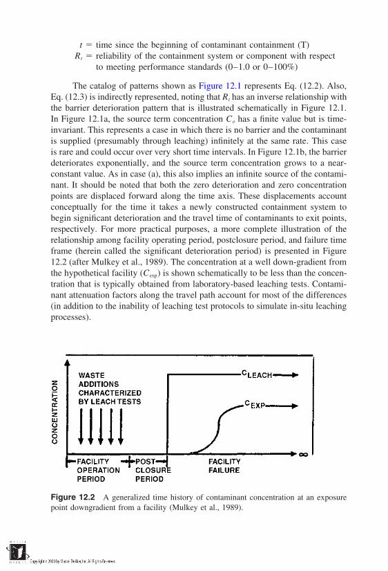
t time since the beginning of contaminant containment (T)Rt reliability of the containment system or component with respect

to meeting performance standards (0–1.0 or 0–100%)

The catalog of patterns shown as Figure 12.1 represents Eq. (12.2). Also,Eq. (12.3) is indirectly represented, noting that Rt has an inverse relationship withthe barrier deterioration pattern that is illustrated schematically in Figure 12.1.In Figure 12.1a, the source term concentration Co has a finite value but is time-invariant. This represents a case in which there is no barrier and the contaminantis supplied (presumably through leaching) infinitely at the same rate. This caseis rare and could occur over very short time intervals. In Figure 12.1b, the barrierdeteriorates exponentially, and the source term concentration grows to a near-constant value. As in case (a), this also implies an infinite source of the contami-nant. It should be noted that both the zero deterioration and zero concentrationpoints are displaced forward along the time axis. These displacements accountconceptually for the time it takes a newly constructed containment system tobegin significant deterioration and the travel time of contaminants to exit points,respectively. For more practical purposes, a more complete illustration of therelationship among facility operating period, postclosure period, and failure timeframe (herein called the significant deterioration period) is presented in Figure12.2 (after Mulkey et al., 1989). The concentration at a well down-gradient fromthe hypothetical facility (Cexp) is shown schematically to be less than the concen-tration that is typically obtained from laboratory-based leaching tests. Contami-nant attenuation factors along the travel path account for most of the differences(in addition to the inability of leaching test protocols to simulate in-situ leachingprocesses).

Figure 12.2 A generalized time history of contaminant concentration at an exposurepoint downgradient from a facility (Mulkey et al., 1989).

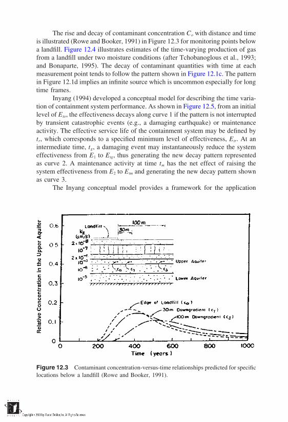
The rise and decay of contaminant concentration Co with distance and timeis illustrated (Rowe and Booker, 1991) in Figure 12.3 for monitoring points belowa landfill. Figure 12.4 illustrates estimates of the time-varying production of gasfrom a landfill under two moisture conditions (after Tchobanoglous et al., 1993;and Bonaparte, 1995). The decay of contaminant quantities with time at eachmeasurement point tends to follow the pattern shown in Figure 12.1c. The patternin Figure 12.1d implies an infinite source which is uncommon especially for longtime frames.

Inyang (1994) developed a conceptual model for describing the time varia-tion of containment system performance. As shown in Figure 12.5, from an initiallevel of Eto, the effectiveness decays along curve 1 if the pattern is not interruptedby transient catastrophic events (e.g., a damaging earthquake) or maintenanceactivity. The effective service life of the containment system may be defined bytr, which corresponds to a specified minimum level of effectiveness, Etr. At anintermediate time, tg, a damaging event may instantaneously reduce the systemeffectiveness from E1 to Etg, thus generating the new decay pattern representedas curve 2. A maintenance activity at time tm has the net effect of raising thesystem effectiveness from E2 to Etm and generating the new decay pattern shownas curve 3.

The Inyang conceptual model provides a framework for the application

Figure 12.3 Contaminant concentration-versus-time relationships predicted for specificlocations below a landfill (Rowe and Booker, 1991).

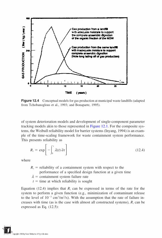
Figure 12.4 Conceptual models for gas production at municipal waste landfills (adaptedfrom Tchobanoglous et al., 1993; and Bonaparte, 1995).

of system deterioration models and development of single-component parametertracking models akin to those represented in Figure 12.1. For the composite sys-tems, the Weibull reliability model for barrier systems (Inyang, 1994) is an exam-ple of the time-scaling framework for waste containment system performance.This presents reliability as

Rt expt

0λ(t) ∂ t (12.4)

where

Rt reliability of a containment system with respect to theperformance of a specified design function at a given time

λ containment system failure ratet time at which reliability is sought

Equation (12.4) implies that Rt can be expressed in terms of the rate for thesystem to perform a given function (e.g., minimization of contaminant releaseto the level of 103 cm3/m2/s). With the assumption that the rate of failure in-creases with time (as is the case with almost all constructed systems), Rt can beexpressed as Eq. (12.5):

Figure 12.5 A Conceptual long-term deterioration pattern and maintenance scheme forwaste containment systems (Inyang, 1994).

Rt exp t to

n b

(12.5)

where

t0 location parameter time at the beginning of degradationb shape parameter (dimensionless)n scale parameter (dimensionless)

In order to match the reality that systems deteriorate with time, b musthave a positive value. Mathematically, b defines the geometry of the reliabilityversus-time curve and should range from 2.0 to 5.0 for containment systems. Thescale parameter n is the normalization factor for the time interval considered.Theoretically, it is a time duration that corresponds to

Ft 1 Rt 1 e1 0.632 (12.6)

Thus, to obtain n, the failure function of the containment system must be knownor estimated. From a plot of failure probability (Ft) versus time, the time value

Figure 12.6 A plot of composite reliability decay for a hypothetical nuclear waste re-pository using the Inyang Weibull model (Inyang, 1994).

that corresponds to Ft 0.632 is taken as n. Figure 12.6 shows plots of Rt fora hypothetical nuclear waste repository using b values of 2, 3, and 4, and an nvalue of 9000 years.

12.3 TYPES OF BARRIER MATERIALS

Several materials are used as barriers in waste containment systems. The criterionfor the selection of materials for each type of containment system can be one ormore of the following requirements:

Materials that have adequately high sorption capacityMaterials that can be compacted or cemented to high densities and effective

porosities that are low enough to minimize the flow of contaminantsthrough them

Materials that can react chemically with the contaminants that permeatethem, such that the concentrations of the contaminants are effectivelyreduced

Materials that can plug the pore spaces in natural soil such that large chan-nels for contaminant transport are effectively eliminated

In terms of chemical and mineralogical characteristics, barrier materials that per-form one or more of these functions fall into the categories described below.

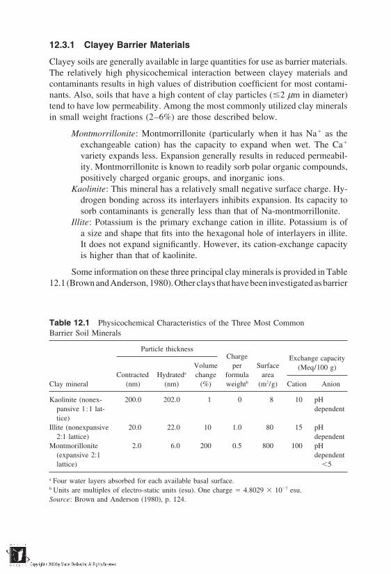
12.3.1 Clayey Barrier Materials

Clayey soils are generally available in large quantities for use as barrier materials.The relatively high physicochemical interaction between clayey materials andcontaminants results in high values of distribution coefficient for most contami-nants. Also, soils that have a high content of clay particles (2 µm in diameter)tend to have low permeability. Among the most commonly utilized clay mineralsin small weight fractions (2–6%) are those described below.

Montmorrillonite: Montmorrillonite (particularly when it has Na as theexchangeable cation) has the capacity to expand when wet. The Ca

variety expands less. Expansion generally results in reduced permeabil-ity. Montmorrillonite is known to readily sorb polar organic compounds,positively charged organic groups, and inorganic ions.

Kaolinite: This mineral has a relatively small negative surface charge. Hy-drogen bonding across its interlayers inhibits expansion. Its capacity tosorb contaminants is generally less than that of Na-montmorrillonite.

Illite: Potassium is the primary exchange cation in illite. Potassium is ofa size and shape that fits into the hexagonal hole of interlayers in illite.It does not expand significantly. However, its cation-exchange capacityis higher than that of kaolinite.

Some information on these three principal clay minerals is provided in Table12.1 (Brown andAnderson, 1980).Other clays thathave been investigated asbarrier

Table 12.1 Physicochemical Characteristics of the Three Most CommonBarrier Soil Minerals

Particle thicknessCharge Exchange capacity

Volume per Surface (Meq/100 g)Contracted Hydrateda change formula area

Clay mineral (nm) (nm) (%) weightb (m2/g) Cation Anion

Kaolinite (nonex- 200.0 202.0 1 0 8 10 pHpansive 1:1 lat- dependenttice)

Illite (nonexpansive 20.0 22.0 10 1.0 80 15 pH2:1 lattice) dependent

Montmorillonite 2.0 6.0 200 0.5 800 100 pH(expansive 2:1 dependentlattice) 5

a Four water layers absorbed for each available basal surface.b Units are multiples of electro-static units (esu). One charge 4.8029 107 esu.Source: Brown and Anderson (1980), p. 124.

materials are attapulgite and vermiculite. Clays are commonly used mix compo-nents of covers, liners, and slurry walls. Often, they are mixed with silts and sands.

12.3.2 Mineral Oxides, Organics, and Polymer Liquids

Several oxides exhibit high sorption and reactive capacities for both organic andinorganic contaminants. Mineral oxides such as zero-valent iron (Fe0), hematite,fly ash, and geothite are usually utilized as additives to clayey materials. Fe0 isthe most common material used in permeable reactive barriers for chlorinatedorganic compounds. Organics and cementitious materials are used as grouts, ex-amples of which are summarized in Table 12.2.

12.3.3 Polymeric Membranes

Membranes are used as barrier materials in impoundment/landfill liners, covers,and slurry walls. They lack the contaminant attenuation capacity of clays andminerals, but they have higher containment capacity for vapors. Their flexibilitymakes it possible to maintain the waste containment function under moderatedeformation conditions. Additives such as carbon black, pigments, fillers, plasti-cizers, processing aids, cross-linking chemicals, antidegradants, and biocides areusually combined with raw polymers to produce a variety of polymeric sheets.The majority of polymeric materials used in waste containment systems are pre-

Table 12.2 Some Key Properties of Barrier Additives and Chemical Grouts

Hydraulic Resistance Resistance Expectedconductivity Resistance to to lifetime

Grout (cm/s) to acids bases organics (years)

Sodium silicate 105 Fair Poor Fair 10–20Acrylate gels 107–109 Poor Good Fair 10–20Colloidal silica 108 Good Poor Good 25Iron hydroxide 107 Poor Good Good 25Montan wax 104–107 Fair Fair Fair 25Sulfur polymer 1010 Good Poor Fair 25

cementEpoxy 1010 Good Good Good 25Polysiloxane 1010 Good Good Good 25Furan 108–1010 Good Good Good 25Polyester styrene 1010 Good Good Fair 25Vinylester styrene 1010 Good Good Good 25Acrylics 109–1011 Good Good Good 25

Source: Whang and Committee, (1995).

sented in Table 12.3. Also, their compositions are summarized in Table 12.4(after Haxo et al., 1985). The characteristics of each of the polymers listed, in-cluding their durability factors are discussed in detail by the U.S. EPA (1980).

12.3.4 Geosynthetic-Clay Materials

Geosynthetic-clay liner materials are composites of sodium bentonite in layersof geosynthetics. The geosynthetic layers are sewn such that bentonite is sand-wiched among them. The composite material performs better than either compo-nent (Daniel and Koerner, 1993). Essentially, the geosynthetics provide increasedcrack resistance under differential settlement and cycles of wetting/drying andfreezing and thawing. The clay material swells in contact with moisture suchthat permeability is low. It also provides contaminant attenuation capacity to thecomposite material.

Table 12.3 Polymeric Materials Used in Liners

Type of Thickness FabricPolymer Abbreviation compounda (mm) reinforced

Butyl rubber IIR XL 0.9–2.3 Yes, noChlorinated polyethylene CPE TP 0.5–1.0 Yes, noChlorosulfonated

polyethylene CSPE TP,XL 0.6–1.0 Yes, noElasticized polyolefin ELPO CX 0.6 NoElasticized polyvinyl

chloride PVC-E TP 0.8–0.9 YesEpichlorohydrin rubber ECO XL 1.67 Yes, noEthylene propylene

rubber EPDM XL, TP 0.5–1.6 Yes, noNeoprene CR XL 0.5–1.8 Yes, noNitrile rubber NBR XL 0.8 YesPolyester elastomer PEEL CX 0.18 NoPolyethylene

Low-density LDPE CX 0.3–0.8 NoLinear low-density LLDPE CX 0.5–0.8 NoHigh-density HDPE CX 0.5–3.1 No

Polyvinyl chloride PVC TP 0.3–0.9 Yes, noPolyvinyl chloride,

oil resistant PVC-OR TP 0.8 Yes, noThermoplastic elastomer TPE CS 1.0 No

a TP thermoplastic; CX partially crystalline; XL cross-linked.Source: Haxo et al. (1985).

Table 12.4 Basic Compositions of Polymeric Membrane Liner Compounds

Composition of compound type, parts by weight

Component Cross-linked Thermoplastic Crystalline

Polymer or alloy 100 100 100Oil or plasticizer 5–40 5–55 0–10Fillers:

Carbon black 5–40 5–40 2–5Inorganics 5–40 5–40 —

Antidegradants 1–2 1 1Cross-linking system:

Inorganic 5–9 a —Sulfur 5–9 — —

a An inorganic curing system that cross-links over time is incorporated in CSPE liner compounds.Source: Haxo et al. (1985).

12.3.5 Other Barrier Materials

Other materials used in various waste containment system configurations includePortland cement concrete, paper mill sludges (Moo-Young and Zimmie, 1995),coal combustion flyash (Sarsby and Finch, 1995; Fleming and Inyang, 1995);limestone (Artiola and Fuller, 1980); slags (Khera, 1995); and organobentonites(Smith and Li, 1995). Evans et al. (1990) have summarized experiences withzeolites, organically modified clays, flyash, bentonite, and natural clay in compos-ite liners for waste containment.

12.4 MATERIAL DETERIORATION MECHANISMS

It is important to distinguish between material deterioration, which depends onthe durability of the material, among other factors, and the deterioration of acontainment system that comprises the material. Material deterioration analysisfocuses on the physicochemical characteristics of the material and how theychange with time in response to environmental conditions. The dimensions ofthe component that comprises the material, and the overall configuration ofthe containment system are usually not factored into expressions of material dura-bility or deterioration. System deterioration or degradation covers both materialdurability and interactions among the components of the overall system. Thisrequires consideration of component dimensions and system configuration aswell.

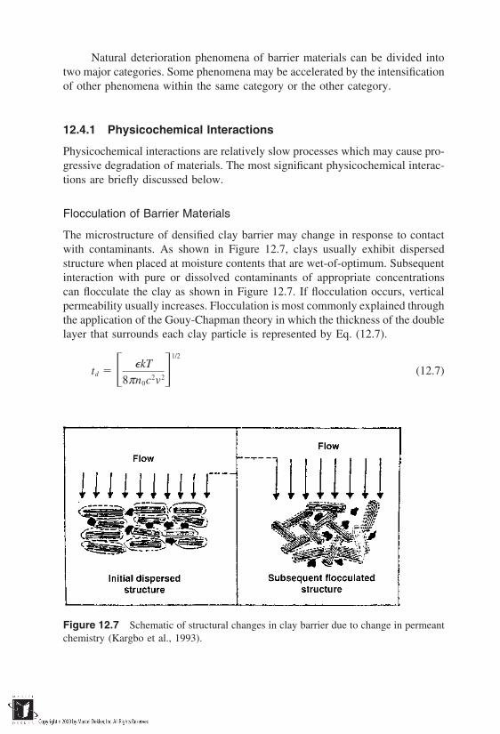
Natural deterioration phenomena of barrier materials can be divided intotwo major categories. Some phenomena may be accelerated by the intensificationof other phenomena within the same category or the other category.

12.4.1 Physicochemical Interactions

Physicochemical interactions are relatively slow processes which may cause pro-gressive degradation of materials. The most significant physicochemical interac-tions are briefly discussed below.

Flocculation of Barrier Materials

The microstructure of densified clay barrier may change in response to contactwith contaminants. As shown in Figure 12.7, clays usually exhibit dispersedstructure when placed at moisture contents that are wet-of-optimum. Subsequentinteraction with pure or dissolved contaminants of appropriate concentrationscan flocculate the clay as shown in Figure 12.7. If flocculation occurs, verticalpermeability usually increases. Flocculation is most commonly explained throughthe application of the Gouy-Chapman theory in which the thickness of the doublelayer that surrounds each clay particle is represented by Eq. (12.7).

td kT

8πn0c2v21/2

(12.7)

Figure 12.7 Schematic of structural changes in clay barrier due to change in permeantchemistry (Kargbo et al., 1993).

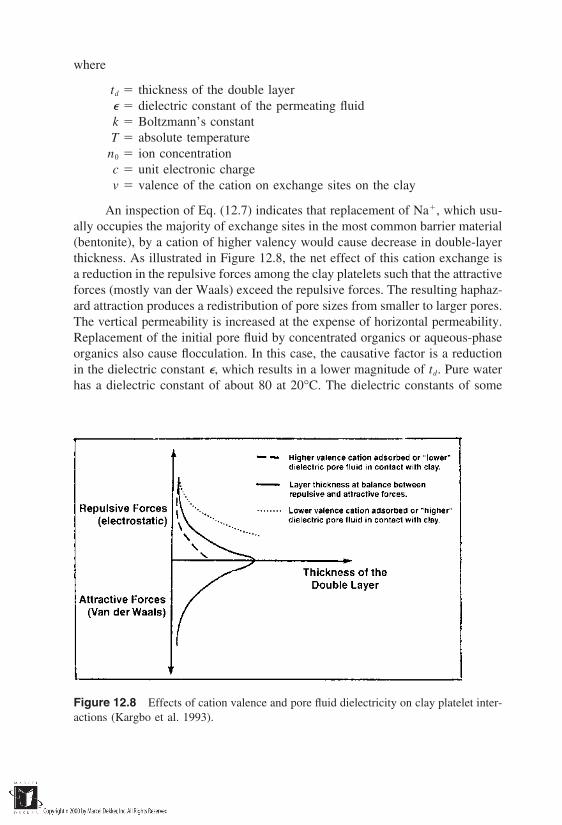
where

td thickness of the double layer dielectric constant of the permeating fluidk Boltzmann’s constantT absolute temperature

n0 ion concentrationc unit electronic chargev valence of the cation on exchange sites on the clay

An inspection of Eq. (12.7) indicates that replacement of Na, which usu-ally occupies the majority of exchange sites in the most common barrier material(bentonite), by a cation of higher valency would cause decrease in double-layerthickness. As illustrated in Figure 12.8, the net effect of this cation exchange isa reduction in the repulsive forces among the clay platelets such that the attractiveforces (mostly van der Waals) exceed the repulsive forces. The resulting haphaz-ard attraction produces a redistribution of pore sizes from smaller to larger pores.The vertical permeability is increased at the expense of horizontal permeability.Replacement of the initial pore fluid by concentrated organics or aqueous-phaseorganics also cause flocculation. In this case, the causative factor is a reductionin the dielectric constant , which results in a lower magnitude of td. Pure waterhas a dielectric constant of about 80 at 20°C. The dielectric constants of some

Figure 12.8 Effects of cation valence and pore fluid dielectricity on clay platelet inter-actions (Kargbo et al. 1993).

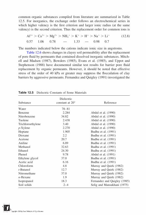
common organic substances compiled from literature are summarized in Table12.5. For inorganics, the exchange order follows an electrochemical series inwhich higher valency is the first criterion and larger ionic radius (at the samevalency) is the second criterion. Thus the replacement order for common ions is

Al3 Ca2 Mg2 NH4 K H Na Li (12.8)

0.57 1.06 0.78 — 1.33 — 0.98 0.7

The numbers indicated below the cations indicate ionic size in angstroms.Table 12.6 shows changes in clayey soil permeability after the replacement

of pore fluid by permeants that contained dissolved inorganic substances. Mitch-ell and Madsen (1987), Bowders (1985), Evans et al. (1985), and Uppot andStephenson (1988) have documented similar test results for barrier pore fluidreplacement by organic permeants. However, it should be noted that effectivestress of the order of 40 kPa or greater may suppress the flocculation of claybarriers by aggressive permeants. Fernandez and Quigley (1991) investigated the

Table 12.5 Dielectric Constants of Some Materials

DielectricSubstance constant at 20° Reference

Water 78–81Benzene 2.284 Abdul et al. (1990)Nitrobenzene 34.82 Abdul et al. (1990)Tuolene 2.438 Abdul et al. (1990)Trichloroethylene 3.40 Abdul et al. (1990)p-Xylene 2.270 Abdul et al. (1990)Heptane 1.905 Budhu et al. (1991)Dioxane 2.2 Budhu et al. (1991)Acetone 20.7 Budhu et al. (1991)Aniline 6.89 Budhu et al. (1991)Methanol 32.63 Budhu et al. (1991)Ethanol 24.30 Budhu et al. (1991)Phenol 9.78 Abdul et al. (1991)Ethylene glycol 37.0 Budhu et al. (1991)Acetic acid 6.16 Budhu et al. (1991)Chloroform 4.8 Murray and Quirk (1982)t-Butanol 12.7 Murray and Quirk (1982)Nitromethane 37.0 Murray and Quirk (1982)n-Hexane 1.9 Murray and Quirk (1982)Isopropanol 18.3 Fernandez and Quigley (1985)Soil solids 2–4 Selig and Mansukhani (1975)

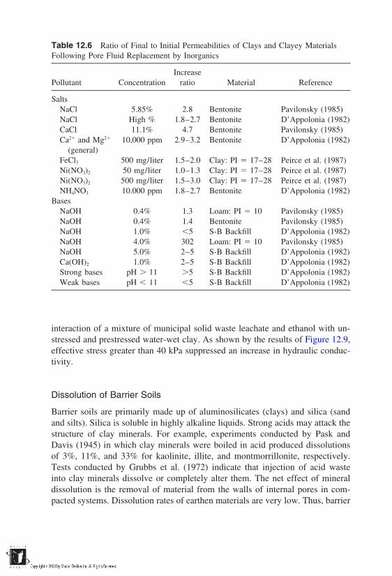
Table 12.6 Ratio of Final to Initial Permeabilities of Clays and Clayey MaterialsFollowing Pore Fluid Replacement by Inorganics

IncreasePollutant Concentration ratio Material Reference

SaltsNaCl 5.85% 2.8 Bentonite Pavilonsky (1985)NaCl High % 1.8–2.7 Bentonite D’Appolonia (1982)CaCl 11.1% 4.7 Bentonite Pavilonsky (1985)Ca2 and Mg2 10,000 ppm 2.9–3.2 Bentonite D’Appolonia (1982)

(general)FeCl3 500 mg/liter 1.5–2.0 Clay: PI 17–28 Peirce et al. (1987)Ni(NO3)2 50 mg/liter 1.0–1.3 Clay: PI 17–28 Peirce et al. (1987)Ni(NO3)2 500 mg/liter 1.5–3.0 Clay: PI 17–28 Peirce et al. (1987)NH4NO3 10.000 ppm 1.8–2.7 Bentonite D’Appolonia (1982)

BasesNaOH 0.4% 1.3 Loam: PI 10 Pavilonsky (1985)NaOH 0.4% 1.4 Bentonite Pavilonsky (1985)NaOH 1.0% 5 S-B Backfill D’Appolonia (1982)NaOH 4.0% 302 Loam: PI 10 Pavilonsky (1985)NaOH 5.0% 2–5 S-B Backfill D’Appolonia (1982)Ca(OH)2 1.0% 2–5 S-B Backfill D’Appolonia (1982)Strong bases pH 11 5 S-B Backfill D’Appolonia (1982)Weak bases pH 11 5 S-B Backfill D’Appolonia (1982)

interaction of a mixture of municipal solid waste leachate and ethanol with un-stressed and prestressed water-wet clay. As shown by the results of Figure 12.9,effective stress greater than 40 kPa suppressed an increase in hydraulic conduc-tivity.

Dissolution of Barrier Soils

Barrier soils are primarily made up of aluminosilicates (clays) and silica (sandand silts). Silica is soluble in highly alkaline liquids. Strong acids may attack thestructure of clay minerals. For example, experiments conducted by Pask andDavis (1945) in which clay minerals were boiled in acid produced dissolutionsof 3%, 11%, and 33% for kaolinite, illite, and montmorrillonite, respectively.Tests conducted by Grubbs et al. (1972) indicate that injection of acid wasteinto clay minerals dissolve or completely alter them. The net effect of mineraldissolution is the removal of material from the walls of internal pores in com-pacted systems. Dissolution rates of earthen materials are very low. Thus, barrier

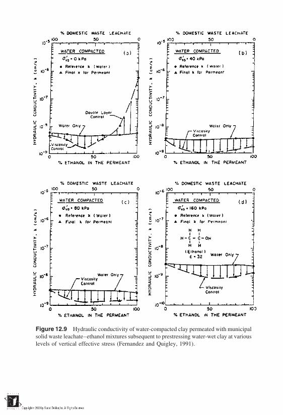
Figure 12.9 Hydraulic conductivity of water-compacted clay permeated with municipalsolid waste leachate–ethanol mixtures subsequent to prestressing water-wet clay at variouslevels of vertical effective stress (Fernandez and Quigley, 1991).

materials require very long residence times of an aggressive liquid to dissolvesignificantly.

Cracking of Densified Barrier Materials

Cracking can be caused by a variety of stress-inducing phenomena. Among suchphenomena are desiccation, cycles of heating and coaling, wetting and dryingand freezing and thawing, geostatic and geodynamic loading, and even chemicalattack. The propensity of barrier materials to crack is higher near the groundsurface, where thermal, moisture, and other gradients are higher in magnitudeand frequency. Fang (1994) developed a time-distribution scheme for varioustypes of cracks in geomedia. As shown in Figure 12.10, the scheme identifiesshrinkage, thermal loading, and loading as the initial set of stressors that producecracks. During an intermediate stage called the degradation stage, the fracturesgrow dramatically. Crack growth is exponential, such that a limiting crackingstage which defines the useful life of the material or system is soon attained.Beyond this stage, the material is considered to be in a state of failure. In coldregions, cracks can be initiated and extended in barrier materials by freeze/thaw

Figure 12.10 Schematic diagram illustrating the crack–time relationship at variouscracking stages (Fang, 1994).

cycles. Figure 12.11 shows the effects of freeze/thaw cycles on the permeabilitiesof four compacted clays. The permeability tends to increase dramatically withinthe first 1–4 cycles. Thereafter, increase in permeability is less significant. Appar-ently, textural changes in soil are more difficult to achieve after the initial clog-ging of larger pores.

Exposed Slope Failures by Creep

Some containment systems, such as landfills and waste piles, have componentsthat have exposed slopes. Much attention has been paid to the reliability of suchslopes. The reliability of a landfill slope or any component of the landfill shouldbe distinguished from the reliability of the entire landfill (a composite system).With respect to the deterioration of materials that make up a landfill slope, thesoil may deform progressively under its weight or imposed stresses until the slopefails.

For cover systems, unconfined compressive strength is the most commonstrength parameter used in soil material performance assessment. As an earlydevelopment in soil mechanics, Casagrande and Wilson (1951) conducted creep

Figure 12.11 Summary of freeze/thaw permeability test results for four compactedclays (Chamberlain et al., 1990).

tests to assess the long-term unconfined compressive strength of clays and clayshales at constant moisture content. In general, the following equation can beused to express the rate of strength decrease with time in their tests:

σ t σa σo logt

ta

σa 1 ρa logt

ta (12.9)

where

σ t unconfined strength of saturated soils (F/L2)σo decrease in strength for logarithmic time cycle (F/L2)ρa coefficient of rheological decrease in strength σo/σa

(dimensionless fraction)σa reference (set initial) strength (F/L2)ta reference (set initial) time (T)t time in the future for which strength is sought (T)

If ta is fixed at 1000 min, the envelop of magnitudes for σa is about 0.05–0.15. Closely related to the deterioration of cover slopes of containment systemsis the increased potential of interface failures as moisture accumulates and drainsdownward at the earthen material/polymeric sheet interface. The lubricating ef-fect could reduce interface friction such that portions of the cover fail.

Deterioration of Polymeric Materials

Sustained exposure to sunlight (ultraviolet radiation), chemicals, high tempera-tures, and cycles of these and other stresses can reduce the strength and generatepotential flow channels in polymeric materials. An Arhenius-type model is com-monly used to estimate the rate constant for the deterioration of polymeric materi-als using data from laboratory-based accelerated aging tests. The most significantmolecular-level chemical attack processes on geomembranes (Koerner and Rich-ardson, 1987) are breaking of carbon–carbon bonds (metathesis); breaking ofcarbon–non-carbon bonds in the amorphous phase (solvolysis); loss of electronsto oxygen by molecular constituents of the polymeric material (oxidation); anddissolution of the polymer, often preceded by swelling.

Polymer oxidation is enhanced by the release of a free radical. As explainedby Koerner et al. (1990), the free radical can combine with oxygen to form ahydroperoxy radical which traverses the molecular structure of the polymer andreacts with other units. More radicals are released such that these oxidative reac-tions are intensified. This chain reaction is represented by Eqs. (12.10) and(12.11).

R• O2 → ROO• (12.10)

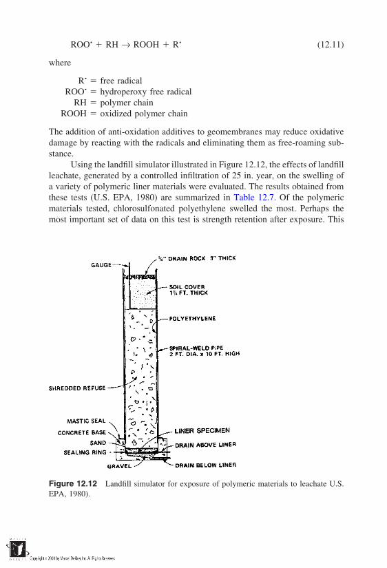
ROO• RH → ROOH R• (12.11)

where

R• free radicalROO• hydroperoxy free radical

RH polymer chainROOH oxidized polymer chain

The addition of anti-oxidation additives to geomembranes may reduce oxidativedamage by reacting with the radicals and eliminating them as free-roaming sub-stance.

Using the landfill simulator illustrated in Figure 12.12, the effects of landfillleachate, generated by a controlled infiltration of 25 in. year, on the swelling ofa variety of polymeric liner materials were evaluated. The results obtained fromthese tests (U.S. EPA, 1980) are summarized in Table 12.7. Of the polymericmaterials tested, chlorosulfonated polyethylene swelled the most. Perhaps themost important set of data on this test is strength retention after exposure. This

Figure 12.12 Landfill simulator for exposure of polymeric materials to leachate U.S.EPA, 1980).

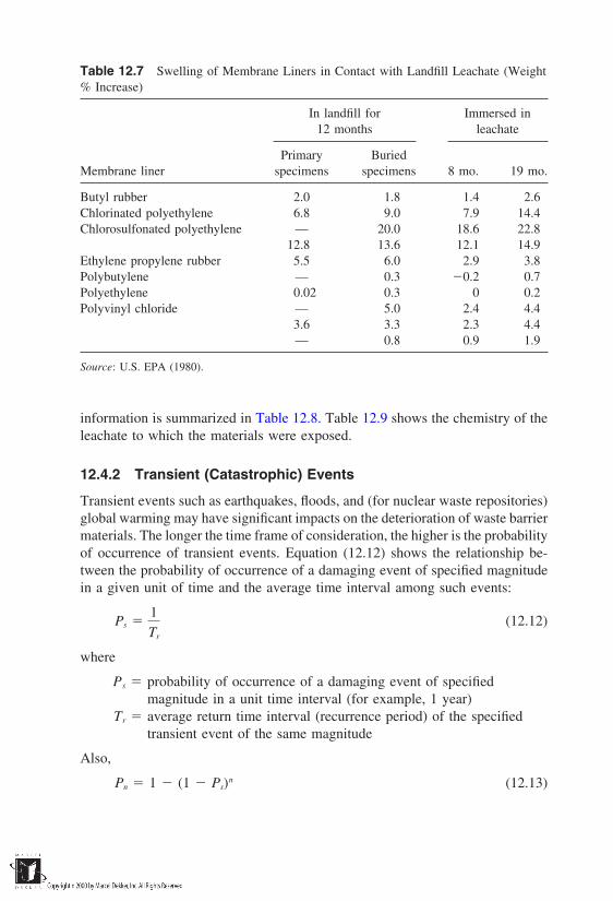
Table 12.7 Swelling of Membrane Liners in Contact with Landfill Leachate (Weight% Increase)

In landfill for Immersed in12 months leachate

Primary BuriedMembrane liner specimens specimens 8 mo. 19 mo.

Butyl rubber 2.0 1.8 1.4 2.6Chlorinated polyethylene 6.8 9.0 7.9 14.4Chlorosulfonated polyethylene — 20.0 18.6 22.8

12.8 13.6 12.1 14.9Ethylene propylene rubber 5.5 6.0 2.9 3.8Polybutylene — 0.3 0.2 0.7Polyethylene 0.02 0.3 0 0.2Polyvinyl chloride — 5.0 2.4 4.4

3.6 3.3 2.3 4.4— 0.8 0.9 1.9

Source: U.S. EPA (1980).

information is summarized in Table 12.8. Table 12.9 shows the chemistry of theleachate to which the materials were exposed.

12.4.2 Transient (Catastrophic) Events

Transient events such as earthquakes, floods, and (for nuclear waste repositories)global warming may have significant impacts on the deterioration of waste barriermaterials. The longer the time frame of consideration, the higher is the probabilityof occurrence of transient events. Equation (12.12) shows the relationship be-tween the probability of occurrence of a damaging event of specified magnitudein a given unit of time and the average time interval among such events:

Ps 1Tr

(12.12)

where

Ps probability of occurrence of a damaging event of specifiedmagnitude in a unit time interval (for example, 1 year)

Tr average return time interval (recurrence period) of the specifiedtransient event of the same magnitude

Also,

Pn 1 (1 Ps)n (12.13)

Table 12.8 Retention Modulus of Polymeric Membrane Liner Materials onImmersion in Landfill Leachatea

Retention % ofS-200, psi original value

LinerPolymer no. Unexposed 8 mo. 19 mo. 8 mo. 19 mo.

Butyl rubber 44 685 590 620 86 90Chlorinated polyethylene 12 1330 1130 1190 89 89

38 1205 1070 1090 89 9086 810 790 860 98 106

Chlorosulfonated polyethylene 3 735 395 335 54 460b 1550 1775 2070 114 134

85 1770 1360 1920 77 108Elasticized polyolefin 36 970 1005 1050 104 109Ethylene propylene rubber 8 690 870 860 126 124

18 760 840 830 110 10983b 845 905 900 107 10791 855 775 790 91 9241 1040 1035 1030 100 99

Neoprene 9 1235 975 950 79 7737 1635 1630 1640 100 10042b — — — — —90 1190 1245 1350 105 114

Polybutylene 98 3120 3160 3150 101 101Polyester elastomer 75 2735 2790 2670 102 98Polyethylene 21 1260 1340 1285 106 102Polyvinyl chloride 11 2120 1845 1805 87 85

17 1965 1570 1640 80 8419 1740 1545 1645 89 9440 1720 1560 1570 91 9167 1700 1570 1780 92 10588 2400 1900 2105 79 8889 2455 2370 2330 96 95

Polyvinyl chloride pitchc 52 1020 870 880 85 86

a Average of stress at 200% elongation (S-200) measured in machine and transverse directions.b Fabric reinforced.c S-100 values given; original and subsequent exposed specimens failed at less than 200% elongation.Source: U.S. EPA (1980).

where

Pn probability of occurrence of the specified event during anextended time interval

n extended time interval for which the analysis is conducted

As discussed in Sections 12.1 and 12.2, most containment systems com-prise many components, each of which is susceptible to different degrees of

Table 12.9 Chemistry of Leachate Used to TestPolymeric Membrane Materialsa

Test Value

Total solids, % 3.31Volatile solids, % 1.95Nonvolatile solids, % 1.36

Chemical oxygen demand (COD), g/liter 45.9pH 5.05Total volatile acids (TVA), g/liter 24.33Organic acids, g/liter

Acetic 11.25Propionic 2.87Isobutyric 0.81Butyric 6.93

a At the end of the first year of operation when the first set ofliner specimens were recovered.

Source: U.S. EPA (1980).

stresses that can be imposed by transient events. Thus, the expression for thecomposite system must account for the composite nature of the system and theconditional probability of failure of each component. The relevant general expres-sion for a case in which the failure of a component is tantamount to the failureof the system is given by Eq. (12.14).

Pc Pn[P( f/o)a P( f/o)b---------P( f/o)k] (12.14)

where

Pc probability of failure of a containment system given thatthe design transient event has the probability Pn ofoccurrence during the considered time duration

P( f/o) i conditional probability that a specific component, i, of thesystem will fail, given the occurrence of the designtransient event (i a, b, --- k).

Tr can be obtained from historical data such as seismic intensity recordsand flood history. For example, Bollinger (1976) observed that for earthquakeintensities ranging from V to VIII for the southeastern United States, the relation-ship expressed as Eq. (12.15) can be used to estimate Tr. Obviously, this equation,like all correlation equations, may require updating because, as more earthquakesoccur, the correlative relationship may change.

log(1/Tr) 3.01 0.59Io (12.15)

Figure 12.13 Illustration of the deformation of the components of a landfill by seismicactivity (Inyang, 1992).

where Io earthquake intensity and Tr is, as previously defined, measured inyears. Computation of P( f/o) i for real systems requires stability or fluid flowanalysis of each of the components of the system. Methods for such analysesare described briefly in Chapter 11 of this text and in more detail in traditionalgeotechnical engineering texts. The definition of failure state for a componentof the system [which is a requirement for the quantification of P( f/o) i] is proneto confusion because functional failure and structural failure may not occur con-currently, at least initially. An example of the development of flaws in a contain-ment system due to a transient event is illustrated in Figure 12.13 (Inyang, 1992)for a landfill impacted by seismic forces. The generation of flaws may result inacceleration of barrier material degradation.

12.5 SYSTEM PERFORMANCE MONITORINGTECHNIQUES

Containment system monitoring techniques can be classified on the basis of tech-nology or approach. The utilities of monitoring techniques with respect to eachof the classifications are summarized in Table 12.10. There are three types ofapproaches to containment system performance monitoring: external barrier in-tegrity monitoring, barrier permeation monitoring, and functional monitoring.

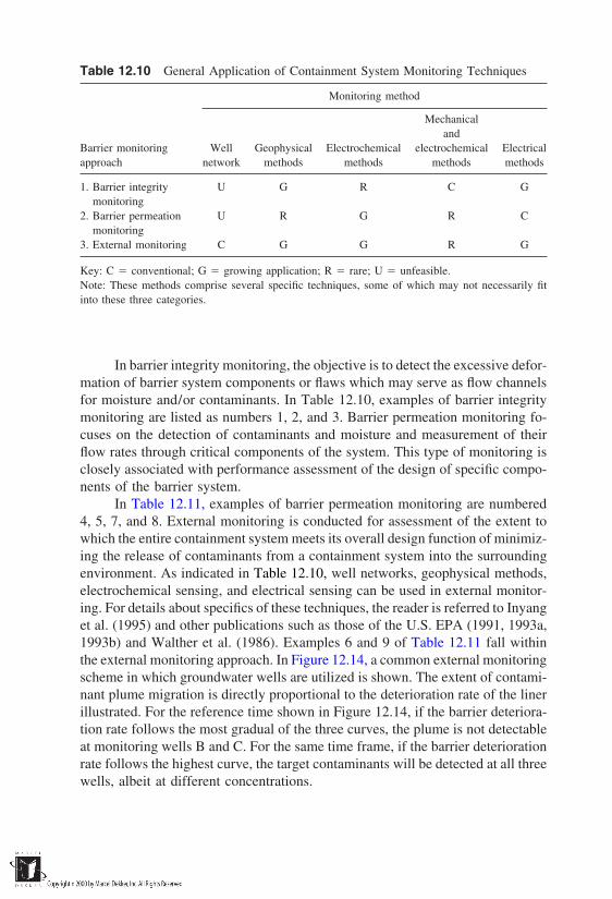
Table 12.10 General Application of Containment System Monitoring Techniques

Monitoring method

Mechanicaland

Barrier monitoring Well Geophysical Electrochemical electrochemical Electricalapproach network methods methods methods methods

1. Barrier integrity U G R C Gmonitoring

2. Barrier permeation U R G R Cmonitoring

3. External monitoring C G G R G

Key: C conventional; G growing application; R rare; U unfeasible.Note: These methods comprise several specific techniques, some of which may not necessarily fitinto these three categories.

In barrier integrity monitoring, the objective is to detect the excessive defor-mation of barrier system components or flaws which may serve as flow channelsfor moisture and/or contaminants. In Table 12.10, examples of barrier integritymonitoring are listed as numbers 1, 2, and 3. Barrier permeation monitoring fo-cuses on the detection of contaminants and moisture and measurement of theirflow rates through critical components of the system. This type of monitoring isclosely associated with performance assessment of the design of specific compo-nents of the barrier system.

In Table 12.11, examples of barrier permeation monitoring are numbered4, 5, 7, and 8. External monitoring is conducted for assessment of the extent towhich the entire containment system meets its overall design function of minimiz-ing the release of contaminants from a containment system into the surroundingenvironment. As indicated in Table 12.10, well networks, geophysical methods,electrochemical sensing, and electrical sensing can be used in external monitor-ing. For details about specifics of these techniques, the reader is referred to Inyanget al. (1995) and other publications such as those of the U.S. EPA (1991, 1993a,1993b) and Walther et al. (1986). Examples 6 and 9 of Table 12.11 fall withinthe external monitoring approach. In Figure 12.14, a common external monitoringscheme in which groundwater wells are utilized is shown. The extent of contami-nant plume migration is directly proportional to the deterioration rate of the linerillustrated. For the reference time shown in Figure 12.14, if the barrier deteriora-tion rate follows the most gradual of the three curves, the plume is not detectableat monitoring wells B and C. For the same time frame, if the barrier deteriorationrate follows the highest curve, the target contaminants will be detected at all threewells, albeit at different concentrations.

Table 12.11 Examples of Traditional and Innovative Monitoring Techniques for Specific Waste Containment Problems

Waste containment problem Monitoring techniques

1. Cover slope deformation and failure Inclinometers, electrical resistance shear strips, and vibratingwire extensiometers

2. Lateral deformation of vertical walls Electrical inclinometers, extensiometers, and tiltmeters3. Excessive settlement and cracking of soil and concrete covers Sealed Borros anchor, inclinometers, settlement platforms, elec-

trical crack guages, convergence gauges, microwave sensors,dye-tracing

4. Excessive infiltration of cover systems Tensiometers, gypsum blocks, psychrometers, neutron gaugesand piezometers in covers, thermoelectric flow velocitygauges in drainage layers, and fiber-optic moisture sensors incovers

5. Voids and high permeability zones in emplaced and natural Crosshole seismic surveys, ground-penetrating radar surveys,barriers seismic tomography, surface-based seismic refraction surveys,

soil gas surveys, temperature logging, cone penetration test-ing, and dye tracing

6. Leachate plume migration from waste containment systems; and Electrochemical sensing cables and fiber-optic containmentplume capture by permeable reactive walls structure, DC electrical and electromagnetic resistance sur-

veys above ground, ground-penetrating radar surveys, dye-tracing, and groundwater monitoring

7. Contaminant flow through bottom barriers and low-hydraulic Electrochemical sensing cables and fiber-optic chemical sensorsconductivity walls within, upgradient, and downgradient from barriers, and

pumping tests8. Leaks in geomembranes and sheet pile joints Electrical leak detection systems and fiberoptic monitoring sys-

tems for joints9. Flow of leachate through reactive, permeable walls Thermal flow sensors upstream, within, and downstream from

wall, electrochemical sensors, pH and Eh sensors

Figure 12.14 Relationship among barrier deterioration rate, extent of contaminantplume migration, and plume detection at monitoring wells.

REFERENCES

Abdul, A. S., Gibson, T. L., and Rai, D. N. (1990). Laboratory studies of flow of someorganic solvents and their aqueous solutions through bentonite and kaolin clays.Ground Water, 28(4):524–533.

Artiola, J., and Fuller, W. H. (1980). Limestone liner for landfill leachates containingberyllium, cadmium, iron, nickel and zinc. Soil Sci., 129(3):167–179.

Bollinger, G. A. (1976). The seismic regime in a minor earthquake zone. Proc. ASCEConf. on Numerical Methods in Geomechanics, 11:917–937.

Bonaparte, R. 1995. Long-term performance of landfills. Proc. Conf. (Geoenvironment2000) on Characterization, Containment, Remediation and Performance in Envi-ronmental Geotechnics, American Society of Civil Engineers, New Orleans, LA,pp. 514–553.

Bowders, J. J. (1985). The influence of various concentrations of organic liquids on theconductivity of compacted clay. Geotechnical Engineering Dissertation GT85-2,University of Texas, Austin.

Brown, K. W., and Anderson, D. (1980). Effect of organic chemicals on clay liner perme-ability. Proc. 6th Annual Research Symp. EPA-600/0-80-010. U.S. EnvironmentalProtection Agency, Cincinnati, OH, pp. 123–134.

Budhu, M., Giese, R. F., Campbell, G., and Baumgrass, L. (1991). The permeability ofsoils with organic fluids. Can. Geotech. J., 28:140–147.

Casagrande, A., and Wilson, S. D. (1951). Effect of rate of loading on the strength ofclays and shales at constant water content. Geotechnique, 2:251–263.

Chamberlain, E. J., Iskandar, I. and Hunsicker, S. E. (1990). Effect of freeze-thaw cycleson the permeability and macrostructure of soils. Proc. Conf. on Frozen Soil Impactson Agriculture, Range and Forest Lands, Spokane, WA, pp. 145–155.

Daniel, D. E., and Koerner, R. M. (1993). Cover systems. In: Geotechnical Practice forWaste Disposal, D. E., Daniel, ed. Chapman and Hall, New York, pp. 455–496.

D’Appolonia, D. J. (1982). Slurry trench cut-off walls of hazardous waste isolation. Proc.13th Annual Geotechnical Lecture Series, Geotechnical Group, ASCE, Philadel-phia.

Evans, J. C., Fang, H. Y., and Kugelman, I. J. (1985). Organic fluid effects on the perme-ability of soil-bentonite slurry walls. Proc. Natl. Conf. on Hazardous Wastes andEnvironmental Emergencies, Cincinnati, OH.

Evans, J. C., Sambasivam, Y., and Zarlinski, S. (1990). Attenuating materials in compositeliners. Proc. Symp. on Waste Containment Systems Held in Conjunction with theNational Convention of the American Society of Civil Engineers, San Francisco,CA, pp. 247–263.

Fang, H. Y. (1994). Cracking and fracture characteristics of contaminated fine-grainedsoil. Material developed for presentation at a Session on Application of FractureMechanics to Geotechnical Engineering, Annual Convention of the American Soci-ety of Civil Engineers, Atlanta, GA.

Fernandez, F., and Quigley, R. M. (1985). Hydraulic conductivity of natural clays perme-ated with simple liquid hydrocarbons. Can. Geotech. J., 22:205–214.

Fernandez, F., and Quigley, R. M. (1991). Controlling the destructive effects of clay-organic liquid interactions by application of effective stresses. Can. Geotech. J.,28:388–398.

Fleming, L. N., and Inyang, H. I. (1995). Permeability of clay-modified fly ash underthermal gradients. J. Mater. in Civil Eng., ASCE, 7(3):178–182.

Grubbs, D. M., Haynes, C. D., Hughes, T. H., and Stow, S. H. (1972). Compatibility ofsubsurface reservoirs with injected liquid wastes, Report no. 721. Natural ResourcesCenter, University of Alabama, Huntsville, Alabama.

Haxo, H. E., Nelson, N. A., and Miedema, J. A. (1985). Solubility parameters for pre-dicting membrane-waste liquid compatibility. Proc. 11th Annual Research Symp.EPA/600/9-85/013. U.S. Environmental Protection Agency, Washington, DC,pp. 198–212.

Inyang, H. I. (1992). Aspects of landfill design for stability in seismic zones. J. Environ.Syst., 21(3):223–235.

Inyang, H. I. (1994). A Weibull-based reliability analysis of waste containment systems.Proc. First Int. Congress on Environmental Geotechnics, Alberta, Canada, pp. 273–278.

Inyang, H. I., Betsill, J. D., Breeden, R., Chamberlain, G. H., Dutta, S., Everett, L., Fuen-tes, R., Hendrickson, J., Koutsandreas, J., Lesmes, D., Loomis, G., Mangion, S. M.,Morgan, D., Pfeifer, C., Puls, R. W., Stamnes, R. L., Vandel, T. D., and Williams, C.(1996). Performance Monitoring and Evaluation. Chapter 12 of Assessment of Bar-

rier Containment Technologies (Editors: Rumer, R. R. and Mitchell, J. K.), NationalTechnical Information Service, Springfield, VA, pp. 355–400.

Kargbo, D. M., Fanning, D. S., Inyang, H. I., and Duell, R. W. (1993). The environ-mental significance of acid sulfate clays as waste covers. Environ. Geol., 22:218–226.

Khera, R. P. (1995). Calcium bentonite, cement, slag and fly ash as slurry wall materials.Proc. Specialty Conf. (Geoenvironment 2000) of the American Society of Civil Engi-neers, New Orleans, LA, pp. 1237–1249.

Koerner, R. M., Halse, Y. H., and Lord, A. E. (1990). Long-term durability and aging ofgeomembranes. Proc. ASCE Geotech. Eng. Div. Specialty Conf. on Waste Contain-ment Systems, San Francisco, CA, pp. 106–134.

Koerner, R. M., and Richardson, G. N. (1987). Design of geosynthetic systems for wastedisposal. Proc. Geotech. Eng. Div. Speciality Conf. on Geotechnical Practice forWaste Disposal, Ann Arbor, MI, pp. 65–86.

Mitchell, J. K. and Madsen, F. T. (1987). Chemical effects on clay hydraulic conductivity.Proc. ASCE Geotechnical Engineering Division Specialty Conf., Ann Arbor, MI,pp. 87–116.

Moo-Young, H. K., and Zimmie, T. F. (1995). Design of landfill covers using paper millsludges. Proc. Research Transformed into Practice: Implementation of NSF Re-search, J. Colville and A. M., Amde, eds., pp. 16–28.

Mulkey, L. A., Salhotra, A., and Brown, L. (1989). Risk-based approach to evaluation ofgroundwater contamination from land-based waste disposal. In a Draft MonographPrepared by the Groundwater Risk Assessment Task Committee for the AmericanSociety of Civil Engineers, pp. 1–12.

Murray, R. S., and Quirk, J. P. (1982). The physical swelling of clay in solvents. Soil Sci.Soc. Am. J., 46:865–868.

Pask, J. A., and Davis, B. (1945). Thermal analysis of clays and acid extraction of aluminafrom clays, Technical Paper 644. U.S. Bureau of Mines, U.S. Department of theInterior, Denver, CO, pp. 56–58.

Pavilonsky, V. M. (1985). Varying permeability of clayey soils. Proc. 11th Int. Conf. onSoil Mechanics and Foundation Engineering, San Francisco, CA, pp. 1213–1216.

Peirce, J. J., Sollfors, G., and Peel, T. A. (1987). Effects of selected inorganic leachateson clay permeability. J. Geotech. Eng., ASCE, 13(8):915–919.

Rowe, R. K., and Booker, J. R. (1991). Modeling of two-dimensional contaminant migra-tion in a layered and fractured zone beneath landfills. Can. Geotech. J., 28:338–352.

Sarsby, R. W., and Finch, S. (1995). The use of industrial byproducts to form landfillcaps. Proc. Conf. (Green ’93) on Geotechnics Related to the Environment, Bolton,U.K., pp. 267–273.

Selig, E. T., and Mansukhani, S. (1975). Relationship of soil moisture to the dielectricproperty. J. Geotech. Eng. Div., ASCE, 101(GT8):755–771.

Smith, J. A., and Li, J. (1995). Organobentonites as components of earthen landfill linersto minimize contaminant transport. Proc. Conf. (Geoenvironment 2000) of theAmerican Society of Civil Engineers, New Orleans, LA, pp. 806–814.

Tchobanoglous, G., Theisen, H., and Vigil, S. (1993). Integrated Solid Waste Manage-ment. McGraw-Hill, New York.

Uppot, J. O., and Stephenson, R. W. (1988). Permeability of clays under organic perme-ants. J. Geotech. Eng., ASCE, 115(1):115–131.

U.S. EPA. (1980). Lining of waste impoundment and disposal facilities, Technical Guid-ance Document SW-870. Office of Water and Waste Management, U.S. Environ-mental Protection Agency, Washington, DC.

U.S. EPA. (1991). Groundwater monitoring, SW-86, Office of Solid Waste, U.S. Environ-mental Protection Agency, Washington, DC, chap. 11.

U.S. EPA. (1993a). Subsurface characterization and monitoring techniques: a desk refer-ence guide, Vol. 11: Vadose Zone, field Screening and Analytical Methods, EPA/625/R93/003b. Office of Research and Development, U.S. Environmental Protec-tion Agency, Washington, DC.

U.S. EPA. (1993b). Use of airborne, surface and bore hole geophysical techniques at con-taminated sites: A reference guide, EPA/625/R/007. Office of Research and Devel-opment, U.S. Environmental Protection Agency, Washington, DC.

Walther, E. G., Pitchford, A. M., and Olhoeft, G. R. (1986). A strategy for detectingsubsurface organic contaminants. Proc. NWWA/API Conf. on Petroleum Hydrocar-bons and Organic Chemicals in Groundwater, Houston, Texas, pp. 357–381.

Whang, J. M., and Committee. (1995). Chemical-based barrier materials. In: Assessmentof Barrier Containment Technologies, R. R. Rumer and J. K. Mitchell, eds. NationalTechnical Information Service, pp. 211–246.