shoal creek watershed tmdl report...5-7 sorento reservoir data inventory for impairments.....5-5 ....
TRANSCRIPT

Illinois Environmental Protection Agency
Bureau of Water P. O. Box 19276 Springfield, IL 62794-9276 June 2008
IEPA/BOW/07-018
Printed on Recycled Paper
Shoal Creek Watershed TMDL Report

This page intentionally left blank

TMDL Development for the Shoal Creek Watershed, Illinois This file contains the following documents: 1) U.S. EPA Approval letter for Stage Three TMDL Report 2) Stage One Report: Third Quarter Draft 3) Stage Two Report: Data Report 4) Stage Three Report: TMDL Development 5) Implementation Plan

This page intentionally left blank


This page intentionally left blank

Illinois Environmental Protection Agency Shoal Creek Watershed TMDL Stage One Third Quarter Draft Report
April 2006
Draft Report

THIS PAGE INTENTIONALLY LEFT BLANK

Contents
Section 1 Goals and Objectives for Shoal Creek Watershed (0714020306, 0714020303)
1.1 Total Maximum Daily Load (TMDL) Overview............................................. 1-1 1.2 TMDL Goals and Objectives for Shoal Creek Watershed .............................. 1-2 1.3 Report Overview.............................................................................................. 1-4
Section 2 Shoal Creek Watershed Description 2.1 Shoal Creek Watershed Location..................................................................... 2-1 2.2 Topography...................................................................................................... 2-1 2.3 Land Use .......................................................................................................... 2-1 2.4 Soils.................................................................................................................. 2-2
2.4.1 Shoal Creek Watershed Soil Characteristics...................................... 2-3 2.5 Population ........................................................................................................ 2-4 2.6 Climate and Streamflow .................................................................................. 2-4
2.6.1 Climate............................................................................................... 2-4 2.6.2 Streamflow......................................................................................... 2-5
Section 3 Public Participation and Involvement 3.1 Shoal Creek Watershed Public Participation and Involvement ....................... 3-1
Section 4 Shoal Creek Watershed Water Quality Standards 4.1 Illinois Water Quality Standards...................................................................... 4-1 4.2 Designated Uses............................................................................................... 4-1
4.2.1 General Use........................................................................................ 4-1 4.2.2 Public and Food Processing Water Supplies ..................................... 4-1
4.3 Illinois Water Quality Standards...................................................................... 4-1 4.4 Potential Pollutant Sources .............................................................................. 4-3
Section 5 Shoal Creek Watershed Characterization 5.1 Water Quality Data .......................................................................................... 5-1
5.1.1 Stream Water Quality Data................................................................ 5-1 5.1.1.1 Fecal Coliform ................................................................. 5-1 5.1.1.2 Dissolved Oxygen............................................................ 5-2 5.1.1.3 Total Ammonia ................................................................ 5-3 5.1.1.4 Metals: Silver and Copper ............................................... 5-4 5.1.1.5 Other Constitutes: Manganese and Total Dissolved
Solids................................................................................ 5-4 5.1.2 Reservoir Water Quality Data............................................................ 5-5
5.1.2.1 Sorento Reservoir............................................................. 5-5 5.2 Reservoir Characteristics ................................................................................. 5-6
DRAFT i
C:\SHOAL CREEK\TOC.DOC

Table of Contents Development of Total Maximum Daily Loads Shoal Creek Watershed
5.2.1 Sorento Reservoir............................................................................... 5-6 5.3 Point Sources ................................................................................................... 5-7
5.3.1 Municipal and Industrial Point Sources............................................. 5-7 5.3.1.1 Shoal Creek Segment OI 05............................................. 5-7 5.3.1.2 Shoal Creek Segment OI 08............................................. 5-8 5.3.1.3 Shoal Creek Segment OI 09............................................. 5-8 5.3.1.4 Sorento Lake Segment ROZH ......................................... 5-8 5.3.1.5 Other ................................................................................ 5-9
5.3.2 Mining Discharges ............................................................................. 5-9 5.4 Nonpoint Sources............................................................................................. 5-9
5.4.1 Crop Information ............................................................................... 5-9 5.4.2 Animal Operations ........................................................................... 5-10
5.5 Watershed Information .................................................................................. 5-11
Section 6 Approach to Developing TMDL and Identification of Data Needs 6.1 Simple and Detailed Approaches for Developing TMDLs.............................. 6-1 6.2 Approaches for Developing TMDLs for Stream Segments in the Shoal Creek
Watershed ........................................................................................................ 6-1 6.2.1 Recommended Approach for DO TMDLs for Stream Segments
without Major Point Sources ............................................................. 6-1 6.2.2 Recommended Approach for DO TMDLs for Segments with
Major Point Sources........................................................................... 6-2 6.2.3 Recommended Approach for Fecal Coliform TMDLs...................... 6-3 6.2.4 Recommended Approach for Manganese, TDS, and Metal
TMDLs in Non-Mining Impacted Areas ........................................... 6-3 6.3 Approaches for Developing a TMDL for Sorento Reservoir .......................... 6-3
6.3.1 Recommended Approach for Manganese TMDL.............................. 6-3 Appendices Appendix A Land Use Categories Appendix B Soil Characteristics Appendix C Water Quality Data
ii DRAFT
C:\SHOAL CREEK\TOC.DOC

Figures
1-1 Shoal Creek Watershed.................................................................................... 1-5 2-1 Shoal Creek Watershed Elevation ................................................................... 2-7 2-2 Shoal Creek Watershed Land Use ................................................................... 2-9 2-3 Shoal Creek Watershed Soils......................................................................... 2-11 2-4 Shoal Creek Watershed USGS Gage ............................................................. 2-13 2-5 Average Total Monthly Streamflow at USGS gage 05594000 Shoal
Creek near Breese, IL.................................................................................... 2-15 5-1 Water Quality Stations Shoal Creek Watershed............................................ 5-13 5-2 Shoal Creek Segments OI 08 and OI 09 Fecal Coliform Samples................ 5-15 5-3 Shoal Creek Segments OI 08 and OI 09 Total Manganese Samples ............ 5-17 5-4 NPDES Permits Shoal Creek Watershed ...................................................... 5-19
DRAFT iii
C:\SHOAL CREEK\TOC.DOC

List of Figures Development of Total Maximum Daily Loads Shoal Creek Watershed
THIS PAGE INTENTIONALLY LEFT BLANK
iv DRAFT
C:\SHOAL CREEK\TOC.DOC

Tables
1-1 Impaired Water Bodies in Shoal Creek Watershed ......................................... 1-3 2-1 Land Use in Shoal Creek Watershed ............................................................... 2-2 2-2 Average Monthly Climate Data in the Shoal Creek Watershed ...................... 2-4 4-1 Summary of Water Quality Standards for Potential Shoal Creek
Watershed Lake Impairments .......................................................................... 4-2 4-2 Summary of Water Quality Standards for Potential Shoal Creek
Watershed Stream Impairments....................................................................... 4-2 4-3 Summary of Potential Sources for Shoal Creek Watershed ............................ 4-4 5-1 Existing Fecal Coliform Data for Shoal Creek Watershed Impaired
Stream Segments.............................................................................................. 5-2 5-2 Existing Dissolved Oxygen Data for Shoal Creek Watershed Impaired
Stream Segments.............................................................................................. 5-2 5-3 Data Availability for DO Data Needs Analysis and Future Modeling Efforts 5-3 5-4 Total Ammonia Samples Collected on Cattle Creek Segment OIP 10............ 5-3 5-5 Existing Metals Data (Silver, and Copper) for Shoal Creek Watershed
Impaired Stream Segments .............................................................................. 5-4 5-6 Existing Chemical Constituents Data (Manganese and Total Dissolved
Solids) for Shoal Creek Watershed Impaired Stream Segments ..................... 5-5 5-7 Sorento Reservoir Data Inventory for Impairments......................................... 5-5 5-8 Average Total Manganese Concentrations in Sorento Reservoir .................... 5-6 5-9 Sorento Reservoir Data Availability for Data Needs Analysis and
Future Modeling Efforts .................................................................................. 5-6 5-10 Sorento Reservoir Dam Information................................................................ 5-6 5-11 Average Depths (ft) for Sorento Reservoir...................................................... 5-7 5-12 Effluent Data from Point Sources Discharging Upstream of Shoal Creek
Segment OI 05 ................................................................................................. 5-7 5-13 Effluent Data from Point Sources Discharging to Shoal Creek Segment
OI 08 ................................................................................................................ 5-8 5-14 Effluent Data from Point Sources Discharging Upstream of Shoal Creek
Segment OI 09 ................................................................................................. 5-8 5-15 Effluent Data from Point Sources Discharging Above Sorento Reservoir...... 5-9 5-16 Tillage Practices in Macoupin County............................................................. 5-9 5-17 Tillage Practices in Bond County .................................................................... 5-9 5-18 Tillage Practices in Madison County............................................................. 5-10 5-19 Tillage Practices in Clinton County............................................................... 5-10 5-20 Tillage Practices in Montgomery County ...................................................... 5-10 5-21 Bond County Animal Population................................................................... 5-10 5-22 Madison County Animal Population ............................................................. 5-11 5-23 Clinton County Animal Population ............................................................... 5-11 5-24 Montgomery County Animal Population....................................................... 5-11 5-25 Macoupin County Animal Population ........................................................... 5-11
DRAFT v
C:\SHOAL CREEK\TOC.DOC

List of Tables Development of Total Maximum Daily Loads Shoal Creek Watershed
THIS PAGE INTENTIONALLY LEFT BLANK
vi DRAFT
C:\SHOAL CREEK\TOC.DOC

Acronyms
°F degrees Fahrenheit BMP best management practice BOD biochemical oxygen demand CBOD5 5-day carbonaceous biochemical oxygen demand cfs cubic feet per second CRP Conservation Reserve Program cfu Coliform forming units CWA Clean Water Act DMR Discharge Monitoring Reports DO dissolved oxygen ft Foot or feet GIS geographic information system HUC Hydrologic Unit Code IDA Illinois Department of Agriculture IDNR Illinois Department of Natural Resources IL-GAP Illinois Gap Analysis Project ILLCP Illinois Interagency Landscape Classification Project Illinois EPA Illinois Environmental Protection Agency INHS Illinois Natural History Survey IPCB Illinois Pollution Control Board LA load allocation LC loading capacity lb/d pounds per day mgd Million gallons per day mg/L milligrams per liter MHP mobile home park mL milliliter MOS margin of safety NA Not applicable NASS National Agricultural Statistics Service NCDC National Climatic Data Center NED National Elevation Dataset NPDES National Pollution Discharge Elimination System NRCS National Resource Conservation Service
DRAFT vii
C:\SHOAL CREEK\TOC.DOC

List of Acronyms Development of Total Maximum Daily Loads Shoal Creek Watershed
PCBs polychlorinated biphenyl PCS Permit Compliance System SOD sediment oxygen demand SSURGO Soil Survey Geographic Database STORET Storage and Retrieval STP Sanitary Treatment Plant SWCD Soil and Water Conservation District TMDL total maximum daily load TSS total suspended solids ug/L Micrograms per liter USEPA U.S. Environmental Protection Agency USGS U.S. Geological Survey WLA waste load allocation WTP Water Treatment Plant
viii DRAFT
C:\SHOAL CREEK\TOC.DOC

Section 1 Goals and Objectives for Shoal Creek Watershed (0714020306, 0714020303) 1.1 Total Maximum Daily Load (TMDL) Overview A Total Maximum Daily Load, or TMDL, is a calculation of the maximum amount of a pollutant that a water body can receive and still meet water quality standards. TMDLs are a requirement of Section 303(d) of the Clean Water Act (CWA). To meet this requirement, the Illinois Environmental Protection Agency (Illinois EPA) must identify water bodies not meeting water quality standards and then establish TMDLs for restoration of water quality. Illinois EPA lists water bodies not meeting water quality standards every two years. This list is called the 303(d) list and water bodies on the list are then targeted for TMDL development.
In general, a TMDL is a quantitative assessment of water quality problems, contributing sources, and pollution reductions needed to attain water quality standards. The TMDL specifies the amount of pollution or other stressor that needs to be reduced to meet water quality standards, allocates pollution control or management responsibilities among sources in a watershed, and provides a scientific and policy basis for taking actions needed to restore a water body.
Water quality standards are laws or regulations that states authorize to enhance water quality and protect public health and welfare. Water quality standards provide the foundation for accomplishing two of the principal goals of the CWA. These goals are:
Restore and maintain the chemical, physical, and biological integrity of the nation's waters
Where attainable, to achieve water quality that promotes protection and propagation of fish, shellfish, and wildlife, and provides for recreation in and on the water
Water quality standards consist of three elements:
The designated beneficial use or uses of a water body or segment of a water body
The water quality criteria necessary to protect the use or uses of that particular water body
An antidegradation policy
Examples of designated uses are recreation and protection of aquatic life. Water quality criteria describe the quality of water that will support a designated use. Water quality criteria can be expressed as numeric limits or as a narrative statement. Antidegradation policies are adopted so that water quality improvements are conserved, maintained, and protected.
DRAFT 1-1
C:\Shoal Creek\Sec 1 Shoal Cr.doc

Section 1 Goals and Objectives for Shoal Creek Watershed
1.2 TMDL Goals and Objectives for Shoal Creek Watershed The Illinois EPA has a three-stage approach to TMDL development. The stages are:
Stage 1 – Watershed Characterization, Data Analysis, Methodology Selection
Stage 2 – Data Collection (optional)
Stage 3 – Model Calibration, TMDL Scenarios, Implementation Plan
This report addresses Stage 1 TMDL development for the Shoal Creek Watershed. Stage 2 and 3 will be conducted upon completion of Stage 1. Stage 2 is optional as data collection may not be necessary if additional data is not required to establish the TMDL.
Following this process, the TMDL goals and objectives for the Shoal Creek Watershed will include developing TMDLs for all impaired water bodies within the watershed, describing all of the necessary elements of the TMDL, developing an implementation plan for each TMDL, and gaining public acceptance of the process. Following are the impaired water body segments in the Shoal Creek Watershed for which a TMDL will be developed:
Shoal Creek (OI 05)
Shoal Creek (OI 08)
Locust Fork (OIC 02)
Chicken Creek (OIO 09)
Cattle Creek (OIP 10)
Shoal Creek (OI 09)
Sorento Reservoir (ROZH)
These impaired water body segments are shown on Figure 1-1. There are seven impaired segments within the Shoal Creek Watershed. Table 1-1 lists the water body segment, water body size, and potential causes of impairment for the water body.
1-2 DRAFT
C:\Shoal Creek\Sec 1 Shoal Cr.doc

Section 1 Goals and Objectives for Shoal Creek Watershed
Table 1-1 Impaired Water Bodies in Shoal Creek Watershed
Water Body Segment ID
Water Body Name Size
Causes of Impairment with Numeric Water Quality Standards
Causes of Impairment with Assessment Guidelines
OI 05 Shoal Creek 12.39 miles
Dissolved oxygen Sedimentation/siltation, total suspended solids (TSS), total phosphorus
OI 08 Shoal Creek 13.11 miles
Manganese, total fecal coliform
OIC 02 Locust Fork 4.24 miles Manganese, dissolved oxygen Sedimentation/siltation, TSS, total phosphorus
OIO 09 Chicken Creek 1.92 miles Silver, dissolved oxygen Total nitrogen, sedimentation/siltation, TSS, total phosphorus
OIP 10 Cattle Creek 2.71 miles Copper, dissolved oxygen, total dissolved solids (TDS), ammonia
Sedimentation/siltation, TSS, total phosphorus
OI 09 Shoal Creek 29.75 miles
Manganese, total fecal coliform
ROZH Sorento Reservoir
11 acres Manganese, total phosphorus(1)
TSS, excess algal growth
(1) The total phosphorus standard applies to reservoirs greater than 20 acres in size. Therefore, this impairment will not be analyzed in the following sections of this report. Illinois EPA is currently only developing TMDLs for parameters that have numeric water quality standards, and therefore the remaining sections of this report will focus on the dissolved oxygen, manganese, total fecal coliform, silver, copper, and TDS impairments in the Shoal Creek watershed. For potential causes that do not have numeric water quality standards as noted in Table 1-1, TMDLs will not be developed at this time. However, in the implementation plans completed during Stage 3 of the TMDL, many of these potential causes may be addressed by implementation of controls for the pollutants with water quality standards.
The TMDL for the segments listed above will specify the following elements:
Loading Capacity (LC) or the maximum amount of pollutant loading a water body can receive without violating water quality standards
Waste Load Allocation (WLA) or the portion of the TMDL allocated to existing or future point sources
Load Allocation (LA) or the portion of the TMDL allocated to existing or future nonpoint sources and natural background
Margin of Safety (MOS) or an accounting of uncertainty about the relationship between pollutant loads and receiving water quality
DRAFT 1-3
C:\Shoal Creek\Sec 1 Shoal Cr.doc

Section 1 Goals and Objectives for Shoal Creek Watershed
These elements are combined into the following equation:
TMDL = LC = ΣWLA + ΣLA + MOS The TMDL developed must also take into account the seasonal variability of pollutant loads so that water quality standards are met during all seasons of the year. Also, reasonable assurance that the TMDL will be achieved will be described in the implementation plan. The implementation plan for the Shoal Creek Watershed will describe how water quality standards will be attained. This implementation plan will include recommendations for implementing best management practices (BMPs), cost estimates, institutional needs to implement BMPs and controls throughout the watershed, and timeframe for completion of implementation activities.
1.3 Report Overview The remaining sections of this report contain:
Section 2 Shoal Creek Watershed Characteristics provides a description of the watershed's location, topography, geology, land use, soils, population, and hydrology
Section 3 Public Participation and Involvement discusses public participation activities that occurred throughout the TMDL development
Section 4 Shoal Creek Watershed Water Quality Standards defines the water quality standards for the impaired water body
Section 5 Shoal Creek Watershed Characterization presents the available water quality data needed to develop TMDLs, discusses the characteristics of the impaired reservoirs in the watershed, and also describes the point and non-point sources with potential to contribute to the watershed load.
Section 6 Approach to Developing TMDL and Identification of Data Needs makes recommendations for the models and analysis that will be needed for TMDL development and also suggests segments for Stage 2 data collection.
1-4 DRAFT
C:\Shoal Creek\Sec 1 Shoal Cr.doc

Figure 1-1Shoal Creek Watershed
DRAFT
Lake Fork
Breese
PocahontasB
earc
atC
reek
New Douglas
Dry
Fork
Dorris Cre
ek
India
nCre
ek
LittleD
ryFork
Shoal C
reek
OI 09
SorentoROZH
Locust Fork
OIC
02
Cattle CreekOIP 10
Chicken Creek
OIO09
Sh
oalC
reek
OI08
ShoalC
reek
OI05
§̈¦I-70
£¤127
£¤140
£¤143
£¤50
£¤161
Mac
ou
pin
Cn
ty
Clinton CntyBond Cnty
Mo
ntg
om
ery
Cn
ty
Mad
iso
nC
nty B
on
dC
nty
Germantown
Pierron
Sorento
0 5 102.5 Miles
/
Legend
Interstate
US and State Highway
Railroad
County Boundary
Watershed
Municipality
Lake or Reservoir
Major Stream
303(d) Listed Waterbodies

Section 1 Goals and Objectives for Shoal Creek Watershed
THIS PAGE INTENTIONALLY LEFT BLANK
1-6 DRAFT
C:\Shoal Creek\Sec 1 Shoal Cr.doc

Section 2 Shoal Creek Watershed Description 2.1 Shoal Creek Watershed Location The Shoal Creek watershed (Figure 1-1) is located in southern Illinois, flows in a southerly direction, and drains approximately 198,861 acres within the state of Illinois. Approximately 55,180 acres lie in southwestern Montgomery County, 1,045 acres lie in southeastern Macoupin County, 90,835 acres lie in western Bond County, 6,015 acres lie in northeastern Madison County, and 45,780 acres lie in western Clinton County.
2.2 Topography Topography is an important factor in watershed management because stream types, precipitation, and soil types can vary dramatically by elevation. National Elevation Dataset (NED) coverages containing 30-meter grid resolution elevation data are available from the USGS for each 1:24,000-topographic quadrangle in the United States. Elevation data for the Shoal Creek watershed was obtained by overlaying the NED grid onto the GIS-delineated watershed. Figure 2-1 shows the elevations found within the watershed.
Elevation in the Shoal Creek watershed ranges from 699 feet above sea level in the headwaters of Shoal Creek to 394 feet at its most downstream point in the southern end of the watershed. The absolute elevation change is 147 feet over the approximately 77-mile stream length of Shoal Creek, which yields a stream gradient of approximately 1.9 feet per mile.
2.3 Land Use Land use data for the Shoal Creek watershed were extracted from the Illinois Gap Analysis Project (IL-GAP) Land Cover data layer. IL-GAP was started at the Illinois Natural History Survey (INHS) in 1996, and the land cover layer was the first component of the project. The IL-GAP Land Cover data layer is a product of the Illinois Interagency Landscape Classification Project (IILCP), an initiative to produce statewide land cover information on a recurring basis cooperatively managed by the United States Department of Agriculture National Agricultural Statistics Service (NASS), the Illinois Department of Agriculture (IDA), and the Illinois Department of Natural Resources (IDNR). The land cover data was generated using 30-meter grid resolution satellite imagery taken during 1999 and 2000. The IL-GAP Land Cover data layer contains 23 land cover categories, including detailed classification in the vegetated areas of Illinois. Appendix A contains a complete listing of land cover categories. (Source: IDNR, INHS, IDA, USDA NASS's 1:100,000 Scale Land Cover of Illinois 1999-2000, Raster Digital Data, Version 2.0, September 2003.)
The land use of the Shoal Creek watershed was determined by overlaying the IL-GAP Land Cover data layer onto the GIS-delineated watershed. Table 2-1 contains the land
DRAFT 2-1
C:\Shoal Creek\Sec 2 Shoal Cr.doc

Section 2 Shoal Creek Watershed Description
uses contributing to the Shoal Creek watershed, based on the IL-GAP land cover categories and also includes the area of each land cover category and percentage of the watershed area. Figure 2-2 illustrates the land uses of the watershed.
The land cover data reveal that approximately 143,822 acres, representing nearly 72 percent of the total watershed area, are devoted to agricultural activities. Corn and soybeans farming accounts for about 25 percent and 27 percent of the watershed area, respectively; winter wheat/soybeans farming accounts for about 7 percent; and rural grassland accounts for about 7 percent. Upland forests and wetlands cover approximately 14 and 9 percent of the watershed, respectively. Other land cover categories represent less that 3 percent of the watershed area.
Table 2-1 Land Use in Shoal Creek Watershed Land Cover Category Area (Acres) Percentage Corn 50,174 25.2% Soybeans 54,177 27.2% Winter Wheat 4,757 2.4% Other Small Grains and Hay 4,630 2.3% Winter Wheat/Soybeans 14,503 7.3% Other Agriculture 1,881 0.9% Rural Grassland 13,700 6.9% Upland 28,618 14.4% Forested Areas 2,941 1.5% High Density 1,278 0.7% Low/Medium Density 2,438 1.2% Urban Open Space 869 0.5% Wetlands 18,320 9.2% Surface Water 356 0.2% Barren and Exposed Land 217 0.1% Total 198,859 100% 1. Forested areas include partial canopy/savannah upland. 2. Wetlands include shallow marsh/wet meadow, deep marsh, seasonally/
temporally flooded, floodplain forest, and shallow water. 2.4 Soils Two types of soil data are available for use within the state of Illinois through the National Resource Conservation Service (NRCS). General soils data and map unit delineations for the entire state are provided as part of the State Soil Geographic (STATSGO) database. Soil maps for the database are produced by generalizing detailed soil survey data. The mapping scale for STATSGO is 1:250,000. More detailed soils data and spatial coverages are available through the Soil Survey Geographic (SSURGO) database for a limited number of counties. For SSURGO data, field mapping methods using national standards are used to construct the soil maps. Mapping scales generally range from 1:12,000 to 1:63,360 making SSURGO the most detailed level of soil mapping done by the NRCS.
The Shoal Creek watershed falls within Montgomery, Macoupin, Bond, Madison, and Clinton Counties. At this time, SSURGO data is only available for Macoupin County. STATSGO data has been used in lieu of SSURGO data for the portion of the watershed that lies within the remaining counties. Figure 2-3 displays the STATSGO
2-2 DRAFT
C:\Shoal Creek\Sec 2 Shoal Cr.doc
Section 2 Shoal Creek Watershed Description
soil map units as well as the SSURGO soil series in the Shoal Creek watershed. Attributes of the spatial coverage can be linked to the STATSGO and SSURGO databases, which provide information on various chemical and physical soil characteristics for each map unit and soil series. Of particular interest for TMDL development are the hydrologic soil groups as well as the K-factor of the Universal Soil Loss Equation. The following sections describe and summarize the specified soil characteristics for the Shoal Creek Watershed.
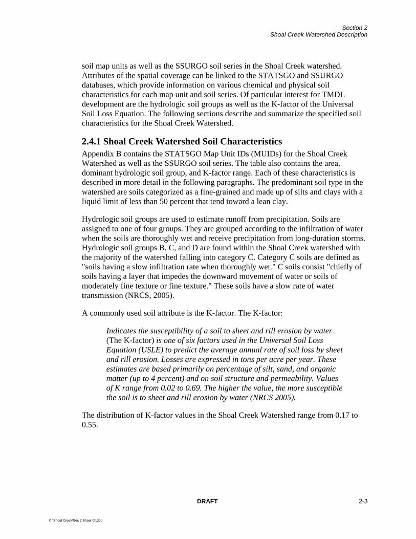
2.4.1 Shoal Creek Watershed Soil Characteristics Appendix B contains the STATSGO Map Unit IDs (MUIDs) for the Shoal Creek Watershed as well as the SSURGO soil series. The table also contains the area, dominant hydrologic soil group, and K-factor range. Each of these characteristics is described in more detail in the following paragraphs. The predominant soil type in the watershed are soils categorized as a fine-grained and made up of silts and clays with a liquid limit of less than 50 percent that tend toward a lean clay.
Hydrologic soil groups are used to estimate runoff from precipitation. Soils are assigned to one of four groups. They are grouped according to the infiltration of water when the soils are thoroughly wet and receive precipitation from long-duration storms. Hydrologic soil groups B, C, and D are found within the Shoal Creek watershed with the majority of the watershed falling into category C. Category C soils are defined as "soils having a slow infiltration rate when thoroughly wet." C soils consist "chiefly of soils having a layer that impedes the downward movement of water or soils of moderately fine texture or fine texture." These soils have a slow rate of water transmission (NRCS, 2005).
A commonly used soil attribute is the K-factor. The K-factor:
Indicates the susceptibility of a soil to sheet and rill erosion by water. (The K-factor) is one of six factors used in the Universal Soil Loss Equation (USLE) to predict the average annual rate of soil loss by sheet and rill erosion. Losses are expressed in tons per acre per year. These estimates are based primarily on percentage of silt, sand, and organic matter (up to 4 percent) and on soil structure and permeability. Values of K range from 0.02 to 0.69. The higher the value, the more susceptible the soil is to sheet and rill erosion by water (NRCS 2005).
The distribution of K-factor values in the Shoal Creek Watershed range from 0.17 to 0.55.
DRAFT 2-3
C:\Shoal Creek\Sec 2 Shoal Cr.doc

Section 2 Shoal Creek Watershed Description
2.5 Population Population data were retrieved from Census 2000 TIGER/Line Data from the U.S. Bureau of the Census. Geographic shape files of census blocks were downloaded for every county containing any portion of the watersheds. The block files were clipped to each watershed so that only block populations associated with the watershed would be counted. The census block demographic text file (PL94) containing population data was downloaded and linked to each watershed and summed. City populations were taken from the US Bureau of the Census. For municipalities that are located across watershed borders, the population was estimated based on the percentage of area of municipality within the watershed boundary. Approximately 15,837 people reside in the watershed. The major municipalities in the Shoal Creek watershed are shown in Figure 1-1. The city of Breese is the largest population center in the watershed and contributes an estimated 4,048 people to total watershed population.
2.6 Climate and Streamflow 2.6.1 Climate Southern Illinois has a temperate climate with hot summers and cold, snowy winters. Monthly precipitation and temperature data from Hillsboro (station id. 4108) in Montgomery County were extracted from the NCDC database for the years of 1901 through 2004. The data station in Hillsboro, Illinois is just north of the watershed and was chosen to be representative of precipitation throughout the Shoal Creek watershed which is lacking an active weather station within its boundary.
Table 2-2 contains the average monthly precipitation along with average high and low temperatures for the period of record. The average annual precipitation is approximately 39 inches.
Table 2-2 Average Monthly Climate Data in the Shoal Creek Watershed
Month Total Precipitation
(inches) Maximum Temperature
(degrees F) Minimum Temperature
(degrees F) January 2.3 38 21 February 2 43 24 March 3.3 54 33 April 4 66 43 May 4.5 76 53 June 4.2 85 62 July 3.4 89 66 August 3.5 88 64 September 3.4 81 56 October 3.1 70 45 November 3 54 34 December 2.5 42 25
Total 39.2
2-4 DRAFT
C:\Shoal Creek\Sec 2 Shoal Cr.doc

Section 2 Shoal Creek Watershed Description
2.6.2 Streamflow Analysis of the Shoal Creek Watershed requires an understanding of flow throughout the drainage area. USGS gage 05594000 (Shoal Creek near Breese, Illinois) is the only available data gage within the watershed with current data (Figure 2-4). The gage is located on the OI 08 segment of Shoal Creek.
Data was available for the gage from the USGS for the years 1909 through 2004. The average monthly flows recorded at the gage range from 138 cubic feet per second (cfs) in September to 978 cfs in March with a mean annual monthly flow of 548 cfs (Figure 2-5).
DRAFT 2-5
C:\Shoal Creek\Sec 2 Shoal Cr.doc

Section 2 Shoal Creek Watershed Description
THIS PAGE INTENTIONALLY LEFT BLANK
2-6 DRAFT
C:\Shoal Creek\Sec 2 Shoal Cr.doc

Figure 2-1Shoal Creek Watershed
Elevation
DRAFT
Lake Fork
Breese
Pocahontas
Bearc
atC
reek
New Douglas
Dry
Fork
Dorris Cre
ek
India
nCre
ek
LittleD
ryFork
Shoal C
reek
OI 09
SorentoROZH
Locust Fork
OIC
02
Cattle CreekOIP 10
Chicken Creek
OIO09
Sh
oalC
reek
OI08
ShoalC
reek
OI05
§̈¦I-70
£¤127
£¤140
£¤143
£¤50
£¤161
Mac
ou
pin
Cn
ty
Clinton CntyBond Cnty
Mo
ntg
om
ery
Cn
ty
Mad
iso
nC
nty B
on
dC
nty
0 5 102.5 Miles
/
Elevation (feet)
394 - 405
406 - 420
421 - 435
436 - 450
451 - 465
466 - 480
481 - 495
496 - 510
511 - 525
526 - 540
541 - 555
556 - 570
571 - 585
586 - 600
601 - 615
616 - 630
631 - 645
646 - 660
661 - 675
676 - 690
691 - 699
Lake or Reservoir
Legend
Interstate
US and State Highway
Railroad
County Boundary
303(d) Listed Waterbody
Watershed
Major Stream

Section 2 Shoal Creek Watershed Description
THIS PAGE INTENTIONALLY LEFT BLANK
2-8 DRAFT
C:\Shoal Creek\Sec 2 Shoal Cr.doc
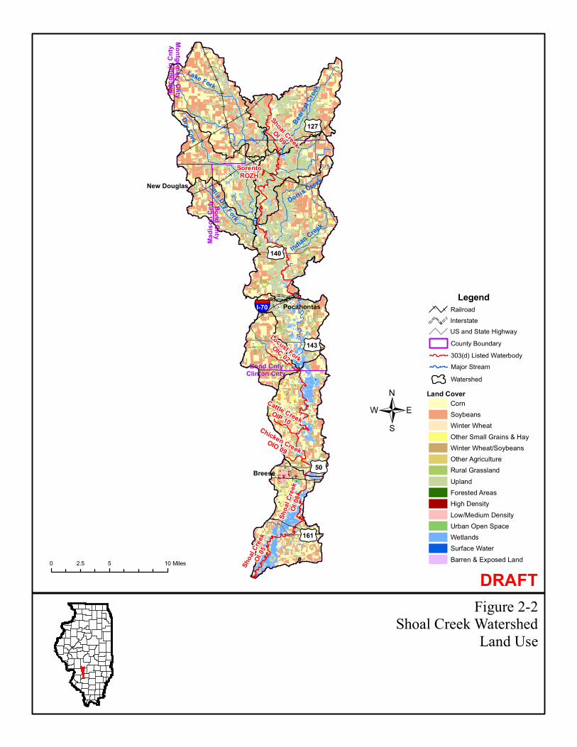
Figure 2-2Shoal Creek Watershed
Land Use
DRAFT
Lake Fork
Breese
Pocahontas
Bearc
atC
reek
New Douglas
Dry
Fork
Dorris Cre
ek
India
nCre
ek
LittleD
ryFork
Shoal C
reek
OI 09
SorentoROZH
Locust Fork
OIC
02
Cattle CreekOIP 10
Chicken Creek
OIO09
Sh
oalC
reek
OI08
ShoalC
reek
OI05
§̈¦I-70
£¤127
£¤140
£¤143
£¤50
£¤161
Mac
ou
pin
Cn
ty
Clinton CntyBond Cnty
Mo
ntg
om
ery
Cn
ty
Mad
iso
nC
nty B
on
dC
nty
0 5 102.5 Miles
/
Legend
Land Cover
Corn
Soybeans
Winter Wheat
Other Small Grains & Hay
Winter Wheat/Soybeans
Other Agriculture
Rural Grassland
Upland
Forested Areas
High Density
Low/Medium Density
Urban Open Space
Wetlands
Surface Water
Barren & Exposed Land
Interstate
US and State Highway
Railroad
County Boundary
303(d) Listed Waterbody
Watershed
Major Stream

Section 2 Shoal Creek Watershed Description
THIS PAGE INTENTIONALLY LEFT BLANK
2-10 DRAFT
C:\Shoal Creek\Sec 2 Shoal Cr.doc

Figure 2-3Shoal Creek Watershed
Soils
DRAFT
Lake Fork
Breese
Pocahontas
Bearc
atC
reek
New Douglas
Dry
Fork
Dorris Cre
ek
India
nCre
ek
LittleD
ryFork
Shoal C
reek
OI 09
SorentoROZH
Locust Fork
OIC
02
Cattle CreekOIP 10
Chicken Creek
OIO09
Sh
oalC
reek
OI08
ShoalC
reek
OI05
§̈¦I-70
£¤127
£¤140
£¤143
£¤50
£¤161
Mac
ou
pin
Cn
ty
Clinton CntyBond Cnty
Mo
ntg
om
ery
Cn
ty
Mad
iso
nC
nty B
on
dC
nty
0 5 102.5 Miles
/
IL004
IL005
IL006
IL029
IL037
IL051
IL068
8F
31A
46A
50A
113A
113B
119C3
127B
438C2
438B
474A
491C2
517A
517B
581B2
582B
657A
703A
878C3
880B2
882B
885A
894A
914C3
993A
3333A
3451A
8D3
119D2
119D3
914D3
STATSGO/SSURGO Soil Units
Lake or Reservoir
Legend
Interstate
US and State Highway
Railroad
County Boundary
303(d) Listed Waterbody
Watershed
Major Stream

Section 2 Shoal Creek Watershed Description
THIS PAGE INTENTIONALLY LEFT BLANK
2-12 DRAFT
C:\Shoal Creek\Sec 2 Shoal Cr.doc

Figure 2-4Shoal Creek Watershed
USGS Gage
DRAFT
#*#*#*
Lake Fork
Breese
PocahontasB
earc
atC
reek
New Douglas
Dry
Fork
Dorris Cre
ek
India
nCre
ek
LittleD
ryFork
Shoal C
reek
OI 09
SorentoROZH
Locust Fork
OIC
02
Cattle CreekOIP 10
Chicken Creek
OIO09
Sh
oalC
reek
OI08
ShoalC
reek
OI05
§̈¦I-70
£¤127
£¤140
£¤143
£¤50
£¤161
Mac
ou
pin
Cn
ty
Clinton CntyBond Cnty
Mo
ntg
om
ery
Cn
ty
Mad
iso
nC
nty B
on
dC
nty
Germantown
Pierron
Sorento
Shoal Creeknear Breese, IL
0 5 102.5 Miles
/
Legend
Interstate
US and State Highway
Railroad
County Boundary
Watershed
Municipality
Lake or Reservoir
Major Stream
303(d) Listed Waterbodies
#* USGS Gage
Section 2 Shoal Creek Watershed Description
THIS PAGE INTENTIONALLY LEFT BLANK
2-14 DRAFT
C:\Shoal Creek\Sec 2 Shoal Cr.doc

A
T:\GIS\WRITEUP\8 Shoal Creek\Data\Shoal_precip-temp-flow.xlsflowchart
Figure 2-5:Average Total Monthly Streamflow
at USGS gage 05594000Shoal Creek near Breese, IL
0
200
400
600
800
1000
1200
Jan Feb Mar Apr May Jun Jul Aug Sep Oct Nov Dec
Month
cfs
Average Monthly Total Streamflow

Section 2 Shoal Creek Watershed Description
THIS PAGE INTENTIONALLY LEFT BLANK
2-16 DRAFT
T:\GIS\IEPA STAGE ONE TMDL DRAFTS\WP\8 Shoal Creek\Sec 2 Shoal Cr.doc

Section 3 Public Participation and Involvement 3.1 Shoal Creek Watershed Public Participation and Involvement Public knowledge, acceptance, and follow through are necessary to implement a plan to meet recommended TMDLs. It is important to involve the public as early in the process as possible to achieve maximum cooperation and counter concerns as to the purpose of the process and the regulatory authority to implement any recommendations.
Illinois EPA, along with CDM, will hold up to four public meetings within the watershed throughout the course of the TMDL development. This section will be updated once public meetings have occurred.
DRAFT 3-1
C:\Shoal Creek\Sec 3 Shoal Cr.doc

Section 3 Public Participation and Involvement
THIS PAGE INTENTIONALLY LEFT BLANK
3-2 FINAL
C:\Shoal Creek\Sec 3 Shoal Cr.doc
Section 4 Shoal Creek Watershed Water Quality Standards 4.1 Illinois Water Quality Standards Water quality standards are developed and enforced by the state to protect the "designated uses" of the state's waterways. In the state of Illinois, setting the water quality standards is the responsibility of the Illinois Pollution Control Board (IPCB). Illinois is required to update water quality standards every three years in accordance with the CWA. The standards requiring modifications are identified and prioritized by Illinois EPA, in conjunction with USEPA. New standards are then developed or revised during the three-year period.
Illinois EPA is also responsible for developing scientifically based water quality criteria and proposing them to the IPCB for adoption into state rules and regulations. The Illinois water quality standards are established in the Illinois Administrative Rules Title 35, Environmental Protection; Subtitle C, Water Pollution; Chapter I, Pollution Control Board; Part 302, Water Quality Standards.
4.2 Designated Uses The waters of Illinois are classified by designated uses, which include: General Use, Public and Food Processing Water Supplies, Lake Michigan, and Secondary Contact and Indigenous Aquatic Life Use (Illinois EPA 2005). The designated uses applicable to the Shoal Creek Watershed are the General Use and Public and Food Processing Water Supplies Use.
4.2.1 General Use The General Use classification is defined by IPCB as: The General Use standards will protect the state's water for aquatic life, wildlife, agricultural use, secondary contact use and most industrial uses and ensure the aesthetic quality of the state's aquatic environment. Primary contact uses are protected for all General Use waters whose physical configuration permits such use.
4.2.2 Public and Food Processing Water Supplies The Public and Food Processing Water Supplies Use is defined by IPCB as: These are cumulative with the general use standards of Subpart B and must be met in all waters designated in Part 303 at any point at which water is withdrawn for treatment and distribution as a potable supply or for food processing.
4.3 Illinois Water Quality Standards To make 303(d) listing determinations for aquatic life uses, Illinois EPA first collects biological data and if this data suggests that impairment to aquatic life is occurring, then a comparison of available water quality data with water quality standards occurs.
DRAFT 4-1
C:\Shoal Creek\Sec 4 Shoal Cr.doc

Section 4 Shoal Creek Watershed Water Quality Standards
For public and food processing water supply waters, Illinois EPA compares available data with water quality standards to make impairment determinations. Tables 4-1 and 4-2 present the water quality standards of the potential causes of impairment for both lakes and streams within the Shoal Creek Watershed. Only constituents with numeric water quality standards will have TMDLs developed at this time.
Table 4-1 Summary of Water Quality Standards for Potential Shoal Creek Watershed Lake Impairments
Parameter Units General Use Water Quality Standard
Public and Food Processing Water Supplies
Excess Algal Growth
NA No numeric standard No numeric standard
Manganese µg/L 1000 150
Total Phosphorus mg/L 0.05(1) No numeric standard
Total Suspended Solids
NA No numeric standard No numeric standard
(1) Standard applies in particular inland lakes and reservoirs (greater than 20 acres) and in any stream at the point where it enters any such lake or reservoir. Sorento Reservoir is less than 20 acres. µg/L = micrograms per liter mg/L = milligrams per liter NA = Not Applicable
Table 4-2 Summary of Water Quality Standards for Potential Shoal Creek Watershed Stream Impairments
Parameter Units General Use Water Quality Standard
Public and Food Processing Water Supplies
Acute standard(1) = (exp[-1.464+0.9422 x
ln(H)]) x 0.960* Chronic standard(2) =
Copper µg/L
(exp[-1.465+0.8545 x ln(H)]) x 0.960*
No numeric standard
Manganese µg/L 1000 150
Nitrogen, ammonia (Total)
mg/L 15(3) No numeric standard
5.0 instantaneous minimum;
Oxygen, Dissolved mg/L
6.0 minimum during at least 16 hours of any 24
hour period
No numeric standard
Sedimentation/ Siltation
NA No numeric standard No numeric standard
Silver µg/L 5 No numeric standard
Total Dissolved Solids
µg/L 1000 500
4-2 DRAFT
C:\Shoal Creek\Sec 4 Shoal Cr.doc

Section 4 Shoal Creek Watershed Water Quality Standards
Table 4-2 Summary of Water Quality Standards for Potential Shoal Creek Watershed Stream Impairments (continued)
Parameter Units General Use Water Quality Standard
Public and Food Processing Water Supplies
May through Oct – 200(4), 400(5)
Total Fecal Coliform Count/ 100 mL
Nov though Apr – no numeric standard
2000(4)
Total Nitrogen as N NA No numeric standard No numeric standard
Total Phosphorus - Statistical Guideline
NA No numeric standard No numeric standard
Total Suspended Solids
NA No numeric standard No numeric standard
µg/L = micrograms per liter exp(x) = base natural logarithms raised to the x- power mg/L = milligrams per liter ln(H) = natural logarithm of hardness of the receiving water in mg/L NA = Not Applicable * = conversion factor for multiplier for dissolved metals (1) Not to be exceeded except as provided in 35 Ill. Adm. Code 302.208(d). (2) Not to be exceeded by the average of at least four consecutive samples collected over any period of at least four days except as provided in 35 Ill. Adm. Code 302.208(d). The samples used to demonstrate attainment or lack of attainment with a chronic standard must be collected in a manner that assures an average representative of the sampling period. To calculate attainment status of chronic metals standards, the concentration of the metal in each sample is divided by the calculated water quality standard for the sample to determine a quotient. The water quality standard is attained if the mean of the sample quotients is less than or equal to one for the duration of the averaging period. (3) The allowable concentration varies in accordance with water temperature and pH values. 15 mg/L is the maximum total ammonia nitrogen value allowed. In general, as both temperature and pH decrease, the allowable value of total ammonia nitrogen increases. For example, when the pH is 8.0 and the temperature is 20 degrees C, the acute standard is 8.4 mg/L, the chronic standard is 1.7 mg/L, and the subchronic standard is 4.3 mg/L. See 35 Ill. Adm. Code 302.212 for the formulae by which the standards are calculated. (4) Geometric mean based on a minimum of 5 samples taken over not more than a 30 day period. (5) Standard shall not be exceeded by more than 10% of the samples collected during any 30 day period.
4.4 Potential Pollutant Sources In order to properly address the conditions within the Shoal Creek watershed, potential pollution sources must be investigated for the pollutants where TMDLs will be developed. The following is a summary of the potential sources associated with the listed causes for the 303(d) listed segments in this watershed. They are summarized in Table 4-3.
DRAFT 4-3
C:\Shoal Creek\Sec 4 Shoal Cr.doc

Section 4 Shoal Creek Watershed Water Quality Standards
Table 4-3 Summary of Potential Sources for Shoal Creek Watershed Segment ID Segment Name Potential Causes Potential Sources OI 05 Shoal Creek Sedimentation/siltation,
dissolved oxygen, total suspended solids, total phosphorus
Agriculture, crop-related sources, nonirrigated crop production, intensive animal feeding operations
OI 08 Shoal Creek Manganese, total fecal coliform Source unknown OIC 02 Locust Fork Manganese,
sedimentation/siltation, dissolved oxygen, total suspended solids, total phosphorus
Agriculture, crop-related sources, nonirrigated crop production, intensive animal feeding operations, source unknown
OIO 09 Chicken Creek Silver, total nitrogen as N, sedimentation/siltation, dissolved oxygen, total suspended solids, total phosphorus
Agriculture, crop-related sources, nonirrigated crop production, pasture grazing – riparian and/or upland, intensive animal feeding operations, source unknown
OIP 10 Cattle Creek Copper, ammonia nitrogen (total), sedimentation/siltation, dissolved oxygen, total dissolved solids, total suspended solids, total phosphorus
Agriculture, crop-related sources, nonirrigated crop production, pasture grazing – riparian and/or upland, intensive animal feeding operations, source unknown
OI 09 Shoal Creek Manganese, total fecal coliform Source unknown ROZH Sorento
Reservoir Manganese, total suspended solids, excess algal growth, total phosphorus
Agriculture, crop-related sources, nonirrigated crop production, source unknown
4-4 DRAFT
C:\Shoal Creek\Sec 4 Shoal Cr.doc
Section 5 Shoal Creek Watershed Characterization Data was collected and reviewed from many sources in order to further characterize the Shoal Creek watershed. Data has been collected in regards to water quality, reservoirs, and both point and nonpoint sources. This information is presented and discussed in further detail in the remainder of this section.
5.1 Water Quality Data There are nine historic water quality stations within the Shoal Creek watershed that were used for this report. Figure 5-1 shows the water quality data stations within the watershed that contain data relevant to the impaired segments.
The impaired water body segments in the Shoal Creek watershed were presented in Section 1. Refer to Table 1-1 for impairment information specific to each segment. The following sections address both stream and lake impairments. Data is summarized by impairment and discussed in relation to the relevant Illinois numeric water quality standard. Data analysis is focused on all available data collected since 1990. STORET data is available for stations sampled prior to January 1, 1999 while Illinois EPA data (electronic and hard copy) are available for stations sampled after that date. The following sections will first discuss Shoal Creek watershed stream data followed by Shoal Creek watershed reservoir data.
5.1.1 Stream Water Quality Data The Shoal Creek watershed has six impaired stream segments within its drainage area that are addressed in this report. There is one active water quality station on each impaired segment (see Figure 5-1). The data summarized in this section include water quality data for impaired constituents as well as parameters that could be useful in future modeling and analysis efforts. All historic data is available in Appendix C.
5.1.1.1 Fecal Coliform Shoal Creek segments OI 08 and OI 09 are listed as impaired for total fecal coliform. Table 5-1 summarizes available historic fecal coliform data on the segment. The general use water quality standard for fecal coliform states that the standard of 200 per 100 mL not be exceeded by the geometric mean of at least five samples, nor can 10 percent of the samples collected exceed 400 per 100 mL in protected waters, except as provided in 35 Ill. Adm. Code 302.209(b). Samples must be collected over a 30 day period or less during peak fecal coliform application periods (May through October).The public water supply water quality standard states that the standard of 2,000 per 100 mL not be exceeded by the geometric mean of at least five samples.
DRAFT 5-1
C:\Shoal Creek\Sec 5 Shoal Cr.doc

Section 5 Shoal Creek Watershed Characterization
Table 5-1 Existing Fecal Coliform Data for Shoal Creek Watershed Impaired Stream Segments
Sample Location and Parameter
Period of Record and Number of
Data Points
Geometric mean of all
samples Maximum Minimum
Number of
samples > 200 (1)
Number of
samples > 400 (1)
Number of
samples > 2000
Shoal Creek Segment OI 08; Sample Location OI 08 Total Fecal Coliform (cfu/100 mL)
2000-2005; 39 401 22,000 2 13 10 4
Shoal Creek Segment OI 09; Sample Location OI 09 Total Fecal Coliform (cfu/100 mL)
2000-2002; 18 449 38,600 10 6 4 1
(1) Samples collected during the months of May through October There are no instances since 1990 where at least five samples have been collected during a 30-day period. The summary of data presented in Table 5-1 reflects single samples compared to the standards during the appropriate months. Figure 5-2 shows the total fecal coliform samples collected over time at OI 08 and OI 09.
5.1.1.2 Dissolved Oxygen In the Shoal Creek watershed, Shoal Creek segment OI 05, Locust Fork segment OIC 02, Chicken Creek segment OIO 09, and Cattle Creek segment OIP 10 are listed as impaired for dissolved oxygen (DO). Table 5-2 summarizes the available historic DO data since 1990 for the impaired stream segments (raw data contained in Appendix C). The table also shows the number of violations for each segment. A sample was considered a violation if it was below 5.0 mg/L. The average DO concentration is below the standard (5.0 mg/L instantaneous minimum) on two of the four impaired segments. Minimum values for all segments are below the DO standard.
Table 5-2 Existing Dissolved Oxygen Data for Shoal Creek Watershed Impaired Stream Segments
Sample Location and Parameter
Illinois WQ Standard
(mg/L)
Period of Record and Number of Data Points Mean Maximum Minimum
Number of Violations
Shoal Creek Segment OI 05; Sample Location OI 05 DO 5.0(1) 2002; 3 5.4 6.5 4.0 1 Locust Fork Segment OIC 02; Sample Locations OIC 02 DO 5.0(1) 1991; 3 4.4 9.3 1.7 1 Chicken Creek Segment OIO 09; Sample Location OIO 09 DO 5.0(1) 1991; 2 5.0 6.7 3.3 1 Cattle Creek Segment OIP 10; Sample Location OIP 10 DO 5.0(1) 1991; 3 4.2 8.4 0.1 2 (1) Instantaneous Minimum Table 5-3 contains information on data availability for other parameters that may be useful in data needs analysis and future modeling efforts for DO. Where available, all nutrient, biological oxygen demand (BOD), and total organic carbon data has been collected for possible use in future analysis.
5-2 DRAFT
C:\Shoal Creek\Sec 5 Shoal Cr.doc

Section 5 Shoal Creek Watershed Characterization
Table 5-3 Data Availability for DO Data Needs Analysis and Future Modeling Efforts
Sample Location and Parameter Available Period of Record Post 1990
Number of Samples
Shoal Creek Segment OI 05; Sample Location OI 05 Nitrogen Kjeldahl Total Bottom Dep Dry Wt (mg/kg) 1996 1 Phosphorus, Total, Bottom Deposit (mg/kg-P Dry Wgt) 1996 1 Locust Fork Segment OIC 02; Sample Locations OIC 02 Ammonia, Unionized (Calc Fr Temp-pH-NH4) (mg/L) 1991 3 Ammonia, Unionized (mg/L as N) 1991 3 BOD, 5 Day, 20 Deg C (mg/L) 1991 3 BOD, Carbonaceous, 5 Day, 20 Deg C (mg/L) 1991 3 COD, .025N K2CR2O7 (mg/L) 1991 3 COD, Bottom Deposits, Dry Weight (mg/kg) 1991 1 Nitrite plus Nitrate, Total 1 Det. (mg/L as N) 1991 3 Nitrogen Kjeldahl Total Bottom Dep Dry Wt (mg/kg) 1991 1 Nitrogen, Ammonia, Total (mg/L as N) 1991 3 Nitrogen, Kjeldahl, Total (mg/L as N) 1991 3 Phosphorus, Total (mg/L as P) 1991 3 Phosphorus, Total, Bottom Deposit (mg/kg-P Dry Wgt) 1991 1 Chicken Creek Segment OIO 09; Sample Location OIO 09 Ammonia, Unionized (Calc Fr Temp-pH-NH4) (mg/L) 1991 2 Ammonia, Unionized (mg/L as N) 1991 2 BOD, 5 Day, 20 Deg C (mg/L) 1991 2 BOD, Carbonaceous, 5 Day, 20 Deg C (mg/L) 1991 2 COD, .025N K2CR2O7 (mg/L) 1991 2 Nitrite plus Nitrate, Total 1 Det. (mg/L as N) 1991 2 Nitrogen, Ammonia, Total (mg/L as N) 1991 2 Nitrogen, Kjeldahl, Total (mg/L as N) 1991 2 Phosphorus, Total (mg/L as P) 1991 2 Cattle Creek Segment OIP 10; Sample Location OIP 10 Ammonia, Unionized (Calc Fr Temp-pH-NH4) (mg/L) 1991 3 Ammonia, Unionized (mg/L as N) 1991 3 BOD, 5 Day, 20 Deg C (mg/L) 1991 3 BOD, Carbonaceous, 5 Day, 20 Deg C (mg/L) 1991 3 COD, .025N K2CR2O7 (mg/L) 1991 3 Nitrite plus Nitrate, Total 1 Det. (mg/L as N) 1991 3 Nitrogen, Ammonia, Total (mg/L as N) 1991 3 Nitrogen, Kjeldahl, Total (mg/L as N) 1991 3 Phosphorus, Total (mg/L as P) 1991 3 5.1.1.3 Total Ammonia Segment OIP10 of Cattle Creek is listed as impaired for total ammonia nitrogen. The allowable concentration of total ammonia varies as it is calculated using water temperature and pH values. Regardless of temperature and pH variation, the State sets 15 mg/L as the maximum total ammonia nitrogen value allowed. There have been three samples collected on the segment since 1990. Table 5-4 contains the sampling results. The sample collected in September of 1991 exceeded the maximum allowable concentration.
Table 5-4 Total Ammonia Samples Collected on Cattle Creek segment OIP10
Sample Location Sample Date
Total Ammonia
(mg/L) OIP 10 4/15/91 0.38 OIP 10 9/18/91 24 OIP 10 10/28/91 3.0
DRAFT 5-3
C:\Shoal Creek\Sec 5 Shoal Cr.doc

Section 5 Shoal Creek Watershed Characterization
5.1.1.4 Metals: Silver and Copper Chicken Creek segment OIO 09 is impaired for silver and Cattle Creek segment OIP 10 is impaired for copper. Table 5-5 contains a summary of metal data collected on impaired segments. The applicable water quality standard for silver is a maximum total silver concentration of 5.0 µg/L. The applicable copper water quality standard is dependent on water hardness. Hardness data has been collected in conjunction with copper data. The number of violations presented in Table 5-5 for copper represents violations of the general use chronic standard. There were not enough available total silver or dissolved copper data for time series plots. Table 5-5 shows that one of the two total silver samples and two of three dissolved copper samples violated the corresponding water quality standards.
Table 5-5 Existing Metals Data (Silver and Copper) for Shoal Creek Watershed Impaired Stream Segments
Sample Location and Parameter
Illinois WQ Standard
(µg/L)
Period of Record and Number of Data Points Mean Maximum Minimum
Number of Violations
Chicken Creek Segment OIO 09; Sample Location OIO 09 Total Silver (µg/L) General Use:
5.0 1991; 2 8 13 3 1
Cattle Creek Segment OIP 10; Sample Location OIP 10 Dissolved Copper (µg/L)
Hardness Dependent
1991; 3 502 1,461 10 2
5.1.1.5 Other Constituents: Manganese and Total Dissolved Solids Shoal Creek segments OI 08 and OI 09 and Locust Fork segment OIC 02 are impaired for manganese. The applicable water quality standard is a maximum total manganese concentration of 1,000 µg/L for general use and 150 µg/L for public water supply. Cattle Creek segment OIP 10 is impaired for total dissolved solids (TDS). The applicable water quality standard for TDS is a maximum TDS concentration of 1,000 mg/L for general use and 500 mg/L for public water supply. Standards for the general use waters cannot be exceeded except where mixing is allowed as provided in 35 Ill. Adm. Code 302.102.
Table 5-6 summarizes the available historic manganese and TDS data since 1990 for the impaired stream segments. This includes dissolved and bottom deposit manganese samples where available. The table also shows the number of violations for each segment. Figure 5-3 shows total manganese concentrations over time on Shoal Creek segments OI 08 and OI 09. There is limited manganese and TDS data for segments OIC 02 and OIP 10. These impaired segments have only three data points each.
5-4 DRAFT
C:\Shoal Creek\Sec 5 Shoal Cr.doc

Section 5 Shoal Creek Watershed Characterization
Table 5-6 Existing Chemical Constituents Data (Manganese and Total Dissolved Solids) for Shoal Creek Watershed Impaired Stream Segments
Sample Location and Parameter
Illinois WQ Standard
|(µg/L or mg/L)
Period of Record and Number of Data Points Mean Maximum Minimum
Number of Violations
Shoal Creek Segment OI 08; Sample Location OI 08 General Use:
1000 0 Total Manganese
(µg/L) Public Water Supply: 150
1990-2003; 41 269 680 76
35
Dissolved Manganese (µg/L)
NA 1990-2003; 41 131 570 15 NA
Shoal Creek Segment OI 09; Sample Location OI 09 General Use:
1000 0 Total Manganese
(µg/L) Public Water Supply: 150
1990-2002; 26 214 370 71
18
Locust Fork Segment OIC 02; Sample Locations OIC 02 General Use:
1000 1 Total Manganese
(µg/L) Public Water Supply: 150
1991; 3 1,557 4,202 164
3
Manganese Sediments (mg/kg)
NA 1991; 1 624 624 624 NA
Cattle Creek Segment OIP 10; Sample Location OIP 10 General Use:
1000 1 TDS (µg/L)
Public Water Supply: 150
1991; 3 719 1,220 304
2
5.1.2 Reservoir Water Quality Data The Shoal Creek watershed has one impaired reservoir within its drainage area that is addressed in this report. There are three monitoring stations on the impaired reservoir (see Figure 5-1). The data summarized in this section include water quality data for the impaired constituent as well as parameters that could be useful in future modeling and analysis efforts. All historic data is available in Appendix C.
5.1.2.1 Sorento Reservoir Sorento Reservoir is impaired for total manganese. Although there are three monitoring stations in Sorento Reservoir, manganese data is only available from sampling location ROZH-1. An inventory of all available manganese data is presented in Table 5-7.
Table 5-7 Sorento Reservoir Data Inventory for Impairments Sorento Reservoir Segment ROZH; Sample Locations ROZH-1 ROZH-1 Period of Record Number of Samples Total Manganese 2001 5 Manganese Bottom Deposits 2001 1
The applicable water quality standard for manganese is a maximum concentration of 1,000 µg/L for general use and 150 µg/L for public water supplies. Table 5-8 summarizes available manganese data for Sorento Reservoir. Three of the five samples taken in 2001 violated the public water supply standard.
DRAFT 5-5
C:\Shoal Creek\Sec 5 Shoal Cr.doc

Section 5 Shoal Creek Watershed Characterization
Table 5-8 Average Total Manganese Concentrations in Sorento Reservoir ROZH-1
Year Water Quality Standard (mg/L) Data Count Number of Violations Average
General Use: 1000 0 2001 Public Water Supply: 150 5 3 269
Table 5-9 contains information on data availability for other parameters that may be useful in data needs analysis and future modeling efforts. DO at varying depths has been collected where available.
Table 5-9 Sorento Reservoir Data Availability for Data Needs Analysis and Future Modeling Efforts Sorento Reservoir Segment ROZH; Sample Locations ROZH-1, ROZH-2, and ROZH-3 ROZH-1 Period of Record Number of Samples Total Depth 1996-1998 17 Dissolved Oxygen 2001 44 Temperature 2001 44 ROZH-2 Total Depth 1990-1998 16 ROZH-3 Total Depth 1990-1998 17 5.2 Reservoir Characteristics There is one impaired reservoir in the Shoal Creek watershed. Reservoir information that can be used for future modeling efforts was collected from GIS analysis, Illinois EPA, the U.S. Army Corps of Engineers, and USEPA water quality data. The following sections will discuss the available data for Sorento Reservoir.
5.2.1 Sorento Reservoir Sorento Reservoir has a surface area of 11 acres. Water from the lake is supplied to the Village of Sorento for drinking water from an intake in Sorento Reservoir and Shoal Creek at a rate of approximately 70,000 gallons per day (Source Water Assessment Program, Illinois EPA 2002). Table 5-10 contains dam information for the reservoir while table 5-11 contains depth information for each sampling location on the reservoir. The average maximum depth in Sorento Reservoir is 21.1 feet.
Table 5-10 Sorento Reservoir Dam Information (U.S. Army Corps of Engineers) Dam Length 270 feet Dam Height 27 feet Maximum Discharge 1,025 cfs Maximum Storage 162 acre-feet Normal Storage 101 acre-feet Spillway Width 53 feet Outlet Gate Type U
5-6 DRAFT
C:\Shoal Creek\Sec 5 Shoal Cr.doc

Section 5 Shoal Creek Watershed Characterization
Table 5-11 Average Depths (ft) for Sorento Reservoir (Illinois EPA 2002 and USEPA 2002a) Year ROZH-1 ROZH-2 ROZH-3 1996 17.2 10.0 4.6 1997 23.1 9.6 7.2 1998 27.5 11.2 4.0 2001 16.5 – –
Average 21.1 10.3 5.3 5.3 Point Sources Point sources for the Shoal Creek watershed have been separated into municipal/ industrial sources and mining discharges. Available data has been summarized and are presented in the following sections.
5.3.1 Municipal and Industrial Point Sources Permitted facilities must provide Discharge Monitoring Reports (DMRs) to Illinois EPA as part of their NPDES permit compliance. DMRs contain effluent discharge sampling results, which are then maintained in a database by the state. There are 10 point sources located within the Shoal Creek watershed. Figure 5-4 shows all NPDES permitted facilities in the watershed. In order to assess point source contributions to the watershed, the data has been examined by receiving water and then by the downstream impaired segment that has the potential to receive the discharge. Receiving waters were determined through information contained in the USEPA Permit Compliance System (PCS) database. Maps were used to determine downstream impaired receiving water information when PCS data was not available. The impairments for each segment or downstream segment were considered when reviewing DMR data. Data has been summarized for any sampled parameter that is associated with a downstream impairment (i.e., all available nutrient and biological oxygen demand data was reviewed for segments that are impaired for dissolved oxygen). This will help in future model selection as well as source assessment and load allocation.
5.3.1.1 Shoal Creek Segment OI 05 There are two point sources with the potential to contribute discharge to Shoal Creek segment OI 05. Segment OI 05 is listed as impaired for DO. Table 5-12 contains a summary of available and pertinent DMR data for these point sources.
Table 5-12 Effluent Data from Point Sources Discharging Upstream of Shoal Creek Segment OI 05 (Illinois EPA 2005) Facility Name Period of Record Permit Number
Receiving Water/ Downstream Impaired Waterbody Constituent
Average Value
Average Loading
(lb/d) Average Daily Flow 0.0187 mgd NA BOD, 5-Day 191.3 mg/L
Western Gardens MHP 1996-2004 ILG551030
NA/Shoal Creek Segment OI 05
CBOD, 5-Day 87.9 mg/L 4.31
Average Daily Flow 0.135 mgd NA BOD, 5-Day 49.0 mg/L
Germantown STP 1998-2005 ILG580186
Shoal Creek/Shoal Creek Segment OI05
CBOD, 5-Day 14.0 mg/L 15.1
DRAFT 5-7
C:\Shoal Creek\Sec 5 Shoal Cr.doc

Section 5 Shoal Creek Watershed Characterization
5.3.1.2 Shoal Creek Segment OI 08 There are four permitted facilities whose discharge has the potential to reach Shoal Creek segment OI 08. Shoal Creek segment OI 08 is listed for manganese and total fecal coliform impairments. Table 5-13 contains a summary of available DMR data for these point sources. Total fecal coliform data was available for only one discharger.
Table 5-13 Effluent Data from Point Sources Discharging to Shoal Creek Segment OI 08 (Illinois EPA 2005) Facility Name Period of Record Permit Number
Receiving Water/ Downstream Impaired Waterbody Constituent
Average Value
Average Loading
(lb/d) Pierron East STP 2001-2005 ILG580237
Unnamed Tributary to Shoal Creek/Shoal Creek Segment OI 08
Average Daily Flow 0.0206 mgd NA
Average Daily Flow 0.629 mgd NA Breese STP 1989-2004 IL0022772
Unnamed Tributary to Shoal Creek/Shoal Creek Segment OI 08
Total Fecal Coliform 44.4 mg/L
Louisville STP 1994-2004 ILG580081
NA/Shoal Creek Segment OI 08
Average Daily Flow 0.15 mgd NA
Pocahontas STP 1993-2005 ILG580010
Shoal Creek/Shoal Creek Segment OI 08
Average Daily Flow 0.125 mgd NA
5.3.1.3 Shoal Creek Segment OI 09 There are three point sources with the potential to contribute discharge to Shoal Creek segment OI 09 directly or through tributaries. Shoal Creek segment OI 09 is listed as impaired for manganese and total fecal coliform. Table 5-14 contains a summary of available DMR data for these point sources. No manganese or total fecal coliform data were available because the permits do not require sampling for these constituents.
Table 5-14 Effluent Data from Point Sources Discharging Upstream of Shoal Creek Segment OI 09 (Illinois EPA 2005) Facility Name Period of Record Permit Number
Receiving Water/ Downstream Impaired Waterbody Constituent
Average Value
Average Loading
(lb/d) Panama STP 1994-2004 IL0048992
Bearcat Creek/Shoal Creek Segment OI 09
Average Daily Flow 0.0525 mgd NA
New Douglas STP 1992-2005 IL0074292
NA/Shoal Creek Segment OI 09
Average Daily Flow 0.055 mgd NA
Sorento STP 1974-2004 ILG580049
Dry Fork Creek/Shoal Creek Segment OI 09
Average Daily Flow 0.07 mgd NA
5.3.1.4 Sorento Reservoir Segment ROZH There is one point source with the potential to contribute discharge to Sorento Reservoir segment ROZH. Sorento Reservoir segment ROZH is impaired for manganese. Table 5-15 contains a summary of available DMR data for these point sources. No manganese data is available because it is not required by the facility’s permit.
5-8 DRAFT
C:\Shoal Creek\Sec 5 Shoal Cr.doc

Section 5 Shoal Creek Watershed Characterization
Table 5-15 Effluent Data from Point Sources Discharging above Sorento Reservoir (Illinois EPA 2005) Facility Name Period of Record Permit Number
Receiving Water/ Downstream Impaired Waterbody Constituent
Average Value
Average Loading
(lb/d) Sorento WTP 1996-2003 ILG640149
NA/Sorento Segment ROZH
Average Daily Flow 0.017 mgd NA
5.3.1.5 Other There are no permitted facilities that discharge directly to Chicken Creek segment OIO 09 or Cattle Creek segment OIP 10.
5.3.2 Mining Discharges There are no permitted mine sites or recently abandoned mines within the Shoal Creek watershed. If other mining data becomes available, it will be reviewed and considered during Stage 3 of TMDL development.
5.4 Nonpoint Sources There are many potential nonpoint sources of pollutant loading to the impaired segments in the Shoal Creek watershed. This section will discuss site-specific cropping practices, animal operations, and area septic systems. Data was collected through communication with local NRCS, Soil and Water Conservation District (SWCD), Public Health Department, and County Tax Department officials.
5.4.1 Crop Information The majority of the land found within the Shoal Creek watershed is devoted to crops. Corn and soybean farming account for approximately 25 percent and 27 percent of the watershed respectively. Tillage practices can be categorized as conventional till, reduced till, mulch-till, and no-till. The percentage of each tillage practice for corn, soybeans, and small grains by county are generated by the Illinois Department of Agriculture from County Transect Surveys. The most recent survey was conducted in 2004. Data specific to the Shoal Creek watershed were not available; however, the Montgomery, Macoupin, Bond, Madison, and Clinton County practices were available and are shown in the following tables.
Table 5-16 Tillage Practices in Macoupin County Tillage System Corn Soybean Small Grain Conventional 72% 8% 100% Reduced - Till 19% 18% 0% Mulch - Till 8% 26% 0% No - Till 2% 47% 0%
Table 5-17 Tillage Practices in Bond County Tillage System Corn Soybean Small Grain Conventional 94% 27% 77% Reduced - Till 0% 43% 0% Mulch - Till 0% 6% 0% No - Till 6% 24% 23%
DRAFT 5-9
C:\Shoal Creek\Sec 5 Shoal Cr.doc
Section 5 Shoal Creek Watershed Characterization
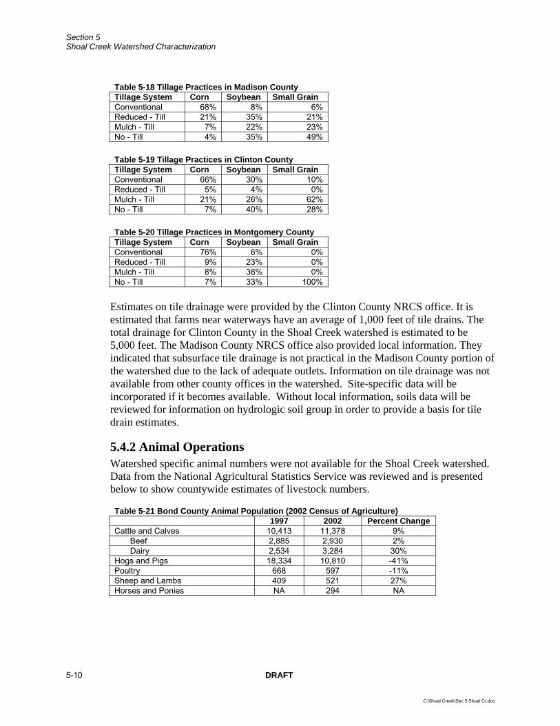
Table 5-18 Tillage Practices in Madison County Tillage System Corn Soybean Small Grain Conventional 68% 8% 6% Reduced - Till 21% 35% 21% Mulch - Till 7% 22% 23% No - Till 4% 35% 49%
Table 5-19 Tillage Practices in Clinton County Tillage System Corn Soybean Small Grain Conventional 66% 30% 10% Reduced - Till 5% 4% 0% Mulch - Till 21% 26% 62% No - Till 7% 40% 28%
Table 5-20 Tillage Practices in Montgomery County Tillage System Corn Soybean Small Grain Conventional 76% 6% 0% Reduced - Till 9% 23% 0% Mulch - Till 8% 38% 0% No - Till 7% 33% 100%
Estimates on tile drainage were provided by the Clinton County NRCS office. It is estimated that farms near waterways have an average of 1,000 feet of tile drains. The total drainage for Clinton County in the Shoal Creek watershed is estimated to be 5,000 feet. The Madison County NRCS office also provided local information. They indicated that subsurface tile drainage is not practical in the Madison County portion of the watershed due to the lack of adequate outlets. Information on tile drainage was not available from other county offices in the watershed. Site-specific data will be incorporated if it becomes available. Without local information, soils data will be reviewed for information on hydrologic soil group in order to provide a basis for tile drain estimates.
5.4.2 Animal Operations Watershed specific animal numbers were not available for the Shoal Creek watershed. Data from the National Agricultural Statistics Service was reviewed and is presented below to show countywide estimates of livestock numbers.
Table 5-21 Bond County Animal Population (2002 Census of Agriculture) 1997 2002 Percent Change Cattle and Calves 10,413 11,378 9% Beef 2,885 2,930 2% Dairy 2,534 3,284 30% Hogs and Pigs 18,334 10,810 -41% Poultry 668 597 -11% Sheep and Lambs 409 521 27% Horses and Ponies NA 294 NA
5-10 DRAFT
C:\Shoal Creek\Sec 5 Shoal Cr.doc

Section 5 Shoal Creek Watershed Characterization
Table 5-22 Madison County Animal Population (2002 Census of Agriculture) 1997 2002 Percent Change Cattle and Calves 17,690 15,809 -11% Beef 5,890 5,931 1% Dairy 1,774 1,683 -5% Hogs and Pigs 46,331 29,844 -36% Poultry 1,517 NA NA Sheep and Lambs 1,047 1,013 -3% Horses and Ponies NA 1,226 NA
Table 5-23 Clinton County Animal Population (2002 Census of Agriculture) 1997 2002 Percent Change Cattle and Calves 37,735 36,849 -2% Beef 5,095 2,242 -56% Dairy 14,830 15,080 2% Hogs and Pigs 93,190 177,880 91% Poultry 552,992 514,945 -7% Sheep and Lambs 473 430 -9% Horses and Ponies NA 402 NA
Table 5-24 Montgomery County Animal Population (2002 Census of Agriculture) 1997 2002 Percent Change Cattle and Calves 13,301 11,053 -17% Beef 4,395 4,212 -4% Dairy 1,082 889 -18% Hogs and Pigs 67,031 58,861 -12% Poultry 2,165 485 -78% Sheep and Lambs 475 388 -18% Horses and Ponies NA 344 NA
Table 5-24 Macoupin County Animal Population (2002 Census of Agriculture) 1997 2002 Percent Change Cattle and Calves 32,393 26,961 -17% Beef 11,188 8,001 -28% Dairy 1,502 1,161 -23% Hogs and Pigs 91,755 68,030 -26% Poultry 1,061 628 -41% Sheep and Lambs 2,190 1,461 -33% Horses and Ponies NA 640 NA
Communications with local NRCS officials have provided more watershed-specific animal information. Clinton County indicated that within the Clinton County portion of the watershed, it is estimated that 21 dairies, seven beef farms, and five hog operations exist. It is estimated that the dairies have an average of 75 to 100 cows while the beef farms range from 25 to 50 head. The hog operations in the area are all likely associated with Mashoff Pork Production. Bond County estimated that three large hog operations existed within that portion of the watershed. In the portion of the watershed located in Montgomery County, it is estimated that there are 11 animal operations. They mostly consist of beef operations and are spread out across that area of the watershed. Madison County estimates that few, if any, animal operations exist in the Madison County area of the watershed.
DRAFT 5-11
C:\Shoal Creek\Sec 5 Shoal Cr.doc

Section 5 Shoal Creek Watershed Characterization
5.5 Watershed Information Previous planning efforts have been conducted within the Shoal Creek watershed. In 1990, a water quality project was completed through Illinois EPA for the Upper Shoal Creek. Communications with local NRCS offices indicated the watershed has been involved in some aspect of EQIP, ERP and State CPP cost-share projects. A 319 water quality project dealing with animal waste projects is also being conducted in the watershed. Further investigation will be performed to determine more information regarding these activities and other watershed groups. Data collected will be reviewed for possible use during Stage 3 of TMDL development.
5-12 DRAFT
C:\Shoal Creek\Sec 5 Shoal Cr.doc

Figure 5-1Water Quality Stations
Shoal Creek Watershed
DRAFT
")
")
")
")
")
")
")
Lake Fork
Breese
PocahontasBe
arca
t Cre
ek
New Douglas
Dry Fork
Dorris Creek
Indian Creek
Little Dry Fork
Shoal Creek
OI 09
SorentoROZH
Locust ForkOIC 02
Cattle CreekOIP 10
Chicken CreekOIO 09
Shoa
l Cre
ekO
I 08
Shoa
l Cre
ekOI
05
§̈¦I-70
tu127
tu140
tu143
tu50
tu161
Mac
oupi
n C
nty
Clinton CntyBond Cnty
Montg om
er y Cnt y
Mad
ison
Cnt
y
Bond C
nty
OI-05
OI-09
OI-08
OIC-02
OIO-09
OIP-10
ROZH-1ROZH-2ROZH-3
0 5 102.5 Miles
{
Legend
InterstateUS and State HighwayRailroadCounty Boundary
WatershedMunicipalityLake or ReservoirMajor Stream303(d) Listed Waterbodies
") Water Quality Station

Section 5 Shoal Creek Watershed Characterization
THIS PAGE INTENTIONALLY LEFT BLANK
5-14 DRAFT
C:\Shoal Creek\Sec 5 Shoal Cr.doc

A
N:\8 Shoal Creek\Data\ShoalCrk Fecal Summary.xlsPLT
Figure 5-2:Shoal Creek Segments OI08 and OI09
Fecal Coliform Samples
1
10
100
1000
10000
100000
Janu
ary-
00
July
-00
Janu
ary-
01
July
-01
Janu
ary-
02
July
-02
Janu
ary-
03
July
-03
Janu
ary-
04
July
-04
Febr
uary
-05
Cou
nt (c
fu/m
L)
OI 08OI 09General Use-200General Use-400Public Water Supply

Section 5 Shoal Creek Watershed Characterization
THIS PAGE INTENTIONALLY LEFT BLANK
5-16 DRAFT
C:\Shoal Creek\Sec 5 Shoal Cr.doc

A
N:\8 Shoal Creek\Data\ShoalCrk Mang&TDS Summary.xlsPLT OI08&09
Figure 5-3:Shoal Creek Segments OI08 and OI09
Total Manganese Samples
0
100
200
300
400
500
600
700
800
900
1000
Janu
ary-
99
July
-99
Janu
ary-
00
July
-00
Dec
embe
r-00
July
-01
Janu
ary-
02
July
-02
Janu
ary-
03
July
-03
Con
cent
ratio
n (u
g/L)
OI 08
OI 09
General Use Standard
Public Water Supply Standard

Section 5 Shoal Creek Watershed Characterization
THIS PAGE INTENTIONALLY LEFT BLANK
5-18 DRAFT
C:\Shoal Creek\Sec 5 Shoal Cr.doc

Figure 5-4NPDES Permits
Shoal Creek Watershed
DRAFT
!(!(
!(!(
!(!(
!(!(
!(!(
!(!(
!(
!(!(
!(!(
!(!(
Lake Fork
Breese
PocahontasBe
arca
t Cre
ek
New Douglas
Dry Fork
Dorris Creek
Indian Creek
Little Dry Fork
Shoa
l Cre
ekO
I 09
SorentoROZH
Locust ForkOIC 02
Cattle CreekOIP 10
Chicken CreekOIO 09
Shoa
l Cre
ekO
I 08
Shoa
l Cre
ekOI
05
§̈¦I-70
£¤127
£¤140
£¤143
£¤50
£¤161
Mac
oupi
n C
nty
Clinton CntyBond Cnty
Montgom
ery Cnty
Mad
ison
Cnt
y Bond C
nty
Western Springs MHP
Breese STP
Sorento WTP
Pierron East STP
Germantown STP
Pocahontas STP
Louisville STP
Sorento STP
New Douglas STP
Panama STP
0 5 102.5 Miles
/
Point Source
Legend
InterstateUS and State HighwayRailroadCounty Boundary
WatershedMunicipality
Lake or ReservoirMajor Stream303(d) Listed Waterbodies

Section 5 Shoal Creek Watershed Characterization
THIS PAGE INTENTIONALLY LEFT BLANK
5-20 DRAFT
C:\Shoal Creek\Sec 5 Shoal Cr.doc

Section 6 Approach to Developing TMDL and Identification of Data Needs Illinois EPA is currently developing TMDLs for pollutants that have numeric water quality standards. Of the pollutants impairing stream segments in the Shoal Creek watershed, DO, fecal coliform, manganese, TDS, silver and copper are all of the parameters with numeric water quality standards. For Sorento Reservoir, manganese is the only parameter with a numeric water quality standard for which a TMDL is being developed. Illinois EPA believes that addressing these impairments should lead to an overall improvement in water quality due to the interrelated nature of the other listed pollutants. Recommended technical approaches for developing TMDLs for streams and lakes are presented in this section. Additional data needs are also discussed.
6.1 Simple and Detailed Approaches for Developing TMDLs The range of analyses used for developing TMDLs varies from simple to complex. Examples of a simple approach include mass-balance, load-duration, and simple watershed and receiving water models. Detailed approaches incorporate the use of complex watershed and receiving water models. Simple approaches typically require less data than detailed approaches and therefore these are the analyses recommended for the Shoal Creek watershed except for stream segments with major point sources whose NDPES permit may be affected by the TMDL's WLA. Establishing a link between pollutant loads and resulting water quality is one of the most important steps in developing a TMDL. As discussed above, this link can be established through a variety of techniques. The objective of the remainder of this section is to recommend approaches for establishing these links for the constituents of concern in the Shoal Creek watershed.
6.2 Approaches for Developing TMDLs for Stream Segments in the Shoal Creek Watershed Stream segments with major point sources (those discharging greater than 0.1 million gallons per day) in the Shoal Creek watershed are segments OI08 and OI05 of Shoal Creek. The remaining impaired segments do not have major point sources discharging to them. Approaches for developing TMDLs for areas with and without major point sources are described below.
6.2.1 Recommended Approach for DO TMDLs for Stream Segments without Major Point Sources Locust Creek, Cattle Creek, and Chicken Creek do not have major point sources discharging to them and are all listed as impaired for DO. Cattle Creek is also listed as impaired for total ammonia nitrogen. The data for these segments are limited and it is suggested that these segments proceed to Stage 2 in order to obtain more information for modeling. Once data collection has occurred, a simplified approach that involves
DRAFT 6-1
C:\Shoal Creek\Sec 6 Shoal Cr.doc

Section 6 Approach to Developing TMDL and Identification of Data Needs
simulating pollutant oxidation and stream reaeration only within a spreadsheet model is recommended for these TMDLs. The model simulates steady-state stream DO as a function of carbonaceous and nitrogenous pollutant oxidation and atmospheric reaeration. The model allows for non-uniform stream hydraulics, hydrology, and pollutant loadings at any level of segmentation. It is also free of numerical dispersion as it relies on well-known analytical solutions rather than numerical approximations of the fundamental equations. The model assumes plug flow (no hydrodynamic dispersion), which is likely an acceptable assumption for most small to medium sized streams. The model also does not incorporate the impacts of stream plant life, which generally require site-specific data for meaningful parameterization. A toxicitiy component will be incorporated for the total ammonia calculations. A watershed model will not be used for these segments. Using the spreadsheet model iteratively, the BOD loads causing the impairments and that are required to maintain a DO concentration of 5.0 mg/L will be calculated. These calculated loads will become the basis for recommending TMDL reductions if necessary.
6.2.2 Recommended Approach for DO TMDLs for Segments with Major Point Sources The Germantown STP discharges above Shoal Creek segment OI05. For this segment a more complicated approach that would also incorporate the impacts of stream plant activity, and possibly sediment oxygen demand (SOD), and would require a more sophisticated numerical model and an adequate level of measured data to aide in model parameterization is recommended.
Available instream water quality data for this segement are limited to three samples. Data are also very limited spatially. Therefore, additional data collection is recommended for this segment. Specific data requirements include a synoptic (snapshot in time) water quality survey of this reach with careful attention to the location of the point source dischargers. This survey should include measurements of flow, hydraulics, DO, temperature, nutrients, and CBOD. The collected data will be used to support the model development and parameterization and will lend significant confidence to the TMDL conclusions.
This newly collected data could then be used to support the development and parameterization of a more sophisticated DO model for this stream and therefore, the use of the QUAL2E model (Brown and Barnwell 1985) could be utilized to accomplish the TMDL analysis for Shoal Creek. QUAL2E is well-known and USEPA-supported. It simulates DO dynamics as a function of nitrogenous and carbonaceous oxygen demand, atmospheric reaeration, SOD, and phytoplankton photosynthesis and respiration. The model also simulates the fate and transport of nutrients and BOD and the presence and abundance of phytoplankton (as chlorophyll-a). Stream hydrodynamics and temperature are important controlling parameters in the model. The model is essentially only suited to steady-state simulations.
In addition to the QUAL2E model, a simple watershed model such as PLOAD, Unit Area Loads or the Watershed Management Model is recommended to estimated BOD
6-2 DRAFT
C:\Shoal Creek\Sec 6 Shoal Cr.doc

Section 6 Approach to Developing TMDL and Identification of Data Needs
and nutrient loads from non-point sources in the watershed. This model will allow for allocation between point and nonpoint source loads and provide an understanding of percentage of loadings from point sources and nonpoint sources in the watershed.
6.2.3 Recommended Approach for Fecal Coliform TMDLs Segments OI08 and OI09 of Shoal Creek are listed as impaired for total fecal coliform. The recommend approach for developing a TMDL for these segments is use of the load-duration curve method. The load-duration methodology uses the cumulative frequency distribution of streamflow and pollutant concentration data to estimate the allowable loads for a waterbody.
6.2.4 Recommended Approach for Manganese, TDS, and Metal TMDLs in Non-Mining Impacted Areas Segments OI08 and OI09 of Shoal Creek and OIC02 of Locust Creek are impaired for manganese. Cattle Creek is impaired for TDS and copper while Chicken Creek is impaired for silver. Segments OI08 and OI09 of Shoal Creek have adequate manganese data for TMDL development, however, limited data are available for the remaining segments and parameters. It is recommended that more data be collected on Locust, Cattle, and Chicken Creeks. No apparent sources of manganese, TDS, or metals have been identified to date. Once adequate data is available for each of the parameters and segments, an empirical loading and spreadsheet analysis will be utilized to calculate these TMDLs.
6.3 Approaches for Developing a TMDL for Sorento Reservoir The recommended TMDL approach for Sorento Reservoir will be discussed in this section. It is assumed that enough data exists to develop a simple model for use in TMDL development.
6.3.1 Recommended Approach for Manganese TMDL The applicable water quality standard for manganese is 150 µg/L. The reservoir is also listed for a phosphorus impairment, but the standard does not apply to reservoirs with a surface area less than 20 acres. However, it is assumed that development of a phosphorus TMDL will control the manganese concentrations. The manganese target is maintenance of hypolimnetic DO concentrations above zero, because the only controllable source of manganese to the lake is the release of manganese from lake sediments during periods when there is no DO in lake bottom waters. The lack of DO in lake bottom waters is presumed to be due to the effects of nutrient enrichment, as there are no significant sources of oxygen demanding materials to the lake. For this reason, attainment of the total phosphorus standard is expected to result in oxygen concentrations that will reduce sediment manganese flux to natural background levels. The TMDL target is therefore set as a total phosphorus concentration of 0.050 mg-P/l.
DRAFT 6-3
C:\Shoal Creek\Sec 6 Shoal Cr.doc
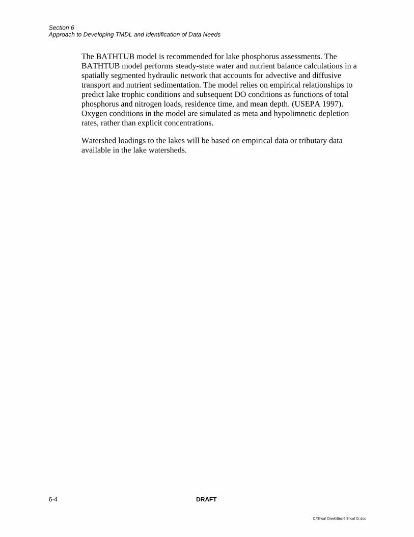
Section 6 Approach to Developing TMDL and Identification of Data Needs
The BATHTUB model is recommended for lake phosphorus assessments. The BATHTUB model performs steady-state water and nutrient balance calculations in a spatially segmented hydraulic network that accounts for advective and diffusive transport and nutrient sedimentation. The model relies on empirical relationships to predict lake trophic conditions and subsequent DO conditions as functions of total phosphorus and nitrogen loads, residence time, and mean depth. (USEPA 1997). Oxygen conditions in the model are simulated as meta and hypolimnetic depletion rates, rather than explicit concentrations.
Watershed loadings to the lakes will be based on empirical data or tributary data available in the lake watersheds.
6-4 DRAFT
C:\Shoal Creek\Sec 6 Shoal Cr.doc

TMDL Development for the Shoal Creek Watershed, Illinois
FINAL REPORT FOR USEPA APPROVAL
August 30, 2007
Illinois Environmental Protection Agency

TMDL Development for the Shoal Creek Watershed, Illinois
FINAL REPORT FOR USEPA APPROVAL
August 30th, 2007
Submitted to: Illinois Environmental Protection Agency
1021 N. Grand Avenue East Springfield, IL 62702
Submitted by: Tetra Tech, Inc.
Water Resources TMDL Center
.

Illinois Environmental Protection Agency TMDL Development for the Shoal Creek Watershed
Final Report for USEPA Approval i
TABLE OF CONTENTS 1.0 Introduction................................................................................................................................................ 1 2.0 Background................................................................................................................................................ 2 3.0 Applicable Water Quality Standards......................................................................................................... 6
3.1 Use Support Guidelines ................................................................................................................. 6 4.0 Technical Analysis .................................................................................................................................... 8
4.1 Load Duration Curves.................................................................................................................... 8 4.1.1 Stream Flow Estimates............................................................................................................ 10
4.2 QUAL2K Model .......................................................................................................................... 12 5.0 TMDL ...................................................................................................................................................... 13
5.1 Loading Capacity for Fecal Coliform, Manganese, Silver, Ammonia, Copper, and TDS in the Shoal Creek Watershed ............................................................................................................................. 13
5.1.1 Loading Capacity of Shoal Creek Segment OI08 .................................................................. 13 5.1.2 Loading Capacity of Shoal Creek Stream Segment OI09...................................................... 15 5.1.3 Loading Capacity of Chicken Creek Stream Segment OIO09............................................... 16 5.1.4 Loading Capacity of Cattle Creek Stream Segment OIP10 ................................................... 17 5.1.5 Waste Load Allocations .......................................................................................................... 18 5.1.6 Load Allocation ....................................................................................................................... 19 5.1.7 Margin of Safety...................................................................................................................... 19 5.1.8 Critical Conditions and Seasonality........................................................................................ 20
5.2 Dissolved Oxygen in the Shoal Creek Watershed ...................................................................... 20 5.2.1 Dissolved Oxygen Analysis in Locust Fork ........................................................................... 20 5.2.2 Dissolved Oxygen Analysis in Cattle Creek .......................................................................... 21 5.2.3 Dissolved Oxygen Analysis in Chicken Creek....................................................................... 22
References...................................................................................................................................................... 24 Appendix A : Load Duration Analysis .......................................................................................................A-1 Appendix B : Fecal Coliform, Manganese, Silver, TDS, Copper, and Ammonia Data for Load Duration Analysis........................................................................................................................................................ B-1 Appendix C : NPDES Fecal Coliform Counts............................................................................................ C-1 Appendix D : QUAL2K Modeling .............................................................................................................D-1 Appendix E : Stage 1 Report ....................................................................................................................... E-1 Appendix F : Stage 2 Report ........................................................................................................................F-1

Illinois Environmental Protection Agency TMDL Development for the Shoal Creek Watershed
Final Report for USEPA Approval i
FIGURES Figure 1. Location of the Shoal Creek Watershed ................................................................................... 4 Figure 2. Land Use in the Shoal Creek Watershed .................................................................................. 5 Figure 3. USGS and Load Duration Stations in the Shoal Creek Watershed........................................ 11 TABLES Table 1. Section 303(d) listed waterbodies within the Shoal Creek watershed addressed within this report........................................................................................................................ 3 Table 2. Summary of Water Quality Standards for the Shoal Creek Watershed Stream Impairments. 7 Table 3. 303(d) List Information and Modeling Approaches for the Shoal Creek Watershed ............. 8 Table 4. Relationship Between Load Duration Curve Zones and Contributing Sources. ................... 10 Table 5. Fecal Coliform and Manganese TMDL Summary for Stream Segment OI08 ...................... 14 Table 6. Fecal Coliform and Manganese TMDL Summary for Stream Segment OI09 ...................... 16 Table 7. Silver TMDL Summary for Stream Segment OIO09............................................................. 17 Table 8. TDS, Copper, and Ammonia TMDL Summary for Stream Segment OIP10 ........................ 18 Table 9. Fecal Coliform Limits and WLA for NPDES Facilities in the Shoal Creek watershed........ 19 Table 10. Pollutant load reductions needed for Locust Fork to achieve dissolved oxygen criteria. ..... 21 Table 11. Pollutant load reductions needed for Cattle Creek to achieve dissolved oxygen criteria. .... 22 Table 12. Pollutant load reductions needed for Chicken Creek to achieve dissolved oxygen criteria.. 23

Illinois Environmental Protection Agency TMDL Development for the Shoal Creek Watershed
Final Report for USEPA Approval 1
1.0 INTRODUCTION A TMDL is defined as “the sum of the individual wasteload allocations for point sources and load allocations for nonpoint sources and natural background” such that the capacity of the waterbody to assimilate pollutant loadings is not exceeded. A TMDL is also required to be developed with seasonal variations and must include a margin of safety that addresses the uncertainty in the analysis. The overall goals and objectives in developing TMDLs for the above listed waterbodies include:
• Assess the water quality of the impaired waterbodies and identify key issues associated with the impairments and potential pollutant sources.
• Use the best available science and available data to determine the maximum load the waterbodies
can receive and fully support all of their designated uses.
• Use the best available science and available data to determine current loads of pollutants to the impaired waterbodies.
• If current loads exceed the maximum allowable load, determine the load reduction that is needed.
• Identify feasible and cost-effective actions that can be taken to reduce loads.
• Inform and involve the public throughout the project to ensure that key concerns are addressed
and the best available information is used.
• Submit a final TMDL report to USEPA for review and approval. The Illinois Environmental Protection Agency (IEPA) has a three-stage approach to total maximum daily load (TMDL) development. The stages are:
Stage 1 was completed by the consulting firm Camp Dresser and McKee (CDM) in October 2006 and involved characterization of the watershed, assessment of the available water quality data, identification of additional data needs for the development of credible TMDLs and recommendation of potential technical approaches for TMDL development (Appendix E).
Stage 2 was also completed by the CDM consulting firm in March 2007 and involved collecting
additional chemical water quality data, continuous dissolved oxygen measurements, channel morphology and discharge measurements at twenty-five monitoring locations (Figure 1 and Appendix F).
Stage 3 was completed by the Tetra Tech consulting firm and involves model development and
calibration, TMDL scenarios, and implementation planning. This report documents the modeling and TMDL components of Stage 3. The specific pollutant sources were not a focus of this report and will be the subject of a forthcoming Implementation Plan, along with a description of alternatives for achieving the desired load reductions.

Illinois Environmental Protection Agency TMDL Development for the Shoal Creek Watershed
Final Report for USEPA Approval 2
2.0 BACKGROUND The Shoal Creek watershed has a drainage area of approximately 921 square miles and is an 8 digit hydrologic unit code (07140203) as defined by USGS Geological Survey (USGS). The watershed is located in south-central Illinois and the portion of the watershed addressed in this report has a drainage area of 310 square miles and encompasses five counties with Bond County covering 46 percent of the watershed followed by Montgomery (28%), Clinton (23%), Madison (3%), and Macoupin (0.05%)(Figure 1). The Shoal Creek headwaters begin in north-eastern Montgomery County and continue south towards the Kaskaskia River. Major tributaries to Shoal Creek include the West, Middle, and East Forks of Shoal Creek and Beaver Creek. Agriculture is the dominant land use in this watershed (Figure 2). Table 1 lists the Shoal Creek watershed Section 303(d) listing information along with an identification of the TMDLs presented in this report. IEPA is currently developing TMDLs only for pollutants that have numeric water quality standards. However, best management practices identified for pollutants with numeric water quality standards (e.g., copper, silver) might include the control of other pollutants (e.g., suspended solids) that do not have water quality standards. Information on these potential best management practices will be forthcoming in the implementation plan. Several segments have been de-listed since the Stage 1 report due to newer ambient data or data collected during Stage 2. Shoal Creek was originally listed as impaired for dissolved oxygen. However, additional data collected in 2006 indicated no exceedances of the dissolved oxygen water quality standard (Appendix F). USEPA has therefore already approved a de-listing of dissolved oxygen for segment OI05 of Shoal Creek and no TMDL has been developed. Locust Fork was originally listed as impaired for manganese. However, additional data collected in 2006 indicated no exceedances of the manganese water quality standard. USEPA has therefore already approved a de-listing of manganese for the OIC01 segment of Locust Fork and no TMDL has been developed. Sorento Lake was originally listed as impaired for manganese but it was later determined that was in error due to the fact the lake is not designated as a public water supply. No TMDL has therefore been developed for Sorento Lake.

Illinois Environmental Protection Agency TMDL Development for the Shoal Creek Watershed
Final Report for USEPA Approval 3
Table 1. Section 303(d) listed waterbodies within the Shoal Creek watershed addressed within this report.
Waterbody Name
Waterbody Segment
Segment Size
(Miles) Cause of Impairment Impaired Designated Use
Fecal Coliform Primary Contact Recreation Shoal Creek OI-08 13.11
Manganese Public Water Supplies
Fecal Coliform Primary Contact Recreation Shoal Creek OI-09 29.75
Manganese Public Water Supplies Dissolved Oxygen Aquatic Life Total Phosphorus Aquatic Life Sedimentation/Siltation Aquatic Life
Locust Fork OIC-02 4.24
Total Suspended Solids Aquatic Life Dissolved Oxygen Aquatic Life Silver Aquatic Life Total Nitrogen Aquatic Life Total Phosphorus Aquatic Life Sedimentation/Siltation Aquatic Life
Chicken Creek OIO-09 1.92
Total Suspended Solids Aquatic Life Ammonia Aquatic Life Copper Aquatic Life Dissolved Oxygen Aquatic Life TDS Aquatic Life Total Phosphorus Aquatic Life Sedimentation/Siltation Aquatic Life
Cattle Creek OIP-10 2.71
Total Suspended Solids Aquatic Life Note: Bold font indicates cause will be addressed in this report because there are numeric water quality criteria.

Illinois Environmental Protection Agency TMDL Development for the Shoal Creek Watershed
Final Report for USEPA Approval 4
Figure 1. Location of the Shoal Creek Watershed

Illinois Environmental Protection Agency TMDL Development for the Shoal Creek Watershed
Final Report for USEPA Approval 5
Figure 2. Land Use in the Shoal Creek Watershed
Illinois Environmental Protection Agency TMDL Development for the Shoal Creek Watershed
Final Report for USEPA Approval 6
3.0 APPLICABLE WATER QUALITY STANDARDS The purpose of developing a TMDL is to identify the pollutant loading that a waterbody can receive and still achieve water quality standards. Under the Clean Water Act, every state must adopt water quality standards to protect, maintain, and improve the quality of the nation’s surface waters. These standards represent a level of water quality that will support the Clean Water Act’s goal of “swimmable/fishable” waters. Water quality standards consist of three components: designated uses, numeric or narrative criteria, and an antidegradation policy. A description of the water quality standards that apply to this TMDL is presented below and detailed comparisons of the available water quality data to the standards are provided in Appendix E and Appendix F. 3.1 Use Support Guidelines IEPA uses rules and regulations adopted by the Illinois Pollution Control Board (IPCB) to assess the designated use support for Illinois waterbodies. The following are the use support designations provided by the IPCB that apply to water bodies in the Shoal Creek watershed: General Use Standards - These standards protect for aquatic life, wildlife, agricultural, primary contact (where physical configuration of the waterbody permits it, any recreational or other water use in which there is prolonged and intimate contact with the water involving considerable risk of ingesting water in quantities sufficient to pose a significant health hazard, such as swimming and water skiing), secondary contact (any recreational or other water use in which contact with the water is either incidental or accidental and in which the probability of ingesting appreciable quantities of water is minimal, such as fishing, commercial and recreational boating, and any limited contact incident to shoreline activity), and most industrial uses. These standards are also designed to ensure the aesthetic quality of the state's aquatic environment. Public and food processing water supply standards – These standards are cumulative with the general use standards and apply to waters of the state at any point at which water is withdrawn for treatment and distribution as a potable supply to the public or for food processing. Water quality standards used for TMDL development in the Shoal Creek watershed are listed below in Table 2.
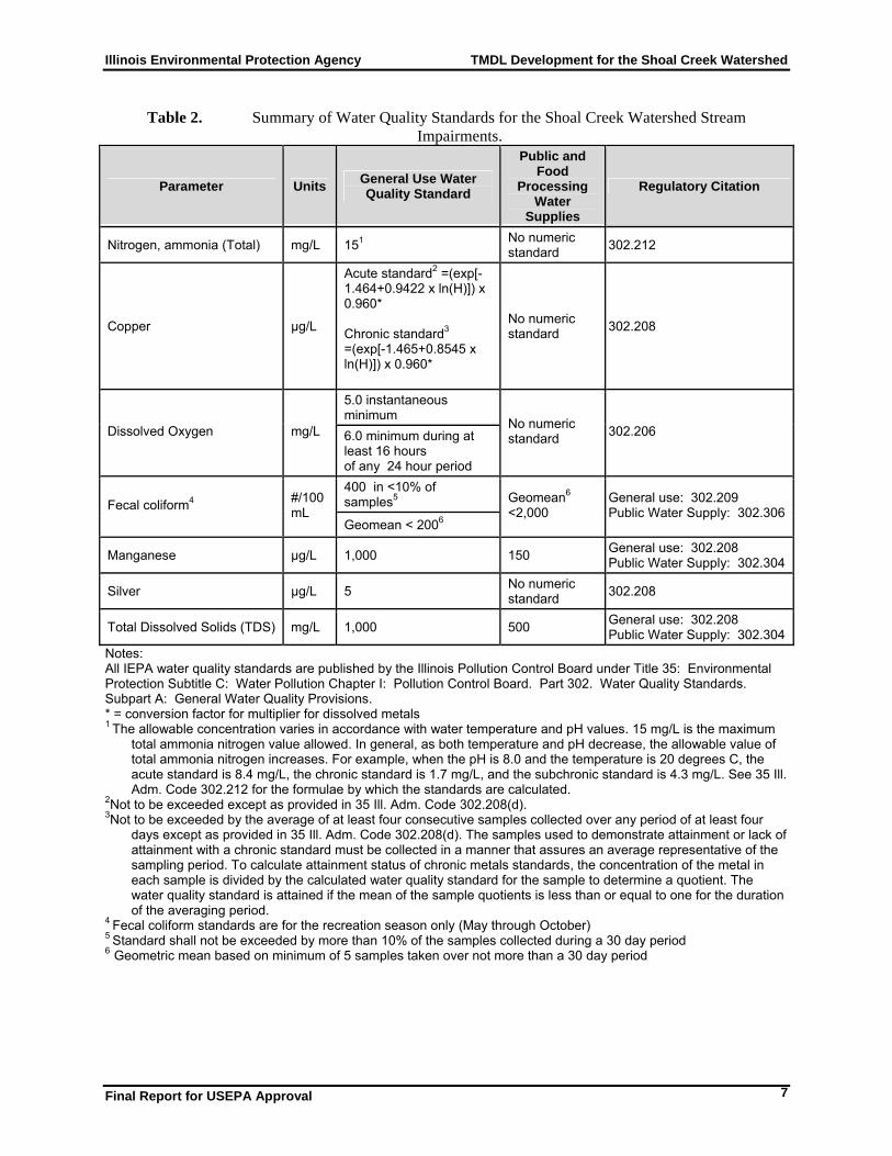
Illinois Environmental Protection Agency TMDL Development for the Shoal Creek Watershed
Final Report for USEPA Approval 7
Table 2. Summary of Water Quality Standards for the Shoal Creek Watershed Stream Impairments.
Parameter Units General Use Water Quality Standard
Public and Food
Processing Water
Supplies
Regulatory Citation
Nitrogen, ammonia (Total) mg/L 151 No numeric standard 302.212
Copper µg/L
Acute standard2 =(exp[-1.464+0.9422 x ln(H)]) x 0.960* Chronic standard3 =(exp[-1.465+0.8545 x ln(H)]) x 0.960*
No numeric standard 302.208
5.0 instantaneous minimum
Dissolved Oxygen mg/L 6.0 minimum during at least 16 hours of any 24 hour period
No numeric standard 302.206
400 in <10% of samples5 Fecal coliform4 #/100
mL Geomean < 2006
Geomean6
<2,000 General use: 302.209 Public Water Supply: 302.306
Manganese µg/L 1,000 150 General use: 302.208 Public Water Supply: 302.304
Silver µg/L 5 No numeric standard 302.208
Total Dissolved Solids (TDS) mg/L 1,000 500 General use: 302.208 Public Water Supply: 302.304
Notes: All IEPA water quality standards are published by the Illinois Pollution Control Board under Title 35: Environmental Protection Subtitle C: Water Pollution Chapter I: Pollution Control Board. Part 302. Water Quality Standards. Subpart A: General Water Quality Provisions. * = conversion factor for multiplier for dissolved metals 1 The allowable concentration varies in accordance with water temperature and pH values. 15 mg/L is the maximum
total ammonia nitrogen value allowed. In general, as both temperature and pH decrease, the allowable value of total ammonia nitrogen increases. For example, when the pH is 8.0 and the temperature is 20 degrees C, the acute standard is 8.4 mg/L, the chronic standard is 1.7 mg/L, and the subchronic standard is 4.3 mg/L. See 35 Ill. Adm. Code 302.212 for the formulae by which the standards are calculated.
2Not to be exceeded except as provided in 35 Ill. Adm. Code 302.208(d). 3Not to be exceeded by the average of at least four consecutive samples collected over any period of at least four
days except as provided in 35 Ill. Adm. Code 302.208(d). The samples used to demonstrate attainment or lack of attainment with a chronic standard must be collected in a manner that assures an average representative of the sampling period. To calculate attainment status of chronic metals standards, the concentration of the metal in each sample is divided by the calculated water quality standard for the sample to determine a quotient. The water quality standard is attained if the mean of the sample quotients is less than or equal to one for the duration of the averaging period.
4 Fecal coliform standards are for the recreation season only (May through October)
5 Standard shall not be exceeded by more than 10% of the samples collected during a 30 day period 6 Geometric mean based on minimum of 5 samples taken over not more than a 30 day period
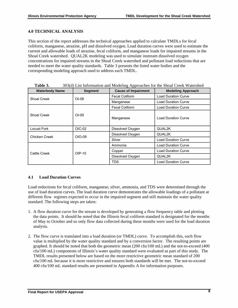
Illinois Environmental Protection Agency TMDL Development for the Shoal Creek Watershed
Final Report for USEPA Approval 8
4.0 TECHNICAL ANALYSIS This section of the report addresses the technical approaches applied to calculate TMDLs for fecal coliform, manganese, atrazine, pH and dissolved oxygen. Load duration curves were used to estimate the current and allowable loads of atrazine, fecal coliform, and manganese loads for impaired streams in the Shoal Creek watershed. QUAL2K modeling was used to simulate instream dissolved oxygen concentrations for impaired streams in the Shoal Creek watershed and pollutant load reductions that are needed to meet the water quality standards. Table 3 presents the listed water bodies and the corresponding modeling approach used to address each TMDL.
Table 3. 303(d) List Information and Modeling Approaches for the Shoal Creek Watershed Waterbody Name Segment Cause of Impairment Modeling Approach
Fecal Coliform Load Duration Curve Shoal Creek OI-08
Manganese Load Duration Curve Fecal Coliform Load Duration Curve
Shoal Creek OI-09 Manganese Load Duration Curve
Locust Fork OIC-02 Dissolved Oxygen QUAL2K
Dissolved Oxygen QUAL2K Chicken Creek OIO-09
Silver Load Duration Curve Ammonia Load Duration Curve Copper Load Duration Curve Dissolved Oxygen QUAL2K
Cattle Creek OIP-10
TDS Load Duration Curve 4.1 Load Duration Curves Load reductions for fecal coliform, manganese, silver, ammonia, and TDS were determined through the use of load duration curves. The load duration curve demonstrates the allowable loadings of a pollutant at different flow regimes expected to occur in the impaired segment and still maintain the water quality standard. The following steps are taken: 1. A flow duration curve for the stream is developed by generating a flow frequency table and plotting
the data points. It should be noted that the Illinois fecal coliform standard is designated for the months of May to October and so only flow data collected during these months were used for the load duration analysis.
2. The flow curve is translated into a load duration (or TMDL) curve. To accomplish this, each flow
value is multiplied by the water quality standard and by a conversion factor. The resulting points are graphed. It should be noted that both the geometric mean (200 cfu/100 mL) and the not-to-exceed (400 cfu/100 mL) components of Illinois’s water quality standard were evaluated as part of this study. The TMDL results presented below are based on the more restrictive geometric mean standard of 200 cfu/100 mL because it is more restrictive and ensures both standards will be met. The not-to-exceed 400 cfu/100 mL standard results are presented in Appendix A for information purposes.

Illinois Environmental Protection Agency TMDL Development for the Shoal Creek Watershed
Final Report for USEPA Approval 9
3. Each water quality sample is converted to a load by multiplying the water quality sample concentration by the average daily flow on the day the sample was collected and a conversion factor. Then, the individual loads are plotted on the TMDL graph.
4. Points plotting above the curve represent deviations from the water quality standard and the daily
allowable load. Those plotting below the curve represent compliance with standards and the daily allowable load.
5. The area beneath the TMDL curve is interpreted as the loading capacity of the stream. The difference
between this area and the area representing the current loading conditions is the load that must be reduced to meet water quality standards.
Fecal coliform and total manganese loadings were calculated for Shoal Creek segments OI08 and OI09. Segment OI08 starts at the confluence of Shoal Creek and Cattle Creek and ends at the confluence of Beaver Creek. Segment OI09 begins downstream of the confluence of the West and Middle Forks of Shoal Creek and ends at the confluence with the East Fork of Shoal Creek (Figure 3). Allowable silver loads were calculated for Chicken Creek segment OIO09 that covers the entire length of Chicken Creek from the headwaters to the mouth (Figure 3). Ammonia, copper and TDS loadings were calculated for the OIP10 segment of Cattle Creek. This segment covers the entire mainstem of Cattle Creek from the headwaters to the mouth (Figure 3). Fecal coliform and total manganese data for sampling stations OI08 and OI09 were used to assess loadings to segments OI08 and OI09, silver data for sampling station OIO09 were used to assess loadings to segment OIO09, and ammonia, copper, and TDS data for sampling station OIP10 were used to assess loadings to segment OIP10. The pollutant reductions necessary to achieve the applicable water quality standards are presented in Section 5.1. The stream flows displayed on a load duration curve may be grouped into various flow regimes to aid with interpretation of the load duration curves. The flow regimes are typically divided into 10 groups, which can be further categorized into the following five “hydrologic zones” (Cleland, 2005):
• High flow zone: stream flows that plot in the 0 to 10-percentile range, related to flood flows. • Moist zone: flows in the 10 to 40-percentile range, related to wet weather conditions. • Mid-range zone: flows in the 40 to 50 percentile range, median stream flow conditions; • Dry zone: flows in the 60 to 90-percentile range, related to dry weather flows. • Low flow zone: flows in the 90 to 100-percentile range, related to drought conditions.
The load duration approach helps to identify the issues surrounding the impairment and to roughly differentiate between sources. Table 4 summarizes the relationship between the five hydrologic zones and potentially contributing source areas. The load reduction approach also considers critical conditions and seasonal variation in the TMDL development as required by the Clean Water Act and EPA’s implementing regulations. Because the approach establishes loads based on a representative flow regime, it inherently considers seasonal variations and critical conditions attributed to flow conditions.

Illinois Environmental Protection Agency TMDL Development for the Shoal Creek Watershed
Final Report for USEPA Approval 10
Table 4. Relationship Between Load Duration Curve Zones and Contributing Sources.
Duration Curve Zone
Contributing Source Area High Moist Mid-Range Dry Low
Point source M H Livestock direct access to streams M H On-site wastewater systems M M-H H H H Riparian areas H H M Stormwater: Impervious H H H Combined sewer overflow (CSO) H H H Stormwater: Upland H H M Field drainage: Natural condition H M Field drainage: Tile system H H M-H L-M Bank erosion H M Note: Potential relative importance of source area to contribute loads under given hydrologic condition (H: High; M: Medium; L: Low)
4.1.1 Stream Flow Estimates Daily stream flows are needed to apply the load duration curve. There is one USGS gage station with continuous flow data in the Shoal Creek watershed (Figure 3). USGS station 05594000 is located near Breese, Illinois on the OI08 segment of Shoal Creek. Stream flows for all monitoring stations (OI08, OI09, OIO09, and OIP10) were extrapolated from the USGS station 05594000, using a multiplier based upon a comparison of the two drainage areas. For example, the drainage area upstream of the OI08 monitoring station is 725.82 square miles and the drainage area upstream of the USGS gage station is 735 square miles. The drainage area ratio therefore equals 0.9875 and the daily flows at the flow gage were multiplied by 0.9875 to estimate the daily flows at station OI08. A further modification to the flow estimates was made to ensure that they accounted for the design flows of any upstream point sources (because the TMDL WLAs are based on design flows). In cases where the minimum estimated flows were less than the cumulative design flows of upstream point sources, the design flows were added to the flow record.

Illinois Environmental Protection Agency TMDL Development for the Shoal Creek Watershed
Final Report for USEPA Approval 11
Figure 3. USGS and Load Duration Stations in the Shoal Creek Watershed

Illinois Environmental Protection Agency TMDL Development for the Shoal Creek Watershed
Final Report for USEPA Approval 12
4.2 QUAL2K Model The QUAL2K water quality model was used to assess dissolved oxygen concentrations in Locust Fork, Cattle Creek, and Chicken Creek. QUAL2K is supported by U.S. EPA and has been used extensively for TMDL development and point source permitting issues across the country, especially for issues related to dissolved oxygen concentrations. The QUAL2K model is suitable for simulating hydraulics and water quality conditions of a small river. It is a one-dimensional model with the assumption of a completely mixed system for each computational cell. QUAL2K assumes that the major pollutant transport mechanisms, advection and dispersion, are significant only along the longitudinal direction of flow. The model allows for multiple waste discharges, water withdrawals, tributary flows, and incremental inflows and outflows. The processes employed in QUAL2K address nutrient cycles, algal growth, and dissolved oxygen dynamics.

Illinois Environmental Protection Agency TMDL Development for the Shoal Creek Watershed
Final Report for USEPA Approval 13
5.0 TMDL A TMDL is the total amount of a pollutant that can be assimilated by the receiving water while still achieving water quality standards. TMDLs can be expressed in terms of mass per time or by other appropriate measures. TMDLs are composed of the sum of individual wasteload allocations (WLAs) for point sources and load allocations (LAs) for nonpoint sources (including natural background levels). In addition, the TMDL must include a margin of safety (MOS), either implicitly or explicitly, that accounts for the uncertainty in the relationship between pollutant loads and the quality of the receiving waterbody. Conceptually, this is defined by the equation:
TMDL = 'WLAs + 'LAs + MOS A summary of the TMDL allocations for the Shoal Creek watershed is presented in this section of the report, organized according to pollutants and modeling analysis. 5.1 Loading Capacity for Fecal Coliform, Manganese, Silver, Ammonia, Copper, and TDS in the
Shoal Creek Watershed A TMDL must identify the loading capacity of a waterbody for the applicable pollutant. USEPA regulations define loading capacity as the greatest amount of a pollutant that a waterbody can receive without violating water quality standards. The loading capacity is often referred to as the “allowable” load. The following sections provide load duration curve analysis for Segments OI08, OI09, OIO09, and OIP10 of Shoal Creek. Table 5 lists the fecal coliform and manganese load reductions needed at Shoal Creek segment OI08, Table 6 lists the fecal coliform and manganese load reductions needed at Shoal Creek segment OI09, Table 7 lists the silver load reductions needed in Chicken Creek, and Table 8 lists the ammonia, copper, and TDS load reductions needed in Cattle Creek. Appendix A presents the detailed load duration analyses performed for Shoal Creek at stations OI08, OI09, OIO09, and OIP10. 5.1.1 Loading Capacity of Shoal Creek Segment OI08 Existing and allowable fecal coliform and manganese loads were calculated for Shoal Creek segment OI08 at station OI08 located at the Route 50 bridge, 1.4 miles east of Breese. This location drains 726 square miles and land use/land cover consists primarily of cultivated crops, deciduous forest, and pasture/hay. Numerous livestock operations are located within the Shoal Creek watershed upstream of and adjacent to this segment. A total of 39 fecal coliform samples and 41 manganese samples were available for the load duration analysis (Appendix B). The TMDL summary for Shoal Creek segment OI08 is presented in Table 5. Current observed loads for each flow regime are based on the median observed flow in each regime and the results indicate that fecal coliform observations exceed the loading limit most frequently between very high and mid range flows. Manganese loadings are above the threshold loadings throughout the entire flow range with 46 percent or greater needed reductions.

Illinois Environmental Protection Agency TMDL Development for the Shoal Creek Watershed
Final Report for USEPA Approval 14
Table 5. Fecal Coliform and Manganese TMDL Summary for Stream Segment OI08
OI08 TMDL High Flows Moist Conditions
Mid-Range Flows
Dry Conditions
Low Flows
Pollutant TMDL Component 0-10 10-40 40-60 60-90 90-100 Current Load 125,343,030 4,899,685 486,344 124,123 No Data TMDL= LA+WLA+MOS 7,972,860 995,400 285,090 111,137 40,589 LA 7,945,378 967,918 257,608 97,903 27,355 WLA: Pierron East STP 156 156 156 156 156 WLA: Breese STP 23,772 23,772 23,772 9,524 9,524 WLA: Louisville STP 1,136 1,136 1,136 1,136 1,136 WLA: Pocahontas STP 946 946 946 946 946 WLA: Panama STP 397 397 397 397 397 WLA: New Douglas STP 416 416 416 416 416 WLA: Sorento STP 530 530 530 530 530 WLA Sorento WTP 129 129 129 129 129 WLA: MS4 n/a n/a n/a n/a n/a WLA: Total Point Sources 27,482 27,482 27,482 13,234 13,234 MOS (Implicit) Implicit Implicit Implicit Implicit Implicit
Fecal Coliform (Million/day)
TMDL Reduction (%) 94% 80% 41% 10% No Data Current Load 3,182.6 330.7 71.0 30.2 7.6 TMDL= LA+WLA+MOS 1,080.0 156.6 42.4 13.4 3.6 LA 972.0 140.9 38.2 12.1 3.2
Future Growth Reserve (0%) 0.0 0.0 0.0 0.0 0.0 WLA: facility n/a n/a n/a n/a n/a WLA: MS4 n/a n/a n/a n/a n/a MOS (10%) 108.0 15.7 4.2 1.3 0.4
Manganese (kg/day)
TMDL Reduction (%) 69% 57% 46% 60% 57% The following sewage treatment plants (STP) are located in the Shoal Creek watershed upstream of monitoring station OI08:
Pierron East STP (permit number ILG580237) Breese STP (permit number IL0022772) Louisville STP (permit number ILG580081) Pocahontas STP(permit number ILG580010) Panama STP (permit number IL0048992) New Douglas STP (permit number IL0074292) Sorento STP (permit number ILG580049) Sorento WTP (permit number ILG640149)
Sewage from treatment plants treating domestic and/or municipal waste contains fecal coliform–it is indigenous to sanitary sewage. All facilities addressed by this TMDL, with the exception of the Breese STP, have applied for and received disinfection exemptions which allow the facility to discharge wastewater water without disinfection. All of these treatment facilities are required to comply with the geometric mean fecal coliform water quality standard of 200 cfu/100 mL at the closest point downstream where recreational use occurs in the receiving water. The WLAs shown Table 5 were therefore calculated

Illinois Environmental Protection Agency TMDL Development for the Shoal Creek Watershed
Final Report for USEPA Approval 15
based on the facility design flows multiplied by 200 cfu/100 mL for the facilities with disinfection exemptions. Facilities with year-round disinfection exemptions may be required to provide the Agency with updated information to demonstrate compliance with these requirements. Facilities directly discharging into a fecal-impaired segment may have their year-round disinfection exemption revoked through future NPDES permitting actions. The WLAs for the Breese STP facility were determined by multiplying the facility’s design maximum flow (DMF) by its permit limit (400/100 mL) during high to mid range flows and by multiplying the design average flow (DAF) by the permit limit during low flows and moist conditions. Monitoring data from this facility indicate that the effluent is well within its permit limits (Appendix C). Other potential sources of fecal coliform in this segment include livestock, private sewage systems, discharges from permitted point sources, and wildlife. Livestock and animal feeding operations are prevalent throughout the Clinton, Bond, and Montgomery County portions of the watershed (IEPA, 2006) and are potential contributors of fecal coliform to segment OI08. Private surface sewage systems are also common in the area and if not treated properly can release untreated sewage to local waterways. It has been estimated that statewide between 20 and 60 percent of surface discharging systems are failing or have failed (IEPA, 2004) suggesting that such systems may be a significant source of pollutants. None of the permitted point sources discharging to stream segment OI08 are required to monitor or control for manganese as none of them would be expected to have high concentrations of this parameter. The high manganese levels are attributed to natural background conditions. Many of the soils in the Shoal Creek watershed contain naturally-occurring manganese concentrations or accumulations and most soils in the watershed are acidic (pH of 6.6). Low pH accelerates the manganese movement into solution and its transportation through baseflow and or/runoff. Release of manganese from river bottom sediments is also a potential source of manganese. Therefore, the observed manganese levels are likely due to the natural geochemical environment and most likely reflect natural background conditions. 5.1.2 Loading Capacity of Shoal Creek Stream Segment OI09 Existing and allowable loads of fecal coliform and manganese were calculated for segment OI09 along Shoal Creek at station OI09 located at the County Road bridge, 3 miles north of Panama and 3 miles east of Walshville in Montgomery County. This sample station drains 276.43 square miles and land use/land cover is primarily cultivated crops, deciduous forest, and pasture hay. A total of 52 fecal coliform samples and 26 manganese samples were available for the load duration analysis (Appendix B). Table 6 presents the TMDL summary for this assessment location. Results of the load duration analysis indicate that fecal coliform observations exceed the loading limit during all flow conditions resulting in needed reductions of 23 to 94 percent. Manganese loadings are above the threshold loadings across all flow conditions, with the exception of low flows, displaying the highest needed reductions during mid-range and dry flow conditions. The greatest needed reductions for fecal coliform occur during high and moist flow conditions (94 and 85 percent, respectively). Livestock and animal feeding operations were identified as potential sources of fecal coliform (IEPA, 2006), and fecal coliform located in the streambed might also be re-suspended during these high flow periods. Wildlife, including waterfowl and terrestrial animals, could also be significant sources of fecal coliform as well. The high manganese levels are attributed to natural background conditions, similar to segment OI08.

Illinois Environmental Protection Agency TMDL Development for the Shoal Creek Watershed
Final Report for USEPA Approval 16
Table 6. Fecal Coliform and Manganese TMDL Summary for Stream Segment OI09
OI09 TMDL High Flows
Moist Conditions
Mid-Range Flows
Dry Conditions
Low Flows
Pollutant TMDL Component 0-10 10-40 40-60 60-90 90-100 Current Load 47,273,391 2,307,725 146,303 49,182 45,699 TMDL= LA+WLA+MOS 3,036,480 379,100 108,577 42,327 15,458 LA 3,032,770 375,390 104,867 38,617 11,748 WLA: Pierron East STP 156 156 156 156 156 WLA: Louisville STP 1,136 1,136 1,136 1,136 1,136 WLA: Pocahontas STP 946 946 946 946 946 WLA: Panama STP 397 397 397 397 397 WLA: New Douglas STP 416 416 416 416 416 WLA: Sorento STP 530 530 530 530 530 WLA Sorento WTP 129 129 129 129 129 WLA: MS4 n/a n/a n/a n/a n/a WLA: Total Point Sources 3,710 3,710 3,710 3,710 3,710 MOS (Implicit) Implicit Implicit Implicit Implicit Implicit
Fecal Coliform
(Million/day)
TMDL Reduction (%) 94% 84% 26% 14% 66% Current Load 505.0 79.6 35.4 11.2 0.7 TMDL= LA+WLA+MOS 411.3 59.6 16.1 5.1 1.4 LA 370.2 53.6 14.5 4.6 1.3 WLA: facility n/a n/a n/a n/a n/a WLA: MS4 n/a n/a n/a n/a n/a MOS (10%) 41.1 6.0 1.6 0.5 0.1
Manganese (kg/day)
TMDL Reduction (%) 27% 33% 59% 59% 0% 5.1.3 Loading Capacity of Chicken Creek Stream Segment OIO09 Existing and allowable silver loads were calculated for Chicken Creek segment OIO09 at station OIO09 located 1.6 miles north-northeast of Breese in Clinton County. This location drains 2.21 square miles and land use/land cover is primarily of cultivated crops and pasture/hay. A total of 2 silver samples obtained in 1991 were available for the load duration analysis (Appendix B). Stage 2 sampling of Chicken Creek was not able to be completed due to dry streams, therefore the only available data are from 1991. There are no point source facilities that discharge directly to Chicken Creek. No potential sources of silver were identified in either the Stage 1 or Stage 2 report. However, silver is naturally found in soils and this is one potential source that will be further investigated during development of the implementation plan. Table 7 presents the TMDL summary for this assessment location. Data were only available for high and mid-range flow conditions. Results of the load duration analysis indicate that silver observations exceed the loading limit during mid range flow conditions resulting in a needed 49 percent reduction in silver loads.

Illinois Environmental Protection Agency TMDL Development for the Shoal Creek Watershed
Final Report for USEPA Approval 17
Table 7. Silver TMDL Summary for Stream Segment OIO09
OIO09 TMDL High Flows
Moist Conditions
Mid-Range Flows
Dry Conditions
Low Flows
Pollutant TMDL Component 0-10 10-40 40-60 60-90 90-100 Current Load 0.0633 No Data 0.0076 No Data No Data TMDL= LA+WLA+MOS 0.1096 0.0159 0.0043 0.0014 0.0004 LA 0.0986 0.0143 0.0039 0.0013 0.0004 WLA: facility n/a n/a n/a n/a n/a WLA: MS4 n/a n/a n/a n/a n/a MOS (10%) 0.0110 0.0016 0.0004 0.0001 0.0000
Silver (kg/day)
TMDL Reduction (%) 0% No Data 49% No Data No Data 5.1.4 Loading Capacity of Cattle Creek Stream Segment OIP10 Existing and allowable loads of TDS, copper, and ammonia were calculated for Cattle Creek (segment OIP10) at station OIP10, located 3.1 miles north of Breese. This location drains 3.32 square miles and land use/land cover is primarily of cultivated crops and pasture/hay. A total of 4 ammonia samples, 4 copper samples, and 4 TDS samples were available for the load duration analysis (Appendix B). There are no point source facilities discharging upstream of sample station OIP10. Potential sources of ammonia in this segment include animal feeding operations (NPS) and livestock (grazing or feeding operations). Livestock and animal feeding operations are prevalent throughout the Clinton, Bond, and Montgomery County portions of the watershed (IEPA, 2006) and are potential contributors of ammonia to segment OIP10. Private surface sewage systems are also common in the area and if not treated properly can release untreated sewage to local waterways. It has been estimated that statewide between 20 and 60 percent of surface discharging systems are failing or have failed (IEPA, 2004) suggesting that such systems may be a significant source of pollutants. TDS sources include animal feeding operations (NPS), livestock (grazing or feeding operations), and crop production (crop land or dry land) (IEPA, 2006). Sources of copper loads in Cattle Creek were not identified in the Stage 1 or Stage 2 reports and are listed as unknown. Copper is naturally found in soils and this is one potential source that will be further investigated during development of the implementation plan. Table 8 presents the TMDL summary for this assessment location. Results of the load duration analysis indicate that no reductions are needed during high flows for all three parameters. The TDS results show no needed reductions at mid-range flows and needed reductions of 39 and 21 percent at dry and low flows. Needed copper load reductions increase as flows decrease displaying 20 to 99 percent reductions from mid-range to low flows. Ammonia loads show similar results with no needed reductions at mid-range flows, 18 percent at dry flows, and 66 percent needed reductions at low flows.

Illinois Environmental Protection Agency TMDL Development for the Shoal Creek Watershed
Final Report for USEPA Approval 18
Table 8. TDS, Copper, and Ammonia TMDL Summary for Stream Segment OIP10
OIP10 TMDL High Flows
Moist Conditions
Mid-Range Flows
Dry Conditions
Low Flows
Pollutant TMDL Component 0-10 10-40 40-60 60-90 90-100 Current Load 9.64 No Data 0.55 0.61 0.13 TMDL= LA+WLA+MOS 32.93 4.77 1.29 0.41 0.11
LA 29.64 4.29 1.16 0.37 0.10 WLA: facility n/a n/a n/a n/a n/a WLA: MS4 n/a n/a n/a n/a n/a MOS (10%) 3.29 0.48 0.13 0.04 0.01
TDS (kg/day)
TMDL Reduction (%) 0% No Data 0% 39% 21% Current Load 0.317 No Data 0.030 0.014 0.150 TMDL= LA+WLA+MOS 0.672 0.097 0.026 0.008 0.002
LA 0.605 0.087 0.023 0.007 0.002 WLA: facility n/a n/a n/a n/a n/a WLA: MS4 n/a n/a n/a n/a n/a MOS (10%) 0.067 0.010 0.003 0.001 0.000
Copper (kg/day)
TMDL Reduction (%) 0% No Data 20% 45% 99% Current Load 12.1 No Data 2.6 3.8 2.5 TMDL= LA+WLA+MOS 277.0 40.2 10.9 3.4 0.9
LA 249.3 36.2 9.8 3.1 0.8 WLA: facility n/a n/a n/a n/a n/a WLA: MS4 n/a n/a n/a n/a n/a MOS (10%) 27.7 4.0 1.1 0.3 0.1
Ammonia (kg/day)
TMDL Reduction (%) 0% No Data 0% 18% 66% 5.1.5 Waste Load Allocations The results of this analysis indicate that fecal coliform is a concern in Shoal Creek during all flow conditions. There are eight NPDES entities that are allowed to discharge fecal coliform in the Shoal Creek watershed upstream of OI-08 and OI-09. Information on these dischargers is shown in Table 9. The WLAs for the Breese STP facility were determined by multiplying the facility’s design maximum flow (DMF) by its permit limit (400/100 mL) during high to mid range flows and by multiplying the design average flow (DAF) by the permit limit during low flows and moist conditions. The WLAs for each of the remaining facilities with disinfection exemptions were determined by multiplying the design average flows by 200 cfu/100 mL during all flow ranges. As discussed previously the facilities with disinfection exemptions are required to meet the geometric mean standard at the nearest point downstream where recreational use occurs in the receiving water, not at the pipe outfall. No NPDES facilities discharge to the segments impaired due to silver and ammonia and therefore no WLAs were developed for these parameters. None of the permitted point sources discharging to streams impaired due to manganese are required to monitor or control for manganese as none of them would be expected to have high concentrations of this parameter. No manganese WLAs were therefore developed as part of the development of these TMDLs.

Illinois Environmental Protection Agency TMDL Development for the Shoal Creek Watershed
Final Report for USEPA Approval 19
There are no Municipal Separate Stormwater System (MS4) communities in the Shoal Creek watershed so no WLAs were assigned for MS4s. Furthermore, IEPA does not have information on confined animal feeding operations (CAFOs) at this time. In the event IEPA obtains information on CAFOs in the future, the TMDL strategy may be amended to better account for contributing sources.
Table 9. Fecal Coliform Limits and WLA for NPDES Facilities in the Shoal Creek watershed
WLA Summary High Flows Moist
Conditions Mid-Range
Flows Dry
Conditions Low
Flows NPDES Permit Parameter 0-10 Oct-40 40-60 60-90 90-100
Flow (MGD) 0.0206 0.0206 0.0206 0.0206 0.0206 Pierron East STP Fecal Coliform WLA
(Million/day) 156 156 156 156 156
Flow (MGD) 1.57 1.57 1.57 0.629 0.629 Breese STP Fecal Coliform WLA
(Million/day) 23,772 23,772 23,772 9,524 9,524
Flow (MGD) 0.15 0.15 0.15 0.15 0.15 Louisville STP Fecal Coliform WLA
(Million/day) 1,136 1,136 1,136 1,136 1,136
Flow (MGD) 0.125 0.125 0.125 0.125 0.125 Pocahontas STP Fecal Coliform WLA
(Million/day) 946 946 946 946 946
Flow (MGD) 0.0525 0.0525 0.0525 0.0525 0.0525 Panama STP Fecal Coliform WLA
(Million/day) 397 397 397 397 397
Flow (MGD) 0.055 0.055 0.055 0.055 0.055 New Douglas STP Fecal Coliform WLA
(Million/day) 416 416 416 416 416
Flow (MGD) 0.07 0.07 0.07 0.07 0.07 Sorento STP Fecal Coliform WLA
(Million/day) 530 530 530 530 530
Flow (MGD) 0.017 0.017 0.017 0.017 0.017 Sorento WTP Fecal Coliform WLA
(Million/day) 129 129 129 129 129
5.1.6 Load Allocation The load allocations presented above are based on subtracting the allocations for WLAs and the MOS from allowable loads and are presented in Table 5 through 8. The control of fecal coliform, manganese, silver, TDS, ammonia, and copper loadings from nonpoint sources such as wildlife and agriculture will be explored during the development of the implementation plan. 5.1.7 Margin of Safety The Clean Water Act requires that a TMDL include a margin of safety (MOS) to account for uncertainties in the relationship between pollutants loads and receiving water quality. USEPA guidance explains that the MOS may be implicit (i.e., incorporated into the TMDL through conservative assumptions in the

Illinois Environmental Protection Agency TMDL Development for the Shoal Creek Watershed
Final Report for USEPA Approval 20
analysis) or explicit (i.e., expressed in the TMDL as loadings set aside for the MOS). A 10 percent explicit MOS has been applied as part of this TMDL for manganese, silver, TDS, ammonia, and copper. A moderate MOS was specified because the use of the load duration curves is expected to provide accurate information on the loading capacity of the stream (because the loading capacity is simply calculated by multiplying the daily flows by the appropriate water quality criteria), but this estimate of the loading capacity may be subject to potential error due to estimating flows for ungaged locations within the watershed (i.e., daily flows are not measured at each and every point where a TMDL was to be calculated and therefore had to be estimated). The MOS for fecal coliform is an implicit one because (1) the TMDL is based on meeting the more restrictive geometric mean standard of 200 cfu/100 mL and (2) the load duration analysis does not account for the known die-off of fecal coliform. 5.1.8 Critical Conditions and Seasonality TMDLs should also take into account critical conditions and seasonal variations. Critical conditions refer to the periods when greatest reductions of pollutants are needed. The Clean Water Act requires that TMDLs take into account critical conditions for stream flow, loading, and water quality parameters as part of the analysis of loading capacity. From the load duration approach it has been determined that critical conditions for fecal coliform occur during high flow conditions; for manganese the critical conditions occur during both high and low flow regimes. Both point and nonpoint sources are believed to contribute to fecal coliform loads during these critical periods and the specific sources will be further evaluated during the preparation of an implementation plan. The allocation of point source loads (i.e., the WLA) also takes into account critical conditions by assuming that the facilities will discharge at their respective maximum design flows during moist to high flow conditions and at their average design flow during low flow and dry conditions.. The Clean Water Act also requires that TMDLs be established with consideration of seasonal variations. Seasonal variations for fecal coliform TMDL are addressed by only assessing conditions during the season when the water quality standard applies (May through October). Unlike for fecal coliform, there is no manganese, silver, TDS, ammonia, or copper standards set for a particular season i.e., the standard is set for the whole year. The load duration approach also accounts for seasonality by evaluating allowable loads on a daily basis over the entire range of observed flows and presenting daily allowable loads that vary by flow. 5.2 Dissolved Oxygen in the Shoal Creek Watershed Three streams in the Shoal Creek watershed are listed as impaired due to low dissolved oxygen concentrations. No TMDLs are being developed for these three streams at this time due to the considerations described below. 5.2.1 Dissolved Oxygen Analysis in Locust Fork Locust Fork is listed as impaired due to low dissolved oxygen. The original listing was made based on three samples collected in 1991, one of which was 1.7 mg/L. The impairment was confirmed based on the Stage 2 sampling in October 2006 which resulted in one additional sample below the water quality standard (refer to Stage 1 and Stage 2 reports for details). The QUAL2K model was setup and calibrated to the 2006 sampling data in Locust Fork to further investigate the dissolved oxygen issues as explained in Section 4.2. Details of the QUAL2K modeling are provided in Appendix C.

Illinois Environmental Protection Agency TMDL Development for the Shoal Creek Watershed
Final Report for USEPA Approval 21
Based upon the results of the Stage 1 study, the Stage 2 sampling, and the QUAL2K modeling the low dissolved oxygen conditions in Locust Fork appear to be strongly related to sediment oxygen demand and a lack of aeration caused by low flows and stagnant pools. For example, the most upstream station on Locust Fork could not be sampled in either August 2006 due to a lack of flow. To further investigate this issue three separate analyses were conducted to evaluate the potential for meeting the dissolved oxygen water quality standard in Locust Fork:
Point and nonpoint source loads were reduced until both components of the dissolved oxygen water were met.
The average dissolved oxygen re-aeration coefficient derived from the QUAL2K calibration was increased until both components of the dissolved oxygen water quality standard were met.
The sediment oxygen demand derived from the QUAL2K calibration was decreased until both components of the dissolved oxygen water quality standard were met.
Table 10 indicates that significant load reductions from nonpoint sources would be needed to achieve the dissolved oxygen water quality standard. It is unknown at this time whether the nonpoint source load reductions are even feasible, given that much of this load is associated with natural background sources during these low flow periods when the dissolved oxygen problem is most prevalent. For example, leaf fall from vegetation near the water’s edge, aquatic plants, and drainage from organically rich areas like swamps and bogs are all natural sources of material that consumes oxygen. The modeling analysis also suggests that the water quality standards cannot be met even with the complete elimination of sediment oxygen demand (some of which is also expected to be natural). Although the water quality standards could be met if the average re-aeration rate is increased from 6.42/day to 12/day, increasing aeration in the stream would be technically difficult and is not a parameter for which a TMDL can be developed. Based on these considerations no TMDL will be developed at this time and instead methods to reduce pollutant loadings and increase in-stream re-aeration will be outlined in the Implementation Plan.
Table 10. Pollutant load reductions needed for Locust Fork to achieve dissolved oxygen criteria.
Pollutant Existing Nonpoint Sources (lbs/day)
Reduced Nonpoint Sources (lbs/day)
Nonpoint Source Percent Reduction
CBOD 506.6 202.1 60 TKN 23.33 12.19 48
5.2.2 Dissolved Oxygen Analysis in Cattle Creek Cattle Creek is listed as impaired due to low dissolved oxygen. The original listing was made based on three samples collected in 1991, two of which were below the 5 mg/L water quality standard. The impairment was confirmed based on the Stage 2 sampling in October 2006 which resulted in one additional sample below the water quality standard (refer to Stage 1 and Stage 2 reports for details). The QUAL2K model was setup and calibrated to the 2006 sampling data in Cattle Creek to further investigate the dissolved oxygen issues as explained in Section 4.2. Details of the QUAL2K modeling are provided in Appendix C. Similar to Locust Fork, the low dissolved oxygen conditions in Cattle Creek appear to be strongly related to sediment oxygen demand and a lack of aeration caused by low flows and stagnant pools. For example, both sampling stations on Cattle Creek could not be sampled in August 2006 due to a lack of flow and one station could not be sampled in October 2006. To further investigate this issue three separate analyses were conducted to evaluate the potential for meeting the dissolved oxygen water quality standard in Locust Fork:

Illinois Environmental Protection Agency TMDL Development for the Shoal Creek Watershed
Final Report for USEPA Approval 22
Point and nonpoint source loads were reduced until both components of the dissolved oxygen
water were met. The average dissolved oxygen re-aeration coefficient derived from the QUAL2K calibration was
increased until both components of the dissolved oxygen water quality standard were met. The sediment oxygen demand derived from the QUAL2K calibration was decreased until both
components of the dissolved oxygen water quality standard were met. Table 11 indicates that significant load reductions from nonpoint sources would be needed to achieve the dissolved oxygen water quality standard. It is unknown at this time whether the nonpoint source load reductions are even feasible, given that much of this load is associated with natural background sources. The modeling analysis also suggests that the water quality standards cannot be met even with the complete elimination of sediment oxygen demand (some of which is also expected to be natural). Although the water quality standards could be met if the average re-aeration rate is increased from 35/day to 80/day, increasing aeration in the stream would be technically difficult and is not a parameter for which a TMDL can be developed. Based on these considerations no TMDL will be developed at this time and instead methods to reduce pollutant loadings and increase in-stream re-aeration will be outlined in the Implementation Plan.
Table 11. Pollutant load reductions needed for Cattle Creek to achieve dissolved oxygen criteria.
Pollutant Existing Nonpoint Sources (lbs/day)
Reduced Nonpoint Sources (lbs/day)
Nonpoint Source Percent Reduction
CBOD 83.8 25.2 70 TKN 0.63 0.19 70
5.2.3 Dissolved Oxygen Analysis in Chicken Creek Chicken Creek is listed as impaired due to low dissolved oxygen. The original listing was made based on three samples collected in 1991, two of which were below the 5 mg/L water quality standard. The impairment could not be confirmed based on the Stage 2 sampling because the creek was dry on both September 1, 2006 and October 17, 2006. The QUAL2K model was therefore setup and calibrated to the 1991 sampling data to further investigate the dissolved oxygen issues as explained in Section 4.2. Details of the QUAL2K modeling are provided in Appendix C. Similar to Locust Fork and Cattle Creek, the low dissolved oxygen conditions in Chicken Creek appear to be strongly related to sediment oxygen demand and a lack of aeration caused by low flows and stagnant pools. Table 12 indicates that significant load reductions from nonpoint sources would be needed to achieve the dissolved oxygen water quality standard. It is unknown at this time whether the nonpoint source load reductions are even feasible, given that much of this load is associated with natural background sources. The modeling analysis suggests that the water quality standards could be met with the complete elimination of sediment oxygen demand, but some of this is also expected to be natural. Although the water quality standards could be met if the average re-aeration rate is increased from 15/day to 30/day, increasing aeration in the stream would be technically difficult and is not a parameter for which a TMDL can be developed. Based on these considerations no TMDL will be developed at this time and instead methods to reduce pollutant loadings and increase in-stream re-aeration will be outlined in the Implementation Plan.

Illinois Environmental Protection Agency TMDL Development for the Shoal Creek Watershed
Final Report for USEPA Approval 23
Table 12. Pollutant load reductions needed for Chicken Creek to achieve dissolved oxygen criteria. Pollutant Existing Nonpoint Sources
(lbs/day) Reduced Nonpoint Sources
(lbs/day) Nonpoint Source Percent
Reduction CBOD 32.6 14.7 55 TKN 8.36 3.76 55

Illinois Environmental Protection Agency TMDL Development for the Shoal Creek Watershed
Final Report for USEPA Approval 24
REFERENCES Cleland, B. 2005. TMDL Development Using Duration Curves. Update & Habitat TMDL Applications. Presentation made at Region 5 TMDL Practitioners’ Workshop Hickory Corners, MI. November 15, 2005. Illinois Environmental Protection Agency (IEPA), 2004. Surface Discharging Private Sewage Disposal Systems (Commonly Referred to as Septic Systems) and Their Effects on Communities in Illinois. Illinois Environmental Protection Agency (IEPA), 2006. Final Stage 1 Progress Report. Shoal Creek Watershed. October 2006. Available at: http//www.epa.state.il.us/water/tmdl/report-status.html

Illinois Environmental Protection Agency TMDL Development for the Shoal Creek Watershed
Final Report for USEPA Approval A-1
Appendix A : Load Duration Analysis

[2: Fecal Coliform at OI08 (MPN/100mL)] -vs- [5: Flow at OI08 (cfs)]
1. Data Assessment and Trend Confirmation
2. Load Exceedence Analysis
5104
3. Estimated TMDL Loads by Flow Exceedence Range
Flow Exceedence Ranges
19-Sample Distribution
Median Observed Flow (cfs)
Allowable Load (Million/day)
Observed Load (Million/day)
Estimated Reduction (%)
0-10 2 1629.39 7,972,860 125,343,030 93.6%10-40 9 203.43 995,400 4,899,685 79.7%40-60 4 58.26 285,090 486,344 41.4%60-90 4 22.71 111,137 124,123 10.5%90-100 0 8.30 40,589 No Data No Data
2 9 4 4 00123456789
10
0-10 10-40 40-60 60-90 90-100
Observed Flow Exceedence at OI08
Num
ber o
f Sam
ples
Flow Distribution for 19 Fecal Coliform Samples at OI08
y = 4373.8x1.2997
R2 = 0.6401
10000
100000
1000000
10000000
100000000
1000000000
10000000000
10 100 1000 10000 100000Observed Flow (cfs)
Feca
l Col
iform
Loa
d (M
illion
/day
)
Regression: Fecal Coliform vs FlowBest-Fit Line
10000
100000
1000000
10000000
100000000
1000000000
0% 10% 20% 30% 40% 50% 60% 70% 80% 90% 100%
Observed Flow Exceedence at OI08
Feca
l Col
iform
Loa
d (M
illion
/day
)
Allowable Fecal Coliform Load (Million/day) Observed Fecal Coliform Load (Million/day)
Observed (Surface Flow > 50%)
A-1

[14: Fecal Coliform 400 at OI08 (MPN/100mL)] -vs- [5: Flow at OI08 (cfs)]
1. Data Assessment and Trend Confirmation
2. Load Exceedence Analysis
5104
3. Estimated TMDL Loads by Flow Exceedence Range
Flow Exceedence Ranges
19-Sample Distribution
Median Observed Flow (cfs)
Allowable Load (Million/day)
Observed Load (Million/day)
Estimated Reduction (%)
0-10 2 1629.39 15,945,721 125,343,030 87.3%10-40 9 203.43 1,990,799 4,899,685 59.4%40-60 4 58.26 570,180 486,344 0.0%60-90 4 22.71 222,274 124,123 0.0%90-100 0 8.30 81,178 No Data No Data
2 9 4 4 00123456789
10
0-10 10-40 40-60 60-90 90-100
Observed Flow Exceedence at OI08
Num
ber o
f Sam
ples
Flow Distribution for 19 Fecal Coliform 400 Samples at OI08
y = 4373.8x1.2997
R2 = 0.6401
10000
100000
1000000
10000000
100000000
1000000000
10000000000
10 100 1000 10000 100000Observed Flow (cfs)
Feca
l Col
iform
400
Loa
d (M
illion
/day
)
Regression: Fecal Coliform 400 vs FlowBest-Fit Line
10000
100000
1000000
10000000
100000000
1000000000
0% 10% 20% 30% 40% 50% 60% 70% 80% 90% 100%
Observed Flow Exceedence at OI08
Feca
l Col
iform
400
Loa
d (M
illion
/day
)
Allowable Fecal Coliform 400 Load (Million/day) Observed Fecal Coliform 400 Load (Million/day)
Observed (Surface Flow > 50%)
A-2

[3: Manganese at OI08 (mg/L)] -vs- [1: Flow at OI08 (cfs)]
1. Data Assessment and Trend Confirmation
2. Load Exceedence Analysis
5104
3. Estimated TMDL Loads by Flow Exceedence Range
Flow Exceedence Ranges
41-Sample Distribution
Median Observed Flow (cfs)
Allowable Load (kg/day)
Observed Load (kg/day)
Estimated Reduction (%)
0-10 6 2942.78 1,080.0 3,182.6 66.1%10-40 10 426.60 156.6 330.7 52.7%40-60 13 115.54 42.4 71.0 40.3%60-90 10 36.54 13.4 30.2 55.6%90-100 2 9.88 3.6 7.6 52.5%
6 10 13 10 20
2
4
6
8
10
12
14
0-10 10-40 40-60 60-90 90-100
Observed Flow Exceedence at OI08
Num
ber o
f Sam
ples
Flow Distribution for 41 Manganese Samples at OI08
y = 0.7935x0.9432
R2 = 0.9279
1
10
100
1000
10000
10 100 1000 10000 100000Observed Flow (cfs)
Man
gane
se L
oad
(kg/
day)
Regression: Manganese vs FlowBest-Fit Line
1
10
100
1000
10000
0% 10% 20% 30% 40% 50% 60% 70% 80% 90% 100%
Observed Flow Exceedence at OI08
Man
gane
se L
oad
(kg/
day)
Allowable Manganese Load (kg/day) Observed Manganese Load (kg/day)
Observed (Surface Flow > 50%)
A-3

[6: Fecal Coliform at OI09 (MPN/100mL)] -vs- [6: Flow at OI09 (cfs)]
1. Data Assessment and Trend Confirmation
2. Load Exceedence Analysis
5104
3. Estimated TMDL Loads by Flow Exceedence Range
Flow Exceedence Ranges
28-Sample Distribution
Median Observed Flow (cfs)
Allowable Load (Million/day)
Observed Load (Million/day)
Estimated Reduction (%)
0-10 3 620.56 3,036,480 47,273,391 93.6%10-40 10 77.48 379,100 2,307,725 83.6%40-60 7 22.19 108,577 146,303 25.8%60-90 6 8.65 42,327 49,182 13.9%90-100 2 3.16 15,458 45,699 66.2%
3 10 7 6 20
2
4
6
8
10
12
0-10 10-40 40-60 60-90 90-100
Observed Flow Exceedence at OI09
Num
ber o
f Sam
ples
Flow Distribution for 28 Fecal Coliform Samples at OI09
y = 4110.4x1.2623
R2 = 0.7443
1000
10000
100000
1000000
10000000
100000000
1000000000
1 10 100 1000 10000Observed Flow (cfs)
Feca
l Col
iform
Loa
d (M
illion
/day
)
Regression: Fecal Coliform vs FlowBest-Fit Line
1000
10000
100000
1000000
10000000
100000000
1000000000
0% 10% 20% 30% 40% 50% 60% 70% 80% 90% 100%
Observed Flow Exceedence at OI09
Feca
l Col
iform
Loa
d (M
illion
/day
)
Allowable Fecal Coliform Load (Million/day) Observed Fecal Coliform Load (Million/day)
Observed (Surface Flow > 50%)
A-4

[15: Fecal Coliform 400 at OI09 (MPN/100mL)] -vs- [6: Flow at OI09 (cfs)]
1. Data Assessment and Trend Confirmation
2. Load Exceedence Analysis
5104
3. Estimated TMDL Loads by Flow Exceedence Range
Flow Exceedence Ranges
28-Sample Distribution
Median Observed Flow (cfs)
Allowable Load (Million/day)
Observed Load (Million/day)
Estimated Reduction (%)
0-10 3 620.56 6,072,960 47,273,391 87.2%10-40 10 77.48 758,200 2,307,725 67.1%40-60 7 22.19 217,154 146,303 0.0%60-90 6 8.65 84,653 49,182 0.0%90-100 2 3.16 30,917 45,699 32.3%
3 10 7 6 20
2
4
6
8
10
12
0-10 10-40 40-60 60-90 90-100
Observed Flow Exceedence at OI09
Num
ber o
f Sam
ples
Flow Distribution for 28 Fecal Coliform 400 Samples at OI09
y = 4110.4x1.2623
R2 = 0.7443
1000
10000
100000
1000000
10000000
100000000
1000000000
1 10 100 1000 10000Observed Flow (cfs)
Feca
l Col
iform
400
Loa
d (M
illion
/day
)
Regression: Fecal Coliform 400 vs FlowBest-Fit Line
1000
10000
100000
1000000
10000000
100000000
1000000000
0% 10% 20% 30% 40% 50% 60% 70% 80% 90% 100%
Observed Flow Exceedence at OI09
Feca
l Col
iform
400
Loa
d (M
illion
/day
)
Allowable Fecal Coliform 400 Load (Million/day) Observed Fecal Coliform 400 Load (Million/day)
Observed (Surface Flow > 50%)
A-5

[7: Manganese at OI09 (mg/L)] -vs- [2: Flow at OI09 (cfs)]
1. Data Assessment and Trend Confirmation
2. Load Exceedence Analysis
5104
3. Estimated TMDL Loads by Flow Exceedence Range
Flow Exceedence Ranges
26-Sample Distribution
Median Observed Flow (cfs)
Allowable Load (kg/day)
Observed Load (kg/day)
Estimated Reduction (%)
0-10 5 1120.76 411.3 505.0 18.5%10-40 11 162.47 59.6 79.6 25.1%40-60 2 44.00 16.1 35.4 54.4%60-90 7 13.92 5.1 11.2 54.3%90-100 1 3.76 1.4 0.7 0.0%
5 11 2 7 10
2
4
6
8
10
12
0-10 10-40 40-60 60-90 90-100
Observed Flow Exceedence at OI09
Num
ber o
f Sam
ples
Flow Distribution for 26 Manganese Samples at OI09
y = 0.4644x1.0125
R2 = 0.9541
0.1
1
10
100
1000
1 10 100 1000 10000Observed Flow (cfs)
Man
gane
se L
oad
(kg/
day)
Regression: Manganese vs FlowBest-Fit Line
0.1
1
10
100
1000
10000
0% 10% 20% 30% 40% 50% 60% 70% 80% 90% 100%
Observed Flow Exceedence at OI09
Man
gane
se L
oad
(kg/
day)
Allowable Manganese Load (kg/day) Observed Manganese Load (kg/day)
Observed (Surface Flow > 50%)
A-6

[9: Silver at OIO09 (mg/L)] -vs- [3: Flow at OIO09 (cfs)]
1. Data Assessment and Trend Confirmation
2. Load Exceedence Analysis
5104
3. Estimated TMDL Loads by Flow Exceedence Range
Flow Exceedence Ranges
2-Sample Distribution
Median Observed Flow (cfs)
Allowable Load (kg/day)
Observed Load (kg/day)
Estimated Reduction (%)
0-10 1 8.96 0.1096 0.0633 0.0%10-40 0 1.30 0.0159 No Data No Data40-60 1 0.35 0.0043 0.0076 43.0%60-90 0 0.11 0.0014 No Data No Data90-100 0 0.03 0.0004 No Data No Data
1 0 1 0 00
0.2
0.4
0.6
0.8
1
1.2
0-10 10-40 40-60 60-90 90-100
Observed Flow Exceedence at OIO09
Num
ber o
f Sam
ples
Flow Distribution for 2 Silver Samples at OIO09
y = 0.0177x0.5918
R2 = 1
0.001
0.01
0.1
1
0.1 1 10Observed Flow (cfs)
Silv
er L
oad
(kg/
day)
Regression: Silver vs Flow Best-Fit Line
0.0001
0.001
0.01
0.1
1
0% 10% 20% 30% 40% 50% 60% 70% 80% 90% 100%
Observed Flow Exceedence at OIO09
Silv
er L
oad
(kg/
day)
Allowable Silver Load (kg/day) Observed Silver Load (kg/day)
Observed (Surface Flow > 50%)
A-7

[10: TDS at OIP10 (mg/L)] -vs- [4: Flow at OIP10 (cfs)]
1. Data Assessment and Trend Confirmation
2. Load Exceedence Analysis
5104
3. Estimated TMDL Loads by Flow Exceedence Range
Flow Exceedence Ranges
4-Sample Distribution
Median Observed Flow (cfs)
Allowable Load (kg/day)
Observed Load (kg/day)
Estimated Reduction (%)
0-10 1 13.46 32.93 9.64 0.0%10-40 0 1.95 4.77 No Data No Data40-60 1 0.53 1.29 0.55 0.0%60-90 1 0.17 0.41 0.61 32.4%90-100 1 0.05 0.11 0.13 11.9%
1 0 1 1 10
0.2
0.4
0.6
0.8
1
1.2
0-10 10-40 40-60 60-90 90-100
Observed Flow Exceedence at OIP10
Num
ber o
f Sam
ples
Flow Distribution for 4 TDS Samples at OIP10
y = 1.3938x0.754
R2 = 0.9951
0.1
1
10
0.01 0.1 1 10 100Observed Flow (cfs)
TDS
Loa
d (k
g/da
y)
Regression: TDS vs Flow Best-Fit Line
0.01
0.1
1
10
100
1000
0% 10% 20% 30% 40% 50% 60% 70% 80% 90% 100%
Observed Flow Exceedence at OIP10
TDS
Loa
d (k
g/da
y)
Allowable TDS Load (kg/day) Observed TDS Load (kg/day) Observed (Surface Flow > 50%)
A-8

[12: Copper at OIP10 (mg/L)] -vs- [4: Flow at OIP10 (cfs)]
1. Data Assessment and Trend Confirmation
2. Load Exceedence Analysis
5104
3. Estimated TMDL Loads by Flow Exceedence Range
Flow Exceedence Ranges
4-Sample Distribution
Median Observed Flow (cfs)
Allowable Load (kg/day)
Observed Load (kg/day)
Estimated Reduction (%)
0-10 1 13.46 0.6718 0.3172 0.0%10-40 0 1.95 0.0974 No Data No Data40-60 1 0.53 0.0264 0.0297 11.1%60-90 1 0.17 0.0083 0.0137 39.1%90-100 1 0.05 0.0023 0.1502 98.5%
1 0 1 1 10
0.2
0.4
0.6
0.8
1
1.2
0-10 10-40 40-60 60-90 90-100
Observed Flow Exceedence at OIP10
Num
ber o
f Sam
ples
Flow Distribution for 4 Copper Samples at OIP10
y = 0.0799x0.2515
R2 = 0.1744
0.01
0.1
1
0.01 0.1 1 10 100Observed Flow (cfs)
Cop
per L
oad
(kg/
day)
Regression: Copper vs Flow Best-Fit Line
0.001
0.01
0.1
1
10
0% 10% 20% 30% 40% 50% 60% 70% 80% 90% 100%
Observed Flow Exceedence at OIP10
Cop
per L
oad
(kg/
day)
Allowable Copper Load (kg/day) Observed Copper Load (kg/day)
Observed (Surface Flow > 50%)
A-9

[13: Ammonia at OIP10 (mg/L)] -vs- [4: Flow at OIP10 (cfs)]
1. Data Assessment and Trend Confirmation
2. Load Exceedence Analysis
5104
3. Estimated TMDL Loads by Flow Exceedence Range
Flow Exceedence Ranges
4-Sample Distribution
Median Observed Flow (cfs)
Allowable Load (kg/day)
Observed Load (kg/day)
Estimated Reduction (%)
0-10 1 13.46 276.96 12.05 0.0%10-40 0 1.95 40.15 No Data No Data40-60 1 0.53 10.87 2.62 0.0%60-90 1 0.17 3.44 3.78 9.1%90-100 1 0.05 0.93 2.47 62.3%
1 0 1 1 10
0.2
0.4
0.6
0.8
1
1.2
0-10 10-40 40-60 60-90 90-100
Observed Flow Exceedence at OIP10
Num
ber o
f Sam
ples
Flow Distribution for 4 Ammonia Samples at OIP10
y = 5.1288x0.2886
R2 = 0.8815
1
10
100
0.01 0.1 1 10 100Observed Flow (cfs)
Am
mon
ia L
oad
(kg/
day)
Regression: Ammonia vs Flow Best-Fit Line
0.1
1
10
100
1000
10000
0% 10% 20% 30% 40% 50% 60% 70% 80% 90% 100%Observed Flow Exceedence at OIP10
Am
mon
ia L
oad
(kg/
day)
Allowable Ammonia Load (kg/day) Observed Ammonia Load (kg/day)
Observed (Surface Flow > 50%)
A-10

Illinois Environmental Protection Agency TMDL Development for the Shoal Creek Watershed
Final Report for USEPA Approval A-2

Illinois Environmental Protection Agency TMDL Development for the Shoal Creek Watershed
Final Report for USEPA Approval B-1
Appendix B : Fecal Coliform, Manganese, Silver, TDS, Copper, and
Ammonia Data for Load Duration Analysis
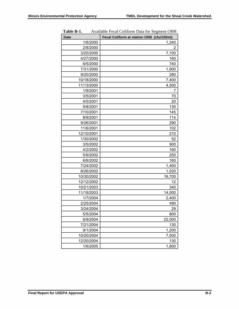
Illinois Environmental Protection Agency TMDL Development for the Shoal Creek Watershed
Final Report for USEPA Approval B-2
Table B-1. Available Fecal Coliform Data for Segment OI08 Date Fecal Coliform at station OI08 (cfu/100ml)
1/6/2000 1,240 2/8/2000 2
3/20/2000 7,100 4/27/2000 160 6/5/2000 740
7/31/2000 1,900 9/20/2000 280
10/18/2000 7,400 11/13/2000 4,500
1/9/2001 7 3/5/2001 70 4/5/2001 20 5/8/2001 130
7/10/2001 145 8/9/2001 114
9/26/2001 290 11/6/2001 102
12/10/2001 210 1/30/2002 52 3/5/2002 900 4/2/2002 160 5/9/2002 250 6/6/2002 160
7/24/2002 1,400 8/26/2002 1,020
10/30/2002 16,700 12/12/2002 12 10/21/2003 340 11/19/2003 14,000
1/7/2004 2,400 2/25/2004 490 3/24/2004 29 5/5/2004 800 6/9/2004 22,000
7/21/2004 130 9/1/2004 1,200
10/20/2004 7,500 12/20/2004 130
1/6/2005 1,800

Illinois Environmental Protection Agency TMDL Development for the Shoal Creek Watershed
Final Report for USEPA Approval B-3
Table B-2. Available Manganese Data for Segment OI08 Date Manganese at Station OI08 (µg/L)
1/21/1999 300 2/10/1999 170 3/24/1999 270 6/1/1999 380 8/3/1999 410
8/26/1999 460 10/7/1999 290 12/1/1999 260 1/6/2000 100 2/8/2000 140
4/27/2000 300 6/5/2000 260
7/31/2000 190 9/20/2000 220
10/18/2000 170 11/13/2000 170
3/5/2001 210 4/5/2001 260 5/8/2001 420
7/10/2001 380 8/9/2001 340
11/6/2001 200 12/10/2001 110
1/30/2002 260 3/5/2002 230 4/2/2002 170 5/9/2002 140 6/6/2002 260
7/24/2002 300 8/26/2002 380
10/30/2002 220 12/12/2002 80
1/15/2003 110 3/12/2003 280 4/16/2003 680 5/14/2003 180 6/17/2003 170 7/30/2003 490 9/10/2003 190
10/21/2003 220 11/19/2003 650
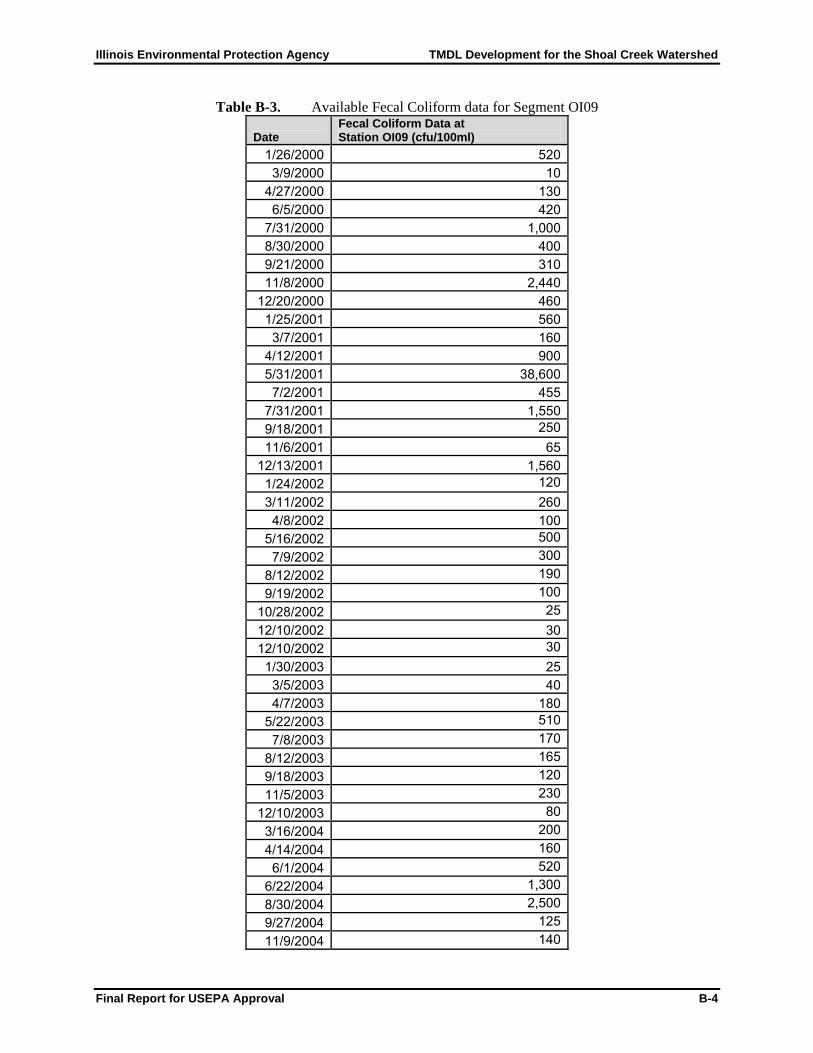
Illinois Environmental Protection Agency TMDL Development for the Shoal Creek Watershed
Final Report for USEPA Approval B-4
Table B-3. Available Fecal Coliform data for Segment OI09
Date Fecal Coliform Data at Station OI09 (cfu/100ml)
1/26/2000 5203/9/2000 10
4/27/2000 1306/5/2000 420
7/31/2000 1,0008/30/2000 4009/21/2000 31011/8/2000 2,440
12/20/2000 4601/25/2001 5603/7/2001 160
4/12/2001 9005/31/2001 38,6007/2/2001 455
7/31/2001 1,5509/18/2001 25011/6/2001 65
12/13/2001 1,5601/24/2002 1203/11/2002 2604/8/2002 100
5/16/2002 5007/9/2002 300
8/12/2002 1909/19/2002 100
10/28/2002 2512/10/2002 3012/10/2002 30
1/30/2003 253/5/2003 404/7/2003 180
5/22/2003 5107/8/2003 170
8/12/2003 1659/18/2003 12011/5/2003 230
12/10/2003 803/16/2004 2004/14/2004 1606/1/2004 520
6/22/2004 1,3008/30/2004 2,5009/27/2004 12511/9/2004 140

Illinois Environmental Protection Agency TMDL Development for the Shoal Creek Watershed
Final Report for USEPA Approval B-5
Date Fecal Coliform Data at Station OI09 (cfu/100ml)
12/29/2004 1205/25/2005 1498/10/2005 9909/26/2005 14,6005/17/2006 2506/26/2006 5458/30/2006 7609/25/2006 120
Table B-4. Available Manganese Data for Segment OI09
Date Manganese at station OI09 (µg/L)
2/3/1999 1403/16/1999 2504/12/1999 1305/25/1999 1507/7/1999 360
8/30/1999 1809/27/1999 7011/3/1999 17012/8/1999 2301/26/2000 2504/27/2000 3707/31/2000 2908/30/2000 1209/21/2000 20011/8/2000 150
12/20/2000 2301/25/2001 1703/7/2001 200
4/12/2001 2805/31/2001 2707/2/2001 270
7/31/2001 31011/6/2001 150
12/13/2001 2603/11/2002 1504/8/2002 220

Illinois Environmental Protection Agency TMDL Development for the Shoal Creek Watershed
Final Report for USEPA Approval B-6
Table B-5. Available Silver Data for Segment OIO09 Date Silver Data at Station OIO09 (µg/L)
4/15/1991 3 10/28/1991 13
Table B-6. Available TDS Data for Segment OIP10 Date TDS at station OIP10 (mg/L)
4/15/1991 3049/18/1991 1,220
10/28/1991 63410/17/2006 928
Table B-7. Available Copper Data for Segment OIP10 Date TDS at station OIP10 (µg/L)
4/15/1991 109/18/1991 1,461
10/28/1991 3410/17/2006 21
Table B-8. Available Ammonia Data for Segment OIP10
Date Ammonia at station OIP10 (mg/L)
4/15/1991 0.389/18/1991 24.00
10/28/1991 3.0010/17/2006 5.80

Illinois Environmental Protection Agency TMDL Development for the Shoal Creek Watershed
Final Report for USEPA Approval C-1
Appendix C : NPDES Fecal Coliform Counts

Illinois Environmental Protection Agency TMDL Development for the Shoal Creek Watershed
Final Report for USEPA Approval C-2
Table C-1. Fecal Coliform Counts from Breese STP (IL0022772)
Date Fecal Count (cfu/100 mL) Average Flow (MGD) Max Flow (MGD) Rec Season 5/31/2005 52 0.392 0.878 Yes 6/30/2005 23 0.36 1.42 Yes 7/31/2005 12 0.429 1.25 Yes 8/31/2005 2 0.369 1.08 Yes 7/31/2006 2 0.541 0.775 Yes
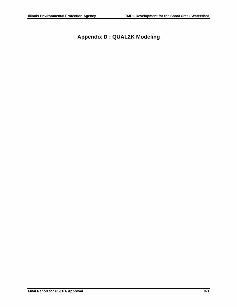
Illinois Environmental Protection Agency TMDL Development for the Shoal Creek Watershed
Final Report for USEPA Approval D-1
Appendix D : QUAL2K Modeling

QUAL2Kw
Stream Water Quality Model
Cattle (10/17/2006)
Headwater and Downstream Boundary Data:
Headwater Flow 0.000 m3/sPrescribed downstream boundary? NoHeadwater Water Quality Units 12:00 AMTemperature C 20.00Conductivity umhos 0.00Inorganic Solids mgD/L 0.00Dissolved Oxygen mg/L 8.00CBODslow mgO2/L 1.00CBODfast mgO2/L 1.00Organic Nitrogen ugN/L 10.00NH4-Nitrogen ugN/L 10.00NO3-Nitrogen ugN/L 0.00Organic Phosphorus ugP/L 0.00Inorganic Phosphorus (SRP) ugP/L 0.00Phytoplankton ugA/L 0.00Detritus (POM) mgD/L 0.00Pathogen cfu/100 mL 0.00Generic constituent user defined 0.00Alkalinity mgCaCO3/L 200.00pH s.u. 7.33
D- 1

QUAL2Kw
Stream Water Quality Model
Cattle (10/17/2006)
Reach Data:
Reach for diel plot: 17Reach Downstream
Reach Downstream length Downstream location Upstream DownstreamLabel end of reach label Number (km) Latitude Longitude (km) (m) (m)
Headwater 0 38.59 89.54 4.250 149.2501 0.25 38.59 89.54 4.000 149.000 147.7502 0.25 38.59 89.54 3.750 147.750 146.5003 0.25 38.59 89.54 3.500 146.500 145.2504 0.25 38.59 89.54 3.250 145.250 144.0005 0.25 38.59 89.54 3.000 144.000 142.7506 0.25 38.59 89.54 2.750 142.750 141.5007 0.25 38.59 89.54 2.500 141.500 140.2508 0.25 38.59 89.54 2.250 140.250 139.0009 0.25 38.59 89.54 2.000 139.000 137.750
10 0.25 38.59 89.54 1.750 137.750 136.50011 0.25 38.59 89.54 1.500 136.500 135.25012 0.25 38.59 89.54 1.250 135.250 134.00013 0.25 38.59 89.54 1.000 134.000 133.00014 0.25 38.59 89.54 0.750 133.000 132.00015 0.25 38.59 89.54 0.500 132.000 131.00016 0.25 38.59 89.54 0.250 131.000 130.00017 0.25 38.59 89.54 0.000 130.000 129.000
Elevation
D- 2

Number0123456789
1011121314151617
QUAL2Kw
Stream Water Quality Model
Cattle (10/17/2006)
Reach Data:
Hydraulic Model (Weir Overrides Rating Curves; Rating Curve Rating Curves
Height WidthDegrees Minutes Seconds Degrees Minutes Seconds (m) (m) Coefficient Exponent Coefficient Exponent
38.00 35 0 89.00 32 0 0.0000 0.0000 0.0000 0.000 0.0000 0.00038.00 35 0 89.00 32 0 0.0000 0.0000 0.0000 0.000 0.0000 0.00038.00 35 0 89.00 32 0 0.0000 0.0000 0.0000 0.000 0.0000 0.00038.00 35 0 89.00 32 0 0.0000 0.0000 0.0000 0.000 0.0000 0.00038.00 35 0 89.00 32 0 0.0000 0.0000 0.0000 0.000 0.0000 0.00038.00 35 0 89.00 32 0 0.0000 0.0000 0.0000 0.000 0.0000 0.00038.00 35 0 89.00 32 0 0.0000 0.0000 0.0000 0.000 0.0000 0.00038.00 35 0 89.00 32 0 0.0000 0.0000 0.0000 0.000 0.0000 0.00038.00 35 0 89.00 32 0 0.0000 0.0000 0.0000 0.000 0.0000 0.00038.00 35 0 89.00 32 0 0.0000 0.0000 0.0000 0.000 0.0000 0.00038.00 35 0 89.00 32 0 0.0000 0.0000 0.0000 0.000 0.0000 0.00038.00 35 0 89.00 32 0 0.0000 0.0000 0.0000 0.000 0.0000 0.00038.00 35 0 89.00 32 0 0.0000 0.0000 0.0000 0.000 0.0000 0.00038.00 35 0 89.00 32 0 0.0000 0.0000 0.0000 0.000 0.0000 0.00038.00 35 0 89.00 32 0 0.0000 0.0000 0.0000 0.000 0.0000 0.00038.00 35 0 89.00 32 0 0.0000 0.0000 0.0000 0.000 0.0000 0.00038.00 35 0 89.00 32 0 0.0000 0.0000 0.0000 0.000 0.0000 0.00038.00 35 0 89.00 32 0 0.0000 0.0000 0.0000 0.000 0.0000 0.000
Velocity DepthDownstream Weir
Latitude Longitude
D- 3

Number0123456789
1011121314151617
QUAL2Kw
Stream Water Quality Model
Cattle (10/17/2006)
Reach Data:
es Override Manning Formula) Manning Formula Prescribed Bottom Bottom Prescribed Prescribed Prescribed
Channel Manning Bot Width Side Side Dispersion Algae SOD SOD CH4 flux NH4 fluxSlope n m Slope Slope m2/s Coverage Coverage gO2/m2/d gO2/m2/d mgN/m2/d0.000050 0.0550 0.37 2.00 2.00 0.000.000050 0.0550 0.37 2.00 2.00 0.00 0% 100% 3.00 0.0000 0.00000.000050 0.0550 0.37 2.00 2.00 0.00 0% 100% 3.00 0.0000 0.00000.000050 0.0550 0.37 2.00 2.00 0.00 0% 100% 3.00 0.0000 0.00000.000050 0.0550 0.37 2.00 2.00 0.00 0% 100% 3.00 0.0000 0.00000.000050 0.0550 0.37 2.00 2.00 0.00 0% 100% 3.00 0.0000 0.00000.000050 0.0550 0.37 2.00 2.00 0.00 0% 100% 3.00 0.0000 0.00000.000050 0.0550 0.37 2.00 2.00 0.00 0% 100% 3.00 0.0000 0.00000.000050 0.0550 0.37 2.00 2.00 0.00 0% 100% 3.00 0.0000 0.00000.000050 0.0550 0.37 2.00 2.00 0.00 0% 100% 3.00 0.0000 0.00000.000050 0.0550 0.37 2.00 2.00 0.00 0% 100% 3.00 0.0000 0.00000.000050 0.0550 0.37 2.00 2.00 0.00 0% 100% 3.00 0.0000 0.00000.000050 0.0550 0.37 2.00 2.00 0.00 0% 100% 3.00 0.0000 0.00000.000050 0.0550 0.37 2.00 2.00 0.00 0% 100% 3.00 0.0000 0.00000.000050 0.0550 0.37 2.00 2.00 0.00 0% 100% 3.00 0.0000 0.00000.000050 0.0550 0.37 2.00 2.00 0.00 0% 100% 3.00 0.0000 0.00000.000050 0.0550 0.37 2.00 2.00 0.00 0% 100% 3.00 0.0000 0.00000.000050 0.0550 0.37 2.00 2.00 0.00 0% 100% 3.00 0.0000 0.0000
D- 4

Number0123456789
1011121314151617
QUAL2Kw
Stream Water Quality Model
Cattle (10/17/2006)
Reach Data:
Prescribed Sediment Sediment Sediment/hyporheic Hyporheic HyporheicInorg P flux thermal cond thermal diff zone thickness exchange flow sediment porositymgP/m2/d (W/m/degC) (cm^2/sec) (cm) (fraction of stream flow) (fraction of volume)
0.0000 1.6 0.0064 10 5% 40%0.0000 1.6 0.0064 10 5% 40%0.0000 1.6 0.0064 10 5% 40%0.0000 1.6 0.0064 10 5% 40%0.0000 1.6 0.0064 10 5% 40%0.0000 1.6 0.0064 10 5% 40%0.0000 1.6 0.0064 10 5% 40%0.0000 1.6 0.0064 10 5% 40%0.0000 1.6 0.0064 10 5% 40%0.0000 1.6 0.0064 10 5% 40%0.0000 1.6 0.0064 10 5% 40%0.0000 1.6 0.0064 10 5% 40%0.0000 1.6 0.0064 10 5% 40%0.0000 1.6 0.0064 10 5% 40%0.0000 1.6 0.0064 10 5% 40%0.0000 1.6 0.0064 10 5% 40%0.0000 1.6 0.0064 10 5% 40%
D- 5

QUAL2Kw
Stream Water Quality Model
Cattle (10/17/2006)
Air Temperature Data:
Upstream Downstream 12:00 AM 1:00 AM 2:00 AM 3:00 AM 4:00 AMUpstream Reach Downstream Reach Distance Distance Hourly air temperature for each reach (degrees C)
Label Label Label Number km kmHeadwater 1 4.25 4.00 13.00 14.00 16.00 16.00 14.00
2 4.00 3.75 13.00 14.00 16.00 16.00 14.003 3.75 3.50 13.00 14.00 16.00 16.00 14.004 3.50 3.25 13.00 14.00 16.00 16.00 14.005 3.25 3.00 13.00 14.00 16.00 16.00 14.006 3.00 2.75 13.00 14.00 16.00 16.00 14.007 2.75 2.50 13.00 14.00 16.00 16.00 14.008 2.50 2.25 13.00 14.00 16.00 16.00 14.009 2.25 2.00 13.00 14.00 16.00 16.00 14.00
10 2.00 1.75 13.00 14.00 16.00 16.00 14.0011 1.75 1.50 13.00 14.00 16.00 16.00 14.0012 1.50 1.25 13.00 14.00 16.00 16.00 14.0013 1.25 1.00 13.00 14.00 16.00 16.00 14.0014 1.00 0.75 13.00 14.00 16.00 16.00 14.0015 0.75 0.50 13.00 14.00 16.00 16.00 14.0016 0.50 0.25 13.00 14.00 16.00 16.00 14.0017 0.25 0.00 13.00 14.00 16.00 16.00 14.00
(The input values are applied as point estimates at each time. Linear interpolation is used to estimate values between the hourly inputs.)
D- 6

Reach
Number123456789
1011121314151617
QUAL2Kw
Stream Water Quality Model
Cattle (10/17/2006)
Air Temperature Data:
5:00 AM 6:00 AM 7:00 AM 8:00 AM 9:00 AM 10:00 AM 11:00 AM 12:00 PM 1:00 PM 2:00 PM
13.00 13.00 13.00 13.00 13.00 14.00 14.00 15.00 16.00 16.0013.00 13.00 13.00 13.00 13.00 14.00 14.00 15.00 16.00 16.0013.00 13.00 13.00 13.00 13.00 14.00 14.00 15.00 16.00 16.0013.00 13.00 13.00 13.00 13.00 14.00 14.00 15.00 16.00 16.0013.00 13.00 13.00 13.00 13.00 14.00 14.00 15.00 16.00 16.0013.00 13.00 13.00 13.00 13.00 14.00 14.00 15.00 16.00 16.0013.00 13.00 13.00 13.00 13.00 14.00 14.00 15.00 16.00 16.0013.00 13.00 13.00 13.00 13.00 14.00 14.00 15.00 16.00 16.0013.00 13.00 13.00 13.00 13.00 14.00 14.00 15.00 16.00 16.0013.00 13.00 13.00 13.00 13.00 14.00 14.00 15.00 16.00 16.0013.00 13.00 13.00 13.00 13.00 14.00 14.00 15.00 16.00 16.0013.00 13.00 13.00 13.00 13.00 14.00 14.00 15.00 16.00 16.0013.00 13.00 13.00 13.00 13.00 14.00 14.00 15.00 16.00 16.0013.00 13.00 13.00 13.00 13.00 14.00 14.00 15.00 16.00 16.0013.00 13.00 13.00 13.00 13.00 14.00 14.00 15.00 16.00 16.0013.00 13.00 13.00 13.00 13.00 14.00 14.00 15.00 16.00 16.0013.00 13.00 13.00 13.00 13.00 14.00 14.00 15.00 16.00 16.00
D- 7

Reach
Number123456789
1011121314151617
QUAL2Kw
Stream Water Quality Model
Cattle (10/17/2006)
Air Temperature Data:
3:00 PM 4:00 PM 5:00 PM 6:00 PM 7:00 PM 8:00 PM 9:00 PM 10:00 PM 11:00 PM
16.00 16.00 15.00 15.00 15.00 14.00 15.00 14.00 14.0016.00 16.00 15.00 15.00 15.00 14.00 15.00 14.00 14.0016.00 16.00 15.00 15.00 15.00 14.00 15.00 14.00 14.0016.00 16.00 15.00 15.00 15.00 14.00 15.00 14.00 14.0016.00 16.00 15.00 15.00 15.00 14.00 15.00 14.00 14.0016.00 16.00 15.00 15.00 15.00 14.00 15.00 14.00 14.0016.00 16.00 15.00 15.00 15.00 14.00 15.00 14.00 14.0016.00 16.00 15.00 15.00 15.00 14.00 15.00 14.00 14.0016.00 16.00 15.00 15.00 15.00 14.00 15.00 14.00 14.0016.00 16.00 15.00 15.00 15.00 14.00 15.00 14.00 14.0016.00 16.00 15.00 15.00 15.00 14.00 15.00 14.00 14.0016.00 16.00 15.00 15.00 15.00 14.00 15.00 14.00 14.0016.00 16.00 15.00 15.00 15.00 14.00 15.00 14.00 14.0016.00 16.00 15.00 15.00 15.00 14.00 15.00 14.00 14.0016.00 16.00 15.00 15.00 15.00 14.00 15.00 14.00 14.0016.00 16.00 15.00 15.00 15.00 14.00 15.00 14.00 14.0016.00 16.00 15.00 15.00 15.00 14.00 15.00 14.00 14.00
D- 8

QUAL2Kw
Stream Water Quality Model
Cattle (10/17/2006)
Dew Point Temperature Data:
Upstream Downstream 12:00 AM 1:00 AM 2:00 AM 3:00 AM 4:00 AMUpstream Reach Downstream Reach Distance Distance Hourly dewpoint temperature for each reach (degrees C)
Label Label Label Number km kmHeadwater 1 4.25 4.00 12.00 13.00 15.00 14.00 12.00
2 4.00 3.75 12.00 13.00 15.00 14.00 12.003 3.75 3.50 12.00 13.00 15.00 14.00 12.004 3.50 3.25 12.00 13.00 15.00 14.00 12.005 3.25 3.00 12.00 13.00 15.00 14.00 12.006 3.00 2.75 12.00 13.00 15.00 14.00 12.007 2.75 2.50 12.00 13.00 15.00 14.00 12.008 2.50 2.25 12.00 13.00 15.00 14.00 12.009 2.25 2.00 12.00 13.00 15.00 14.00 12.00
10 2.00 1.75 12.00 13.00 15.00 14.00 12.0011 1.75 1.50 12.00 13.00 15.00 14.00 12.0012 1.50 1.25 12.00 13.00 15.00 14.00 12.0013 1.25 1.00 12.00 13.00 15.00 14.00 12.0014 1.00 0.75 12.00 13.00 15.00 14.00 12.0015 0.75 0.50 12.00 13.00 15.00 14.00 12.0016 0.50 0.25 12.00 13.00 15.00 14.00 12.0017 0.25 0.00 12.00 13.00 15.00 14.00 12.00
(The input values are applied as point estimates at each time. Linear interpolation is used to estimate values between the hourly inputs.)
D- 9

Reach
Number123456789
1011121314151617
QUAL2Kw
Stream Water Quality Model
Cattle (10/17/2006)
Dew Point Temperature Data:
5:00 AM 6:00 AM 7:00 AM 8:00 AM 9:00 AM 10:00 AM 11:00 AM 12:00 PM 1:00 PM 2:00 PM
11.00 11.00 11.00 11.00 11.00 12.00 12.00 12.00 12.00 13.0011.00 11.00 11.00 11.00 11.00 12.00 12.00 12.00 12.00 13.0011.00 11.00 11.00 11.00 11.00 12.00 12.00 12.00 12.00 13.0011.00 11.00 11.00 11.00 11.00 12.00 12.00 12.00 12.00 13.0011.00 11.00 11.00 11.00 11.00 12.00 12.00 12.00 12.00 13.0011.00 11.00 11.00 11.00 11.00 12.00 12.00 12.00 12.00 13.0011.00 11.00 11.00 11.00 11.00 12.00 12.00 12.00 12.00 13.0011.00 11.00 11.00 11.00 11.00 12.00 12.00 12.00 12.00 13.0011.00 11.00 11.00 11.00 11.00 12.00 12.00 12.00 12.00 13.0011.00 11.00 11.00 11.00 11.00 12.00 12.00 12.00 12.00 13.0011.00 11.00 11.00 11.00 11.00 12.00 12.00 12.00 12.00 13.0011.00 11.00 11.00 11.00 11.00 12.00 12.00 12.00 12.00 13.0011.00 11.00 11.00 11.00 11.00 12.00 12.00 12.00 12.00 13.0011.00 11.00 11.00 11.00 11.00 12.00 12.00 12.00 12.00 13.0011.00 11.00 11.00 11.00 11.00 12.00 12.00 12.00 12.00 13.0011.00 11.00 11.00 11.00 11.00 12.00 12.00 12.00 12.00 13.0011.00 11.00 11.00 11.00 11.00 12.00 12.00 12.00 12.00 13.00
D-10

Reach
Number123456789
1011121314151617
QUAL2Kw
Stream Water Quality Model
Cattle (10/17/2006)
Dew Point Temperature Data:
3:00 PM 4:00 PM 5:00 PM 6:00 PM 7:00 PM 8:00 PM 9:00 PM 10:00 PM 11:00 PM
13.00 13.00 13.00 13.00 13.00 13.00 13.00 13.00 13.0013.00 13.00 13.00 13.00 13.00 13.00 13.00 13.00 13.0013.00 13.00 13.00 13.00 13.00 13.00 13.00 13.00 13.0013.00 13.00 13.00 13.00 13.00 13.00 13.00 13.00 13.0013.00 13.00 13.00 13.00 13.00 13.00 13.00 13.00 13.0013.00 13.00 13.00 13.00 13.00 13.00 13.00 13.00 13.0013.00 13.00 13.00 13.00 13.00 13.00 13.00 13.00 13.0013.00 13.00 13.00 13.00 13.00 13.00 13.00 13.00 13.0013.00 13.00 13.00 13.00 13.00 13.00 13.00 13.00 13.0013.00 13.00 13.00 13.00 13.00 13.00 13.00 13.00 13.0013.00 13.00 13.00 13.00 13.00 13.00 13.00 13.00 13.0013.00 13.00 13.00 13.00 13.00 13.00 13.00 13.00 13.0013.00 13.00 13.00 13.00 13.00 13.00 13.00 13.00 13.0013.00 13.00 13.00 13.00 13.00 13.00 13.00 13.00 13.0013.00 13.00 13.00 13.00 13.00 13.00 13.00 13.00 13.0013.00 13.00 13.00 13.00 13.00 13.00 13.00 13.00 13.0013.00 13.00 13.00 13.00 13.00 13.00 13.00 13.00 13.00
D-11

QUAL2Kw
Stream Water Quality Model
Cattle (10/17/2006)
Wind Speed Data:
Upstream Downstream 12:00 AM 1:00 AM 2:00 AM 3:00 AM 4:00 AMUpstream Reach Downstream Reach Distance Distance Wind speed for each reach 7m above water surface (m/s)
Label Label Label Number km kmHeadwater 1 4.25 4.00 4.02 4.02 3.58 7.15 8.94
2 4.00 3.75 4.02 4.02 3.58 7.15 8.943 3.75 3.50 4.02 4.02 3.58 7.15 8.944 3.50 3.25 4.02 4.02 3.58 7.15 8.945 3.25 3.00 4.02 4.02 3.58 7.15 8.946 3.00 2.75 4.02 4.02 3.58 7.15 8.947 2.75 2.50 4.02 4.02 3.58 7.15 8.948 2.50 2.25 4.02 4.02 3.58 7.15 8.949 2.25 2.00 4.02 4.02 3.58 7.15 8.94
10 2.00 1.75 4.02 4.02 3.58 7.15 8.9411 1.75 1.50 4.02 4.02 3.58 7.15 8.9412 1.50 1.25 4.02 4.02 3.58 7.15 8.9413 1.25 1.00 4.02 4.02 3.58 7.15 8.9414 1.00 0.75 4.02 4.02 3.58 7.15 8.9415 0.75 0.50 4.02 4.02 3.58 7.15 8.9416 0.50 0.25 4.02 4.02 3.58 7.15 8.9417 0.25 0.00 4.02 4.02 3.58 7.15 8.94
(The input values are applied as point estimates at each time. Linear interpolation is used to estimate values between the hourly inputs.)
D-12
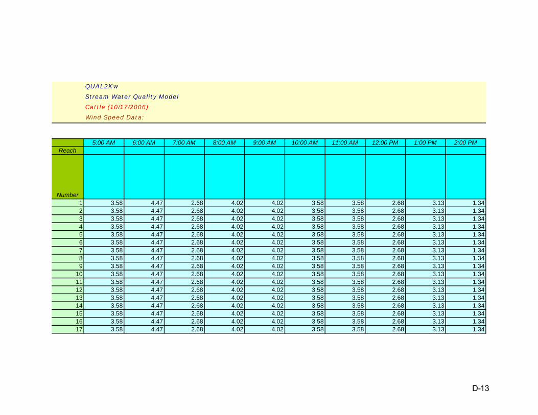
Reach
Number123456789
1011121314151617
QUAL2Kw
Stream Water Quality Model
Cattle (10/17/2006)
Wind Speed Data:
5:00 AM 6:00 AM 7:00 AM 8:00 AM 9:00 AM 10:00 AM 11:00 AM 12:00 PM 1:00 PM 2:00 PM
3.58 4.47 2.68 4.02 4.02 3.58 3.58 2.68 3.13 1.343.58 4.47 2.68 4.02 4.02 3.58 3.58 2.68 3.13 1.343.58 4.47 2.68 4.02 4.02 3.58 3.58 2.68 3.13 1.343.58 4.47 2.68 4.02 4.02 3.58 3.58 2.68 3.13 1.343.58 4.47 2.68 4.02 4.02 3.58 3.58 2.68 3.13 1.343.58 4.47 2.68 4.02 4.02 3.58 3.58 2.68 3.13 1.343.58 4.47 2.68 4.02 4.02 3.58 3.58 2.68 3.13 1.343.58 4.47 2.68 4.02 4.02 3.58 3.58 2.68 3.13 1.343.58 4.47 2.68 4.02 4.02 3.58 3.58 2.68 3.13 1.343.58 4.47 2.68 4.02 4.02 3.58 3.58 2.68 3.13 1.343.58 4.47 2.68 4.02 4.02 3.58 3.58 2.68 3.13 1.343.58 4.47 2.68 4.02 4.02 3.58 3.58 2.68 3.13 1.343.58 4.47 2.68 4.02 4.02 3.58 3.58 2.68 3.13 1.343.58 4.47 2.68 4.02 4.02 3.58 3.58 2.68 3.13 1.343.58 4.47 2.68 4.02 4.02 3.58 3.58 2.68 3.13 1.343.58 4.47 2.68 4.02 4.02 3.58 3.58 2.68 3.13 1.343.58 4.47 2.68 4.02 4.02 3.58 3.58 2.68 3.13 1.34
D-13
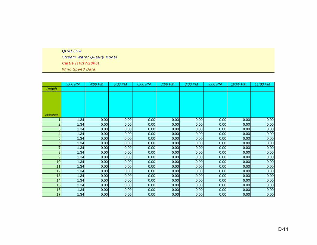
Reach
Number123456789
1011121314151617
QUAL2Kw
Stream Water Quality Model
Cattle (10/17/2006)
Wind Speed Data:
3:00 PM 4:00 PM 5:00 PM 6:00 PM 7:00 PM 8:00 PM 9:00 PM 10:00 PM 11:00 PM
1.34 0.00 0.00 0.00 0.00 0.00 0.00 0.00 0.001.34 0.00 0.00 0.00 0.00 0.00 0.00 0.00 0.001.34 0.00 0.00 0.00 0.00 0.00 0.00 0.00 0.001.34 0.00 0.00 0.00 0.00 0.00 0.00 0.00 0.001.34 0.00 0.00 0.00 0.00 0.00 0.00 0.00 0.001.34 0.00 0.00 0.00 0.00 0.00 0.00 0.00 0.001.34 0.00 0.00 0.00 0.00 0.00 0.00 0.00 0.001.34 0.00 0.00 0.00 0.00 0.00 0.00 0.00 0.001.34 0.00 0.00 0.00 0.00 0.00 0.00 0.00 0.001.34 0.00 0.00 0.00 0.00 0.00 0.00 0.00 0.001.34 0.00 0.00 0.00 0.00 0.00 0.00 0.00 0.001.34 0.00 0.00 0.00 0.00 0.00 0.00 0.00 0.001.34 0.00 0.00 0.00 0.00 0.00 0.00 0.00 0.001.34 0.00 0.00 0.00 0.00 0.00 0.00 0.00 0.001.34 0.00 0.00 0.00 0.00 0.00 0.00 0.00 0.001.34 0.00 0.00 0.00 0.00 0.00 0.00 0.00 0.001.34 0.00 0.00 0.00 0.00 0.00 0.00 0.00 0.00
D-14

QUAL2Kw
Stream Water Quality Model
Cattle (10/17/2006)
Cloud Cover Data:
Upstream Downstream 12:00 AM 1:00 AM 2:00 AM 3:00 AM 4:00 AMUpstream Reach Downstream Reach Distance Distance Hourly cloud cover shade for each reach (Percent)
Label Label Label Number km kmHeadwater 1 4.25 4.00 95.0% 95.0% 95.0% 95.0% 95.0%
2 4.00 3.75 95.0% 95.0% 95.0% 95.0% 95.0%3 3.75 3.50 95.0% 95.0% 95.0% 95.0% 95.0%4 3.50 3.25 95.0% 95.0% 95.0% 95.0% 95.0%5 3.25 3.00 95.0% 95.0% 95.0% 95.0% 95.0%6 3.00 2.75 95.0% 95.0% 95.0% 95.0% 95.0%7 2.75 2.50 95.0% 95.0% 95.0% 95.0% 95.0%8 2.50 2.25 95.0% 95.0% 95.0% 95.0% 95.0%9 2.25 2.00 95.0% 95.0% 95.0% 95.0% 95.0%
10 2.00 1.75 95.0% 95.0% 95.0% 95.0% 95.0%11 1.75 1.50 95.0% 95.0% 95.0% 95.0% 95.0%12 1.50 1.25 95.0% 95.0% 95.0% 95.0% 95.0%13 1.25 1.00 95.0% 95.0% 95.0% 95.0% 95.0%14 1.00 0.75 95.0% 95.0% 95.0% 95.0% 95.0%15 0.75 0.50 95.0% 95.0% 95.0% 95.0% 95.0%16 0.50 0.25 95.0% 95.0% 95.0% 95.0% 95.0%17 0.25 0.00 95.0% 95.0% 95.0% 95.0% 95.0%
(Percent of sky that is covered by clouds. The input values are applied as point estimates at each time. Linear interpolation is used to estimate values between the hourly inputs.)
D-15

Reach
Number123456789
1011121314151617
QUAL2Kw
Stream Water Quality Model
Cattle (10/17/2006)
Cloud Cover Data:
5:00 AM 6:00 AM 7:00 AM 8:00 AM 9:00 AM 10:00 AM 11:00 AM 12:00 PM 1:00 PM 2:00 PM
72.5% 95.0% 95.0% 95.0% 95.0% 95.0% 95.0% 91.3% 95.0% 95.0%72.5% 95.0% 95.0% 95.0% 95.0% 95.0% 95.0% 91.3% 95.0% 95.0%72.5% 95.0% 95.0% 95.0% 95.0% 95.0% 95.0% 91.3% 95.0% 95.0%72.5% 95.0% 95.0% 95.0% 95.0% 95.0% 95.0% 91.3% 95.0% 95.0%72.5% 95.0% 95.0% 95.0% 95.0% 95.0% 95.0% 91.3% 95.0% 95.0%72.5% 95.0% 95.0% 95.0% 95.0% 95.0% 95.0% 91.3% 95.0% 95.0%72.5% 95.0% 95.0% 95.0% 95.0% 95.0% 95.0% 91.3% 95.0% 95.0%72.5% 95.0% 95.0% 95.0% 95.0% 95.0% 95.0% 91.3% 95.0% 95.0%72.5% 95.0% 95.0% 95.0% 95.0% 95.0% 95.0% 91.3% 95.0% 95.0%72.5% 95.0% 95.0% 95.0% 95.0% 95.0% 95.0% 91.3% 95.0% 95.0%72.5% 95.0% 95.0% 95.0% 95.0% 95.0% 95.0% 91.3% 95.0% 95.0%72.5% 95.0% 95.0% 95.0% 95.0% 95.0% 95.0% 91.3% 95.0% 95.0%72.5% 95.0% 95.0% 95.0% 95.0% 95.0% 95.0% 91.3% 95.0% 95.0%72.5% 95.0% 95.0% 95.0% 95.0% 95.0% 95.0% 91.3% 95.0% 95.0%72.5% 95.0% 95.0% 95.0% 95.0% 95.0% 95.0% 91.3% 95.0% 95.0%72.5% 95.0% 95.0% 95.0% 95.0% 95.0% 95.0% 91.3% 95.0% 95.0%72.5% 95.0% 95.0% 95.0% 95.0% 95.0% 95.0% 91.3% 95.0% 95.0%
D-16

Reach
Number123456789
1011121314151617
QUAL2Kw
Stream Water Quality Model
Cattle (10/17/2006)
Cloud Cover Data:
3:00 PM 4:00 PM 5:00 PM 6:00 PM 7:00 PM 8:00 PM 9:00 PM 10:00 PM 11:00 PM
95.0% 95.0% 95.0% 95.0% 95.0% 95.0% 95.0% 95.0% 95.0%95.0% 95.0% 95.0% 95.0% 95.0% 95.0% 95.0% 95.0% 95.0%95.0% 95.0% 95.0% 95.0% 95.0% 95.0% 95.0% 95.0% 95.0%95.0% 95.0% 95.0% 95.0% 95.0% 95.0% 95.0% 95.0% 95.0%95.0% 95.0% 95.0% 95.0% 95.0% 95.0% 95.0% 95.0% 95.0%95.0% 95.0% 95.0% 95.0% 95.0% 95.0% 95.0% 95.0% 95.0%95.0% 95.0% 95.0% 95.0% 95.0% 95.0% 95.0% 95.0% 95.0%95.0% 95.0% 95.0% 95.0% 95.0% 95.0% 95.0% 95.0% 95.0%95.0% 95.0% 95.0% 95.0% 95.0% 95.0% 95.0% 95.0% 95.0%95.0% 95.0% 95.0% 95.0% 95.0% 95.0% 95.0% 95.0% 95.0%95.0% 95.0% 95.0% 95.0% 95.0% 95.0% 95.0% 95.0% 95.0%95.0% 95.0% 95.0% 95.0% 95.0% 95.0% 95.0% 95.0% 95.0%95.0% 95.0% 95.0% 95.0% 95.0% 95.0% 95.0% 95.0% 95.0%95.0% 95.0% 95.0% 95.0% 95.0% 95.0% 95.0% 95.0% 95.0%95.0% 95.0% 95.0% 95.0% 95.0% 95.0% 95.0% 95.0% 95.0%95.0% 95.0% 95.0% 95.0% 95.0% 95.0% 95.0% 95.0% 95.0%95.0% 95.0% 95.0% 95.0% 95.0% 95.0% 95.0% 95.0% 95.0%
D-17

QUAL2Kw
Stream Water Quality Model
Cattle (10/17/2006)
Shade Data:
Upstream Downstream 12:00 AM 1:00 AM 2:00 AM 3:00 AM 4:00 AMUpstream Reach Downstream Reach Distance Distance Integrated hourly effective shade for each reach (Percent)
Label Label Label Number km kmHeadwater 1 4.25 4.00 15.0% 15.0% 15.0% 15.0% 15.0%
2 4.00 3.75 15.0% 15.0% 15.0% 15.0% 15.0%3 3.75 3.50 15.0% 15.0% 15.0% 15.0% 15.0%4 3.50 3.25 15.0% 15.0% 15.0% 15.0% 15.0%5 3.25 3.00 15.0% 15.0% 15.0% 15.0% 15.0%6 3.00 2.75 15.0% 15.0% 15.0% 15.0% 15.0%7 2.75 2.50 15.0% 15.0% 15.0% 15.0% 15.0%8 2.50 2.25 15.0% 15.0% 15.0% 15.0% 15.0%9 2.25 2.00 15.0% 15.0% 15.0% 15.0% 15.0%
10 2.00 1.75 15.0% 15.0% 15.0% 15.0% 15.0%11 1.75 1.50 15.0% 15.0% 15.0% 15.0% 15.0%12 1.50 1.25 15.0% 15.0% 15.0% 15.0% 15.0%13 1.25 1.00 15.0% 15.0% 15.0% 15.0% 15.0%14 1.00 0.75 15.0% 15.0% 15.0% 15.0% 15.0%15 0.75 0.50 15.0% 15.0% 15.0% 15.0% 15.0%16 0.50 0.25 15.0% 15.0% 15.0% 15.0% 15.0%17 0.25 0.00 15.0% 15.0% 15.0% 15.0% 15.0%
(Percent of solar radiation that is blocked because of shade from topography and vegetation. Hourly values are applied as integrated values for each hour, e.g. the value at 12:00 AM is applied from 12:00 to 1:00 AM)
D-18

Reach
Number123456789
1011121314151617
QUAL2Kw
Stream Water Quality Model
Cattle (10/17/2006)
Shade Data:
5:00 AM 6:00 AM 7:00 AM 8:00 AM 9:00 AM 10:00 AM 11:00 AM 12:00 PM 1:00 PM 2:00 PM
15.0% 15.0% 15.0% 15.0% 15.0% 15.0% 15.0% 15.0% 15.0% 15.0%15.0% 15.0% 15.0% 15.0% 15.0% 15.0% 15.0% 15.0% 15.0% 15.0%15.0% 15.0% 15.0% 15.0% 15.0% 15.0% 15.0% 15.0% 15.0% 15.0%15.0% 15.0% 15.0% 15.0% 15.0% 15.0% 15.0% 15.0% 15.0% 15.0%15.0% 15.0% 15.0% 15.0% 15.0% 15.0% 15.0% 15.0% 15.0% 15.0%15.0% 15.0% 15.0% 15.0% 15.0% 15.0% 15.0% 15.0% 15.0% 15.0%15.0% 15.0% 15.0% 15.0% 15.0% 15.0% 15.0% 15.0% 15.0% 15.0%15.0% 15.0% 15.0% 15.0% 15.0% 15.0% 15.0% 15.0% 15.0% 15.0%15.0% 15.0% 15.0% 15.0% 15.0% 15.0% 15.0% 15.0% 15.0% 15.0%15.0% 15.0% 15.0% 15.0% 15.0% 15.0% 15.0% 15.0% 15.0% 15.0%15.0% 15.0% 15.0% 15.0% 15.0% 15.0% 15.0% 15.0% 15.0% 15.0%15.0% 15.0% 15.0% 15.0% 15.0% 15.0% 15.0% 15.0% 15.0% 15.0%15.0% 15.0% 15.0% 15.0% 15.0% 15.0% 15.0% 15.0% 15.0% 15.0%15.0% 15.0% 15.0% 15.0% 15.0% 15.0% 15.0% 15.0% 15.0% 15.0%15.0% 15.0% 15.0% 15.0% 15.0% 15.0% 15.0% 15.0% 15.0% 15.0%15.0% 15.0% 15.0% 15.0% 15.0% 15.0% 15.0% 15.0% 15.0% 15.0%15.0% 15.0% 15.0% 15.0% 15.0% 15.0% 15.0% 15.0% 15.0% 15.0%
D-19
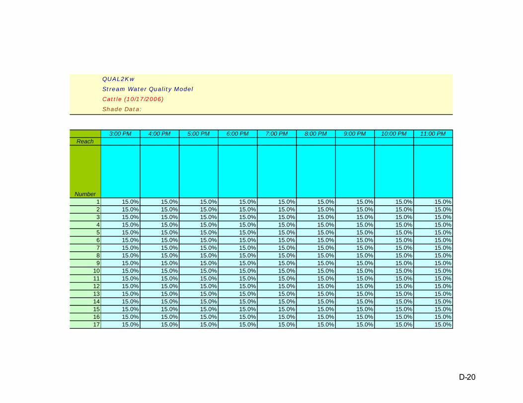
Reach
Number123456789
1011121314151617
QUAL2Kw
Stream Water Quality Model
Cattle (10/17/2006)
Shade Data:
3:00 PM 4:00 PM 5:00 PM 6:00 PM 7:00 PM 8:00 PM 9:00 PM 10:00 PM 11:00 PM
15.0% 15.0% 15.0% 15.0% 15.0% 15.0% 15.0% 15.0% 15.0%15.0% 15.0% 15.0% 15.0% 15.0% 15.0% 15.0% 15.0% 15.0%15.0% 15.0% 15.0% 15.0% 15.0% 15.0% 15.0% 15.0% 15.0%15.0% 15.0% 15.0% 15.0% 15.0% 15.0% 15.0% 15.0% 15.0%15.0% 15.0% 15.0% 15.0% 15.0% 15.0% 15.0% 15.0% 15.0%15.0% 15.0% 15.0% 15.0% 15.0% 15.0% 15.0% 15.0% 15.0%15.0% 15.0% 15.0% 15.0% 15.0% 15.0% 15.0% 15.0% 15.0%15.0% 15.0% 15.0% 15.0% 15.0% 15.0% 15.0% 15.0% 15.0%15.0% 15.0% 15.0% 15.0% 15.0% 15.0% 15.0% 15.0% 15.0%15.0% 15.0% 15.0% 15.0% 15.0% 15.0% 15.0% 15.0% 15.0%15.0% 15.0% 15.0% 15.0% 15.0% 15.0% 15.0% 15.0% 15.0%15.0% 15.0% 15.0% 15.0% 15.0% 15.0% 15.0% 15.0% 15.0%15.0% 15.0% 15.0% 15.0% 15.0% 15.0% 15.0% 15.0% 15.0%15.0% 15.0% 15.0% 15.0% 15.0% 15.0% 15.0% 15.0% 15.0%15.0% 15.0% 15.0% 15.0% 15.0% 15.0% 15.0% 15.0% 15.0%15.0% 15.0% 15.0% 15.0% 15.0% 15.0% 15.0% 15.0% 15.0%15.0% 15.0% 15.0% 15.0% 15.0% 15.0% 15.0% 15.0% 15.0%
D-20

QUAL2Kw
Stream Water Quality Model
Cattle (10/17/2006)
Light Parameters and Surface Heat Transfer Models:
Parameter Value UnitPhotosynthetically Available Radiation 0.47Background light extinction 0.2 /m k eb
Linear chlorophyll light extinction 0.0088 1/m-(ugA/L) α p
Nonlinear chlorophyll light extinction 0.054 1/m-(ugA/L) 2/3 α pn
ISS light extinction 0.052 1/m-(mgD/L) α ι
Detritus light extinction 0.174 1/m-(mgD/L) α ο
Macrophyte light extinction 0.015 1/m-(gD/m 3 ) α mac
Solar shortwave radiation modelAtmospheric attenuation model for solar Ryan-StolzenbachBras solar parameter (used if Bras solar model is selected)atmospheric turbidity coefficient (2=clear, 5=smoggy, default=2) 2 n fac
Ryan-Stolzenbach solar parameter (used if Ryan-Stolzenbach solar model is selected)atmospheric transmission coefficient (0.70-0.91, default 0.8) 0.8 a tc
Downwelling atmospheric longwave IR radiationatmospheric longwave emissivity model BruntEvaporation and air convection/conductionwind speed function for evaporation and air convection/conduction Brady-Graves-Geyer
D-21

QUAL2Kw
Stream Water Quality Model
Cattle (10/17/2006)
Diffuse Source Data:
Diffuse Diffuse Spec Inorg Diss CBOD CBODAbstraction Inflow Temp Cond SS Oxygen slow fast
Name Up (km) Down (km) m3/s m3/s C umhos mgD/L mg/L mgO2/L mgO2/L1.00 4.2500 1.0000 0.00 0.0007 27.00 0.00 0.00 3.50 300.0 250.01.00 1.0000 0.0000 0.0001 27.00 0.00 0.00 3.50 300.0 250.0
D-22

Organic Ammon Nitrate Organic Inorganic Phyto GenericN N N P P plankton Detritus Pathogen constituent Alk pH
ugN/L ugN/L ugN/L ugP/L ugP/L ug/L mgD/L cfu/100 mL user defined mgCaCO3/L3800.0 330.0 0.0 0.0 0.0 0.0 0.0 0.0 0.0 100.0 7.03800.0 330.0 0.0 0.0 0.0 0.0 0.0 0.0 0.0 100.0 7.0
D-23

QUAL2Kw
Stream Water Quality Model Fitness:
Cattle (10/17/2006) #DIV/0!
Global rate parameters
Parameter Value Units Symbol Auto-cal Min value Max valueStoichiometry:Carbon 40 gC gC No 30 50Nitrogen 7.2 gN gN No 3 9Phosphorus 1 gP gP No 0.4 2Dry weight 100 gD gD No 100 100Chlorophyll 1 gA gA No 0.4 2Inorganic suspended solids:Settling velocity 0.00236 m/d v i Yes 0 2Oxygen:Reaeration model O'Connor-Dobbins f(u h)Temp correction 1.024 θ a
Reaeration wind effect NoneO2 for carbon oxidation 2.69 gO2/gC r oc
O2 for NH4 nitrification 4.57 gO2/gN r on
Oxygen inhib model CBOD oxidation ExponentialOxygen inhib parameter CBOD oxidation 0.60 L/mgO2 K socf No 0.60 0.60Oxygen inhib model nitrification ExponentialOxygen inhib parameter nitrification 0.60 L/mgO2 K sona No 0.60 0.60Oxygen enhance model denitrification ExponentialOxygen enhance parameter denitrification 0.60 L/mgO2 K sodn No 0.60 0.60Oxygen inhib model phyto resp ExponentialOxygen inhib parameter phyto resp 0.60 L/mgO2 K sop No 0.60 0.60Oxygen enhance model bot alg resp ExponentialOxygen enhance parameter bot alg resp 0.60 L/mgO2 K sob No 0.60 0.60Slow CBOD:Hydrolysis rate 0.5 /d k hc Yes 0 5Temp correction 1.047 θ hc No 1 1.07Oxidation rate 0.1 /d k dcs Yes 0 5Temp correction 1.047 θ dcs No 1 1.07Fast CBOD:
Auto-calibration inputs
D-24

QUAL2Kw
Stream Water Quality Model Fitness:
Cattle (10/17/2006) #DIV/0!
Global rate parameters
Parameter Value Units Symbol Auto-cal Min value Max valueAuto-calibration inputs
Oxidation rate 3.4 /d k dc Yes 0 5Temp correction 1.047 θ dc No 1 1.07Organic N:Hydrolysis 0.5 /d k hn Yes 0 5Temp correction 1.07 θ hn No 1 1.07Settling velocity 0.05 m/d v on Yes 0 2Ammonium:Nitrification 1 /d k na Yes 0 10Temp correction 1.07 θ na No 1 1.07Nitrate:Denitrification 0.1 /d k dn Yes 0 2Temp correction 1.07 θ dn No 1 1.07Sed denitrification transfer coeff 0.01 m/d v di Yes 0 1Temp correction 1.07 θ di No 1 1.07Organic P:Hydrolysis 0 /d k hp Yes 0 5Temp correction 1.07 θ hp No 1 1.07Settling velocity 0.84512 m/d v op Yes 0 2Inorganic P:Settling velocity 0 m/d v ip Yes 0 2Sed P oxygen attenuation half sat constant 0.65786 mgO2/L k spi Yes 0 2Phytoplankton:Max Growth rate 0 /d k gp No 1.5 3Temp correction 1.07 θ gp No 1 1.07Respiration rate 0 /d k rp No 0 1Temp correction 1.07 θ rp No 1 1.07Death rate 0 /d k dp No 0 1Temp correction 1 θ dp No 1 1.07Nitrogen half sat constant 15 ugN/L k sPp No 0 150Phosphorus half sat constant 2 ugP/L k sNp No 0 50
D-25

QUAL2Kw
Stream Water Quality Model Fitness:
Cattle (10/17/2006) #DIV/0!
Global rate parameters
Parameter Value Units Symbol Auto-cal Min value Max valueAuto-calibration inputs
Inorganic carbon half sat constant 1.30E-05 moles/L k sCp No 1.30E-06 1.30E-04Phytoplankton use HCO3- as substrate YesLight model Half saturationLight constant 57.6 langleys/d K Lp No 28.8 115.2Ammonia preference 25 ugN/L k hnxp No 25 25Settling velocity 0.15 m/d v a No 0 5Bottom Plants:
Growth model Zero-order
Max Growth rate 0 mgA/m2/d or /d C gb Yes 0 500
Temp correction 1.07 θ gb No 1 1.07
First-order model carrying capacity 1000 mgA/m2 a b,max No 1000 1000
Respiration rate 0 /d k rb Yes 0 0.5
Temp correction 1.07 θ rb No 1 1.07
Excretion rate 0 /d k eb Yes 0 0.5
Temp correction 1.07 θ db No 1 1.07
Death rate 0 /d k db Yes 0 0.5
Temp correction 1.07 θ db No 1 1.07
External nitrogen half sat constant 0 ugN/L k sPb Yes 0 300
External phosphorus half sat constant 0 ugP/L k sNb Yes 0 100
Inorganic carbon half sat constant 2.50E-06 moles/L k sCb Yes 1.30E-06 1.30E-04
Bottom algae use HCO3- as substrate Yes
Light model Half saturation
Light constant 3.58588 langleys/d K Lb Yes 1 100
Ammonia preference 22.48993 ugN/L k hnxb Yes 1 100
Subsistence quota for nitrogen 0.63189468 mgN/mgA q 0N Yes 0.0072 7.2
D-26
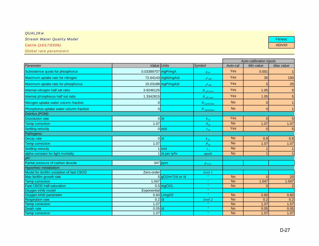
QUAL2Kw
Stream Water Quality Model Fitness:
Cattle (10/17/2006) #DIV/0!
Global rate parameters
Parameter Value Units Symbol Auto-cal Min value Max valueAuto-calibration inputs
Subsistence quota for phosphorus 0.03389707 mgP/mgA q 0P Yes 0.001 1
Maximum uptake rate for nitrogen 72.64143 mgN/mgA/d ρ mN Yes 35 150
Maximum uptake rate for phosphorus 15.03188 mgP/mgA/d ρ mP Yes 5 20
Internal nitrogen half sat ratio 3.9246125 K qN,ratio Yes 1.05 5
Internal phosphorus half sat ratio 1.3342815 K qP,ratio Yes 1.05 5
Nitrogen uptake water column fraction 0 N UpWCfrac No 0 1
Phosphorus uptake water column fraction 0 P UpWCfrac No 0 1Detritus (POM):Dissolution rate 0 /d k dt Yes 0 5Temp correction 1.07 θ dt No 1.07 1.07Settling velocity 0 m/d v dt Yes 0 5Pathogens:Decay rate 0 /d k dx No 0.8 0.8Temp correction 1.07 θ dx No 1.07 1.07Settling velocity 1 m/d v x No 1 1alpha constant for light mortality 1 /d per ly/hr apath No 1 1pH:Partial pressure of carbon dioxide 347 ppm p CO2
Hyporheic metabolismModel for biofilm oxidation of fast CBOD Zero-order level 1Max biofilm growth rate 5 gO2/m^2/d or /d " No 0 20Temp correction 1.047 " No 1.047 1.047Fast CBOD half-saturation 0.5 mgO2/L " No 0 2Oxygen inhib model Exponential "Oxygen inhib parameter 0.60 L/mgO2 " No 0.60 0.60Respiration rate 0.2 /d level 2 No 0.2 0.2Temp correction 1.07 " No 1.07 1.07Death rate 0.05 /d " No 0.05 0.05Temp correction 1.07 " No 1.07 1.07
D-27
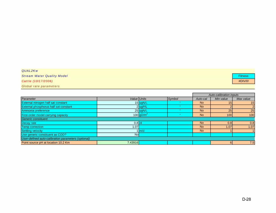
QUAL2Kw
Stream Water Quality Model Fitness:
Cattle (10/17/2006) #DIV/0!
Global rate parameters
Parameter Value Units Symbol Auto-cal Min value Max valueAuto-calibration inputs
External nitrogen half sat constant 15 ugN/L " No 15 15External phosphorus half sat constant 2 ugP/L " No 2 2Ammonia preference 25 ugN/L " No 25 25First-order model carrying capacity 100 gD/m2 " No 100 100Generic constituentDecay rate 0.8 /d No 0.8 0.8Temp correction 1.07 No 1.07 1.07Settling velocity 1 m/d No 1 1Use generic constituent as COD? NoUser-defined auto-calibration parameters (optional)Point source pH at location 10.2 Km 7.43916 6 7.5
D-28

QUAL2Kw
Stream Water Quality Model
Cattle (10/17/2006)
Global rate parameters
Random number seed 123456 seedModel runs in a population (<=512) 4 npGenerations in the evolution 2 ngenDigits to encode genotype (<=6) 5 ndCrossover mode (1, 2, 3, 4, 5, 6, or 7) 3 icrossCrossover probability (0-1): 0.85 pcrossMutation mode (1, 2, 3, 4, 5, or 6) 2 imutInitial mutation rate (0-1): 0.005 pmutMinimum mutation rate (0-1): 0.0005 pmutmnMaximum mutation rate (0-1): 0.25 pmutmxRelative fitness differential (0-1): 1 fdifReproduction plan (1, 2, or 3): 1 irepElitism (0 or 1): 1 ieliteRestart from previous evolution (0 or 1): 0 irestart
Auto-calibration genetic algorithm control:
D-29

Cattle (10/17/2006)
0.00
0.00
0.00
0.00
0.00
0.00
0.00
0.00
0.00
0.00
0.00
011223344distance upstream (Km)
flow
(m^3
/s)
Q, m3/s Q-data m3/s
D-30

Cattle (10/17/2006)
0
5
10
15
20
25
011223344distance upstream (Km)
tem
pera
ture
(deg
C)
Temp(C) Average Mean Temp-data Temp(C) MinimumTemp(C) Maximum Minimum Temp-data Maximum Temp-data
D-31

Cattle (10/17/2006)
0
1
2
3
4
5
6
7
8
9
10
11
12
13
0.000.501.001.502.002.503.003.504.00distance upstream (Km)
diss
olve
d ox
ygen
(mg/
L)
DO(mgO2/L) DO (mgO2/L) data DO(mgO2/L) Min DO(mgO2/L) MaxMinimum DO-data Maximum DO-data DO sat
D-32

Cattle (10/17/2006)
0
10
20
30
40
50
60
70
80
90
011223344distance upstream (Km)
fast
-reac
ting
CBOD
(mg/
L)
CBODf (mgO2/L) CBODf (mgO2/L) data CBODf (mgO2/L) Min CBODf (mgO2/L) Max
D-33

Cattle (10/17/2006)
0
200
400
600
800
1000
1200
1400
1600
011223344distance upstream (Km)
orga
nic N
(ugN
/L)
No(ugN/L) data No(ugN/L) Min No(ugN/L) Max Minimum No-data Maximum No-data
D-34

Cattle (10/17/2006)
0
100
200
300
400
500
600
700
011223344distance upstream (Km)
amm
onia
(ugN
/L)
NH4 (ugN/L) data NH4(ugN/L) NH4(ugN/L) MinNH4(ugN/L) Max Minimum NH4-data Maximum NH4-data
D-35

QUAL2Kw
Stream Water Quality Model
Chicken (10/18/1991)
Headwater and Downstream Boundary Data:
Headwater Flow 0.000 m3/sPrescribed downstream boundary? NoHeadwater Water Quality Units 12:00 AMTemperature C 20.00Conductivity umhos 0.00Inorganic Solids mgD/L 0.00Dissolved Oxygen mg/L 7.00CBODslow mgO2/L 1.00CBODfast mgO2/L 1.00Organic Nitrogen ugN/L 10.00NH4-Nitrogen ugN/L 10.00NO3-Nitrogen ugN/L 0.00Organic Phosphorus ugP/L 0.00Inorganic Phosphorus (SRP) ugP/L 0.00Phytoplankton ugA/L 0.00Detritus (POM) mgD/L 0.00Pathogen cfu/100 mL 0.00Generic constituent user defined 0.00Alkalinity mgCaCO3/L 200.00pH s.u. 7.33Downstream Boundary Water Quality (optional) Units 12:00 AM
D-36

QUAL2Kw
Stream Water Quality Model
Chicken (10/18/1991)
Reach Data:
Reach for diel plot: 11Reach Downstream
Reach Downstream length Downstream locationLabel end of reach label Number (km) Latitude Longitude (km)
Headwater 0 38.59 89.54 3.3001 0.30 38.59 89.54 3.0002 0.30 38.59 89.54 2.7003 0.30 38.59 89.54 2.4004 0.30 38.59 89.54 2.1005 0.30 38.59 89.54 1.8006 0.30 38.59 89.54 1.5007 0.30 38.59 89.54 1.2008 0.30 38.59 89.54 0.9009 0.30 38.59 89.54 0.600
10 0.30 38.59 89.54 0.30011 0.30 38.59 89.54 0.000
D-37

Number0123456789
1011
QUAL2Kw
Stream Water Quality Model
Chicken (10/18/1991)
Reach Data:
Upstream Downstream(m) (m) Degrees Minutes Seconds Degrees Minutes Seconds
149.000 38.00 35 0 89.00 32 0148.000 146.727 38.00 35 0 89.00 32 0146.727 145.455 38.00 35 0 89.00 32 0145.455 144.182 38.00 35 0 89.00 32 0144.182 142.909 38.00 35 0 89.00 32 0142.909 141.636 38.00 35 0 89.00 32 0141.636 140.364 38.00 35 0 89.00 32 0140.364 139.091 38.00 35 0 89.00 32 0139.091 137.818 38.00 35 0 89.00 32 0137.818 136.545 38.00 35 0 89.00 32 0136.545 135.273 38.00 35 0 89.00 32 0135.273 134.000 38.00 35 0 89.00 32 0
Elevation DownstreamLatitude Longitude
D-38

Number0123456789
1011
QUAL2Kw
Stream Water Quality Model
Chicken (10/18/1991)
Reach Data:
Hyd Hydraulic Model (Weir Overrides Rating Curves; Rating Curves Override Manning Formula Rating Curves
Height Width(m) (m) Coefficient Exponent Coefficient Exponent
0.0000 0.0000 0.0000 0.000 0.0000 0.0000.0000 0.0000 0.0000 0.000 0.0000 0.0000.0000 0.0000 0.0000 0.000 0.0000 0.0000.0000 0.0000 0.0000 0.000 0.0000 0.0000.0000 0.0000 0.0000 0.000 0.0000 0.0000.0000 0.0000 0.0000 0.000 0.0000 0.0000.0000 0.0000 0.0000 0.000 0.0000 0.0000.0000 0.0000 0.0000 0.000 0.0000 0.0000.0000 0.0000 0.0000 0.000 0.0000 0.0000.0000 0.0000 0.0000 0.000 0.0000 0.0000.0000 0.0000 0.0000 0.000 0.0000 0.0000.0000 0.0000 0.0000 0.000 0.0000 0.000
Velocity DepthWeir
D-39
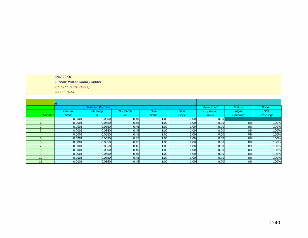
Number0123456789
1011
QUAL2Kw
Stream Water Quality Model
Chicken (10/18/1991)
Reach Data:
a) Manning Formula Prescribed Bottom Bottom
Channel Manning Bot Width Side Side Dispersion Algae SODSlope n m Slope Slope m2/s Coverage Coverage
0.0001 0.0550 0.45 1.00 1.00 0.000.0001 0.0550 0.45 1.00 1.00 0.00 0% 100%0.0001 0.0550 0.45 1.00 1.00 0.00 0% 100%0.0001 0.0550 0.45 1.00 1.00 0.00 0% 100%0.0001 0.0550 0.45 1.00 1.00 0.00 0% 100%0.0001 0.0550 0.45 1.00 1.00 0.00 0% 100%0.0001 0.0550 0.45 1.00 1.00 0.00 0% 100%0.0001 0.0550 0.45 1.00 1.00 0.00 0% 100%0.0001 0.0550 0.45 1.00 1.00 0.00 0% 100%0.0001 0.0550 0.45 1.00 1.00 0.00 0% 100%0.0001 0.0550 0.45 1.00 1.00 0.00 0% 100%0.0001 0.0550 0.45 1.00 1.00 0.00 0% 100%
D-40

Number0123456789
1011
QUAL2Kw
Stream Water Quality Model
Chicken (10/18/1991)
Reach Data:
Prescribed Prescribed Prescribed Prescribed Sediment Sediment Sediment/hyporheic Hyporheic HyporheicSOD CH4 flux NH4 flux Inorg P flux thermal cond thermal diff zone thickness exchange flow sediment porosity
gO2/m2/d gO2/m2/d mgN/m2/d mgP/m2/d (W/m/degC) (cm^2/sec) (cm) fraction of stream flow (fraction of volume)
5.00 0.0000 0.0000 0.0000 1.6 0.0064 10 5% 40%5.00 0.0000 0.0000 0.0000 1.6 0.0064 10 5% 40%5.00 0.0000 0.0000 0.0000 1.6 0.0064 10 5% 40%5.00 0.0000 0.0000 0.0000 1.6 0.0064 10 5% 40%5.00 0.0000 0.0000 0.0000 1.6 0.0064 10 5% 40%5.00 0.0000 0.0000 0.0000 1.6 0.0064 10 5% 40%5.00 0.0000 0.0000 0.0000 1.6 0.0064 10 5% 40%5.00 0.0000 0.0000 0.0000 1.6 0.0064 10 5% 40%5.00 0.0000 0.0000 0.0000 1.6 0.0064 10 5% 40%5.00 0.0000 0.0000 0.0000 1.6 0.0064 10 5% 40%5.00 0.0000 0.0000 0.0000 1.6 0.0064 10 5% 40%
D-41

QUAL2Kw
Stream Water Quality Model
Chicken (10/18/1991)
Air Temperature Data:
Upstream Downstream 12:00 AM 1:00 AM 2:00 AM 3:00 AM 4:00 AM
Upstream Reach Downstream Reach Distance Distance Hourly air temperature for each reach (degrees C)
Label Label Label Number km kmHeadwater 1 3.30 3.00 14.44 12.78 11.67 10.56 11.11
2 3.00 2.70 14.44 12.78 11.67 10.56 11.113 2.70 2.40 14.44 12.78 11.67 10.56 11.114 2.40 2.10 14.44 12.78 11.67 10.56 11.115 2.10 1.80 14.44 12.78 11.67 10.56 11.116 1.80 1.50 14.44 12.78 11.67 10.56 11.117 1.50 1.20 14.44 12.78 11.67 10.56 11.118 1.20 0.90 14.44 12.78 11.67 10.56 11.119 0.90 0.60 14.44 12.78 11.67 10.56 11.11
10 0.60 0.30 14.44 12.78 11.67 10.56 11.1111 0.30 0.00 14.44 12.78 11.67 10.56 11.11
(The input values are applied as point estimates at each time. Linear interpolation is used to estimate values between the hourly inputs.)
D-42

Reach
Number123456789
1011
QUAL2Kw
Stream Water Quality Model
Chicken (10/18/1991)
Air Temperature Data:
5:00 AM 6:00 AM 7:00 AM 8:00 AM 9:00 AM 10:00 AM 11:00 AM 12:00 PM 1:00 PM 2:00 PM
11.11 10.00 10.56 11.67 13.89 16.11 18.33 19.44 18.89 18.3311.11 10.00 10.56 11.67 13.89 16.11 18.33 19.44 18.89 18.3311.11 10.00 10.56 11.67 13.89 16.11 18.33 19.44 18.89 18.3311.11 10.00 10.56 11.67 13.89 16.11 18.33 19.44 18.89 18.3311.11 10.00 10.56 11.67 13.89 16.11 18.33 19.44 18.89 18.3311.11 10.00 10.56 11.67 13.89 16.11 18.33 19.44 18.89 18.3311.11 10.00 10.56 11.67 13.89 16.11 18.33 19.44 18.89 18.3311.11 10.00 10.56 11.67 13.89 16.11 18.33 19.44 18.89 18.3311.11 10.00 10.56 11.67 13.89 16.11 18.33 19.44 18.89 18.3311.11 10.00 10.56 11.67 13.89 16.11 18.33 19.44 18.89 18.3311.11 10.00 10.56 11.67 13.89 16.11 18.33 19.44 18.89 18.33
D-43
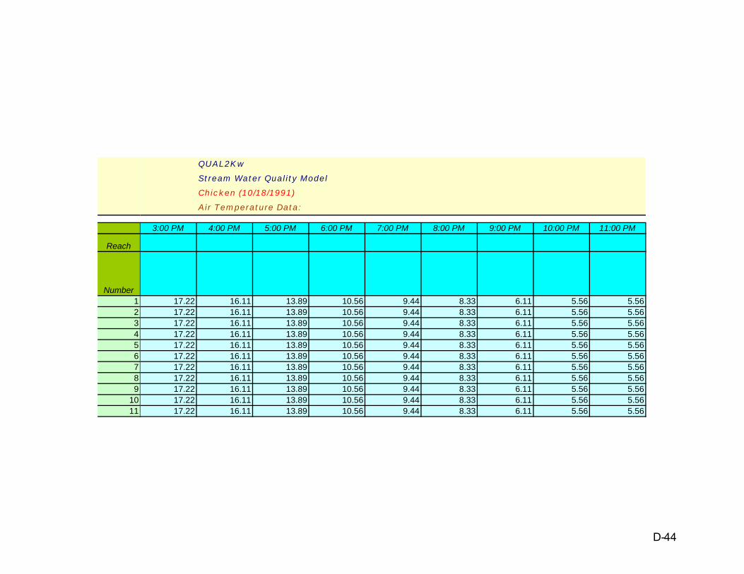
Reach
Number123456789
1011
QUAL2Kw
Stream Water Quality Model
Chicken (10/18/1991)
Air Temperature Data:
3:00 PM 4:00 PM 5:00 PM 6:00 PM 7:00 PM 8:00 PM 9:00 PM 10:00 PM 11:00 PM
17.22 16.11 13.89 10.56 9.44 8.33 6.11 5.56 5.5617.22 16.11 13.89 10.56 9.44 8.33 6.11 5.56 5.5617.22 16.11 13.89 10.56 9.44 8.33 6.11 5.56 5.5617.22 16.11 13.89 10.56 9.44 8.33 6.11 5.56 5.5617.22 16.11 13.89 10.56 9.44 8.33 6.11 5.56 5.5617.22 16.11 13.89 10.56 9.44 8.33 6.11 5.56 5.5617.22 16.11 13.89 10.56 9.44 8.33 6.11 5.56 5.5617.22 16.11 13.89 10.56 9.44 8.33 6.11 5.56 5.5617.22 16.11 13.89 10.56 9.44 8.33 6.11 5.56 5.5617.22 16.11 13.89 10.56 9.44 8.33 6.11 5.56 5.5617.22 16.11 13.89 10.56 9.44 8.33 6.11 5.56 5.56
D-44

QUAL2Kw
Stream Water Quality Model
Chicken (10/18/1991)
Dew Point Temperature Data:
Upstream Downstream 12:00 AM 1:00 AM 2:00 AM 3:00 AM 4:00 AMUpstream Reach Downstream Reach Distance Distance Hourly dewpoint temperature for each reach (degrees C)
Label Label Label Number km kmHeadwater 1 3.30 3.00 7.22 7.22 7.22 7.22 7.78
2 3.00 2.70 7.22 7.22 7.22 7.22 7.783 2.70 2.40 7.22 7.22 7.22 7.22 7.784 2.40 2.10 7.22 7.22 7.22 7.22 7.785 2.10 1.80 7.22 7.22 7.22 7.22 7.786 1.80 1.50 7.22 7.22 7.22 7.22 7.787 1.50 1.20 7.22 7.22 7.22 7.22 7.788 1.20 0.90 7.22 7.22 7.22 7.22 7.789 0.90 0.60 7.22 7.22 7.22 7.22 7.78
10 0.60 0.30 7.22 7.22 7.22 7.22 7.7811 0.30 0.00 7.22 7.22 7.22 7.22 7.78
(The input values are applied as point estimates at each time. Linear interpolation is used to estimate values between the hourly inputs.)
D-45
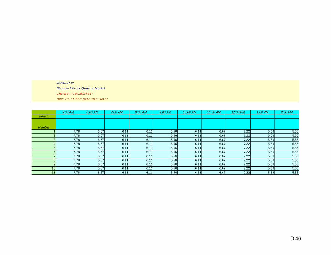
Reach
Number123456789
1011
QUAL2Kw
Stream Water Quality Model
Chicken (10/18/1991)
Dew Point Temperature Data:
5:00 AM 6:00 AM 7:00 AM 8:00 AM 9:00 AM 10:00 AM 11:00 AM 12:00 PM 1:00 PM 2:00 PM
7.78 6.67 6.11 6.11 5.56 6.11 6.67 7.22 5.56 5.567.78 6.67 6.11 6.11 5.56 6.11 6.67 7.22 5.56 5.567.78 6.67 6.11 6.11 5.56 6.11 6.67 7.22 5.56 5.567.78 6.67 6.11 6.11 5.56 6.11 6.67 7.22 5.56 5.567.78 6.67 6.11 6.11 5.56 6.11 6.67 7.22 5.56 5.567.78 6.67 6.11 6.11 5.56 6.11 6.67 7.22 5.56 5.567.78 6.67 6.11 6.11 5.56 6.11 6.67 7.22 5.56 5.567.78 6.67 6.11 6.11 5.56 6.11 6.67 7.22 5.56 5.567.78 6.67 6.11 6.11 5.56 6.11 6.67 7.22 5.56 5.567.78 6.67 6.11 6.11 5.56 6.11 6.67 7.22 5.56 5.567.78 6.67 6.11 6.11 5.56 6.11 6.67 7.22 5.56 5.56
D-46

Reach
Number123456789
1011
QUAL2Kw
Stream Water Quality Model
Chicken (10/18/1991)
Dew Point Temperature Data:
3:00 PM 4:00 PM 5:00 PM 6:00 PM 7:00 PM 8:00 PM 9:00 PM 10:00 PM 11:00 PM
5.00 3.33 3.33 1.11 1.11 2.78 4.44 5.56 5.565.00 3.33 3.33 1.11 1.11 2.78 4.44 5.56 5.565.00 3.33 3.33 1.11 1.11 2.78 4.44 5.56 5.565.00 3.33 3.33 1.11 1.11 2.78 4.44 5.56 5.565.00 3.33 3.33 1.11 1.11 2.78 4.44 5.56 5.565.00 3.33 3.33 1.11 1.11 2.78 4.44 5.56 5.565.00 3.33 3.33 1.11 1.11 2.78 4.44 5.56 5.565.00 3.33 3.33 1.11 1.11 2.78 4.44 5.56 5.565.00 3.33 3.33 1.11 1.11 2.78 4.44 5.56 5.565.00 3.33 3.33 1.11 1.11 2.78 4.44 5.56 5.565.00 3.33 3.33 1.11 1.11 2.78 4.44 5.56 5.56
D-47

QUAL2Kw
Stream Water Quality Model
Chicken (10/18/1991)
Wind Speed Data:
Upstream Downstream 12:00 AM 1:00 AM 2:00 AM 3:00 AM 4:00 AMUpstream Reach Downstream Reach Distance Distance Wind speed for each reach 7m above water surface (m/s)
Label Label Label Number km kmHeadwater 1 3.30 3.00 5.66 3.60 3.60 3.09 3.60
2 3.00 2.70 5.66 3.60 3.60 3.09 3.603 2.70 2.40 5.66 3.60 3.60 3.09 3.604 2.40 2.10 5.66 3.60 3.60 3.09 3.605 2.10 1.80 5.66 3.60 3.60 3.09 3.606 1.80 1.50 5.66 3.60 3.60 3.09 3.607 1.50 1.20 5.66 3.60 3.60 3.09 3.608 1.20 0.90 5.66 3.60 3.60 3.09 3.609 0.90 0.60 5.66 3.60 3.60 3.09 3.60
10 0.60 0.30 5.66 3.60 3.60 3.09 3.6011 0.30 0.00 5.66 3.60 3.60 3.09 3.60
(The input values are applied as point estimates at each time. Linear interpolation is used to estimate values between the hourly inputs.)
D-48
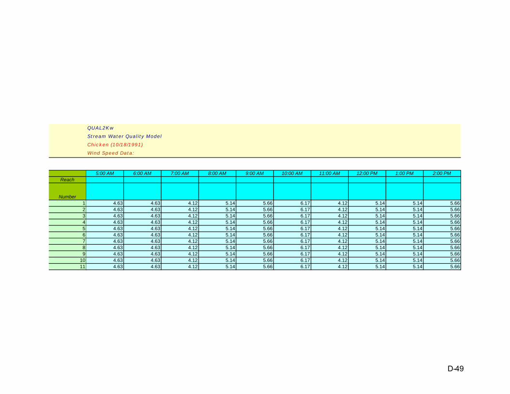
Reach
Number123456789
1011
QUAL2Kw
Stream Water Quality Model
Chicken (10/18/1991)
Wind Speed Data:
5:00 AM 6:00 AM 7:00 AM 8:00 AM 9:00 AM 10:00 AM 11:00 AM 12:00 PM 1:00 PM 2:00 PM
4.63 4.63 4.12 5.14 5.66 6.17 4.12 5.14 5.14 5.664.63 4.63 4.12 5.14 5.66 6.17 4.12 5.14 5.14 5.664.63 4.63 4.12 5.14 5.66 6.17 4.12 5.14 5.14 5.664.63 4.63 4.12 5.14 5.66 6.17 4.12 5.14 5.14 5.664.63 4.63 4.12 5.14 5.66 6.17 4.12 5.14 5.14 5.664.63 4.63 4.12 5.14 5.66 6.17 4.12 5.14 5.14 5.664.63 4.63 4.12 5.14 5.66 6.17 4.12 5.14 5.14 5.664.63 4.63 4.12 5.14 5.66 6.17 4.12 5.14 5.14 5.664.63 4.63 4.12 5.14 5.66 6.17 4.12 5.14 5.14 5.664.63 4.63 4.12 5.14 5.66 6.17 4.12 5.14 5.14 5.664.63 4.63 4.12 5.14 5.66 6.17 4.12 5.14 5.14 5.66
D-49

Reach
Number123456789
1011
QUAL2Kw
Stream Water Quality Model
Chicken (10/18/1991)
Wind Speed Data:
3:00 PM 4:00 PM 5:00 PM 6:00 PM 7:00 PM 8:00 PM 9:00 PM 10:00 PM 11:00 PM
5.14 7.72 7.72 11.32 7.72 8.23 6.69 4.63 6.175.14 7.72 7.72 11.32 7.72 8.23 6.69 4.63 6.175.14 7.72 7.72 11.32 7.72 8.23 6.69 4.63 6.175.14 7.72 7.72 11.32 7.72 8.23 6.69 4.63 6.175.14 7.72 7.72 11.32 7.72 8.23 6.69 4.63 6.175.14 7.72 7.72 11.32 7.72 8.23 6.69 4.63 6.175.14 7.72 7.72 11.32 7.72 8.23 6.69 4.63 6.175.14 7.72 7.72 11.32 7.72 8.23 6.69 4.63 6.175.14 7.72 7.72 11.32 7.72 8.23 6.69 4.63 6.175.14 7.72 7.72 11.32 7.72 8.23 6.69 4.63 6.175.14 7.72 7.72 11.32 7.72 8.23 6.69 4.63 6.17
D-50

QUAL2Kw
Stream Water Quality Model
Chicken (10/18/1991)
Cloud Cover Data:
Upstream Downstream 12:00 AM 1:00 AM 2:00 AM 3:00 AM 4:00 AMUpstream Reach Downstream Reach Distance Distance Hourly cloud cover shade for each reach (Percent)
Label Label Label Number km kmHeadwater 1 3.30 3.00 0.0% 0.0% 0.0% 0.0% 0.0%
2 3.00 2.70 0.0% 0.0% 0.0% 0.0% 0.0%3 2.70 2.40 0.0% 0.0% 0.0% 0.0% 0.0%4 2.40 2.10 0.0% 0.0% 0.0% 0.0% 0.0%5 2.10 1.80 0.0% 0.0% 0.0% 0.0% 0.0%6 1.80 1.50 0.0% 0.0% 0.0% 0.0% 0.0%7 1.50 1.20 0.0% 0.0% 0.0% 0.0% 0.0%8 1.20 0.90 0.0% 0.0% 0.0% 0.0% 0.0%9 0.90 0.60 0.0% 0.0% 0.0% 0.0% 0.0%
10 0.60 0.30 0.0% 0.0% 0.0% 0.0% 0.0%11 0.30 0.00 0.0% 0.0% 0.0% 0.0% 0.0%
(Percent of sky that is covered by clouds. The input values are applied as point estimates at each time. Linear interpolation is used to estimate values between the hourly inputs.)
D-51

Reach
Number123456789
1011
QUAL2Kw
Stream Water Quality Model
Chicken (10/18/1991)
Cloud Cover Data:
5:00 AM 6:00 AM 7:00 AM 8:00 AM 9:00 AM 10:00 AM 11:00 AM 12:00 PM 1:00 PM 2:00 PM
0.0% 0.0% 0.0% 0.0% 0.0% 0.0% 1.0% 7.0% 10.0% 9.0%0.0% 0.0% 0.0% 0.0% 0.0% 0.0% 1.0% 7.0% 10.0% 9.0%0.0% 0.0% 0.0% 0.0% 0.0% 0.0% 1.0% 7.0% 10.0% 9.0%0.0% 0.0% 0.0% 0.0% 0.0% 0.0% 1.0% 7.0% 10.0% 9.0%0.0% 0.0% 0.0% 0.0% 0.0% 0.0% 1.0% 7.0% 10.0% 9.0%0.0% 0.0% 0.0% 0.0% 0.0% 0.0% 1.0% 7.0% 10.0% 9.0%0.0% 0.0% 0.0% 0.0% 0.0% 0.0% 1.0% 7.0% 10.0% 9.0%0.0% 0.0% 0.0% 0.0% 0.0% 0.0% 1.0% 7.0% 10.0% 9.0%0.0% 0.0% 0.0% 0.0% 0.0% 0.0% 1.0% 7.0% 10.0% 9.0%0.0% 0.0% 0.0% 0.0% 0.0% 0.0% 1.0% 7.0% 10.0% 9.0%0.0% 0.0% 0.0% 0.0% 0.0% 0.0% 1.0% 7.0% 10.0% 9.0%
D-52

Reach
Number123456789
1011
QUAL2Kw
Stream Water Quality Model
Chicken (10/18/1991)
Cloud Cover Data:
3:00 PM 4:00 PM 5:00 PM 6:00 PM 7:00 PM 8:00 PM 9:00 PM 10:00 PM 11:00 PM
10.0% 10.0% 10.0% 10.0% 10.0% 10.0% 10.0% 10.0% 10.0%10.0% 10.0% 10.0% 10.0% 10.0% 10.0% 10.0% 10.0% 10.0%10.0% 10.0% 10.0% 10.0% 10.0% 10.0% 10.0% 10.0% 10.0%10.0% 10.0% 10.0% 10.0% 10.0% 10.0% 10.0% 10.0% 10.0%10.0% 10.0% 10.0% 10.0% 10.0% 10.0% 10.0% 10.0% 10.0%10.0% 10.0% 10.0% 10.0% 10.0% 10.0% 10.0% 10.0% 10.0%10.0% 10.0% 10.0% 10.0% 10.0% 10.0% 10.0% 10.0% 10.0%10.0% 10.0% 10.0% 10.0% 10.0% 10.0% 10.0% 10.0% 10.0%10.0% 10.0% 10.0% 10.0% 10.0% 10.0% 10.0% 10.0% 10.0%10.0% 10.0% 10.0% 10.0% 10.0% 10.0% 10.0% 10.0% 10.0%10.0% 10.0% 10.0% 10.0% 10.0% 10.0% 10.0% 10.0% 10.0%
D-53

QUAL2Kw
Stream Water Quality Model
Chicken (10/18/1991)
Shade Data:
Upstream Downstream 12:00 AM 1:00 AM 2:00 AM 3:00 AM 4:00 AMUpstream Reach Downstream Reach Distance Distance Integrated hourly effective shade for each reach (Percent)
Label Label Label Number km kmHeadwater 1 3.30 3.00 0.0% 0.0% 0.0% 0.0% 0.0%
2 3.00 2.70 0.0% 0.0% 0.0% 0.0% 0.0%3 2.70 2.40 0.0% 0.0% 0.0% 0.0% 0.0%4 2.40 2.10 0.0% 0.0% 0.0% 0.0% 0.0%5 2.10 1.80 0.0% 0.0% 0.0% 0.0% 0.0%6 1.80 1.50 0.0% 0.0% 0.0% 0.0% 0.0%7 1.50 1.20 0.0% 0.0% 0.0% 0.0% 0.0%8 1.20 0.90 0.0% 0.0% 0.0% 0.0% 0.0%9 0.90 0.60 0.0% 0.0% 0.0% 0.0% 0.0%
10 0.60 0.30 0.0% 0.0% 0.0% 0.0% 0.0%11 0.30 0.00 0.0% 0.0% 0.0% 0.0% 0.0%
(Percent of solar radiation that is blocked because of shade from topography and vegetation. Hourly values are applied as integrated values for each hour, e.g. the value at 12:00 AM is applied from 12:00 to 1:00 AM)
D-54

Reach
Number123456789
1011
QUAL2Kw
Stream Water Quality Model
Chicken (10/18/1991)
Shade Data:
5:00 AM 6:00 AM 7:00 AM 8:00 AM 9:00 AM 10:00 AM 11:00 AM 12:00 PM 1:00 PM 2:00 PM
0.0% 0.0% 0.0% 0.0% 0.0% 0.0% 0.0% 0.0% 0.0% 0.0%0.0% 0.0% 0.0% 0.0% 0.0% 0.0% 0.0% 0.0% 0.0% 0.0%0.0% 0.0% 0.0% 0.0% 0.0% 0.0% 0.0% 0.0% 0.0% 0.0%0.0% 0.0% 0.0% 0.0% 0.0% 0.0% 0.0% 0.0% 0.0% 0.0%0.0% 0.0% 0.0% 0.0% 0.0% 0.0% 0.0% 0.0% 0.0% 0.0%0.0% 0.0% 0.0% 0.0% 0.0% 0.0% 0.0% 0.0% 0.0% 0.0%0.0% 0.0% 0.0% 0.0% 0.0% 0.0% 0.0% 0.0% 0.0% 0.0%0.0% 0.0% 0.0% 0.0% 0.0% 0.0% 0.0% 0.0% 0.0% 0.0%0.0% 0.0% 0.0% 0.0% 0.0% 0.0% 0.0% 0.0% 0.0% 0.0%0.0% 0.0% 0.0% 0.0% 0.0% 0.0% 0.0% 0.0% 0.0% 0.0%0.0% 0.0% 0.0% 0.0% 0.0% 0.0% 0.0% 0.0% 0.0% 0.0%
D-55
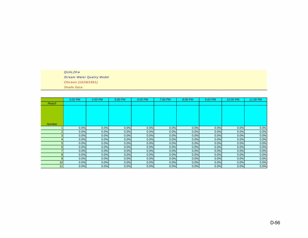
Reach
Number123456789
1011
QUAL2Kw
Stream Water Quality Model
Chicken (10/18/1991)
Shade Data:
3:00 PM 4:00 PM 5:00 PM 6:00 PM 7:00 PM 8:00 PM 9:00 PM 10:00 PM 11:00 PM
0.0% 0.0% 0.0% 0.0% 0.0% 0.0% 0.0% 0.0% 0.0%0.0% 0.0% 0.0% 0.0% 0.0% 0.0% 0.0% 0.0% 0.0%0.0% 0.0% 0.0% 0.0% 0.0% 0.0% 0.0% 0.0% 0.0%0.0% 0.0% 0.0% 0.0% 0.0% 0.0% 0.0% 0.0% 0.0%0.0% 0.0% 0.0% 0.0% 0.0% 0.0% 0.0% 0.0% 0.0%0.0% 0.0% 0.0% 0.0% 0.0% 0.0% 0.0% 0.0% 0.0%0.0% 0.0% 0.0% 0.0% 0.0% 0.0% 0.0% 0.0% 0.0%0.0% 0.0% 0.0% 0.0% 0.0% 0.0% 0.0% 0.0% 0.0%0.0% 0.0% 0.0% 0.0% 0.0% 0.0% 0.0% 0.0% 0.0%0.0% 0.0% 0.0% 0.0% 0.0% 0.0% 0.0% 0.0% 0.0%0.0% 0.0% 0.0% 0.0% 0.0% 0.0% 0.0% 0.0% 0.0%
D-56

QUAL2Kw
Stream Water Quality Model
Chicken (10/18/1991)
Light Parameters and Surface Heat Transfer Models:
Parameter Value UnitPhotosynthetically Available Radiation 0.47Background light extinction 0.2 /m k eb
Linear chlorophyll light extinction 0.0088 1/m-(ugA/L) α p
Nonlinear chlorophyll light extinction 0.054 1/m-(ugA/L) 2/3 α pn
ISS light extinction 0.052 1/m-(mgD/L) α ι
Detritus light extinction 0.174 1/m-(mgD/L) α ο
Macrophyte light extinction 0.015 1/m-(gD/m 3 ) α mac
Solar shortwave radiation modelAtmospheric attenuation model for solar Ryan-StolzenbachBras solar parameter (used if Bras solar model is selected)atmospheric turbidity coefficient (2=clear, 5=smoggy, default=2) 2 n fac
Ryan-Stolzenbach solar parameter (used if Ryan-Stolzenbach solar model is selected)atmospheric transmission coefficient (0.70-0.91, default 0.8) 0.8 a tc
Downwelling atmospheric longwave IR radiationatmospheric longwave emissivity model BruntEvaporation and air convection/conductionwind speed function for evaporation and air convection/conduction Brady-Graves-Geyer
D-57
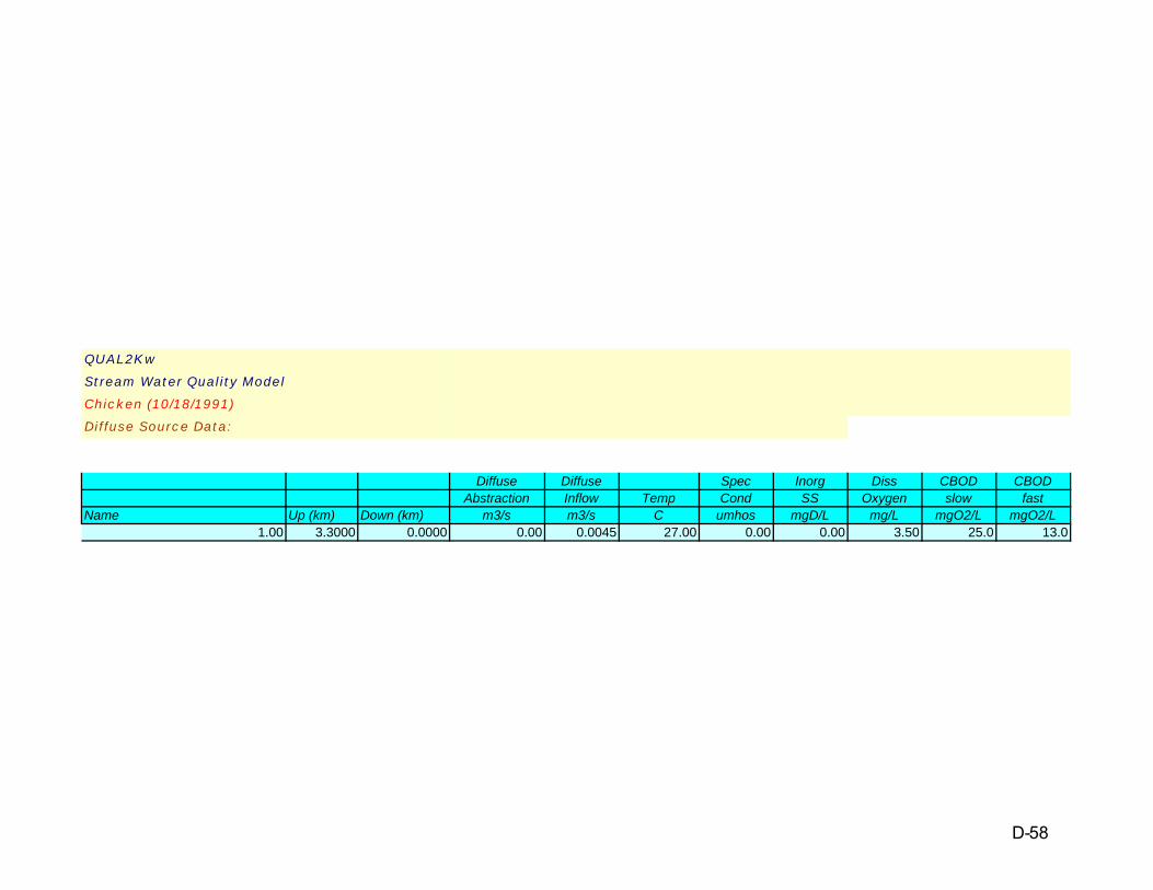
QUAL2Kw
Stream Water Quality Model
Chicken (10/18/1991)
Diffuse Source Data:
Diffuse Diffuse Spec Inorg Diss CBOD CBODAbstraction Inflow Temp Cond SS Oxygen slow fast
Name Up (km) Down (km) m3/s m3/s C umhos mgD/L mg/L mgO2/L mgO2/L1.00 3.3000 0.0000 0.00 0.0045 27.00 0.00 0.00 3.50 25.0 13.0
D-58

QUAL2Kw
Stream Water Quality Model
Chicken (10/18/1991)
Diffuse Source Data:
Organic Ammon Nitrate Organic Inorganic Phyto GenericN N N P P plankton Detritus Pathogen constituent Alk pH
ugN/L ugN/L ugN/L ugP/L ugP/L ug/L mgD/L cfu/100 mL user defined mgCaCO3/L4450.0 5300.0 0.0 0.0 0.0 0.0 0.0 0.0 0.0 100.0 7.0
D-59

QUAL2Kw
Stream Water Quality Model Fitness:
Chicken (10/18/1991) #DIV/0!
Global rate parameters
Parameter Value Units Symbol Auto-cal Min value Max valueStoichiometry:Carbon 40 gC gC No 30 50Nitrogen 7.2 gN gN No 3 9Phosphorus 1 gP gP No 0.4 2Dry weight 100 gD gD No 100 100Chlorophyll 1 gA gA No 0.4 2Inorganic suspended solids:Settling velocity 0.00236 m/d v i Yes 0 2Oxygen:Reaeration model O'Connor-Dobbins f(u h)Temp correction 1.024 θ a
Reaeration wind effect NoneO2 for carbon oxidation 2.69 gO2/gC r oc
O2 for NH4 nitrification 4.57 gO2/gN r on
Oxygen inhib model CBOD oxidation ExponentialOxygen inhib parameter CBOD oxidation 0.60 L/mgO2 K socf No 0.60 0.60Oxygen inhib model nitrification ExponentialOxygen inhib parameter nitrification 0.60 L/mgO2 K sona No 0.60 0.60Oxygen enhance model denitrification ExponentialOxygen enhance parameter denitrification 0.60 L/mgO2 K sodn No 0.60 0.60Oxygen inhib model phyto resp ExponentialOxygen inhib parameter phyto resp 0.60 L/mgO2 K sop No 0.60 0.60Oxygen enhance model bot alg resp ExponentialOxygen enhance parameter bot alg resp 0.60 L/mgO2 K sob No 0.60 0.60Slow CBOD:Hydrolysis rate 0.5 /d k hc Yes 0 5Temp correction 1.047 θ hc No 1 1.07Oxidation rate 0.1 /d k dcs Yes 0 5Temp correction 1.047 θ dcs No 1 1.07Fast CBOD:Oxidation rate 3.4 /d k dc Yes 0 5Temp correction 1.047 θ dc No 1 1.07Organic N:Hydrolysis 0.5 /d k hn Yes 0 5Temp correction 1.07 θ hn No 1 1.07Settling velocity 0.05 m/d v on Yes 0 2Ammonium:Nitrification 1 /d k na Yes 0 10Temp correction 1.07 θ na No 1 1.07Nitrate:Denitrification 0.1 /d k dn Yes 0 2Temp correction 1.07 θ dn No 1 1.07Sed denitrification transfer coeff 0.01 m/d v di Yes 0 1Temp correction 1.07 θ di No 1 1.07Organic P:Hydrolysis 0 /d k hp Yes 0 5Temp correction 1.07 θ hp No 1 1.07Settling velocity 0.84512 m/d v op Yes 0 2Inorganic P:Settling velocity 0 m/d v ip Yes 0 2Sed P oxygen attenuation half sat constant 0.65786 mgO2/L k spi Yes 0 2Phytoplankton:Max Growth rate 0 /d k gp No 1.5 3Temp correction 1.07 θ gp No 1 1.07Respiration rate 0 /d k rp No 0 1Temp correction 1.07 θ rp No 1 1.07Death rate 0 /d k dp No 0 1Temp correction 1 θ dp No 1 1.07Nitrogen half sat constant 15 ugN/L k sPp No 0 150Phosphorus half sat constant 2 ugP/L k sNp No 0 50Inorganic carbon half sat constant 1.30E-05 moles/L k sCp No 1.30E-06 1.30E-04Phytoplankton use HCO3- as substrate YesLight model Half saturationLight constant 57.6 langleys/d K Lp No 28.8 115.2
Auto-calibration inputs
D-60

QUAL2Kw
Stream Water Quality Model Fitness:
Chicken (10/18/1991) #DIV/0!
Global rate parameters
Parameter Value Units Symbol Auto-cal Min value Max valueAuto-calibration inputs
Ammonia preference 25 ugN/L k hnxp No 25 25Settling velocity 0.15 m/d v a No 0 5Bottom Plants:
Growth model Zero-order
Max Growth rate 0 mgA/m2/d or /d C gb Yes 0 500
Temp correction 1.07 θ gb No 1 1.07
First-order model carrying capacity 1000 mgA/m2 a b,max No 1000 1000
Respiration rate 0 /d k rb Yes 0 0.5
Temp correction 1.07 θ rb No 1 1.07
Excretion rate 0 /d k eb Yes 0 0.5
Temp correction 1.07 θ db No 1 1.07
Death rate 0 /d k db Yes 0 0.5
Temp correction 1.07 θ db No 1 1.07
External nitrogen half sat constant 0 ugN/L k sPb Yes 0 300
External phosphorus half sat constant 0 ugP/L k sNb Yes 0 100
Inorganic carbon half sat constant 2.50E-06 moles/L k sCb Yes 1.30E-06 1.30E-04
Bottom algae use HCO3- as substrate Yes
Light model Half saturation
Light constant 3.58588 langleys/d K Lb Yes 1 100
Ammonia preference 22.48993 ugN/L k hnxb Yes 1 100
Subsistence quota for nitrogen 0.63189468 mgN/mgA q 0N Yes 0.0072 7.2
Subsistence quota for phosphorus 0.03389707 mgP/mgA q 0P Yes 0.001 1
Maximum uptake rate for nitrogen 72.64143 mgN/mgA/d ρ mN Yes 35 150
Maximum uptake rate for phosphorus 15.03188 mgP/mgA/d ρ mP Yes 5 20
Internal nitrogen half sat ratio 3.9246125 K qN,ratio Yes 1.05 5
Internal phosphorus half sat ratio 1.3342815 K qP,ratio Yes 1.05 5
Nitrogen uptake water column fraction 0 N UpWCfrac No 0 1
Phosphorus uptake water column fraction 0 P UpWCfrac No 0 1Detritus (POM):Dissolution rate 0 /d k dt Yes 0 5Temp correction 1.07 θ dt No 1.07 1.07Settling velocity 0 m/d v dt Yes 0 5Pathogens:Decay rate 0 /d k dx No 0.8 0.8Temp correction 1.07 θ dx No 1.07 1.07Settling velocity 1 m/d v x No 1 1alpha constant for light mortality 1 /d per ly/hr apath No 1 1pH:Partial pressure of carbon dioxide 347 ppm p CO2
D-61
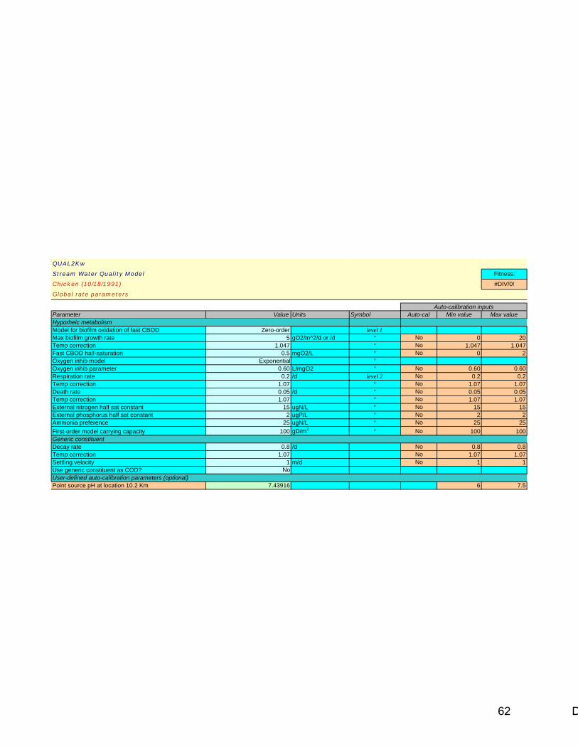
QUAL2Kw
Stream Water Quality Model Fitness:
Chicken (10/18/1991) #DIV/0!
Global rate parameters
Parameter Value Units Symbol Auto-cal Min value Max valueAuto-calibration inputs
Hyporheic metabolismModel for biofilm oxidation of fast CBOD Zero-order level 1Max biofilm growth rate 5 gO2/m^2/d or /d " No 0 20Temp correction 1.047 " No 1.047 1.047Fast CBOD half-saturation 0.5 mgO2/L " No 0 2Oxygen inhib model Exponential "Oxygen inhib parameter 0.60 L/mgO2 " No 0.60 0.60Respiration rate 0.2 /d level 2 No 0.2 0.2Temp correction 1.07 " No 1.07 1.07Death rate 0.05 /d " No 0.05 0.05Temp correction 1.07 " No 1.07 1.07External nitrogen half sat constant 15 ugN/L " No 15 15External phosphorus half sat constant 2 ugP/L " No 2 2Ammonia preference 25 ugN/L " No 25 25First-order model carrying capacity 100 gD/m2 " No 100 100Generic constituentDecay rate 0.8 /d No 0.8 0.8Temp correction 1.07 No 1.07 1.07Settling velocity 1 m/d No 1 1Use generic constituent as COD? NoUser-defined auto-calibration parameters (optional)Point source pH at location 10.2 Km 7.43916 6 7.5
D-62

QUAL2Kw
Stream Water Quality Model
Chicken (10/18/1991)
Global rate parameters
Random number seed 123456 seedModel runs in a population (<=512) 4 npGenerations in the evolution 2 ngenDigits to encode genotype (<=6) 5 ndCrossover mode (1, 2, 3, 4, 5, 6, or 7) 3 icrossCrossover probability (0-1): 0.85 pcrossMutation mode (1, 2, 3, 4, 5, or 6) 2 imutInitial mutation rate (0-1): 0.005 pmutMinimum mutation rate (0-1): 0.0005 pmutmnMaximum mutation rate (0-1): 0.25 pmutmxRelative fitness differential (0-1): 1 fdifReproduction plan (1, 2, or 3): 1 irepElitism (0 or 1): 1 ieliteRestart from previous evolution (0 or 1): 0 irestart
Auto-calibration genetic algorithm control:
D-63

Chicken (10/18/1991)
0.00
0.00
0.00
0.00
0.00
0.00
0.00
0.00
0.00
0.00
0.01
0112233distance upstream (Km)
flow
(m^3
/s)
Q, m3/s Q-data m3/s
D-64

Chicken (10/18/1991)
0
5
10
15
20
25
0112233distance upstream (Km)
tem
pera
ture
(deg
C)
Temp(C) Average Mean Temp-data Temp(C) MinimumTemp(C) Maximum Minimum Temp-data Maximum Temp-data
D-65

Chicken (10/18/1991)
0
1
2
3
4
5
6
7
8
9
10
11
12
13
0.000.501.001.502.002.503.00distance upstream (Km)
diss
olve
d ox
ygen
(mg/
L)
DO(mgO2/L) DO (mgO2/L) data DO(mgO2/L) Min DO(mgO2/L) MaxMinimum DO-data Maximum DO-data DO sat
D-66

Chicken (10/18/1991)
0
1
2
3
4
5
6
7
8
9
0112233distance upstream (Km)
fast
-reac
ting
CBOD
(mg/
L)
CBODf (mgO2/L) CBODf (mgO2/L) data CBODf (mgO2/L) Min CBODf (mgO2/L) Max
D-67

Chicken (10/18/1991)
0
500
1000
1500
2000
2500
3000
3500
0112233distance upstream (Km)
orga
nic N
(ugN
/L)
No(ugN/L) data No(ugN/L) Min No(ugN/L) Max Minimum No-data Maximum No-data
D-68

Chicken (10/18/1991)
0
500
1000
1500
2000
2500
3000
3500
4000
4500
5000
0112233distance upstream (Km)
amm
onia
(ugN
/L)
NH4 (ugN/L) data NH4(ugN/L) NH4(ugN/L) MinNH4(ugN/L) Max Minimum NH4-data Maximum NH4-data
D-69

QUAL2Kw
Stream Water Quality Model
Locust (10/17/2006)
Headwater and Downstream Boundary Data:
Headwater Flow 0.013 m3/sPrescribed downstream boundary? NoHeadwater Water Quality Units 12:00 AMTemperature C 14.00Conductivity umhos 0.00Inorganic Solids mgD/L 0.00Dissolved Oxygen mg/L 6.90CBODslow mgO2/L 7.70CBODfast mgO2/L 7.70Organic Nitrogen ugN/L 1250.00NH4-Nitrogen ugN/L 1250.00NO3-Nitrogen ugN/L 0.00Organic Phosphorus ugP/L 0.00Inorganic Phosphorus (SRP) ugP/L 0.00Phytoplankton ugA/L 0.00Detritus (POM) mgD/L 0.00Pathogen cfu/100 mL 0.00Generic constituent user defined 0.00Alkalinity mgCaCO3/L 200.00pH s.u. 7.33
D-70

QUAL2Kw
Stream Water Quality Model
Locust (10/17/2006)
Reach Data:
Reach for diel plot: 17Reach Downstream
Reach Downstream length Downstream location Upstream DownstreamLabel end of reach label Number (km) Latitude Longitude (km) (m) (m) Degrees Minutes Seconds Degrees Minutes Seconds
Headwater 0 38.59 89.54 7.250 150.000 38.00 35 0 89.00 32 01 0.25 38.59 89.54 7.000 149.286 148.571 38.00 35 0 89.00 32 02 0.25 38.59 89.54 6.750 148.571 147.857 38.00 35 0 89.00 32 03 0.25 38.59 89.54 6.500 147.857 147.143 38.00 35 0 89.00 32 04 0.25 38.59 89.54 6.250 147.143 146.429 38.00 35 0 89.00 32 05 0.25 38.59 89.54 6.000 146.429 145.714 38.00 35 0 89.00 32 06 0.25 38.59 89.54 5.750 145.714 145.000 38.00 35 0 89.00 32 07 0.25 38.59 89.54 5.500 145.000 144.286 38.00 35 0 89.00 32 08 0.25 38.59 89.54 5.250 144.286 143.571 38.00 35 0 89.00 32 09 0.25 38.59 89.54 5.000 143.571 142.857 38.00 35 0 89.00 32 010 0.25 38.59 89.54 4.750 142.857 142.143 38.00 35 0 89.00 32 011 0.25 38.59 89.54 4.500 142.143 141.429 38.00 35 0 89.00 32 012 0.25 38.59 89.54 4.250 141.429 140.714 38.00 35 0 89.00 32 013 0.25 38.59 89.54 4.000 140.714 140.286 38.00 35 0 89.00 32 014 0.25 38.59 89.54 3.750 140.286 139.857 38.00 35 0 89.00 32 015 0.25 38.59 89.54 3.500 139.857 139.429 38.00 35 0 89.00 32 016 0.25 38.59 89.54 3.250 139.429 139.000 38.00 35 0 89.00 32 017 0.25 38.59 89.54 3.000 139.000 138.571 38.00 35 0 89.00 32 018 0.25 38.59 89.54 2.750 138.571 138.143 38.00 35 0 89.00 32 019 0.25 38.59 89.54 2.500 138.143 137.714 38.00 35 0 89.00 32 020 0.25 38.59 89.54 2.250 137.714 137.286 38.00 35 0 89.00 32 021 0.25 38.59 89.54 2.000 137.286 136.857 38.00 35 0 89.00 32 022 0.25 38.59 89.54 1.750 136.857 136.429 38.00 35 0 89.00 32 023 0.25 38.59 89.54 1.500 136.429 136.000 38.00 35 0 89.00 32 024 0.25 38.59 89.54 1.250 136.000 135.571 38.00 35 0 89.00 32 025 0.25 38.59 89.54 1.000 135.571 135.143 38.00 35 0 89.00 32 026 0.25 38.59 89.54 0.750 135.143 134.714 38.00 35 0 89.00 32 027 0.25 38.59 89.54 0.500 134.714 134.286 38.00 35 0 89.00 32 028 0.25 38.59 89.54 0.250 134.286 134.286 38.00 35 0 89.00 32 029 0.25 38.59 89.54 0.000 134.286 134.286 38.00 35 0 89.00 32 0
Elevation DownstreamLatitude Longitude
D-71

Number01234567891011121314151617181920212223242526272829
QUAL2Kw
Stream Water Quality Model
Locust (10/17/2006)
Reach Data:
Hydraulic Model (Weir Overrides Rating Curves; Rating Curves Override Manning Formula) Rating Curves Manning Formula Prescribed Bottom
Height Width Channel Manning Bot Width Side Side Dispersion Algae(m) (m) Coefficient Exponent Coefficient Exponent Slope n m Slope Slope m2/s Coverage
0.0000 0.0000 0.0000 0.000 0.0000 0.000 0.000029 0.0500 3.03 2.00 2.00 0.000.0000 0.0000 0.0000 0.000 0.0000 0.000 0.000029 0.0500 3.03 2.00 2.00 0.00 0%0.0000 0.0000 0.0000 0.000 0.0000 0.000 0.000029 0.0500 3.03 2.00 2.00 0.00 0%0.0000 0.0000 0.0000 0.000 0.0000 0.000 0.000029 0.0500 3.03 2.00 2.00 0.00 0%0.0000 0.0000 0.0000 0.000 0.0000 0.000 0.000029 0.0500 3.03 2.00 2.00 0.00 0%0.0000 0.0000 0.0000 0.000 0.0000 0.000 0.000029 0.0500 3.03 2.00 2.00 0.00 0%0.0000 0.0000 0.0000 0.000 0.0000 0.000 0.000029 0.0500 3.03 2.00 2.00 0.00 0%0.0000 0.0000 0.0000 0.000 0.0000 0.000 0.000029 0.0500 3.03 2.00 2.00 0.00 0%0.0000 0.0000 0.0000 0.000 0.0000 0.000 0.000029 0.0500 3.03 2.00 2.00 0.00 0%0.0000 0.0000 0.0000 0.000 0.0000 0.000 0.000029 0.0500 3.03 2.00 2.00 0.00 0%0.0000 0.0000 0.0000 0.000 0.0000 0.000 0.000029 0.0500 3.03 2.00 2.00 0.00 0%0.0000 0.0000 0.0000 0.000 0.0000 0.000 0.000029 0.0500 3.03 2.00 2.00 0.00 0%0.0000 0.0000 0.0000 0.000 0.0000 0.000 0.000029 0.0500 3.03 2.00 2.00 0.00 0%0.0000 0.0000 0.0000 0.000 0.0000 0.000 0.000017 0.0500 3.03 2.00 2.00 0.00 0%0.0000 0.0000 0.0000 0.000 0.0000 0.000 0.000017 0.0500 3.03 2.00 2.00 0.00 0%0.0000 0.0000 0.0000 0.000 0.0000 0.000 0.000017 0.0500 3.03 2.00 2.00 0.00 0%0.0000 0.0000 0.0000 0.000 0.0000 0.000 0.000017 0.0500 3.03 2.00 2.00 0.00 0%0.0000 0.0000 0.0000 0.000 0.0000 0.000 0.000017 0.0500 3.03 2.00 2.00 0.00 0%0.0000 0.0000 0.0000 0.000 0.0000 0.000 0.000017 0.0500 3.03 2.00 2.00 1.00 0%0.0000 0.0000 0.0000 0.000 0.0000 0.000 0.000017 0.0500 3.03 2.00 2.00 2.00 0%0.0000 0.0000 0.0000 0.000 0.0000 0.000 0.000017 0.0500 3.03 2.00 2.00 3.00 0%0.0000 0.0000 0.0000 0.000 0.0000 0.000 0.000017 0.0500 3.03 2.00 2.00 4.00 0%0.0000 0.0000 0.0000 0.000 0.0000 0.000 0.000017 0.0500 3.03 2.00 2.00 5.00 0%0.0000 0.0000 0.0000 0.000 0.0000 0.000 0.000017 0.0500 3.03 2.00 2.00 6.00 0%0.0000 0.0000 0.0000 0.000 0.0000 0.000 0.000017 0.0500 3.03 2.00 2.00 7.00 0%0.0000 0.0000 0.0000 0.000 0.0000 0.000 0.000017 0.0500 3.03 2.00 2.00 8.00 0%0.0000 0.0000 0.0000 0.000 0.0000 0.000 0.000017 0.0500 3.03 2.00 2.00 9.00 0%0.0000 0.0000 0.0000 0.000 0.0000 0.000 0.000017 0.0500 3.03 2.00 2.00 10.00 0%0.0000 0.0000 0.0000 0.000 0.0000 0.000 0.000011 0.0500 3.03 2.00 2.00 11.00 0%0.0000 0.0000 0.0000 0.000 0.0000 0.000 0.000011 0.0500 3.03 2.00 2.00 12.00 0%
Velocity DepthWeir
D-72

Number01234567891011121314151617181920212223242526272829
QUAL2Kw
Stream Water Quality Model
Locust (10/17/2006)
Reach Data:
Bottom Prescribed Prescribed Prescribed Prescribed Sediment Sediment Sediment/hyporheic Hyporheic HyporheicSOD SOD CH4 flux NH4 flux Inorg P flux thermal cond thermal diff zone thickness exchange flow sediment porosity
Coverage gO2/m2/d gO2/m2/d mgN/m2/d mgP/m2/d (W/m/degC) (cm^2/sec) (cm) (fraction of stream flow) (fraction of volume)
100% 2.75 0.0000 0.0000 0.0000 1.6 0.0064 10 5% 40%100% 2.75 0.0000 0.0000 0.0000 1.6 0.0064 10 5% 40%100% 2.75 0.0000 0.0000 0.0000 1.6 0.0064 10 5% 40%100% 2.75 0.0000 0.0000 0.0000 1.6 0.0064 10 5% 40%100% 2.75 0.0000 0.0000 0.0000 1.6 0.0064 10 5% 40%100% 2.75 0.0000 0.0000 0.0000 1.6 0.0064 10 5% 40%100% 2.75 0.0000 0.0000 0.0000 1.6 0.0064 10 5% 40%100% 2.75 0.0000 0.0000 0.0000 1.6 0.0064 10 5% 40%100% 2.75 0.0000 0.0000 0.0000 1.6 0.0064 10 5% 40%100% 2.75 0.0000 0.0000 0.0000 1.6 0.0064 10 5% 40%100% 2.75 0.0000 0.0000 0.0000 1.6 0.0064 10 5% 40%100% 2.75 0.0000 0.0000 0.0000 1.6 0.0064 10 5% 40%100% 2.75 0.0000 0.0000 0.0000 1.6 0.0064 10 5% 40%100% 2.75 0.0000 0.0000 0.0000 1.6 0.0064 10 5% 40%100% 2.75 0.0000 0.0000 0.0000 1.6 0.0064 10 5% 40%100% 2.75 0.0000 0.0000 0.0000 1.6 0.0064 10 5% 40%100% 2.75 0.0000 0.0000 0.0000 1.6 0.0064 10 5% 40%100% 2.75 0.0000 0.0000 0.0000 1.6 0.0064 10 5% 40%100% 2.75 0.0000 0.0000 0.0000 1.6 0.0064 10 5% 40%100% 2.75 0.0000 0.0000 0.0000 1.6 0.0064 10 5% 40%100% 2.75 0.0000 0.0000 0.0000 1.6 0.0064 10 5% 40%100% 2.75 0.0000 0.0000 0.0000 1.6 0.0064 10 5% 40%100% 2.75 0.0000 0.0000 0.0000 1.6 0.0064 10 5% 40%100% 2.75 0.0000 0.0000 0.0000 1.6 0.0064 10 5% 40%100% 2.75 0.0000 0.0000 0.0000 1.6 0.0064 10 5% 40%100% 2.75 0.0000 0.0000 0.0000 1.6 0.0064 10 5% 40%100% 2.75 0.0000 0.0000 0.0000 1.6 0.0064 10 5% 40%100% 2.75 0.0000 0.0000 0.0000 1.6 0.0064 10 5% 40%100% 2.75 0.0000 0.0000 0.0000 1.6 0.0064 10 5% 40%
D-73

QUAL2Kw
Stream Water Quality Model
Locust (10/17/2006)
Air Temperature Data:
Upstream Downstream 12:00 AM 1:00 AM 2:00 AM 3:00 AM 4:00 AMUpstream Reach Downstream Reach Distance Distance Hourly air temperature for each reach (degrees C)
Label Label Label Number km kmHeadwater 1 7.25 7.00 13.00 14.00 16.00 16.00 14.00
2 7.00 6.75 13.00 14.00 16.00 16.00 14.003 6.75 6.50 13.00 14.00 16.00 16.00 14.004 6.50 6.25 13.00 14.00 16.00 16.00 14.005 6.25 6.00 13.00 14.00 16.00 16.00 14.006 6.00 5.75 13.00 14.00 16.00 16.00 14.007 5.75 5.50 13.00 14.00 16.00 16.00 14.008 5.50 5.25 13.00 14.00 16.00 16.00 14.009 5.25 5.00 13.00 14.00 16.00 16.00 14.00
10 5.00 4.75 13.00 14.00 16.00 16.00 14.0011 4.75 4.50 13.00 14.00 16.00 16.00 14.0012 4.50 4.25 13.00 14.00 16.00 16.00 14.0013 4.25 4.00 13.00 14.00 16.00 16.00 14.0014 4.00 3.75 13.00 14.00 16.00 16.00 14.0015 3.75 3.50 13.00 14.00 16.00 16.00 14.0016 3.50 3.25 13.00 14.00 16.00 16.00 14.0017 3.25 3.00 13.00 14.00 16.00 16.00 14.0018 3.00 2.75 13.00 14.00 16.00 16.00 14.0019 2.75 2.50 13.00 14.00 16.00 16.00 14.0020 2.50 2.25 13.00 14.00 16.00 16.00 14.0021 2.25 2.00 13.00 14.00 16.00 16.00 14.0022 2.00 1.75 13.00 14.00 16.00 16.00 14.0023 1.75 1.50 13.00 14.00 16.00 16.00 14.0024 1.50 1.25 13.00 14.00 16.00 16.00 14.0025 1.25 1.00 13.00 14.00 16.00 16.00 14.0026 1.00 0.75 13.00 14.00 16.00 16.00 14.0027 0.75 0.50 13.00 14.00 16.00 16.00 14.0028 0.50 0.25 13.00 14.00 16.00 16.00 14.0029 0.25 0.00 13.00 14.00 16.00 16.00 14.00
(The input values are applied as point estimates at each time. Linear interpolation is used to estimate values between the hourly inputs.)
D-74

Reach
Number123456789
1011121314151617181920212223242526272829
QUAL2Kw
Stream Water Quality Model
Locust (10/17/2006)
Air Temperature Data:
5:00 AM 6:00 AM 7:00 AM 8:00 AM 9:00 AM 10:00 AM 11:00 AM 12:00 PM 1:00 PM 2:00 PM
13.00 13.00 13.00 13.00 13.00 14.00 14.00 15.00 16.00 16.0013.00 13.00 13.00 13.00 13.00 14.00 14.00 15.00 16.00 16.0013.00 13.00 13.00 13.00 13.00 14.00 14.00 15.00 16.00 16.0013.00 13.00 13.00 13.00 13.00 14.00 14.00 15.00 16.00 16.0013.00 13.00 13.00 13.00 13.00 14.00 14.00 15.00 16.00 16.0013.00 13.00 13.00 13.00 13.00 14.00 14.00 15.00 16.00 16.0013.00 13.00 13.00 13.00 13.00 14.00 14.00 15.00 16.00 16.0013.00 13.00 13.00 13.00 13.00 14.00 14.00 15.00 16.00 16.0013.00 13.00 13.00 13.00 13.00 14.00 14.00 15.00 16.00 16.0013.00 13.00 13.00 13.00 13.00 14.00 14.00 15.00 16.00 16.0013.00 13.00 13.00 13.00 13.00 14.00 14.00 15.00 16.00 16.0013.00 13.00 13.00 13.00 13.00 14.00 14.00 15.00 16.00 16.0013.00 13.00 13.00 13.00 13.00 14.00 14.00 15.00 16.00 16.0013.00 13.00 13.00 13.00 13.00 14.00 14.00 15.00 16.00 16.0013.00 13.00 13.00 13.00 13.00 14.00 14.00 15.00 16.00 16.0013.00 13.00 13.00 13.00 13.00 14.00 14.00 15.00 16.00 16.0013.00 13.00 13.00 13.00 13.00 14.00 14.00 15.00 16.00 16.0013.00 13.00 13.00 13.00 13.00 14.00 14.00 15.00 16.00 16.0013.00 13.00 13.00 13.00 13.00 14.00 14.00 15.00 16.00 16.0013.00 13.00 13.00 13.00 13.00 14.00 14.00 15.00 16.00 16.0013.00 13.00 13.00 13.00 13.00 14.00 14.00 15.00 16.00 16.0013.00 13.00 13.00 13.00 13.00 14.00 14.00 15.00 16.00 16.0013.00 13.00 13.00 13.00 13.00 14.00 14.00 15.00 16.00 16.0013.00 13.00 13.00 13.00 13.00 14.00 14.00 15.00 16.00 16.0013.00 13.00 13.00 13.00 13.00 14.00 14.00 15.00 16.00 16.0013.00 13.00 13.00 13.00 13.00 14.00 14.00 15.00 16.00 16.0013.00 13.00 13.00 13.00 13.00 14.00 14.00 15.00 16.00 16.0013.00 13.00 13.00 13.00 13.00 14.00 14.00 15.00 16.00 16.0013.00 13.00 13.00 13.00 13.00 14.00 14.00 15.00 16.00 16.00
D-75

Reach
Number123456789
1011121314151617181920212223242526272829
QUAL2Kw
Stream Water Quality Model
Locust (10/17/2006)
Air Temperature Data:
3:00 PM 4:00 PM 5:00 PM 6:00 PM 7:00 PM 8:00 PM 9:00 PM 10:00 PM 11:00 PM
16.00 16.00 15.00 15.00 15.00 14.00 15.00 14.00 14.0016.00 16.00 15.00 15.00 15.00 14.00 15.00 14.00 14.0016.00 16.00 15.00 15.00 15.00 14.00 15.00 14.00 14.0016.00 16.00 15.00 15.00 15.00 14.00 15.00 14.00 14.0016.00 16.00 15.00 15.00 15.00 14.00 15.00 14.00 14.0016.00 16.00 15.00 15.00 15.00 14.00 15.00 14.00 14.0016.00 16.00 15.00 15.00 15.00 14.00 15.00 14.00 14.0016.00 16.00 15.00 15.00 15.00 14.00 15.00 14.00 14.0016.00 16.00 15.00 15.00 15.00 14.00 15.00 14.00 14.0016.00 16.00 15.00 15.00 15.00 14.00 15.00 14.00 14.0016.00 16.00 15.00 15.00 15.00 14.00 15.00 14.00 14.0016.00 16.00 15.00 15.00 15.00 14.00 15.00 14.00 14.0016.00 16.00 15.00 15.00 15.00 14.00 15.00 14.00 14.0016.00 16.00 15.00 15.00 15.00 14.00 15.00 14.00 14.0016.00 16.00 15.00 15.00 15.00 14.00 15.00 14.00 14.0016.00 16.00 15.00 15.00 15.00 14.00 15.00 14.00 14.0016.00 16.00 15.00 15.00 15.00 14.00 15.00 14.00 14.0016.00 16.00 15.00 15.00 15.00 14.00 15.00 14.00 14.0016.00 16.00 15.00 15.00 15.00 14.00 15.00 14.00 14.0016.00 16.00 15.00 15.00 15.00 14.00 15.00 14.00 14.0016.00 16.00 15.00 15.00 15.00 14.00 15.00 14.00 14.0016.00 16.00 15.00 15.00 15.00 14.00 15.00 14.00 14.0016.00 16.00 15.00 15.00 15.00 14.00 15.00 14.00 14.0016.00 16.00 15.00 15.00 15.00 14.00 15.00 14.00 14.0016.00 16.00 15.00 15.00 15.00 14.00 15.00 14.00 14.0016.00 16.00 15.00 15.00 15.00 14.00 15.00 14.00 14.0016.00 16.00 15.00 15.00 15.00 14.00 15.00 14.00 14.0016.00 16.00 15.00 15.00 15.00 14.00 15.00 14.00 14.0016.00 16.00 15.00 15.00 15.00 14.00 15.00 14.00 14.00
D-76

QUAL2Kw
Stream Water Quality Model
Locust (10/17/2006)
Dew Point Temperature Data:
Upstream Downstream 12:00 AM 1:00 AM 2:00 AM 3:00 AM 4:00 AM 5:00 AM 6:00 AM 7:00 AMUpstream Reach Downstream Reach Distance Distance Hourly dewpoint temperature for each reach (degrees C)
Label Label Label Number km kmHeadwater 1 7.25 7.00 12.00 13.00 15.00 14.00 12.00 11.00 11.00 11.00
2 7.00 6.75 12.00 13.00 15.00 14.00 12.00 11.00 11.00 11.003 6.75 6.50 12.00 13.00 15.00 14.00 12.00 11.00 11.00 11.004 6.50 6.25 12.00 13.00 15.00 14.00 12.00 11.00 11.00 11.005 6.25 6.00 12.00 13.00 15.00 14.00 12.00 11.00 11.00 11.006 6.00 5.75 12.00 13.00 15.00 14.00 12.00 11.00 11.00 11.007 5.75 5.50 12.00 13.00 15.00 14.00 12.00 11.00 11.00 11.008 5.50 5.25 12.00 13.00 15.00 14.00 12.00 11.00 11.00 11.009 5.25 5.00 12.00 13.00 15.00 14.00 12.00 11.00 11.00 11.00
10 5.00 4.75 12.00 13.00 15.00 14.00 12.00 11.00 11.00 11.0011 4.75 4.50 12.00 13.00 15.00 14.00 12.00 11.00 11.00 11.0012 4.50 4.25 12.00 13.00 15.00 14.00 12.00 11.00 11.00 11.0013 4.25 4.00 12.00 13.00 15.00 14.00 12.00 11.00 11.00 11.0014 4.00 3.75 12.00 13.00 15.00 14.00 12.00 11.00 11.00 11.0015 3.75 3.50 12.00 13.00 15.00 14.00 12.00 11.00 11.00 11.0016 3.50 3.25 12.00 13.00 15.00 14.00 12.00 11.00 11.00 11.0017 3.25 3.00 12.00 13.00 15.00 14.00 12.00 11.00 11.00 11.0018 3.00 2.75 12.00 13.00 15.00 14.00 12.00 11.00 11.00 11.0019 2.75 2.50 12.00 13.00 15.00 14.00 12.00 11.00 11.00 11.0020 2.50 2.25 12.00 13.00 15.00 14.00 12.00 11.00 11.00 11.0021 2.25 2.00 12.00 13.00 15.00 14.00 12.00 11.00 11.00 11.0022 2.00 1.75 12.00 13.00 15.00 14.00 12.00 11.00 11.00 11.0023 1.75 1.50 12.00 13.00 15.00 14.00 12.00 11.00 11.00 11.0024 1.50 1.25 12.00 13.00 15.00 14.00 12.00 11.00 11.00 11.0025 1.25 1.00 12.00 13.00 15.00 14.00 12.00 11.00 11.00 11.0026 1.00 0.75 12.00 13.00 15.00 14.00 12.00 11.00 11.00 11.0027 0.75 0.50 12.00 13.00 15.00 14.00 12.00 11.00 11.00 11.0028 0.50 0.25 12.00 13.00 15.00 14.00 12.00 11.00 11.00 11.0029 0.25 0.00 12.00 13.00 15.00 14.00 12.00 11.00 11.00 11.00
(The input values are applied as point estimates at each time. Linear interpolation is used to estimate values between the hourly inputs.)
D-77

Reach
Number123456789
1011121314151617181920212223242526272829
QUAL2Kw
Stream Water Quality Model
Locust (10/17/2006)
Dew Point Temperature Data:
8:00 AM 9:00 AM 10:00 AM 11:00 AM 12:00 PM 1:00 PM 2:00 PM 3:00 PM 4:00 PM 5:00 PM 6:00 PM 7:00 PM 8:00 PM 9:00 PM 10:00 PM 11:00 PM
11.00 11.00 12.00 12.00 12.00 12.00 13.00 13.00 13.00 13.00 13.00 13.00 13.00 13.00 13.00 13.0011.00 11.00 12.00 12.00 12.00 12.00 13.00 13.00 13.00 13.00 13.00 13.00 13.00 13.00 13.00 13.0011.00 11.00 12.00 12.00 12.00 12.00 13.00 13.00 13.00 13.00 13.00 13.00 13.00 13.00 13.00 13.0011.00 11.00 12.00 12.00 12.00 12.00 13.00 13.00 13.00 13.00 13.00 13.00 13.00 13.00 13.00 13.0011.00 11.00 12.00 12.00 12.00 12.00 13.00 13.00 13.00 13.00 13.00 13.00 13.00 13.00 13.00 13.0011.00 11.00 12.00 12.00 12.00 12.00 13.00 13.00 13.00 13.00 13.00 13.00 13.00 13.00 13.00 13.0011.00 11.00 12.00 12.00 12.00 12.00 13.00 13.00 13.00 13.00 13.00 13.00 13.00 13.00 13.00 13.0011.00 11.00 12.00 12.00 12.00 12.00 13.00 13.00 13.00 13.00 13.00 13.00 13.00 13.00 13.00 13.0011.00 11.00 12.00 12.00 12.00 12.00 13.00 13.00 13.00 13.00 13.00 13.00 13.00 13.00 13.00 13.0011.00 11.00 12.00 12.00 12.00 12.00 13.00 13.00 13.00 13.00 13.00 13.00 13.00 13.00 13.00 13.0011.00 11.00 12.00 12.00 12.00 12.00 13.00 13.00 13.00 13.00 13.00 13.00 13.00 13.00 13.00 13.0011.00 11.00 12.00 12.00 12.00 12.00 13.00 13.00 13.00 13.00 13.00 13.00 13.00 13.00 13.00 13.0011.00 11.00 12.00 12.00 12.00 12.00 13.00 13.00 13.00 13.00 13.00 13.00 13.00 13.00 13.00 13.0011.00 11.00 12.00 12.00 12.00 12.00 13.00 13.00 13.00 13.00 13.00 13.00 13.00 13.00 13.00 13.0011.00 11.00 12.00 12.00 12.00 12.00 13.00 13.00 13.00 13.00 13.00 13.00 13.00 13.00 13.00 13.0011.00 11.00 12.00 12.00 12.00 12.00 13.00 13.00 13.00 13.00 13.00 13.00 13.00 13.00 13.00 13.0011.00 11.00 12.00 12.00 12.00 12.00 13.00 13.00 13.00 13.00 13.00 13.00 13.00 13.00 13.00 13.0011.00 11.00 12.00 12.00 12.00 12.00 13.00 13.00 13.00 13.00 13.00 13.00 13.00 13.00 13.00 13.0011.00 11.00 12.00 12.00 12.00 12.00 13.00 13.00 13.00 13.00 13.00 13.00 13.00 13.00 13.00 13.0011.00 11.00 12.00 12.00 12.00 12.00 13.00 13.00 13.00 13.00 13.00 13.00 13.00 13.00 13.00 13.0011.00 11.00 12.00 12.00 12.00 12.00 13.00 13.00 13.00 13.00 13.00 13.00 13.00 13.00 13.00 13.0011.00 11.00 12.00 12.00 12.00 12.00 13.00 13.00 13.00 13.00 13.00 13.00 13.00 13.00 13.00 13.0011.00 11.00 12.00 12.00 12.00 12.00 13.00 13.00 13.00 13.00 13.00 13.00 13.00 13.00 13.00 13.0011.00 11.00 12.00 12.00 12.00 12.00 13.00 13.00 13.00 13.00 13.00 13.00 13.00 13.00 13.00 13.0011.00 11.00 12.00 12.00 12.00 12.00 13.00 13.00 13.00 13.00 13.00 13.00 13.00 13.00 13.00 13.0011.00 11.00 12.00 12.00 12.00 12.00 13.00 13.00 13.00 13.00 13.00 13.00 13.00 13.00 13.00 13.0011.00 11.00 12.00 12.00 12.00 12.00 13.00 13.00 13.00 13.00 13.00 13.00 13.00 13.00 13.00 13.0011.00 11.00 12.00 12.00 12.00 12.00 13.00 13.00 13.00 13.00 13.00 13.00 13.00 13.00 13.00 13.0011.00 11.00 12.00 12.00 12.00 12.00 13.00 13.00 13.00 13.00 13.00 13.00 13.00 13.00 13.00 13.00
D-78

QUAL2Kw
Stream Water Quality Model
Locust (10/17/2006)
Wind Speed Data:
Upstream Downstream 12:00 AM 1:00 AM 2:00 AM 3:00 AM 4:00 AM 5:00 AMUpstream Reach Downstream Reach Distance Distance Wind speed for each reach 7m above water surface (m/s)
Label Label Label Number km kmHeadwater 1 7.25 7.00 4.02 4.02 3.58 7.15 8.94 3.58
2 7.00 6.75 4.02 4.02 3.58 7.15 8.94 3.583 6.75 6.50 4.02 4.02 3.58 7.15 8.94 3.584 6.50 6.25 4.02 4.02 3.58 7.15 8.94 3.585 6.25 6.00 4.02 4.02 3.58 7.15 8.94 3.586 6.00 5.75 4.02 4.02 3.58 7.15 8.94 3.587 5.75 5.50 4.02 4.02 3.58 7.15 8.94 3.588 5.50 5.25 4.02 4.02 3.58 7.15 8.94 3.589 5.25 5.00 4.02 4.02 3.58 7.15 8.94 3.58
10 5.00 4.75 4.02 4.02 3.58 7.15 8.94 3.5811 4.75 4.50 4.02 4.02 3.58 7.15 8.94 3.5812 4.50 4.25 4.02 4.02 3.58 7.15 8.94 3.5813 4.25 4.00 4.02 4.02 3.58 7.15 8.94 3.5814 4.00 3.75 4.02 4.02 3.58 7.15 8.94 3.5815 3.75 3.50 4.02 4.02 3.58 7.15 8.94 3.5816 3.50 3.25 4.02 4.02 3.58 7.15 8.94 3.5817 3.25 3.00 4.02 4.02 3.58 7.15 8.94 3.5818 3.00 2.75 4.02 4.02 3.58 7.15 8.94 3.5819 2.75 2.50 4.02 4.02 3.58 7.15 8.94 3.5820 2.50 2.25 4.02 4.02 3.58 7.15 8.94 3.5821 2.25 2.00 4.02 4.02 3.58 7.15 8.94 3.5822 2.00 1.75 4.02 4.02 3.58 7.15 8.94 3.5823 1.75 1.50 4.02 4.02 3.58 7.15 8.94 3.5824 1.50 1.25 4.02 4.02 3.58 7.15 8.94 3.5825 1.25 1.00 4.02 4.02 3.58 7.15 8.94 3.5826 1.00 0.75 4.02 4.02 3.58 7.15 8.94 3.5827 0.75 0.50 4.02 4.02 3.58 7.15 8.94 3.5828 0.50 0.25 4.02 4.02 3.58 7.15 8.94 3.5829 0.25 0.00 4.02 4.02 3.58 7.15 8.94 3.58
(The input values are applied as point estimates at each time. Linear interpolation is used to estimate values between the hourly inputs.)
D-79

Reach
Number123456789
1011121314151617181920212223242526272829
QUAL2Kw
Stream Water Quality Model
Locust (10/17/2006)
Wind Speed Data:
6:00 AM 7:00 AM 8:00 AM 9:00 AM 10:00 AM 11:00 AM 12:00 PM 1:00 PM
4.47 2.68 4.02 4.02 3.58 3.58 2.68 3.134.47 2.68 4.02 4.02 3.58 3.58 2.68 3.134.47 2.68 4.02 4.02 3.58 3.58 2.68 3.134.47 2.68 4.02 4.02 3.58 3.58 2.68 3.134.47 2.68 4.02 4.02 3.58 3.58 2.68 3.134.47 2.68 4.02 4.02 3.58 3.58 2.68 3.134.47 2.68 4.02 4.02 3.58 3.58 2.68 3.134.47 2.68 4.02 4.02 3.58 3.58 2.68 3.134.47 2.68 4.02 4.02 3.58 3.58 2.68 3.134.47 2.68 4.02 4.02 3.58 3.58 2.68 3.134.47 2.68 4.02 4.02 3.58 3.58 2.68 3.134.47 2.68 4.02 4.02 3.58 3.58 2.68 3.134.47 2.68 4.02 4.02 3.58 3.58 2.68 3.134.47 2.68 4.02 4.02 3.58 3.58 2.68 3.134.47 2.68 4.02 4.02 3.58 3.58 2.68 3.134.47 2.68 4.02 4.02 3.58 3.58 2.68 3.134.47 2.68 4.02 4.02 3.58 3.58 2.68 3.134.47 2.68 4.02 4.02 3.58 3.58 2.68 3.134.47 2.68 4.02 4.02 3.58 3.58 2.68 3.134.47 2.68 4.02 4.02 3.58 3.58 2.68 3.134.47 2.68 4.02 4.02 3.58 3.58 2.68 3.134.47 2.68 4.02 4.02 3.58 3.58 2.68 3.134.47 2.68 4.02 4.02 3.58 3.58 2.68 3.134.47 2.68 4.02 4.02 3.58 3.58 2.68 3.134.47 2.68 4.02 4.02 3.58 3.58 2.68 3.134.47 2.68 4.02 4.02 3.58 3.58 2.68 3.134.47 2.68 4.02 4.02 3.58 3.58 2.68 3.134.47 2.68 4.02 4.02 3.58 3.58 2.68 3.134.47 2.68 4.02 4.02 3.58 3.58 2.68 3.13
D-80

Reach
Number123456789
1011121314151617181920212223242526272829
QUAL2Kw
Stream Water Quality Model
Locust (10/17/2006)
Wind Speed Data:
2:00 PM 3:00 PM 4:00 PM 5:00 PM 6:00 PM 7:00 PM 8:00 PM 9:00 PM 10:00 PM 11:00 PM
1.34 1.34 0.00 0.00 0.00 0.00 0.00 0.00 0.00 0.001.34 1.34 0.00 0.00 0.00 0.00 0.00 0.00 0.00 0.001.34 1.34 0.00 0.00 0.00 0.00 0.00 0.00 0.00 0.001.34 1.34 0.00 0.00 0.00 0.00 0.00 0.00 0.00 0.001.34 1.34 0.00 0.00 0.00 0.00 0.00 0.00 0.00 0.001.34 1.34 0.00 0.00 0.00 0.00 0.00 0.00 0.00 0.001.34 1.34 0.00 0.00 0.00 0.00 0.00 0.00 0.00 0.001.34 1.34 0.00 0.00 0.00 0.00 0.00 0.00 0.00 0.001.34 1.34 0.00 0.00 0.00 0.00 0.00 0.00 0.00 0.001.34 1.34 0.00 0.00 0.00 0.00 0.00 0.00 0.00 0.001.34 1.34 0.00 0.00 0.00 0.00 0.00 0.00 0.00 0.001.34 1.34 0.00 0.00 0.00 0.00 0.00 0.00 0.00 0.001.34 1.34 0.00 0.00 0.00 0.00 0.00 0.00 0.00 0.001.34 1.34 0.00 0.00 0.00 0.00 0.00 0.00 0.00 0.001.34 1.34 0.00 0.00 0.00 0.00 0.00 0.00 0.00 0.001.34 1.34 0.00 0.00 0.00 0.00 0.00 0.00 0.00 0.001.34 1.34 0.00 0.00 0.00 0.00 0.00 0.00 0.00 0.001.34 1.34 0.00 0.00 0.00 0.00 0.00 0.00 0.00 0.001.34 1.34 0.00 0.00 0.00 0.00 0.00 0.00 0.00 0.001.34 1.34 0.00 0.00 0.00 0.00 0.00 0.00 0.00 0.001.34 1.34 0.00 0.00 0.00 0.00 0.00 0.00 0.00 0.001.34 1.34 0.00 0.00 0.00 0.00 0.00 0.00 0.00 0.001.34 1.34 0.00 0.00 0.00 0.00 0.00 0.00 0.00 0.001.34 1.34 0.00 0.00 0.00 0.00 0.00 0.00 0.00 0.001.34 1.34 0.00 0.00 0.00 0.00 0.00 0.00 0.00 0.001.34 1.34 0.00 0.00 0.00 0.00 0.00 0.00 0.00 0.001.34 1.34 0.00 0.00 0.00 0.00 0.00 0.00 0.00 0.001.34 1.34 0.00 0.00 0.00 0.00 0.00 0.00 0.00 0.001.34 1.34 0.00 0.00 0.00 0.00 0.00 0.00 0.00 0.00
D-81
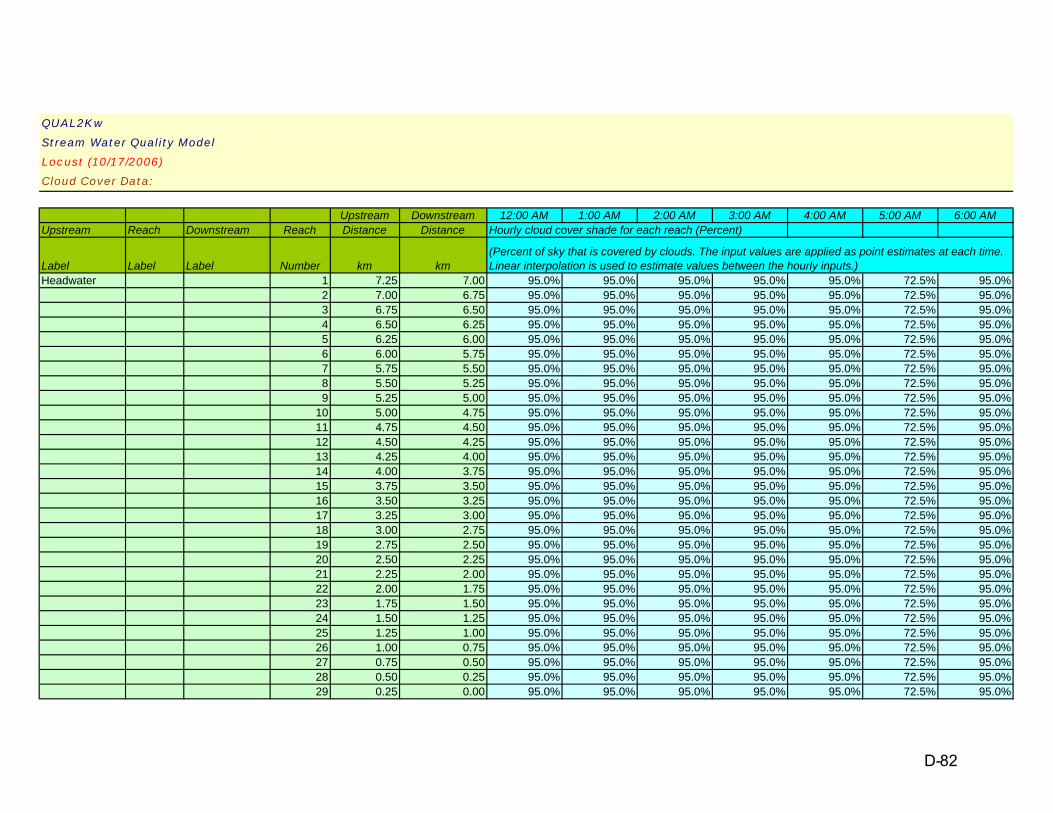
QUAL2Kw
Stream Water Quality Model
Locust (10/17/2006)
Cloud Cover Data:
Upstream Downstream 12:00 AM 1:00 AM 2:00 AM 3:00 AM 4:00 AM 5:00 AM 6:00 AMUpstream Reach Downstream Reach Distance Distance Hourly cloud cover shade for each reach (Percent)
Label Label Label Number km kmHeadwater 1 7.25 7.00 95.0% 95.0% 95.0% 95.0% 95.0% 72.5% 95.0%
2 7.00 6.75 95.0% 95.0% 95.0% 95.0% 95.0% 72.5% 95.0%3 6.75 6.50 95.0% 95.0% 95.0% 95.0% 95.0% 72.5% 95.0%4 6.50 6.25 95.0% 95.0% 95.0% 95.0% 95.0% 72.5% 95.0%5 6.25 6.00 95.0% 95.0% 95.0% 95.0% 95.0% 72.5% 95.0%6 6.00 5.75 95.0% 95.0% 95.0% 95.0% 95.0% 72.5% 95.0%7 5.75 5.50 95.0% 95.0% 95.0% 95.0% 95.0% 72.5% 95.0%8 5.50 5.25 95.0% 95.0% 95.0% 95.0% 95.0% 72.5% 95.0%9 5.25 5.00 95.0% 95.0% 95.0% 95.0% 95.0% 72.5% 95.0%
10 5.00 4.75 95.0% 95.0% 95.0% 95.0% 95.0% 72.5% 95.0%11 4.75 4.50 95.0% 95.0% 95.0% 95.0% 95.0% 72.5% 95.0%12 4.50 4.25 95.0% 95.0% 95.0% 95.0% 95.0% 72.5% 95.0%13 4.25 4.00 95.0% 95.0% 95.0% 95.0% 95.0% 72.5% 95.0%14 4.00 3.75 95.0% 95.0% 95.0% 95.0% 95.0% 72.5% 95.0%15 3.75 3.50 95.0% 95.0% 95.0% 95.0% 95.0% 72.5% 95.0%16 3.50 3.25 95.0% 95.0% 95.0% 95.0% 95.0% 72.5% 95.0%17 3.25 3.00 95.0% 95.0% 95.0% 95.0% 95.0% 72.5% 95.0%18 3.00 2.75 95.0% 95.0% 95.0% 95.0% 95.0% 72.5% 95.0%19 2.75 2.50 95.0% 95.0% 95.0% 95.0% 95.0% 72.5% 95.0%20 2.50 2.25 95.0% 95.0% 95.0% 95.0% 95.0% 72.5% 95.0%21 2.25 2.00 95.0% 95.0% 95.0% 95.0% 95.0% 72.5% 95.0%22 2.00 1.75 95.0% 95.0% 95.0% 95.0% 95.0% 72.5% 95.0%23 1.75 1.50 95.0% 95.0% 95.0% 95.0% 95.0% 72.5% 95.0%24 1.50 1.25 95.0% 95.0% 95.0% 95.0% 95.0% 72.5% 95.0%25 1.25 1.00 95.0% 95.0% 95.0% 95.0% 95.0% 72.5% 95.0%26 1.00 0.75 95.0% 95.0% 95.0% 95.0% 95.0% 72.5% 95.0%27 0.75 0.50 95.0% 95.0% 95.0% 95.0% 95.0% 72.5% 95.0%28 0.50 0.25 95.0% 95.0% 95.0% 95.0% 95.0% 72.5% 95.0%29 0.25 0.00 95.0% 95.0% 95.0% 95.0% 95.0% 72.5% 95.0%
(Percent of sky that is covered by clouds. The input values are applied as point estimates at each time. Linear interpolation is used to estimate values between the hourly inputs.)
D-82

Reach
Number123456789
1011121314151617181920212223242526272829
QUAL2Kw
Stream Water Quality Model
Locust (10/17/2006)
Cloud Cover Data:
7:00 AM 8:00 AM 9:00 AM 10:00 AM 11:00 AM 12:00 PM 1:00 PM 2:00 PM 3:00 PM
95.0% 95.0% 95.0% 95.0% 95.0% 91.3% 95.0% 95.0% 95.0%95.0% 95.0% 95.0% 95.0% 95.0% 91.3% 95.0% 95.0% 95.0%95.0% 95.0% 95.0% 95.0% 95.0% 91.3% 95.0% 95.0% 95.0%95.0% 95.0% 95.0% 95.0% 95.0% 91.3% 95.0% 95.0% 95.0%95.0% 95.0% 95.0% 95.0% 95.0% 91.3% 95.0% 95.0% 95.0%95.0% 95.0% 95.0% 95.0% 95.0% 91.3% 95.0% 95.0% 95.0%95.0% 95.0% 95.0% 95.0% 95.0% 91.3% 95.0% 95.0% 95.0%95.0% 95.0% 95.0% 95.0% 95.0% 91.3% 95.0% 95.0% 95.0%95.0% 95.0% 95.0% 95.0% 95.0% 91.3% 95.0% 95.0% 95.0%95.0% 95.0% 95.0% 95.0% 95.0% 91.3% 95.0% 95.0% 95.0%95.0% 95.0% 95.0% 95.0% 95.0% 91.3% 95.0% 95.0% 95.0%95.0% 95.0% 95.0% 95.0% 95.0% 91.3% 95.0% 95.0% 95.0%95.0% 95.0% 95.0% 95.0% 95.0% 91.3% 95.0% 95.0% 95.0%95.0% 95.0% 95.0% 95.0% 95.0% 91.3% 95.0% 95.0% 95.0%95.0% 95.0% 95.0% 95.0% 95.0% 91.3% 95.0% 95.0% 95.0%95.0% 95.0% 95.0% 95.0% 95.0% 91.3% 95.0% 95.0% 95.0%95.0% 95.0% 95.0% 95.0% 95.0% 91.3% 95.0% 95.0% 95.0%95.0% 95.0% 95.0% 95.0% 95.0% 91.3% 95.0% 95.0% 95.0%95.0% 95.0% 95.0% 95.0% 95.0% 91.3% 95.0% 95.0% 95.0%95.0% 95.0% 95.0% 95.0% 95.0% 91.3% 95.0% 95.0% 95.0%95.0% 95.0% 95.0% 95.0% 95.0% 91.3% 95.0% 95.0% 95.0%95.0% 95.0% 95.0% 95.0% 95.0% 91.3% 95.0% 95.0% 95.0%95.0% 95.0% 95.0% 95.0% 95.0% 91.3% 95.0% 95.0% 95.0%95.0% 95.0% 95.0% 95.0% 95.0% 91.3% 95.0% 95.0% 95.0%95.0% 95.0% 95.0% 95.0% 95.0% 91.3% 95.0% 95.0% 95.0%95.0% 95.0% 95.0% 95.0% 95.0% 91.3% 95.0% 95.0% 95.0%95.0% 95.0% 95.0% 95.0% 95.0% 91.3% 95.0% 95.0% 95.0%95.0% 95.0% 95.0% 95.0% 95.0% 91.3% 95.0% 95.0% 95.0%95.0% 95.0% 95.0% 95.0% 95.0% 91.3% 95.0% 95.0% 95.0%
D-83

Reach
Number123456789
1011121314151617181920212223242526272829
QUAL2Kw
Stream Water Quality Model
Locust (10/17/2006)
Cloud Cover Data:
4:00 PM 5:00 PM 6:00 PM 7:00 PM 8:00 PM 9:00 PM 10:00 PM 11:00 PM
95.0% 95.0% 95.0% 95.0% 95.0% 95.0% 95.0% 95.0%95.0% 95.0% 95.0% 95.0% 95.0% 95.0% 95.0% 95.0%95.0% 95.0% 95.0% 95.0% 95.0% 95.0% 95.0% 95.0%95.0% 95.0% 95.0% 95.0% 95.0% 95.0% 95.0% 95.0%95.0% 95.0% 95.0% 95.0% 95.0% 95.0% 95.0% 95.0%95.0% 95.0% 95.0% 95.0% 95.0% 95.0% 95.0% 95.0%95.0% 95.0% 95.0% 95.0% 95.0% 95.0% 95.0% 95.0%95.0% 95.0% 95.0% 95.0% 95.0% 95.0% 95.0% 95.0%95.0% 95.0% 95.0% 95.0% 95.0% 95.0% 95.0% 95.0%95.0% 95.0% 95.0% 95.0% 95.0% 95.0% 95.0% 95.0%95.0% 95.0% 95.0% 95.0% 95.0% 95.0% 95.0% 95.0%95.0% 95.0% 95.0% 95.0% 95.0% 95.0% 95.0% 95.0%95.0% 95.0% 95.0% 95.0% 95.0% 95.0% 95.0% 95.0%95.0% 95.0% 95.0% 95.0% 95.0% 95.0% 95.0% 95.0%95.0% 95.0% 95.0% 95.0% 95.0% 95.0% 95.0% 95.0%95.0% 95.0% 95.0% 95.0% 95.0% 95.0% 95.0% 95.0%95.0% 95.0% 95.0% 95.0% 95.0% 95.0% 95.0% 95.0%95.0% 95.0% 95.0% 95.0% 95.0% 95.0% 95.0% 95.0%95.0% 95.0% 95.0% 95.0% 95.0% 95.0% 95.0% 95.0%95.0% 95.0% 95.0% 95.0% 95.0% 95.0% 95.0% 95.0%95.0% 95.0% 95.0% 95.0% 95.0% 95.0% 95.0% 95.0%95.0% 95.0% 95.0% 95.0% 95.0% 95.0% 95.0% 95.0%95.0% 95.0% 95.0% 95.0% 95.0% 95.0% 95.0% 95.0%95.0% 95.0% 95.0% 95.0% 95.0% 95.0% 95.0% 95.0%95.0% 95.0% 95.0% 95.0% 95.0% 95.0% 95.0% 95.0%95.0% 95.0% 95.0% 95.0% 95.0% 95.0% 95.0% 95.0%95.0% 95.0% 95.0% 95.0% 95.0% 95.0% 95.0% 95.0%95.0% 95.0% 95.0% 95.0% 95.0% 95.0% 95.0% 95.0%95.0% 95.0% 95.0% 95.0% 95.0% 95.0% 95.0% 95.0%
D-84

QUAL2Kw
Stream Water Quality Model
Locust (10/17/2006)
Shade Data:
Upstream Downstream 12:00 AM 1:00 AM 2:00 AM 3:00 AM 4:00 AM 5:00 AMUpstream Reach Downstream Reach Distance Distance Integrated hourly effective shade for each reach (Percent)
Label Label Label Number km kmHeadwater 1 7.25 7.00 15.0% 15.0% 15.0% 15.0% 15.0% 15.0%
2 7.00 6.75 15.0% 15.0% 15.0% 15.0% 15.0% 15.0%3 6.75 6.50 15.0% 15.0% 15.0% 15.0% 15.0% 15.0%4 6.50 6.25 15.0% 15.0% 15.0% 15.0% 15.0% 15.0%5 6.25 6.00 15.0% 15.0% 15.0% 15.0% 15.0% 15.0%6 6.00 5.75 15.0% 15.0% 15.0% 15.0% 15.0% 15.0%7 5.75 5.50 15.0% 15.0% 15.0% 15.0% 15.0% 15.0%8 5.50 5.25 15.0% 15.0% 15.0% 15.0% 15.0% 15.0%9 5.25 5.00 15.0% 15.0% 15.0% 15.0% 15.0% 15.0%
10 5.00 4.75 15.0% 15.0% 15.0% 15.0% 15.0% 15.0%11 4.75 4.50 15.0% 15.0% 15.0% 15.0% 15.0% 15.0%12 4.50 4.25 15.0% 15.0% 15.0% 15.0% 15.0% 15.0%13 4.25 4.00 15.0% 15.0% 15.0% 15.0% 15.0% 15.0%14 4.00 3.75 15.0% 15.0% 15.0% 15.0% 15.0% 15.0%15 3.75 3.50 15.0% 15.0% 15.0% 15.0% 15.0% 15.0%16 3.50 3.25 15.0% 15.0% 15.0% 15.0% 15.0% 15.0%17 3.25 3.00 15.0% 15.0% 15.0% 15.0% 15.0% 15.0%18 3.00 2.75 15.0% 15.0% 15.0% 15.0% 15.0% 15.0%19 2.75 2.50 15.0% 15.0% 15.0% 15.0% 15.0% 15.0%20 2.50 2.25 15.0% 15.0% 15.0% 15.0% 15.0% 15.0%21 2.25 2.00 15.0% 15.0% 15.0% 15.0% 15.0% 15.0%22 2.00 1.75 15.0% 15.0% 15.0% 15.0% 15.0% 15.0%23 1.75 1.50 15.0% 15.0% 15.0% 15.0% 15.0% 15.0%24 1.50 1.25 15.0% 15.0% 15.0% 15.0% 15.0% 15.0%25 1.25 1.00 15.0% 15.0% 15.0% 15.0% 15.0% 15.0%26 1.00 0.75 15.0% 15.0% 15.0% 15.0% 15.0% 15.0%27 0.75 0.50 15.0% 15.0% 15.0% 15.0% 15.0% 15.0%28 0.50 0.25 15.0% 15.0% 15.0% 15.0% 15.0% 15.0%29 0.25 0.00 15.0% 15.0% 15.0% 15.0% 15.0% 15.0%
(Percent of solar radiation that is blocked because of shade from topography and vegetation. Hourly values are applied as integrated values for each hour, e.g. the value at 12:00 AM is applied from 12:00 to 1:00 AM)
D-85

Reach
Number123456789
1011121314151617181920212223242526272829
QUAL2Kw
Stream Water Quality Model
Locust (10/17/2006)
Shade Data:
6:00 AM 7:00 AM 8:00 AM 9:00 AM 10:00 AM 11:00 AM 12:00 PM 1:00 PM 2:00 PM 3:00 PM
15.0% 15.0% 15.0% 15.0% 15.0% 15.0% 15.0% 15.0% 15.0% 15.0%15.0% 15.0% 15.0% 15.0% 15.0% 15.0% 15.0% 15.0% 15.0% 15.0%15.0% 15.0% 15.0% 15.0% 15.0% 15.0% 15.0% 15.0% 15.0% 15.0%15.0% 15.0% 15.0% 15.0% 15.0% 15.0% 15.0% 15.0% 15.0% 15.0%15.0% 15.0% 15.0% 15.0% 15.0% 15.0% 15.0% 15.0% 15.0% 15.0%15.0% 15.0% 15.0% 15.0% 15.0% 15.0% 15.0% 15.0% 15.0% 15.0%15.0% 15.0% 15.0% 15.0% 15.0% 15.0% 15.0% 15.0% 15.0% 15.0%15.0% 15.0% 15.0% 15.0% 15.0% 15.0% 15.0% 15.0% 15.0% 15.0%15.0% 15.0% 15.0% 15.0% 15.0% 15.0% 15.0% 15.0% 15.0% 15.0%15.0% 15.0% 15.0% 15.0% 15.0% 15.0% 15.0% 15.0% 15.0% 15.0%15.0% 15.0% 15.0% 15.0% 15.0% 15.0% 15.0% 15.0% 15.0% 15.0%15.0% 15.0% 15.0% 15.0% 15.0% 15.0% 15.0% 15.0% 15.0% 15.0%15.0% 15.0% 15.0% 15.0% 15.0% 15.0% 15.0% 15.0% 15.0% 15.0%15.0% 15.0% 15.0% 15.0% 15.0% 15.0% 15.0% 15.0% 15.0% 15.0%15.0% 15.0% 15.0% 15.0% 15.0% 15.0% 15.0% 15.0% 15.0% 15.0%15.0% 15.0% 15.0% 15.0% 15.0% 15.0% 15.0% 15.0% 15.0% 15.0%15.0% 15.0% 15.0% 15.0% 15.0% 15.0% 15.0% 15.0% 15.0% 15.0%15.0% 15.0% 15.0% 15.0% 15.0% 15.0% 15.0% 15.0% 15.0% 15.0%15.0% 15.0% 15.0% 15.0% 15.0% 15.0% 15.0% 15.0% 15.0% 15.0%15.0% 15.0% 15.0% 15.0% 15.0% 15.0% 15.0% 15.0% 15.0% 15.0%15.0% 15.0% 15.0% 15.0% 15.0% 15.0% 15.0% 15.0% 15.0% 15.0%15.0% 15.0% 15.0% 15.0% 15.0% 15.0% 15.0% 15.0% 15.0% 15.0%15.0% 15.0% 15.0% 15.0% 15.0% 15.0% 15.0% 15.0% 15.0% 15.0%15.0% 15.0% 15.0% 15.0% 15.0% 15.0% 15.0% 15.0% 15.0% 15.0%15.0% 15.0% 15.0% 15.0% 15.0% 15.0% 15.0% 15.0% 15.0% 15.0%15.0% 15.0% 15.0% 15.0% 15.0% 15.0% 15.0% 15.0% 15.0% 15.0%15.0% 15.0% 15.0% 15.0% 15.0% 15.0% 15.0% 15.0% 15.0% 15.0%15.0% 15.0% 15.0% 15.0% 15.0% 15.0% 15.0% 15.0% 15.0% 15.0%15.0% 15.0% 15.0% 15.0% 15.0% 15.0% 15.0% 15.0% 15.0% 15.0%
D-86

Reach
Number123456789
1011121314151617181920212223242526272829
QUAL2Kw
Stream Water Quality Model
Locust (10/17/2006)
Shade Data:
4:00 PM 5:00 PM 6:00 PM 7:00 PM 8:00 PM 9:00 PM 10:00 PM 11:00 PM
15.0% 15.0% 15.0% 15.0% 15.0% 15.0% 15.0% 15.0%15.0% 15.0% 15.0% 15.0% 15.0% 15.0% 15.0% 15.0%15.0% 15.0% 15.0% 15.0% 15.0% 15.0% 15.0% 15.0%15.0% 15.0% 15.0% 15.0% 15.0% 15.0% 15.0% 15.0%15.0% 15.0% 15.0% 15.0% 15.0% 15.0% 15.0% 15.0%15.0% 15.0% 15.0% 15.0% 15.0% 15.0% 15.0% 15.0%15.0% 15.0% 15.0% 15.0% 15.0% 15.0% 15.0% 15.0%15.0% 15.0% 15.0% 15.0% 15.0% 15.0% 15.0% 15.0%15.0% 15.0% 15.0% 15.0% 15.0% 15.0% 15.0% 15.0%15.0% 15.0% 15.0% 15.0% 15.0% 15.0% 15.0% 15.0%15.0% 15.0% 15.0% 15.0% 15.0% 15.0% 15.0% 15.0%15.0% 15.0% 15.0% 15.0% 15.0% 15.0% 15.0% 15.0%15.0% 15.0% 15.0% 15.0% 15.0% 15.0% 15.0% 15.0%15.0% 15.0% 15.0% 15.0% 15.0% 15.0% 15.0% 15.0%15.0% 15.0% 15.0% 15.0% 15.0% 15.0% 15.0% 15.0%15.0% 15.0% 15.0% 15.0% 15.0% 15.0% 15.0% 15.0%15.0% 15.0% 15.0% 15.0% 15.0% 15.0% 15.0% 15.0%15.0% 15.0% 15.0% 15.0% 15.0% 15.0% 15.0% 15.0%15.0% 15.0% 15.0% 15.0% 15.0% 15.0% 15.0% 15.0%15.0% 15.0% 15.0% 15.0% 15.0% 15.0% 15.0% 15.0%15.0% 15.0% 15.0% 15.0% 15.0% 15.0% 15.0% 15.0%15.0% 15.0% 15.0% 15.0% 15.0% 15.0% 15.0% 15.0%15.0% 15.0% 15.0% 15.0% 15.0% 15.0% 15.0% 15.0%15.0% 15.0% 15.0% 15.0% 15.0% 15.0% 15.0% 15.0%15.0% 15.0% 15.0% 15.0% 15.0% 15.0% 15.0% 15.0%15.0% 15.0% 15.0% 15.0% 15.0% 15.0% 15.0% 15.0%15.0% 15.0% 15.0% 15.0% 15.0% 15.0% 15.0% 15.0%15.0% 15.0% 15.0% 15.0% 15.0% 15.0% 15.0% 15.0%15.0% 15.0% 15.0% 15.0% 15.0% 15.0% 15.0% 15.0%
D-87

QUAL2Kw
Stream Water Quality Model
Locust (10/17/2006)
Light Parameters and Surface Heat Transfer Models:
Parameter Value UnitPhotosynthetically Available Radiation 0.47Background light extinction 0.2 /m k eb
Linear chlorophyll light extinction 0.0088 1/m-(ugA/L) α p
Nonlinear chlorophyll light extinction 0.054 1/m-(ugA/L) 2/3 α pn
ISS light extinction 0.052 1/m-(mgD/L) α ι
Detritus light extinction 0.174 1/m-(mgD/L) α ο
Macrophyte light extinction 0.015 1/m-(gD/m 3 ) α macSolar shortwave radiation modelAtmospheric attenuation model for solar BrasBras solar parameter (used if Bras solar model is selected)atmospheric turbidity coefficient (2=clear, 5=smoggy, default=2) 3 n fac
Ryan-Stolzenbach solar parameter (used if Ryan-Stolzenbach solar model is selected)atmospheric transmission coefficient (0.70-0.91, default 0.8) 0.8 a tc
Downwelling atmospheric longwave IR radiationatmospheric longwave emissivity model BruntEvaporation and air convection/conductionwind speed function for evaporation and air convection/conduction Brady-Graves-Geyer
D-88

QUAL2Kw
Stream Water Quality Model
Locust (10/17/2006)
Diffuse Source Data:
Diffuse Diffuse Spec Inorg Diss CBOD CBOD OrganicAbstraction Inflow Temp Cond SS Oxygen slow fast N
Name Up (km) Down (km) m3/s m3/s C umhos mgD/L mg/L mgO2/L mgO2/L ugN/L1.00 7.2500 3.2900 0.00 0.02 14.00 0.00 0.00 4.00 55.0 27.0 1500.01.00 3.2900 0.0000 0.01 14.00 0.00 0.00 4.00 55.0 27.0 1500.0
D-89
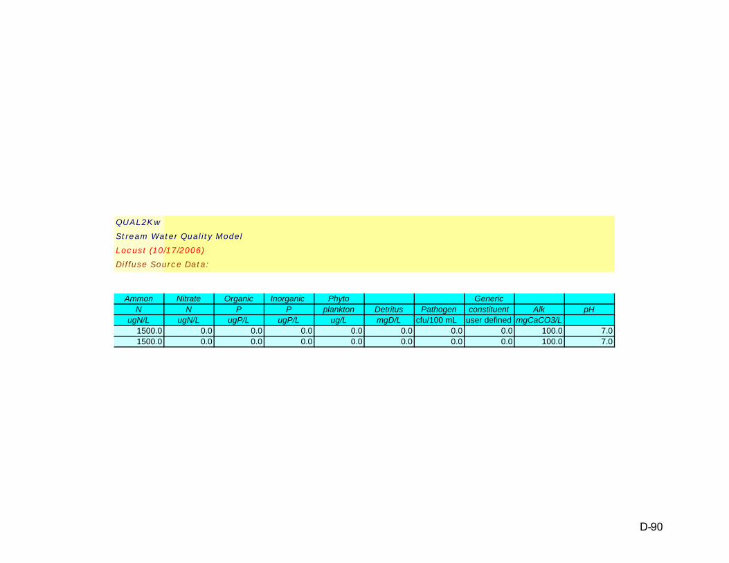
QUAL2Kw
Stream Water Quality Model
Locust (10/17/2006)
Diffuse Source Data:
Ammon Nitrate Organic Inorganic Phyto GenericN N P P plankton Detritus Pathogen constituent Alk pH
ugN/L ugN/L ugP/L ugP/L ug/L mgD/L cfu/100 mL user defined mgCaCO3/L1500.0 0.0 0.0 0.0 0.0 0.0 0.0 0.0 100.0 7.01500.0 0.0 0.0 0.0 0.0 0.0 0.0 0.0 100.0 7.0
D-90

QUAL2Kw
Stream Water Quality Model Fitness:
Locust (10/17/2006) 1.85658
Global rate parameters
Parameter Value Units Symbol Auto-cal Min value Max valueStoichiometry:Carbon 40 gC gC No 30 50Nitrogen 7.2 gN gN No 3 9Phosphorus 1 gP gP No 0.4 2Dry weight 100 gD gD No 100 100Chlorophyll 1 gA gA No 0.4 2Inorganic suspended solids:Settling velocity 0.00236 m/d v i Yes 0 2Oxygen:Reaeration model O'Connor-Dobbins f(u h)Temp correction 1.024 θ a
Reaeration wind effect NoneO2 for carbon oxidation 2.69 gO2/gC r oc
O2 for NH4 nitrification 4.57 gO2/gN r on
Oxygen inhib model CBOD oxidation ExponentialOxygen inhib parameter CBOD oxidation 0.60 L/mgO2 K socf No 0.60 0.60Oxygen inhib model nitrification ExponentialOxygen inhib parameter nitrification 0.60 L/mgO2 K sona No 0.60 0.60Oxygen enhance model denitrification ExponentialOxygen enhance parameter denitrification 0.60 L/mgO2 K sodn No 0.60 0.60Oxygen inhib model phyto resp ExponentialOxygen inhib parameter phyto resp 0.60 L/mgO2 K sop No 0.60 0.60Oxygen enhance model bot alg resp ExponentialOxygen enhance parameter bot alg resp 0.60 L/mgO2 K sob No 0.60 0.60Slow CBOD:Hydrolysis rate 0.5 /d k hc Yes 0 5Temp correction 1.047 θ hc No 1 1.07Oxidation rate 0.1 /d k dcs Yes 0 5Temp correction 1.047 θ dcs No 1 1.07Fast CBOD:Oxidation rate 3.4 /d k dc Yes 0 5Temp correction 1.047 θ dc No 1 1.07Organic N:Hydrolysis 0.5 /d k hn Yes 0 5Temp correction 1.07 θ hn No 1 1.07Settling velocity 0.1 m/d v on Yes 0 2Ammonium:
Auto-calibration inputs
D-91

QUAL2Kw
Stream Water Quality Model Fitness:
Locust (10/17/2006) 1.85658
Global rate parameters
Parameter Value Units Symbol Auto-cal Min value Max valueAuto-calibration inputs
Nitrification 1 /d k na Yes 0 10Temp correction 1.07 θ na No 1 1.07Nitrate:Denitrification 0.01 /d k dn Yes 0 2Temp correction 1.07 θ dn No 1 1.07Sed denitrification transfer coeff 0.01 m/d v di Yes 0 1Temp correction 1.07 θ di No 1 1.07Organic P:Hydrolysis 0 /d k hp Yes 0 5Temp correction 1.07 θ hp No 1 1.07Settling velocity 0.84512 m/d v op Yes 0 2Inorganic P:Settling velocity 0 m/d v ip Yes 0 2Sed P oxygen attenuation half sat constant 0.65786 mgO2/L k spi Yes 0 2Phytoplankton:Max Growth rate 0 /d k gp No 1.5 3Temp correction 1.07 θ gp No 1 1.07Respiration rate 0 /d k rp No 0 1Temp correction 1.07 θ rp No 1 1.07Death rate 0 /d k dp No 0 1Temp correction 1 θ dp No 1 1.07Nitrogen half sat constant 15 ugN/L k sPp No 0 150Phosphorus half sat constant 2 ugP/L k sNp No 0 50Inorganic carbon half sat constant 1.30E-05 moles/L k sCp No 1.30E-06 1.30E-04Phytoplankton use HCO3- as substrate YesLight model Half saturationLight constant 57.6 langleys/d K Lp No 28.8 115.2Ammonia preference 25 ugN/L k hnxp No 25 25Settling velocity 0.15 m/d v a No 0 5Bottom Plants:
Growth model Zero-order
Max Growth rate 0 mgA/m2/d or /d C gb Yes 0 500
Temp correction 1.07 θ gb No 1 1.07
First-order model carrying capacity 1000 mgA/m2 a b,max No 1000 1000
Respiration rate 0 /d k rb Yes 0 0.5
Temp correction 1.07 θ rb No 1 1.07
D-92

QUAL2Kw
Stream Water Quality Model Fitness:
Locust (10/17/2006) 1.85658
Global rate parameters
Parameter Value Units Symbol Auto-cal Min value Max valueAuto-calibration inputs
Excretion rate 0 /d k eb Yes 0 0.5
Temp correction 1.07 θ db No 1 1.07
Death rate 0 /d k db Yes 0 0.5
Temp correction 1.07 θ db No 1 1.07
External nitrogen half sat constant 103.596 ugN/L k sPb Yes 0 300
External phosphorus half sat constant 79.313 ugP/L k sNb Yes 0 100
Inorganic carbon half sat constant 2.50E-06 moles/L k sCb Yes 1.30E-06 1.30E-04
Bottom algae use HCO3- as substrate Yes
Light model Half saturation
Light constant 3.58588 langleys/d K Lb Yes 1 100
Ammonia preference 22.48993 ugN/L k hnxb Yes 1 100
Subsistence quota for nitrogen 0.63189468 mgN/mgA q 0N Yes 0.0072 7.2
Subsistence quota for phosphorus 0.03389707 mgP/mgA q 0P Yes 0.001 1
Maximum uptake rate for nitrogen 72.64143 mgN/mgA/d ρ mN Yes 35 150
Maximum uptake rate for phosphorus 15.03188 mgP/mgA/d ρ mP Yes 5 20
Internal nitrogen half sat ratio 3.9246125 K qN,ratio Yes 1.05 5
Internal phosphorus half sat ratio 1.3342815 K qP,ratio Yes 1.05 5
Nitrogen uptake water column fraction 1 N UpWCfrac No 0 1
Phosphorus uptake water column fraction 1 P UpWCfrac No 0 1Detritus (POM):Dissolution rate 0 /d k dt Yes 0 5Temp correction 1.07 θ dt No 1.07 1.07Settling velocity 0 m/d v dt Yes 0 5Pathogens:Decay rate 0 /d k dx No 0.8 0.8Temp correction 1.07 θ dx No 1.07 1.07Settling velocity 1 m/d v x No 1 1alpha constant for light mortality 1 /d per ly/hr apath No 1 1pH:Partial pressure of carbon dioxide 347 ppm p CO2
Hyporheic metabolismModel for biofilm oxidation of fast CBOD Zero-order level 1Max biofilm growth rate 5 gO2/m^2/d or /d " No 0 20
D-93

QUAL2Kw
Stream Water Quality Model Fitness:
Locust (10/17/2006) 1.85658
Global rate parameters
Parameter Value Units Symbol Auto-cal Min value Max valueAuto-calibration inputs
Temp correction 1.047 " No 1.047 1.047Fast CBOD half-saturation 0.5 mgO2/L " No 0 2Oxygen inhib model Exponential "Oxygen inhib parameter 0.60 L/mgO2 " No 0.60 0.60Respiration rate 0.2 /d level 2 No 0.2 0.2Temp correction 1.07 " No 1.07 1.07Death rate 0.05 /d " No 0.05 0.05Temp correction 1.07 " No 1.07 1.07External nitrogen half sat constant 15 ugN/L " No 15 15External phosphorus half sat constant 2 ugP/L " No 2 2Ammonia preference 25 ugN/L " No 25 25First-order model carrying capacity 100 gD/m2 " No 100 100Generic constituentDecay rate 0.8 /d No 0.8 0.8Temp correction 1.07 No 1.07 1.07Settling velocity 1 m/d No 1 1Use generic constituent as COD? NoUser-defined auto-calibration parameters (optional)Point source pH at location 10.2 Km 7.43916 6 7.5
D-94

QUAL2Kw
Stream Water Quality Model
Locust (10/17/2006)
Global rate parameters
Random number seed 123456 seedModel runs in a population (<=512) 4 npGenerations in the evolution 2 ngenDigits to encode genotype (<=6) 5 ndCrossover mode (1, 2, 3, 4, 5, 6, or 7) 3 icrossCrossover probability (0-1): 0.85 pcrossMutation mode (1, 2, 3, 4, 5, or 6) 2 imutInitial mutation rate (0-1): 0.005 pmutMinimum mutation rate (0-1): 0.0005 pmutmnMaximum mutation rate (0-1): 0.25 pmutmxRelative fitness differential (0-1): 1 fdifReproduction plan (1, 2, or 3): 1 irepElitism (0 or 1): 1 ieliteRestart from previous evolution (0 or 1): 0 irestart
Auto-calibration genetic algorithm control:
D-95

Locust (10/17/2006)
0.00
0.01
0.01
0.02
0.02
0.03
0.03
0.04
0.04
0.05
01234567distance upstream (Km)
flow
(m^3
/s)
Q, m3/s Q-data m3/s
D-96
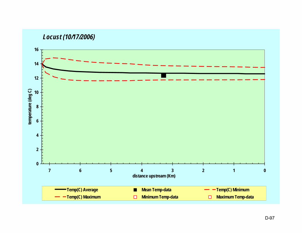
Locust (10/17/2006)
0
2
4
6
8
10
12
14
16
01234567distance upstream (Km)
tem
pera
ture
(deg
C)
Temp(C) Average Mean Temp-data Temp(C) MinimumTemp(C) Maximum Minimum Temp-data Maximum Temp-data
D-97

Locust (10/17/2006)
0
2
4
6
8
10
12
01234567distance upstream (Km)
diss
olve
d ox
ygen
(mg/
L)
DO(mgO2/L) DO (mgO2/L) data DO(mgO2/L) Min DO(mgO2/L) MaxMinimum DO-data Maximum DO-data DO sat
D-98
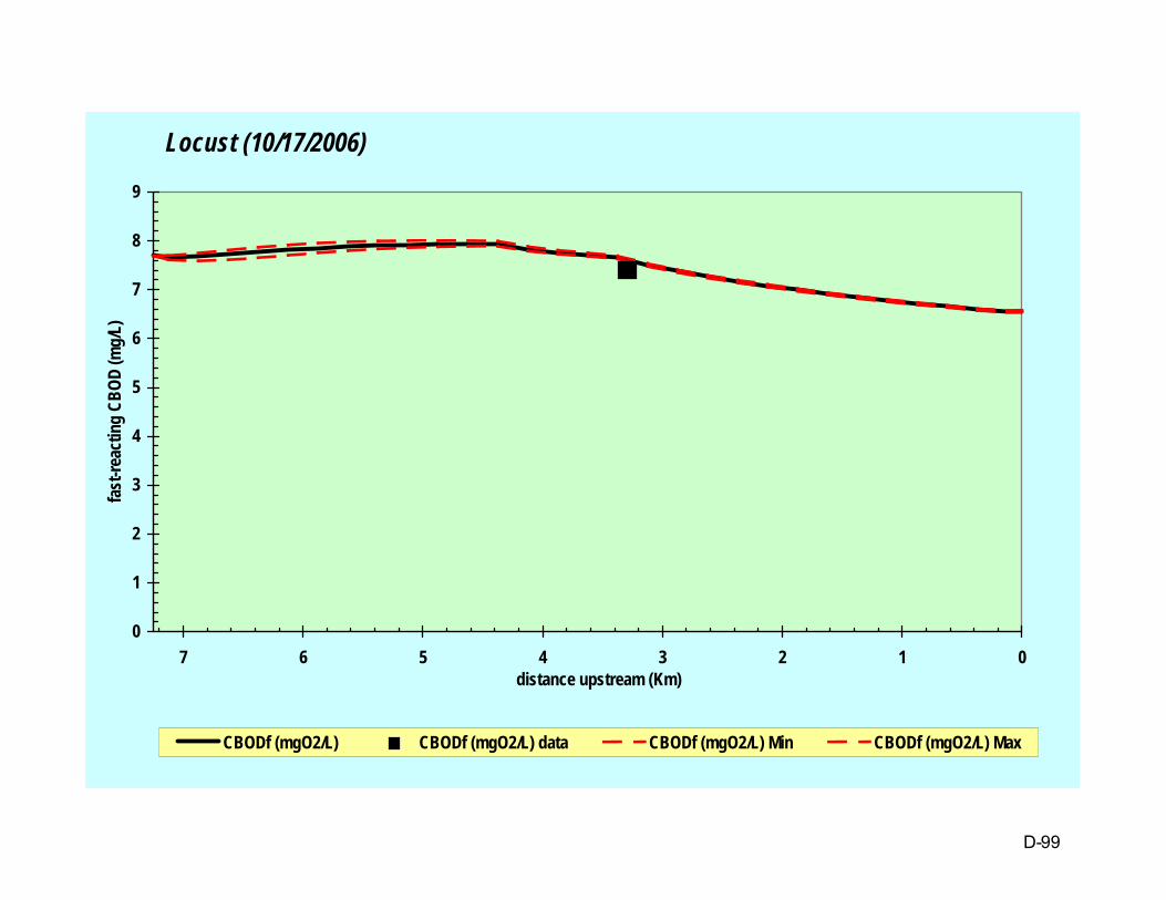
Locust (10/17/2006)
0
1
2
3
4
5
6
7
8
9
01234567distance upstream (Km)
fast
-reac
ting
CBOD
(mg/
L)
CBODf (mgO2/L) CBODf (mgO2/L) data CBODf (mgO2/L) Min CBODf (mgO2/L) Max
D-99

Illinois Environmental Protection Agency TMDL Development for the Shoal Creek Watershed
Final Report for USEPA Approval E-1
Appendix E : Stage 1 Report

Illinois Environmental Protection Agency TMDL Development for the Shoal Creek Watershed
Final Report for USEPA Approval F-1
Appendix F : Stage 2 Report

Illinois Environmental Protection Agency TMDL Development for the Shoal Creek Watershed
Final Report for USEPA Approval F-2

Illinois Environmental Protection Agency TMDL Development for the Shoal Creek Watershed
Final Report for USEPA Approval G-1
Appendix G : Responsiveness Summary

Illinois Environmental Protection Agency TMDL Development for the Shoal Creek Watershed
Final Report for USEPA Approval G-2
This responsiveness summary responds to substantive questions and comments received during the public comment period from July 31, 2007 through August 17, 2007 postmarked, including those from the August 6, 2007 public meeting discussed below.
What is a TMDL?
A Total Maximum Daily Load (TMDL) is the sum of the allowable amount of a pollutant that a water body can receive from all contributing sources and still meet water quality standards or designated uses. This TMDL is for the Shoal Creek watershed. This report details the watershed characteristics, impairment, sources, load and wasteload allocations, and reductions for each segment. The Illinois EPA implements the TMDL program in accordance with Section 303(d) of the federal Clean Water Act and regulations there under.
Background
The portion of the Shoal Creek watershed addressed in this report has a drainage area of approximately 310 square miles This watershed is part of Bond, Montgomery, Clinton and Madison counties. Land use in the is 72 percent agriculture, 16 percent forest, nine percent urban and two percent urban. Waters impaired in this watershed are Shoal Creek, Locust Fork, Chicken Creek and Cattle Creek. Shoal Creek is listed on the Illinois EPA 2006 Section 303(d) List as being impaired for public water supply use with the potential cause of manganese. It is also impaired for primary contact recreation (swimming) use with the potential cause of fecal coliform. Locust Fork is impaired for aquatic life use with the potential cause of low dissolved oxygen. Chicken Creek is impaired for aquatic life use with the potential causes of low dissolved oxygen and silver. Cattle Creek is impaired for aquatic life use with the potential causes of ammonia, copper, low dissolved oxygen and total dissolved solids. The Clean Water Act and USEPA regulations require that states develop TMDLs for waters on the Section 303(d) List. 6.0 PUBLIC MEETINGS Public meetings were held in Sorento on June 28, 2006, August 6, 2007 and April 10, 2008. The Illinois EPA provided public notices for all meetings by placing display ads in three newspapers in the watershed; the Sorento News, Greenville Advocate and the Breese Journal. These notices gave the date, time, location, and purpose of the meetings. It also provided references to obtain additional information about this specific site, the TMDL Program and other related issues. Individuals and organizations were also sent the public notice by first class mail. The draft TMDL Report was available for review at the Sorento Village Hall, Breese City Hall and also on the Agency’s web page at http://www.epa.state.il.us/water/tmdl . The first public meeting on June 28, 2006 started at 6:00 p.m. and was attended by approximately seven people. The second public meeting on August 6, 2007, started at 6:00 p.m. and was attended by nine people. The meeting record remained open until midnight, August 17, 2007. The third public meeting for the implementation plan was held on April 10, 2008 and was attended by nine people.

Illinois Environmental Protection Agency TMDL Development for the Shoal Creek Watershed
Final Report for USEPA Approval G-3
Questions and Comments
1. Where does fecal coliform come from?
Response Fecal coliform are bacteria in wastes from warm-blooded mammals. It is used as an “indicator organism” because excessive amounts in surface water have been known to indicate increased risk of pathogen-induced illness to humans. Infection due to pathogen-contaminated recreational waters can include gastrointestinal, respiratory, eye, and skin diseases. Fecal coliform sources are humans and animals.
2. Are sewage treatment plants allowed to discharge fecal coliform?
Response Some plants have limits for fecal coliform in their discharge. This limit is given to sewage treatment plants in their NPDES permit and they must monitor to show compliance. Some treatment plants have been given a chlorination exemption in which they do not chlorinate or monitor for fecal coliform. In order to attain this, the plant must prove there is no primary contact (swimming) in the water it is discharging into and submit data to show that at the end of the water reach, the fecal count is lower than 200 cfu/100ml.
3. Does anyone use ozone for disinfection?
Response No facility in Illinois uses ozone. It is very effective, but also expensive. Most treatment plants use chlorine to disinfect and a few use ultraviolet light.
4. What are you going to do about disinfection exemptions in the watershed?
Response Illinois EPA is currently reevaluating the chlorination exemptions. Facilities may be required to demonstrate current compliance or may have their exemption revoked through permitting actions.
5. Is Illinois EPA aware that long-walled mining is going to affect this watershed? Long-wall mining will sink the land and we will not be able to use our land anymore. Do these operations have to have a permit from Illinois EPA? Longwall mining causes stagnant pools to form, in former flowing streams, and destroys tributaries, or streams in pastures that water livestock. What has EPA done, to prohibit the destroying of streams?
Response For underground mining operations, whether they be long-wall or conventional (room-and-pillar), Illinois EPA only permits the surface facilities of such operations. The actual underground mining operation is outside the scope of our authority as granted under 35 Ill. Adm. Code. Subtitle D (mining regulations). The underground mining operations are handled through a mining permit issued by Illinois Department of Natural Resources (IDNR)/Office of Mines and Minerals.

Illinois Environmental Protection Agency TMDL Development for the Shoal Creek Watershed
Final Report for USEPA Approval G-4
6. I am wondering why the map for Shoal Creek Watershed does not show the source for Shoal Creek,
or the three lakes- Lake Lou Yeager, Lake Hillsboro and Glenn Shoals Lake, all of which are formed originally from Shoal Creek. Does a “watershed” include the entire major streams of Shoal Creek?
Response For the purposes of the Illinois Section 2004 and 2006 303(d) List, the prioritization process was done on a watershed basis instead of on individual waterbodies. Illinois EPA watershed boundaries are based on the USGS ten-digit hydrologic units. The three lakes mentioned are in a separate ten-digit waterbody. Because there is a nonimpaired segment of Shoal Creek between the TMDL watershed and Lou Yeager, Illinois EPA chose to do a separate TMDL for the lake. Lake Hillsboro and Glenn Shoals already have TMDLs completed.


Shoal Creek Watershed TMDL Implementation Plan
FINAL REPORT
March 17, 2008
Submitted to: Illinois Environmental Protection Agency
1021 N. Grand Avenue East Springfield, IL 62702
Submitted by:
Tetra Tech


Illinois Environmental Protection Agency Shoal Creek Watershed TMDL Implementation Plan
Final Report i
TABLE OF CONTENTS
Key Findings................................................................................................................................................ v 1.0 Introduction........................................................................................................................................... 1 2.0 Description of Waterbody and Watershed Characteristics .............................................................. 2 3.0 TMDLs and Sources ............................................................................................................................. 4
3.1 Shoal Creek......................................................................................................................................... 4 3.2 Cattle Creek ........................................................................................................................................ 4 3.3 Chicken Creek .................................................................................................................................... 4
4.0 Best Management Practices ................................................................................................................. 5 4.1 Disinfection of Primary Effluent from Sewage Treatment Plants ...................................................... 5
4.1.1 Chlorination................................................................................................................................. 5 4.1.2 Ozonation .................................................................................................................................... 6 4.1.3 Ultraviolet Disinfection............................................................................................................... 6 4.1.4 Effectiveness ............................................................................................................................... 8 4.1.5 Costs ............................................................................................................................................ 8
4.2 Proper Maintenance of Onsite Systems.............................................................................................. 9 4.2.1 Effectiveness ............................................................................................................................... 9 4.2.2 Costs ............................................................................................................................................ 9
4.3 Tillage Practices ............................................................................................................................... 10 4.3.1 Effectiveness ............................................................................................................................. 11 4.3.2 Costs .......................................................................................................................................... 12
4.4 Cover Crops...................................................................................................................................... 12 4.4.1 Effectiveness ............................................................................................................................. 13 4.4.2 Costs .......................................................................................................................................... 13
4.5 Filter Strips ....................................................................................................................................... 14 4.5.1 Effectiveness ............................................................................................................................. 15 4.5.2 Costs .......................................................................................................................................... 15
4.6 Grassed Waterways .......................................................................................................................... 16 4.6.1 Effectiveness ............................................................................................................................. 17 4.6.2 Cost ........................................................................................................................................... 17
4.7 Riparian Buffers ............................................................................................................................... 18 4.7.1 Effectiveness ............................................................................................................................. 19 4.7.2 Costs .......................................................................................................................................... 19
4.8 Proper Manure Handling, Collection and Disposal .......................................................................... 20 4.8.1 Effectiveness ............................................................................................................................. 22 4.8.2 Costs .......................................................................................................................................... 22
4.9 Feeding Strategies............................................................................................................................. 26 4.9.1 Effectiveness ............................................................................................................................. 26 4.9.2 Costs .......................................................................................................................................... 26
4.10 Composting..................................................................................................................................... 26 4.10.1 Effectiveness ........................................................................................................................... 27 4.10.2 Costs ........................................................................................................................................ 27
4.11 Alternative Watering Systems ........................................................................................................ 30 4.11.1 Effectiveness ........................................................................................................................... 31 4.11.2 Costs ........................................................................................................................................ 31
4.12 Cattle Exclusion from Streams ....................................................................................................... 32 4.12.1 Effectiveness ........................................................................................................................... 34 4.12.2 Costs ........................................................................................................................................ 34
4.13 Grazing Land Management ............................................................................................................ 35 4.13.1 Effectiveness ........................................................................................................................... 36
Shoal Creek Watershed TMDL Implementation Plan Illinois Environmental Protection Agency
ii Final Report
4.13.2 Costs ........................................................................................................................................ 36 4.14 Streambank and Shoreline Erosion BMPs...................................................................................... 36
4.14.1 Effectiveness ........................................................................................................................... 36 4.14.2 Costs ........................................................................................................................................ 36
4.15 BMP Summary ............................................................................................................................... 37 5.0 BMP Prioritization.............................................................................................................................. 40
5.1 Shoal Creek....................................................................................................................................... 40 5.1.1 Fecal Coliforms ......................................................................................................................... 40 5.1.2 Manganese................................................................................................................................. 40
5.2 Cattle Creek ...................................................................................................................................... 40 5.2.1 Copper ....................................................................................................................................... 40 5.2.2 Ammonia................................................................................................................................... 40 5.2.3 Total Dissolved Solids .............................................................................................................. 41
5.3 Chicken Creek .................................................................................................................................. 41 6.0 Measuring and Documenting Progress ............................................................................................. 42 7.0 Reasonable Assurance ........................................................................................................................ 42
7.1 Environmental Quality Incentives Program (EQIP)......................................................................... 42 7.2 Conservation Reserve Program (CRP) ............................................................................................. 43 7.3 Conservation 2000............................................................................................................................ 43
7.3.1 Conservation Practices Program (CPP)..................................................................................... 43 7.3.2 Streambank Stabilization Restoration Program ........................................................................ 43 7.3.3 Sustainable Agriculture Grant Program (SARE) ...................................................................... 43
7.4 Nonpoint Source Management Program (NSMP) ............................................................................ 44 7.5 Agricultural Loan Program............................................................................................................... 44 7.6 Illinois Conservation and Climate Initiative (ICCI) ......................................................................... 44 7.7 Summary........................................................................................................................................... 45
8.0 Implementation Timeline ................................................................................................................... 47 9.0 Conclusions.......................................................................................................................................... 49 10.0 References.......................................................................................................................................... 50

Illinois Environmental Protection Agency Shoal Creek Watershed TMDL Implementation Plan
Final Report iii
Tables Table 1-1. Illinois’ 2006 303(d) List Information for the Shoal Creek Watershed .................................. 1 Table 2-1. Land Use and Land Cover in the Shoal Creek Watershed. 2 Table 4-1. Facilities that need to reapply for exemption status. ............................................................... 5 Table 4-2. Comparison of Disinfection Costs (2004) per 1 MGD of Sewage Treatment Plant Effluent. 8 Table 4-3. Costs Associated with Maintaining and Replacing an Onsite Wastewater Treatment System. ............................................................................................................................................... 10 Table 4-4. Cost Calculations for Conservation Tillage. ......................................................................... 12 Table 4-5. Cost Calculations for Cover Crops........................................................................................ 14 Table 4-6. Cost Calculations for Filter Strips Used in Crop Production. ............................................... 16 Table 4-7. Cost Calculations for Filter Strips Used at Animal Operations. ........................................... 16 Table 4-8. Cost Calculations for Grassed Waterways in Agricultural Land. ......................................... 18 Table 4-9. Cost Calculations for Grassed Waterways Used in Cattle Operations.................................. 18 Table 4-10. Cost Calculations for Riparian Buffers. ................................................................................ 20 Table 4-11. Cost Calculations for Riparian Buffers per Foot of Channel. ............................................... 20 Table 4-12. Costs Calculation for Manure Handling, Storage, and Treatment per Head. ........................ 23 Table 4-13. Cost Calculations for Manure Composting. .......................................................................... 29 Table 4-14. Cost Calculations for Alternative Watering Facilities........................................................... 31 Table 4-15. Installation and Maintenance Costs of Fencing Material. ..................................................... 35 Table 4-16. Summary of BMPs to reduce fecal coliform, manganese, silver, copper, ammonia, and TDS
loadings in the Shoal Creek watershed.................................................................................. 37 Table 7-1. Summary of Assistance Programs Available for Farmers in the Shoal Creek Watershed. ... 45 Table 7-2. Assistance Programs Available for Agricultural BMPs. ....................................................... 46

Shoal Creek Watershed TMDL Implementation Plan Illinois Environmental Protection Agency
iv Final Report
Figures Figure 2-1. Location of the Shoal Creek Watershed ............................................................................. 3 Figure 4-1. Comparison of conventional (left) and conservation (right) tillage practices................... 11 Figure 4-2. Use of Cover Crops........................................................................................................... 13 Figure 4-3. Grass Filter Strip Protecting Stream from Adjacent Agriculture...................................... 15 Figure 4-4. Grassed Waterway. ........................................................................................................... 17 Figure 4-5. Riparian Buffer Protecting the Stream from Adjacent Agricultural Fields. ..................... 19 Figure 4-6. Waste Storage Lagoon. ..................................................................................................... 21 Figure 4-7. Poultry Litter Composting Facility. .................................................................................. 27 Figure 4-8. Centralized Watering Tank. .............................................................................................. 30 Figure 4-9. Typical Stream Bank Erosion in Pastures with Cattle Access to Stream. ........................ 32 Figure 4-10. Cattle-Induced Streambank Mass Wasting and Deposition of Manure into Stream......... 32 Figure 4-11. Stream Protected from Sheep by Fencing......................................................................... 33 Figure 4-12. Restricted Cattle Access Point with Reinforced Banks. ................................................... 34 Figure 4-13. Example of a Well Managed Grazing System. ................................................................. 35 Figure 8-1. Timeline for the Shoal Creek TMDL Implementation Plan. ............................................ 48

Illinois Environmental Protection Agency Shoal Creek Watershed TMDL Implementation Plan
Final Report v
KEY FINDINGS
As part of the Section 303(d) listing process, the Illinois Environmental Protection Agency (IEPA) identified four waterbodies in the Shoal Creek watershed as impaired: Cattle Creek, Chicken Creek, Locust Fork, and Shoal Creek (IEPA, 2006). This report addresses the fecal coliform, copper, ammonia, total dissolved solids (TDS), and silver impairments in Cattle Creek, Chicken Creek, and Shoal Creek. Shoal Creek has fecal coliform and manganese concentrations that exceed Illinois’ water quality standards. Copper, ammonia, and TDS water quality standards are exceeded in Cattle Creek, and the silver water quality standard is exceeded in Chicken Creek. Details regarding the TMDLs for these water quality impairments can be found in the report titled, “TMDL Development for the Shoal Creek Watershed, Illinois” (also referred to as the “Stage 3” report) (IEPA, 2007).
Pollutant sources in the Shoal Creek watershed are varied. Wastewater treatment plants and septic systems contribute fecal coliforms to Shoal Creek. Septic systems potentially contribute to the ammonia impairment in Cattle Creek as well. The remainder of the impairments (i.e., copper, manganese, silver, and TDS) appear to be due to agricultural sources, natural soil conditions, and associated sediment erosion.
Because of the variety of pollutant sources in the watershed, a number of different best management practices (BMPs) are recommended to reduce pollutant loading. The BMPs most likely to reduce loadings from agricultural operations include: riparian buffers, conservation tillage, cover crops, cattle exclusion from streams, and grazing management. Disinfection of treatment plant effluent is recommended to reduce fecal coliform loads to Shoal Creek. Septic systems should also be inspected and repaired throughout the watershed to reduce fecal coliform and ammonia loadings.

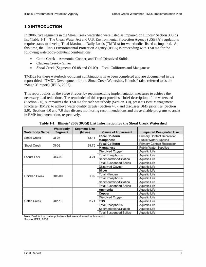
Illinois Environmental Protection Agency Shoal Creek Watershed TMDL Implementation Plan
Final Report 1
1.0 INTRODUCTION
In 2006, five segments in the Shoal Creek watershed were listed as impaired on Illinois’ Section 303(d) list (Table 1-1). The Clean Water Act and U.S. Environmental Protection Agency (USEPA) regulations require states to develop Total Maximum Daily Loads (TMDLs) for waterbodies listed as impaired. At this time, the Illinois Environmental Protection Agency (IEPA) is proceeding with TMDLs for the following waterbody-pollutant combinations:
• Cattle Creek – Ammonia, Copper, and Total Dissolved Solids • Chicken Creek – Silver • Shoal Creek (Segments Ol-08 and Ol-09) – Fecal Coliforms and Manganese
TMDLs for these waterbody-pollutant combinations have been completed and are documented in the report titled, “TMDL Development for the Shoal Creek Watershed, Illinois,” (also referred to as the “Stage 3” report) (IEPA, 2007). This report builds on the Stage 3 report by recommending implementation measures to achieve the necessary load reductions. The remainder of this report provides a brief description of the watershed (Section 2.0), summarizes the TMDLs for each waterbody (Section 3.0), presents Best Management Practices (BMPs) to achieve water quality targets (Section 4.0), and discusses BMP priorities (Section 5.0). Sections 6.0 and 7.0 then discuss monitoring recommendations and the available programs to assist in BMP implementation, respectively.
Table 1-1. Illinois’ 2006 303(d) List Information for the Shoal Creek Watershed
Waterbody Name Waterbody Segment
Segment Size (Miles) Cause of Impairment Impaired Designated Use
Fecal Coliform Primary Contact Recreation Shoal Creek OI-08 13.11 Manganese Public Water Supplies Fecal Coliform Primary Contact Recreation Shoal Creek OI-09 29.75 Manganese Public Water Supplies Dissolved Oxygen Aquatic Life Total Phosphorus Aquatic Life Sedimentation/Siltation Aquatic Life
Locust Fork OlC-02 4.24
Total Suspended Solids Aquatic Life Dissolved Oxygen Aquatic Life Silver Aquatic Life Total Nitrogen Aquatic Life Total Phosphorus Aquatic Life Sedimentation/Siltation Aquatic Life
Chicken Creek OIO-09 1.92
Total Suspended Solids Aquatic Life Ammonia Aquatic Life Copper Aquatic Life Dissolved Oxygen Aquatic Life TDS Aquatic Life Total Phosphorus Aquatic Life Sedimentation/Siltation Aquatic Life
Cattle Creek OIP-10 2.71
Total Suspended Solids Aquatic Life Note: Bold font indicates pollutants that are addressed in this report. Source: IEPA, 2006

Shoal Creek Watershed TMDL Implementation Plan Illinois Environmental Protection Agency
2 Final Report
2.0 DESCRIPTION OF WATERBODY AND WATERSHED CHARACTERISTICS
The purpose of this section of the report is to provide a basic understanding of the Shoal Creek watershed. More detailed information on the soils, topography, land use/land cover, climate and population of the watershed are available in the Stage One Watershed Characterization Report (IEPA, 2007b).
The Shoal Creek watershed is located in south-central Illinois and has a watershed area of approximately 917 square miles. This report addresses the lower portion of the Shoal Creek watershed encompassing 311 square miles (198,859 acres) in Bond, Clinton, and Montgomery Counties. Figure 2-1 shows the portion of the Shoal Creek watershed addressed in this report.
The Illinois Gap Analysis Project Land Cover Data indicate that approximately 130,122 acres, representing 65 percent of the total watershed area, are devoted to agricultural activities (Table 2-1). The majority of the watershed consists of corn and soybean farming (25 percent and 27 percent, respectively). Upland forests occupy 14 percent of the watershed and wetlands occupy approximately 9 percent. Other land cover categories represent 24 percent of the watershed area.
Hydrologic soil groups B, C and D are found within the watershed. Soil erodibility factors reported for these soils in the STATSGO database range from 0.17 to 0.55, indicating moderate soil erodibility. Soils identified by STATSGO as highly erodible generally have slopes greater than 5 percent and represent only 9 percent of the total watershed area.
Table 2-1. Land Use and Land Cover in the Shoal Creek Watershed. Land Cover Category Area (Acres) Percentage
Soybeans 54,177 27.20% Corn 50,174 25.20% Upland 28,618 14.40% Wetlands1 18,320 9.20% Winter Wheat/Soybeans 14,503 7.30% Rural Grassland 13,700 6.90% Winter Wheat 4,757 2.40% Other Small Grains and Hay 4,630 2.30% Forested Areas2 2,941 1.50% Low/Medium Density 2,438 1.20% Other Agriculture 1,881 0.90% High Density 1,278 0.70% Urban Open Space 869 0.50% Surface Water 356 0.20% Barren and Exposed Land 217 0.10% Total 198,859 100% 1. Wetlands includes shallow marsh/wet meadow, deep marsh, floodplain forest, swamp, and shallow water. 2. Forested areas include partial canopy/savannah upland and coniferous.

Illinois Environmental Protection Agency Shoal Creek Watershed TMDL Implementation Plan
Final Report 3
Figure 2-1. Location of the Shoal Creek Watershed

Shoal Creek Watershed TMDL Implementation Plan Illinois Environmental Protection Agency
4 Final Report
3.0 TMDLS AND SOURCES
TMDLs were completed for three waterbodies (four segments) in the Shoal Creek watershed:
• Cattle Creek – Ammonia, Copper, and Total Dissolved Solids • Chicken Creek – Silver • Shoal Creek (Segments Ol-08 and Ol-09) – Fecal Coliforms and Manganese
The following sections summarize the TMDLs and the relevant sources for each waterbody. Source loads and BMP recommendations for each waterbody are presented in Section 5.0. Additional details regarding the TMDLs and sources for each waterbody can be found in the Stage 3 Report (IEPA, 2007).
3.1 Shoal Creek Fecal coliform concentrations in Shoal Creek (Segments OL-08 and OL-09) exceed Illinois’ water quality standard. The TMDL analysis indicates that load reductions are needed during all flow events, ranging from 10 to 94 percent depending on the flow condition. The eight wastewater treatment plants in the watershed are likely the largest sources of fecal coliforms. However, at the time of this report, there were no data from the treatment plants to quantify loads. All eight of the plants have disinfection exemptions. Additional sources of fecal coliforms include animal operations and septic systems.
Manganese concentrations in Shoal Creek also exceed Illinois’ water quality standard. The TMDL analysis indicates that load reductions are needed during most flow events, and range from 0 to 69 percent depending on the flow condition. Streambank erosion and crop production (and associated sediment loads) are likely the largest source of anthropogenic manganese loads.
3.2 Cattle Creek Copper concentrations in Cattle Creek (Segment OLP-10) exceed Illinois’ water quality standard. The TMDL analysis indicates that load reductions are needed during low to mid range flow events. Load reductions range from 0 to 99 percent depending on the flow condition. There are no point sources of copper in the watershed, and the potential nonpoint sources are poorly defined. It is suspected that copper containing fertilizers and/or sediment-bound copper are the anthropogenic sources in Cattle Creek.
Ammonia concentrations in Cattle Creek exceed Illinois’ water quality standard. The TMDL analysis indicates that load reductions are needed during low flow to dry flow events. Load reductions range from 0 to 66 percent, depending on the flow condition. There are no point sources of ammonia in the watershed. Nonpoint sources of ammonia include feed lots, cattle, fertilizers, and septic systems.
Total dissolved solid (TDS) concentrations in Cattle Creek exceed Illinois’ water quality standard. The TMDL analysis indicates that load reductions are needed during low flow to dry flow events. Load reductions range from 0 to 39 percent, depending on the flow condition. There are no point sources of TDS in the watershed. Nonpoint sources of TDS include feed lots, fertilizers, and crop production.
3.3 Chicken Creek Silver concentrations in Chicken Creek (Segment OLO-09) exceed Illinois’ water quality standard. The TMDL analysis indicates that load reductions are needed during mid range flow events (although it should be noted that limited data were available for other flow regimes, and no recent data were available). Load reductions range from 0 to 49 percent depending on the flow condition. There are no point sources of silver in the watershed, and the potential nonpoint sources are poorly defined. It is suspected that sediment-bound silver or other un-identified sources are responsible for the impairment in Chicken Creek.

Illinois Environmental Protection Agency Shoal Creek Watershed TMDL Implementation Plan
Final Report 5
4.0 BEST MANAGEMENT PRACTICES
Controlling pollutant loading to the impaired reaches of the Shoal Creek watershed will require implementation of various BMPs depending on the pollutant(s) of concern and major sources of loading. This section describes the BMPs that may be used to reduce pollutant loading in the Shoal Creek watershed.
4.1 Disinfection of Primary Effluent from Sewage Treatment Plants The majority of the sewage treatment plants in the Shoal Creek watershed operate under a disinfection exemption. Reducing the fecal coliform concentrations from a primary outfall of an exempt facility to 200 cfu/100 mL will require a permit change and disinfection of the effluent prior to discharge. Common disinfection techniques include chlorination, ozonation, and ultraviolet (UV) disinfection. In most cases, chlorination is the most cost-effective alternative, although residuals and oxidized compounds are toxic to aquatic life; subsequent dechlorination may be necessary prior to discharge which will increase costs similar to the other two options (USEPA, 1999b). The options most frequently employed are discussed below.
Illinois EPA is reevaluating disinfection exemption status for NPDES facilities. All facilities that are within three miles of a bacteria impaired segment will be reexamined. The facilities in Table 4-1 will have to reapply for the exemption status at the time of their next permit renewal. This will include submission of new discharge data.
Table 4-1. Facilities that need to reapply for exemption status. Facility Permit Expiration
Germantown STP 12/31/07*
Breese STP 8/31/2009
Pocahantas STP 12/31/07*
Panama STP 12/31/2012
Sorento STP 12/31/07**These permits are going through the renewal process. At the next renewal date they will be required to reapply for exemption status.
4.1.1 Chlorination Chlorine compounds used for disinfection are usually either chlorine gas or hypochlorite solutions though other liquid and solid forms are available. Oxidation of cellular material destroys pathogenic organisms. The remaining chlorine residuals provide additional disinfection, but may also react with organic material to form harmful byproducts. To reduce the impacts on aquatic life from chlorine residuals and byproducts, a dechlorination step is often included in the treatment process (USEPA, 1999b).
The advantages of chlorine disinfection are
• Generally more cost-effective relative to UV disinfection or ozonation • Residuals continue to provide disinfection after discharge • Effective against a wide array of pathogens • Capable of oxidizing some organic and inorganic compounds • Provides some odor control • Allows for flexible dosing

Shoal Creek Watershed TMDL Implementation Plan Illinois Environmental Protection Agency
6 Final Report
There are several disadvantages as well:
• Chlorine residuals are toxic to aquatic life and may require dechlorination, which may increase costs by 30 to 50 percent
• Highly corrosive and toxic with expensive shipping and handling costs • Meeting Uniform Fire Code requirements can increase costs by 25 percent • Oxidation of some organic compounds can produce toxic byproducts • Effluent has increased concentrations of dissolved solids and chloride
More information about disinfection with chlorine is available online at http://www.consolidatedtreatment.com/manuals/Fact_sheet_chlorine_disinfection.pdf
4.1.2 Ozonation Ozone is generated onsite by passing a high voltage current through air or pure oxygen (USEPA, 1999c). The resulting gas (O3) provides disinfection by destroying the cell wall, damaging DNA, and breaking carbon bonds. The advantages of ozonation include
• Ozone is more effective than chlorine and has no harmful residuals. • Ozone is generated onsite so there are no hazardous transport issues. • Short contact time of 10 to 30 minutes. • Elevates the DO of the effluent.
Disadvantages are
• More complex technology than UV light or chlorine disinfection. • Highly reactive and corrosive. • Not economical for wastewater with high concentrations of BOD, TSS, COD, or TOC. • Initial capital, maintenance, and operating costs are typically higher than for UV light or chlorine
disinfection.
More information about ozonation is available online at http://www.epa.gov/owmitnet/mtb/ozon.pdf
4.1.3 Ultraviolet Disinfection UV radiation is generated by passing an electrical current through a lamp containing mercury vapor. The radiation attacks the genetic material of the organisms, destroying reproductive capabilities (NSFC, 1998).
The advantages of UV disinfection are
• Highly effective. • Destruction of pathogens occurs by physical process, so no chemicals must be transported or
stored. • No harmful residuals. • Easy to operate. • Short contact time (20 to 30 min). • Requires less space than chlorination or ozonation.
Disadvantages of UV disinfection are
• Organisms can sometimes regenerate • Turbidity and TSS can interfere with disinfection at high concentrations

Illinois Environmental Protection Agency Shoal Creek Watershed TMDL Implementation Plan
Final Report 7
• Not as cost effective compared to chlorination alone, but when fire code regulations and dechlorination are considered, costs are comparable.
More information about disinfection with UV radiation is available online at http://www.nsfc.wvu.edu/nsfc/pdf/eti/UV_Dis_tech.pdf

Shoal Creek Watershed TMDL Implementation Plan Illinois Environmental Protection Agency
8 Final Report
4.1.4 Effectiveness The use of disinfection techniques in the sewage treatment plants that operate under a disinfection exemption will help in reducing in-stream fecal coliform concentrations to 200 cfu/100 mL.
4.1.5 Costs Upgrading the existing wastewater treatment plants to include disinfection prior to discharge can be achieved with chlorination, ozonation, or UV radiation processes. The costs associated with these three techniques include upfront capital costs to construct additional process units, operating and maintenance costs for chemicals, electricity, labor, etc., as well as chemical storage and fire code requirements associated with the chlorination option. USEPA compares the costs of chlorination, ozonation, and UV disinfection in a series of fact sheets available online. This information is summarized below as well as in Table 4-2. Prices in the fact sheets were listed in either 1995 or 1998 dollars. Prices have been converted to year 2004 dollars, assuming a 3 percent per year inflation rate, for comparison with the other BMPs discussed in this plan that must be described in year 2004 dollars.
Chlorine dosage usually ranges from 5 mg/L to 20 mg/L depending on the wastewater characteristics and desired level of disinfection. The cost of adding a chlorination/dechlorination system that meets fire code requirements and treats one million gallons per day (MGD) of wastewater with a chlorine dosage of 10 mg/L costs approximately $1,260,000 in 1995 with annual operation and maintenance costs of $59,200 (USEPA, 1999b). If a 3 percent per year inflation rate is assumed, these costs in 2004 dollars are $1,640,000 and $77,200, respectively.
Costs for ozonation were given by USEPA (1999c) in 1998 dollars. The capital costs in 1998 for treating one MGD of secondary wastewater with BOD and TSS concentrations each less than 30 mg/L was $300,000. The operating and maintenance costs were listed at $18,500 plus the costs of electricity. In 2004 dollars, these costs are $358,200 and $22,000, respectively.
Ultraviolet radiation costs were listed in 1995 dollars by USEPA (1995) relative to the cost per bulb. Based on vendor information available online, approximately 40 bulbs would be required to treat 1 MGD of secondary wastewater. Based on the information presented, the capital costs in 2004 for a 1 MGD facility would be approximately $750,000 and the annual operating and maintenance costs would range from $4,500 to $5,100.
Table 4-2 compares the costs for these three disinfection technologies. Annualized costs are calculated assuming a 20-year system life for each technology before major repairs or replacement would be required.
Table 4-2. Comparison of Disinfection Costs (2004) per 1 MGD of Sewage Treatment Plant Effluent.
Technology Capital Cost Annual Operating and
Maintenance Cost Annualized Cost
Chlorination (10 mg/L dosage), dechlorination, fire code regulations
$1,640,000 $77,200 $159,200
Ozonation $358,200 $22,000 $39,900, plus cost of electricity
UV Disinfection $750,000 $4,500 to $5,100 $42,000 to $42,600

Illinois Environmental Protection Agency Shoal Creek Watershed TMDL Implementation Plan
Final Report 9
4.2 Proper Maintenance of Onsite Systems The most effective BMP for managing loads from septic systems is regular maintenance. Unfortunately, most people do not think about their wastewater systems until a major malfunction occurs (i.e., sewage backs up into the house or onto the lawn). When not maintained properly, septic systems can cause the release of pathogens and excess nutrients into surface water. Good housekeeping measures relating to septic systems are listed below (Goo, 2004):
• Inspect system annually and pump system every 3 to 5 years, depending on the tank size and number of residents per household.
• Refrain from trampling the ground or using heavy equipment above a septic system (to prevent collapse of pipes).
• Prevent septic system overflow by conserving water, not diverting storm drains or basement pumps into septic systems, and not disposing of trash through drains or toilets.
Education is a crucial component of reducing pollution from septic systems. Many owners are not familiar with USEPA recommendations concerning maintenance schedules. Education can occur through public meetings, mass mailings, and radio and television advertisements. The USEPA recommends that septic tanks be pumped every 3 to 5 years depending on the tank size and number of residents in the household (USEPA, 2002b). Annual inspections, in addition to regular maintenance, ensure that systems are functioning properly. An inspection program would help identify those systems that are currently connected to tile drain systems. All tanks discharging to tile drainage systems should be disconnected immediately.
Some communities choose to formally regulate septic systems by creating a database of all the systems in the area. This database usually contains information on the size, age, and type of system. All inspections and maintenance records are maintained in the database through cooperation with licensed maintenance and repair companies. These databases allow the communities to detect problem areas and ensure proper maintenance.
At this time, there is not a formal inspection and maintenance program in Jackson County. The County Health Department does issue permits for new onsite systems and major repairs
4.2.1 Effectiveness The reductions in pollutant loading resulting from improved operation and maintenance of all systems in the watershed depends on the wastewater characteristics and the level of failure present in the watershed.
4.2.2 Costs Septic tanks are designed to accumulate sludge in the bottom portion of the tank while allowing water to pass into the drain field. If the tank is not pumped out regularly, the sludge can accumulate and eventually become deep enough to enter the drain field. Pumping the tank every three to five years prolongs the life of the system by protecting the drain field from solid material that may cause clogs and system backups.
The cost to pump a septic tank ranges from $250 to $350 depending on how many gallons are pumped out and the disposal fee for the area. If a system is pumped once every three to five years, this expense averages out to less than $100 per year. Septic systems that are not maintained will likely require replacement which may cost between $2,000 and $10,000.
The cost of developing and maintaining a watershed-wide database of the onsite wastewater treatment systems in the Shoal Creek watershed depends on the number of systems that need to be inspected. After the initial inspection of each system and creation of the database, only systems with no subsequent

Shoal Creek Watershed TMDL Implementation Plan Illinois Environmental Protection Agency
10 Final Report
maintenance records would need to be inspected. A recent inspection program in South Carolina found that inspections cost approximately $160 per system (Hajjar, 2000).
Education of home and business owners that use onsite wastewater treatment systems should occur periodically. Public meetings, mass mailings, and radio, newspaper, and TV announcements can all be used to remind and inform owners of their responsibility to maintain their systems. The costs associated with education and inspection programs will vary depending on the level of effort required to communicate the importance of proper maintenance and the number of systems in the area.
The costs associated with inspecting and maintaining onsite wastewater treatment systems and educating owners of their responsibilities is summarized in Table 4-3.
Table 4-3. Costs Associated with Maintaining and Replacing an Onsite Wastewater Treatment System
Action Cost per System Frequency Annual Cost per System
Pumping $250 to $350 Once every 3 to 5 years $70 to $85
Inspection $160 Initially all systems should be inspected, followed by 5 year inspections for systems not on record as being maintained
Up to $32, assuming all systems have to be inspected once every five years, which is not likely
Replacement $2,000 to $10,000 With proper maintenance, system life should be 30 years
$67 to $333
Education $1 Public reminders should occur once per year $1
4.3 Tillage Practices Conservation tillage practices and residue management are commonly used to control erosion and surface transport of pollutants from fields used for crop production. The residuals not only provide erosion control, but also provide a nutrient source to growing plants, and continued use of conservation tillage results in a more productive soil with higher organic and nutrient content. Increasing the organic content of soil has the added benefit of reducing the amount of carbon in the atmosphere by storing it in the soil. Researchers estimate that croplands and pasturelands could be managed to trap 5 to 17 percent of the greenhouse gases produced in the United States (Lewandrowski et al., 2004).
Several practices are commonly used to maintain surface residues:
• No-till systems disturb only a small row of soil during planting, and typically use a drill or knife to plant seeds below the soil surface.
• Strip till operations leave the areas between rows undisturbed, but remove residual cover above the seed to allow for proper moisture and temperature conditions for seed germination.
• Ridge till systems leave the soil undisturbed between harvest and planting: cultivation during the growing season is used to form ridges around growing plants. During or prior to the next planting, the top half to two inches of soil, residuals, and weed seeds are removed, leaving a relatively moist seed bed.
• Mulch till systems are any practice that results in at least 30 percent residual surface cover, excluding no-till and ridge till systems.

Illinois Environmental Protection Agency Shoal Creek Watershed TMDL Implementation Plan
Final Report 11
The NRCS provides additional information on these conservation tillage practices: no-till and strip till: http://efotg.nrcs.usda.gov/references/public/IL/329a.pdf
ridge till: http://efotg.nrcs.usda.gov/references/public/IL/329b.pdf mulch till: http://efotg.nrcs.usda.gov/references/public/IL/329c.pdf
Corn residues are more durable and capable of sustaining the required 30 percent cover required for conservation tillage. Soybeans generate less residue, the residue degrades more quickly, and supplemental measures or special care may be necessary to meet the 30 percent cover requirement (UME, 1996). Figure 4-1 shows a comparison of ground cover under conventional and conservation tillage practices.
Figure 4-1. Comparison of conventional (left) and conservation (right) tillage practices.
4.3.1 Effectiveness Czapar et al. (2006) summarize past and present tillage practices and their impacts on erosion control and nutrient delivery. Historically, the mold board plow was used to prepare the field for planting. This practice disturbed 100 percent of the soil surface and resulted in basically no residual material. Today, conventional tillage typically employs the chisel plow, which is not as disruptive to the soil surface and tends to leave a small amount of residue on the field (0 to 15 percent). Mulch till systems were classified as leaving 30 percent residue; percent cover was not quantified for the no-till systems in this study. The researchers used WEPP modeling to simulate changes in sediment and nutrient loading for these tillage practices. Relative to mold board plowing, chisel plowing reduced phosphorus loads leaving the field by 38 percent, strip tilling reduced loads by 80 percent, and no-till reduced loads by 85 percent. If chisel plowing is now considered conventional, then the strip till and no-till practices are capable of reducing phosphorus loads by 68 percent and 76 percent, respectively (Czapar et al., 2006).
USEPA (2003) reports the findings of several studies regarding the impacts of tillage practices on nutrient, sediment, and manganese loading. The reductions achieved by conservation tillage reported in these studies are summarized below:
• 50 percent reduction in sediment, and likely manganese, silver, copper and TDS, for practices leaving 20 to 30 percent residual cover.
• 90 percent reduction in sediment, and likely manganese, silver, copper and TDS for practices leaving 70 percent residual cover.
• 69 percent reduction in runoff losses for no-till practices.
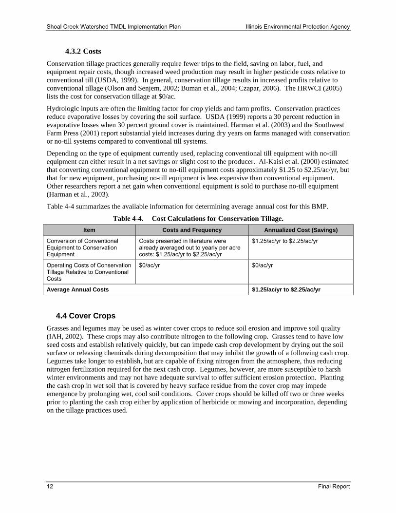
Shoal Creek Watershed TMDL Implementation Plan Illinois Environmental Protection Agency
12 Final Report
4.3.2 Costs Conservation tillage practices generally require fewer trips to the field, saving on labor, fuel, and equipment repair costs, though increased weed production may result in higher pesticide costs relative to conventional till (USDA, 1999). In general, conservation tillage results in increased profits relative to conventional tillage (Olson and Senjem, 2002; Buman et al., 2004; Czapar, 2006). The HRWCI (2005) lists the cost for conservation tillage at $0/ac.
Hydrologic inputs are often the limiting factor for crop yields and farm profits. Conservation practices reduce evaporative losses by covering the soil surface. USDA (1999) reports a 30 percent reduction in evaporative losses when 30 percent ground cover is maintained. Harman et al. (2003) and the Southwest Farm Press (2001) report substantial yield increases during dry years on farms managed with conservation or no-till systems compared to conventional till systems.
Depending on the type of equipment currently used, replacing conventional till equipment with no-till equipment can either result in a net savings or slight cost to the producer. Al-Kaisi et al. (2000) estimated that converting conventional equipment to no-till equipment costs approximately $1.25 to $2.25/ac/yr, but that for new equipment, purchasing no-till equipment is less expensive than conventional equipment. Other researchers report a net gain when conventional equipment is sold to purchase no-till equipment (Harman et al., 2003).
Table 4-4 summarizes the available information for determining average annual cost for this BMP.
Table 4-4. Cost Calculations for Conservation Tillage. Item Costs and Frequency Annualized Cost (Savings)
Conversion of Conventional Equipment to Conservation Equipment
Costs presented in literature were already averaged out to yearly per acre costs: $1.25/ac/yr to $2.25/ac/yr
$1.25/ac/yr to $2.25/ac/yr
Operating Costs of Conservation Tillage Relative to Conventional Costs
$0/ac/yr $0/ac/yr
Average Annual Costs $1.25/ac/yr to $2.25/ac/yr
4.4 Cover Crops Grasses and legumes may be used as winter cover crops to reduce soil erosion and improve soil quality (IAH, 2002). These crops may also contribute nitrogen to the following crop. Grasses tend to have low seed costs and establish relatively quickly, but can impede cash crop development by drying out the soil surface or releasing chemicals during decomposition that may inhibit the growth of a following cash crop. Legumes take longer to establish, but are capable of fixing nitrogen from the atmosphere, thus reducing nitrogen fertilization required for the next cash crop. Legumes, however, are more susceptible to harsh winter environments and may not have adequate survival to offer sufficient erosion protection. Planting the cash crop in wet soil that is covered by heavy surface residue from the cover crop may impede emergence by prolonging wet, cool soil conditions. Cover crops should be killed off two or three weeks prior to planting the cash crop either by application of herbicide or mowing and incorporation, depending on the tillage practices used.

Illinois Environmental Protection Agency Shoal Creek Watershed TMDL Implementation Plan
Final Report 13
(Photo Courtesy of CCSWCD)
Figure 4-2. Use of Cover Crops
The NRCS provides additional information on cover crops at:
http://efotg.nrcs.usda.gov/references/public/IL/340.pdf
4.4.1 Effectiveness The effectiveness of cover crops in reducing pollutant loading has been reported by several agencies. In addition to these benefits, the reduction in runoff losses will reduce erosion from streambanks, further reducing manganese loads and allowing for the establishment of vegetation and canopy cover. The reported reductions are listed below:
• 50 percent reduction in soil and runoff losses with cover crops alone. When combined with no-till systems, may reduce soil loss by more than 90 percent (IAH, 2002). Manganese, silver, copper, and TDS reductions will likely be similar.
• Useful in conservation tillage systems following low-residue crops such as soybeans (USDA, 1999).
4.4.2 Costs The National Sustainable Agriculture Information Service recommends planting ryegrass after corn harvest and hairy vetch after soybeans (Sullivan, 2003). Both seeds can be planted at a depth of ¼ to ½ inch at a rate of 20 lb/ac or broadcast at a rate of 25 to 30 lb/ac (Ebelhar and Plumer, 2007; OSUE, 1990).
Researchers at Purdue University estimate the seed cost of ryegrass and hairy vetch at $12 and $30/ac, respectively. Savings in nitrogen fertilizer (assuming nitrogen fertilizer cost of $0.30/lb (Sample, 2007))

Shoal Creek Watershed TMDL Implementation Plan Illinois Environmental Protection Agency
14 Final Report
are $3.75/ac for ryegrass and $28.50/ac for hairy vetch. Yield increases in the following crop, particularly during droughts, are reported at 10 percent and are expected to offset the cost of this practice (Mannering et al., 1998). Herbicide application is estimated to cost $14.25/ac.
Accounting for the seed cost, herbicide cost, and fertilizer offset results in an average net cost of approximately $19.25/ac assuming that cover crop planting recommendations for a typical 2 year corn/soybean rotation are followed (Mannering et al., 1998). These costs do not account for yield increases which may offset the costs completely. Table 4-5 summarizes the costs and savings associated with ryegrass and hairy vetch.
Table 4-5. Cost Calculations for Cover Crops. Item Ryegrass Hairy Vetch
Seed Costs $12/ac $30/ac
Nitrogen Fertilizer Savings ($3.75/ac) ($28.50/ac)
Herbicide Costs $14.25/ac $14.25/ac
Annual Costs $22.50/ac $15.75/ac
Average Annual Cost Assuming Ryegrass Follows Corn and Hairy Vetch Follows Soybeans: $19.25/ac
4.5 Filter Strips Filter strips are used in agricultural and urban areas to intercept and treat runoff before it leaves the site. If topography allows, filter strips may also be used to treat effluent from tile drain outlets. For small dairy operations, filter strips may also be used to treat milk house washings and runoff from the open lot (NRCS, 2003).
Filter strips will require maintenance, including grading and seeding, to ensure distributed flow across the filter and protection from erosion. Periodic removal of vegetation will encourage plant growth and uptake and remove nutrients stored in the plant material. Filter strips are most effective on sites with mild slopes of generally less than 5 percent, and to prevent concentrated flow, the upstream edge of a filter strip should follow one elevation contour (NCDENR, 2005). A grass filter strip is shown in Figure 4-3. Filter strips also serve to reduce the quantity and velocity of runoff. Filter strip sizing is dependent on site specific features such as climate and topography, but at a minimum, the area of a filter strip should be no less than 2 percent of the drainage area for agricultural land (OSUE, 1994). The minimum filter strip width suggested by NRCS (2002a) is 30 ft. The strips are assumed to function properly with annual maintenance for 30 years before requiring replacement of soil and vegetation.

Illinois Environmental Protection Agency Shoal Creek Watershed TMDL Implementation Plan
Final Report 15
(Photo Courtesy of NRCS)
Figure 4-3. Grass Filter Strip Protecting Stream from Adjacent Agriculture.
4.5.1 Effectiveness Filter strips have been found to effectively remove pollutants from agricultural runoff. The following reductions are reported in the literature (USEPA, 2003; Kalita, 2000; Woerner et al., 2006):
• 55 to 87 percent reduction in fecal coliform
• 65 percent reductions for sediment (and likely manganese, silver, copper and TDS)
• Slows runoff velocities and may reduce runoff volumes via infiltration
• 70 percent reduction in total nitrogen (practices that control nitrogen loading are also expected to control total ammonia concentrations, mainly ammonium).
4.5.2 Costs Filter strips cost approximately $0.30 per sq ft to construct, and the system life is typically assumed to be 20 years (Weiss et al., 2007). Assuming that the required filter strip area is 2 percent of the area drained (OSUE, 1994), 870 square feet of filter strip are required for each acre of agricultural land treated. The construction cost to treat one acre of land is therefore $261/ac. The annualized construction costs are $13/ac/yr. Annual maintenance of filter strips is estimated at $0.01 per sq ft (USEPA, 2002c), for an additional cost of $8.70/ac/yr of agricultural land treated. In addition, the area converted from agricultural production to filter strip will result in a net annual income loss of $3.50. Table 4-6 summarizes the costs assumptions used to estimate the annualized cost to treat one acre of agricultural drainage with a filter strip.

Shoal Creek Watershed TMDL Implementation Plan Illinois Environmental Protection Agency
16 Final Report
Table 4-6. Cost Calculations for Filter Strips Used in Crop Production.
Item Costs Required to Treat One Acre of
Agricultural Land with Filter Strip
Construction Costs $0.30
Annual Maintenance Costs $0.01
Construction Costs $261
System Life (years) 20
Annualized Construction Costs $13
Annual Maintenance Costs $8.70
Annual Income Loss $3.50
Average Annual Costs $25/ac treated
Filter strips used in animal operations typically treat contaminated runoff from pastures or feedlot areas or washings from the milk houses of small dairy operations (NRCS, 2003). The NRCS (2003) costs for small dairy operations (75 milk cows) assumes that a filter strip area of 12,000 square feet is required. For the pasture operations, it is assumed that a filter strip area of 12,000 square feet (30 ft wide and 400 ft long) would be required to treat runoff from a herd of 50 cattle (NRCS, 2003). The document does not explain why more animals can be treated by the same area of filter strip at the dairy operation compared to the pasture operation.
For animal operations, it is not likely that land used for growing crops would be taken out of production for conversion to a filter strip. Table 4-7 summarizes the capital, maintenance, and annualized costs for filter strips per head of animal.
Table 4-7. Cost Calculations for Filter Strips Used at Animal Operations.
Operation Capital Costs per Head
Annual Operation and Maintenance Costs
per Head Total Annualized Costs per Head
Small dairy (75 milking cows) $48 per head of cattle $1.50 per head of cattle $4 per head of cattle
Beef or other (50 cattle) $72 per head of cattle $2.50 per head of cattle $6 per head of cattle
4.6 Grassed Waterways Grassed waterways are stormwater conveyances lined with grass that prevent erosion of the transport channel. In addition, the grassed channel reduces runoff velocities, allows for some infiltration, and filters out some particulate pollutants. Grassed waterways are used in animal operations to divert clean water away from pastures, feedlots, and manure storage areas. A grassed waterway providing surface drainage for a corn field is shown in Figure 4-4.

Illinois Environmental Protection Agency Shoal Creek Watershed TMDL Implementation Plan
Final Report 17
(Photo Courtesy of CCSWCD)
Figure 4-4. Grassed Waterway.
The NRCS provides additional information on grassed waterways at: http://efotg.nrcs.usda.gov/references/public/IL/412.pdf
4.6.1 Effectiveness The effectiveness of grass swales for treating agricultural runoff has not been quantified. The Center for Watershed Protection reports the following reductions in urban settings (Winer, 2000):
• 5 percent reduction in fecal coliform
• 68 percent reduction of total suspended solids (and likely manganese, silver, copper and TDS)
4.6.2 Cost Grassed waterways cost approximately $0.50 per sq ft to construct (USEPA, 2002c). These stormwater conveyances are best constructed where existing bare ditches transport stormwater, so no income loss from land conversion is expected with this practice. It is assumed that the average area required for a grassed waterway is approximately 0.1 to 0.3 percent of the drainage area, or between 44 and 131 sq ft per acre. The range is based on examples in the Illinois Drainage Guide, information from the NRCS Engineering Field Handbook, and a range of waterway lengths (100 to 300 feet). Waterways are assumed to remove phosphorus effectively for 20 years before soil, vegetation, and drainage material need to be replaced (Weiss et al., 2007). The construction cost spread out over the life of the waterway is thus $2.25/yr for each acre of agriculture draining to a grassed waterway. Annual maintenance of grassed waterways is estimated at $0.02 per sq ft (Rouge River, 2001) for an additional cost of $1.75/ac/yr of agricultural land treated. Table 4-8 summarizes the annual costs assumptions for grassed waterways.

Shoal Creek Watershed TMDL Implementation Plan Illinois Environmental Protection Agency
18 Final Report
Table 4-8. Cost Calculations for Grassed Waterways in Agricultural Land. Item Costs Required to Treat One Acre of Agricultural Land
Cost per Square Foot
Construction Costs $0.50
Annual Maintenance Costs $0.02
Cost to Treat One Acre of Agricultural Land (assuming 44 to 131 sq ft of filter strip)
Construction Costs $22 to $65.50
System Life (years) 20
Annualized Construction Costs $1 to $3.25
Annual Maintenance Costs $1 to $2.75
Annual Income Loss $0
Average Annual Cost $2 to 6/ac treated
Grassed waterways are primarily used in animal operations to divert clean water away from pastures, feedlots, and manure storage areas. Table 4-9 summarizes the capital, maintenance, and annualized costs of this practice per head of cattle as summarized by NRCS (2003).
Table 4-9. Cost Calculations for Grassed Waterways Used in Cattle Operations.
Capital Cost per Head Annual Operation and Maintenance
Cost per Head Total Annualized Cost per Head
$0.50 to $1.50 $0.02 to $0.04 $0.05 to $0.12
4.7 Riparian Buffers Riparian corridors, including both the stream channel and adjacent land areas, are important components of watershed ecology. The streamside forest slowly releases nutrients as twigs and leaves decompose. These nutrients are valuable to the fungi, bacteria, and invertebrates that form the basis of a stream’s food chain. Tree canopies of riparian forests also cool the water in streams which can affect the composition of the fish species in the stream, the rate of biological reactions, and the amount of dissolved oxygen the water can hold. Channelization or widening of streams moves the canopy farther apart, decreasing the amount of shaded water surface, increasing water temperatures, and decreasing dissolved oxygen concentrations.
Preserving the natural vegetation along a stream corridor can mitigate pollutant loading associated with human disturbances. The root structure of the vegetation in a buffer enhances infiltration and subsequent trapping of nonpoint source pollutants. However, the buffers are only effective in this manner when the runoff enters the buffer as a slow moving, shallow “sheet”; concentrated flow in a ditch or gully will quickly pass through the buffer offering minimal opportunity for retention and uptake of pollutants.
Even more important than the filtering capacity of the buffers is the protection they provide to streambanks. The rooting systems of the vegetation serve as reinforcements in streambank soils, which help to hold streambank material in place and minimize erosion. Riparian buffers also prevent cattle access to streams, reducing streambank trampling and defecation in the stream. Due to the increase in stormwater runoff volume and peak rates of runoff associated with agriculture and development, stream channels are subject to greater erosional forces during stormflow events. Thus, preserving natural vegetation along stream channels minimizes the potential for water quality and habitat degradation due to streambank erosion and enhances the pollutant removal of sheet flow runoff from developed areas that

Illinois Environmental Protection Agency Shoal Creek Watershed TMDL Implementation Plan
Final Report 19
pass through the buffer. A riparian buffer protecting the stream corridor from adjacent agricultural areas is shown in Figure 4-5.
Figure 4-5. Riparian Buffer Protecting the Stream from Adjacent Agricultural Fields.
4.7.1 Effectiveness Riparian buffers should consist of native species and may include grasses, forbs, shrubs, and trees. Minimum buffer widths of 25 feet are required for water quality benefits. Higher removal rates are provided with greater buffer widths. Riparian corridors typically treat a maximum of 300 ft of adjacent land before runoff forms small channels that short circuit treatment. Buffer widths based on slope measurements and recommended plant species should conform to NRCS Field Office Technical Guidelines. The following reductions are reported in the literature:
• 34 to 74 percent reduction of fecal coliform for 30 ft wide buffers (Wenger, 1999).
• 87 percent reduction of fecal coliform for 200 ft wide buffers (Wenger, 1999).
• 70 to 90 percent reduction of sediment (and likely manganese, silver, copper and TDS) (NCSU, 2002).
• 74 percent reduction of total nitrogen for 30 ft wide buffer (Dillaha et al, 1989).
• Increased channel stability will reduce streambank erosion and manganese, silver, copper and TDS loads.
4.7.2 Costs Restoration of riparian areas costs approximately $100/ac to construct and $475/ac to maintain over the life of the buffer (Wossink and Osmond, 2001; NCEEP, 2004). Maintenance of a riparian buffer should be minimal, but may include items such as period inspection of the buffer, minor grading to prevent short
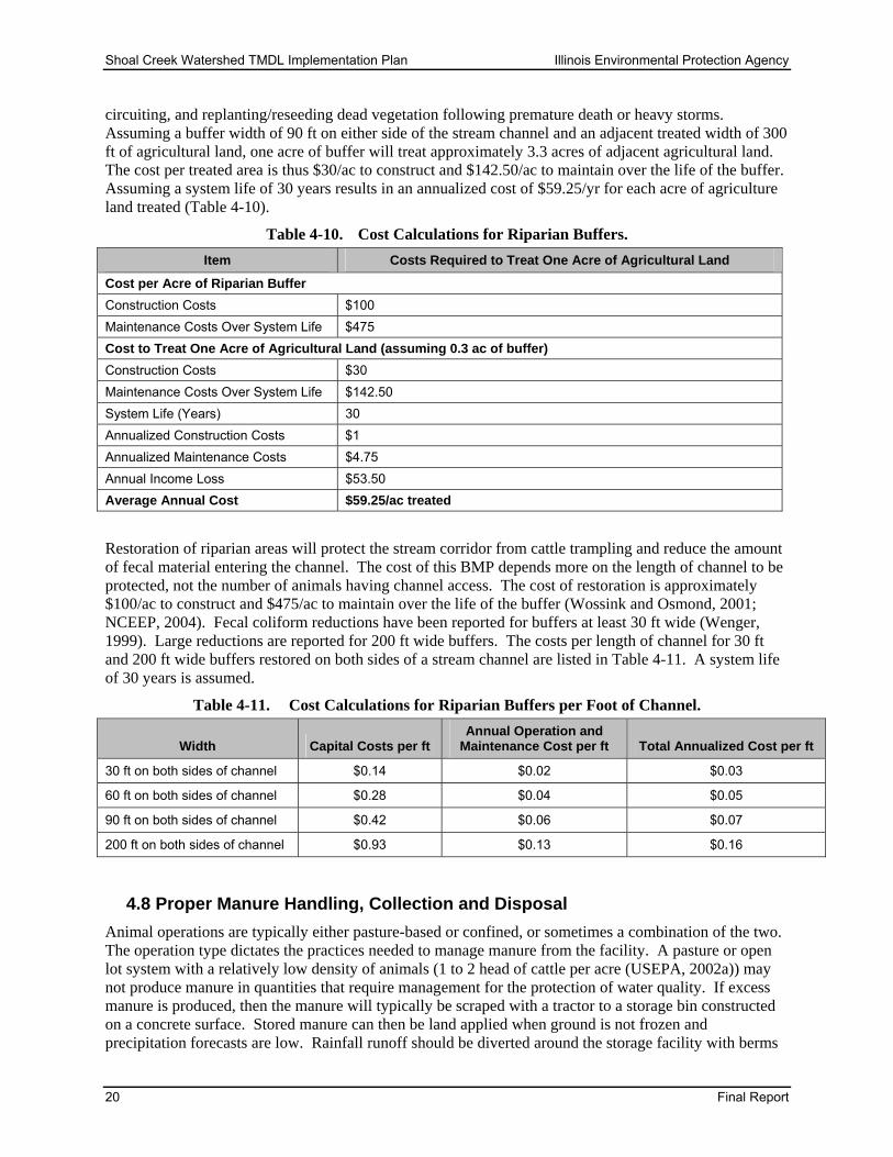
Shoal Creek Watershed TMDL Implementation Plan Illinois Environmental Protection Agency
20 Final Report
circuiting, and replanting/reseeding dead vegetation following premature death or heavy storms. Assuming a buffer width of 90 ft on either side of the stream channel and an adjacent treated width of 300 ft of agricultural land, one acre of buffer will treat approximately 3.3 acres of adjacent agricultural land. The cost per treated area is thus $30/ac to construct and $142.50/ac to maintain over the life of the buffer. Assuming a system life of 30 years results in an annualized cost of $59.25/yr for each acre of agriculture land treated (Table 4-10).
Table 4-10. Cost Calculations for Riparian Buffers. Item Costs Required to Treat One Acre of Agricultural Land
Cost per Acre of Riparian Buffer Construction Costs $100 Maintenance Costs Over System Life $475 Cost to Treat One Acre of Agricultural Land (assuming 0.3 ac of buffer) Construction Costs $30 Maintenance Costs Over System Life $142.50 System Life (Years) 30 Annualized Construction Costs $1 Annualized Maintenance Costs $4.75 Annual Income Loss $53.50 Average Annual Cost $59.25/ac treated
Restoration of riparian areas will protect the stream corridor from cattle trampling and reduce the amount of fecal material entering the channel. The cost of this BMP depends more on the length of channel to be protected, not the number of animals having channel access. The cost of restoration is approximately $100/ac to construct and $475/ac to maintain over the life of the buffer (Wossink and Osmond, 2001; NCEEP, 2004). Fecal coliform reductions have been reported for buffers at least 30 ft wide (Wenger, 1999). Large reductions are reported for 200 ft wide buffers. The costs per length of channel for 30 ft and 200 ft wide buffers restored on both sides of a stream channel are listed in Table 4-11. A system life of 30 years is assumed.
Table 4-11. Cost Calculations for Riparian Buffers per Foot of Channel.
Width Capital Costs per ft Annual Operation and
Maintenance Cost per ft Total Annualized Cost per ft
30 ft on both sides of channel $0.14 $0.02 $0.03
60 ft on both sides of channel $0.28 $0.04 $0.05
90 ft on both sides of channel $0.42 $0.06 $0.07
200 ft on both sides of channel $0.93 $0.13 $0.16
4.8 Proper Manure Handling, Collection and Disposal Animal operations are typically either pasture-based or confined, or sometimes a combination of the two. The operation type dictates the practices needed to manage manure from the facility. A pasture or open lot system with a relatively low density of animals (1 to 2 head of cattle per acre (USEPA, 2002a)) may not produce manure in quantities that require management for the protection of water quality. If excess manure is produced, then the manure will typically be scraped with a tractor to a storage bin constructed on a concrete surface. Stored manure can then be land applied when ground is not frozen and precipitation forecasts are low. Rainfall runoff should be diverted around the storage facility with berms

Illinois Environmental Protection Agency Shoal Creek Watershed TMDL Implementation Plan
Final Report 21
or grassed waterways. Runoff from the feedlot area is considered contaminated and is typically treated in a lagoon.
Confined facilities (typically dairy cattle, swine, and poultry operations) often collect manure in storage pits located under slatted floors. Wash water used to clean the floors and remove manure buildup combines with the solid manure to form a liquid or slurry in the pit. The mixture is usually land applied or transported offsite.
Final disposal of waste usually involves land application on the farm or transportation to another site. Manure is typically applied to the land once or twice per year. To maximize the amount of nutrients and organic material retained in the soil, application should not occur on frozen ground or when precipitation is forecast during the next several days.
An example of a waste storage lagoon is shown in Figure 4-6.
Figure 4-6. Waste Storage Lagoon.
The NRCS provides additional information on waste storage facilities and cover at
http://efotg.nrcs.usda.gov/treemenuFS.aspx in Section IV B. Conservation Practices Number 313 and 367
and on anaerobic lagoons at http://efotg.nrcs.usda.gov/references/public/IL/IL-365_2004_09.pdf http://efotg.nrcs.usda.gov/references/public/IL/IL-366_2004_09.pdf

Shoal Creek Watershed TMDL Implementation Plan Illinois Environmental Protection Agency
22 Final Report
4.8.1 Effectiveness Though little change in total phosphorus or organic content has been reported, reductions in fecal coliform as a result of manure storage have been documented in two studies:
• 97 percent reduction in fecal coliform concentrations in runoff when manure is stored for at least 30 days prior to land application (Meals and Braun, 2006).
• 90 percent reduction in fecal coliform loading with the use of waste storage structures, ponds, and lagoons (USEPA, 2003).
4.8.2 Costs Depending on whether or not the production facility is pasture-based or confined, manure is typically deposited in feedlots, around watering facilities, and within confined spaces such as housing units and milking parlors. Except for feedlots serving a low density of animals, each location will require the collection and transport of manure to a storage structure, holding pond, storage pit, or lagoon prior to final disposal.
Manure collected from open lots and watering areas is typically collected by a tractor equipped with a scraper. This manure is in solid form and is typically stored on a concrete pad surrounded by three walls that allow for stacking of contents. Depending on the climate, a roof may be required to protect the manure from frequent rainfall. Clean water from rooftops or up-grade areas should be diverted around waste stockpiles and heavy use areas with berms, grassed channels, or other means of conveyance (USEPA, 2003). Waste storage lagoons, pits, and above ground tanks are good options for large facilities. Methane gas recovered from anaerobic treatment processes can be used to generate electricity.
The NRCS (2003) has developed cost estimates for the various tasks and facilities typically used to transport, store, and dispose of manure. Table 4-12 summarizes the information contained in the NRCS report and lists the capital and operating/maintenance costs reported per head of animal. Annual maintenance costs were assumed 3 percent of capital costs except for gutter downspouts (assumed 10 percent to account for animals trampling the downspouts) and collection and transfer (assumed 15 percent to account for costs associated with additional fuel and labor). The costs presented as a range were given for various sizes of operations. The lower values reflect the costs per head for the larger operations which are able to spread out costs over more animals.
The full NRCS document can be viewed at http://www.nrcs.usda.gov/Technical/land/pubs/cnmp1.html
The useful life for practices requiring construction is assumed to be 20 years. The total annualized costs were calculated by dividing the capital costs by 20 and adding the annual operation and maintenance costs. Prices are converted to year 2004 dollars.

Illinois Environmental Protection Agency Shoal Creek Watershed TMDL Implementation Plan
Final Report 23
Table 4-12. Costs Calculation for Manure Handling, Storage, and Treatment per Head.
Item Application Capital Cost per
Head
Annual Operation and Maintenance
Cost per Head Total Annualized Cost
per Head
Collection and Transfer of Solid Manure, Liquid/Slurry Manure, and Contaminated Runoff
Collection and transfer of manure solids (assuming a tractor must be purchased)
All operations with outside access and solid collection systems for layer houses
$130.50 - dairy cattle $92.50 - beef cattle $0 - layer1 $37.00 - swine
$19.50 - dairy cattle $13.75 - beef cattle $0.04 - layer $5.50 - swine
$26.00 - dairy cattle $18.25 - beef cattle $0.04 - layer $7.25 - swine
Collection and transfer of liquid/slurry manure
Dairy, swine, and layer operations using a flush system
$160 to $200 - dairy cattle $.50 - layer $5.75 to $4.50 - swine
$12.25 - dairy cattle AAAA $0.03 - layer $0.25 - swine
$20.25 to 22.25 - dairy cattle $0.05 - layer $0.50 - swine
Collection and transfer of contaminated runoff using a berm with pipe outlet
Fattened cattle and confined heifers
$4 to $9 - cattle $0.12 to 0.25 - cattle $0.25 to $0.75 - cattle
Feedlot Upgrades for Cattle Operations Using Concentrated Feeding Areas
Grading and installation of a concrete pad
Cattle on feed (fattened cattle and confined heifers)
$35 - cattle $1 - cattle $2.75 - cattle
Clean Water Diversions
Roof runoff management: gutters and downspouts
Dairy and swine operations that allow outside access
$16 - dairy cattle $2.25 - swine
$1.60 - dairy cattle $0.25 - swine
$2.50 - dairy cattle $0.50 - swine
Earthen berm with underground pipe outlet
Fattened cattle and dairy operations
$25.25 to $34.50 - cattle
$0.75 to $1.00 - cattle $2 to $2.75 - cattle
Earthen berm with surface outlet
Swine operations that allow outside access
$1 - swine $0.03 - swine $0.08 - swine
Grassed waterway Fattened cattle and confined heifer operations: scrape and stack system
$0.50 to $1.50 - cattle
$0.02 to $0.04 - cattle $0.05 to $0.12 - cattle
1 Costs presented by NRCS (2003) as operating and maintenance only.

Shoal Creek Watershed TMDL Implementation Plan Illinois Environmental Protection Agency
24 Final Report
Table 4-12. Cost Calculations for Manure Handling, Storage, and Treatment Per Head (continued).
Item Application Capital Cost per
Head
Annual Operation and Maintenance
Cost per Head Total Annualized Cost
per Head
Storage
Liquid storage (contaminated runoff and wastewater)
Swine, dairy, and layer operations using flush systems (costs assume manure primarily managed as liquid)
$245 to $267 - dairy cattle $2 - layer $78.50 to $80 - swine
$7.25 - dairy cattle AAAA $0.06 - layer $2.50 - swine
$19.50 to $20.50 - dairy cattle $0.16 - layer $6.50 - swine
Slurry storage Swine and dairy operations storing manure in pits beneath slatted floors (costs assume manure primarily managed as slurry)
$104 to $127 - dairy cattle $15.50 to $19.50 - swine
$3.25 to $3.75 - dairy cattle $0.50 - swine
$8.25 to $10.25 - dairy cattle $1.25 to $1.50 - swine
Runoff storage ponds (contaminated runoff)
All operations with outside access
$125.50 - dairy cattle $140 - beef cattle $23 - swine
$3.75 - dairy cattle $4.25 - beef cattle $0.75 - swine
$10 - dairy cattle $11.25 - beef cattle $2 - swine
Solid storage All animal operations managing solid wastes (costs assume 100% of manure handled as solid)
$196 - dairy cattle $129 - beef cattle $1 - layer $14.25 - swine
$5.75 - dairy cattle $3.75 - beef cattle $0.03 - layer $0.50 - swine
$15.50 - dairy cattle $10.25 - beef cattle $0.25 - layer $1.25 - swine

Illinois Environmental Protection Agency Shoal Creek Watershed TMDL Implementation Plan
Final Report 25
Table 4-12. Cost Calculations for Manure Handling, Storage, and Treatment Per Head (continued).
Item Application Capital Cost per
Head
Annual Operation and Maintenance
Cost per Head Total Annualized Cost
per Head
Final Disposal
Pumping and land application of liquid/slurry
Operations handling manure primarily as liquid or slurry.
Land application costs are listed as capital plus operating for final disposal and are listed as dollars per acre for the application system. The required number of acres per head was calculated for each animal type based on the phosphorus content of manure at the time of application. Pumping costs were added to the land application costs as described in the document.
$19.50 - dairy cattle $0.25 - layer $2.75 - swine
Pumping and land application of contaminated runoff
Operations with outside feedlots and manure handled primarily as solid
Pumping costs and land application costs based on information in NRCS, 2003. Assuming a typical phosphorus concentration in contaminated runoff of 80 mg/L to determine acres of land required for agronomic application (Kizil and Lindley, 2000). Costs for beef cattle listed as range representing variations in number of animals and manure handling systems (NRCS, 2003). Only one type and size of dairy and swine operation were included in the NRCS document.
$4 - dairy cattle $3.75 - beef cattle $4.50 - swine
Land application of solid manure
Operations handling manure primarily as solid
Land application costs are listed as capital plus operating for final disposal and are given as dollars per acre for the application system. The required number of acres per head was calculated for each animal type based on the phosphorus content of manure at the time of application. No pumping costs are required for solid manure.
$11 - dairy cattle $0.25 - layer $1.50 - swine $10.25 - fattened cattle
Shoal Creek Watershed TMDL Implementation Plan Illinois Environmental Protection Agency
26 Final Report
4.9 Feeding Strategies Use of dietary supplements, genetically enhanced feed and specialized diets have been found to reduce ammonia emissions from manure. Excess protein that is not utilized by animals is excreted in manure. Since protein contains nitrogen, controlling the amount of protein fed to animals reduces ammonia gas emission. Zeolites and charcoal have been added to swine feeds in an attempt to bind ammonia, and thereby reduce emissions. Studies done on diet manipulation have shown reducing dietary crude protein to be effective in controlling ammonia emission (USEPA, 2001).
4.9.1 Effectiveness Diets that are effective in reducing the protein content in manure are successful in inhibiting ammonia gas emission. Ammonia gas reductions achieved through dietary manipulation are presented below:
• 28 percent reduction in ammonia gas from dairy cows that were fed a die containing 9.5 percent crude protein (Lames et al.; 2000).
• 56 percent reduction in ammonia gas from swine manure by supplementing feed with yucca extract.
4.9.2 Costs Dietary supplements have the potential of reducing feed costs. Reducing intake to dietary requirements established by the USDA may save dairy farmers 25 dollars per year per cow (USEPA, 2002a).
4.10 Composting Composting is the biological decomposition and stabilization of organic material. The process produces heat that, in turn, produces a final product that is stable, free of pathogens and viable plant seeds, and can be beneficially applied to the land. Like manure storage areas, composting facilities should be located on dry, flat, elevated land at least 100 feet from streams. The landowner should coordinate with local NRCS staff to determine the appropriate design for a composting facility based on the amount of manure generated. Extension agents can also help landowners achieve the ideal nutrient ratios, oxygen levels, and moisture conditions for composting on their site.
Composting can be accomplished by simply constructing a heap of the material, forming composting windrows, or by constructing one or more bins to hold the material. Heaps should be 3 feet wide and 5 feet high with the length depending on the amount of manure being composted. Compost does not have to be turned, but turning will facilitate the composting process (University of Missouri, 1993; PSU, 2005). Machinery required for composting includes a tractor, manure spreader, and front-end loader (Davis and Swinker, 2004). Figure 4-7 shows a poultry litter composting facility.

Illinois Environmental Protection Agency Shoal Creek Watershed TMDL Implementation Plan
Final Report 27
(Photo courtesy of USDA NRCS.)
Figure 4-7. Poultry Litter Composting Facility.
The NRCS provides additional information on composting facilities at http://efotg.nrcs.usda.gov/references/public/IL/IL-317rev9-04.pdf
and ftp://ftp.wcc.nrcs.usda.gov/downloads/wastemgmt/neh637c2.pdf
4.10.1 Effectiveness Composting stabilizes the organic content of manure and reduces the volume that needs to be disposed of. In addition, the following reductions in loading are reported:
• 99 percent reduction of fecal coliform concentrations as a result of the heat produced during the composting process (Larney et. al., 2003).
• 56 percent reduction in runoff volumes and 68 percent reduction in sediment (and likely manganese, copper, silver, and TDS) as a result of improved soil infiltration following application of composted manure (HRWCI, 2005).
4.10.2 Costs The costs for developing a composting system include site development costs (storage sheds, concrete pads, runoff diversions, etc.), purchasing windrow turners if that system is chosen, and labor and fuel required to form and turn the piles. Cost estimates for composting systems have not been well documented and show a wide variation even for the same type of system. The NRCS is in the process of developing cost estimates for composting and other alternative manure applications in Part II of the document discussed in Section 4.8.2. Once published, these estimates should provide a good comparison

Shoal Creek Watershed TMDL Implementation Plan Illinois Environmental Protection Agency
28 Final Report
with the costs summarized for the Midwest region in Table 4-12. For now, costs are presented in Table 4-13 based on studies conducted in Wisconsin, Canada, and Indiana.
Researchers in Wisconsin estimated the costs of a windrow composting system using four combinations of machinery and labor (CIAS, 1996). These costs included collection and transfer of excreted material, formation of the windrow pile, turning the pile, and reloading the compost for final disposal. The Wisconsin study was based on a small dairy operation (60 head). Costs for beef cattle, swine, and layer hens were calculated based on animal units and handling weights of solid manure (NRCS, 2003). Equipment life is assumed 20 years. The costs presented in the Wisconsin study are much higher than those presented in Table 4-13 for collection, transfer, and storage of solid manure. However, the Wisconsin study presented a cost comparison of the windrow system to stacking on a remote concrete slab, and these estimates were approximately four and half times higher than the values summarized by NRCS. It is likely that the single data set used for the Wisconsin study is not representative of typical costs.
Two studies have been conducted in Canada regarding the costs of composting. The University of Alberta summarized the per ton costs of windrow composting with a front end load compared to a windrow turner (University of Alberta, 2000). The Alberta Government presented a per ton estimate for a windrow system with turner: this estimate is quite different than the University of Alberta study. These per ton costs were converted to costs per head of dairy cattle, beef cattle, swine, and layer hens based on the manure generation and handling weights presented by NRCS (2003).
In 2001, the USEPA released a draft report titled “Alternative Technologies/Uses for Manure.” This report summarizes results from a Purdue University research farm operating a 400-cow dairy operation. This farm also utilizes a windrow system with turner.
Table 4-13 summarizes the cost estimates presented in each of the studies for the various composting systems. None of these estimates include the final costs of land application, which should be similar to those listed for disposal of solid manure in Table 4-12.
.

Illinois Environmental Protection Agency Shoal Creek Watershed TMDL Implementation Plan
Final Report 29
Table 4-13. Cost Calculations for Manure Composting.
Equipment Used Capital Cost
per Head Annual Operation and
Maintenance Cost per Head Total Annualized Cost
per Head
2004 Cost Estimated from CIAS, 1996 – Wisconsin Study
Windrow composting with front-end loader
$324.25 - dairy cattle $213.50 - beef cattle $1.75 - layer $23.75 - swine
$179.75 - dairy cattle $118.50 - beef cattle $1 - layer $13.25 - swine
$196 - dairy cattle $129.25 - beef cattle $1 - layer $14.25 - swine
Windrow composting with bulldozer
$266 - dairy cattle $175.25 - beef cattle $1.50 - layer $19.50 - swine
$179.75 - dairy cattle $118.50 - beef cattle $1 - layer $13.25 - swine
$193.25 - dairy cattle $127.25 - beef cattle $1 - layer $14.25 - swine
Windrow composting with custom-hire compost turner
$266 - dairy cattle $175.25 - beef cattle $1.50 - layer $19.50 - swine
$215.25 - dairy cattle $141.75 - beef cattle $1.25 - layer $15.75 - swine
$228.75 - dairy cattle $150.50 - beef cattle $1.25 - layer $16.75 - swine
Windrow composting with purchased compost turner
$617 - dairy cattle $406.25 - beef cattle $3.50 - layer $45.25 - swine
$234.25 - dairy cattle $154.25 - beef cattle $1.25 - layer $17.25 - swine
$265.25 - dairy cattle $174.75 - beef cattle $1.50 - layer $19.50 - swine
2004 Costs Estimated from University of Alberta, 2000
Windrow composting with front-end loader
Study presented annualized costs per ton of manure composted.
$23.75 to $47.50 - dairy cattle $15.75 to $31.25 - beef cattle $0.13 to $0.25 - layer $1.75 to $3.50 - swine
Windrow composting with compost turner
Study presented annualized costs per ton of manure composted.
$71.25 to $142.50 - dairy cattle $47.00 to $94.00 - beef cattle $0.50 to $0.75 - layer $5.25 to $10.50 - swine
2004 Costs Estimated from Alberta Government, 2004
Windrow composting with compost turner
Study presented annualized costs per ton of manure composted.
$31.50 - dairy cattle $20.75 - beef cattle $0.25 - layer $2.25 - swine
2004 Costs Estimated from USEPA, 2001 Draft
Windrow composting with compost turner
Study presented annualized costs per dairy cow. $15.50 - dairy cattle $10.25 - beef cattle $0.09 - layer $1.25 - swine

Shoal Creek Watershed TMDL Implementation Plan Illinois Environmental Protection Agency
30 Final Report
4.11 Alternative Watering Systems Landowners often allow animals direct access to streams for their water supply. This can lead to denuded streambanks and riparian vegetation, and may result in manure that is deposited in or near the stream. Alternative watering systems allow animals to access drinking water away from the stream, thereby minimizing the impacts to the stream and riparian corridor.
Landowners should work with an agricultural extension agent to properly design and locate watering facilities. One option is to collect rainwater from building roofs (with gutters feeding into cisterns) and use this water for the animal watering system to reduce runoff and conserve water use (Tetra Tech, 2006). Whether or not animals are allowed access to streams, the landowner should provide an alternative shady location and water source so that animals are encouraged to stay away from riparian areas.
Figure 4-8 shows a centralized watering tank allowing access from rotated grazing plots and a barn area.
(Photo courtesy of USDA NRCS.)
Figure 4-8. Centralized Watering Tank.

Illinois Environmental Protection Agency Shoal Creek Watershed TMDL Implementation Plan
Final Report 31
The NRCS provides additional information on these alternative watering components: Spring development: http://efotg.nrcs.usda.gov/references/public/IL/IL-574.pdf, Well development: http://efotg.nrcs.usda.gov/references/public/IL/IL-642.pdf, Pipeline: http://efotg.nrcs.usda.gov/references/public/IL/516.pdf,
Watering facilities (trough, barrel, etc.): http://efotg.nrcs.usda.gov/treemenuFS.aspx
in Section IV B. Conservation Practices Number 614
4.11.1 Effectiveness The USEPA (2003) reports that the following pollutant load reductions were achieved by supplying cattle with alternative watering locations and excluding cattle from the stream channel by structural or vegetative barrier:
• 29 to 46 percent reductions in fecal coliform loading.
Some researchers have studied the impacts of providing alternative watering sites without structural exclusions and found that cattle spend 90 percent less time in the stream when alternative drinking water is furnished (USEPA, 2003). Prohibiting access to the stream channels will also prevent streambank trampling, decrease bank erosion, protect bank vegetation, and reduce the loading of organic material to the streams. As a result, manganese, copper, silver and TDS loads associated with bank erosion will decrease.
4.11.2 Costs Alternative drinking water can be supplied by installing a well in the pasture area, pumping water from a nearby stream to a storage tank, developing springs away from the stream corridor, or piping water from an existing water supply. For pasture areas without access to an existing water supply, the most reliable alternative is installation of a well, which ensures continuous flow and water quality for the cattle (NRCS, 2003). Assuming a well depth of 250 ft and a cost of installation of $22.50 per ft, the cost to install a well is approximately $5,625 per well. The well pump would be sized to deliver adequate water supply for the existing herd size. For a herd of 150 cattle, the price per head for installation was estimated at $37.50 per head of cattle.
After installation of the well or extension of the existing water supply, a water storage device is required to provide the cattle access to the water. Storage devices include troughs or tanks. NRCS (2003) lists the costs of storage devices at $23 per head.
Annual operating costs to run the well pump range from $9 to $22 per year for electricity (USEPA, 2003; Marsh, 2001), or up to $0.15 per head. Table 4-14 lists the capital, maintenance, and annualized costs for a well, pump, and storage system assuming a system life of 20 years.
Table 4-14. Cost Calculations for Alternative Watering Facilities.
Item Capital Cost per Head
Annual Operation and Maintenance Cost
per Head Total Annualized Cost
per Head
Installation of well $37.50 $0 $2
Storage container $23 $0 $1
Electricity for well pump $0 $0.15 $0.15
Total system costs $60.50 $0.15 $3.15

Shoal Creek Watershed TMDL Implementation Plan Illinois Environmental Protection Agency
32 Final Report
4.12 Cattle Exclusion from Streams Cattle manure can be a substantial source of fecal coliform loading to streams, particularly where direct access is not restricted and/or where cattle feeding structures are located adjacent to riparian areas. Direct deposition of feces into streams may be a primary mechanism of pollutant loading during baseflow periods. During storm events, overbank and overland flow may entrain manure accumulated in riparian areas resulting in pulsed loads of fecal coliform bacteria into streams. In addition, cattle with unrestrained stream access typically cause severe streambank erosion. The impacts of cattle on stream ecosystems are shown in Figure 4-9 and Figure 4-10.
Figure 4-9. Typical Stream Bank Erosion in Pastures with Cattle Access to Stream.
Figure 4-10. Cattle-Induced Streambank Mass Wasting and Deposition of Manure into Stream.

Illinois Environmental Protection Agency Shoal Creek Watershed TMDL Implementation Plan
Final Report 33
An example of proper exclusion and the positive impacts it has on the stream channel are shown in Figure 4-11.
(Photo courtesy of USDA NRCS.)
Figure 4-11. Stream Protected from Sheep by Fencing.
The NRCS provides additional information on fencing at: http://efotg.nrcs.usda.gov/treemenuFS.aspx
in Section IV B. Conservation Practices Number 382
Allowing limited or no animal access to streams will provide the greatest water quality protection. On properties where cattle need to cross streams to have access to pasture, stream crossings should be built so that cattle can travel across streams without degrading streambanks and contaminating streams with manure. Figure 4-12 shows an example of a reinforced cattle access point to minimize time spent in the stream and mass wasting of streambanks.

Shoal Creek Watershed TMDL Implementation Plan Illinois Environmental Protection Agency
34 Final Report
(Photo courtesy of USDA NRCS.)
Figure 4-12. Restricted Cattle Access Point with Reinforced Banks.
The NRCS provides additional information on use exclusion and controlled access at: http://efotg.nrcs.usda.gov/treemenuFS.aspx
in Section IV B. Conservation Practices Number 472
4.12.1 Effectiveness Fencing cattle from streams and riparian areas using vegetative or fencing materials will reduce streambank trampling and direct deposition of fecal material in the streams. As a result, manganese, silver, copper and TDS (associated with eroded sediment) loads will decrease. The USEPA (2003) reports the following reductions in fecal coliform loading as a result of cattle exclusion practices:
• 29 to 46 percent reductions in fecal coliform loading.
4.12.2 Costs The costs of excluding cattle from streams depends more on the length of channel that needs to be protected than the number of animals on site. Fencing may also be used in a grazing land protection operation to control cattle access to individual plots. The system life of wire fences is reported as 20 years; the high tensile fence materials have a reported system life of 25 years (Iowa State University, 2005). NRCS reports that the average operation needs approximately 35 ft of additional fencing per head to protect grazing lands and streams. Table 4-15 presents the capital, maintenance, and annualized costs for four fencing materials based on the NRCS assumptions.

Illinois Environmental Protection Agency Shoal Creek Watershed TMDL Implementation Plan
Final Report 35
Table 4-15. Installation and Maintenance Costs of Fencing Material.
Material Capital Cost
per Head
Annual Operation and Maintenance Cost
per Head Total Annualized
Cost per Head
Woven Wire $43.50 $3.50 $5.75
Barbed Wire $33.50 $2.75 $4.50
High Tensile (non-electric) 8-strand $30.75 $1.75 $3.00
High Tensile (electric) 5-strand $23.00 $1.50 $2.50
4.13 Grazing Land Management While erosion rates from pasture areas are generally lower than those from row-crop areas, a poorly managed pasture can approach or exceed a well-managed row-crop area in terms of erosion rates. Grazing land protection is intended to maximize ground cover on pasture, reduce soil compaction resulting from overuse, reduce runoff concentrations of nutrients and fecal coliform, and protect streambanks and riparian areas from erosion and fecal deposition. Figure 4-13 shows an example of a pasture managed for land protection. Cows graze the left lot while the right lot is allowed a resting period to revegetate.
(Photo courtesy of USDA NRCS.)
Figure 4-13. Example of a Well Managed Grazing System.

Shoal Creek Watershed TMDL Implementation Plan Illinois Environmental Protection Agency
36 Final Report
The NRCS provides additional information on prescribed grazing at:
http://efotg.nrcs.usda.gov/treemenuFS.aspx in Section IV B. Conservation Practices Number 528A
And on grazing practices in general at: http://www.glti.nrcs.usda.gov/technical/publications/nrph.html
4.13.1 Effectiveness Maintaining sufficient ground cover on pasture lands requires a proper density of grazing animals and/or a rotational feeding pattern among grazing plots. Increased ground cover will also reduce transport of sediment-bound manganese, silver, copper and TDS.
The following reductions in loading are reported in the literature:
• 40 percent reduction in fecal coliform loading as a result of grazing land protection measures (USEPA, 2003)
• 90 percent reduction in fecal coliform loading with rotational grazing (Government of Alberta, 2007).
• 60 percent reduction in total nitrogen loading (USEPA, 2003)
4.13.2 Costs The costs associated with grazing land protection include acquiring additional land if current animal densities are too high (or reducing the number of animals maintained), fencing and seeding costs, and developing alternative water sources. Establishment of vegetation for pasture areas costs from $39/ac to $69/ac based on data presented in the EPA nonpoint source guidance for agriculture (USEPA, 2003). Annual costs for maintaining vegetative cover will likely range from $6/ac to $11/ac (USEPA, 2003). If cattle are not allowed to graze plots to the point of requiring revegetation, the cost of grazing land protection may be covered by the fencing and alternative watering strategies discussed above.
4.14 Streambank and Shoreline Erosion BMPs Reducing erosion of streambanks will reduce manganese, silver, copper and TDS loadings. The filter strips and riparian area BMPs discussed in Sections 4.5 and 4.7 and the agricultural BMPs that reduce the quantity and volume of runoff or prevent cattle access will all provide some level of streambank erosion protection.
In addition, the streambanks in the watershed should be inspected for signs of erosion. Banks showing moderate to high erosion rates (indicated by poorly vegetated reaches, exposed tree roots, steep banks, etc.) can be stabilized by engineering controls, vegetative stabilization, and restoration of riparian areas. Peak flows and velocities from runoff areas can be mitigated by infiltration in grassed waterways and passage of runoff through filter strips.
4.14.1 Effectiveness Because the extent of streambank erosion has not yet been quantified, the effectiveness of erosion control BMPs is difficult to estimate. The benefits of BMPs that offer stream bank protection and runoff control are therefore underestimated in this report.
4.14.2 Costs Costs associated with the BMPs that offer secondary benefits to streambank erosion are discussed separately for each BMP, as previously described.

4.15 BMP Summary Table 4-16 summarizes the BMPs that are applicable to the sources in the Shoal Creek watershed.
Table 4-16. Summary of BMPs to reduce fecal coliform, manganese, silver, copper, ammonia, and TDS loadings in the Shoal Creek watershed. Ammonia, Total
Reduction (percent)
BMP
Fecal Coliform
Reduction (percent)
Manganese Reduction (percent)
Silver Reduction (percent)
Copper Reduction (percent) NH3 NH4
TDS Reduction
Percent Annualized
Costs Additional Benefits for
Stream Health
Conservation Tillage na 50 to 90 50 to 90 50 to 90 na unknown 50 to 90 $1.25 to $2.25
per ac
Reduces runoff losses by 69 percent, which may reduce rates of streambank erosion.
Cover Crops na 90 90 90 na unknown 90 $19.25 per acre
Reduces runoff losses by 50 percent, which may reduce rates of streambank erosion.
Filter Strips 55 to 87 65 65 65 na unknown 65 $4 to $6 per head of cattle; $25 per acre
Slows rates of runoff and may reduce volume via infiltration. May reduce rates of streambank erosion.
Grassed Waterways 5 68 68 68 na unknown 68
$0.05 to $0.12 per head of cattle; $2 to $6 per acre
Slows rates of runoff and may reduce volume via infiltration. May reduce rates of streambank erosion.
Riparian Buffers (30 ft wide)
34 to 74 70 to 90 70 to 90 70 to 90 na unknown 70 to 90 $0.03 per ft of channel; $20 per acre
Slows runoff and may reduce quantity via infiltration. Protects stream channel from erosion and canopy disturbance.
Riparian Buffers (60 to 90 ft wide)
unknown unknown unknown unknown na unknown unknown
$0.05 to $0.07 per ft of channel; $40 to $60 per acre
Slows runoff and may reduce quantity via infiltration. Protects stream channel from erosion and canopy disturbance.
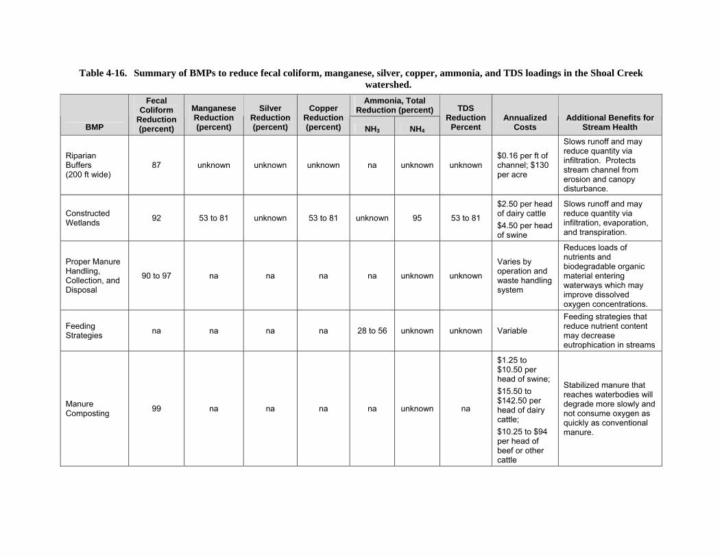
Table 4-16. Summary of BMPs to reduce fecal coliform, manganese, silver, copper, ammonia, and TDS loadings in the Shoal Creek watershed. Ammonia, Total
Reduction (percent)
BMP
Fecal Coliform
Reduction (percent)
Manganese Reduction (percent)
Silver Reduction (percent)
Copper Reduction (percent) NH3 NH4
TDS Reduction
Percent Annualized
Costs Additional Benefits for
Stream Health
Riparian Buffers (200 ft wide)
87 unknown unknown unknown na unknown unknown $0.16 per ft of channel; $130 per acre
Slows runoff and may reduce quantity via infiltration. Protects stream channel from erosion and canopy disturbance.
Constructed Wetlands 92 53 to 81 unknown 53 to 81 unknown 95 53 to 81
$2.50 per head of dairy cattle $4.50 per head of swine
Slows runoff and may reduce quantity via infiltration, evaporation, and transpiration.
Proper Manure Handling, Collection, and Disposal
90 to 97 na na na na unknown unknown
Varies by operation and waste handling system
Reduces loads of nutrients and biodegradable organic material entering waterways which may improve dissolved oxygen concentrations.
Feeding Strategies na na na na 28 to 56 unknown unknown Variable
Feeding strategies that reduce nutrient content may decrease eutrophication in streams
Manure Composting 99 na na na na unknown na
$1.25 to $10.50 per head of swine; $15.50 to $142.50 per head of dairy cattle; $10.25 to $94 per head of beef or other cattle
Stabilized manure that reaches waterbodies will degrade more slowly and not consume oxygen as quickly as conventional manure.

Table 4-16. Summary of BMPs to reduce fecal coliform, manganese, silver, copper, ammonia, and TDS loadings in the Shoal Creek watershed. Ammonia, Total
Reduction (percent)
BMP
Fecal Coliform
Reduction (percent)
Manganese Reduction (percent)
Silver Reduction (percent)
Copper Reduction (percent) NH3 NH4
TDS Reduction
Percent Annualized
Costs Additional Benefits for
Stream Health
Application of Composted Manure
na 68 68 68 na unknown 68
$1.25 to $10.50 per head of swine; $15.50 to $142.50 per head of dairy cattle; $10.25 to $94 per head of beef or other cattle
Application of composted manure improves soil infiltration and may reduce runoff volumes by 56 percent, potentially reducing rates of streambank erosion.
Alternative Watering Systems with Cattle Exclusion from Streams
29 to 46 unknown unknown unknown na unknown unknown
$5.50 to $9 per head of beef or other pastured cattle
Prevents streambank trampling and therefore decreases loads of manganese, silver, copper and TDS to the stream. Reduces direct deposition of manure into stream channel, which reduces ammonia and fecal coliform.
Grazing Land Management 40 to 90 unknown unknown unknown na unknown unknown
Variable – costs may be covered by fencing and alternative watering locations
Reduces soil erosion and associated metals

Illinois Environmental Protection Agency Shoal Creek Watershed TMDL Implementation Plan
40 Final Report
5.0 BMP PRIORITIZATION
This section discusses the pollutant sources in each of the impaired waterbodies, loads from those sources, and the various BMPs that could be used to reduce pollutant loads.
5.1 Shoal Creek Fecal coliform and manganese concentrations in Shoal Creek exceed Illinois’ water quality standards. The following sections discuss the various pollutant sources and BMPs to achieve the necessary load reductions.
5.1.1 Fecal Coliforms The Shoal Creek TMDL states that a 10 to 94 percent reduction in fecal coliform loading is needed to achieve water quality standards (depending on the flow condition). Wastewater treatment plants, onsite wastewater systems, and animal operations are likely the major anthropogenic sources of fecal coliforms to Shoal Creek.
Multiple BMPs are likely needed to achieve the fecal coliform water quality standard. Proper manure handling, collection, and disposal practices should be combined with composting manure, grazing land management, and/or alternative watering systems at animal operations located throughout the watershed. The following wastewater management practices are also suggested to meet the water quality standards in Shoal Creek: repairing or replacing failing onsite wastewater systems and disinfection of wastewater treatment plant effluent.
5.1.2 Manganese The Shoal Creek TMDL states that a 0 to 69 percent reduction in manganese loading is needed to achieve water quality standards (depending on the flow condition). Natural background loading and streambank erosion likely contribute some of this loading, but crop production, which tends to increase rates of erosion over large land areas, is likely the main contributor.
BMPs to reduce sediment loading (and associated manganese concentrations) are recommended for Shoal Creek. These potentially include riparian buffers, conservation tillage, cover crops, alternative watering sources, and grazing land management.
5.2 Cattle Creek Copper, ammonia, and TDS concentrations in Cattle Creek exceed Illinois’ water quality standards. The following sections discuss the various pollutant sources and BMPs to achieve the necessary load reductions.
5.2.1 Copper The copper TMDL for Cattle Creek stated that a 0 to 99 percent reduction in copper loading is needed to achieve water quality standards (depending on the flow condition). There are no point sources of copper in the watershed, and the potential nonpoint sources are poorly defined. It is suspected that copper containing fertilizers and/or sediment-bound copper are the anthropogenic sources in Cattle Creek. At this time, BMPs to reduce sediment erosion and runoff are recommended to reduce copper loads to Cattle Creek. These potentially include riparian buffers, conservation tillage, cover crops, alternative watering systems, and grazing land management.
5.2.2 Ammonia The ammonia TMDL for Cattle Creek stated that a 0 to 66 percent reduction in ammonia loading is needed to achieve water quality standards (depending on the flow condition). There are no point sources of ammonia in the watershed. Animal operations and septic systems are believed to be the two largest
Illinois Environmental Protection Agency Shoal Creek Watershed TMDL Implementation Plan
Final Report 41
sources of anthropogenic ammonia in the watershed. BMPs should be implemented to reduce loads from these two sources. Septic systems should be inspected and failing systems upgraded. Other potential BMPs include manure management, grazing land management, alternative watering systems, and riparian buffers.
5.2.3 Total Dissolved Solids The total dissolved solids (TDS) TMDL for Cattle Creek stated that a 0 to 39 percent reduction in TDS loading is needed to achieve water quality standards (depending on the flow condition). There are no point sources of TDS in the watershed. Potential nonpoint sources of TDS include feed lots, fertilizers, and crop production. Recommended BMPs include conservation tillage, cover crops, and riparian buffers.
5.3 Chicken Creek The TMDL for Chicken Creek stated that a 0 to 49 percent reduction in silver loading is needed to achieve water quality standards (depending on the flow condition). There are no point sources of silver in the watershed, and the potential nonpoint sources are poorly defined. It is suspected that sediment-bound silver is the major anthropogenic source in Chicken Creek. At this time, BMPs to reduce sediment erosion and runoff are recommended to reduce silver loads. These potentially include riparian buffers, conservation tillage, cover crops, alternative watering systems, and grazing land management.

Illinois Environmental Protection Agency Shoal Creek Watershed TMDL Implementation Plan
42 Final Report
6.0 MEASURING AND DOCUMENTING PROGRESS
Multiple agricultural BMPs will likely be needed to address the water quality impairments found in the Shoal Creek watershed. Water quality monitoring should be implemented to monitor BMP success, and to determine if additional BMPs are needed to achieve water quality standards. It may also be necessary to begin funding efforts for localized BMPs such as riparian buffer restoration. 7.0 REASONABLE ASSURANCE
USEPA requires reasonable assurance that TMDLs will be achieved and water quality standards will be met. For the Shoal Creek watershed, the primary strategy for attaining water quality standards is to implement agricultural BMPs and wastewater treatment plant effluent disinfection. However, landowner participation may be limited due to resistance to change and upfront costs. Educational efforts and cost sharing programs will likely increase participation to levels needed to protect water quality. The following sections discuss the programs that are available to assist landowners and local entities in implementing BMPs.
7.1 Environmental Quality Incentives Program (EQIP) Several cost share programs are available to landowners who voluntarily implement resource conservation practices in the Shoal Creek watershed. The most comprehensive is the NRCS Environmental Quality Incentives Program (EQIP) which offers cost sharing and incentives to farmers who utilize approved conservation practices to reduce pollutant loading from agricultural lands.
• The program will pay $10 for one year for each acre of farmland that is managed under a nutrient management plan (up to 400 acres per farm).
• Use of vegetated filter strips will earn the farmer $100/ac/yr for three years (up to 50 acres per farmer).
• The program will also pay 60 percent of the cost to construct grassed waterways, riparian buffers, and windbreaks.
• Use of residue management will earn the farmer $15/ac for three years (up to 400 acres per farm).
• Installation of drainage control structures on tile outlets will earn the farmer $5/ac/yr for three years for the effected drainage area as well as 60 percent of the cost of each structure.
• The program will pay 75 percent of the construction cost for a composting facility.
• Sixty percent of the fencing, controlled access points, spring and well development, pipeline, and watering facility costs are covered by the program.
• Waste storage facilities and covers for those facilities have a 50 percent cost share for construction.
• Prescribed grazing practices will earn the farmer $10/ac/yr for three years (up to 200 acres per farmer).
In order to participate in the EQIP cost share program, all BMPs must be constructed according to the specifications listed for each conservation practice.
The specifications and program information can be found online at: http://www.il.nrcs.usda.gov/programs/eqip/cspractices.html.

Illinois Environmental Protection Agency Shoal Creek Watershed TMDL Implementation Plan
Final Report 43
7.2 Conservation Reserve Program (CRP) The Farm Service Agency of the USDA supports the Conservation Reserve Program (CRP) which rents land that is converted from crop production to grass or forestland for the purposes of reducing erosion and protecting sensitive waters. This program is available to farmers who establish vegetated filter strips or grassed waterways. The program typically provides 50 percent of the upfront cost to establish vegetative cover and $185/ac/yr for up to 15 years.
More information about this program is available online at: http://www.nrcs.usda.gov/programs/crp/
7.3 Conservation 2000 In 1995 the Illinois General Assembly passed the Conservation 2000 bill providing $100 million in funding over a 6-year period for the promotion of conservation efforts. In 1999, legislation was passed to extend the program through 2009. Conservation 2000 currently funds several programs applicable to the Shoal Creek watershed through the Illinois Department of Agriculture.
General information concerning the Conservation 2000 Program can be found online at: http://www.agr.state.il.us/Environment/conserv/
7.3.1 Conservation Practices Program (CPP) The Conservation Practices Cost Share Program provides monetary incentives for conservation practices implemented on land eroding at one and one-half times or more the tolerable soil loss rate. Payments of up to 60 percent of initial costs are paid through the local conservation districts. Of the BMPs discussed in this plan, the program will cost share cover crops, filter strips, grassed waterways, no-till systems, and pasture planting. Other sediment control options such as contour farming and installation of stormwater ponds are also covered. Practices funded through this program must be maintained for at least 10 years.
More information concerning the Conservation Practices Program can be found online at: http://www.agr.state.il.us/Environment/conserv/
7.3.2 Streambank Stabilization Restoration Program Conservation 2000 also funds a streambank stabilization and restoration program aimed at restoring highly eroding streambanks. Research efforts are also funded to assess the effectiveness of vegetative and bioengineering techniques.
More information about this program is available online at: http://dnr.state.il.us/orep/c2000/grants/proginfo.asp?id=20
7.3.3 Sustainable Agriculture Grant Program (SARE) The Sustainable Agricultural Grant Program funds research, education, and outreach efforts for sustainable agricultural practices. Private landowners, organizations, educational, and governmental institutions are all eligible for participation in this program.
More information concerning the Sustainable Agricultural Grant Program can be found online at: http://www.sare.org/grants/

Illinois Environmental Protection Agency Shoal Creek Watershed TMDL Implementation Plan
44 Final Report
7.4 Nonpoint Source Management Program (NSMP) Illinois EPA receives federal funds through Section 319(h) of the Clean Water Act to help implement Illinois’ Nonpoint Source (NPS) Pollution Management Program. The purpose of the Program is to work cooperatively with local units of government and other organizations toward the mutual goal of protecting the quality of water in Illinois by controlling NPS pollution. The program emphasizes funding for implementing cost-effective corrective and preventative BMPs on a watershed scale; funding is also available for BMPs on a non-watershed scale and the development of information/education NPS pollution control programs.
The maximum federal funding available is 60 percent, with the remaining 40 percent coming from local match. The program period is two years unless otherwise approved. This is a reimbursement program.
Section 319(h) funds are awarded for the purpose of implementing approved NPS management projects. The funding will be directed toward activities that result in the implementation of appropriate BMPs for the control of NPS pollution or to enhance the public’s awareness of NPS pollution. Applications are accepted June 1 through August 1.
More information about this program is available online at: http://www.epa.state.il.us/water/financial-assistance/non-point.html
7.5 Agricultural Loan Program The Agricultural Loan Program offered through the Illinois State Treasury office provides low-interest loans to assist farmers who implement soil and water conservation practices. These loans will provide assistance for the construction, equipment, and maintenance costs that are not covered by cost share programs.
More information about this program is available online at: http://www.state.il.us/TREAS/ProgramsServices.aspx
7.6 Illinois Conservation and Climate Initiative (ICCI) The Illinois Conservation and Climate Initiative (ICCI) is a joint project of the State of Illinois and the Delta Pollution Prevention and Energy Efficiency (P2/E2) Center that allows farmers and landowners to earn carbon credits when they use conservation practices. These credits are then sold to companies or agencies that are committed to reducing their greenhouse gas emissions. Conservation tillage earns 0.5 metric tons (1.1 US ton) of carbon per acre per year (mt/ac/yr), grass plantings (applicable to filter strips and grassed waterways) earn 0.75 mt/ac/yr, and trees planted at a density of at least 250 stems per acre earn somewhere between 3.5 to 5.4 mt/ac/yr, depending on the species planted and age of the stand.
Carbon credits are currently selling at around $2.50 per mt. Current exchange rates are available online at http://chicagoclimatex.com. Administrative fees of $0.14/mt plus 8 percent are subtracted from the sale price.
Program enrollment occurs through the P2/E2 Center which can be found online at http://p2e2center.org/. The requirements of the program are verified by a third party before credits can be earned.
More information about carbon trading can be found online at: http://illinoisclimate.org/

Illinois Environmental Protection Agency Shoal Creek Watershed TMDL Implementation Plan
Final Report 45
7.7 Summary Tables 7-1 and 7-2 summarize the cost sharing programs available to Illinois landowners.
Table 7-1. Summary of Assistance Programs Available for Farmers in the Shoal Creek Watershed.
Assistance Program Program Description Contact Information
NSMP Provides grant funding for educational programs and implementation of nonpoint source pollution controls.
Illinois Environmental Protection Agency Bureau of Water Watershed Management Section, Nonpoint Source Unit P.O. Box 19276 Springfield, IL 62794-9276 Phone: (217) 782-3362
Agricultural Loan Program
Provides low-interest loans for the construction and implementation of agricultural BMPs. Loans apply to equipment purchase as well.
Office of State Treasurer Agricultural Loan Program 300 West Jefferson Springfield, Illinois 62702 Phone: (217) 782-2072 Fax: (217) 522-1217
NRCS EQIP Offers cost sharing and rental incentives to farmers statewide who utilize approved conservation practices to reduce pollutant loading from agricultural lands. Applies to nutrient management plans, filter strips, grassed waterways, riparian buffers, and conservation tillage.
FSA CRP Offsets income losses due to land conversion by rental agreements. Targets highly erodible land or land near sensitive waters. Provides up to 50 percent of the upfront cost to establish vegetative cover and $185/ac/yr for up to 15 years for converted land.
Conservation 2000 CPP
Provides up to 60 percent cost share for several agricultural BMPs: cover crops, filter strips, grassed waterways.
Conservation 2000 Streambank Stabilization Restoration Program
Provides 75 percent cost share for establishment of riparian corridors along severely eroding stream banks. Also provides technical assistance and educational information for interested parties.
SARE Funds educational programs for farmers concerning sustainable agricultural practices.
Local SWCD Provides incentives for individual components of nutrient management planning, use of strip tillage, and restoration of riparian buffers.
ICCI Allows farmers to earn carbon trading credits for use of conservation tillage, grass, and tree plantings.
Jackson County SWCD 1213 N 14th St Murphysboro, IL 62966-2950 Phone: (618) 684-3471 Fax: (618) 684-3980

Illinois Environmental Protection Agency Shoal Creek Watershed TMDL Implementation Plan
46 Final Report
Table 7-2. Assistance Programs Available for Agricultural BMPs.
BMP Cost Share Programs and Incentives
Education and Outreach Conservation 2000 Streambank Stabilization Restoration Program SARE NSMP Local SWCD ULWREP
Nutrient Management Plan EQIP: $10/ac for one year, 400 ac. max. Local SWCD: up to $30/ac for one year ULWREP: contact agency for individual resource allocations
Conservation Tillage EQIP: $15/ac for three years, 400 ac. max. ICCI: earns 0.5 mt/ac/yr of carbon trading credit ULWREP: contact agency for individual resource allocations
Cover Crops CPP: cost share of 60 percent ULWREP: contact agency for individual resource allocations
Filter Strips EQIP: $100/ac for three years, 50 ac. max. CPP: 60 percent of construction costs CRP: 50 percent of the upfront cost to establish vegetative cover and $185/ac/yr for up to 15 years ICCI: earns 0.75 mt/ac/yr of carbon trading credit for each acre planted
Grassed Waterways EQIP: 60 percent of construction costs CPP: 60 percent of construction costs CRP: 50 percent of the upfront cost to establish vegetative cover and $185/ac/yr for up to 15 years ICCI: earns 0.75 mt/ac/yr of carbon trading credit for each acre planted
Land Retirement of Highly Erodible Land or Land Near Sensitive Waters
CRP: 50 percent of the costs of establishing vegetative cover and cash incentive of $185/ac/yr for 15 years ICCI: earn between 0.75 and 5.4 mt/ac/yr of carbon trading credit depending on species planted ULWREP: contact agency for individual resource allocations
Restoration of Riparian Buffers EQIP: 60 percent of construction of costs CRP: 50 percent of the costs of establishing vegetative cover and cash incentive of $185/ac/yr for 15 years ICCI: earn between 0.75 and 5.4 mt/ac/yr of carbon trading credit depending on species planted ULWREP: contact agency for individual resource allocations
Note: Cumulative cost shares from multiple programs will not exceed 100 percent of the cost of construction.

Illinois Environmental Protection Agency Shoal Creek Watershed TMDL Implementation Plan
Final Report 47
8.0 IMPLEMENTATION TIMELINE
This implementation plan for the Shoal Creek watershed defines a phased approach for achieving the water quality standards (Figure 8-1). Ideally, implementing control measures on nonpoint sources will be based on voluntary participation which will depend on 1) the effectiveness of the educational programs for farmers, landowners, and owners of onsite wastewater systems, and 2) the level of participation in the programs. In addition, point source dischargers operating under a disinfection exemption are required to comply with the geometric mean fecal coliform water quality standard of 200 cfu/100 mL at the closest point downstream where recreational use occurs in the receiving water or where the water flows into a fecal-impaired segment. Facilities with year-round disinfection exemptions may be required to provide the Agency with updated information to demonstrate compliance with these requirements. Facilities directly discharging into a fecal-impaired segment may have their year-round disinfection exemption revoked through future NPDES permitting actions. This section outlines a schedule for implementing the control measures and determining whether or not they are sufficient to meet the water quality standards.
Phase I of this implementation plan should focus on education of farm owners concerning the benefits of agricultural BMPs on crop yield, soil quality, and water quality as well as cost share programs available in the watershed. It is expected that initial education through public meetings, mass mailings, TV and radio announcements, and newspaper articles could be achieved in less than 6 months. As described in Section 7.0., assistance with educational programs is available through the following agencies: the Illinois Department of Agriculture Conservation 2000 Streambank Stabilization Restoration Program, the Illinois Department of Agriculture Sustainable Agriculture Grant Program (SARE), the Illinois Environmental Protection Agency Nonpoint Source Management Program (NSMP), and the local Soil and Water Conservation Districts. During this phase, the sewage treatment plants may be asked to submit fecal coliform data to IEPA to determine if a disinfection exemption is still appropriate.
Phase II of the implementation schedule will involve voluntary participation of landowners in BMPs such as proper management of manure and fertilizers, grazing land management, and use of filter strips, composting, constructed wetlands, conservation tillage, cattle exclusion from streams, and grassed waterways. The local Natural Resources Conservation Service office will be able to provide technical assistance and cost share information for these BMPs. In addition, initial inspections of all onsite wastewater treatment systems and necessary repairs may begin. Continued monitoring of water quality in the watershed should continue throughout this phase, which will likely take one to three years.
If pollutant concentrations measured during Phase II monitoring remain above the water quality standards, Phase III of the implementation plan will be necessary. The load reduction achieved during Phase II should be estimated by 1) summarizing the areas where BMPs are in use, 2) calculating the reductions in loading from BMPs, and 3) determining the impacts on pollutant concentrations measured before and after Phase II implementation. If BMPs are resulting in decreased concentrations, and additional areas could be incorporated, further efforts to include more stakeholders in the voluntary program will be needed. If the Phase II BMPs are not having the desired impacts on pollutant concentrations, or additional areas of incorporation are not available, supplemental BMPs, such as restoration of riparian areas and stream channels will be needed. In addition, sewage treatment plants may be required to add disinfection processes if fecal coliform standards in receiving and downstream segments are not being met. If required, this phase may last five to ten years.
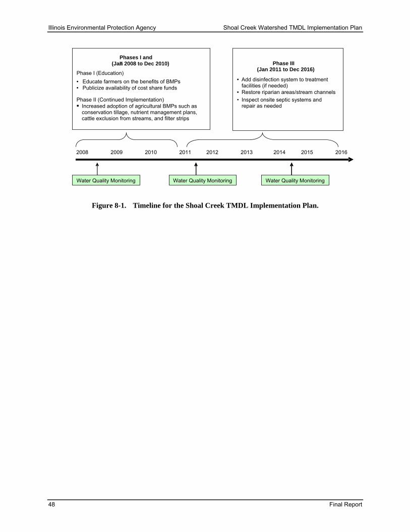
Illinois Environmental Protection Agency Shoal Creek Watershed TMDL Implementation Plan
48 Final Report
Figure 8-1. Timeline for the Shoal Creek TMDL Implementation Plan.
2008 2009 2010 2011 2012 2013 2014 2015 2016
Phases I and II (Jan 2008 to Dec 2010)
Phase I (Education) • Educate farmers on the benefits of BMPs• Publicize availability of cost share funds
Phase II (Continued Implementation) Increased adoption of agricultural BMPs such as conservation tillage, nutrient management plans, cattle exclusion from streams, and filter strips
Phase III (Jan 2011 to Dec 2016)
• Add disinfection system to treatment facilities (if needed)
• Restore riparian areas/stream channelsInspect onsite septic systems and repair as needed
• •
•
••
Water Quality MonitoringWater Quality Monitoring Water Quality Monitoring

Illinois Environmental Protection Agency Shoal Creek Watershed TMDL Implementation Plan
Final Report 49
9.0 CONCLUSIONS
Animal operations, failing onsite sewage treatment systems, and sewage treatment plants that operate under disinfection exemption are considered the most likely sources of fecal coliform in Shoal Creek. Ammonia exceedances in Cattle Creek are likely due to animal operations and septic systems. All of the other water quality exceedances (i.e., manganese in Shoal Creek, silver in Chicken Creek, and total dissolved solids and copper in Cattle Creek) are likely due to sediment erosion and delivery.
The implementation of BMPs in the Shoal Creek watershed should occur in a phased approach. Phase I of this implementation plan should provide education and financial incentives to farmers in the watershed to encourage the use of BMPs. Phase II should occur during and following Phase I and should involve voluntary participation of farmers in the watershed, and submittal of fecal coliform data for the wastewater treatment plants in the watershed. Future water quality monitoring will determine whether or not these BMPs are capable of achieving water quality standards.
Whether or not Phase III will be required depends on the results of future water quality sampling. If the water quality standards are not being met after implementation of the Phase II BMPs, then regional BMPs (such as restoration of stream channels and riparian areas) may be needed. Additional wastewater treatment plant upgrades may also be considered.
As BMPs are implemented, water quality in the watershed should improve accordingly. Measuring the effectiveness of these BMPs will require continued sampling of water quality over the next several years.

Illinois Environmental Protection Agency Shoal Creek Watershed TMDL Implementation Plan
50 Final Report
10.0 REFERENCES
Al-Kaisi, M., M. Hanna, and M. Tidman. 2000. Survey: Iowa No-till Holds Steady. Integrated Crop Management, IC-484(23), October 23, 2000.
ASAE. 1998. ASAE Standards, 45th edition: Standards, Engineering Practices, Data. St. Joseph, MI. American Society of Agricultural Engineers.
Buman, R.A., B.A. Alesii, J.L. Hatfield, and D.L. Karlen. 2004. Profit, yield, and soil quality effects of tillage systems in corn - soybean rotations, Journal of Soil and Water Conservation, Vol.59, No. 6.
CCSWCD. 2003. Homer Lake Application for Section 319(h) Financial Assistance. Submitted to Illinois Environmental Protection Agency Division of Water Pollution Control. Submitted by Champaign County Soil and Water Conservation District in cooperation with the Champaign County Forest Preserve District, July 31, 2003.
CIAS. 1996. Windrow composting systems can be feasible, cost-effective. University of Wisconsin, Center for Integrated Agricultural Systems, Research Brief # 20.
Czapar, G.F., J.M. Laflen, G.F. McIsaac, D.P. McKenna. 2006. Effects of Erosion Control Practices on Nutrient Loss, University of Illinois.
Davis, J. G., and A. M. Swinker. 2004. Horse Manure Management. Colorado State Cooperative Extension.
Dillaha, T.A., Renear, R.B., Mostaghimi, S. and Lee, D. 1989. "Vegetative Filter Strips for Agricultural Nonpoint Source Pollution Control." Transactions of the American Society of Agricultural Engineers, 32(2):513-519.
Ebelhar, S.A. and M. P. Plumer. 2007. Annual Ryegrass Varieties for Southern Illinois. University of Illinois Department of Crop Sciences.
Goo, R. 2004. Do’s and Don’ts Around the Home. U.S. Environmental Protection Agency, Nonpoint Source Control Branch.
Government of Alberta. 2007. Beneficial Management Practice Evaluation in the Battersea Drain and Lower Little Bow River Watersheds.
Hajjar, L.M. 2000. Final Report for Section 309 – Cumulative and Secondary Impacts Task 2 – Model Septic System Maintenance Program. Office of Ocean and Coastal Resource Management South Carolina Department of Health and Environmental Control.
Harman, W.L., T. Gerik, H.A. Torbert III, K.N. Potter. 2003. Agronomic and economic implications of conservation tillage and ultra-narrow row cropping systems. National Conservation Tillage Cotton and Rice Conference Proceedings. Jan. 23-24, Houston, TX. p. 11-13.
HRWCI. 2005. Agricultural Phosphorus Management and Water Quality in the Midwest. Heartland Regional Water Coordination Initiative. Iowa State University, Kansas State University, the University of Missouri, the University of Nebraska–Lincoln and the USDA Cooperative State Research, Education and Extension Service.
IAH. 2002. Illinois Agronomy Handbook, 23rd Edition. University of Illinois Extension, College of Agricultural, Consumer, and Environmental Sciences.
IEPA. 2006. Illinois Integrated Water Quality Report and Section 303(D) List – 2006. Illinois Environmental Protection Agency – Bureau of Water. IEPA/BOW/06-002. Available online at http://www.epa.state.il.us/water/tmdl/303d-list.html.

Illinois Environmental Protection Agency Shoal Creek Watershed TMDL Implementation Plan
Final Report 51
IEPA. 2007. TMDL Development for the Shoal Creek Watershed, Illinois. Illinois Environmental Protection Agency – Bureau of Water. Springfield, Illinois.
IEPA. 2007b. Shoal Creek Watershed TMDL Stage One. Illinois Environmental Protection Agency – Bureau of Water. Springfield, Illinois.
Iowa State University. 2005. Estimated Costs for Livestock Fencing. Iowa State University Extension. FM1855. Revised July 2005.
Kalita, Prasanta. 2000. Vegetative Filter Strips to Reduce Pathogens and Nutrients in Runoff from Livestock Feedlots. Department of Crop Sciences College of Agriculture, Consumer and Environmental Sciences, University of Illinois Extension.
Larney, F. J., L.J. Yanke, J.J. Miller, and T.A. McAllister. 2003. Fate of Coliform Bacteria in Composted Beef Cattle Feedlot Manure. Journal of Environmental Quality. 32:1508 1515 (2003).
Lewandrowski, J., M. Peters, C. Jones, R. House, M. Sperow, M. Eve, and K. Paustian. 2004. Economics of Sequestering Carbon in the U.S. Agricultural Sector, Technical Bulletin No. (TB1909) 69 pp, United States Department of Agriculture, Economic Research Service.
Mannering, J.V., D.R. Griffith, and K.D. Johnson. 1998. Winter Cover Crops – Their Value and Management. Department of Agriculture, Purdue University, Cooperative Extension Service, Publication AY-247.
Marsh, L. 2001. Pumping Water from Remote Locations for Livestock Watering. Virginia Tech Cooperative Extension, Publication Number 442-755.
Meals, D.W. and D.C. Braun. 2006. Demonstration of Methods to Reduce E. coli Runoff from Dairy Manure Application Sites. J Environ Qual 35:1088-1100. American Society of Agronomy, Crop Science Society of America, and Soil Science Society of America.
NCDENR. 2005. Updated Draft Manual of Stormwater Best Management Practices. North Carolina Department of Environment and Natural Resources, Division of Water Quality.
NCEEP. 2004. North Carolina Ecosystem Enhancement Program Annual Report 2003-2004. North Carolina Department of Environment and Natural Resources.
NCSU. 2002. Riparian Buffers and Controlled Drainage to Reduce Agricultural Nonpoint Source Pollution. Departments of Soil Science and Biological and Agricultural Engineering, North Carolina Agricultural Research Service, North Carolina State University, Raleigh, North Carolina. Technical Bulletin 318, September 2002.
NRCS. 2002a. Natural Resources Conservation Service Conservation Practice Standard Field Border (Feet) Code 386.
NRCS. 2002b. Natural Resources Conservation Service Conservation Practice Standard Constructed Wetland (Feet) Code 656. United States Department of Agriculture, Natural Resources Conservation Service.
NRCS. 2003. Costs Associated With Development and Implementation of Comprehensive Nutrient Management Plans Part I—Nutrient Management, Land Treatment, Manure and Wastewater Handling and Storage, and Recordkeeping. United States Department of Agriculture, Natural Resources Conservation Service.
NSFC. 1998. Ultraviolet Disinfection. National Small Flows Clearinghouse. Project funded by U.S. Environmental Protection Agency, Fact Sheet WWFSOM20.
Olson, K.D. and N.B. Senjem. 2002. Economic Comparison of Incremental Changes in Till Systems in the Minnesota River Basin, University of Minnesota, 2002.

Illinois Environmental Protection Agency Shoal Creek Watershed TMDL Implementation Plan
52 Final Report
OSUE. 1990. Hairy Vetch as an Ohio Cover Crop. Ohio State University Extension Food, Agricultural and Biological Engineering. Fact Sheet AGF-006-90.
OSUE. 1994. Vegetative Filter Strips: Application, Installation and Maintenance. Ohio State University Extension Food, Agricultural and Biological Engineering. Fact Sheet AEX-467-94.
OSUE. 1999. Cover Crop Fundamentals. Ohio State University Extension Food, Agricultural and Biological Engineering. Fact Sheet AGF-142-99.
PSU. 2005. Composting for Small Scale Livestock Operations. Pennsylvania Nutrient Management Program. Pennsylvania State University.
Rouge River. 2001. Planning and Cost Estimating Criteria for Best Management Practices (Update). Rouge River National Wet Weather Demonstration Project, Wayne County, Michigan. April 2001. TR-NPS25.00.
Sample, Trevor. 2007. Comments Concerning Drafts of Homer Lake Implementation Plan. Champaign County Soil and Water Conservation District.
Tetra Tech. 2006. Lake Maumelle Watershed Management Plan. Prepared for Board of Commissioners Central Arkansas Water, October 2006, draft.
UME. 1996. Tillage Best Management Practices for Corn-Soybean Rotations in the Minnesota River Basin, University of Minnesota Extension, FO-06676.
University of Alberta. 2000. Manure Management – Benefits of Compost & Processing.
University of Missouri. 1993. How to Build a Compost Bin. University of Missouri Extension.
USDA. 1999. CORE4 Conservation Practices Training Guide The Common Sense Approach to Natural Resource Conservation. United States Department of Agriculture, Natural Resources Conservation Service.
USDA. 2003. Agricultural Phosphorus and Eutrophication Second Edition. United States Department of Agriculture, Agricultural Research Service ARS–149 September 2003.
USEPA. 1999a. Preliminary Data Summary: Feedlots Point Source Category Study. EPA-821-R-99-002. January 1999.
USEPA. 1999b. Wastewater Technology Fact Sheet Chlorine Disinfection. U.S. Environmental Protection Agency, EPA 832-F-99-062, September 1999.
USEPA. 1999c. Wastewater Technology Fact Sheet Ozone Disinfection. U.S. Environmental Protection Agency, EPA 832-F-99-063, September 1999.
USEPA. 2001. Alternative Technologies/Uses for Manure. U.S. Environmental Protection Agency, Office of Wastewater Management.
USEPA. 2002a. Development Document for the Final Revisions to the National Pollutant Discharge Elimination System Regulation and the Effluent Guidelines for Concentrated Animal Feeding Operations. EPA-821-R-03-001. December 2002.
USEPA. 2002b. Onsite Wastewater Treatment Systems Manual. EPA/625/R-00/008. February 2002.
USEPA. 2002c. Post-Construction Storm Water Management in New Development & Redevelopment. U.S. Environmental Protection Agency, Office of Wastewater Management.
USEPA. 2003. National Management Measures to Control Nonpoint Source Pollution from Agriculture. EPA 841-B-03-004, July 2003.

Illinois Environmental Protection Agency Shoal Creek Watershed TMDL Implementation Plan
Final Report 53
Weiss, P.T., J.S. Gulliver, and A.J. Erickson. 2007. Cost and Pollutant Removal of Stormwater Treatment Practices. Journal of Water Resources Planning and Management, ASCE, May-June 2007, 133:3 (218).
Wenger, S. 1999. A Review of the Scientific Literature on Riparian Buffer Width, Extent, and Vegetation. for the Office of Public Service & Outreach Institute of Ecology, University of Georgia, Revised Version March 5, 1999.
Winer, R. 2000. National Pollutant Removal Performance Database for Stormwater Treatment Practices, 2nd Edition. Center for Watershed Protection. Ellicott City, MD.
Woerner, B. and J. Lorimer. 2006. Alternative Treatments to Minimize Water Pollution from Open Animal Feedlots. Department of Ag and Bio Systems Engineering, Iowa State University.
Wossink, A., and D. Osmond. 2001. Cost and Benefits of Best Management Practices to Control Nitrogen.