Long Run and Short Effects in Static PanelModels

Peter Egger and Michael Pfaffermayr∗

January 28, 2002

Abstract

For short and fat panels the Mundlak model can be viewed asan approximation of a general dynamic autoregressive distributed lagmodel. We give an exact interpretation of short run and long effectsand provide simulations to assess the quality of the approximation ofthe long run and short run effects by the parameters of the MundlakModel.Key words: Random Effects Models, Mundlak Model, Panel

Econometrics.JEL classification:

∗Affiliation of both authors: Department of Economic Theory, Economic Poliy and

Economic History, University of Innsbruck, Universitätsstr. 15, A-6020 Innsbruck, Austria

and Austrian Institute of Economic Research, PO-Box 91, A-1103-Vienna, Austria, E-mail:

Peter.Egger@uibk.ac.at and Michael.Pfaffermayr@uibk.ac.at.

1

1 Introduction1

Since the seminal work of Kuh (1959) and Houthakker (1965) it is argued that

in static panel models the long run effects are mainly captured by between

estimates, while the within estimates represent short-run effects.

Baltagi and Griffin (1984) investigate the case of underspecified lag dy-

namics in a finite distributed lag error components model. They conclude

that ”the OLS estimator provides a robust estimator of the long run ... elas-

ticity under alternative degrees of misspecification, variance components, and

time series observations. In contrast, the within estimator offers a good es-

timator of the short run effects but can severely underestimate the long run

response.” (ibid, p. 643)

Pirotte (1999) assumes a general dynamic error components model as the

data generating process and investigates whether the within and between es-

timates approximate the short and long run effects properly. From his Monte

Carlo simulations he concludes that ”the probability limit of the Between es-

timator of the static model converges, in all cases, to long run effects” and

that ”long run effects are obtained directly from the static relation without

the need of a dynamic model” (p. 155).

In many applications, data comprise a panel with a large cross-section

dimension, but only a few observations over time. In such short and fat

panels, it is impossible to estimate complex dynamic models and it is im-

portant to investigate, whether and under which circumstances static panel

models provide a reasonable approximation of the short run and the long

1We are grateful to Sylvia Kaufmann and Andrea Weber for helpful comments.

2

run effects. The present paper follows Pirotte (1999) in assuming a dynamic

error components model as the data generating process (more precisely an

autoregressive distributed lag model ADL(1,1)). In contrast to previous re-

search, we demonstrate that disregarding the dynamic process (the lagged

endogenous variable) results in an approximation error and in autocorrelated

residuals. Noteworthy, the former does not vanish in large cross-sections,

which has been suggested in Pirotte (1999). We derive the probability limit

of the approximation error of both the short run and the long run param-

eter estimate. Moreover, we assess the determinants of this approximation

bias and its small sample properties in a Monte Carlo experiment. Specifi-

cally, we demonstrate that both the short run and the long run parameter

are underestimated and this approximation bias is the larger, the slower the

adjustment of the dependent variable (i.e. the higher the omitted parameter

of the lagged dependent variable) and the shorter the time dimension of the

panel.

The next section discusses the within and between estimates on the basis

of the Mundlak (1978) model, which seems to be the natural specification

in this case, and evaluates the corresponding approximation biases. Sec-

tion 3 reports the results of the Monte Carlo simulations. The last section

summarizes the main findings.

2 The basic model and the approximation bias

Mundlak’s (1978) model can be interpreted as an approximation to an ADL(1,1)

model (or ADL-models in general), providing both long run and short run

3

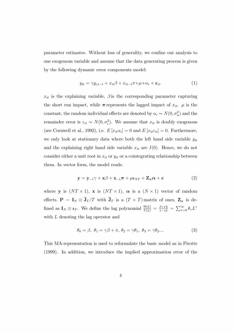
parameter estimates. Without loss of generality, we confine our analysis to

one exogenous variable and assume that the data generating process is given

by the following dynamic error components model:

yit = γyi,t−1 + xitβ + xit−1π+µ+αi + εit. (1)

xit is the explaining variable, β is the corresponding parameter capturing

the short run impact, while π represents the lagged impact of xit. µ is the

constant, the random individual effects are denoted by αi ∼ N(0, σ2α) and the

remainder error is εit ∼ N(0,σ2²). We assume that xit is doubly exogenous

(see Cornwell et al., 1992), i.e. E [xitαi] = 0 and E [xitεit] = 0. Furthermore,

we only look at stationary data where both the left hand side variable yit

and the explaining right hand side variable xit are I(0). Hence, we do not

consider either a unit root in xit or yit or a cointegrating relationship between

them. In vector form, the model reads:

y = y−1γ + xβ + x−1π + µιNT + Zαα+ ε (2)

where y is (NT × 1), x is (NT × 1), α is a (N × 1) vector of randomeffects. P = IN ⊗ JT/T with JT is a (T × T )matrix of ones, Zα is de-

fined as IN ⊗ ιT . We define the lag polynomial Θ(L)Γ(L)

= β+πL1−γL =

P∞τ=0 θτL

τ

with L denoting the lag operator and

θ0 = β, θ1 = γβ + π, θ2 = γθ1, θ3 = γθ2.... (3)

This MA-representation is used to reformulate the basic model as in Pirotte

(1999). In addition, we introduce the implied approximation error of the

4

static error components model.

yit =Θ (L)

Γ (L)xit +

µ+ αi + εitΓ (L)

(4)

= xitβ +1

1− γxi (γβ + π) +

∞Xj=0

γj (xit−j−1 − xi) (γβ + π)

+µ

1− γ+

αi1− γ

+ uit

= xitβ + xieϕ+ ∞Xj=0

γj (xit−j−1 − xi) (γβ + π) + eµ+ eαi + uitwhere eϕ = 1

1−γ (γβ + π) , eµ = µ1−γ , eαi = αi

1−γ . The transformation with the

lag polynomial Γ (L) furthermore implies that the error term is now AR(1)

and given by uit = γuit−1 + εit (see Greene, 1993) with σ2u =σ2ε1−γ2 . We as-

sume an infinite history of the explaining variable, so that the approximation

error becomesP∞

j=0 γj (xit−j−1 − xi) (γβ + π). It can immediately be seen

that this term vanishes, if γ = 0 and the underlying model reduces to that

analyzed in Baltagi and Griffin (1984). Therefore, in the absence of a lagged

dependent variable the Mundlak model is a perfect representation of a model

with lagged exogenous variables, and the underspecified lag dynamics is fully

compensated by the inclusion of the group mean as a control.

In contrast to Baltagi and Griffin (1984), Pirotte (1999), and others we

do not consider a dynamic data generating process for the right hand side

variable xit, rather in both the theoretical analysis and the simulation exercise

we assume that the xit is IID, namely xit = µζ i + ηit with µ ∈ R, ζ i ∼N¡0, σ2ζ

¢, ηit ∼ N

¡0, σ2η

¢, E [ζ iηit] = 0.

Applying the within transformation Q = I−P to the Mundlak approxi-

5

mation, one gets

Qy = Qxβ+QPxeϕ+ ∞Xj=0

γjQ (x−j−1 −Px) (γβ + π) +QZα eα+Qu= Qxβ +

∞Xj=0

γjQx−j−1 (γβ + π) +Qu, (5)

where x−j−1 is (NT × 1) and includes the elements (xi1−j−1, xi2−j−1,..., xiT−j−1)0.This approximation produces an omitted variable bias, which for fixed T and

an infinite history of xit is given by

p limN→∞

hbβWithin − βi= p lim

N→∞

" ∞Xj=0

γj(x0Qx)−1x

0Qx−j−1 (γβ + π)

#, (6)

since p limN→∞£x0Qu¤= 0, because xit is exogenous and uncorrelated with

the error term. For j < T − t, it follows that

p limN→∞

[

Ãxit − 1

T

TXτ=1

xiτ

!Ãxit−j−1 − 1

T

TXτ=1

xiτ−j−1

!] = (7)

p limN→∞

[xitxit−j−1 − xit 1T

TXτ=1

xiτ−j−1 − xit−j−1 1T

TXτ=1

xiτ

+1

T 2

TXτ=1

TXτ 0=1

xiτxiτ 0−j−1] =

µ2σ2ζ − 2µ2σ2ζ −2

Tσ2η + µ

2σ2ζ +T − j − 1T 2

σ2η = −T + j + 1

T 2σ2η,

while it is zero otherwise (j ≥ T − t). Furthermore,

p limN→∞

[

Ãxit − 1

T

TXτ=1

xiτ

!Ãxit − 1

T

TXτ=1

xiτ

!] = (8)

µ2σ2ζ + σ2η − 2µ2σ2ζ −2

Tσ2η + µ

2σ2ζ +1

Tσ2η =

T − 1T

σ2η,

6

Combining these two results, the probability limit of the approximation bias

of the short run parameter (after within transformation) amounts to

p limN→∞

"T−1Xj=0

γj(x0Qx)−1x

0Qx−j−1

#(γβ + π) = (9)

T−1Xj=0

γjp limN→∞

³(x

0Qx)−1

´· p lim

N→∞

³x0Qx−j−1

´(γβ + π) =

−T−1Xj=0

γjµT + j + 1

T (T − 1)¶(γβ + π) < 0.

For large N and fixed T , the within estimate tends to underestimate the

true short run impact, especially, in short panels (small T ) and with a high

persistence parameter γ. However, it can immediately be seen that the bias

vanishes, if T approaches infinity and as long as γ < 1.2

The long run impact of the explaining variable can be calculated from

the between transformation, since

E (y)|xit=xit−1=x =β + π

1− γx (10)

and

Py = Pxβ+Pxeϕ+ ∞Xj=0

γjP (x−j−1 −Px) (γβ + π) +PZα eα+Pu. (11)

The corresponding approximation bias of the long run impact is

p limN→∞

hbβ + beϕ− β − eϕi = (12)

p limN→∞

" ∞Xj=0

γjh(x

0Px)−1x

0Px−j−1 − I

i(γβ + π)

#,

2 limT→∞PT−1j=0 γj

³T+j+1T (T−1)

´(γβ + π) < (γβ + π) limT→∞

h³2T+1T (T−1)

´PT−1j=0 γj

i=

(γβ + π) limT→∞³

2T+1T (T−1)

´limT→∞

PT−1j=0 γj = 0, since limT→∞

³2T+1T (T−1)

´= 0.

7

since in addition to p limN→∞£x0Qu¤= 0, p limN→∞

£x0PZα eα¤ = 0holds

by assumption. For j < T − 1, one obtains

p limN→∞

"Ã1

T

TXτ=1

xiτ

!Ã1

T

TXτ=1

xiτ−j−1

!#= µ2σ2ζ +

T − j − 1T 2

σ2η,

while for j ≥ T − 1 we have

p limN→∞

"Ã1

T

TXτ=1

xiτ

!Ã1

T

TXτ=1

xiτ−j−1

!#= µ2σ2ζ . (13)

Combining terms yields

p limN→∞

" ∞Xj=0

γjh(x

0Px)−1x

0Px−j−1 − I

i(γβ + π)

#= (14)"

−T−2Xj=0

γj

Ã(j + 1)σ2η

T (Tµ2σ2ζ + σ2η)

!−

∞Xj=T−1

γj

Ãσ2η

Tµ2σ2ζ + σ2η

!#(γβ + π) < 0.

It is evident that in absolute terms the approximation bias of the between

estimate shrinks, if T grows large, if the persistence parameter γ becomes

smaller or if the between variation in the right hand side variable (σ2ζ) is high

or becomes more and more important (µ increases). This bias of the long

run estimate likewise tends to zero as T approaches infinity for γ < 1.3

The Mundlak model integrates both approaches in an error components

framework. Transforming the data according to Fuller and Battese (1973) by

σεΩ−1/2 = Q+ σε

σ1P, σ1 =

pTσ2α + σ2ε gives the well known Mundlak (1978)

3It suffices to show that limT→∞PT−2j=0 γj

³(j+1)σ2η

T (Tµ2σ2ζ+σ2η)

´= 0. An upper bound is given

by limT→∞PT−2j=0 γj

³(T+1)σ2η

T (Tµ2σ2ζ+σ2η)

´= limT→∞

³(T+1)σ2η

T (Tµ2σ2ζ+σ2η)

´limT→∞

PT−2j=0 γj = 0.

8

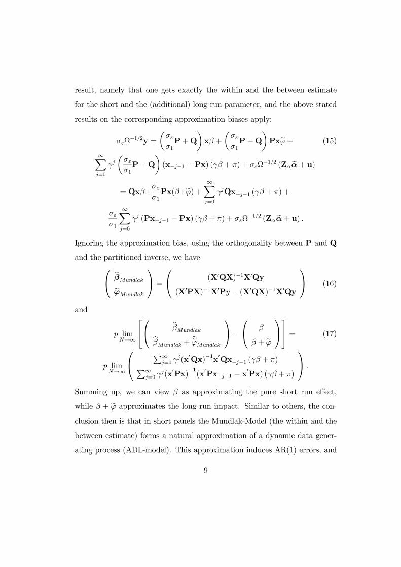
result, namely that one gets exactly the within and the between estimate

for the short and the (additional) long run parameter, and the above stated

results on the corresponding approximation biases apply:

σεΩ−1/2y =

µσε

σ1P+Q

¶xβ +

µσε

σ1P+Q

¶Pxeϕ+ (15)

∞Xj=0

γjµσε

σ1P+Q

¶(x−j−1 −Px) (γβ + π) + σεΩ

−1/2 (Zα eα+ u)= Qxβ+

σε

σ1Px(β+eϕ) + ∞X

j=0

γjQx−j−1 (γβ + π) +

σε

σ1

∞Xj=0

γj (Px−j−1 −Px) (γβ + π) + σεΩ−1/2 (Zα eα+ u) .

Ignoring the approximation bias, using the orthogonality between P and Q

and the partitioned inverse, we have bβMundlakeϕMundlak =

(X0QX)−1X0Qy

(X0PX)−1X0Py − (X0QX)−1X0Qy

(16)

and

p limN→∞

bβMundlakbβMundlak + beϕMundlak−

β

β + eϕ = (17)

p limN→∞

P∞j=0 γ

j(x0Qx)−1x

0Qx−j−1 (γβ + π)P∞

j=0 γj(x

0Px)

−1(x

0Px−j−1 − x0Px) (γβ + π)

.Summing up, we can view β as approximating the pure short run effect,

while β + eϕ approximates the long run impact. Similar to others, the con-clusion then is that in short panels the Mundlak-Model (the within and the

between estimate) forms a natural approximation of a dynamic data gener-

ating process (ADL-model). This approximation induces AR(1) errors, and

9

estimating an AR(1) model in the spirit of Baltagi and Li (1991), besides

improving efficiency, provides some valuable information on the extent of

the approximation bias, since it gives a direct (though in small samples not

necessarily consistent) estimate of γ.

Another observation is that the familiar Hausman (1978) test may lead

to a rejection of the static random effects model even if the ”true” model is

a dynamic random effects one (i.e. π = 0, γ > 0). The reason is that the

approximation induces correlation between the explaining variable and the

individual random effect due to the omission of the long run effect. Hence,

the rejection of a test of eϕMundlak = 0 can have three reasons. (i) beϕ 6= 0

although γ = 0 and π = 0 (no dynamics), which is the traditional Hausman

(1978) and Mundlak (1978) result of testing E [xiα] = 0. E [xiα] = 0, but

the true eϕ 6= 0 because of omitting a relevant long run impact with (ii) π 6= 0and/or γ > 0 or (iii) π = 0 and γ > 0. To our knowledge, the latter two

reasons have not been considered before.

3 Simulation Results

Our Monte Carlo simulation set-up compares four model parameters to as-

sess the sensitivity of four different estimators: the error components model

(Amemiya, 1971, type), which ignores the long run effects, the Mundlak

model, which obtains both the within estimates and the between estimates,

the error components AR(1) model and the Mundlak AR(1) model using the

autocorrelation correction proposed by Baltagi and Li (1991).4 We assume

4In the Mundlak AR(1) model, the group means do not represent pseudo averages over

time. This results in slight deviations of the estimated between error component from its

10

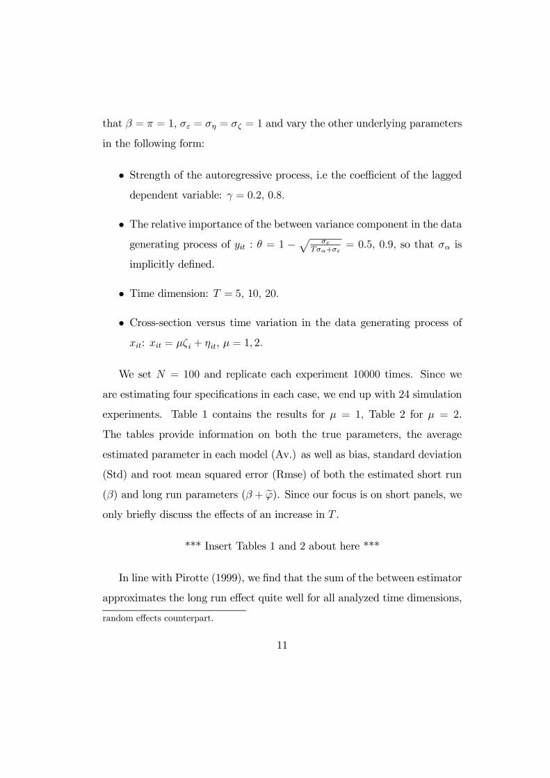
that β = π = 1, σε = ση = σζ = 1 and vary the other underlying parameters

in the following form:

• Strength of the autoregressive process, i.e the coefficient of the laggeddependent variable: γ = 0.2, 0.8.

• The relative importance of the between variance component in the datagenerating process of yit : θ = 1 −

p σεTσα+σε

= 0.5, 0.9, so that σα is

implicitly defined.

• Time dimension: T = 5, 10, 20.

• Cross-section versus time variation in the data generating process ofxit: xit = µζ i + ηit, µ = 1, 2.

We set N = 100 and replicate each experiment 10000 times. Since we

are estimating four specifications in each case, we end up with 24 simulation

experiments. Table 1 contains the results for µ = 1, Table 2 for µ = 2.

The tables provide information on both the true parameters, the average

estimated parameter in each model (Av.) as well as bias, standard deviation

(Std) and root mean squared error (Rmse) of both the estimated short run

(β) and long run parameters (β + eϕ). Since our focus is on short panels, weonly briefly discuss the effects of an increase in T .

*** Insert Tables 1 and 2 about here ***

In line with Pirotte (1999), we find that the sum of the between estimator

approximates the long run effect quite well for all analyzed time dimensions,

random effects counterpart.

11

especially, if γ is low. This seems to hold independently of the relative im-

portance of the cross-section variation as represented by θ and µ. However,

if γ is large, the approximation bias turns out to be substantial (an under-

estimation of up to 25% on average) much larger than the variance of the

parameter estimate. Noteworthy, the autocorrelation correction tends to re-

duce the standard errors only marginally, but not the RMSE, which slightly

increases in most cases.

In contrast, the within estimate approximates the short run impact only

weakly, particularly so if γ is large. The approximation gets better with rising

T and it seems independent of θ or µ. Here, the autocorrelation correction

does not improve the precision of the estimates, rather it aggravates the

downward bias, especially for small T and high γ. Hence, in short panels,

the within estimate can be recommended to obtain short run estimates (β)

if the autoregressive process is not too strong (γ is low).

For the simple random effects model, which ignores the additional long

run effect, two sources of the bias emerge. First, there is the downward ap-

proximation bias. Second, omitting the long run impact induces an upward

bias (for π > 0), since the random effects estimate is a weighted average of

the between and the within estimate. This leads to the paradox result that

in some cases the random effects model outperforms the within estimates.

Especially, if γ is high, one may be better off with the random effects model.

If the cross-section variation is important, the random effects AR(1) per-

forms best (high θ and/or high µ), but the within estimator is superior if θ

is low. However, for γ = 0.2 and θ = 0.9 (even more so if µ = 2) the random

effects model overestimates the short run effect substantially. For example,

12

for γ = 0.2, θ = 0.9, µ = 2 and T = 10 the average bias is more than 500 %.

4 Conclusions

The estimation of short run and long run effects in static panels with a

short time series dimension as an approximation of a dynamic model depends

crucially on the parameter of the lagged dependent variable of the underlying

autoregressive distributed lag (ADL) model. The probability limits for large

N and fixed T imply that both the short run and the long run effect are

downward biased. The bias turns out to be the stronger the higher the

parameter of the lagged dependent variable, the shorter the time dimension

and, as far as the long run impact is concerned, the more important the

between variation in the explaining variable.

The simulation exercise confirms these results for small samples and shows

that for a sufficiently fast adjustment of the dependent variable (low γ) both

the within and between estimates produce reasonable approximations of the

short and long run effects even in panels with a short time series dimension.

In all constellations of the Monte Carlo simulation set-up, the between es-

timates as proxy of the long run effects perform considerably better than

the within estimates as proxy of the short run effects. The correction for

the autocorrelation in the remainder error term, which is induced by this

approximation, does not improve the precision of the estimates and cannot

be recommended in all cases. Especially with short time series, AR(1) esti-

mation even aggravates the approximation bias of the within estimate.

For practitioners, our analysis suggests that one can use the Mundlak

13

model to approximate short run and long run effects, when inference in a

dynamic model is not feasible. To assess the quality of this approximation,

it seems important to check the importance of the induced autocorrelation

of the errors (γ). The latter can maybe not precisely estimated, but it never-

theless allows to assess the strength of the underlying dynamic process. Long

run and, especially, short run effects are always strongly underestimated, if

γ is high. The size of the between variation seems less important. We would

not recommend the standard random effects model as an approximation. Al-

though it outperforms the Mundlak model in terms of the short run estimate

in some cases, it substantially overstimates the short run effect, especially, if

the within variation is relatively important. There are two biases simultane-

ously at work (the omitted long run effects bias and the approximation bias),

and it is difficult to predict their net effect. Despite the induced autocorre-

lation of the errors, parameter inference from AR(1) corrected models seems

not a good strategy in short panels, especially, if the induced autocorrelation

(γ) is strong.

14

5 References:

Amemiya, T., 1971, The Estimation of the Variances in a Variance-Components

Model, International Economic Review 12, pp. 1-13.

Baltagi, B.H., Griffin, J.H., 1984, Short and Long Run Effects in Pooled

Models, International Economic Review 25(3), 631-645,.

Baltagi, B.H., Li, Q., A Transformation that Will Circumvent the Problem

of Autocorrelation in an Error Components Model, Journal of Econometrics

48, pp. 385-393.

Cornwell, Ch., Schmidt, P., Wyhowski, D. J., 1992, Simultaneous Equations

and Panel Data, Journal of Econometrics 51, pp. 151-181.

Fuller, W.A., Battese, G.E., 1973, Transformations for Estimation of Lin-

ear Models with Nested Error Structure, Journal of the American Statistical

Association 68, pp. 626-632.

Greene, W., 1993, Econometric Analysis, Macmillan, New York, 2nd edition.

Hausman, J.A., 1978, Specification Tests in Econometrics, Econometrica 46,

pp. 1251-1271.

Houthakker, H.S, 1965, New Evidence on Demand Elasticities, Economet-

rica 33, pp. 277-288.

15

Kuh, E., 1959, The Validity of Cross-sectionally Estimated Behaviour Equa-

tions in Time Series Applications, Econometrica 27, pp. 197-214.

Mundlak, Y., 1978, On the Pooling of Time Series and Cross Section Data,

Econometrica 46(1), pp. 69-85.

Pirotte, A., 1999, Convergence of the Static Estimation Toward Long Run

Effects of the Dynamic Panel Data Models, Economics Letters 63, pp. 151-

158.

16