short report of the short-term scientific mission...
TRANSCRIPT

SHORT REPORT OF THE SHORT-TERM SCIENTIFIC MISSION
(STSM)
UNDERSTANDING THE SPATIAL HETEROGENEITY OF URBAN
ALLOTMENT SOILS
STSM grantee: Hugo D. Costa
National Laboratory of Civil Engineering (LNEC), Lisbon, Portugal
STSM reference: ECOST-STSM-TU1201-220615-056706
Home institute: Dr Teresa E. Leitão
DHA Water Resources and Hydraulics Structures Division
National Laboratory of Civil Engineering (LNEC), Lisbon, Portugal
Host institute: Dr Béatrice Bechet
Laboratory of Water and Environment – GERS department
French Institute of Science and Technology for Transport, Development and
Networks (IFSTTAR), Nantes, France
STSM date: from 22-06-2015 to 10-07-2015

2
ACKNOWLEDGEMENTS
I am grateful to COST Action TU1201 for providing me the opportunity to realize this
Short-Term Scientific Mission with Béatrice Bechet in IFSTTAR.
I would like to thank to Béatrice Bechet for having received me, for all the support given,
and for the total availability in carrying out analyses to soils. She has been extremely
helpful in providing a framework for my STSM and warning me for very important
questions.
I would also like to thank to Teresa Leitão for having encouraged me to apply myself for
the STSM and for all the support that she has been giving to me over the past few
months.
Finally, I have to say thank you to Nadège Coubriere by the full availability to help me in
the laboratory and also to Maria José Henriques for her assistance during the sampling
and for helping me in preparing the samples for transport to Nantes.

3
ABSTRACT
The short term scientific mission on understanding the spatial heterogeneity of urban
allotment soils was developed in the IFSTTAR, Nantes, France. The soils of six urban
allotment gardens of Lisbon were transported to Nantes and analysed using a portable
X-ray fluorescence spectrometer (PXRF). The soils suffered a pre-treatment before
being analysed, they were dried and then sieved into fine sand and coarse fractions. It
was found that urban allotment gardens aren’t very contaminated by comparison with
Portuguese and Canadian regulations. Heavy metals like cadmium, mercury, lead, nickel
or zinc have lower concentrations then thresholds. It’s noteworthy that exists a
contamination case with arsenic in one plot of LNEC’s urban allotment garden, and the
CRIL’s urban allotment garden is, overall, the garden that has the greatest number of
elements whose concentration exceeds the thresholds.

4
INDEX
1. INTRODUCTION ................................................................................................... 6
2. URBAN AGRICULTURE ........................................................................................ 8
2.1 URBAN SOILS ............................................................................................. 10
2.2 URBAN ALLOTMENT GARDENS – LISBON CASE ..................................... 12
2.3 RISKS ASSOCIATED WITH URBAN AGRICULTURE ................................. 18
3. X-RAY FLUORESCENCE SPECTROMETRY ..................................................... 19
3.1 PRINCIPLES OF X-RAY FLUORESCENCE ................................................. 20
4. METHODOLOGY ................................................................................................ 21
4.1 SOIL SAMPLING .......................................................................................... 21
4.2 SOIL ANALYSIS ........................................................................................... 21
5. RESULTS AND DISCUSSION ............................................................................. 24
6. CONCLUSION ..................................................................................................... 30
7. REFERENCES .................................................................................................... 31
APPENDIX 1 Photographs of sampled urban allotment gardens ................................ 37
APPENDIX 2 Equipment used for soil analysis ........................................................... 40
APPENDIX 3 Limits of detection of PXRF Thermo Scientific Niton Xl3t goldd ............. 41
APPENDIX 4 Table with the results of weighing the soil fractions ............................... 42
APPENDIX 5 Results of PXRF analyse to soil ............................................................ 43

5
LIST OF FIGURES AND TABLES
Figure 1 - Urban allotment garden of Granja antiga .................................................... 15
Figure 2 - Urban allotment garden of Granja nova ...................................................... 16
Figure 3 - Urban allotment garden of Vale de Chelas .................................................. 16
Figure 4 - Urban allotment garden of LNEC ................................................................ 17
Figure 5 - Urban allotment garden of CHPL ................................................................ 17
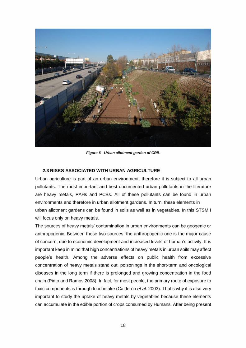
Figure 6 - Urban allotment garden of CRIL ................................................................. 18
Figure 7 - Illustration of the phenomenon of fluorescence ........................................... 20
Figure 8 – Sieving process.......................................................................................... 22
Figure 9 - fine sand fraction (< 2 mm) and the coarse fraction (> 2 mm) ..................... 23
Figure 10 - Percentage of fine sand and coarse fraction for each UAG ....................... 24
Figure 11 - Concentration of some elements in soil samples ...................................... 26
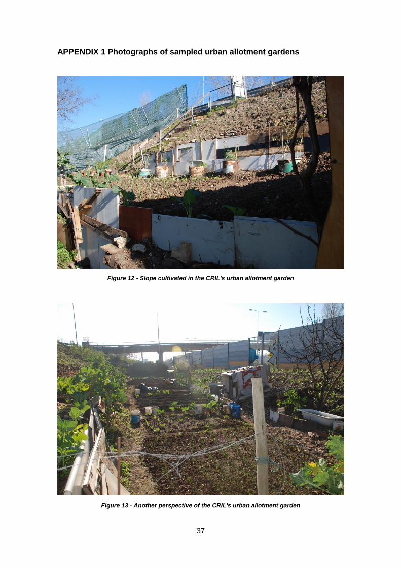
Figure 12 - Slope cultivated in the CRIL's urban allotment garden .............................. 37
Figure 13 - Another perspective of the CRIL's urban allotment garden ....................... 37
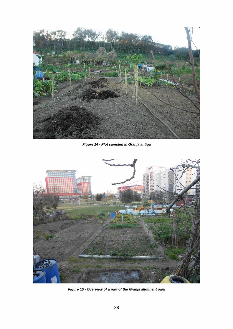
Figure 14 - Plot sampled in Granja antiga ................................................................... 38
Figure 15 - Overview of a part of the Granja allotment park ........................................ 38
Figure 16 - Plot sampled in Chelas ............................................................................. 39
Figure 17 - Greenhouses in the CHPL allotment garden ............................................. 39
Figure 18 – Equipment used in soil analysis ............................................................... 40
Table 1 - Legislated limit values for the analysed elements......................................... 27

6
1. INTRODUCTION
Most of the world population lives in cities, more specifically more than half of the world
population, and the United Nations expect that two-thirds of the planet Earth will live in
cities by 2050 (UN (United Nations) 2001). So, it’s essential that cities become more and
more sustainable. The sustainability concept isn’t new, it appeared applied to cities in
1992 at the United Nations Conference on Environment and Development (Eco-92), in
Rio de Janeiro, with a document called Agenda 21 (Howorth 2011) where the sustainable
urban development concept was defined and further on reaffirmed in 2002 at the World
Summit on Sustainable Development, in Johannesburg (Robert, Parris, and Leiserowitz
2005). Sustainable development is:
“…the development that meets the needs of the present without compromising the ability
of future generations to meet their own needs” (Brundtland 1987)
Since 1992 that the sustainability concept has become more popular and, at this
moment, it’s a key factor in many situations. This concept can be applied to cities. A
sustainable city has to incorporate the environmental dimension in its development,
protecting the environment. In addition, two more dimensions exist: the social justice and
the economic development (Buckingham-Hatfield and Percy 1999). The governmental
authorities have to take into account these three dimensions for a good sustainable
development. Therefore, an essential factor to obtain a sustainable city is to maintain or,
if possible, to increase the green areas in cities. These areas, covered in green urban
structure, join a wide number of ecologic functions beneficial for a lot of organisms in
urban environment. Furthermore, the green areas are recreational and leisure spaces
and a way to frame the urban structure. An example are the spaces where people grow
food in the city. These space are known as urban allotment gardens. In cities all over the
world the number of these gardens has increased, as well as the demand for them. In
times of crisis the demand for these spaces tend to increase (Dubbeling, Zeeuw, and
Veenhuizen 2010), given that growing its own food allows someone, who is going
through a bad financial time, to save money at the market. According to Pinto (2007) the
urban allotment gardens are an important environmental liberating, a supplement of
family income and an important source of proteins and vitamins for humans, allowing a
better use of the available resources in the interstitial spaces of urban ecosystems.
But not all points are positive: these agricultural spaces are inserted in urban areas so
they are exposed to a lot of pollution sources: traffic emission (vehicle exhaust particles,

7
tire wear particles, weathered street surface particles, brake lining wear particles),
industrial emission (power plants, coal combustion, metallurgical industry, chemical
plant), domestic emission, weathering of building and pavement surface and
atmospheric deposited (Wei and Yang 2010). These pollution sources are also a heavy
metals source, which is toxic for plants, animals and human beings above certain
quantities. Many researchers have showed urban soils contaminated with heavy metals
(Kapungwe 2013, Wei and Yang 2010, Kabala et al. 2009, Singh and Kumar 2006), so
it’s important to evaluate the heavy metals concentration in soils/plants of urban
allotment gardens. The soil is the support for plants, and some plants have the capability
of accumulating the soil metals. The individual that consumes contaminated vegetables
can have serious health problems, so the soil analysis is not only a study of its agricultural
capacity but also an indirect study to food safety of the products grown in them. The
analysis can be performed by various methods: instrumental neutron activation analysis
(INAA), X-ray based techniques, laser-induced breakdown spectroscopy (LIBS), laser
ablation inductively coupled plasma mass spectrometry (LA-ICP-MS), total digestion,
pseudototal digestion, single and sequential extraction, flame atomic absorption
spectrometry (FAAS) and inductively-coupled plasma atomic emission spectrometry or
mass spectrometry (ICP-AES, ICP-MS) (Alloway 2013).
In this Short Term Scientific Mission (STSM) the soils of six urban allotment gardens of
the city of Lisbon were analysed by portable X-ray fluorescence spectrometry (PXRF) at
Laboratory of Water and Environment (GERS department) of IFSTTAR, Nantes. The
PXRF it’s a non-destructive, fast and multi-element analyser methodology (Hou, He, and
Jones 2004). The portable apparatus are more accessible and the researcher have the
results faster than chemical methods, their limits of detection (LOD) are enough for the
environmental monitoring for most of soil’s elements, although the LOD of PXRF are
worse than conventional XRF laboratory equipment and Inductively Coupled Plasma
(ICP) technics (Shand and Wendler 2014).

8
2. URBAN AGRICULTURE
“Urban agriculture can be defined as the growing of plants and the raising of animals for
food and others uses within and around cities and towns, and related activities such as
the production and delivery of inputs, processing and marketing of products”
(Veenhuizen and Danso 2007)
Urban agriculture is not a new concept, it has existed since medieval times (Howorth
2011). Food production is linked to the city’s history from its origins. Before the industrial
revolution there was not an efficient transport system neither sophisticated techniques
to preserve food, therefore the population has to grow their own food near their home
(Southall 1998). With the beginning of 20th century urbanization, through the
constructions of highways, residential areas, railways and others infrastructures
necessary for the growth of cities, the urban agriculture spaces have slowly disappeared.
Only at the end of the 20th century the “Urban Agriculture” concept gained importance
through political and government agencies, they recognized that agricultural practice in
urban areas could have socio-economics benefits for the population (Howorth 2011). But
it was not only the politicians who gave importance to urban agriculture, also
researchers, urbanists and landscape architects have been giving a great importance to
this activity, making an activity that was neglected into an activity with a great potential
to create a form of sustainable livelihood. Thus, the urban agriculture is not only linked
to research related to the natural sciences (agronomy, pollution and water and soil
quality) but also to issues of social and economic nature (land transaction, rural flight
and social integration), to urban planning and to issues linked to architecture. A factor
that contributed to this change was 1960s’ new environmental ethics, with an alternative
lifestyle and a sense of self-sufficiency based on renewable energy (Matos and Batista
2013).
It is estimated that about 800 million people all over the world are, in some way, linked
to urban agriculture, both in developed countries and in developing countries, producing
approximately 15 % of food worldwide (predominantly fruit, vegetables, dairy and small
livestock) (FAO 2014). The scale of urban agriculture in the world is well above the
perception people have of this activity. For example, in Kenya and in Tanzania two in
three urban families are connected to agriculture, in Taiwan more than half of all urban
families are members of agricultural associations. The major Chinese cities produce
about 90 % of their needs in vegetables through urban agriculture, Japan, Netherlands
and Chile are examples of other countries where urban agriculture is well present in cities
(Smit and Nasr 1992).

9
In contrast to rural agriculture, urban agriculture is fully integrated in the urban system
through the use and reuse of urban natural resources (Mougeot 2000). In addition to
urban agriculture there is also a type of agriculture which is found on the border between
urban and countryside or suburban areas with low population density, this is the peri-
urban agriculture (Matos and Batista 2013). According to Mougeot (2005), the most
important characteristic that distinguishes urban agriculture of another type of agriculture
isn’t so much its location, but the fact that it constitutes a part of the urban economy and
of the ecological and social system. So the urban agriculture uses urban resources (land,
work, organic waste and water), produces for citizens, it is strongly influenced by urban
conditions (policies, land competition, markets and urban prices) and, finally causes
impact in urban system (effects on food security, poverty, ecology and health). The urban
agriculture can be present in different areas of cities in different forms, such as: urban
allotment gardens, urban landscaping with fruit trees, farms, plantation of medicinal
and/or ornamentals plants, grow vegetables along the roads, occupation of empty urban
lots and grow food at home in, for example, balconies, rooftops and courtyards (Pinto
2007). Most urban agriculture practitioners are involved is this activity as a livelihood
(Freeman 1993), using urban agriculture to get fresh food. These families can direct their
income to buy other essential products for Human diet. But the urban agriculture
objectives have been changing and the focus is not only alimentation. The urban
agriculture has been stimulated by urban sustainability, by the increase of food prices,
by the impoverishment of some social groups and by an increased awareness of
consumers about the origin of their food (Draper and Freedman 2010; Guitart, Pickering,
and Byrne 2012). This activity is often characterized by: being close to markets, present
high competitiveness for land, be located in a limited space, use organic residues namely
solid organic residues and waste waters, present a low degree of organization, its
products being mainly perishable and present a high degree of specialization (Matos and
Batista 2013).
The main environmental problems in urban areas are the poor air quality, the heat island
effect, floods, low ecological biodiversity, a stream of waste increasing and excessive
carbon emissions (Knizhnik 2012). Many of these problems can be solved through the
fomentation of urban agriculture, according to Cook, Lee, and Perez-Vazquez (2005) the
benefits of urban agriculture based on the following areas:
Social (leisure, fomenting local groups, therapy for individuals with special needs,
rehabilitation of youngsters);
Environmental (renewal of abandoned urban spaces, diversification of the usage
of urban land, increase of biodiversity, preservation of the water, soil and air
cycle, reduction of the carbon footprint);

10
Human (promotion of sociability through the encouragement of personal qualities
such as altruism, the improvement of the quality of life through social interaction,
health benefits through physical exercise, better food quality and bigger
diversity);
Economical (stimulus of the local economies, creation of employment and wealth,
directly or indirectly);
Emotional (due to the pause that it can provide to the monotonous and gray
everyday of the citizens, allowing them to realize the real dimension of time).
In literature there are many authors who share the same opinion about the urban
agriculture benefits (Vásquez-Moreno and Córdova 2013; Pearson, Pearson, and
Pearson 2010; Twiss et al. 2003; Putegnat 2001; Brown and Jameton 2000; Deelstra
and Girardet 2000).
In short, the benefits more frequently reported concerning urban agriculture, in the
literature reviewed are:
Reduces food transport distance, thus saving energy and reducing food
prices;
Reduces the heat island effect;
Contributes for the conservation of green spaces and urban soils;
Provides habitats for several species and contributes for local genetic
diversity;
Improves the physical and mental health of citizens;
Works as a strategy for halting the urban sprawl;
Improves the food security of cites.
Urban agriculture also has disadvantages, one of the biggest being restrictions the lack
of space in cities (Deelstra and Girardet 2000), and another well documented problem is
the contamination of soils and vegetables with some pollutants. The urban pollution has
being the potential to reduce the yield and the nutritional quality of vegetables (Jäger et
al. 1992).
2.1 URBAN SOILS
The soil formation is the result of complex biogeochemical processes involving numerous
abiotic and biotic factors, acting together. The soil is the interface with the atmosphere,
lithosphere, hydrosphere and biosphere (Schwartz et al. 2013), so it is a media with huge
importance in our world. For the soil formation the degradation and weathering of parent

11
rock is necessary, generating, through dissolution, oxidation and hydration, a wide range
of minerals which form the soil skeleton. The proportion of these soil minerals defines
the soil type (Schwartz et al. 2013). Unlike the original parent rock, the soil is a full of life
environment, dynamic, very reactive and constantly evolving (Lavelle and Spain 2005).
The soil has many functions, for example: it is the physical and nutritional support for
plant growth, it is the habitat for soil organisms including organic matter decomposers, it
acts as a filter for water and also serves to support human diets ((Gobat, Aragno, and
Matthey 2010; Vannier 1979).
The soil is comprised by a solid phase and also a gaseous (soil pores) and liquid phase.
The solid phase is known as soil matrix and contains the mineral and organic materials.
The gaseous phase is termed soil atmosphere and the liquid phase represents the soil
water with dissolved substances, it is also known as soil solution (Costa 1975). Thus, we
can conclude that soil has four essential functions (Varennes 2003):
1. Supports plant growth, providing the environment for the development of the
roots and providing water and nutrients for plants.
2. Recycles waste and dead tissues of animals and organisms, becoming the
elements of these materials available again.
3. Provides ecological niches where millions of organisms live, from small mammals
to fungi and bacteria.
4. Controls the water movement and its quality in watersheds.
Urban areas are an ecosystem dominated by human beings, giving us the opportunity to
study the anthropogenic influence on soil. The urban soils are very altered due to the
anthropogenic activities, such as: compression by heavy equipment, topsoil removal,
atmospheric deposition of toxic compounds, heavy metal contamination, intensive
application of fertilizers and chemical pesticides and contamination due to transports and
industry (Pouyat et al. 2010; Lohse et al. 2008). According to Park et al. (2010) the
anthropogenic disturbance on urban soils can be seen in two different ways:
The first one is related with initial urban development. Typically, these
perturbations are drastic, involving modifications on soil profile, removing or
adding soil, compaction and introduction of vegetation.
The second one is related with less drastic perturbations, but still harmful. These
forms of disturbance include the changes from chemical inputs, such as
atmospheric deposition, fertilizers and chemical pesticides applications and
precipitation runoff that can be contaminated due to urban activities.
The green urban structure of cities includes cemeteries, green along traffic, all parks,
gardens and urban allotment gardens. The soils of urban allotment gardens are very
similar morphologically and functionally to agricultural soils. However they differ from the

12
last one in management, composition and use from the last ones. In fact, the uses of
urban soils vary quite often to adapt the spaces to the needs (Putegnat 2001). As the
cities are constantly changing, the urban soils suffer with these changes.
One important thing to do in urban soils is to evaluate their quality. According to Doran
and Parkin (1994), the soil quality is defined as the capacity of a soil to function within
ecosystem boundaries to sustain biological productivity, maintain environmental quality
and promote plant and animal health. The soil contamination is a real problem in many
cities (Heinegg et al. 2002), they can be contaminated with, for example, heavy metals
(Kapungwe 2013), polycyclic aromatic hydrocarbons (PAHs) (Tang et al. 2005) and
polychlorinated biphenyl (PCB) (Wilcke et al. 1999). There are several problems
associated with soil contamination, plants can uptake these contaminants that will
generate health problems if Humans consume them. Another problem is the accidental
ingestion of contaminated soil particles. The accidental ingestion can be derived from
badly washed hands, inhalation of dusts and eating unwashed or badly washed food
(Abrahams 2002). I have been referring contamination of urban soils, but it is important
to distinguish between “contamination” and “pollution”. A contamination case means that
one or more substances have accumulated. In normal cases, these substances wouldn’t
be in soil or at least would be at a lower level. On other hand, a pollution case means
that the presence of these substances can affect the living organisms (Varennes 2003).
As I have seen, the urban allotment gardens constitute one of the urban soils uses. In
the next subchapter I will address the thematic of urban allotment gardens, specifying
for the Lisbon case.
2.2 URBAN ALLOTMENT GARDENS – LISBON CASE
The implementation of urban allotment gardens in Portugal is a slightly recent
phenomena unlike most of Northern European countries (Rodrigues et al. 2014). It was
in Lisbon were the first forms of urban agriculture emerged, responding to social changes
that were related to migrations and immigration movements towards the city during
1960’s and 1970’s (Matos and Batista 2013) . During this time, plots of vacant land were
occupied, and improvised, clandestine and illegal allotments emerged. In the past
decade, the number of urban allotment gardens in Portugal have increased due to the
effort of municipalities and stakeholders to create areas for this activity and legalize and
provide better conditions to the existing ones (Rodrigues et al. 2014). The urban
allotment gardens are responding to new needs for leisure and occupation, reconnecting
people to land, countryside and nature. For these reasons, but also because of budget

13
constraints, urban allotment gardens are being offered as an alternative way of open
space with reduced maintenance, which provide sustenance and opportunities for
recreation, fostering social cohesion and well-being (Dunnett and Qasim 2000). The
urban allotment gardens also have educational and pedagogical benefits, where the
knowledge can be shared inter-generationally and citizens can learn practices of growing
food (Rodrigues et al. 2014)
Urban allotment gardens, as has been seen, are one of the main ways to practice
agriculture within city. An allotment is characterized as a small agricultural plot where are
grown food, such as vegetables, greenery or fruit trees, but it’s also possible cultivate
non-food products, such as ornamental or medicinal plants. If these products (food or
non-food) are produced within urban system, then this activity is called urban allotment
garden (Pinto 2007). The soils of urban gardens are thus specific agricultural soils,
localized in urbanized environments and subjected to an intensive agriculture. The urban
allotment gardens are placed in areas that have a high biological value because of their
moisture characteristics and deeper soil. Plus, the frequent mobilizations and
incorporations of organic matter increase the level of microbial life soil and contributes
significantly for the maintenance of food webs.
In Portugal a national policy for urban allotment gardens has not yet been developed.
This activity is often planned and managed by public or private entities at a local level.
Some cities have created programmes to encourage their implementation and in some
cases they are integrated in the green infrastructure, or allocated under the land use
category of “production and recreational zones” (Rodrigues et al. 2014). This is the case
of the municipality of Lisbon, where the urban allotment gardens are found in “production
and recreational” zones of Municipal Master Plan (MMP) of Lisbon. The categories of
allotments covered by the MMP are social allotment gardens, recreational allotment
gardens and pedagogical allotment gardens. Lisbon City Council with the introduction of
urban agriculture intends to:
Contribute to greater environmental sustainability of the city at various levels,
namely maintaining ecosystems, contributing to an improvement of microclimate,
improving soil quality by organic correction and appropriate cultural mobilizations
and improving water systems by increasing soil permeability;
Contribute to the supply of fresh food in urban centres;
Contribute to an improvement in public health;
Value landscape and environmentally urban areas by spatial organization of
indefinite use areas;
Value culturally by general awareness of the population to ancient production
systems, approaching city population to rural areas;

14
Sensitize all citizens from different social strata for the importance of fresh food
and for the nutritional and economic advantages of organic farming.
I mentioned that Lisbon’s urban allotment gardens covered by MMP are social,
recreational and pedagogical allotment gardens, but what are the main objectives of
each one?
Social allotment gardens
The social gardens are used by families or individuals. Their main objectives are to
satisfy food needs of individuals/families with few monetary resources. These allotments
are intended, therefore, for food production for self-consumption and sometimes, if there
is surpluses, to sell the products in local markets with the objective of improve
farmer/family incomes.
Recreational allotment gardens
The recreational allotment gardens are also used by families or individuals, its main
objectives are the leisure and recreation of users. Users of these type of allotment
gardens see in this type of activity an opportunity to improve their quality of life, since
they have the chance to escape to city stress and day-to-day work with an approach to
rural world.
Under this classification, it also exists community allotment gardens, which are for
collective use of residents groups and have as purpose the leisure, recreation and
environmental education of communities. They also serve to increase contact among
people from the same neighbourhood, by exchanging experiences, thereby increasing
social cohesion.
Pedagogical allotment gardens
The aim of these allotment gardens is the environmental education through natural
sciences, work and socialization in the garden. They are intended mostly to younger
people in order to have, from an early age, a strong environmental awareness of the
benefits that agriculture can have. Users can also acquire knowledge about crop cycle,
collaborating in agricultural activities necessary for the proper development of allotment
gardens. Usually these gardens are inserted in so-called “pedagogical farms” where
besides horticultural aspects the people may have contact with many rural traditions.
In the beginning of this subchapter was mentioned that the vacant land plots were
occupied during the 1960’s and 1970’s. In fact, Lisbon’s unregulated allotment gardens

15
reached 300 ha between 1970 and 1987, between 1987 and 1995 this area reduced to
approximately 100 ha and stabilized (Cabannes and Raposo 2013). Since 2007, there
is a municipal program that is converting several areas in allotment parks. These
allotment parks, apart from spaces dedicated to agriculture, also have lawned areas,
playgrounds, kiosks, fitness equipment and cycle paths. The first two parks were
inaugurated in 2011 – “Quinta da Granja” and “Jardins de Campolide” – and in 2012 was
opened another one – “Parque Hortícola de Telheiras Nascente”. In 2013 Lisbon City
Council created five more parks – “Quinta de Nossa Senhora da Paz”, “Parque
Bensaúde”, “Parque dos Olivais”, “Parque Vale de Chelas” and in the surrounding of
“Cerca da Graça”. Last year the “Parque Hortícola da Boavista” and “Hortas do
Casalinho da Ajuda” were inaugurated. In total, in 2014, the city has 10 allotment parks,
serving over 400 families. The Lisbon City Council will open more parks, two of them will
be in the areas of National Laboratory of Civil Engineering (LNEC) and Psychiatric
Hospital of Lisbon (CHPL) (“Parques Hortícolas Municipais” 2015). Currently there are
already allotment gardens in these areas, but they are not regulated by Lisbon City
Council.
For my STSM I sampled the soils in some of these gardens. As it will be seen later, the
allotment parks used were: “Quinta da Granja”, “Parque Vale de Chelas” and allotment
gardens of LNEC and CHPL. In addition to these allotment gardens, the soil of one non-
regulated allotment garden in the edge of a motorway was also sampled. Below are
displayed the photographs of sampled urban allotment gardens. For more photographs
see the appendix 1.
Figure 1 - Urban allotment garden of Granja antiga

16
Figure 2 - Urban allotment garden of Granja nova
Figure 3 - Urban allotment garden of Vale de Chelas

17
Figure 4 - Urban allotment garden of LNEC
Figure 5 - Urban allotment garden of CHPL
18
Figure 6 - Urban allotment garden of CRIL
2.3 RISKS ASSOCIATED WITH URBAN AGRICULTURE
Urban agriculture is part of an urban environment, therefore it is subject to all urban
pollutants. The most important and best documented urban pollutants in the literature
are heavy metals, PAHs and PCBs. All of these pollutants can be found in urban
environments and therefore in urban allotment gardens. In turn, these elements in
urban allotment gardens can be found in soils as well as in vegetables. In this STSM I
will focus only on heavy metals.
The sources of heavy metals’ contamination in urban environments can be geogenic or
anthropogenic. Between these two sources, the anthropogenic one is the major cause
of concern, due to economic development and increased levels of human’s activity. It is
important keep in mind that high concentrations of heavy metals in urban soils may affect
people’s health. Among the adverse effects on public health from excessive
concentration of heavy metals stand out: poisonings in the short-term and oncological
diseases in the long term if there is prolonged and growing concentration in the food
chain (Pinto and Ramos 2008). In fact, for most people, the primary route of exposure to
toxic components is through food intake (Calderón et al. 2003). That’s why it is also very
important to study the uptake of heavy metals by vegetables because these elements
can accumulate in the edible portion of crops consumed by Humans. After being present
19
in Human body heavy metals are easily accumulated due to their non-biodegradable
nature and long half-life times for elimination (Guo et al. 2012).
In subchapter “2.1 Urban Soils” it was reported that one of the several problems
associated with soil contamination is the accidental ingestion of contaminated soil
particles. This exposure route is most significant for children due to the time they spend
outdoors, getting to mouth objects or their hands that may have been in contact with
contaminated soil. Abrahams (2002) analysed data from several studies about the
amount of ingested soil by children in various age groups and concluded: the children
aged 1-4 years ingest 9-96 mg d-1, children aged 6-12 years ingest only 25 % of the
amount of soil consumed by the previous age group and children over 12 years don’t
ingest more than 10 % of the amount ingested by children aged 1-6 years. Adults only
ingest an average of 10 mg d-1.
3. X-RAY FLUORESCENCE SPECTROMETRY
It was in 1895 that Wilhelm Röntgen discovered X-rays. X-rays are a form of
electromagnetic radiation, as are radio waves, infrared radiation, visible light, ultraviolet
radiation and microwaves (Lucas 2015).
X-ray fluorescence (XRF) spectrometry is a widely-used technique for routine
determination of the major elements as well as trace elements. The use of XRF
spectrometers for elemental analysis became widespread in the 1950’s early 1960’s.
The researchers who had led to this technique is now possible were, firstly Barkla who
observed the X-ray emission spectra and then Moseley, who established a relationship
between the frequency (𝜈) and the atomic number of each element (Ζ) by a law:
𝜈 = 𝐾(Ζ − 𝜎)2
where 𝐾 and 𝜎 are both constants that vary with the spectral series. It was this discover
that made possible the use of this technique (Jenkins, Gould, and Gedcke 1995).
The analysis per XRF is a method based on measuring the intensity of the characteristic
X-rays emitted by elements in sample, when excited by electromagnetic waves. The XRF
spectrometry is a non-destructive and quick method that analyse simultaneously several
elements, this method has been being developed to be included in portable devices
(Hou, He, and Jones 2004). In my STSM the analysis of the soil samples were performed
using a portable XRF spectrometer (PXRF). During the last 10 years the PXRF devices
have been developing quickly (Weindorf, Bakr, and Zhu 2014), gaining popularity among
the scientific community through publishing several papers about various themes: pH
determination (Sharma et al. 2014), soil texture (Zhu, Weindorf, and Zhang 2011),

20
identification of soil horizons (Weindorf et al. 2011), identifying contaminants in the soil
(Hürkamp, Raab, and Völkel 2009), analysis of plant nutrients (McLaren, Guppy, and
Tighe 2011) and it was also used in agronomy applications (Paltridge et al. 2012).
3.1 PRINCIPLES OF X-RAY FLUORESCENCE
An atom is formed by a nucleus around which the electrons gravitate. These electrons
are located in different orbits – K, L, M and N – that have well-defined energy levels.
When samples are excited by a primary beam of X-rays, interaction of X-rays photons
with atoms causes the ionisation of inner shell orbital electrons. As the inner shell
electron is ejected the atom becomes unstable, so one outer shell electron occupies the
empty place. This transition releases energy in the form of X-ray photons originating the
fluorescence phenomenon which are specific of each element (Sharma et al. 2015), the
energy involved in this transition can be measured and corresponds to the energy
difference between the two orbitals. The devices measure the intensity of the
characteristic fluorescence radiation of each element.
For all XRF spectrometers the analytical scheme can be divided into four phases
(Jenkins, Gould, and Gedcke 1995):
1. Excitation of sample’s atoms by bombardment with high-energy photons;
2. Selection of a characteristic emission line of an element by wavelength dispersive
spectrometer or an energy dispersive spectrometer;
3. Detection and integration of the characteristic photons to give a measure of the
intensity of the characteristic line emission;
4. Conversion of the intensity of the characteristic line emission to a value of
element concentration using an appropriate calibration procedure.
Figure 7 - Illustration of the phenomenon of fluorescence (source: Thermo Scientific equipment catalog)

21
4. METHODOLOGY
4.1 SOIL SAMPLING
The soil sampling was made on June 17th in six urban allotment gardens of Lisbon:
UAG regulated by city council:
o “Quinta da Granja” that was divided into two zones – old part (“Granja
antiga”) and new part (“Granja nova”);
o “Parque Vale de Chelas”;
Private UAG:
o UAG of National Laboratory of Civil Engineering (LNEC);
o UAG of Psychiatric Hospital of Lisbon also known as “Júlio de Matos
Hospital” (CHPL);
Non-regulated UAG:
o UAG of CRIL. CRIL means internal ring road of Lisbon and is a motorway
with an average car traffic of 75 000 vehicles per day (Silva, Ramos, and
Lourenço 2010).
Samples were taken at one depth (0-5 cm) to study the anthropogenic inputs because
the topsoil layer has, almost entirely, the contamination that came through anthropogenic
inputs, while the deeper soil layers contain mostly concentration which had natural origin
(Facchinelli, Sacchi, and Mallen 2001) or was leached by the infiltration of precipitation.
In each urban allotment garden 3 plots were chosen, and in each one of these plots the
soil was collected from 3 different points. The soils were collected with a plastic spade
due to the possibility of residual contamination through metal materials. In total 18 bags
were collected, and transported, by plane, to IFSTTAR (The French Institute of Science
and Technology for Transport, Development and Networks), in Nantes, France. Before
the transport, the soils were dried at 40 ºC at LNEC laboratory during two days.
From now on all the work described was performed in IFSTTAR.
4.2 SOIL ANALYSIS
First of all, a plan of what could be done with the soil samples was done, by Béatrice
Bechet and me. The following tasks were decided to be performed:
1. Sieve the soil samples into two fractions – < 2 mm and > 2 mm;
2. Milling the < 2 mm fraction for analysis in the PXRF spectrometer;
3. Analyse the soil samples with PXRF spectrometer;

22
4. Sieve the < 2 mm fraction into > 250 𝜇𝑚, [250 – 63] 𝜇𝑚, < 63 𝜇𝑚;
5. Analyse the previous fractions with PXRF spectrometer;
6. Select a sample of each UAG to analyse by ICP techniques.
1. Sieve the soil samples into two fractions - < 2 mm and > 2 mm
Before sieving the soils, they were dried again, due to temperature differences
experienced in the plane’s baggage compartment. This time they were air dried during
two days. The soil samples were sieved with a 2 mm mesh (Figure 8), obtaining two
fractions - the fine sand fraction (< 2 mm) and the coarse fraction (> 2 mm) (Figure 9).
Each fraction was put into separate bags, properly identified with laboratory reference,
Portuguese reference and fraction. Each bag was weighed and its weight registered. The
sieving process was carried out using an hotte and I was using rubber gloves to do the
sieving to prevent any contamination. The equipment was washed between each sieving
first with tap water and then with deionized water.
2. Milling the < 2 mm fraction
For the PXRF analysis the < 2 mm fractions have to present a fine texture in order to
facilitate the penetration of X-rays. So the milling process was carried out using the
following equipment: Pulvérisette 6, SPRITCH. For each sample 50 g of soil was put into
a bowl with 6 balls for 3 minutes at 400 rpm, the bowl was put inside the equipment. The
milled soil was transferred to plastic vials. Between each milling the bowl was cleaned
with sand and 10 mL of water with 6 balls inside during 15 seconds at 400 rpm.
Figure 8 – Sieving process. On the left the sample before sieving, on the right the same sample after sieving

23
3. Analyse the soil samples with PXRF spectrometer
The samples that were analysed were those which were put in vials, so the milled < 2
mm fraction. The equipment used was the Thermo Scientific Niton Xl3t goldd. All the
samples were analysed using two modes – mineral and soil mode – these modes are
characteristic of the equipment. For both modes the samples were analysed during 120
seconds, performing three repetitions.
4. Sieve the < 2 mm fraction into > 250 μm, [250 – 63] μm, < 63 μm
This task was done to better understand in which fraction contamination is allocated,
analysing then these fractions by PXRF spectrometry. The equipment used to shake the
sieves was the Analysette 3, FRITSCH. It was made a dry sieving to obtain the > 250
𝜇𝑚, [250 – 63] 𝜇𝑚 and < 63 𝜇𝑚 fractions, each sieving lasted 5 minutes and the shake
amplitude was 2,0 mm. The division of fractions and the washing of sieves are the same
as done in point 1.
Figure 9 - fine sand fraction (< 2 mm) on the left and the coarse fraction (> 2 mm) on the right

24
All the photographs of the used equipment are in appendix 2 and the limits of detection
of the PXRF spectrometer in appendix 3.
In my stay at IFSTTAR were these tasks that were performed, the other tasks (points 5
and 6) will be performed by the laboratory technique and then the results will be sent to
me. So I can’t present all results in this short report. The remaining results will be
presented in the longer scientific report.
5. RESULTS AND DISCUSSION
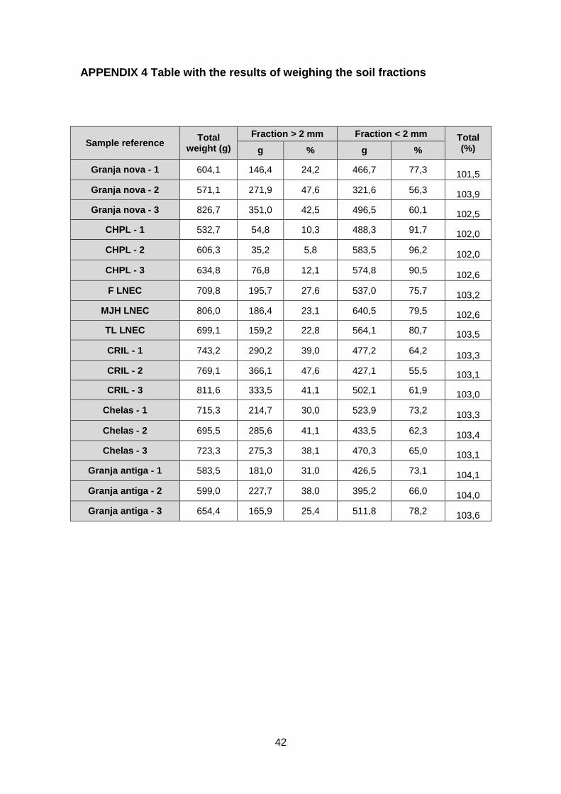
After sieving the soil samples between fine sand fraction and coarse fraction, the results
of weighing the fractions are presented in appendix 4 as well as the percentages
corresponding to each fraction. To facilitate comparison between different urban
allotment gardens a graph was made gathering the three plots of each UAG, so the chart
values are the mean values.
Figure 10 - Percentage of fine sand and coarse fraction for each urban allotment garden
Through the analysis of the figure 10 we have concluded that the samples with coarser
elements are: CRIL and Granja nova. On the other hand the sample that presents a
higher percentage of fine sand fraction is: CHPL. The soils of CRIL allotment garden
0,0
10,0
20,0
30,0
40,0
50,0
60,0
70,0
80,0
90,0
100,0
Fraction > 2 mm Fraction < 2 mm
(%)
Granja nova CHPL LNEC CRIL Chelas Granja antiga

25
present a lot of construction materials and solid objects from the surrounding roads (see
figure 6 to better understand the surroundings), including pieces of mosaics and bricks.
After the sieving the soils were analysed by PXRF spectrometer. To find out if the values
are within legal limits I have used two documents, one of them is part of the Portuguese
law and the other is part of Canadian law. In Portugal the only governmental document
that has heavy metals limits to soils is the Ordinance n.º 176/96 (2nd series) of October
3rd, Ministries of agriculture, rural development and fisheries and environment. This
ordinance regulates the concentration of heavy metals in the soils that will receive
sludge, the amount of heavy metals in sludge for agricultural utilization as fertilizer as
well as the maximum amount of heavy metals that can be introduced annually in the soil.
The Portuguese legislation only provides values for cadmium, copper, nickel, lead, zinc,
mercury and chromium to the following pH ranges: pH ≤ 5.5; 5.5 < pH ≤ 7.0; pH > 7.0.
For elements not covered by this ordinance the Portuguese government recommends
the use of Canadian legislation, more specifically the Soil, Ground Water and Sediment
Standards for use under Part XV.1 of the Environmental Protection Act (2011). This
documents has an exhaustive list of elements and their limit values.
The limit values for the analysed elements in my STSM are listed in table 1, note that for
some elements neither document has limit values.
After the analysis of the soils by PXRF spectrometer, a table was constructed with all
concentration values for each element. The table in appendix 5 is the result of data
processing, it was made by the mean of three repetitions. With this data the following
boxplot was constructed, to facilitate the visualization of dispersion of elements
concentrations. The box plot only shows the elements for which there are limit values,
where the red line represents those thresholds, and also only the elements that have
enough concentration values to represent a good box plot (i.e. the elements with most
of values below the limit of detection are omitted).

26
Figure 11 - Concentrations of some elements in soil samples
Looking to figure 11 and appendix 5, we can conclude that some concentrations are
above the thresholds. I will group the discussion of the concentration values by element,
but I will only consider those with threshold:
Arsenic:
For this element the maximum permitted concentration is 11 mg kg-1, analysing the
appendix 5 it can be seen that all samples are below the limit of detection (LOD) except
one – “MJH LNEC” – which has the concentration of 18.13 mg kg-1.
Barium:
Barium was found in almost all samples, but always below the threshold. Only the UAG
of CRIL shows evidence of contamination with concentrations above 390 mg kg-1, this
can be seen at figure 11. At the others sites the mean concentration is, approximately,
150 mg kg-1.

27
Table 1 - Legislated limit values for the analysed elements
ELEMENT Ordinance n.º 176/96
Soil, Ground Water and Sediment Standards for use under Part
XV.1 of the Environmental Protection Act
(mg kg-1) (mg kg-1)
Aluminium (Al) - -
Arsenic (As) - 11
Barium (Ba) - 390
Bismuth (Bi) - -
Calcium (Ca) - -
Cadmium (Cd) 4 1
Cobalt (Co) - 22
Chromium (Cr) 300 160
Copper (Cu) 200 180
Iron (Fe) - -
Mercury (Hg) 2 1,8
Potassium (K) - -
Magnesium (Mg) - -
Manganese (Mn) - -
Molybdenum (Mo) - 6,9
Nickel (Ni) 110 130
Phosphorus (P) - -
Lead (Pb) 450 45
Antimony (Sb) - 7,5
Selenium (Se) - 2,4
Silicon (Si) - -
Strontium (Sr) - -
Titanium (Ti) - -
Vanadium (V) - 86
Zinc (Zn) 450 340
Cadmium:
Cadmium is an element whose concentration is below the LOD for all samples, so this
element doesn’t need specific concern by local authorities.

28
Cobalt:
The threshold for this element is 22 mg kg-1. There are only two plots with concentrations
above the threshold all other are below the LOD. These plots are “Granja nova – 1” and
“CRIL – 1” with 90.97 and 210.44 mg kg-1, respectively.
Chromium:
This element was only measured in Granja nova and CRIL allotment gardens, for the
remaining sites the concentration is below the LOD. The maximum measured value was
105 mg kg-1 in “CRIL – 3” and the minimum was measured in “Granja nova – 3” with
35.44 mg kg-1.
Copper:
All measured values are clearly below the threshold, 200 mg kg-1. The highest values
are found in CRIL and Granja antiga, with mean values of 54.21 and 67.25 mg kg-1,
respectively. For all other urban allotment gardens the concentration of copper in soils is
very similar.
Mercury:
As well as cadmium, mercury also has all measurement below the LOD.
Molybdenum:
The concentration of this element doesn’t vary too much between plots, the range is
[2.76, 4.48] mg kg-1, being this values lower than the threshold. For Granja nova, CHPL
and Chelas all plots have values below the LOD.
Nickel:
Nickel concentration is lower than LOD in all urban allotment garden, except the CRIL’s
urban allotment garden. At this location the mean value between the three plots is 93.69
mg kg-1, which is a lower value that the threshold.
Lead:
Lead is one of the most analysed element in urban environments, sometimes with
concentrations higher than recommended. The threshold for lead is very different if we
use the Portuguese legislation (450 mg kg-1) or the Canadian legislation (45 mg kg-1). If
we use the Portuguese legislation, all concentration values are below the threshold. On
29
the other hand, if Canadian legislation was used there are some value above the
threshold: two plots in CHPL, one plot in LNEC and all plots in Granja antiga.
Surprisingly, CRIL’s allotment garden has lower values than Granja antiga. Granja antiga
is the furthest allotment garden of pollution sources.
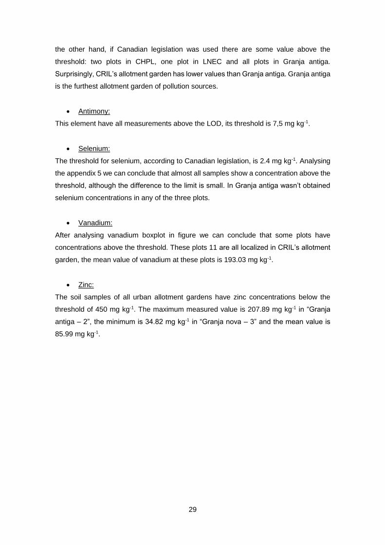
Antimony:
This element have all measurements above the LOD, its threshold is 7,5 mg kg-1.
Selenium:
The threshold for selenium, according to Canadian legislation, is 2.4 mg kg-1. Analysing
the appendix 5 we can conclude that almost all samples show a concentration above the
threshold, although the difference to the limit is small. In Granja antiga wasn’t obtained
selenium concentrations in any of the three plots.
Vanadium:
After analysing vanadium boxplot in figure we can conclude that some plots have
concentrations above the threshold. These plots 11 are all localized in CRIL’s allotment
garden, the mean value of vanadium at these plots is 193.03 mg kg-1.
Zinc:
The soil samples of all urban allotment gardens have zinc concentrations below the
threshold of 450 mg kg-1. The maximum measured value is 207.89 mg kg-1 in “Granja
antiga – 2”, the minimum is 34.82 mg kg-1 in “Granja nova – 3” and the mean value is
85.99 mg kg-1.

30
6. CONCLUSION
First of all, it’s important to say that the results will be analysed in depth in the longer
scientific report. In this short report I only analyse superficially the results. I tried to give
an idea of heavy metals and remaining elements distribution through urban allotment
gardens. So we can conclude that the urban allotment garden with more concentration
values above the elements threshold is CRIL, showing contamination with barium,
cobalt, selenium and vanadium. For the longer scientific report will be analysed the
geology of each allotment park, to better understand if the measured values have natural
or anthropogenic origin. In addition, will be also analysed the influence of each element
in human’s health.
This short term scientific mission in IFSTTAR was very helpful for me at personal level
as well as professional level. What has been learned will be very important for the
conclusion of my master’s thesis. I realized that it’s important to reflect about urban locals
where is acceptable the introduction of urban allotment gardens, urban planners have to
take into account several factors for the proper functioning of these parks. It is
recommended to perform an early environmental assessment of urban allotment
gardens, in order to identify possible problems of contamination and urban pollution.

31
7. REFERENCES
Abrahams, P.W. 2002. “Soils: Their Implications to Human Health.” Science of The Total Environment 291 (1-3): 1–32. doi:10.1016/S0048-9697(01)01102-0.
Alloway, B. J. 2013. Heavy Metals in Soils: Trace Metals and Metalloids in Soils and Their Bioavailability. 3rd editio. Springer Dordrecht Heidelberg New York London. doi:10.1007/978-94-007-4470-7.
Brown, K. H., and A. L. Jameton. 2000. “Public Health Implications of Urban Agriculture.” Journal of Public Health Policy 21 (1): 20–39.
Brundtland, G. H. 1987. “Our Common Future: The Report of the World Commission on Environment and Development,” 1–300.
Buckingham-Hatfield, S., and S. Percy. 1999. Constructing Local Environmental Agendas: People, Places, and Participation. Routledge.
Cabannes, Y., and I. Raposo. 2013. “Peri-Urban Agriculture, Social Inclusion of Migrant Population and Right to the City.” City: Analysis of Urban Trends, Culture, Theory, Policy, Action 17 (2): 235–50. doi:10.1080/13604813.2013.765652.
Calderón, J., D. Ortiz-Pérez, L. Yáñez, and F. Dı́az-Barriga. 2003. “Human Exposure to Metals. Pathways of Exposure, Biomarkers of Effect, and Host Factors.” Ecotoxicology and Environmental Safety 56 (1): 93–103. doi:10.1016/S0147-6513(03)00053-8.
Cook, H. F., H. C. Lee, and A. Perez-Vazquez. 2005. “Allotments, Plots and Crops in Britain.” In Continuous Productive Urban Landscapes, 206–16. Elsevier GmbH.
Costa, J. B. 1975. Caracterização E Constituição Do Solo. Lisboa: Fundação Calouste Gulbenkian.
Deelstra, T., and H. Girardet. 2000. “Urban Agriculture and Sustainable Cities.” Urban Agriculture and Sustainable Cities, 43–65. doi:10.1177/095624789200400214.
Doran, J. W., and T. B. Parkin. 1994. “Defining and Assessing Soil Quality.” In Defining Soil Quality for a Sustainable Environment, 3–21. Soil Science Society of America.
Draper, C., and D. Freedman. 2010. “Review and Analysis of the Benefits, Purposes, and Motivations Associated with Community Gardening in the United States.” Journal of Community Practice 18 (4): 458–92. doi:10.1080/10705422.2010.519682.
Dubbeling, M., H. de Zeeuw, and R. van Veenhuizen. 2010. Cities, Poverty and Food: Multi-Stakeholder Policy and Planning in Urban Agriculture.
Dunnett, N., and M. Qasim. 2000. “Percieved Benifits to Human Well-Being of Urban Gardens.” HortTechnology 10 (1): 40–45.
Facchinelli, A., E. Sacchi, and L. Mallen. 2001. “Multivariate Statistical and GIS-Based Approach to Identify Heavy Metal Sources in Soils.” Environmental Pollution 114 (3): 313–24. doi:10.1016/S0269-7491(00)00243-8.

32
FAO. 2014. Ciudades Más Verdes En América Latina Y El Caribe. Edited by G. Thomas. Rome.
Freeman, D. B. 1993. “Survival Strategy or Business Training Ground? The Significance of Urban Agriculture for the Advancement of Women in African Cities.” African Studies Review 36 (03): 1–22. http://dx.doi.org/10.2307/525171.
Gobat, J.-M, M. Aragno, and W. Matthey. 2010. Le Sol Vivant: Bases de Pédologie - Biologie Des Sols. 3rd editio. Presses Polytechniques et Universitaires Romandes.
Guitart, D., C. Pickering, and J. Byrne. 2012. “Past Results and Future Directions in Urban Community Gardens Research.” Urban Forestry and Urban Greening 11 (4). Elsevier GmbH.: 364–73. doi:10.1016/j.ufug.2012.06.007.
Guo, G., F. Wu, F. Xie, and R. Zhang. 2012. “Spatial Distribution and Pollution Assessment of Heavy Metals in Urban Soils from Southwest China.” Journal of Environmental Sciences 24 (3). The Research Centre for Eco-Environmental Sciences, Chinese Academy of Sciences: 410–18. doi:10.1016/S1001-0742(11)60762-6.
Heinegg, A., P. Maragos, M. Edmund, J. Rabinowicz, G. Straccini, and H. Waish. 2002. Soil Contamination and Urban Agriculture - A Practical Guide to Soil Contamination Issues for Individuals and Groups.
Hou, X., Y. He, and B. T. Jones. 2004. “Recent Advances in Portable X‐Ray Fluorescence Spectrometry.” Applied Spectroscopy Reviews 39 (1): 1–25. doi:10.1081/ASR-120028867.
Howorth, A. 2011. “As Hortas Da Área Metropolitana de Lisboa: Caracterização E Fertilidade Dos Solos.” Instituto Superior de Agronomia, Universidade Técnica de Lisboa. http://www.repository.utl.pt/handle/10400.5/4204.
Hürkamp, K., T. Raab, and J. Völkel. 2009. “Two and Three-Dimensional Quantification of Lead Contamination in Alluvial Soils of a Historic Mining Area Using Field Portable X-Ray Fluorescence (FPXRF) Analysis.” Geomorphology 110 (1-2): 28–36. doi:10.1016/j.geomorph.2008.12.021.
Jäger, H. J., M. Unsworth, L. De Temmerman, and P. Mathy. 1992. Effects of Air Pollution on Agricultural Crops. Brussels: Commissionof the European Communities.
Jenkins, R., R. W. Gould, and D. Gedcke. 1995. Quantitative X-Ray Spectrometry. 2nd editio. USA: Marcel Dekker, Inc.
Kabala, C., T. Chodak, L. Szerszen, A. Karczewska, K. Szopka, and U. Fratczak. 2009. “Factors Influencing the Concentration of Heavy Metals in Soils of Allotment Gardens in the City of Wroclaw, Poland.” Fresenius Environmental Bulletin 18 (7): 1118–24.
Kapungwe, E. M. 2013. “Heavy Metal Contaminated Water , Soils and Crops in Peri Urban Wastewater Irrigation Farming in Mufulira and Kafue Towns in Zambia.” Journal of Geography and Geology 5 (2): 55–72. doi:10.5539/jgg.v5n2p55.

33
Knizhnik, H. L. 2012. “The Environmental Benefits of Urban Agriculture on Unused, Impermeable and Semi-Permeable Spaces in Major Cities with a Focus on Philadelphia , PA.” University of Pennsylvania. http://repository.upenn.edu/mes_capstones/46.
Lavelle, P., and A. V. Spain. 2005. Soil Ecology. 2nd editio. Netherlands: Springer.
Lohse, K. A., D. Hope, R. Sponseller, J. O. Allen, and N. B. Grimm. 2008. “Atmospheric Deposition of Carbon and Nutrients across an Arid Metropolitan Area.” The Science of the Total Environment 402 (1): 95–105. doi:10.1016/j.scitotenv.2008.04.044.
Lucas, J. 2015. “What Are X-Rays?” http://www.livescience.com/32344-what-are-x-rays.html.
Matos, R. S., and D. S. Batista. 2013. “Urban Agriculture : The Allotment Gardens as Structures of Urban Sustainability.” Advances in Landscape Architecture, 457–512. http://dx.doi.org/10.5772/55892.
McLaren, T. I., C. N. Guppy, and M. K. Tighe. 2011. “A Rapid and Nondestructive Plant Nutrient Analysis Using Portable X-Ray Fluorescence.” Soil Science Society of America 76 (4): 1446–53.
Mougeot, L. J. A. 2000. “Urban Agriculture: Definitions, Presence, Potentials and Risks.” Growing Cities, Growing Foods: Urban Agriculture on the Policy Agenda, 1–42.
Mougeot, L. J. A. 2005. Agropolis: The Social, Political, and Environemental Dimensions of Urban Agriculture. Earthscan.
Paltridge, N. G., P. J. Milham, J. I. Ortiz-Monasterio, G. Velu, Z. Yasmin, L. J. Palmer, G. E. Guild, and J. C. R. Stangoulis. 2012. “Energy-Dispersive X-Ray Fluorescence Spectrometry as a Tool for Zinc, Iron and Selenium Analysis in Whole Grain Wheat.” Plant and Soil 361 (1-2): 261–69. doi:10.1007/s11104-012-1423-0.
Park, S.-j., Z. Cheng, H. Yang, E. E. Morris, M. Sutherland, B. B. M. Gardener, and P. S. Grewal. 2010. “Differences in Soil Chemical Properties with Distance to Roads and Age of Development in Urban Areas.” Urban Ecosyst 13: 483–97. doi:10.1007/s11252-010-0130-y.
“Parques Hortícolas Municipais.” 2015. http://www.cm-lisboa.pt/viver/ambiente/parques-horticolas-municipais.
Pearson, L. J., L. Pearson, and C. J. Pearson. 2010. “Sustainable Urban Agriculture: Stocktake and Opportunities.” International Journal of Agricultural Sustainability 8 (1): 7–19. doi:10.3763/ijas.2009.0468.
Pinto, R. 2007. “Hortas Urbanas: Espaços Para O Desenvolvimento Sustentável de Braga.” Escola de Engenharia, Universidade do Minho.
Pinto, R., and R. Ramos. 2008. “Avaliação Ambiental de Hortas Urbanas – O Caso Da Cidade de Braga.” 14.o Congresso Da APDR 2.o Congresso de Gestão E Conservação Da Natureza Desenvolvimento, Administração E Governança Local, 1–29.

34
Pouyat, R. V., K. Szlavecz, I. D. Yesilonis, P. M. Groffman, and K. Schwartz. 2010. “Chemical, Physical, and Biological Characteristics of Urban Soils.” In Urban Ecosystem Ecology, 119–52. American Society of Agronomy, Crop Science Society of America, Soil Science Society of America.
Putegnat, A. 2001. “Les Jardins Familiaux : Comment Une Innovation Sociale Peut Engendrer Des Risques Pour L ’homme et L ’environnement.” Annales Des Mines, 83–90.
Robert, K. W., T. M. Parris, and A. a. Leiserowitz. 2005. “What Is Sustainable Development? Goals, Indicators, Values, and Practice.” Environment: Science and Policy for Sustainable Development 47 (3): 8–21. doi:10.1080/00139157.2005.10524444.
Rodrigues, F. M., B. Silva, S. Costa, L. Fernandes, M. Sousa, and M. Silva. 2014. “Towards the Classification of Urban Allotment Gardens towards the Classification of Urban Allotment Gardens.” In Landscape: A Place of Cultivation (ECLAS), 197–200. doi:10.13140/2.1.1514.8323.
Schwartz, C., É.-D. Chenot, F. Douay, C. Dumat, C. Pernin, and B. Pourrut. 2013. Jardins Potagers: Terres Inconnues? France: ADEME.
Shand, C.a., and R. Wendler. 2014. “Portable X-Ray Fluorescence Analysis of Mineral and Organic Soils and the Influence of Organic Matter.” Journal of Geochemical Exploration 143: 31–42. doi:10.1016/j.gexplo.2014.03.005.
Sharma, A., D. C. Weindorf, T. Man, A. A. A. Aldabaa, and S. Chakraborty. 2014. “Characterizing Soils via Portable X-Ray Fluorescence Spectrometer: 3. Soil Reaction (pH).” Geoderma 232-234 (November): 141–47. doi:10.1016/j.geoderma.2014.05.005.
Sharma, A., D. C. Weindorf, D. Wang, and S. Chakraborty. 2015. “Characterizing Soils via Portable X-Ray Fluorescence Spectrometer: 4. Cation Exchange Capacity (CEC).” Geoderma 239-240. Elsevier B.V.: 130–34. doi:10.1016/j.geoderma.2014.10.001.
Silva, H., C. Ramos, and S. Lourenço. 2010. “Parecer Da Comissão de Avaliação: ‘Aviário Da Cartaxeira’ Sociedade Agrícola Da Quinta Da Freiria.” CCDRLVT - Comissão de Coordenação e Desenvolvimento Regional de Lisboa e Vale do Tejo.
Singh, S., and M. Kumar. 2006. “Heavy Metal Load of Soil, Water and Vegetables in Peri-Urban Delhi.” Environmental Monitoring and Assessment 120 (1-3): 79–91. doi:10.1007/s10661-005-9050-3.
Smit, J., and J. Nasr. 1992. “Urban Agriculture for Sustainable Cities: Using Wastes and Idle Land and Water Bodies as Resources.” Environment and Urbanization 4 (2): 141–52. doi:10.1177/095624789200400214.
Southall, A. 1998. The City in Time and Space. United Kingdom: Cambridge University Press.
Tang, L., X.-Y. Tang, Y.-G. Zhu, M.-H. Zheng, and Q.-L. Miao. 2005. “Contamination of Polycyclic Aromatic Hydrocarbons (PAHs) in Urban Soils in Beijing, China.” Environment International 31 (6): 822–28. doi:10.1016/j.envint.2005.05.031.
35
Twiss, J., J. Dickinson, S. Duma, T. Kleinman, H. Paulsen, and L. Rilveria. 2003. “Community Gardens: Lessons Learned from California Healthy Cities and Communitie.” American Journal of Public Health 93 (9): 1435–38.
UN (United Nations). 2001. World Urbanization Prospects. The 1999 Revision.
Vannier, G. 1979. “Relations Trophiques Entre La Microfaune et La Microflore Du Sol; Aspects Qualitatifs et Quantitatifs.” Bolletino Di Zoologia 46 (4): 343–61. doi:10.1080/11250007909440311.
Varennes, A. 2003. Produtividade Dos Solos E Ambiente. Lisboa: Escolar Editora.
Vásquez-Moreno, L., and A. Córdova. 2013. “A Conceptual Framework to Assess Urban Agriculture’s Potential Contributions to Urban Sustainability: An Application to San Cristobal de Las Casas, Mexico.” International Journal of Urban Sustainable Development 5 (2): 200–224. doi:10.1080/19463138.2013.780174.
Veenhuizen, R. van, and G. Danso. 2007. Profitability and Sustainability of Urban and Peri-Urban Agriculture. Rome: FAO.
Wei, B., and L. Yang. 2010. “A Review of Heavy Metal Contaminations in Urban Soils, Urban Road Dusts and Agricultural Soils from China.” Microchemical Journal 94 (2): 99–107. doi:10.1016/j.microc.2009.09.014.
Weindorf, D. C., N. Bakr, and Y. Zhu. 2014. “Advances in Portable X-Ray Fluorescence (PXRF) for Environmental, Pedological, and Agronomic Applications.” In Advances in Agronomy, 1–44. USA.
Weindorf, D. C., Y. Zhu, B. Haggard, J. Lofton, S. Chakraborty, N. Bakr, W. Zhang, W. C. Weindorf, and M. Legoria. 2011. “Enhanced Pedon Horizonation Using Portable X-Ray Fluorescence Spectrometry.” Soil Science Society of America 76 (2): 522–31.
Wilcke, W., J. Lilienfein, S. D. Lima, and W. Zech. 1999. “Contamination of Highly Weathered Urban Soils in Uberlandia, Brazil.” Journal of Plant Nutrition and Soil Science-Zeitschrift Fur Pflanzenernahrung Und Bodenkunde 162 (5): 539–48. doi:10.1002/(sici)1522-2624(199910)162:5<539::aid-jpln539>3.0.co;2-o.
Zhu, Y., D. C. Weindorf, and W. Zhang. 2011. “Characterizing Soils Using a Portable X-Ray Fluorescence Spectrometer: 1. Soil Texture.” Geoderma 167-168 (November): 167–77. doi:10.1016/j.geoderma.2011.08.010.

36
APPENDICES
37
APPENDIX 1 Photographs of sampled urban allotment gardens
Figure 12 - Slope cultivated in the CRIL's urban allotment garden
Figure 13 - Another perspective of the CRIL's urban allotment garden
38
Figure 14 - Plot sampled in Granja antiga
Figure 15 - Overview of a part of the Granja allotment park

39
Figure 16 - Plot sampled in Chelas
Figure 17 - Greenhouses in the CHPL allotment garden

40
APPENDIX 2 Equipment used for soil analysis
Figure 18 - At the top, from left to right, equipment used for sieving and Pulvérisette 6, SPRITCH. Below, from left to right, Thermo Scientific Niton Xl3t goldd and Analysette 3, FRITSCH

41
APPENDIX 3 Limits of detection of PXRF Thermo Scientific Niton Xl3t
goldd
Element LOD (ppm)
Ca 40
Sc 10
Ti 30
V 15
Cr 25
Mn 25
Fe 30
Co 20
Ni 25
Cu 15
Zn 8
As 5
Se 3
Rb 2
Sr 3
Zr 4
Mo 4
Ag 10
Cd 7
Sn 13
Sb 10
Ba 45
Hg 5
Pb 4
Th 5
U 5
S 250
K 75
42
APPENDIX 4 Table with the results of weighing the soil fractions
Sample reference Total
weight (g)
Fraction > 2 mm Fraction < 2 mm Total (%) g % g %
Granja nova - 1 604,1 146,4 24,2 466,7 77,3 101,5
Granja nova - 2 571,1 271,9 47,6 321,6 56,3 103,9
Granja nova - 3 826,7 351,0 42,5 496,5 60,1 102,5
CHPL - 1 532,7 54,8 10,3 488,3 91,7 102,0
CHPL - 2 606,3 35,2 5,8 583,5 96,2 102,0
CHPL - 3 634,8 76,8 12,1 574,8 90,5 102,6
F LNEC 709,8 195,7 27,6 537,0 75,7 103,2
MJH LNEC 806,0 186,4 23,1 640,5 79,5 102,6
TL LNEC 699,1 159,2 22,8 564,1 80,7 103,5
CRIL - 1 743,2 290,2 39,0 477,2 64,2 103,3
CRIL - 2 769,1 366,1 47,6 427,1 55,5 103,1
CRIL - 3 811,6 333,5 41,1 502,1 61,9 103,0
Chelas - 1 715,3 214,7 30,0 523,9 73,2 103,3
Chelas - 2 695,5 285,6 41,1 433,5 62,3 103,4
Chelas - 3 723,3 275,3 38,1 470,3 65,0 103,1
Granja antiga - 1 583,5 181,0 31,0 426,5 73,1 104,1
Granja antiga - 2 599,0 227,7 38,0 395,2 66,0 104,0
Granja antiga - 3 654,4 165,9 25,4 511,8 78,2 103,6

APPENDIX 5 Results of PXRF analyse to soil
Al As Ba Bi Ca Cd Co Cr Cu Fe Hg K Mg Mn Mo Ni P Pb Sb Se Si Sr Ti V Zn
g/kg mg/kg mg/kg mg/kg g/kg mg/kg mg/kg mg/kg mg/kg g/kg mg/kg g/kg mg/kg mg/kg mg/kg mg/kg g/kg mg/kg mg/kg mg/kg g/kg mg/kg g/kg mg/kg mg/kg
Granja nova-1 26,71 <LOD 175,35 13,28 12,03 <LOD 90,97 36,58 18,65 23,09 <LOD 17,11 <LOD 311,81 <LOD <LOD 1,16 22,77 <LOD 5,28 193,15 46,61 5,48 64,02 41,75 Granja nova-2 26,30 <LOD 197,62 11,52 15,84 <LOD <LOD 40,51 20,89 23,48 <LOD 16,52 <LOD 253,49 <LOD <LOD 1,07 25,55 <LOD 3,17 199,50 55,14 5,83 62,39 45,28 Granja nova-3 25,88 <LOD 134,38 <LOD 9,52 <LOD <LOD 35,44 32,32 19,97 <LOD 14,42 <LOD 219,69 <LOD <LOD 1,44 22,27 <LOD 3,99 199,59 49,22 5,17 50,27 34,82
CHPL - 1 11,80 <LOD <LOD 8,92 33,37 <LOD <LOD <LOD 19,00 10,21 <LOD 13,57 <LOD 62,03 <LOD <LOD 1,88 48,26 <LOD <LOD 129,32 59,40 2,33 <LOD 132,08
CHPL - 2 14,32 <LOD <LOD 9,35 15,95 <LOD <LOD <LOD 18,14 10,53 <LOD 15,47 <LOD 70,15 <LOD <LOD 1,46 37,04 <LOD 3,78 158,28 47,24 2,84 <LOD 70,49
CHPL - 3 12,99 <LOD <LOD 0,00 27,64 <LOD <LOD <LOD 15,17 10,41 <LOD 14,90 <LOD 87,71 <LOD <LOD 1,71 58,46 <LOD <LOD 135,61 55,82 2,55 <LOD 136,33
F LNEC 29,32 <LOD 96,68 <LOD 27,79 <LOD <LOD <LOD 4,50 15,91 <LOD 22,70 <LOD 124,41 <LOD <LOD 1,34 33,82 <LOD 2,20 219,94 68,36 2,71 25,83 63,14
MJH LNEC 24,46 18,13 <LOD <LOD 11,17 <LOD <LOD <LOD 13,19 10,05 <LOD 23,09 <LOD 79,38 2,76 <LOD 1,18 33,56 <LOD 3,61 247,35 43,97 2,19 26,44 47,50
TL LNEC 23,01 <LOD 167,81 <LOD 21,63 <LOD <LOD <LOD 16,24 11,61 <LOD 21,35 <LOD 105,96 2,76 <LOD 1,42 121,86 <LOD <LOD 183,03 48,80 2,78 28,31 51,57
CRIL - 1 25,75 <LOD 458,88 <LOD 49,37 <LOD 210,44 71,39 53,23 82,84 <LOD 9,06 <LOD 1501,8 <LOD 84,32 2,21 33,09 <LOD 3,67 127,22 476,00 17,82 184,82 93,24
CRIL - 2 32,35 <LOD 558,57 <LOD 40,39 <LOD <LOD 92,44 55,84 94,32 <LOD 9,14 <LOD 1645,9 <LOD 101,13 2,55 23,72 <LOD <LOD 141,15 435,68 21,69 209,89 115,08
CRIL - 3 29,51 <LOD 487,85 14,41 45,53 <LOD <LOD 105,00 53,55 87,09 <LOD 8,59 <LOD 1578,8 3,86 95,62 2,20 25,84 <LOD <LOD 131,00 437,49 17,88 184,38 75,43
CHELAS - 1 25,42 <LOD 94,26 16,56 13,76 <LOD <LOD <LOD 17,48 15,10 <LOD 21,03 <LOD 133,95 <LOD <LOD 1,19 34,03 <LOD 3,59 186,84 43,23 3,31 38,46 43,37
CHELAS - 2 27,68 <LOD 116,99 16,97 10,31 <LOD <LOD <LOD 12,56 16,16 <LOD 21,99 <LOD 107,12 <LOD <LOD 1,10 37,39 <LOD 3,36 193,33 40,96 3,15 39,79 44,23
CHELAS - 3 28,22 <LOD 150,82 13,65 20,85 <LOD <LOD <LOD 14,98 18,61 <LOD 19,81 <LOD 108,76 <LOD <LOD 1,07 29,09 <LOD 3,60 180,08 63,03 3,20 42,04 38,42
Granja - 1 25,79 <LOD 147,91 11,10 24,73 <LOD <LOD <LOD 51,92 21,47 <LOD 20,49 <LOD 250,39 3,31 <LOD 2,91 126,43 <LOD <LOD 197,43 91,23 3,95 44,35 192,19
Granja - 2 19,70 <LOD 187,37 <LOD 52,78 <LOD <LOD <LOD 87,13 21,89 <LOD 18,29 <LOD 308,34 4,48 <LOD 3,62 244,47 <LOD <LOD 183,03 139,80 3,72 44,63 207,89
Granja - 3 19,30 <LOD 157,62 <LOD 65,08 <LOD <LOD <LOD 62,72 16,64 <LOD 17,67 <LOD 204,50 <LOD <LOD 2,98 230,32 <LOD <LOD 183,69 115,86 3,02 <LOD 114,94
