short run output and expenditure - erutledge | arabian … · · 2014-04-13short-run output and...

Short‐runOutputandExpenditure

2

Short-run Output and Expenditure

LEARNING OBJECTIVES

1. Tounderstandhowmacroeconomicequilibriumisdeterminedintheaggregateexpendituremodel.

2. Discussthedeterminantsofthefourcomponentsofaggregateexpenditureandunderstandthemarginalpropensitytoconsumeandsave.

3. Usea45°‐linediagramtoillustratemacroeconomicequilibrium.

4. DefinethemultipliereffectanduseittocalculatechangesinequilibriumGDPandunderstandtherelationshipbetweentheaggregatedemandcurveandaggregateexpenditure.

The Learning Objectives in this presentation

are covered in Chapter 19:

Output and Expenditure in the Short Run

3

A model of the short run economy where spending determines the output businesses produce.

Developed in the 1930s by John Maynard Keynes, this model generates important policy recommendations and a role for the government in stabilising the economy.

Fluctuating Demand in the Short-run

4

The Aggregate Expenditure Model

Aggregateexpendituremodel

AmacroeconomicmodelthatfocusesontherelationshipbetweentotalspendingandrealGDP,assumingthatthepricelevelisconstant.

Fourtypesofspendingintheeconomy:AggregateExpenditure(AE):

1. Consumption(C)

2. PlannedInvestment(Ip)‐ additionstocapitalstockandinventory

3. GovernmentPurchases(G)

4. NetExports(NX)

LEARNING OBJECTIVE: ONESee Chapter 19 for more details

5

Four Parts of Aggregate Expenditure

Aggregateexpenditure=

Consumption+Plannedinvestment+Governmentpurchases+Netexports

or

AE=C+Ip +G+NX


6

Difference between Planned and Actual Investment

Onecomponentofactualinvestment—unplannedinventory change—ispartlydeterminedbyhowmuchhouseholdsdecidetobuy,whichisnotunderthecompletecontroloffirms.

› Inventories aregoodsthathavebeenproducedbutnotyetsold.

› Plannedinvestmentreferstotheadditionstocapitalstockandinventorythatareplannedbyfirms.

› Actualinvestmentistheactualtotalamountofinvestmentthattakesplace;itincludesboththeplannedinvestmentanditemssuchasunplannedchangesininventories:

› Actualinvestment=PlannedInvestment+UnplannedInvestment

› UnplannedInvestment=Expectedsales– actualsales


7

Planned and Actual Investment – an example

ThedifferencebetweenPlannedInvestmentandActualInvestment

› Example:

› Appleplanstoproduce16.2millioniPadsthisyear.

› Itexpectstosell16.1millionandadd100,000toits

inventoriesinitsstores.

› ThereforewhatisApple’sPlannedInvestment?…100,000iPads.

› IfAppleonlysells15.9million,whatisitsActualInvestment?

› Plannedinvestment+differencebetweenexpectedandactualsales

=100,000+200,000=300,000iPads


8

The Relationship between Aggregate Expenditure (spending) and GDP (production)Table

IF … THEN … AND …Aggregate expenditure is equal to GDP(spending equals production)

inventories are unchanged

the economy is in macroeconomic equilibrium.

Aggregate expenditure is less than GDP(spending is less than production)

inventories rise GDP and employment decrease.

Aggregate Expenditure is greater than GDP(spending is more than production)

inventories fall GDP and employment increase.

Adjustments to Macroeconomic EquilibriumLEARNING OBJECTIVE: ONESee Chapter 19 for more details

Macroeconomic Equilibrium: Aggregate expenditure = GDPPlanned aggregate spending = total output

Making theConnection

9

Adjusting to Macroeconomic Equilibrium – A Summary

Changesinunplannedinventoriesplayanimportantroleintheadjustmentoftheeconomybacktoequilibrium:

› IfAEisgreaterthanGDP‐ firmsseetheirunplannedinventoriesfallandsotheywillincreaseproductionandhiringofworkers.

› IfAEislessthanGDP– firmsseetheirunplannedinventoriesriseandsotheywilldecreaseproductionandlayoffworkers.

› IfAEisequaltoGDP– firmssellwhattheyexpectedtosellandthereisnoincentiveforthemtoincreaseordecreaseproduction.


10

Determining the Level of Aggregate ExpenditureLEARNING OBJECTIVE: TWOSee Chapter 19 for more details

Components of Real Aggregate Expenditure, 2007Table

11

Consumption (C)

Thefollowingarethefivemostimportantvariablesthatdeterminethelevelofconsumption:

1. Currentdisposableincome

2. Householdwealth

3. Expectedfutureincome

4. Thepricelevel

5. Theinterestrate

LEARNING OBJECTIVE: TWOSee Chapter 19 for more details

12

Themostimportantdeterminantofconsumptionisthecurrentdisposableincomeofhouseholds.

1.CurrentDisposableIncome

2.HouseholdWealth

Consumptionalsodependsonthewealthofhouseholds.

Ahousehold’swealthisthevalueofitsassetsminusthevalueofitsliabilities.


The Determinants of Consumption (1)

13

Consumptionalsodependsonexpectedfutureincome.

Mostpeopleprefertokeeptheirconsumptionfairlystablefromyeartoyear,eveniftheirincomefluctuatessignificantly.

3.ExpectedFutureIncome

4.ThePriceLevel

Thepricelevelmeasurestheaveragepricesofgoodsandservicesintheeconomy.Consumptionisaffectedbychangesinthepricelevel.

5.TheInterestRate

Whentheinterestrateishigh,therewardtosavingisincreased,andhouseholdsarelikelytosavemoreandspendless.


The Determinants of Consumption (2)

14

Thepositiverelationshipbetweenconsumptionspendinganddisposableincome isknownastheconsumptionfunction.

MarginalPropensitytoConsume(MPC)

Theslopeoftheconsumptionfunction(Theamountbywhichconsumptionspendingchangeswhendisposableincomechanges.)

The Consumption Function

Change in consumptionChange in disposable income

CMPCYD

TheConsumptionFunction


15

The Consumption Function

Change in consumptionChange in disposable income

MPC

or

Changeinconsumption=Changeindisposableincome×MPC

WecanalsousetheMPC todeterminehowmuchconsumptionwillchangeasincomechanges:


16

Wecanrearrangetheequationlikethis:

Nationalincome=GDP=Disposableincome+Nettaxes

Disposableincome=Nationalincome−Nettaxes

TheRelationshipbetweenConsumptionandNationalIncome


Consumption and National Income

17


Consumption and National Income

The Relationship between Consumption and National Income

Figure

18

Nationalincome=Consumption+Saving+Taxes

Changeinnationalincome=Changeinconsumption+Changeinsaving+Changeintaxes

Y = C + S + T

Income, Consumption and Savings

TSCY

and

Tosimplify,wecanassumethattaxesarealwaysaconstantamount,inwhichcaseΔT=0,sothefollowingisalsotrue:

ΔY = ΔC + ΔS


19

Marginalpropensitytosave(MPS)Thechangeinsavingdividedbythechangeindisposableincome.

Y C SY Y Y

or,

1 =MPC+MPS

Income, Consumption and SavingsLEARNING OBJECTIVE: TWOSee Chapter 19 for more details

20

YCMPC

YSMPS

NATIONAL INCOME AND REAL GDP (Y)

CONSUMPTION(C)

SAVING(S)

MARGINAL PROPENSITY TO CONSUME (MPC)

MARGINAL PROPENSITY TO SAVE (MPS)

$9,000 $8,000 $1,000 — —

10,000 8,600 1,400 0.6 0.4

11,000 9,200 1,800 0.6 0.4

12,000 9,800 2,200 0.6 0.4

13,000 10,400 2,600 0.6 0.4

Calculating the Marginal Propensity to Consume andthe Marginal Propensity to Save

Putting it intoPractice

21


Planned Investment (Ip)

22

The Determinants of Planned Investment (1)

Thefourmostimportantvariablesthatdeterminethelevelofinvestmentare:

1. Expectationsoffutureprofitability

2. Theinterestrate

3. Taxes

4. Cashflow


23

Theoptimismorpessimismoffirmsisanimportantdeterminantofinvestmentspending.

1.ExpectationsofFutureProfitability

2.TheInterestRate

Ahigherrealinterestrateresultsinlessinvestmentspending,andalowerrealinterestrateresultsinmoreinvestmentspending.


The Determinants of Planned Investment (2)

3.Taxes

Firmsfocusontheprofitsthatremainaftertheyhavepaidtaxes.

4.CashFlow

Cashflowisthedifferencebetweenthecashrevenuesreceivedbyafirmandthecashspendingbythefirm.

24

TheGCCcountrieshaveexperiencedanunprecedentedgrowthinthespendingonconstructionandrealestateduring2004‐2008– Steelimportsgrew.

Theoptimisticgrowthexpectations,theflowofcapital,andagrowingbuildingmomentumhadledinvestorstoquicklytaketheopportunitytofinancecapacityexpansionsandnewsteelplantsintheGCCarea.

The Construction Boom in the Gulf (2005–2008)Induces Steel Production Capacity Growth


25


Government Purchases (G)

26

Net Exports (NX)LEARNING OBJECTIVE: TWOSee Chapter 19 for more details

27

1. Thepriceleveldomesticallyrelativetothepricelevelsinothercountries

2. ThegrowthrateofGDPdomesticallyrelativetothegrowthratesofGDPinothercountries

3. Theexchangeratebetweenthedollarandothercurrencies

Thefollowingarethethreemostimportantvariablesthatdeterminethelevelofnetexports:

The Determinants of Net Exports (1)LEARNING OBJECTIVE: TWOSee Chapter 19 for more details

28

1.ThePriceLevelintheUnitedStatesRelativetothePriceLevelsinOtherCountriesIfinflationintheUnitedStatesislowerthaninflationinothercountries,pricesofU.S.productsincreasemoreslowlythanthepricesofproductsofothercountries.

2.TheGrowthRateofGDPintheUnitedStatesRelativetotheGrowthRatesofGDPinOtherCountriesWhenincomesintheUnitedStatesrisemoreslowlythanincomesinothercountries,netexportswillrise.

3.TheExchangeRateBetweentheDollarandOtherCurrenciesAsthevalueoftheU.S.dollarrises,theforeigncurrencypriceofU.S.productssoldinothercountriesrises,andthedollarpriceofforeignproductssoldintheUnitedStatesfalls.

The Determinants of Net Exports (2)LEARNING OBJECTIVE: TWOSee Chapter 19 for more details

29

Macroeconomic Equilibrium – An ExampleLEARNING OBJECTIVE: THREESee Chapter 19 for more details

Example of a 45°-Line Diagram

Figure

30

Macroeconomic Equilibrium – The Whole EconomyLEARNING OBJECTIVE: THREESee Chapter 19 for more details

The Relationship between Planned Aggregate Expenditure and GDP on a 45°-Line Diagram

Figure

31

Macroeconomic Equilibrium – The Keynesian CrossLEARNING OBJECTIVE: THREESee Chapter 19 for more details

Macroeconomic Equilibrium

Figure

32

Modelling Macroeconomic EquilibriumLEARNING OBJECTIVE: THREESee Chapter 19 for more details

Macroeconomic Equilibrium on the 45°-Line Diagram

Figure

33

Modelling a RecessionLEARNING OBJECTIVE: THREESee Chapter 19 for more details

Showing a Recession on the45°-Line Diagram

Figure

34

WheneverplannedaggregateexpenditureislessthanrealGDP,somefirmswillexperienceanunplannedincreaseininventories.

WheneverplannedaggregateexpenditureismorethanrealGDP,somefirmswillexperienceandunplanneddecreaseininventories.

TheImportantRoleofInventories

Modelling Macroeconomic EquilibriumLEARNING OBJECTIVE: THREESee Chapter 19 for more details

35

Real GDP (Y)

Consumption(C)

Planned Investment

(I)

Government Purchases

(G)

Net Exports

(NX)

Planned Aggregate

Expenditure(AE)

Unplanned Change in Inventories

Real GDP Will …

$8,000 $6,200 $1,500 $1,500 – $500 $8,700 –$700 increase

9,000 6,850 1,500 1,500 –500 9,350 –350 increase

10,000 7,500 1,500 1,500 –500 10,000 0be in

equilibrium

11,000 8,150 1,500 1,500 –500 10,650 +350 decrease

12,000 8,800 1,500 1,500 –500 11,300 +700 decrease

Plannedaggregateexpenditure(AE)=Consumption(C)+Plannedinvestment(I)+Government(G)+Netexports(NX)

Unplannedchangeininventories=RealGDP(Y)−Plannedaggregateexpenditure(AE)

An Example of Macroeconomic EquilibriumLEARNING OBJECTIVE: THREESee Chapter 19 for more details

Macroeconomic EquilibriumTable

36

Modelling the Multiplier Effect (1)LEARNING OBJECTIVE: THREESee Chapter 19 for more details

The Multiplier Effect

Figure

37

Autonomousexpenditure= AnexpenditurethatdoesnotdependonthelevelofGDP:G,I,NX&C

Multiplier= TheincreaseinequilibriumrealGDPdividedbytheincreaseinautonomousexpenditure.

Multipliereffect= TheprocessbywhichanincreaseinautonomousexpenditureleadstoalargerincreaseinrealGDPbecauseofaseriesofinducedchangesinconsumption.

Non‐Autonomousexpenditure= AnexpenditurethatdoesdependonthelevelofGDP:C

Modelling the Multiplier Effect (2)LEARNING OBJECTIVE: THREESee Chapter 19 for more details

38

ADDITIONAL AUTONOMOUS EXPENDITURE (INVESTMENT)

ADDITIONAL INDUCED EXPENDITURE

(CONSUMPTION)TOTAL ADDITIONAL EXPENDITURE

= TOTAL ADDITIONAL GDP

ROUND 1 $100 billion $0 $100 billionROUND 2 0 75 billion 175 billionROUND 3 0 56 billion 231 billionROUND 4 0 42 billion 273 billionROUND 5 0 32 billion 305 billion

.

.

.

.

.

.

.

.

.

.

.

.ROUND 10 0 8 billion 377 billion

.

.

.

.

.

.

.

.

.

.

.

.ROUND 15 0 2 billion 395 billion

.

.

.

.

.

.

.

.

.

.

.

.ROUND 19 0 1 billion 398 billionn 0 0 $400 billion

The Multiplier Effect – A Numerical ExampleLEARNING OBJECTIVE: THREESee Chapter 19 for more details

The Multiplier Effect – in actionTable

39

TheMultiplierformula:

MPC11

MPC

11

eexpenditur autonomousin ChangeGDP real mequilibriuin Change Multiplier

A Formula for the MultiplierLEARNING OBJECTIVE: THREESee Chapter 19 for more details

40

( )

1

1

Y C MPC(Y) I G NX

Y - MPC(Y) C I G NX

Y MPC C I G NX

C I G NXYMPC

or,

or,

or,

LEARNING OBJECTIVE: FOURSee Chapter 19 for more details

The Algebra of Macroeconomic Equilibrium

Theletterswithbarsoverthemrepresentfixed,orautonomous,values.So,representsautonomousconsumption,whichhadavalueof1,000inouroriginalexample.Now,solvingforequilibrium,weget:

41

Rememberthatisthemultiplier.Thereforeanalternativeexpressionfor

equilibriumGDPis:

11 MPC

EquilibriumGDP=AutonomousexpenditurexMultiplier

The Algebra of Macroeconomic EquilibriumLEARNING OBJECTIVE: THREESee Chapter 19 for more details

42

1Themultipliereffectoccursbothwhenautonomousexpenditureincreasesandwhenitdecreases.

2Themultipliereffectmakestheeconomymoresensitivetochangesinautonomousexpenditurethanitwouldotherwisebe.

3ThelargertheMPC,thelargerthevalueofthemultiplier.

4Theformulaforthemultiplier,1/(1−MPC),isoversimplifiedbecauseitignoressomereal‐worldcomplications,suchastheeffectthatincreasingGDPcanhaveonimports,inflation,andinterestrates.

LEARNING OBJECTIVE: THREESee Chapter 19 for more details

Summarizing the Multiplier Effect

43

ThemultipliereffectcontributedtotheveryhighlevelsofunemploymentduringtheGreatDepression.

YEAR CONSUMPTION INVESTMENT NET EXPORTS REAL GDP UNEMPLOYMENT RATE

1929 $737 billion $102 billion -$11 billion $977 billion 3.2%

1933 $601 billion $19 billion -$12 billion $716 billion 24.9%

The Multiplier in ReverseThe Great Depression of the 1930s


44

REAL GDP (Y)

CONSUMPTION(C)

PLANNED INVESTMENT

(I)

GOVERNMENT PURCHASES

(G)NET EXPORTS

(NX)

$8,000 $6,900 $1,000 $1,000 –$500

9,000 7,700 1,000 1,000 –500

10,000 8,500 1,000 1,000 –500

11,000 9,300 1,000 1,000 –500

12,000 10,100 1,000 1,000 –500


Using the Multiplier Formula (Part 1)


45

REALGDP (Y)

CONSUMPTION(C)

PLANNED INVESTMENT

(I)

GOVERNMENT PURCHASES

(G)

NET EXPORTS

(NX)

PLANNED AGGREGATE

EXPENDITURE(AE)

$8,000 $6,900 $1,000 $1,000 –$500 $8,400

9,000 7,700 1,000 1,000 –500 9,200

10,000 8,500 1,000 1,000 –500 10,000

11,000 9,300 1,000 1,000 –500 10,800

12,000 10,100 1,000 1,000 –500 11,600

YCMPC

MPC11


Using the Multiplier Formula (Part 2)


46


The Multiplier Effect - The Paradox of Thrift

Indiscussingtheaggregateexpendituremodel,JohnMaynardKeynesarguedthatifmanyhouseholdsdecideatthesametimetoincreasetheirsavingandreducetheirspending,theymaymakethemselvesworseoffbycausingaggregateexpendituretofall,therebypushingtheeconomyintoarecession.

› Thelowerincomesintherecessionmightmeanthattotalsavingdoesnotincrease,despitetheattemptsbymanyindividualstoincreasetheirownsaving.

› Keynesreferredtothisoutcomeastheparadoxofthriftbecausewhatappearstobesomethingfavourabletothelong‐runperformanceoftheeconomymightbecounterproductiveintheshortrun.

47

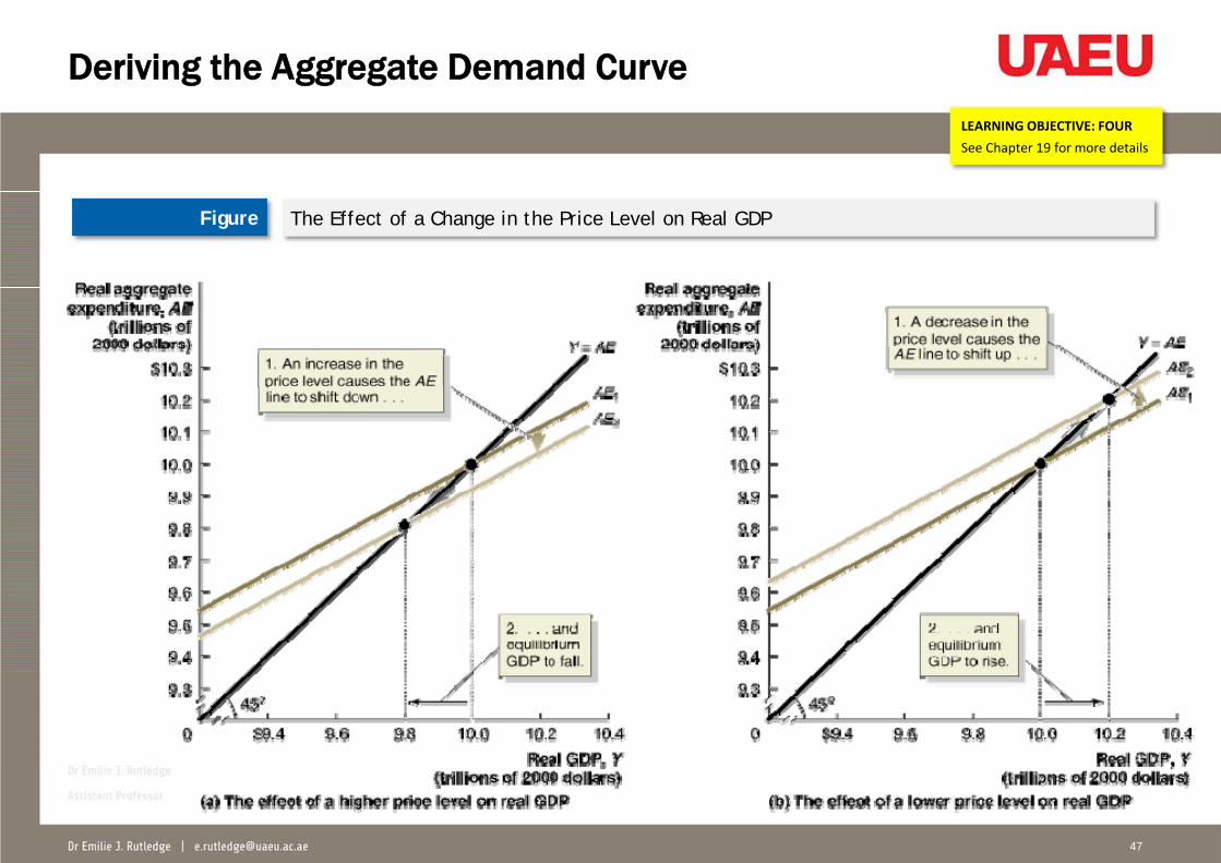
Deriving the Aggregate Demand CurveLEARNING OBJECTIVE: FOURSee Chapter 19 for more details

The Effect of a Change in the Price Level on Real GDPFigure

48

Aggregatedemandcurve:Acurvethatshowstherelationshipbetweenthepricelevelandthelevelofplannedaggregateexpenditureintheeconomy,holdingconstantallotherfactorsthataffectaggregateexpenditure.

The Aggregate Demand CurveLEARNING OBJECTIVE: FOURSee Chapter 19 for more details

The Aggregate Demand CurveFigure

49

Key Terms

» Aggregatedemandcurve

» AggregateExpenditure(AE)

» Aggregateexpendituremodel

» Autonomousexpenditure

» Cashflow

» Consumptionfunction

» Inventories

» MarginalPropensitytoConsume(MPC)

» MarginalPropensitytoSave(MPS)

» Multiplier

» Multipliereffect

short run output and expenditure - erutledge | arabian … · · 2014-04-13short-run output and...

Documents