short selling and the informational efficiency of prices
TRANSCRIPT

Short selling and the informational efficiency of prices
Ekkehart Boehmer J. (Julie) Wu ∗
This draft: January 5, 2009
ABSTRACT
We present direct empirical evidence that short sellers enhance the informational efficiency of prices. Using daily shorting flow data for a large panel of NYSE-listed stocks, we first show that greater shorting flow reduces deviations of transaction prices from a random walk. Second, at lower frequencies, we show that more shorting flow accelerates the incorporation of public information into prices. Third, greater shorting flow eliminates post-earnings announcement drift for negative earnings surprises. Fourth, we demonstrate that short sellers change their trading around large return events in a way that aids price discovery. These results are robust to various econometric methodologies and model specifications. Overall, our results highlight the important role that short sellers play in the price discovery process. Keywords: Informational efficiency of prices; Price discovery; Short selling JEL code: G14
∗ Ekkehart Boehmer, Department of Finance, Mays Business School, Texas A&M University, College Station, TX 77843-4218 ([email protected]). J. (Julie) Wu, Department of Banking and Finance, Terry College of Business, University of Georgia, Athens, GA 30602 ([email protected]). We thank Kerry Back, David Bessler, George Jiang, Sorin Sorescu, Heather Tookes and seminar participants at Texas A&M University and the 2007 FMA Doctoral Consortium for helpful comments.

Short selling and the informational efficiency of prices
The informational efficiency of prices is a critical issue in finance because it is a key attribute of
capital markets and can have important implications for the real economy.1 Efficiency is also a public
good, because all market participants benefit from more efficient prices. In this paper, we examine the
effect of daily short selling flow on informational efficiency. Our evidence suggests that short sellers play
an important role in the price discovery process and that their trading activity makes prices more
informationally efficient.
The consequences of short selling for market quality and the informational efficiency of share
prices is a hotly debated topic. While many academics agree that shorting helps price discovery, direct
evidence on this issue is scarce. This often allows arguments against short selling, frequently made by
issuers and regulators, to remain scientifically unanswered. Financial theory also allows different
predictions. In some models, short sellers are rational and informed traders who promote efficiency by
moving mispriced securities closer to their fundamentals (see, for example, Diamond and Verrecchia,
1987). In other models, short sellers may follow manipulative and predatory trading strategies, which
result in less informative prices (Goldstein and Guembel, 2008) or cause overshooting of prices
(Brunnermeier and Pedersen, 2005). Empirical studies on this issue also present mixed evidence. Most
studies suggest that short sellers are informed traders. Using either monthly short interest data (see, e.g.,
Desai, et al., 2002; Asquith, Pathak, and Ritter, 2005; Boehme, Danielsen, and Sorescu, 2006) or shorting
flow data (see, e.g., Christophe, Ferri, and Angel, 2004; Boehmer, Jones, and Zhang, 2008; Diether, Lee,
and Werner, 2007), these authors suggest that short sellers help correct overvaluation. But some
researchers argue that short sellers manipulate and destabilize prices around seasoned equity offerings
1 More efficient stock prices reflect more accurately a firm’s fundamentals and can guide firms in making better-informed investment and financing decisions. Related theoretical work focusing on the relation between informativeness of market prices and corporate decisions includes, among others, Tobin (1969), Dow and Gorton (1997), Subrahmanyam and Titman (2001), and Goldstein and Guembel (2008). Also related are recent empirical studies on seasoned equity offerings (Giammarino et al., 2004), mergers and acquisitions (Luo, 2005), and investments in general (Chen, Goldstein, and Jiang, 2006).
1

(Henry and Koski, 2007) or at times of large intraday illiquidity (Shkilko, Van Ness, and Van Ness,
2007).2
This paper is the first to take a more direct approach. Rather than measuring whether short sellers
anticipate future changes in returns or fundamentals, we relate publicly available daily shorting flow on
the NYSE directly to measures of informational efficiency. Compared to monthly snapshots of short
interest data that ignore intra-month shorting and covering of short positions, daily flow data can be a
significant improvement when some short sellers adopt short-term trading strategies. Indeed, recent
empirical evidence suggests that many short sellers are active short-term traders. Between November
1998 and October 1999, Reed (2007) finds that the median duration of a position in the equity lending
market is three days, and the mode is only one day. More recently, Diether, Lee, and Werner (2007)
estimate that the average days-to-cover for a shorted stock in 2005 is about four to five days. These
findings indicate that a large portion of recent short selling activity is short-term and even intradaily.3
Therefore, daily shorting flow data can overcome the potential limitation associated with monthly short
interest data, and enable researchers to investigate how shorting affects price efficiency at a high
frequency.
We use four distinct approaches to measure the effect of shorting on informational efficiency.
First, following Boehmer and Kelley (2009), we construct transaction-based high-frequency measures of
efficiency. Second, we adopt Hou and Moskowitz (2005)’s lower-frequency price-delay measure, which
estimates how quickly prices incorporate public information. Third, we use the well-established post-
earnings announcement drift anomaly (see Ball and Brown, 1968) to measure inefficiency and test
whether short sellers influence its magnitude. Fourth, we examine short selling around large price
movements and price reversals.
2 Anecdotal evidence also goes both ways. Jim Chanos, president of Kynikos Associates (the largest fund specializing in short selling), is best known as one of the first to spot problems with Enron. But recent high-profile lawsuits including Biovail, a Canadian pharmaceutical company suing hedge fund SAC, and Overstock.com suing Rocker Partners, accuse short sellers of manipulating their stock prices. 3 Jones (2003) documents an average of over 4% of daily trading volume for short sales established and covered in the same day in the early 1930s.
2

Our results uniformly indicate that short sellers improve the informational efficiency of prices.
First, more shorting flow reduces the deviation of transaction prices from a random walk, indicating that
more shorting makes prices more efficient. As one would expect, this result is more pronounced for those
stocks for which shorting constraints were relaxed between May 2005 and June 2007. Second, more
shorting flow is associated with fewer price delays, suggesting that prices incorporate public information
faster. Third, heavy shorting eliminates post-earnings announcement drift following large negative
earnings surprises. Fourth, we find no evidence that short sellers exacerbate large negative price shocks.
In contrast, their trading patterns seem to facilitate more accurate pricing even on extreme return days.
Our results are robust to different econometric methods and specifications and difficult to explain with
reverse causality. These findings suggest that short sellers play a critical role in facilitating rational price
discovery, a major function of capital markets.
We also provide some evidence on differential effects between informed and uninformed short
sellers. Theoretical models on short selling differentiate informed traders from uninformed traders (see,
for example, Diamond and Verrecchia, 1987; Bai, Chang, and Wang, 2006). While one cannot directly
distinguish between informed and uninformed short sellers, our data allow us to separately identify short
sales that are exempt from the Uptick Rule.4 These exempt transactions are less likely to be information
motivated, because they are primarily the result of market making activity. Indeed, we find that the
efficiency-enhancing effect that shorting flow has comes entirely from non-exempt short sellers, the
group that presumably is better informed than exempt traders. This finding supports our assertion that it is
short sellers’ information that helps make prices more efficient.
The key finding that daily shorting flow directly enhances the informational efficiency of share
prices contributes to the literature in a number of ways. First, it complements recent international studies
on the relation between short sales constraints and price efficiency. Bris, Goetzmann, and Zhu (2006)
4 The Uptick Rule, commonly known as the tick test, requires that short selling in exchange-listed stocks occur only at an uptick or a zero-plus tick. That is, short sales in these stocks need to transact above the last trade price or at the last trade price if the last trade price is higher than the most recent trade at a different price. See Rule 10a-1 under the Securities and Exchange Act of 1934.
3

conduct country-level analysis on short sales practices in 46 equity markets. They show that stock
markets where shorting is prevalent are slightly more efficient compared to countries where short selling
is prohibited, assuming that more efficient price discovery is associated with higher idiosyncratic risk and
less return comovement. Chang, Cheng, and Yu (2007) find that individual stock returns at the Hong
Kong stock market exhibit less positive skewness when short-sales restrictions are lifted, suggesting that
short sellers are helpful in incorporating bearish information into prices. Using weekly data from 26
markets on share lending supply and borrowing fees as proxies for short sales constraints, Saffi and
Sigurdsson (2007) show that less constrained firms are more efficiently priced in that they have shorter
price delays. Similarly, Reed (2007) finds that prices of severely short-sale constrained stocks deviate
more from their efficient value. In contrast to these studies, which focus on various types of short sale
constraints, our analysis examines the direct effect of actual shorting flow on the informational efficiency
of security prices.
Second, the direct efficiency-enhancing effect of shorting also extends indicative results in two
recent studies by Boehmer, Jones, and Zhang (2008) and Diether, Lee, and Werner (2007). Boehmer,
Jones, and Zhang (2008) use proprietary flow data on shorting for NYSE-listed stocks during 2000-2004,
and find that shorting flow is informative about future stock returns. They posit that “short sellers possess
important information and their trades are important contributors to more efficient prices.” Diether, Lee,
and Werner (2007), examining daily shorting flow for 2005, show that U.S. short sellers exhibit
contrarian trading behavior with respect to short-term past returns, and can also correctly predict future
negative returns. The authors conclude that “the evidence is consistent with short-sellers helping correct
short-term overreaction of stock prices to information.” Both papers stop at their conjectures, and do not
formally test whether there is a direct link between shorting flow and the informational efficiency of share
prices. Our analysis provides evidence of a direct connection between shorting and efficiency.
Third, short sellers’ efficiency-enhancing behavior around earnings announcement also adds to
the growing literature on post-earnings announcement drift initially documented in Ball and Brown
(1968). Although there is mounting evidence that post-earnings announcement drift is one of the most
4

persistent anomalies in financial markets, empirical work on shorting behavior in this context is quite
limited.5 We show that the arbitrage activity of short sellers leads to faster incorporation of information
into prices and consequently attenuates (or, in some cases, eliminates) the drift, further supporting a
positive role of short sellers in promoting efficient pricing.
The remainder of the paper is organized as follows. Section 1 describes the data and our sample.
Section 2 introduces our measures of relative informational efficiency. Section 3 analyzes the relation
between short selling and high-frequency measures of efficiency, while Section 4 looks at the relation
between shorting and low-frequency measures of efficiency. In Section 5 we describe our event-based
analysis that relates post-earnings announcements drift to shorting activity. In Section 6, we describe
several robustness tests and provide some evidence on causality. Section 7 concludes the paper.
1. Data and sample
The shorting flow data used in this paper are published by the NYSE as part of the requirements
under Regulation SHO and become first available in January 2005.6 This study covers the three-year
period up to December 2007.7 For each trade, the NYSE data include the size, if any, of the portion
transacted by short sellers and an indicator that identifies short sells that are exempt from the Uptick Rule.
Exempt shorts mainly result from (presumably uninformed) market-making activity or bona-fide arbitrage
transactions. For part of our analysis, we exploit differences between exempt and non-exempt shorting
flow.8 We aggregate shorting flow during normal trading hours into daily observations. One limitation of
5 Cao et al. (2007) only find relatively weak evidence that short sellers reduce drift, but their analysis uses monthly short interest data. Our tests use daily shorting flow data, which allows more powerful tests. 6 Regulation SHO initiated by the SEC aims to “study the effects of relatively unrestricted short selling on market volatility, price efficiency, and liquidity” (see Regulation SHO-Pilot Program (April 19 2005) at http://www.sec.gov/spotlight/shopilot.htm). 7 Reg SHO data end in June 2007. Comparable shorting data from July to December 2007 are directly obtained from the NYSE. 8 After the implementation of Reg SHO in January 2005, this classification is unambiguous only for non-pilot stocks. Among the pilot stocks, previously non-exempt orders may be marked “Exempt” in post-January 2005 pilot stocks; and some previously exempt short orders in pilot stocks may no longer be marked “Exempt” after January 2005. Specific examples of exempt shorting for market making purposes are sales by an odd-lot dealer or an exchange with which it is registered, or any over-the-counter sale by a third-market market maker who intends to offset customer odd-lot orders. The SEC defines the second category of exempt shorts, arbitrage shorting, as “an
5

these data, as with all previous studies of short selling, is the lack of information on when and how short
sellers cover their positions later on.
We match the NYSE daily shorting flow data with the Center for Research in Security Prices
(CRSP) data to obtain daily security-specific characteristics such as return, consolidated trading volume,
closing prices, and shares outstanding. We include only domestic common stocks (share codes 10 and 11)
in the analysis. We exclude stocks that trade above $999 during the sample period. Finally, we compute
daily liquidity and price efficiency measures from the NYSE’s Trades and Quotes (TAQ) data. Our final
sample includes a daily average of 1,361 stocks.
2. Measuring the relative informational efficiency of prices
We employ four different approaches to measure the relative informational efficiency of prices.
First, our most powerful tests focus on high-frequency measures of efficiency. We measure how close
transaction prices move relative to a random walk and conduct tests at the daily frequency to relate these
measures to short selling. Second, we use a longer-horizon measure based on weekly returns. These tests
consider the speed with which public information is incorporated into prices. Third, we exploit the well-
documented post-earnings announcement drift to study the effect of short selling in an event-based
context. If short selling improves efficiency, we expect the drift to be smaller when short sellers are more
active after negative earnings surprises. Fourth, we identify unusually large price changes that are later
reversed and look at short selling around these changes. Extreme price movements are useful in
evaluating the motivation for short selling, because they shed light on whether short sellers exacerbate
price swings or help to keep prices closer to the efficient values.
2.1. High-frequency informational efficiency
activity undertaken by market professionals in which essentially contemporaneous purchases and sales are effected in order to lock in a gross profit or spread resulting from a current differential in pricing” (see 17CFR240.10a-1).
6

We use two different measures to capture the relative efficiency of transaction prices, the pricing
error as suggested in Hasbrouck (1993) and the absolute value of intraday return autocorrelations. Both
measures are computed from intraday transactions or quote data and both capture temporary deviations
from a random walk, one way to describe an informationally efficient time series of prices. Recent
empirical evidence in Chordia, Roll, and Subrahmanyam (2005) supports this short-term view. Their
analysis suggests that “astute traders” monitor the market intently and most information is incorporated
into prices within 30 minutes through their trading activities. As a result, short-term efficiency measures
can best capture nature of temporary deviations from fundamental values.
We follow Hasbrouck (1993) in computing pricing errors (the Appendix provides details on
estimation). He decomposes the observed (log) transaction price, pt, into an efficient price (random walk)
component, mt, and a stationary component, the pricing error st. The efficient price is assumed to be non-
stationary and is defined as a security’s expected value conditional on all available information, including
public information and the portion of private information that can be inferred from order flow. The
pricing error, which measures the temporary deviation between the actual transaction price and the
efficient price, reflects information-unrelated frictions in the market (such as price discreteness, inventory
control effects, and other transient components of trade execution costs). To compute the pricing error, we
use all trades and execution prices of a stock. We estimate a Vector Auto Regression (VAR) model to
separate changes in the efficient price from transient price changes. Because the pricing error is assumed
to follow a zero-mean covariance-stationary process, its dispersion, σ(s), is a measure of its magnitude.
In our empirical analysis, we standardize σ(s) by the dispersion of intraday transaction prices, σ(p), to
control for cross-sectional differences in price volatility. Henceforth, this ratio σ(s)/σ(p) is referred to as
the “pricing error” for brevity. To reduce the influence of outliers, the dispersion of the pricing error is
required to be less than dispersion of intraday transaction prices.9
9 Boehmer, Saar, and Yu (2005) apply Hasbrouck's (1993) method to study the effect of the increased pre-trade transparency associated with the introduction of Openbook on the NYSE on stock price efficiency. Boehmer and Kelley (2009) find that institutions contribute to price efficiency using similar approaches. Hotchkiss and Ronen
7

Our second short-term measure of relative price efficiency is the absolute value of quote midpoint
return autocorrelations. The intuition is that if the quote midpoint is the market’s best estimate of the
equilibrium value of the stock at any point in time, an efficient price process implies that quote midpoints
follow a random walk. Therefore, quote midpoints should exhibit less autocorrelation in either direction
and a smaller absolute value of autocorrelation indicates greater price efficiency. To estimate quote
midpoint return autocorrelations, we choose a 30-minute interval (results are qualitatively identical for 5-
and 10-minute return intervals) based on the results from Chordia, Roll, and Subrahmanyam (2005). We
use |AR30| to denote the absolute value of this autocorrelation.
It is worth pointing out that pricing errors, by construction, only attribute information-unrelated
price changes to deviations from a random walk, whereas autocorrelations do not distinguish between
information-related and information-unrelated price changes. For example, splitting a large order by an
informed trader would produce a zero pricing error because prices change to reflect information from the
informed order flow, but it would generate a positive autocorrelation. In this regard, pricing errors are a
more sensible measure of the relative informational efficiency of prices.
2.2. Low-frequency informational efficiency
Hou and Moskowitz (2005) introduce price delays, an increasingly popular measure of relative
efficiency that relies on the speed of adjustment to market-wide information.10 Following their approach,
we compute weekly Wednesday-to-Wednesday returns for each stock. To estimate price delays, we
regress these returns on contemporaneous and four weeks of lagged market returns over one calendar
year. Then we estimate a second regression that restricts the coefficients on lagged market returns to zero.
The delay measure is calculated as 1 – [(R2 (restricted model) / R2 (unrestricted model)].11 Similar to an
F-test, this measure captures the portion of individual stock return variation that is explained by lagged
(2002) examine the informational efficiency of corporate bond prices using a simplified procedure suggested by Hasbrouck (1993). 10 See, for example, Griffin, Kelly, and Nardari (2007) and Saffi and Sigurdsson (2007). 11 To reduce noise, we do not compute this measure for stocks with fewer than 20 weekly returns during a calendar year.
8

market returns. The larger the delay, the less efficient the stock price is, in the sense that it takes longer
for the stock to incorporate market-wide information.
Relative to the high-frequency efficiency measures, a stock’s price delay captures informational
efficiency over a much longer horizon. Yet, the (untabulated) correlation between price delays and the
annual average of daily pricing errors is 0.33 and the correlation with |AR30| is 0.23, suggesting that these
measures also have common components.12
2.3. Post-earnings announcement drift
Post-earnings announcement drift is a well-established financial phenomenon that indicates some
degree of informational inefficiency in the capital markets. Ball and Brown (1968) first document that
abnormal returns of stocks with positive earnings surprises tend to remain positive for several weeks
following the earnings announcement, and remain negative for stocks with negative surprises. This return
pattern generates an arbitrage opportunity for savvy traders. If short sellers are sophisticated traders who
attempt to exploit this opportunity, we expect increased shorting immediately following negative earnings
surprises and decreased shorting following positive surprises. If short sellers make prices more
informationally efficient, the increased shorting activity following negative surprises should attenuate the
post-earnings announcement drift. We use this event-based test to supplement our previous two measures
of informational efficiency.
Battalio and Mendenhall (2005) and Livnat and Mendenhall (2006) show that earnings surprise
measures based on analyst forecasts are better than the ones obtained from a time series model of
(Compustat) earnings, because the former are not subject to issues such as earnings restatement and
special items. We compute earnings surprises as the difference between actual earnings and previous-
month I/B/E/S consensus forecasts, scaled by the stock price two days before the announcement date. We
12 Another potential low-frequency relative efficiency measure is the R2 from a market model regression as suggested in Morck, Yeung, and Yu (2000) and Durnev, et al. (2003). They argue that lower R2 indicates more firm-specific information and can thus be used as a measure of information efficiency of stock prices. However, recent work casts doubt on this interpretation and suggests that R2 does not capture information well (Kelly, 2005; Ashbaugh, Gassen, and LaFond, 2006; Griffin, Kelly, and Nardari, 2007; Saffi and Sigurdsson, 2007).
9

construct abnormal returns as a stock’s raw returns net of value-weighted market returns, and measure the
drift as the cumulative abnormal returns following each earnings surprise.
2.4. Return reversals
Opponents of unrestricted short selling often allege that short selling puts excess downward
pressure on prices.13 As a result, prices are claimed to be too low relative to fundamental values when
short sellers are active. A related allegation is that short sellers can manipulate prices by shorting
intensely, thereby driving prices down below their efficient values. Once these stocks are undervalued,
the short sellers could then cover their positions as the true valuations are slowly revealed and prices
reverse towards their efficient values. Both of these scenarios imply that short sellers are more active on
days when prices decline, and especially so when these declines are not related to fundamental
information. We provide evidence on this issue by selecting large price moves and looking at short
sellers’ behavior around these extreme return days.
3. Shorting flow and the short-term efficiency of transaction prices
Relative short-term efficiency describes how closely transaction prices follow a random walk,
and we estimate how short selling flow affects the degree of short-term efficiency. We regress daily
measures of short-term efficiency on lagged shorting and relevant control variables. Because the relevant
measures of efficiency and shorting are available at the daily frequency, these tests are quite powerful.
We use the following basic model to test hypotheses about short selling on efficiency:
Efficiencyi,t = α t + β t Shortingi,t-1 + γt Controlsi,t-1 + εi,t (1)
The dependent variable is either the pricing error, σ(s)/σ(p), or the absolute value of midquote return
autocorrelation, |AR30|. Daily shorting flow, the key variable of interest, is measured as a stock’s daily
shares sold short scaled by its daily share trading volume. This standardization makes shorting activity
comparable across stocks with different trading volume. If more shorting systematically contributes to
13 For public concerns or issuers’ comments, See SEC Release No. 34-58592, or NYSE survey on short selling (“Short selling study: The views of corporate issuers”, Oct 17, 2008).
10

greater price efficiency, stock prices should deviate less from a random walk, suggesting that β should be
negative. We lag explanatory variables by one period to mitigate any potential influence of changes in
price efficiency on these contemporaneous explanatory variables.14
Extant research suggests several control variables that are potentially associated with price
efficiency. We include measures of execution costs, share price, market capitalization, and trading
volume as controls in our base regressions. To measure execution costs, we use relative effective spreads
(measured as twice the distance between the execution price and the prevailing quote midpoint scaled by
the prevailing quote midpoint).15 Higher execution costs make arbitrage less profitable, and therefore
deter the entrance of sophisticated traders whose trading helps keep prices in line with their fundamentals.
This reasoning suggests that stocks with higher trading costs tend to deviate more from their fundamental
values, and thus are less efficiently priced. We include the volume-weighted average price (VWAP) to
control for differences in price discreteness that can potentially affect efficiency.16 Market capitalization
and trading volume are included to control for differences in firm size and trading activity, as larger and
more actively traded stocks may be easier to value.17 In addition, we include the lagged dependent
variable to control for potential persistence in relative price efficiency.18
Recent literature suggests two additional important variables that need to be considered in
studying price efficiency. First, because analyst coverage can improve a firm’s informational
environment, we control for the number of sell-side analysts (Brennan and Subrahmanyam, 1995). We
obtain the monthly number of analysts producing annual forecasts from I/B/E/S. Second, Boehmer and
Kelley (2009) find that institutional investors contribute to greater informational efficiency. We control 14 The lagged explanatory variables can be interpreted as instruments for their contemporaneous values. Results using contemporaneous values are qualitatively similar. 15 Controlling for relative effective spreads serves another purpose in the pricing error regression. The pricing error reflects the information-uncorrelated (i.e. temporary) portion of total price variance. Since the effective spread measures the total price impact of a trade and thus could conceivably be related to the pricing error, controlling for it can help isolate changes in efficiency from changes in liquidity. 16 Using closing prices produces qualitatively identical results. 17 The natural logs of trading volume and market capitalization have a correlation of 0.75. To mitigate this multicollinearity issue, we use residuals from regressing log of market capitalization on log volume in the reported regression results. Results remain qualitatively similar without this orthogonalization. 18 While price volatility is conceivably related to short-term efficiency, both of our dependent variables are already scaled by a volatility measure. Therefore, we do not add volatility as an explanatory variable to the model.
11

for institutional holdings so we can focus on marginal effect of shorting over and above the effect of
institutional holdings. As in Boehmer and Kelley, we use holdings from the 13F filings in the CDA
Spectrum database standardized by a firm’s shares outstanding.
3.1. Basic result
Panel A in Table 1 presents time-series means of cross-sectional summary statistics for these
variables. Relative shorting volume accounts for close to 20% of total trading volume during the sample
period. A 10% standard deviation reveals large variation in shorting activity across stocks. Price
efficiency measures also exhibit some cross sectional variations. Variables such as firm size, trading
volume, share prices, and number of analysts are skewed, and we their natural logarithms in our
estimation.
Panel B in Table 1 reports time-series averages of daily cross sectional correlations between
shorting and price efficiency. Pricing errors and |AR30| are positively correlated, but the correlation is
only moderate (0.07). This suggests that these two measures capture different aspects of price efficiency.
But shorting is negatively correlated with both price efficiency measures, providing initial evidence that
short selling is associated with greater relative price efficiency. Of course, these correlations are only
suggestive and we conduct more rigorous tests next to formalize this relation.
We employ a standard Fama and MacBeth (1973) two-step regression method to estimate model
(1). Specifically, we run daily cross-sectional regressions of price efficiency on shorting activity and draw
inferences from the time-series average of these regression coefficients. This method picks up the cross-
sectional effect of shorting on price efficiency, and is less affected by potential cross-sectional
correlations among regression errors than a pooled cross-sectional time series regression. To further
correct for potential autocorrelation in estimated coefficients, we use Newey-West standard errors with
five lags.19
Table 2 contains the regression results. Models 1 and 2 use pricing errors as the efficiency
measure, while models 3 and 4 use Ln|AR30|. For each measure, we present the base model and a model 19 Results are not sensitive to other reasonable lag lengths for Newey-West standard errors.
12

augmented by the number of analysts and institutional holdings. Lagged daily shorting flow has a
significant and negative coefficient in each of these specifications. This means that controlling for other
factors, higher shorting activity is associated with smaller pricing errors and smaller autocorrelation. In
other words, short selling is associated with prices that deviate less from a random walk, and hence are
more informationally efficient.
The coefficients of most control variables exhibit expected signs. Consistent with prior literature,
greater analyst coverage and more institutional holdings promote efficiency (Boehmer and Kelley, 2009).
As in their tests, we also find that larger relative effective spreads are associated with larger pricing
errors. This makes sense because higher spreads prevent some arbitrageurs from immediately jumping on
temporary price deviations, and therefore lead to lower efficiency. Finally, larger and more actively
traded stocks are also associated with smaller pricing errors.
3.2. The effect of less stringent shorting constraints during the Reg SHO pilot
In 2005, the SEC relaxes short selling constraints for a sample of “pilot” stocks. More
specifically, Reg SHO removes all price tests that prevent short sell orders from executing on downticks.
The less restricted short selling has no adverse effects on market quality but increases both the volume
and the aggressiveness of short selling (Diether, Lee, and Werner, 2008; Alexander and Pedersen, 2008).
In this sense, the pilot sample provides an interesting additional test of the relation between short selling
and price efficiency. In particular, price tests may limit the speed with which shorters’ information can
enter prices. Therefore, we would expect the efficiency-enhancing effect to be greater as restrictions on
short selling are relaxed.
To investigate this hypothesis, we use the same model as in Table 2 except that we allow
intercepts and the short selling slope coefficient to vary with changes in the uptick rule.20 More
specifically, we include four additional variables: a “pilot” dummy indicating pilot stocks; a “post”
dummy indicating the post-Reg SHO period over which price tests were removed for pilot stocks (i.e.
20 Because the Uptick Rule is eliminated on all stocks on July 6 2007, our sample for this analysis includes pilot stocks and control stocks from January 1, 2005 to July 5, 2007. For details on pilot and control stocks designation, see SEC Release No. 50104/July 28, 2004.
13

from May 2, 2005 onwards); an interaction pilot*post; and an interaction pilot*post*Shorting. Table 3
contains the results of this test and, as before, we report results for efficiency measured as Hasbrouck’s
pricing error (Models 1 and 2) and Ln|AR30| (Models 3 and 4).
The main results from Table 2 still hold. In particular, the total effect of short selling on price
efficiency (the sum of the coefficients on shorting and the interaction of shorting with the two dummy
variables) remains reliably negative across the different specifications. This means that shorting still
significantly increases future efficiency even when we control for the effects of the Reg SHO pilot.
Turning to the question of how the effect of shorting changes when the uptick rule is removed, however,
we find somewhat mixed results. The marginal effect of short selling does not change when efficiency is
measured as |AR30|, but it becomes more negative for the transaction-based pricing error. As predicted,
this suggests that (at least for pricing errors) removal of the uptick rule makes short selling a more
effective tool for keeping prices in line with their efficient values.
3.2. Exempt vs. non-exempt short selling
The analysis in the previous section lumps together all short sellers, but theoretical work on short
selling (Diamond and Verrecchia, 1987; Bai, Chang and Wang, 2006) models the behavior of informed
short sellers differently from that of uninformed short sellers. This section attempts to shed some light on
how different information is related to the effect shorting has on price efficiency.
While one cannot directly distinguish informed from uninformed short sellers, the NYSE shorting
data has a unique feature that helps differentiate, to some extent, different motivations for short selling.
Specifically, we observe an indicator that identifies shorts that are exempt from the Uptick Rule. Exempt
shorting primarily includes broker-dealer market-making activities and bona-fide arbitrage activities.
Shorting in the course of market making, by definition, should have less information content as shorting
by other traders. Similarly, arbitrage shorting relies on information about relative valuations rather than
information about the security itself. Other things equal, we thus expect non-exempt shorting to have a
stronger efficiency-enhancing effect than exempt shorting.
14

One technical issue complicates this test. After Reg SHO is implemented in May 2 2005, the
Uptick Rule ceases to apply for a subset of stocks (the “pilot stocks”).21 Reg SHO specifies that all short
sales in these pilot stocks should be marked as “exempt.” As a result, an “exempt” indicator in pilot
stocks does no longer unambiguously indicate market-making or arbitrage shorts as before. For these
reasons, our analysis in this section is limited to non-pilot stocks and ends on July 5, 2007.22
Table 4 presents summary statistics of exempt vs. non-exempt shorting for non-pilot stocks. Non-
exempt shorting clearly dominates total shorting activity on the NYSE. The mean (median) relative non-
exempt shorting, measured as non-exempt shorting volume scaled by total trading volume, accounts for
18% (16%) of total trading volume. Exempt shorting, measured as exempt shorting volume scaled by
total share volume, accounts for only 0.7% of total trading volume.
To investigate the differential effect of exempt vs. nonexempt shorting on the informational
efficiency of prices, we modify model (1) to include separate measure of exempt and non-exempt shorting
flow. Table 5 reports the Fama and MacBeth (1973) two-step regression results. We find that the
efficiency-enhancing effect of short selling is entirely attributable to non-exempt shorting. Stocks with
more intense non-exempt shorting have significantly smaller pricing errors and return autocorrelations.
Consistent with our conjecture, this suggests that non-exempt short selling is at least partially motivated
by information, and thus improves the informational efficiency of share prices. In contrast, exempt
shorting does not reduce pricing errors or the absolute value of return autocorrelations. Again, this
supports the conjecture that exempt shorting is not likely to be driven by information and thus contributes
little to price efficiency. Taken together, these results suggest that short sellers only improve the
informational efficiency of prices if their trades are information motivated. 21 The SEC selected pilot securities from Russell 3000 index as of June 25, 2004. First, 32 securities in the Russell 3000 index that are not listed on the American Stock Exchange (Amex), or on the New York Stock Exchange (NYSE), or not Nasdaq national market securities (NNM) are dropped. Securities that went public after April 30, 2004 are also excluded. The remaining securities are then sorted into three groups by marketplace, and ranked in each group based on average daily dollar volume over the one year prior to the issuance of the order. From each ranked group, SEC selected every third stock to be a pilot stock starting from the 2nd stock. The remaining stocks are suggested to be used as the control group where the price test restriction still applies. Of all pilot stocks, 50%, 2.2% and 47.8% are from NYSE, Amex, and Nasdaq NNM, respectively. For more information about Reg SHO, see SEC Release No. 50104/July 28, 2004 22 The SEC eliminated the Uptick Rule on all stocks on July 6 2007. See SEC Release No.34-55970.
15

4. Short selling flow and price delays
To substantiate the efficiency-enhancing effect of shorting based on the intraday approach, we
now examine how shorting affects price delays, a longer-term measure of informational efficiency. As
discussed earlier, price delays reflect the sensitivity of a firm’s returns to contemporaneous and lagged
market returns and measure how quickly market-wide information is incorporated into stock prices (Hou
and Moskowitz, 2005).
To make test results comparable to those in the main tests reported in Table 2, we include similar
control variables in the regression. The main difference is that due to the way this measure is constructed,
we observe price delays only at the annual frequency. Accordingly, we use annual averages of the control
variables in the estimation. Given the much shorter panel (with at most three observations for each stock),
we now adopt a pooled time-series cross-sectional regression procedure. 23
We report two regressions in Table 6, the base model and a model with the number of analysts
and institutional holdings added. We find that short selling has a significantly negative association with
price delays. This implies that stocks with more shorting activity incorporate public information
significantly faster into prices than those with less shorting. This finding substantiates the core result that
shorting enhances the informational efficiency of prices.
5. Short selling and post-earnings announcement drift
Post-earnings announcement drift is a well-known empirical finding that indicates some degree of
informational inefficiency. Since prices tend to drift upwards (downwards) following a positive (negative)
earnings shock, this predictable pattern creates a potential arbitrage opportunity for savvy traders. If short
sellers are sophisticated traders who attempt to exploit this opportunity, we expect more (less) shorting
immediately following negative (positive) earnings surprises. If short sellers enhance efficiency, the post-
23 We also include year dummies in the regression to control for potential time trends and the results remain similar.
16

earnings announcement drift should be attenuated accompanied by the increased shorting activity
following negative surprises. We use this event-based test to supplement our previous regression analysis.
Our sample covers 15,921 earnings announcement events. We use a simple portfolio approach to
examine how short sellers respond to earnings surprises. Specifically, each quarter, firms are sorted into
quartile portfolios according to the earnings surprise measures, with quartile 1 containing stocks with the
most negative surprises and quartile 4 those with the most positive surprises. In Panel A of Table 7, we
first check whether post-earnings announcement drift is present during our sample period. We report
cumulative abnormal returns associated with earnings announcements for each quartile. Throughout the
analysis in this section, we define abnormal returns as a stock’s raw returns net of value-weighted market
returns, and use equally-weighted portfolio returns. Consistent with prior findings, the announcement
effects are very strong: abnormal returns during the three-day window (-1, 1) centered on the
announcement date are highly negative (positive) for portfolios with extreme negative (positive) earnings
surprises. More importantly, post-earnings announcement drift is still present during the sample period:
prices of stocks with good (bad) surprises continue to drift upwards (downwards) after the announcement.
For example, one-week cumulative abnormal returns starting from the second day after the announcement
date (2, 6) increase monotonically from -0.73% for stocks with the most negative surprises to 0.42% for
stocks with the most positive surprises.
How do short sellers respond to these earnings shocks? If short sellers understand and seek to
exploit the arbitrage opportunity associated with post-earnings announcement drift, they would short
more intensively stocks in quartile 1 during and immediately after the announcement. In contrast, they
would reduce shorting activity in stocks in quartile 4. Panel B in Table 6 examines shorting activity from
two weeks before the announcement date to two weeks after the announcement, and Figure 1 plots these
shorting flows. From the Figure, we see that for stocks with very negative earnings surprises (quartile 1),
shorting increases significantly on the announcement date and during the following week. Compared to
shorting flow of 20.13% of trading volume one week before the announcement (-6, -2), shorting grows by
1.29% to 21.42% of trading volume during the week immediately following the announcement (2, 6).
17

This suggests that short sellers quickly become active in firms with negative earnings surprises,
apparently hoping to profit from further price declines in the future. In contrast, shorting activity in firms
with positive earnings surprises (quartile 4) decreases by 0.5% percent of volume during the week
following the announcements. This decrease indicates that short sellers retreat when they expect prices to
climb up in the future. These changes in shorting flow are statistically significant for the extreme quartiles
and are consistent with the hypothesis that short sellers seek to exploit this arbitrage opportunity.24
Arbitrage activities in financial markets facilitate efficient pricing. In the context of post-earnings
announcement drift, arbitrage behavior by informed short sellers should attenuate or even eliminate the
drift as short sellers quickly react to earnings surprises. Therefore, we expect smaller drift in stocks with
negative earnings shocks that are followed by intensified shorting and in stocks with positive surprises
that are followed by reduced shorting activity. To investigate this hypothesis, we conduct standard
double-sorted portfolio analysis. Each quarter, we sort stocks into quartiles based on earnings surprises.
Within each earnings surprise quartile, we partition stocks into two groups based on changes in shorting
activity around the announcement (i.e., average shorting during the one (or two) week(s) after the
announcement minus that during the one (or two) week(s) prior to the announcement).
Table 8 reports one- and two-week post-earnings announcement drift for this double sort. Again,
the evidence suggests that shorting enhances efficiency, in this case by reducing the drift. Using the one-
week drift, stocks with very negative earnings surprises accompanied with less shorting (cell Q1, Low)
still exhibit negative post-announcement drift of 1.54%. But stocks with intensified shorting (cell Q1,
High) have no drift: the return is -0.09% and not significantly different from zero. This suggests that short
sellers bring prices closer to fundamentals, in this context by eliminating the post-earnings announcement
drift associated with negative earnings surprises. Similarly, we observe significantly positive drift for
24 Although not the focus of this study, an interesting cross-sectional pattern in Figure 1 is that shorting activity preceding earnings announcement is generally higher (lower) in stocks with upcoming negative (positive) earnings surprises. This pattern seems to suggest that short sellers tend to be more active in firms that reported undesirable earnings in previous quarter(s) in anticipation of continued poor performance (Christophe, Ferri and Angel (2004), Desai, Krishnamurthy and Venkataraman (2006)). During the sample period, the first-order serial correlation of earnings surprises is (insignificantly) positive at 0.03.
18

stocks with positive surprises and increased shorting, but no drift for positive surprises associated with
reduced shorting activity. Using two-week drift produces almost identical results. Overall, these event-
based results provide additional support for the hypothesis that short sellers help make prices more
efficient.
5. Short selling and extreme price movements
In general, short sellers tend to be contrarians who sell more after periods of positive returns
(Diether, Lee, and Werner, 2007). But some studies also provide evidence that, under specific
circumstances, some short sellers can destabilize prices by driving prices away from efficient values. For
example, Shkilko, Van Ness, and Van Ness (2007) find that some short sellers drive down prices too far
during extreme price declines. Similarly, Henry and Koski (2007) argue that short sellers are able to push
prices too far down just before seasoned equity offerings. While the objective of our paper is to assess the
effect of short sellers as a group, rather than the subset who may exploit extreme return events or specific
corporate actions, it is useful to extend our analysis in this direction. More specifically, we look at short
selling around large price moves, and, in particular, around price reversals. Analysis of these extreme
events can also shed some light on the concern that short selling may cause “sudden and excessive
fluctuations of the prices.”25 If nefarious short sellers destabilize prices, we expect more intense shorting
on down days, especially when the downward price change is unrelated to fundamental information. In
contrast, if short sellers help to keep prices in line and close to their efficient values, we expect them to
short less on extreme down days and short more on extreme up days, especially when they are unrelated
to fundamental information.
To identify extreme return days for each stock, we select days with returns exceeding two
standard deviations, measured over the past 20 trading days. Then we classify these events into one of
four categories, depending on what happens on the next day: continuations, small reversals, large
reversals, and overshooting reversals. For example, if we have a large negative return on day t, a 25 See SEC Release No. 34-58592.
19

continuation is any non-positive return on day t+1. A reversal of less than 20% of the down-day’s return
would be classified as a small reversal, and one that reaches more than 20% but remains below the
closing price on day t-1 is a large reversal. An overshooting reversal means that the price on day t+1
closes above the closing price on day t-1. We proceed analogously for extreme positive returns events.
To make inferences about short sellers’ contributions to price discovery around these extreme
events, we exploit our ex-post knowledge that returns around reversals are at least partially transient.
Because information events would lead to permanent price adjustments, reversals tend to be unrelated to
information. For example, a large passive fund could experience outflows and be obliged to sell a larger
quantity of shares. This would temporarily lower prices to induce other traders to buy these shares. Once
the selling pressure subsides, prices would then return to the level prior to the large sell. If short sellers
are smart traders who understand that the initial negative return is temporary, we expect them to reduce
their shorting.while prices are (temporarily) below their efficient values. In contrast, for temporary
positive price shocks, we expect short sellers to increase shorting while prices are elevated. This
background allows us to make inferences without having to assume that short sellers trade on private
information about fundamental values. Instead, we make the weaker assumption that, conditional on
observing a large price change, they can distinguish information-based price changes from those that are
later reversed.
Figure 2 (extreme negative returns) and Figure 3 (extreme positive returns) summarize the
behavior of short sellers around these different return events. Each Figure contains four panels,
corresponding to the categories of price behavior on day t+1. We present results using daily raw returns,
but the graphs look very similar when we use market-adjusted returns to identify extreme return events
and subsequent price reactions. As before, we measure shorting as a percentage of contemporaneous
trading volume.
We first examine shorting around the large negative day t returns in Figure 2. The price drop
averages about 4-5% across the four panels. By construction, the shock in Panel A experiences a
continuation on the next day and we do not know if the returns are eventually reversed or not. We show
20

the continuation graphs for completeness. But because the negative returns in Panels B through D reverse
on the next day, we know that the corresponding t=0 returns are transient, and we can investigate whether
short sellers trade as if they understand that they are not information based. If shorters attempted to
manipulate prices or exacerbate price declines for these reversals, we would expect shorting to increase
either on the down day or before. None of the graphs supports this conjecture: shorting is fairly flat before
the drop and then declines dramatically on the day of the price decline. This suggests that short sellers, as
a group, recognize the price decline as temporary and reduce their selling activity accordingly. The
decrease in shorting alleviates downward pressure on prices and should result in smaller declines than we
would have observed had short sellers not changed their trading activity.
Next, we look at the day t+1 returns. In Panel A, these returns are negative; in all other panels,
they are positive and, by construction, these returns increase monotonically from Panel A to Panel D
relative to the day t price decline. If the extreme price declines on the previous day are temporary and
shorters interpret them correctly, we would expect shorting on day t+1 to increase with the magnitude of
the reversal. For example, if prices reverse partially (Panel B), informed short sellers may expect further
reversal and limit their trading activity. In contrast, we expect informed short seller to trade more
intensely during and after the overshooting reversals (Panel D). The day t+1 results support this
conjecture. In Panel A, price declines continue and shorting remains low. On days with small reversals
(Panel B), short selling increases slightly from day t, but remains substantially lower than before the
shock for the next five trading days. On days with large reversals (Panel C), short sellers resume their pre-
event activity level quickly. Finally, for the overshooting returns (Panel D), short sellers increase their
shorting activity the most. Notably, day t+1 shorting activity is monotonically related to the reversal
magnitude: we observe more short selling relative to pre-event means as we move from Panel A to Panel
D. Each of these observations is consistent with the view that short sellers trade to keep prices in line with
their efficient values.
Figure 3 repeats this analysis for the opposite event (extreme positive returns, further classified
into four categories according to t+1 returns). As we would expect for shorters who view the positive
21

return as transient, the day t price increases are always associated with a substantial increase in shorting
activity. This is consistent with the contrarian nature of short selling (see Diether, Lee, and Werner,
2007). Equally important, and similar to Figure 2, we find that shorting on day t+1 is monotonically
related to the magnitude of return reversals. Shorting is highest when prices continue to increase (Panel
A) and lowest when prices fall below their day t-1 level (Panel D).
Overall, these results are consistent with Diether, Lee, and Werner’s (2007) finding that short
sellers act as contrarians.26 In addition, we show that short sellers’ trading helps to accelerate price
discovery in these extreme events. Shorters sell more when prices jump unusually high, and they short
less when prices drop unusually low, and they swiftly change their behavior as prices reverse. Moroever,
for extreme returns that are reversed on the next day, short sellers appear to recognize the temporary
nature of these price swings. As a result, their trading provides liquidity to the market and keeps prices in
line, even during these volatile episodes.27
6. Robustness
Our key finding is that short sellers make prices more informationally efficient. We provide
evidence along four dimensions of efficiency by looking at the deviation of transaction prices from a
random walk, lower-frequency price delays, an event-based analysis of earnings announcement drift, and
shorting behavior around large price movements. In this section, we discuss additional evidence that
mostly relates to the high-frequency analysis in section 3.
26 Using a similar sample (largely the first half of our sample period), Shkilko, Van Ness, and Van Ness (2007) argue that short sellers worsen price declines. This seems to be at odds with the results we report in Figures 2 and 3. One potential reason for the difference is that Shkilko et al. look at 5-minute intraday cumulative returns. Another, more likely, reason is that they also use a different measure of shorting activity. Their measure weights shorting changes in the cross-section by the volatility of the stock-specific time series of short selling. Because the most informed shorting flow will tend to be the most volatile, their measure gives large weight to uninformed shorting and little weight to informed shorting. In this paper, in contrast, we weight equally across firms. In this sense, our results are not inconsistent with Shkilko et al.’s, because it is not surprising that the least informed short sellers do not improve efficiency. 27 Some issuers believe that short selling should be banned at volatile times. See “Short selling study: The views of corporate issuers”.
22

Shorting flow is highly skewed. To assure that no distributional issues affect our results, we use
decile ranks in place of shorting flow to test for efficiency effects. Specifically, on each day, we sort
stocks into deciles based on the prior day’s relative shorting volume. Then we use the decile ranks in
regression model (1). This approach reduces the influence of outliers on the estimates. Our main finding
remains unchanged with this alternative shorting measure: stocks ranked higher in terms of relative
shorting flow are associated with significantly smaller values of both pricing errors and return
autocorrelations. These results are not tabulated here.
Our high-frequency results may also be affected by firm-specific effects. To address this
possibility, we construct a measure of “abnormal” shorting. Each day, we compare a stock’s relative
shorting volume to its own moving average over the past week to determine whether shorting has become
more or less intense. This way we identify stocks that experience a shock in their own shorting activity
and take into account potential persistence in a firm’s shorting activity. For example, a large increase on a
day suggests abnormally high shorting relative to the prior week’s shorting activity. Again, we obtain
qualitatively identical results (not tabulated): stocks with higher abnormal shorting are priced more
efficiently as observed by smaller pricing errors and autocorrelations.
Another way of addressing stock fixed effects is to model them directly in a panel regression.
This methodology mitigates the omitted-variable concern with cross-sectional OLS regressions. Again,
the overall results from these panel regressions largely mirror the Fama-MacBeth estimates reported in
the text.
Finally, we address potential reverse causality. Institutional investors may prefer to hold
efficiently priced because they are less likely to be mispriced. But stocks with higher institutional
holdings are also easier to short, because the supply of lendable shares is greater. Therefore, efficiently
priced stocks may exhibit more shorting activity. If efficiency and shorting are sufficiently persistent, this
reverse-causality story could explain the association between efficiency and shorting flow. While we use
prior-day shorting in our analysis to mitigate this concern, we now address it more rigorously.
23

In the spirit of Granger causality tests, we regress time-series changes in efficiency on lagged
time-series changes in shorting for each stock, using the same set of control variables as in Table 2. We
require a stock to be actively traded for at least 45 days during the sample period to obtain reliable time-
series regression estimates. Table 9 reports the cross-sectional mean coefficients from these time-series
models. Panel A shows that greater increases in shorting are strongly associated with greater next-day
improvement in efficiency.
To examine reverse causality, we regress changes in shorting on lagged changes in price
efficiency, again using the same controls. Panel B in Table 9 shows that the average coefficient of the
lagged change in price efficiency, measured by either the pricing error or the absolute value of
autocorrelations, is not significantly related to changes in shorting. This indicates that changes in shorting
are not systematically related to past changes in price efficiency. While this exercise does not establish
causality, it is comforting that the time-series results closely parallel those from the cross-sectional
analysis and that they are not easily explainable using a reverse causality story.
7. Conclusions
We examine how daily short selling flow affects the informational efficiency of stock prices.
Using a range of efficiency measures, our evidence supports the idea that short sellers help to keep prices
in line with fundamentals. With more shorting, transaction prices more closely follow a random walk and
lower-frequency prices incorporate public information faster. We show that short sellers who are more
likely to trade on information have a greater efficiency-enhancing effect on prices, and this effect appears
to increase when shorting constraints are relaxed. Moreover, active short selling eliminates the well-
established post-earnings announcement drift following large negative earnings surprises and limits the
price distortions around large price changes. These results are fairly robust to different econometric
approaches and model specifications and we show that reverse causality explanations are hard to sustain.
Taken together, these different approaches all suggest that short sellers’ trading contributes
significantly to price discovery in equity markets. Short selling is associated with more efficient pricing in
24

the sense that prices appear to be closer to efficient or fundamental values when short sellers are more
active. In contrast, we find no evidence that hints at price destabilizing or manipulative trading by short
sellers.
We provide the first direct evidence on the effect that short selling has on pricing efficiency and
price discovery. Our results have important implications for recent regulatory actions that restrict short
selling. Specifically, restrictions on short selling constrain a particularly informed type of trading and are
likely to hamper the price-discovery function of equity markets.
25

APPENDIX
This appendix presents the estimation of the pricing error. The notations closely follow those in
Hasbrouck (1993). Hasbrouck assumes that the observed (log) transaction price at time t, pt, can be
decomposed into an efficient price, mt, and the pricing error, st:
pt = mt + st, (A.1)
where mt is defined as the security’s expected value conditional on all available information at transaction
time t. By definition, mt only moves in response to new information, and is assumed to follow a random
walk. The pricing error st measures the deviation relative to the efficient price. It captures non-
information related market frictions (such as price discreteness and inventory control effects, etc.). st is
assumed to be a zero-mean covariance-stationary process, and it can be serially correlated or correlated
with the innovation from the random walk of efficient prices. Because the expected value of the
deviations is zero, the standard deviation of the pricing error, σ(s), measures the magnitude of deviations
from the efficient price, and can be interpreted as a measure of price efficiency for the purpose of
assessing market quality.
In the empirical implementation, Hasbrouck (1993) estimates the following vector
AutoRegression (VAR) system with five lags:
tttttt
tttttt
vxdxdrcrcxvxbxbrarar
,222112211
,122112211
............
++++++=++++++=
−−−−
−−−− (A.2)
where rt is the difference in (log) prices pt, and xt is a column vector of trade-related variables: a trade
sign indicator, signed trading volume, and signed square root of trading volume to allow for concavity
between prices and trades. and are zero-mean, serially uncorrelated disturbances from the return
equation and the trade equation, respectively.
tv ,1 tv ,2
The above VAR can be inverted to obtain its vector moving average (VMA) representation that
expresses the variables in terms of contemporaneous and lagged disturbances:
............
2,21,2,22,11,1,1
2,21,2,22,11,1,1
*2
*1
*0
*2
*1
*0
*2
*1
*0
*2
*1
*0
+++++++=
+++++++=
−−−−
−−−−
ttttttt
ttttttt
vdvdvdvcvcvcxvbvbvbvavavar
( A.3)
26

To calculate the pricing error, only the return equation in (A.3) is used. The pricing error under
the Beveridge and Nelson (1981) identification restriction can be expressed as:
...... 1,21,201,11,10 +++++= −− ttttt vvvvs ββαα (A.4)
where , . ∑∞
+=
−=1
*
jkkj aα ∑
∞
+=
−=1
*
jkkj bβ
The variance of the pricing error is then computed as
[ ] ⎥⎦
⎤⎢⎣
⎡= ∑
∞
= j
j
jjjs vCov
βα
βασ )(,0
2)( (A.5)
In the estimation, all transactions in TAQ that satisfy certain criteria are included.28 Following
Hasbrouck (1993), I exclude overnight returns. I use Lee and Ready (1991) algorithm to assign trade
directions but make no time adjustment (Bessembinder (2003)). To make comparisons across stocks
meaningful, σ(s) is scaled by the standard deviation of pt, σ(p), to control for cross-sectional differences in
the return variance. This ratio σ(s)/σ(p) reflects the proportion of deviations from the efficient price in the
total variability of the observable transaction price process. Therefore, it serves as a natural measure of
the informational efficiency of prices. Because the pricing error is inversely related to price efficiency,
the smaller this ratio is, the more efficient the stock price is.29 In the empirical analysis, this ratio is
referred to as “pricing error” for brevity.
28 Trades and quotes during regular market hours are used. For trades, I require that TAQ’s CORR field is equal to zero, and the COND field is either blank or equal to *, B, E, J, or K. Trades with non-positive prices or sizes are eliminated. A trade with a price greater than 150% or less than 50% of the price of the previous trade is also excluded. For quotes, I include only those with positive depth for which TAQ’s MODE field is equal to 1, 2, 3, 6, 10, or 12. Quotes with non-positive ask or bid prices, or where the bid price is higher than the ask price are also excluded. A quote with the ask greater than 150% of the bid is also excluded. For each stock, I aggregate all trades during the same second that execute at the same price and retain only the last quote for every second if multiple quotes are reported. 29 As pointed out by Hasbrouck (1993), if temporary deviations from the efficient price take too long to correct, pricing errors will be understated because deviations are erroneously attributed to changes in efficient price. This potential limitation is not a major concern in this study for two reasons. First, my analysis examines the relative efficiency of prices instead of price efficiency in an absolute sense. Second, the empirical tests focus on the cross-section of stocks and this potential measurement error is unlikely to be highly systematic across stocks.
27

REFERENCES
Alexander, Gordon J. and Mark A. Peterson, 2008, The Effect of Price Tests on Trader Behavior and
Market Quality: An Analysis of Reg SHO," Journal of Financial Markets 11, 84-111.
Ashbaugh, Hollis, Joachim Gassen, and Ryan LaFond, 2006, Does stock price synchronicity represent
firm-specific information? The international evidence, Working paper, University of Wisconsin-
Madison.
Asquith, Paul, Parag A. Pathak, and Jay R. Ritter, 2005, Short Interest, Institutional Ownership, and Stock
Returns, Journal of Financial Economics 78, 243-76.
Bai, Yang, Eric C. Chang, and Jiang Wang, 2006, Asset prices under short-sale constraints, Working
paper, MIT.
Ball, Ray, and Philip Brown, 1968, An Empirical Evaluation of Accounting Income Numbers, Journal of
Accounting Research 6, 159-178.
Battalio, Robert, and Richard Mendenhall, 2005, Earnings expectations, investor trade size, and
anomalous returns around earnings announcements, Journal of Financial Economics 77, 289-319.
Bessembinder, Hendrik, 2003, Issues in Assessing Trade Execution Costs, Journal of Financial Markets
6, 233-57.
Beveridge, Stephen, and Charles R. Nelson, 1981, A New Approach to Decomposition of Economic Time
Series into Permanent and Transitory Components with Particular Attention to Measurement of
the Business Cycle, Journal of Monetary Economics 7, 151-74.
Boehme, Rodney D, Bartley R Danielsen, and Sorin M Sorescu, 2006, Short-Sale Constraints,
Differences of Opinion, and Overvaluation, Journal of Financial and Quantitative Analysis 41,
455-487.
Boehmer, Ekkehart, Charles M. Jones, and Xiaoyan Zhang, 2008, Which Shorts are Informed?, Journal
of Finance 63, 491-527.
Boehmer, Ekkehart, and Eric Kelley, 2009, Institutional Investors and the Informational Efficiency of
Prices, Review of Financial Studeis, forthcoming.
28

Boehmer, Ekkehart, Gideon Saar, and Lei Yu, 2005, Lifting the Veil: An Analysis of Pre-trade
Transparency at the NYSE, Journal of Finance 60, 783-815.
Brennan, Michael, and Avanidhar Subrahmanyam, 1995, Investment Analysis and Price Formation in
Securities Markets, Journal of Financial Economics 38, 361-381.
Bris, Arturo, William N. Goetzmann, and Ning Zhu, 2006, Efficiency and the bear: short sales and
markets around the world, Journal of Finance, forthcoming.
Brunnermeier, Markus K., and Lasse Heje Pedersen, 2005, Predatory Trading, Journal of Finance 60,
1825-1863.
Cao, Bing, Dan Dhaliwal, Adam C. Kolasinski, and Adam V. Reed, 2007, Bears and Numbers:
Investigating how short sellers exploit and affect earnings-based pricing anomalies, Working
paper, University of Washington.
Chang, Eric C., Joseph W. Cheng, and Yinghui Yu, 2007, Short-Sales Constraints and Price Discovery:
Evidence from the Hong Kong Market, Journal of Finance, forthcoming.
Chen, Qi, Itay Goldstein, and Wei Jiang, 2006, Price Informativeness and Investment Sensitivity to Stock
Price, Review of Financial Studies Forthcoming.
Chordia, Tarun, Richard Roll, and Avanidhar Subrahmanyam, 2005, Evidence on the speed of
convergence to market efficiency, Journal of Financial Economics forthcoming.
Christophe, Stephen E., Michael G. Ferri, and James J. Angel, 2004, Short-Selling Prior to Earnings
Announcements, Journal of Finance 59, 1845-75.
Desai, Hemang, Srinivasan Krishnamurthy, and Kumar Venkataraman, 2006, Do Short Sellers Target
Firms with Poor Earnings Quality? Evidence from Earnings Restatements, Review of Accounting
Studies 11, 71-90.
Desai, Hemang, K. Ramesh, S. Ramu Thiagarajan, and Bala V. Balachandran, 2002, An Investigation
of the Informational Role of Short Interest in the Nasdaq Market, Journal of Finance 57, 2263-
87.
29

Diamond, Douglas W., and Robert E. Verrecchia, 1987, Constraints on Short-Selling and Asset Price
Adjustment to Private Information, Journal of Financial Economics 18, 277-311.
Diether, Karl B., Kuan-Hui Lee, and Ingrid M. Werner, 2007, Short-Sale Strategies and Return
Predictability, Review of Financial Studies, forthcoming.
Diether, Karl B., Kuan-Hui Lee, and Ingrid M. Werner, 2008, It’s SHO Time! Short-Sale Price-Tests and
Market Quality, Journal of Finance, forthcoming.
Dow, James, and Gary Gorton, 1997, Stock Market Efficiency and Economic Efficiency: Is There a
Connection?, Journal of Finance 52, 1087-1129.
Durnev, Art, Randall Morck, Bernard Yeung, and Paul Zarowin, 2003, Does Greater Firm-Specific
Return Variation Mean More or Less Informed Stock Pricing?, Journal of Accounting Research
41, 797-836.
Fama, Eugene F., and James D. MacBeth, 1973, Risk, Return and Equilibrium: Empirical Tests, Journal
of Political Economy 71, 607-636.
Giammarino, Ronald, Robert Heinkel, Burton Hollifield, and Kai Li, 2004, Corporate Decisions,
Information and Prices: Do Managers Move Prices or Do Prices Move Managers?, Economic
Notes 33, 83-110.
Goldstein, Itay, and Alexander Guembel, 2008, Manipulation and the allocational role of prices, Review
of Economic Studies 75, 133-164.
Griffin, John M., Patrick J. Kelly, and Federico Nardari, 2007, Measuring Short-Term International Stock
Market Efficiency, Working paper, University of Texas at Austin.
Hasbrouck, Joel, 1993, Assessing the Quality of a Security Market: A New Approach to Transaction-Cost
Measurement, Review of Financial Studies 6, 191-212.
Henry, Tyler, and Jennifer Koski, 2007, Short Selling Around Seasoned Equity Offerings, Working
paper, University of Georgia.
Hotchkiss, Edith S., and Tavy Ronen, 2002, The Informational Efficiency of the Corporate Bond Market:
An Intraday Analysis, Review of Financial Studies 15, 1325-1354.
30

31
Hou, Kewei, and Tobias J. Moskowitz, 2005, Market Frictions, Price Delay, and the Cross-Section of
Expected Returns, Review of Financial Studies 18, 981-1020.
Jones, Charles M., 2003, Shorting Restrictions, Liquidity, and Returns, Working paper, Columbia
University.
Kelly, Patrick J., 2005, Information Efficiency and Firm-Specific Return Variation, Working paper,
University of South Florida.
Lee, Charles M C, and Mark J Ready, 1991, Inferring Trade Direction from Intraday Data, Journal of
Finance 46, 733-746.
Livnat, Joshua, and Richard Mendenhall, 2006, Comparing the Post–Earnings Announcement Drift for
Surprises Calculated from Analyst and Time Series Forecasts, Journal of Accounting Research
44, 177-205.
Luo, Yuanzhi, 2005, Do Insiders Learn from Outsiders? Evidence from Mergers and Acquisitions Journal
of Finance 60, 1951-1982.
Morck, Randall, Bernard Yeung, and Wayne Yu, 2000, The Information Content of Stock Markets: Why
Do Emerging Markets Have Synchronous Stock Price Movements?, Journal of Financial
Economics 58, 215-260.
Reed, Adam V., 2007, Costly Short-selling and Stock Price Adjustment to Earnings Announcements,
Working paper, University of North Carolina at Chapel Hill.
Saffi, Pedro A., and Kari Sigurdsson, 2007, Price Efficiency and Short-Selling, Working paper, London
Business School.
Shkilko, Andriy, Bonnie Van Ness, and Robert Van Ness, 2007, Price-destablizing Short Selling,
Working paper, Wilfrid Laurier University.
Subrahmanyam, A., and Sheridan Titman, 2001, Feedback from Stock Prices to Cash Flows, Journal of
Finance 56, 2389-2413.
Tobin, James, 1969, A General Equilibrium Approach To Monetary Theory, Journal of Money, Credit
and Banking 1, 15-29.

Variable Mean Median StdDevσ(s)/σ(p) 0.0946 0.0622 0.1039|AR30| 0.2478 0.2176 0.1767Shorting 19.75% 18.38% 9.92%RES 0 0011 0 0007 0 0012
Table 1. Summary Statistics
The sample includes a daily average of 1,361 NYSE-listed common stocks from Jan 2005 to Dec 2007. Panel A reports time-series means of daily cross-sectional summary statistics. σ(s) is the standard deviation of the discrepancies between logtransaction price and the efficient price based on Hasbrouck (1993). σ(p) is the standard deviation of intraday transaction prices.|AR30| is the absolute value of the 30-minute quote midpoint return autocorrelation. Shorting is calculated as shares shortedstandardized by trading volume on a given stock day. Volume is daily share trading volume expressed in millions. RES is dailyvolume-weighted relative effective spreads. VWAP is daily volume-weighted average price. Price is a stock's daily closing price.Size is the market value of equity expressed in billions of dollars. InstOwn is the fraction of shares outstanding owned by
institutions. NumAnalyst is the number of sell-side analysts producing annual forecast of firm earnings. Panel B reports the time-series averages of cross-sectional correlations between shorting and efficiency measures, where efficiency refers to σ(s)/σ(p) or|AR30|. Numbers in boldface indicate significance at 0.05 level.
32
RES 0.0011 0.0007 0.0012Size ($billions) 8.808 2.185 25.479VWAP($) 36.39 31.91 25.25Price($) 36.42 31.90 25.31Volume (millions) 1530.893 542.210 3639.900InstOwn 69.9% 75.1% 21.5%NumAnalyst 10 8 6
Panel B: Correlation between shorting and efficiencyσ(s)/σ(p) |AR30| Shorting
σ(s)/σ(p) 1.000|AR30| 0.073 1.000Shorting -0.055 -0.014 1.000
32

Coef p Coef p Coef p Coef pIntercept 0.2578 0.00 0.2476 0.00 -1.6102 0.00 -1.5910 0.00LagShorting -0.0597 0.00 -0.0438 0.00 -0.0751 0.00 -0.0926 0.00L L VWAP 0 0137 0 00 0 0122 0 00 0 0113 0 00 0 0101 0 00
Model 1 Model 2 Model 3 Model 4
Table 2. Fama-MacBeth Regressions of Price Efficiency on Shorting
This table reports daily Fama-MacBeth regression results for NYSE-listed common stocks from Jan 2005 to Dec 2007. σ(s) is the standarddeviation of the discrepancies between log transaction price and the efficient price based on Hasbrouck (1993). σ(p) is the standarddeviation of intraday transaction prices. |AR30| is the absolute value of the 30-minute quote midpoint return autocorrelation. Shorting isshares shorted standardized by shares traded on a given stock day. RES is daily value-weighted relative effective spreads. VWAP is dailyvolume-weighted average price. Size is the market value of equity. Volume is orthogonalized daily share trading volume with respect tosize. DV is the dependent variable. InstOwn is the fraction of shares outstanding owned by institutions. NumAnalyst*100 is the number ofsell-side analysts producing annual forecast of firm earnings (scaled up by 100). Lag indicates a value lagged by one day. Ln refers to thenatural logarithm. p value is based on Newey-West standard errors adjusted for 5 lags.
σ(s)/s(p) σ(s)/σ(p) Ln|AR30| Ln|AR30|
33
LagLnVWAP -0.0137 0.00 -0.0122 0.00 -0.0113 0.00 -0.0101 0.00LagLnsize -0.0108 0.00 -0.0087 0.00 -0.0078 0.00 -0.0046 0.01LagLnVolume -0.0191 0.00 -0.0145 0.00 -0.0115 0.00 -0.0127 0.00LagRES 16.8383 0.00 17.6646 0.00 -3.2536 0.00 -2.2286 0.16LagDV 0.4432 0.00 0.4021 0.00 0.0043 0.00 0.0040 0.00LagInstOwn -0.0223 0.00 -0.0033 0.70LagLnNumAnalyst*100 -0.0020 0.00 -0.0098 0.00
33

Dependent variable σ(s)/σ(p) t σ(s)/σ(p) t Ln|AR30| t Ln|AR30| tModel 1 Model 2 Model 3 Model 4
Coef. p Coef. p Coef. p Coef. pIntercept 0.3500 0.00 0.3843 0.00 -1.6060 0.00 -1.5897 0.00Shorting t-1 -0.0270 0.00 -0.0200 0.00 -0.1011 0.00 -0.1027 0.00Pilot -0.0024 0.21 -0.0006 0.70 -0.0034 0.66 0.0028 0.73Post 0.0030 0.00 0.0032 0.00 -0.0110 0.02 -0.0067 0.18Pilot*Post 0.0059 0.00 0.0049 0.00 0.0083 0.41 0.0039 0.72Pilot*Post*Shorting t-1 -0.0241 0.00 -0.0206 0.00 0.0054 0.86 -0.0070 0.83L V l 0 0085 0 00 0 0075 0 00 0 0094 0 00 0 0086 0 00
Table 3. Reg SHO and Price EfficiencyThis table reports results for a daily random effects panel estimation for pilot and control stocks listed on the NYSEduring the period from January 2005 to July 5 2007. σ(s) is the standard deviation of the discrepancies between logtransaction price and the efficient price based on Hasbrouck (1993). σ(p) is the standard deviation of intradaytransaction prices. |AR30| is the absolute value of the 30-minute quote midpoint return autocorrelation. Shorting isshorting volume scaled by trading volume. Volume, RES, VWAP, and Size are daily share trading volume, trade-weighted relative effective spreads, volume-weighted average prices, and market value of equity, respectively. Pilot isa dummy variable equal to one for pilot stocks and zero for control stocks. Post is a dummy variable equal to one after5/2/2005 and zero before that date. InstOwn is the fraction of shares outstanding owned by institutions.NumAnalyst*100 is the number of sell-side analysts producing annual forecast of firm earnings (scaled up by 100).DV is the dependent variable. t indexes trading day t. Ln refers to the natural logarithm.
34
LnVolume t-1 -0.0085 0.00 -0.0075 0.00 -0.0094 0.00 -0.0086 0.00RES t-1 3.1226 0.00 3.2857 0.00 5.2733 0.01 3.3070 0.22lnVWAP t-1 -0.0048 0.00 -0.0043 0.00 -0.0043 0.20 -0.0048 0.21LnSize t-1 -0.0106 0.00 -0.0087 0.00 -0.0014 0.51 0.0016 0.57DV t-1 0.2999 0.00 0.2565 0.00 0.0028 0.02 0.0032 0.01LnInstOwn t-1 -0.0461 0.00 -0.0070 0.51LnNumAnalyst*100 t-1 -0.0067 0.00 -0.0098 0.00
34
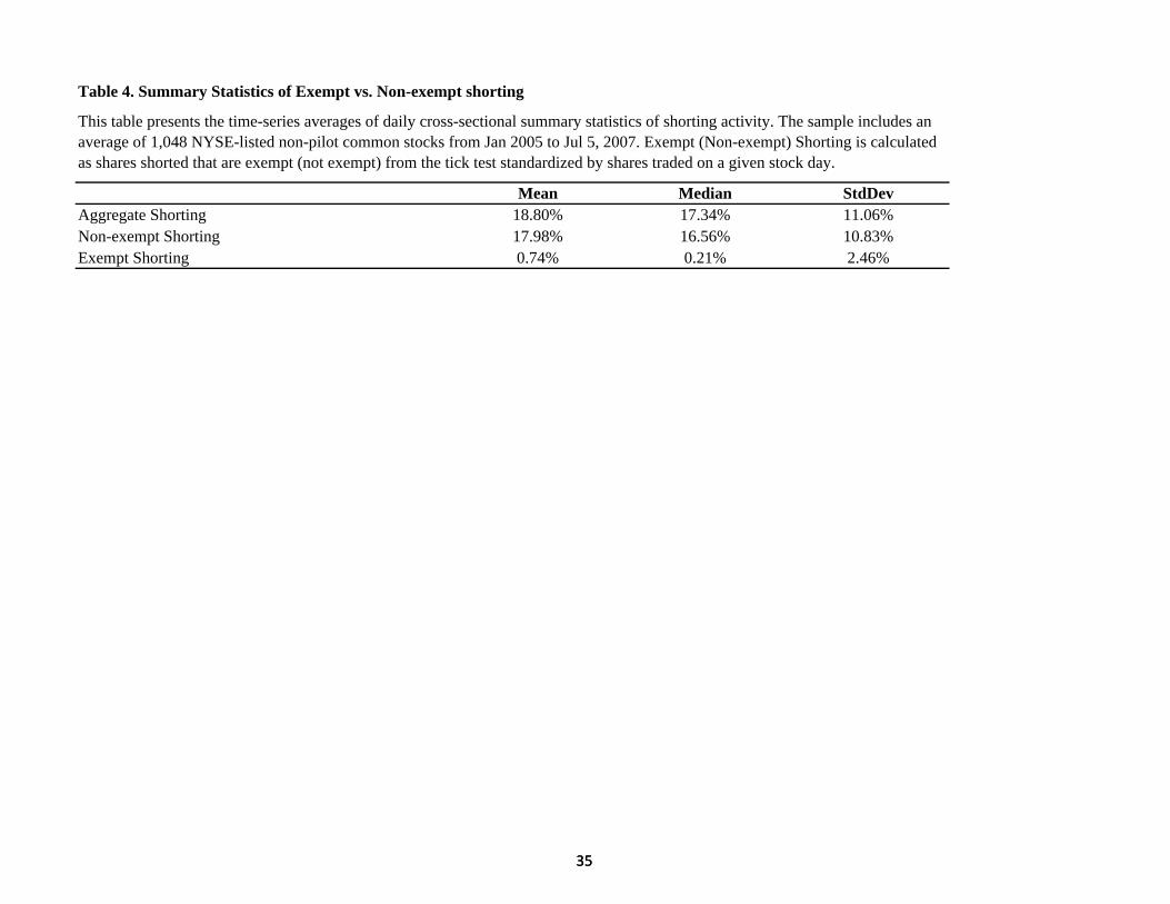
Mean Median StdDevAggregate Shorting 18.80% 17.34% 11.06%Non-exempt Shorting 17.98% 16.56% 10.83%Exempt Shorting 0.74% 0.21% 2.46%
Table 4. Summary Statistics of Exempt vs. Non-exempt shorting
This table presents the time-series averages of daily cross-sectional summary statistics of shorting activity. The sample includes an average of 1,048 NYSE-listed non-pilot common stocks from Jan 2005 to Jul 5, 2007. Exempt (Non-exempt) Shorting is calculated as shares shorted that are exempt (not exempt) from the tick test standardized by shares traded on a given stock day.
3535

Coef p Coef p Coef p Coef pIntercept 0.2897 0.00 0.2701 0.00 -1.6008 0.00 -1.5541 0.00LagNon-exempt Shorting -0.0581 0.00 -0.0376 0.00 -0.0712 0.00 -0.0912 0.00
Model 1 Model 2 Model 3 Model 4
Table 5. Fama-MacBeth Regression of Price Efficiency on Exempt vs. Non-exempt Shorting
This table reports daily Fama-MacBeth regression results for NYSE-listed non-pilot common stocks during the sample period from Jan2005 to Jul 5 2007. σ(s) is the standard deviation of the discrepancies between log transaction price and the efficient price based onHasbrouck (1993). σ(p) is the standard deviation of intraday transaction prices. |AR30| is the absolute value of the 30-minute quotemidpoint return autocorrelation. Exempt (Non-exempt) Shorting is calculated as shorted shares that are exempt (not exempted) from thetick test standardized by shares traded on a given stock day. RES is daily value-weighted relative effective spreads. VWAP is daily volume-weighted average price. Size is the market value of equity. Volume is orthogonalized daily share trading volume with respect to size. DV isthe dependent variable. InstOwn is the fraction of shares outstanding owned by institutions. NumAnalyst*100 is the number of sell-sideanalysts producing annual forecast of firm earnings (scaled up by 100). Lag indicates a value lagged by one day. Ln refers to the naturallogarithm. p value is based on Newey-West standard errors adjusted for 5 lags.
σ(s)/σ(p) σ(s)/σ(p) Ln|AR30| Ln|AR30|
36
LagExempt Shorting 0.0495 0.01 -0.0095 0.62 -0.0491 0.78 -0.4809 0.09LagLnVWAP -0.0158 0.00 -0.0147 0.00 -0.0146 0.00 -0.0114 0.01LagLnsize -0.0124 0.00 -0.0092 0.00 -0.0080 0.00 -0.0042 0.05LagLnVolume -0.0213 0.00 -0.0160 0.00 -0.0104 0.00 -0.0109 0.00LagRES 17.1455 0.00 18.1358 0.00 -3.8911 0.00 -3.6290 0.05LagDV 0.4292 0.00 0.3878 0.00 0.0045 0.00 0.0042 0.00LagInstOwn -0.0232 0.00 -0.0110 0.28LagLnNumAnalyst*100 -0.0028 0.00 -0.0153 0.00
36

Table 6. Regression of Price Delays on Shorting
Coef p Coef pIntercept 0.9170 0.00 0.8782 0.00Shorting -0.5699 0.00 -0.5605 0.00LnVWAP -0.0218 0.03 -0.0179 0.16LnSize -0.0317 0.00 -0.0446 0.00LnVolume -0.0108 0.09 -0.0131 0.14RES 3.7518 0.31 2.2198 0.68lagDV 0.1433 0.00 0.1208 0.00
This table reports pooled time-series cross sectional regression results for NYSE-listed common stocksfrom Jan 2005 to Dec 2007. The dependent variable is price delays estimated as in Hou and Moskowitz(2005). Shorting is the annual average of daily shares shorted standardized by shares traded. RES is theannual average of daily value-weighted relative effective spreads. VWAP is the annual average of dailyvolume-weighted average price. Size is the annual average of a firm's market value of equity. Volume isorthogonalized annual average of daily share trading volume with respect to annual average size. DV isthe dependent variable. InstOwn is the annual average of fraction of shares outstanding owned byinstitutions. NumAnalyst*100 is the annual average of number of sell-side analysts producing annualforecast of firm earnings (scaled up by 100). Ln refers to the natural logarithm. Lag refers to the first-order lagged value.
Price Delay Price DelayModel 1 Model 2
37
lagDV 0.1433 0.00 0.1208 0.00InstOwn -0.0335 0.26LnNumAnalyst*100 0.0372 0.00
37

Table 7. Earnings announcement returns, post-earnings announcement drift and short selling activity
Panel A. Cumulative abnormal returns around earnings announcements sorted on earnings surprises[-1, 1] [2, 6] [2, 11]
Earnings surpriseQ 1 (most negative) -3.18% *** -0.73% *** -0.77% *** t-stat -27.57 -8.38 -6.36Q2 -0.73% *** -0.20% *** -0.27% *** t-stat -7.23 -3.25 -3.49Q3 1.50% *** 0.01% -0.07% t-stat 17.78 0.17 -0.85
This table presents cumulative abnormal returns and shorting activity around quarterly earnings announcements. Each quarter, stocks are sorted into quartiles according to earnings surprises (calculated as the difference between the actual number and analyst concensus, scaled by stock prices two days prior to the announcement). Panel A reports market-adjusted cumulative abnormal returns around quarterly earnings announcements. Columns [-1, 1], [2, 6], and [2, 11] represent periods relative to the earnings announcement date (0). Panel B reports daily average relative shorting volume around earnings announcements. Columns [-11, 2], [-6, 2], [-1, 1], [2, 6], and [2, 11] represent periods relative to the earnings announcement date (0). Asterisks *, **, *** represents significance at 0.1, 0.05, and 0.01 level respectively.
38
Q4 (most positive) 3.36% *** 0.42% *** 0.44% *** t-stat 32.39 5.62 4.57
Panel B. Average shorting around earnings announcements[-11, -2] [-6, -2] [-1, 1] [2, 6] [2, 11] [2, 6] - [-6, -2] [2, 11] -[-11, -2]
Earnings surpriseQ1 (most negative) 20.19% 20.13% 20.48% 21.42% 21.24% 1.29% *** 1.03% ***Q2 20.03% 19.93% 20.01% 20.25% 20.13% 0.28% *** 0.06%Q3 19.54% 19.46% 19.53% 19.32% 19.32% -0.15% -0.23% **Q4 (most positive) 19.57% 19.49% 19.12% 18.97% 18.92% -0.54% * -0.67% ***
38

Table 8. Post-earnings announcement drift of portfolios double sorted on earnings surprises and changes in shorting activity
Post-earnings announcement drift [2,6] Post-earnings announcement drift [2,11]Change in shorting Change in shorting
low high low highEarnings surprise
Q1(most negative) ‐1.54% *** ‐0.09% -1.75% *** 0.01% t-stat -10.86 -0.85 -8.96 0.05Q2 ‐0.77% *** 0.37% *** -0.89% *** 0.35% ***
t t t 8 20 4 61 7 86 3 26
This table reports mean post-earnings announcement drift of firms sorted on earnings surprises and changes in shorting activity around earnings announcements. Each quarter, stocks are sorted into quartiles according to earnings surprises (calculated as the difference between the actual number and analyst concensus, scaled by stock prices two days prior to the announcement), and then split into two groups based on the median change in average shorting from one week before to one week after the announcement. The drift is calculated as market-adjusted cumulative abnormal returns. Asterisks *, **, *** represent significance at 0.1, 0.05, and 0.01 level respectively.
39
t-stat -8.20 4.61 -7.86 3.26Q3 ‐0.56% *** 0.61% *** -0.75% *** 0.66% *** t-stat -6.76 7.44 -6.80 5.97Q4 (most positive) ‐0.11% 1.04% *** 0.11% 0.82% *** t-stat -1.07 9.62 0.85 5.75
39

Table 9. Granger causality tests of changes in price efficiency and changes in shorting activity
Panel A: Dependent variable is change in price efficiency (ΔEfficiency)
Coef p Coef p Coef p Coef pIntercept 0.0004 0.00 -0.0001 0.69 0.0003 0.29 -0.0001 0.90Lag ΔEfficiency -0.4720 0.00 -0.4732 0.00 -0.4977 0.00 -0.4971 0.00Lag ΔShorting -0.0095 0.00 -0.0090 0.00 -0.0576 0.01 -0.0651 0.01L ΔL VWAP 0 0 84 0 18 0 0686 0 3 0 3 3 0 10 0 3 96 0 1
Δσ(s)/σ(p) Δσ(s)/σ(p) ΔLn|AR30| ΔLn|AR30|Model 1 Model 2 Model 3 Model 4
This table reports cross-sectional averages of time-series granger causality regression results for NYSE-listed common stocks from Jan 2005 to Dec 2007. σ(s) is the standard deviation of the discrepancies between log transaction price and the efficient price based on Hasbrouck (1993). σ(p) is the standard deviation of intraday transaction prices. |AR30| is the absolute value of the 30-minute quote midpoint return autocorrelation. Shorting is shares shorted standardized by shares traded on a given stock day. VWAP is daily volume-weighted average price. Size is the market value of equity. Volume is daily share trading volume. RES is daily value-weighted relative effective spreads. InstOwn is the fraction of shares outstanding owned by institutions. NumAnalyst*100 is the number of sell-side analysts producing annual forecast of firm earnings (scaled up by 100). Ln represents the natural logarithm. Δ indicates daily changes. Lag refers to the first-order lagged value. Efficiency refers to σ(s)/σ(p) or Ln|AR30|. The dependent variable is ΔEfficiency in Panel A. The dependent variable is ΔShorting in Panel B where efficiency is σ(s)/σ(p) (Ln|AR30|) in Models 1 and 2 (3 and 4).
40
Lag ΔLnVWAP 0.0784 0.18 0.0686 0.35 -0.3773 0.10 -0.3596 0.17Lag ΔLnSize 0.0343 0.31 0.0313 0.58 0.9083 0.00 1.0535 0.02Lag ΔLnVolume -0.0035 0.00 -0.0028 0.00 -0.0025 0.44 -0.0009 0.83Lag ΔRES 1.9418 0.00 1.1329 0.12 -10.0602 0.21 -18.4155 0.10Lag ΔInstOwn 0.0096 0.20 0.0062 0.90Lag ΔLnNumest*100 -0.0003 0.73 0.0089 0.15
Panel B: Dependent variable is change in relative shorting (ΔShorting)
Coef p Coef p Coef p Coef pIntercept 0.0001 0.13 0.0002 0.29 -0.0003 0.00 -0.0001 0.70Lag ΔEfficiency -0.0015 0.43 -0.0027 0.30 -0.0001 0.08 -0.0001 0.18Lag ΔShorting -0.4005 0.00 -0.3979 0.00 -0.4027 0.00 -0.3984 0.00Lag ΔLnVWAP -0.3397 0.00 -0.3936 0.00 -0.3611 0.00 -0.3926 0.00Lag ΔLnSize 0.2569 0.00 0.2801 0.00 0.2527 0.00 0.2730 0.00Lag ΔLnVolume 0.0025 0.00 0.0024 0.00 0.0026 0.00 0.0026 0.00Lag ΔRES -0.1793 0.59 -0.2662 0.56 -0.0626 0.86 -0.1463 0.75Lag ΔInstOwn -0.0060 0.17 -0.0062 0.12Lag ΔLnNumest*100 0.0000 0.94 -0.0008 0.24
Δσ(s)/σ(p) Δσ(s)/σ(p) ΔLn|AR30| ΔLn|AR30|Model 1 Model 2 Model 3 Model 4
40

19.50%
20.00%
20.50%
21.00%
21.50%
22.00%
Q1 (most negative)
Q2
Q3
Q4 (most positive)
41
Figure 1. Shorting activity around earnings announcements
17.50%
18.00%
18.50%
19.00%
[‐11, ‐2] [‐6, ‐2] [‐1, 1] [2, 6] [2, 11]
41

-6.00%-5.00%-4.00%-3.00%-2.00%-1.00%0.00%1.00%
17.00%
18.00%
19.00%
20.00%
21.00%
-19
-18
-17
-16
-15
-14
-13
-12
-11
-10 -9 -8 -7 -6 -5 -4 -3 -2 -1 0 1 2 3 4 5 6 7 8 9 10 11 12 13 14 15 16 17 18 19
Ret
Rel
ativ
e sh
ortin
g vo
lum
e
Panel B. Shorting around large negative return days followed by a small reversal the next day
Relative shorting volume Ret
0 00%2.00%4.00%
19 00%20.00%21.00%
lum
e
Panel C. Shorting around days with large negative returns followed by a large reversal the next day
-6.00%-4.00%-2.00%0.00%2.00%
16.00%17.00%18.00%19.00%20.00%21.00%
-19
-18
-17
-16
-15
-14
-13
-12
-11
-10 -9 -8 -7 -6 -5 -4 -3 -2 -1 0 1 2 3 4 5 6 7 8 9 10 11 12 13 14 15 16 17 18 19
Ret
Rel
ativ
e sh
ortin
g vo
lum
ePanel A. Shorting around large negative return days followed by a continuation the next day
Relative shorting volume Ret
42
-5.00%
0.00%
5.00%
10.00%
15.00%16.00%17.00%18.00%19.00%20.00%21.00%
-19
-18
-17
-16
-15
-14
-13
-12
-11
-10 -9 -8 -7 -6 -5 -4 -3 -2 -1 0 1 2 3 4 5 6 7 8 9 10 11 12 13 14 15 16 17 18 19
Ret
Rel
ativ
e sh
ortin
g vo
lum
e
Panel D. Shorting around large negative return days followed by an overshooting reversal the next day
Relative shorting volume Ret
Figure 2. Short selling around large negative return days.Panels A , B, C, D show relative shorting volume around large negative return days followed by continuation, a small reversal, a large reversal and an overshooting reversal the next day, respectively. Large return days indicate down days when a stock's return is below twice its 20-day moving standard deviation. Continuation refers to the case where the next day's return keeps going down (15,438). A small reversal refers to the case where the next day's return is positive but reverses by less than 20% of the down-day's return (5,434). A large reversal refers to the case where the next day's return reverses by more than 20% but less than 100% of the down-day's return (10,408). An overshooting reversal indicates reversals to a higher price than the one on the day preceding the down day (1,452 ). Relative shorting volume is shorting volume standardized by trading volume.
-6.00%-4.00%-2.00%0.00%
16.00%17.00%18.00%19.00%
-19
-18
-17
-16
-15
-14
-13
-12
-11
-10 -9 -8 -7 -6 -5 -4 -3 -2 -1 0 1 2 3 4 5 6 7 8 9 10 11 12 13 14 15 16 17 18 19
Ret
Rel
ativ
e sh
ortin
g vo
l
Relative shorting volume Ret
42

-1.00%0.00%1.00%2.00%3.00%4.00%5.00%
17.00%18.00%19.00%20.00%21.00%22.00%23.00%
-19
-18
-17
-16
-15
-14
-13
-12
-11
-10 -9 -8 -7 -6 -5 -4 -3 -2 -1 0 1 2 3 4 5 6 7 8 9 10 11 12 13 14 15 16 17 18 19
Ret
Rel
ativ
e sh
ortin
g vo
lum
ePanel A. Shorting around large positive return days followed by a continuation the next day
Relative shorting volume Ret
-2.00%
0.00%
2.00%
4.00%
6.00%
17.00%18.00%19.00%20.00%21.00%22.00%23.00%24.00%
-19
-18
-17
-16
-15
-14
-13
-12
-11
-10 -9 -8 -7 -6 -5 -4 -3 -2 -1 0 1 2 3 4 5 6 7 8 9 10 11 12 13 14 15 16 17 18 19
Ret
Rel
ativ
e sh
ortin
g vo
lum
e
Panel B. Shorting around large positive return days followed by a small reversal the next day
Relative shorting volume Ret
Panel C. Shorting around large positive return days followed by a large reversal the next day
43
-4.00%-2.00%0.00%2.00%4.00%6.00%
17.00%18.00%19.00%20.00%21.00%22.00%23.00%24.00%
-19
-18
-17
-16
-15
-14
-13
-12
-11
-10 -9 -8 -7 -6 -5 -4 -3 -2 -1 0 1 2 3 4 5 6 7 8 9 10 11 12 13 14 15 16 17 18 19
Ret
Rel
ativ
e sh
ortin
g vo
lum
e
Relative shorting volume Ret
-6.00%-4.00%-2.00%0.00%2.00%4.00%6.00%
17.00%
19.00%
21.00%
23.00%
25.00%
-19
-18
-17
-16
-15
-14
-13
-12
-11
-10 -9 -8 -7 -6 -5 -4 -3 -2 -1 0 1 2 3 4 5 6 7 8 9 10 11 12 13 14 15 16 17 18 19
Ret
Rel
ativ
e sh
ortin
g vo
lum
e
Panel D. Shorting around large positive return days followed by an extreme reversal the next day
Relative shorting volume Ret
Figure 3. Short selling around large positive return days.Panels A , B, C, D show relative shorting volume around large positive return days followed by continuation, a small reversal, a large reversal and an overshooting reversal on the next day, respectively. Large return days indicate up days when a stock's return is above twice its 20-day moving standard deviation. A continuation refers to the case where the next day's return keeps going up (19,636). A small reversal refers to the case where the next day's return is negative but reverses by less than 20% of the up-day's return (7,709). A large reversal refers to the case where the next day's return reverses by more than 20% but less than 100% of the up-day's return (11,305). An overshooting reversal indicates a reversal to a price below that on the day preceding the up day (1,349). Relative shorting volume is shorting volume standardized by trading volume.
43