short-term interest rate models - lund...

Supervisor: Thomas Fischer Examiner: Examinerexamie

Short-Term Interest Rate Models

An Application of Different Models in Multiple Countries

by

Boru Wang

Yajie Zhao

May 2017

Master’s Programme in Finance

i

Abstract

The purpose of this study is to compare the different short-term interest rate models, and to

identify the better model within multiple countries. We selected three different types of data

from the United States, the United Kingdom, and New Zealand. We compare the models with

the historical data within these three countries, and figure out whether different countries

could have their own best model to fit the country’s historical short-term interest rate trend.

There are several different short-term interest rate models, and we are going to follow

previous researchers’ method to compare two different models with three different countries’

historical data. We mainly focused on the Vasicek model (Vasicek, 1977) and the CIR model

(Cox, Ingersoll & Ross, 1985), and then moved further to make comparisons with the models

in the three countries selected. To estimate the parameters, we followed the method of Chan

et.al, (1992) to apply General Method of Moments (GMM) to estimate three types of data

from the countries we selected. The GMM method is run by the application of MATLAB.

The empirical foundation includes the historical data of three-month treasury bill secondary

market rate from the United States, three-month bank treasury bill yield rate from the United

Kingdom, and 30-day bank bill yield rate from New Zealand. We used General Method of

Moments (GMM) to estimate the parameters of the models.

For different countries, the estimation results and fitness varies. After generating the empirical

results, we found that both models can mimic the interest rate dynamic in long term but these

two models cannot predict the same dynamic movement.

Keywords: the Vasicek model; the CIR model; General Method of Moments.

ii

Acknowledgements

We would like to thank our supervisor, Thomas Fischer. We cannot make it without your

support and patience. We are very grateful for your help all the time.

Additionally, we also want to thank for other academic staffs from the university, who helped

us with the writing structure and provided us with useful suggestions.

Lund, May 21, 2017

iii

Table of Contents 1 Introduction .......................................................................................................................1

1.1 Background .................................................................................................................11.2 Research Purpose ........................................................................................................11.3 Research Limitations ..................................................................................................21.4 Outline of the Thesis ...................................................................................................3

2 Literature and Theoretical Review .................................................................................42.1 Short-term interest rate models ...................................................................................42.2 Estimation Method ......................................................................................................5

3 Methodology ......................................................................................................................73.1 Theoretical Foundation ...............................................................................................7

3.1.1 Continuous form of the Vasicek model and the CIR model ...............................83.1.2 Discrete form of the Vasicek model and the CIR model ....................................9

3.2 Estimation Method ....................................................................................................103.3 Research Design ........................................................................................................153.4 Data Collection Method ............................................................................................163.5 Data Analysis ............................................................................................................16

3.5.1 Data of the United States ..................................................................................173.5.2 Data of the United Kingdom .............................................................................183.5.3 Data of the New Zealand ..................................................................................19

3.6 Validity and Reliability .............................................................................................204 Analysis and Discussion ..................................................................................................21

4.1 Empirical Results ......................................................................................................214.1.1 Empirical Result of United States .....................................................................214.1.2 Empirical Result of United Kingdom ...............................................................244.1.3 Empirical Result of New Zealand .....................................................................26

4.2 Robustness Check .....................................................................................................295 Conclusion .......................................................................................................................36

5.1 Practical Implications ................................................................................................365.2 Improvement .............................................................................................................36

References ................................................................................................................................38Appendix ..................................................................................................................................41

iv

List of Tables Table 3-1 Alternative different models .......................................................................................8

Table 3-2 The Constraints of the Vasicek model and the CIR model ......................................10

Table 4-1 The estimation results of the United States data ......................................................22

Table 4-2 The results of Chi-Square test ..................................................................................23

Table 4-3 Volatilities of the collected data, simulations within the Vasicek model and the CIR

model .........................................................................................................................................24

Table 4-4 The estimation results of the United Kingdom data .................................................24



model .........................................................................................................................................26

Table 4-7 The estimation results of New Zealand data ............................................................26



model .........................................................................................................................................28

Table 4-10 The estimation results of the United States (A) data ..............................................29

Table 4-11 The results of Chi-Square test ................................................................................31

Table 4-12 Volatilities of the collected data, simulations within the Vasicek model and the

CIR model .................................................................................................................................31

Table 4-13 The estimation results of the United States (B) data ..............................................32


Table 4-15 Volatility of the collected data, simulations within the Vasicek model and the CIR

model .........................................................................................................................................33

Table 4-16 The estimation results of the United States (C) data ..............................................33


Table 4-18 Volatilities of the collected data, simulations within the Vasicek model and the

CIR model .................................................................................................................................35

v

List of Figures Figure 3-1 Histogram plot and the trend plot of the United States data ...................................17

Figure 3-2 Histogram plot and the trend plot of the United Kingdom data ..............................18

Figure 3-3 Histogram plot and the trend plot of New Zealand data .........................................19

Figure 4-1 Plots of volatility for actual data and forecasted data .............................................30

Figure 4-2 Simulation results based on the United States (A) data ..........................................30


Figure 4-4 Simulation results based on the United States (B) data .........................................32


Figure 4-6 Simulation results based on the United States (C) data ..........................................34

Figure 5-1 The diffusion part for the United States Data .........................................................41

Figure 5-2 The diffusion part for the United Kingdom Data ....................................................41

Figure 5-3 The diffusion part for New Zealand Data ...............................................................41

Figure 5-4 The diffusion part for the United States (A) Data ...................................................42

Figure 5-5 The diffusion part for the United States (B) Data ...................................................42

Figure 5-6 The diffusion part for the United States (C) Data ...................................................42

1

1 Introduction

1.1 Background

There are many theories help people hedge risks in financial world. Capital Asset Pricing

Model (CAPM) model theoretically provides guideline to diversify choices among different

derivatives for rational investors who can trade in a frictionless perfect market to create an

investment with least risk. With more research, the CAPM model shows some limitations, for

example the model makes assumption that rational investors can have access to all

information related.

With many derivatives in the market and we need to price all the derivatives, include default-

free bond. The pricing of default- free bond and other interest rate related derivatives intrigues

scholars to figure out the dynamic of interest rate. Vasicek (1977) proposed a theory to

describe interest rate evolution. Interest rates are different for similar securities with different

maturities. There are several theories and the most famous one is that the real interest rates

remain unchanged, with monetary standards stay stable, and the real interest rates equals to

the sum of the nominal interest rates we observed and the inflation rate (Fisher, 1930). Here

comes the short-term interest rate model to explain the movements of interest rates over time,

since modelling and estimating the movements of interest rates are highly important for

finance while pricing bonds and other derivatives.

1.2 Research Purpose

In this paper, we intend to test the fitness of two of the one-factor short term interest models:

the Vasicek model (Vasicek, 1977) and the Cox-Ingersoll-Ross (CIR) model (Cox, Ingersoll,

& Ross, 1985) with three different countries data. Short-term interest rates are the foundations

2

and essential factors to value the bond prices in the financial markets, and they are always

determined by countries’ central banks. However, the central banks do not have the ability to

control over the long-term interest rates, which could be affected by a lot of other factors such

as economy crisis. Since the historical data of short-term interest rates are observable, our

purpose of this paper is to compare the historical data with the simulation of two short-term

interest models, the Vasicek model and the CIR model, within three countries we selected,

which are the United States, the United Kingdom and New Zealand. To test these two models

in these three countries, we compare the simulation of the two models with parameters

estimated with the historical data in the selected three countries.

The Vasicek model are rejected in both the United States and the United Kingdom data. On

the contrary, the CIR model pass all the goodness-of-fit test and cannot be rejected for three

countries. Specially, with the empirical results derived with the New Zealand data, we bring

some proof that while the short-term interest rates are low and the value keeps bouncing up

and down around the long-term mean, the value of parameter g make no big difference in the

Vasicek model and the CIR model. There is obvious mean reversion. Also from the results of

the United States data, the finding is consistent. If the interest rate keeps stable in a relative

region, the value of parameter g make no big difference. Overall, the CIR model performs

better than the Vasicek model because it cannot be rejected within our three selected

countries.

1.3 Research Limitations

With limited time and resources of data, we only investigate into two models with three

separate countries. Meanwhile, the two models we investigated are basic models which were

proposed in early years, for real data in recent years, especially when economic crisis

happened much frequently than before, the fitness of the model may not be satisfied enough

but in our expectation.

3

1.4 Outline of the Thesis

In this paper, we break down into five sections. Section 1 is the introduction, which gives a

basic outline of the paper. Section 2 is the literature reviews about the theories and estimation

method, we separate into the two different aspects in the paper. First, we simple introduce

what had done in previous papers about theories and the developments, and then we mention

the related papers about the estimation method and its development. Section 3 includes

theoretical foundation, details of the estimation method and descriptions of data. Section 4 is

the empirical results of application estimation methods and brief conclusion. After gathering

all the basis information, we apply the econometric approach on the collected data, and

compare the simulations with the historical data to figure out which model would fit the

original data best. In the end, we would give our brief conclusion. Section 5 is the main

conclusion part.

4

2 Literature and Theoretical Review

Before conduct all the estimation and simulations with the Vasicek model and the CIR model,

related articles are reviewed and can be separated into two aspects. One is about the short-

term interest rate models, and the other is about the estimation method and applications of the

method from the previous studies.

2.1 Short-term interest rate models

Since we only focus on the Vasicek model and the CIR model, related papers are reviewed at

first. The original author, Vasicek (1977), derived the general form of the term structure of

interest rates. He first proposed a general form of the interest rate term structure with three

assumptions. These assumptions are the short-term interest rate follows a diffusion process,

the price of the bond only depends on the interest rate and all these happened in an efficient

market. While, Cox et al. (1985) proposed a new short-term interest rate model, their model is

the extension of Vasicek model but they introduced a new part, the standard deviation part, in

the short-term interest rate model. After these two basic articles, the another most crucial

paper proposed by Chan et al. (1992). Basically, they did an empirical comparison of twelve

interest rate models proposed earlier, which concludes 12 short-term interest rate models.

These models were proposed by Merton (1973), Brennan and Schwartz (1977, 1979, 1980),

Vasicek (1977), Dothan (1978), Cox, Ingersoll, and Ross (1980, 1985), Schaefer and

Schwartz (1984), Sundaresan (1984), Feldman (1989), Longstaff (1989), Hull and White

(1990), Black and Karasinski (1991) and Longstaff and Schwartz (1992). We examined the

models, provided the method of econometric approach, the generalized Method of Moment

(GMM), which we will demonstrate into detail in the following parts in the paper, for the

parametric estimation. They not only tested the restrictions of different short-term interest rate

models listed above, but also made comparisons with the ability of the term structure

separately.

5

Four years later after the research conducted by Chan et al. (1992), Ait-Sahalia (1996a)

published two papers about different forms of the spot interest rate process. He proposed a

volatility function unrestricted and estimated the function non-parametrically in the first

paper. The author estimated drift, marginal density estimation and diffusion under

nonparametric method. He also priced the bond option before completed the research. Then

the author proposed that the method he adapted in the paper can be used in estimated the

process of the stock returns and other financial areas. Similarly, in the second article (Ait-

Sahalia, 1996b), that he published in the same year later, he developed his model with

different expressions. In this research, he estimated the test statistic for 8 different models,

such as the Vasicek, the CIR and the Constant Elasticity of Variance (CEV) diffusion, based

on the test statistic he used. Within 95% confidence level, the critical value is 6.32. He

concluded that he cannot only reject the last model, which is general parametric model, but

also, he estimated the linear and nonlinear the CEV diffusion and drift to specify the

characteristics of different models. According to Zeytun and Gupta (2007), who also mainly

focused on the Vasicek model and the CIR model, pointed out the importance and popularity

of these two models, and examined the sensitivity of these two models for the parameters.

2.2 Estimation Method

On the other hand, another aspect is about the statistical method we can use in this study. For

learning the GMM, the basic principles and the properties are illustrated into details from a lot

of books, such as James & Webber (2000). The article, Jiang and Knight (1997) illustrated the

technique with an estimation application to a short-term interest rate model by taking an

example of Canadian daily three-month treasury bill rates. They developed the non-

parametric estimators of the function by following the research conducted by Florens-Zmirou

(1993). Although they focused on non-parametric estimation, they still discussed some

parametric estimation methods. For instance, they discussed Maximum Likelihood (ML) to

estimate the exact transitional density function and marginal density function, and also

discussed how to estimate multidimensional diffusion processes by the Approximate

Maximum Likelihood (AML), but they pointed out that AML cannot be achieved in practice.

In the end, they also discussed the semi-parametric estimation method, the Generalized

Method of Moments (GMM) (Hansen,1982) for parametric estimation.

6

There is another essential paper we studied for estimation method is proposed by Andersen et

al. (1999). They performed a Monte Carlo study of Efficient Method of Moments (EMM).

EMM is taking the expectation of structural model from an auxiliary model as moment

conditions. They also tested the sensitivity with multiple models, including the

Autoregressive Conditionally Heteroscedastic (ARCH) model, the Generalized

Autoregressive Conditionally Heteroscedastic (GARCH) model and the Exponential

Generalized Autoregressive Conditionally Heteroscedastic (EGARCH) model to compare the

estimation results.

Generalized Method of Moments was introduced by Hansen (1982). In the paper, he proposed

the GMM estimator is obtained by finding the linear combination of the parameters vector

which can give the products as close to zero as possible. He improved the model into a more

flexible way that can work with correlated and heteroskedastic exited. In this paper, he went

to great details in mathematics to definition. It is proved by mathematics that GMM estimator

is consistent and it can handle over-identified case to deliver efficiency as well.

The final important paper is proposed by Tang (2008), which is relating to the estimation

method. The author provides the details and continuous-time stochastic process of parameter

estimation problems. These process is based on bias properties of the estimators and

correcting the bias. We only focus on the application of estimating process and compare with

our models.

7

3 Methodology

3.1 Theoretical Foundation

The dynamic movement of interest rates is a fundamentally important part in the modern

financial world. The modern fixed income securities and other derivatives are sensitive to

changes in interest rates, not to mention the different behaviours shown by interest rate from

stock prices. It is indeed requiring more specific models to take all properties into account.

There are several theories related to the short-term interest rate and many different models

had been proposed to capture the dynamics of short term interest movements. The most

wildly acceptable form for the short-term interest rate model is the Stochastic Differential

Equation (SDE). The SDE includes the single-factor stochastic differential equation, which

we are mainly interested in. Within the structure, the interest rate (𝑟) follows the equation:

𝑑𝑟 = 𝛼 + 𝛽𝑟 𝑑𝑡 + 𝜎𝑟)𝑑𝑍,

where 𝑑𝑍 stands for Brownian motion. The volatility structure in the model is captured by the

parameter (g) and the linear structure is consisted by other parameters (a, b and s). In this

form, a stands a drift, b is the parameter which captures the speed of mean reversal and

−𝛼 𝛽 is the long term mean of interest rates. Different models have some specific

constraints with certain parameters. For all widely alternative considered one-factor short

term interest rate models, we demonstrate some alternative different short-term interest rate

models in the following table.

8

Table 3-1 Alternative different models

Focus on the two models we investigate, the Vasicek model and the CIR (referring to the CIR

SR in the table above) model. For the Vasicek model, the drift part (a) could be negative if

the interest rate is bigger than the long run mean (𝜇 = −𝛼 𝛽). Mean-reversion makes sense

in economy level, pointed out by Zeytun and Gupta (2007). It is understandable when we look

into the CIR model that the CIR model will deliver positive interest rates, since the 𝛾 = 0.5

imposed a restriction on the interest rate mathematically. Then if the interest rate reaches zero,

the next moment value will be positive.

3.1.1 Continuous form of the Vasicek model and the CIR model

The Merton (1973) model is a Brownian motion with a constant drift part, normally it can be

used for stock price since the price of stock will never be negative. Here the Generalized Buy-

and-Hold (GBM) Black-Scholes model comes into attention, since while the interest rate in

previous motion comes to zero, the following moment stops and stay at zero. This model can

mimic stock returns dynamic since the return of stock could never below zero. Because the

drift part will be there all the time treated as the return, even when the operation of company

went bad and the investors can still get some compensation from the bankruptcy with the

assets that the company has.

The Merton model could be nested (for 𝛽 = 0) in the Vasicek model, so the Vasicek model is

chose as one of the discussed model in this article. Vasicek (1997) introduced a new theory

9

into financial econometric world by capturing mean reversion property of interest rate while

relating the movement to previous time. He took Brownian motion into the model

𝑑𝑟 = 𝛼 + 𝛽𝑟 𝑑𝑡 + 𝜎𝑑𝑍,

where 𝑑𝑍 stands for standard Brownian motion.

Cox et al (1985) brought a solution for the positive property of interest rate, which nowadays

is not exactly true for some countries under specific monetary policy. He used a nonlinear

equation

𝑑𝑟 = 𝛼 + 𝛽𝑟 𝑑𝑡 + 𝜎𝑟12𝑑𝑍,

with this model, it can express the valuation part for interest rate sensitive options.

Around the same time, there are some different mean-reverting models, for example the

Courtadon (1982) model

𝑑𝑟 = 𝛼 + 𝛽𝑟 𝑑𝑡 + 𝜎𝑟𝑑𝑍.

Unlike previous one-factor models, which are driven by only one Brownian motion and have

some restrictions, two-factor models contain two Brownian motions in the equation. It allows

two sources of random walks exist, leads to more wider choices for estimation parameters and

fits more different bonds in pricing model. The well-known multi-factors models are two

factor the CIR (1992) model and the Schwartz (1992) model.

Meanwhile, the CIR model has a most appealing characteristic that is the value of the model

simulation will not be negative as we mentioned before, it can fit for most countries around

world. We choose two main models: the Vasicek model and the CIR model. One is the linear

model with drift part, and the other is the nonlinear model to fit the movement of the interest

rate.

3.1.2 Discrete form of the Vasicek model and the CIR model

All models above use the expression of continuous time form and all available financial data

we can collect now is in discrete form. We convert the continuous form into discrete form

10

with the following expression, take the general form of one-factor short-term interest rate

model as example:

𝑟345 = 𝑟3 + (𝛼 + 𝛽𝑟3)Δ𝑡 + 𝜎𝑟395) Δ𝑡𝑢345,

where 𝑢345 is the random shocks from a standard normal distribution.

After the choosing two models, we take data to estimate the parameters with certain

constraints shown in the following table. The estimation method will be demonstrated in the

following part.

Table 3-2 The Constraints of the Vasicek model and the CIR model

With all previous researches, such as Cox, Ingersoll & Ross (1985) and Ait-Sahalia (1996a),

we know if the g in the model is smaller than 1, the model cannot fit the real movement well.

And if the g in the model is 0.5 or 1, the convexity is not large enough to mimic the dynamic

well. If the interest rate in a region near the long-term mean, the movements are basically

random walk.

3.2 Estimation Method

There are several ways to estimate parameters, such as the Ordinary Least Square (OLS)

method and the Maximum Likelihood Estimation (MLE) method. The OLS is mainly used for

estimating parameters that could form a linear function to suit the data. We used the OLS to

estimate parameters (a and b) within the drift part and drew the standardized residuals in

plots (shown in the Appendix). Nesting in the short-term interest rate model, the residuals

gained from the OLS estimation are the diffusion part.

In principle, the MLE can estimate and indeed used for estimation back in time with previous

scholars, but two types of problems will occur and lead to biased estimation. First, the

unbiased MLE parameters depend on correct assumption about the distribution. Second,

estimated non-linear situation will create too much calculation. However, the General Method

11

of Moment (GMM) provide a more simpler method without specific distribution. Meanwhile,

GMM estimators are consistent even when heteroskedastic exists, which is an important

property in our estimation. With the increasing amount of empirical studies, there are more

and more proofs show that financial data does not fit normal distribution or t-distribution

normally. Assuming distributions before estimation will leads to biased results, we take GMM

here to avoid this potential problem, because the distribution assumption we adapted in

specific the models does not affect the estimating parameters. Here comes to a statistic

concept, the asymptotic distribution. If a random variable, which we do not know the exactly

distribution states, has a characteristic to approach a constant or knowable value in long-term,

then it follows asymptotic distribution and generated distribution in this case. While

estimating with GMM, asymptotic distribution holds, because we take a weight matrix

mathematically.

Recently, scholars, such as Ait-Sahalia (1996b) and Hall & Zhou (2003), who took highly

non-parametric techniques such as kernel density estimators, did not make assumptions about

the distributions. While, the GMM is also referred as a semi-parametric technique, since

GMM only make assumptions about the moments (mean, variance of covariance) of

distributions. For the different estimation methods, there are trade-offs between the efficiency

and the empirical accuracy.

The econometric approach we adapt here is General Method of Moment (GMM), which was

first introduced by Hansen (1982). He made a huge impact in econometrics history, since after

the wildly used Maximum Likelihood Estimation (MLE), depending too much on probability

distribution could lead to biased estimators.

The population conditions are the crucial foundation of the GMM. Moments are easy

computed and can reveal a lot of a particular set of data, for example, the first four moments

represent mean, variance, skewness and kurtosis. Using these information, we can conduct the

distribution type without having all distribution values. The basic principle for the GMM is

based on the Moments of Method theory. Take a linear regression estimated with Ordinary

Least Square (OLS) as example with the function

𝑦< = 𝛽𝑥< + 𝑢<,

where the coefficient (b) is the estimated target and 𝑢< is the error term. The aim of the OLS

estimation is minimizing the sum of the square of the difference between the observed data

12

and estimated data. It implies the error term (𝑢<) is perpendicular with the independent

variables (𝑥<). Hence by adapting the MM, we can have a population moment condition as

𝐸 𝑢<𝑥< = 𝐸 𝑦< − 𝛽𝑥< 𝑥< = 0.

While estimating, we want to use all the information we have for estimated parameters, but

unfortunately the MM estimator cannot work with the number of parameters (𝑞) equals to the

number of moments (𝑝). The intuition of the GMM is that if we cannot solve the equations

down to zero, then we can at least solve them as close to zero as possible. Define the critical

function

𝑄B 𝜃 = 𝑓B(𝜃)𝑊B𝑓B(𝜃)′,

where the 𝑊B is the weight matrix, and 𝑓B(𝜃) is the conditions that converge from the sample

data into the expectation applying the law of large numbers. Note that the law of large number

only applies when the observations are independent. If dependent variables appear, we need to

assume a distribution for the GMM estimators, then we can apply central limit theory

correctly. The aim for GMM is to minimize the critical function, which can be express as the

following function

𝜃 = min𝑄B 𝜃 .

In other words, if with the number of parameters equals to the number of moments (𝑞 = 𝑝),

the GMM is in fact the MM, since the parameters are the results that derived when the critical

function equals zero. While, if the number of parameters (𝑞) equals to the number of moments

(𝑝) we take, an over-identified scenario, the GMM can handle the calculation by take 𝑄B 𝜃

as close to zero as possible. Within implying, for successful identification, we need at least 𝑝

independently moments, which can be satisfied when Jacobian moment equation has rank at 𝑝

least.

By analysing the critical function (𝑄B 𝜃 ), the weight matrix (𝑊B) we take shows the weight

we assigned for different moments. We know that theoretically getting a value by multiple a

matrix with the invers matrix of itself is equal to product a diagonal identity matrix within,

hence, for just-identified scenario, 𝑊B = 𝐼 is efficient enough. But for over-identified

scenario, we need an optimal weight matrix to assign proper weight to different moments

since we have more information to find one optimal solution.

13

In the end, for the two step GMM, a goodness-of-fit test, which is conducted by calculating

Chi-Square statistic to test whether the estimated parameters are rejected or not, is needed.

Although it is important to point out that GMM, like the Instrument Variable (IV) method, is

biased in the finite sample.

For our short-term interest rate model estimation, it is derived from the discrete-time form:

∆𝑟345 ≡ 𝑟345 − 𝑟3 = (𝛼 + 𝛽𝑟3)∆𝑡 + 𝜀345,

with the definition of the error term, we can also derive that:

𝐸 𝜀345 = 0, 𝑉𝑎𝑟 𝜀345 = 𝜎Q𝑟3Q)∆𝑡.

These are our conditions for now. We also define as we do in the estimation method part:

𝜀345 = 𝜎𝑟3)𝑢345 ∆𝑡,

then:

∆𝑟345 = (𝛼 + 𝛽𝑟3)∆𝑡 + 𝜎𝑟3)𝑢345 ∆𝑡.

Now, we define our GMM vector as:

𝑓 𝜃 =

RST1RST1US

RST12 VW2US

2X

(RST12 VW2US

2X)US

,

where we replace

𝜀345 = ∆𝑟345 − (𝛼 − 𝛽𝑟3)∆𝑡.

Here we refer q as the parameter vector, also means estimated target:

𝜃 = YZW2X

.

The moments we derived from the sample we got can be expressed as:

𝑔3 𝜃 = 5\

𝑓3 𝜃\3]5 ,

where T is the number of observation. Like in Maximum Likelihood Estimation (MLE), we

need to minimize the subject, here in GMM, we are going to minimize the following function:

𝑄\ = 𝑔3 𝜃 ′𝑊\𝑔3 𝜃 .

14

For estimating our investigated models, there are only three estimated parameters for the

Vasicek model and the CIR model and there are four generalized population moments we

take. We fixed g for Vasicek model as zero and CIR model as 0.5, which we mentioned

before. Since the number of parameters is less than the number of moments (𝑞 < 𝑝), then we

have an over identified case. To get the optimal weight matrix, first, we define 𝐹 and take 𝑊B

based on 𝐹:

𝐹 = 𝑉𝑎𝑟 𝑛𝑓B 𝜃 , 𝑊B = 𝐹′.

Newey and West (1987) proposed heteroscedasticity and autocorrelation consistent (HAC)

estimation of covariance matrix, a new econometric method, based on the heteroscedasticity

consistent (HC) estimation. The intuition for this matrix is taking heteroscedasticity and

covariance into consideration, hence the estimated parameters is consistent. To build an

optimal matrix with the HAC estimation, we use the most popular Newey-West estimator

used by Andrews (1991), which is defined as:

𝐶 = 𝐶b + 𝑘d,f(𝐶d + 𝐶d′f

d]5

),

where

𝐶d =5\

𝑔3 𝜃 𝑔39d 𝜃 ′\3]d45 .

In the above equations, the 𝑙 is the lag order. The lag order is important in the HAC

estimation, and there is a trade-off effect. The larger value of the lag order, the smaller bias

and larger variance. For our estimation, we would love to have less bias for the estimated

parameters, hence we define 𝑙 = 12 in our estimation process. Meanwhile, the 𝑘d,f is the

kernel choice, which is also an important part for the HAC estimation. In theory, the value we

choose will make a difference in the result of estimation, but in practice, the value does not

matter while 𝑗 ≥ 1. This conclusion is conducted by Andrews (1991). We adapt the choice

made by Kladivko (2007):

𝑘d,f = 1 − df45

.

Hence, the two steps GMM in the estimation is conducted by two major steps. First, we use

the identity matrix as a weight matrix to estimate parameters. Second, we use the estimated

15

parameters in calculating HAC matrix, take the inverse of the HAC matrix as the optimal

matrix (𝑊l) and minimize the target function (𝑄\) with the optimal matrix (𝑊l).

For the over-identified case, we need to conduct a Chi-Square test to test the goodness-of-fit

of the models. The test statistic is:

𝑅 = 𝑇 𝑄 𝜃 − 𝑄 𝜃 ,

where T is the number of observation, and the Chi-Square distributed with 𝑘 degrees of

freedom, 𝜃 is the estimation result for unrestricted model and 𝜃 is the estimation for restricted

model. The null hypothesis is that the restriction parameters are true. Specific, 𝑘 is the

number of restricted parameter, in our cases, 𝑘 = 1.

For telling if the model passes the test, we can compare the Chi-Square value with the crucial

value, if the Chi-Square value is larger than the crucial value (3.841 in our case while the

degree of freedom equals to 1), we can conclude that the model can be reject. Or we can also

check the p-value with the confident value (5% as we defined), if the p-value is smaller than

the confident level, then we can conclude that the model cannot be accepted.

In our paper, the estimation part is exactly as what we demonstrated before. We only

investigate into two models, the Vasicek model and the CIR model, with the constraint of the

parameter g, we take two steps GMM with the parameter vector q as:

𝜃 =𝛼𝛽𝜎Q

.

We use software (MATLAB) to code step by step following the estimation method. To deal

with the over-identified situation, we use the HAC estimation method to estimate the optimal

matrix. The steps are same with previous research conducted by Kladivko (2007) since we

use the same estimation method and investigate the same models.

3.3 Research Design

To test short-term interest rate model, it requires suitable proxy for the spot rate at

deterministic time (∆𝑡). The overnight interest rate is usually not a good proxy, because it is

16

driven by overnight borrowers and can change rapidly. Then overnight fed funds rate come

into our possible proxy. As James & Webber (2000) pointed out, although it is a more stable

choice for spot rate, in empirical studies it has low correlation with other spot rates. Hence,

we consider that the best available proxy for our empirical test is one- or three-month spot

rate because it is liquid enough.

We decided to use three types of data from three different countries, which are three-month

US Treasury Bills, UK three-month Treasury Bills, and 30-day Bank Bills of New Zealand.

We did not use the treasury bills from Asian countries because the short-term bonds in Asian

countries are not as popular as that in the US and other European countries. For example, it is

very popular to purchase 10 year or longer government bonds in India and China instead of

short-term treasury bills. As for developed country such as Japan, there are short-term bills in

the market yet frequently this rate dropped below zero. It is unfitted for us to simulate the

movement with the CIR model we chose, since within the equation, the interest rate within

the model cannot be negative.

The longer of the length of time for the observation data, the better in the estimation. We have

no intent to make all three countries have the same length of time for the observation data, so

we take all the available observation data we can get for each data set.

3.4 Data Collection Method

Since all the data we intend to use are monthly treasury bills for different countries, which can

be obtained from the central bank website. For instance, we obtain the United States relevant

data from the website of Federal Reserve Bank of St. Louis.

3.5 Data Analysis

To intuitively show the characteristics of selected data, and we plot the histograms of the data

and the basic trend with some descriptions.

17

3.5.1 Data of the United States

For US Treasury bills, we collected the three-month treasury bill yields data from Federal

Reserve. There are 1001 observations in total from January 1934 till April 2017. The data set

is all the available observation from the website of the Federal Reserve Bank of St. Louis.

Figure 3-1 Histogram plot and the trend plot of the United States data

As we observed from the data we collected, there are severe changes of the interest rate from

1934 to 2017. The peak occurs at 1985. It is the changing point for the economy of the United

States and a significant time for the Reaganomics. During 1980s, U.S. President Ronald

Reagan promoted supply-sided economics, which is also called the trickle-down economics.

It did improve the American economy for some years. Meanwhile, the economy improvement

brought by the baby boom generation had passed, with the increasing competition of global

trade and the rapidly increase of government debt, the interest rate declined from its peak

value and never grew back. For recent years, interest rates affected by the recent economy

crisis and still in recovering. the Federal Reserve reacted and force QE1 to stable the risk. Till

2011, while the debt crisis affected spread around Europe, to increase the nominal GDP, the

Federal Reserve took QE2. At December 2014, the United States quitted QE officially to

boost the economy performance. Hence, the interest rates stable at the lowest level until

recently.

18

3.5.2 Data of the United Kingdom

For UK three-month treasury bills, we collected the monthly average rate of discount ones.

There are 508 observations in total starting from January 1975 till April 2017. The data set is

all available from the website of the Bank of England.

Figure 3-2 Histogram plot and the trend plot of the United Kingdom data

Before 1990, the economy of the United Kingdom stayed stable for a long time. Although

there are several times of the economy crisis, but the economy keeps bouncing back quickly.

After 1990, the huge economy crisis, happened in the Russia, lead capital from Russia into

Germany and the United Kingdom. It boosted the performance of the economy in the United

Kingdom. However, it not last for long since the United States came into the game and

occurred another nationwide crisis in 1993. Since then, rates grow a little but steady in lower

level compared to the rates before.

There are basically five factors would affect the decision of Bank of England to raise the

interest rates, which are the speed of the economy growing, the wages in the labour market,

indebtedness, sterling and the events overseas. For example, the fears of conflict between

Russia and Ukraine happened in 2014, resulted in a low confidence in investing in leading

European countries, such as Germany, which weaken by the relative poor economic

performance of the Eurozone. The United Kingdom government probably would raise the

interest to limit the business to invest in Eurozone to reduce the risk of losing money from

less confidence business environment.

19

3.5.3 Data of the New Zealand

For New Zealand B2 Wholesale interest rates, we collected the 30-days bank bill. There are

387 observations in total from January 1985 till April 2017. The data set is all available from

the website of the Reserve Bank of New Zealand.

Figure 3-3 Histogram plot and the trend plot of New Zealand data

At 1984, New Zealand started reform the structure of economy by depending on the United

Kingdom becoming more industrial type. This reform in short term boosted the GDP and

raise average income. Because New Zealand highly depends on trade, the economic

performance depends on the performance of Europe, Asia and the America. Before 1993, the

growth in New Zealand is lower than the rest of the average of other economy entities, with

higher inflation rate the performance of the economy did not improved. New Zealand adapted

and stable their rate for decades. Till the credit crisis in 2008, the economy of New Zealand

still not recovery well and according to Graeme Wheeler, the Governor of the Reserve Bank

of New Zealand, they may still lower the interest rate because of the low growth in GDP.

The interest rate of the United States has huge influence on New Zealand. In 2016, since the

Federal Reserve failed to continue increasing the interest rate, it resulted in increasing the

expected inflation and buoying New Zealand dollars. Reserve Bank of New Zealand decided

to cut the interest rates at a record low, and hurt the local investors. Since the housing price

inflation also remain increasing, the central bank might increase the interest rate, and reduce

the investments and trading in real estates.

20

3.6 Validity and Reliability

These data are collected directly from Federal Reserve, the Bank of England and Reserve

Bank of New Zealand for separate country which was presented as percentage per year. The

validity and the reliability of the data are beyond question.

Along all these years research, there are many estimation methods used. Parametric method

such as the Maximum Likelihood Estimation (MLE) are used earlier. Assuming the diffusion

part follows Markovian process, known the density, it is possible and natural to estimate the

parameters using the MLE method. But the distribution of the diffusion part is unknown with

the development of the research on interest rate model, the MLE estimation became biased

and thus be replaced by the GMM. Many scholars used the GMM to estimate parameters,

such as Hansen and Scheinkman (1995). There are also some non-parametric methods used

such as kernel estimator by Ait-Sahalia (1996b). But there is a trade-off between the precisely

and the efficiently, when comes to choose between parametric methods and non-parametric

methods. We take the GMM for estimation method because the GMM does not require

knowing the precise distribution of the data and can produce unbiased estimation.

21

4 Analysis and Discussion

Define µ is the long-term mean as we mentioned before and it equals to −𝛼 𝛽. The long-

term mean is essential for our valuation over the Vasicek model and the CIR model, since the

tendency to mean-reversion of the two models is implied by requiring b the short-term

interest rate model is negative within model function (as 𝑑𝑟 = 𝛼 + 𝛽𝑟 𝑑𝑡 + 𝜎𝑟)𝑑𝑍 in this

paper). Estimations results vary across different countries. The estimation plots for forecasted

and actual rates and the estimation results with the results of the Chi-Square test are shown in

the empirical results part with each country. The t-statistic value of each parameters is shown

within the table, marked in the parentheses. For our observation sample, within 0.05

significant level, the critical value is 1.960. The estimation results of parameters as consistent

with previous researcher shown, such as (Khramov, 2013). The degree of freedom for the

Chi-Square test is 1, since we have three estimated parameters and four moments, the critical

value of significant level at 0.05 is 3.841. For the Vasicek model, the overall test shows that,

for the United States data and the United Kingdom data, the Vasicek model does not fit the

model good enough to pass the critical value and cannot be accepted. For New Zealand Data,

the Vasicek model cannot be rejected. For the CIR model, the overall test shows that for all

three counties, the model cannot be rejected.

Then, by adapting the estimation result with real data to simulate the interest rate movement.

We plot the simulation result of the Vasicek model and the simulation results of the CIR

model separately. The dotted lines along the solid line are the 95% confidence level

boundaries.

4.1 Empirical Results

4.1.1 Empirical Result of United States

22

Using the GMM estimation method, we estimated the parameters (a, b and g), the results are

shown in the following table, the t-statistic in the parentheses. µ is the long-term mean as we

mentioned before and it equals to −𝛼 𝛽.

Table 4-1 The estimation results of the United States data

The last column, the long-term mean as we mentioned before, are similar, hence the Vasicek

model and the CIR model did well till now. The volatility plots are shown in the following

figure.

Figure 4-1 Plots of volatility for actual data and forecasted data

The forecasted volatility from the Vasicek model and the CIR model are similar. We still use

the estimated parameters to run multiple times (as 1000 times) simulation, with confident

level of 95%, which means we discard the 5% extreme value simulated.

23

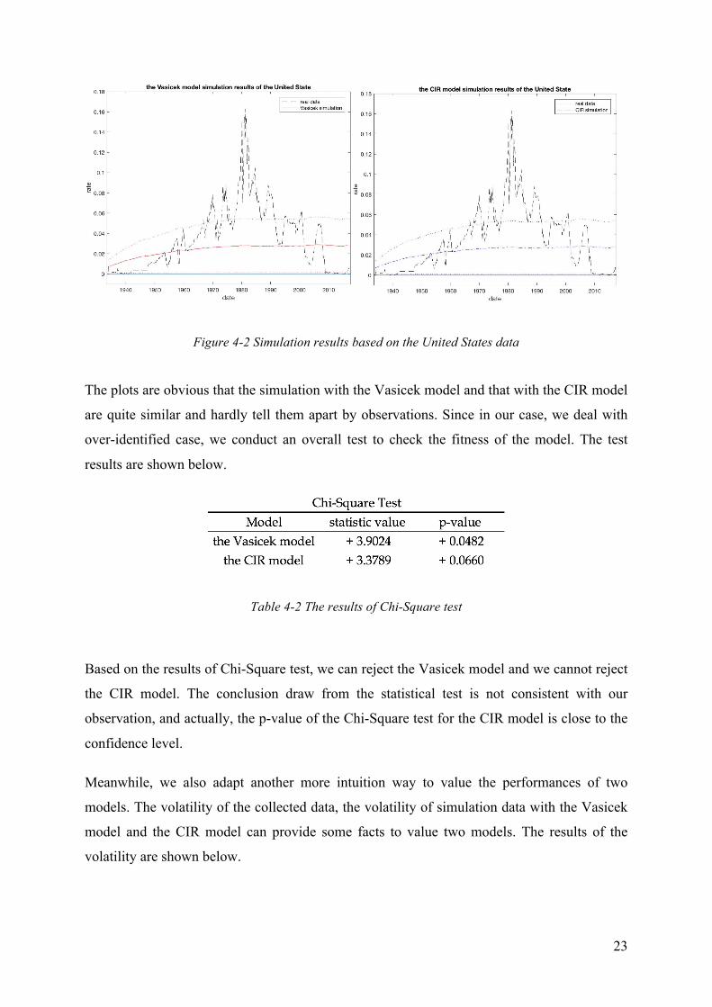
Figure 4-2 Simulation results based on the United States data

The plots are obvious that the simulation with the Vasicek model and that with the CIR model

are quite similar and hardly tell them apart by observations. Since in our case, we deal with

over-identified case, we conduct an overall test to check the fitness of the model. The test

results are shown below.

Table 4-2 The results of Chi-Square test

Based on the results of Chi-Square test, we can reject the Vasicek model and we cannot reject

the CIR model. The conclusion draw from the statistical test is not consistent with our

observation, and actually, the p-value of the Chi-Square test for the CIR model is close to the

confidence level.

Meanwhile, we also adapt another more intuition way to value the performances of two

models. The volatility of the collected data, the volatility of simulation data with the Vasicek

model and the CIR model can provide some facts to value two models. The results of the

volatility are shown below.

24

Table 4-3 Volatilities of the collected data, simulations within the Vasicek model and the CIR model

The volatility of the Vasicek model simulation and the volatility of CIR model simulation are

significantly close, it is a straightforward explanation for the similarity of the simulation plots.

Basically, with all the available data, the estimation results have highly similarity, hence the

similarity of the simulation results are understandable.

4.1.2 Empirical Result of United Kingdom

The result of estimated parameters we estimated with GMM are shown in the following table.

Table 4-4 The estimation results of the United Kingdom data

For the United Kingdom data case, the values of long-term mean for these two models are

similar, two models deliver similar and acceptable estimation. The following figure is the

volatility plot for both models.

25


Then, with the estimated parameters, we simulations and take average for the simulations and

the results of the simulation shown in the following figure.

Figure 4-4 Simulation results based on the United Kingdom data

We run overall test for both models, and the results of Chi-Square test are shown in the table

below.


26

Observed from the simulation plots, in the latest decade (from 2007 to 2017), the simulation

of the Vasicek model seems closer to the real data we collected than that of the CIR model,

the simulation of the Vasicek model delivered does not do better than the simulation of the

CIR model produced from 1980 to 2007. As the Chi-Square test shown, the Vasicek model is

rejected and the CIR model cannot be rejected. As we observed in the simulation plot, the

results of CIR simulation mimic the movement are similar to that of Vasicek model through

the whole time.

To value the Vasicek model and the CIR model in intuitional way, we also calculate the

volatilities (referring to standard deviations) of simulations with the Vasicek model,

simulations with the CIR model and the collected data. The results are shown in the following

table.


The volatilities of simulations within the Vasicek model and the CIR model are slightly lower

than the volatility of collected data. Observing the plots of simulation result, the volatility

results we get is consistent with observation.

4.1.3 Empirical Result of New Zealand

Using the GMM estimation method, we estimated the parameters (a, b and g), the results are

shown in the following table.

Table 4-7 The estimation results of New Zealand data

27

For New Zealand collected data, the long-term mean derived from the Vasicek model and the

CIR model are similar, hence two models deliver similar and acceptable estimation. The

volatility plots with estimated parameters are shown below.


Then same as before, we use the estimated parameters run simulation within 95% confidence

level and the simulation results are shown below.

Figure 4-6 Simulation results based on New Zealand data

The Vasicek model delivers a very similar simulation to the CIR model does, since the long-

term mean derived from these two models are both close to 0.04. It is not possible to conduct

28

reasoning about the goodness-of-fit from comparing the plots above alone. With an overall

test, it is reasonable to draw conclusion statistically, and the results are shown below.


Based on Chi-Square test results, both the Vasicek model and the CIR model cannot be

rejected. One possible reason we provide is that the interest rate before 1990 in New Zealand

are higher than the interest rate after 1990. We divide the timeline into two time periods, one

is before 1990 and the other is after 1990. Since for almost three decades, the interest rate

never grew back reaching the lowest interest rate level for the previous time period, the

interest rate in New Zealand does show obviously mean-reverting character as the models

expected in the last three decades (the last time period). Then, there is not a surprise that both

models show high goodness-to-fit and cannot be rejected statistically. From the Chi-Square

test, for relatively low volatility interest rate (refer to the last time period), the estimated

parameter g does not make big difference regardless g is equal to 0 or 0.5.

Also, we calculate the volatility to provide a more intuitive perspective.


From the table above, the volatilities calculated with simulation data is obviously lower than

the collected data. It also provides a more easily way to understand the higher goodness-of-fit

for the Vasicek model and the CIR model. For the last three decades and maybe in the future,

the interest rate will show less volatility but highly mean-reverting trend.

29

4.2 Robustness Check

Among all three counties interest rate data we collected, it is obvious that the data of the

United States is different. Since the long-term mean level is around 0.0286 (the average of the

long term means form two models estimated), and the normalized distribution of the data

shows the mean (µ) is around 0.045, then there is a large portion of the ineptest rate are higher

than the long-term mean. And the highest value of the interest rate is over 0.16, it leads us to

conduct a robustness check to test if the parameter estimated by the two models are affected.

We roughly separate the overall time period into three parts for further investigation. The

Bretton Woods System collapsed in 1971 and it started the so-called inflation woes. The after

the Jimmy Carter took the presidency of the United States in 1976, the inflation rate started

climb and the growth rate relatively smaller. Hence, we take the December 1976 as the start

point to take out the high interest rate time period. The Deregulation and the Reaganomics

boosted the U.S. economy for almost two decades from 1977, but the effects ends and the

government debt reached a new high point at early 1990s. We take December 1991 as the end

point since after 1990s, the 9/11 attack hit the United States economy hard and the interest

rates never increase back to the high level again. Hence, we separate the whole data into three

parts, which are from January 1934 to December 1976 (A), from January 1977 to December

1991 (B) and from January 1992 to December 2017 (C).

Following the pervious estimation steps, we estimate the parameters for each time period

separately.

For time period A, the estimation results are shown below, and the t-statistic in the

parentheses.

Table 4-10 The estimation results of the United States (A) data

30

As we can observe from the table above, the estimated long-term mean for both models are in

the same level but not close enough as the overall period estimation, hence, we plot the

estimated volatility in the following figure.


By observation, it is likely to think the estimation perhaps still similar as the overall time

period estimation. We also make simulation and plot the results, and the plots could bring us

closer to the conclusion.

Figure 4-2 Simulation results based on the United States (A) data

The plots are different from the previous simulation figures. For the Vasicek model, the

simulation growth much quicker than real data, but the CIR model delivers different direction

31

simulation. For two models, the 95% confidence level lines predicted each model include the

range of the real data. From the simulation plot, the CIR model provides more convincing

simulation.

We also did an overall test since this is still an over-identified case. The test results are shown

in the following table.


The overall test gives clearly answer, the Vasicek model is rejected and the CIR model cannot

be rejected. The p-value given by the CIR model estimation results, to some extent, could be

interpreted as that there are 99.67% real interest rate will occur in side the CIR model

confidence level.

Also, we still calculate the volatility and the results are in the following table.


From the information of the volatility, the rejection of the Vasicek model become more

reasonable, the volatility is too high to match the real data.

Then, we look into the highest interest rate time period (B) and the estimation results are

shown below.

32

Table 4-13 The estimation results of the United States (B) data

The estimation results are similar to the overall time period estimation results, hence we

expected the volatility plots and the simulation plots also show high similarity as the overall

related plots. The related plots are shown below.


Figure 4-4 Simulation results based on the United States (B) data

33

As we predicted, the plots are similar as that given by the overall time period estimation. For

statistically confirmation, we also run the Chi-Square test and the results are following.


The goodness-of-fit test shows we reject the Vasicek model and the CIR model. It is

reasonable, since even with 95% confidence level, there are still part of the highest values

falls out the boundary.

Table 4-15 Volatility of the collected data, simulations within the Vasicek model and the CIR model

We also compare the volatility as the table above and we observe that the volatilities of two

models are less than the half of the volatility of the real data. It is consistent with the Chi-

Square test conclusion that the models do not have enough volatility to mimic the movements

of the interest rate.

In the end, we look into the last time period time (C).

Table 4-16 The estimation results of the United States (C) data

34

The estimation results are obvious different with all other estimation results, since a in the

Vasicek model are estimated negative and b is estimated positive. The value of long-term

mean positive, so the estimation is possible. The reason for this situation is that within the

Vasicek model, the interest rate will decline in the long run. This result leads to a big

disagreement between the Vasicek model and the CIR model. We also plot the volatility of

interest rate and the simulation scenario.


Figure 4-6 Simulation results based on the United States (C) data

As we observe, the Vasicek model display the similar behaviours that occurred in the A time

period estimation.

35


The Chi-Square test shows that the Vasicek model is rejected and we cannot reject the CIR

model. The statistically results are similar to the A time period results.


The volatility information show that the Vasicek model over-estimates the volatility again,

like in the A time period.

Now, we treat these three separated time periods as one, for the Vasicek model, it is rejected

in each time period. As for the CIR model, it only fails when the volatility of the real data is

very large. The overall results are consistent when we treat them separately. Hence, the

Vasicek model and the CIR model both have some tolerance for extreme cases and the CIR

model performs better than the Vasicek model.

36

5 Conclusion

For all the simulation results and the test statistic result show that the results vary among the

countries. On the contrary, for the New Zealand data, it is more stable in the last two decades.

The United Kingdom data shown obvious mean-reverting before the credit crisis. For more

mean-reverting case, the parameter g needs to be higher than 0.5 based on previous researches

mentioned in section 3. The CIR model fit the real data better than the Vasicek model based

on the goodness-of-fit test we conducted. It is consistent with previous researched and calls

for more investigation we mentioned in section 2.

5.1 Practical Implications

The estimation we did in this paper, it shows that for real data with different counties, the

Vasicek model and the CIR model cannot mimic the movement well. Recall the research did

by Ait-Sahalia (1996b), the result will be different related to the range that the rate in. If the

rate does not deviate far from the mean, the dynamic pattern shows strong mean-reverting.

And if the rate deviates far from the mean, the parameters in the model need to be higher than

2. For our cases, all different simulation scenarios, only the CIR model for the United States

data delivers a simulation lines that reaches the long-term mean in the long run. Overall, the

CIR model suits three counties data better than Vasicek model. From these estimations we

get, the parameter g equals 0.5 is better than 0.

5.2 Improvement

Interest rates we used in our short-term interest rate are nominal interest rate. We did not

investigate into the dynamic real interest rate, although based on Fisher’s theory, real interest

rates are the sum of nominal interest rate and inflation. According to Sarte (1998), there were

some ‘higher-order’ parts into the equation make it more convincing, which related to

inflation. The dynamic pattern of real interest rate could be more unbiased than nominal

37

interest rate, but we think the nominal interest rate can be more intuitively show what’s going

on in the market. Meanwhile, we calculate the Unite States real interest rates and there are

many observations below zero, which is impossible for CIR model to simulate hence we do

not take real interest rates into our paper.

Meanwhile, we only discussed two basic models, the Vasicek model and the CIR model, and

as we mentioned in section 3, there are at least 6 more different one-factor short-term interest

rate model could be investigated. Within our estimation, the Vasicek model does not pass the

goodness-of-fit and be rejected by two of three counties real data. The plots of the simulation

show that for the United Kingdom and New Zealand, they both have much higher interest rate

and volatility level at the beginning of the observation time period than at the end of the

observation time period. These characteristics are not fully captured by the Vasicek model

and the CIR model. In the future, with more observations and estimated with more complex

models could deliver more satisfactory results.

38

References Ait-Sahalia, Y. (1996a). Nonparametric pricing of interest rate derivative securities,

Econometrica, vol. 64, no. 3, pp. 527–560

Ait-Sahalia, Y. (1996b). Testing continuous-time models of the spot interest rate, Review of

Financial Studies, vol. 9, no. 2, pp. 385-426

Ait-Sahalia, Y. (2002). Telling from discrete data whether the underlying continuous-time

model is a diffusion, The Journal of Finance, vol. 57, no. 5, pp. 2075-2112

Andersen, T. G., Chung, H. J., & Sørensen, B. E. (1999). Efficient method of moments

estimation of a stochastic volatility model: A Monte Carlo study, Journal of Econometrics,

vol. 91, no. 1, pp. 61-87.

Andrews, D. W. (1991). Heteroscedasticity and autocorrelation consistent covariance matrix

estimation, Econometrica: journal of the Econometric Society, vol. 59, no. 3, pp. 817-858

Arapis, M., & Gao, J. (2008). Nonparametric kernel estimation and testing in continuers-time

financial econometrics, Unpublished manuscript, Available Online: http://mpra.ub.uni-

muenchen.de/11974, [Accessed 9 December 2008]

Brockett, L. (2016). New Zealand cuts interest rates to record low: kiwi soars, Bloomberg

Markets Magazine, Available Online: https://www.bloomberg.com/news/articles/2016-08-

10/rbnz-cuts-key-rate-to-2-in-renewed-attempt-to-boost-inflation, [Accessed 08 March 2016]

Chan, K. C., Karolyi, G. A., Longstaff, F. A., & Sanders, A. B., (1992). An empirical

comparison of alternative models of the short-term interest rate, Journal of Finance, vol. 47,

no. 3, pp. 1209–27

Courtadon, G. (1982). The pricing of options on default-free bonds, Journal of Financial and

Quantitative Analysis, vol. 17, no. 1, pp. 75-100

39

Cox, J. C., Ingersoll Jr, J. E., & Ross, S. A. (1985). A theory of the term structure of interest

rate, Econometrica, vol. 53, no. 2, pp. 385-408

Elliott, L. (2014). Five key factors that will decide when Bank of England raises interest rates,

The Guardian, Available Online:

https://www.theguardian.com/business/2014/aug/17/interest-rates-go-up-five-points-bank-of-

england-decide, [Accessed 17 August 2014]

Florens-Zimrou, D. (1993). On estimating the diffusion coefficient from discrete

Observations, Journal of Applied Probability, vol. 30, no. 4, pp. 790-804

Hall, A. R. (2005). Generalized method of moments: advanced texts in econometrics, Oxford

University Press

Hansen, L.P. (1982). Large sample of generalized method of moments estimators,

Econometrica: journal of the Econometric Society, vol. 50, no. 4, pp. 1029-1054

Hansen, L.P., & Scheinkman, J.A. (1995). Back to the future: generating moment

implications for continuous-time Markov process, Econometrica, vol. 63, no. 4, pp. 767-804

James, J., & Webber, N. (2000). Interest Rate Modelling. Wiley-Blackwell Publishing Ltd.,

2000

Jiang, G. J., & Knight, J. L. (1997). A nonparametric approach to the estimation of diffusion

processes, with an application to a short-term interest rate model. Economic Theory, vol. 13,

no. 5, pp. 615-645

Khramov, M. V. (2013). Estimating parameters of the short-term real interest rate models.

International Monetary Fund, no. 13-212

Kladivko, K. (2007). The General Method of Moments (GMM) using MATLAB: The

practical guide based on the CKLS interest rate model. Department of Statistic and

Probability Calculus, University of Economics, Prague.

40

Nowman, K. B. (1997). Gaussian estimation of single-factor continuous time models of the

term structure of interest rates. Journal of Finance, vol. 52, no. 4, pp. 1965-1706

Sarte, P. D. G. (1998). Fisher’s equation and the inflation risk premium in a simple

endowment economy. Economic Quarterly, Federal Reserve Bank of Richmond, issue Fall,

pp. 53-72

Tang, C. Y., & Chen, S. X. (2009). Parameter estimation of bias correction for diffusion

processes, Journal of Econometrics, vol. 149, no. 1, pp. 65-81

Vasicek, O. (1976). An equilibrium characterization of the term structure. Journal of

Financial Economics, vol. 5, no. 2, pp. 177-188

Zeytun, S., & Gupta, A. (2007). A Comparative Study of the Vasicek and the CIR Model of

the Short Rate. Kaiserslautern, Germany: ITWM.

41

Appendix

Figure 5-1 The diffusion part for the United States Data

Figure 5-2 The diffusion part for the United Kingdom Data

Figure 5-3 The diffusion part for New Zealand Data

42

Figure 5-4 The diffusion part for the United States (A) Data

Figure 5-5 The diffusion part for the United States (B) Data

Figure 5-6 The diffusion part for the United States (C) Data

short-term interest rate models - lund...

Documents