Prepared in cooperation with the Interagency Special Status / Sensitive Species Program (ISSSSP). The ISSSSP is a cooperative program of the Pacific Northwest Regional Office of the U.S. Forest Service and Oregon/Washington State Office of the Bureau of Land Management

Short-Term Occupancy and Abundance Dynamics of the Oregon Spotted Frog (Rana pretiosa) Across Its Core Range

U.S. Department of the InteriorU.S. Geological Survey

Open-File Report 2014–1230

Cover: Oregon Spotted Frog, Rana pretiosa. Photograph by Brome McCreary, U.S. Geological Survey.

Short-Term Occupancy and Abundance Dynamics of the Oregon Spotted Frog (Rana pretiosa) Across Its Core Range

By Michael J. Adams, Christopher A. Pearl, Brome McCreary, and Stephanie K. Galvan

Prepared in cooperation with the Interagency Special Status / Sensitive Species Program (ISSSSP). The ISSSSP is a cooperative program of the Pacific Northwest Regional Office of the U.S. Forest Service and Oregon/Washington State Office of the Bureau of Land Management

Open-File Report 2014–1230

U.S. Department of the Interior U.S. Geological Survey

U.S. Department of the Interior SALLY JEWELL, Secretary

U.S. Geological Survey Suzette M. Kimball, Acting Director

U.S. Geological Survey, Reston, Virginia: 2014

For more information on the USGS—the Federal source for science about the Earth, its natural and living resources, natural hazards, and the environment—visit http://www.usgs.gov or call 1–888–ASK–USGS (1–888–275–8747)

For an overview of USGS information products, including maps, imagery, and publications, visit http://www.usgs.gov/pubprod

To order this and other USGS information products, visit http://store.usgs.gov

Any use of trade, firm, or product names is for descriptive purposes only and does not imply endorsement by the U.S. Government.

Although this information product, for the most part, is in the public domain, it also may contain copyrighted materials as noted in the text. Permission to reproduce copyrighted items must be secured from the copyright owner.

Suggested citation: Adams, M.J., Pearl, C.A., McCreary, B., and Galvan, S.K., 2014, Short-term occupancy and abundance dynamics of the Oregon spotted frog (Rana pretiosa) across its core range: U.S. Geological Survey Open-File Report 2014-1230, 10 p., http://dx.doi.org/10.3133/ofr20141230.

ISSN 2331-1258 (online)

iii

Contents Abstract ......................................................................................................................................................................... 1 Introduction .................................................................................................................................................................... 1 Methods ......................................................................................................................................................................... 2

Sampling Design ........................................................................................................................................................ 2 Field Surveys ............................................................................................................................................................. 2

Analysis ......................................................................................................................................................................... 4 Probability of Occupancy, Colonization, and Local Extinction .................................................................................... 4 Abundance ................................................................................................................................................................. 5

Results ........................................................................................................................................................................... 5 Discussion ..................................................................................................................................................................... 6 Summary ....................................................................................................................................................................... 7 Acknowledgments ......................................................................................................................................................... 7 References Cited ........................................................................................................................................................... 8 Appendix A. Site Names, Cluster Names, Frame Assignments, and Coordinates of Survey Sites ............................... 9

Figure Figure 1. Map showing locations surveyed for Oregon spotted frogs (Rana pretiosa) in the Deschutes and Klamath Basins, Oregon, 2010–13. ........................................................................................................................ 3

Table Table 1. Multi-season occupancy models describing the probability that a site was occupied by breeding stages of Oregon spotted frog (Rana pretiosa), Deschutes and Klamath Basins, Oregon, 2010–13 ............................................ 6

iv

Conversion Factors and Datum Conversion Factors SI to Inch/Pound

Multiply By To obtain

Length meter (m) 3.281 foot (ft)

kilometer (km) 0.6214 mile (mi)

meter (m) 1.094 yard (yd)

Datum Horizontal coordinate information is referenced to the North American Datum of 1983 (NAD 83).

1

Short-Term Occupancy and Abundance Dynamics of the Oregon Spotted Frog (Rana pretiosa) Across Its Core Range

By Michael J. Adams, Christopher A. Pearl, Brome McCreary, and Stephanie K. Galvan

Abstract The Oregon spotted frog (Rana pretiosa) occupies only a fraction of its original range and is

listed as Threatened under the Endangered Species Act. We surveyed 93 sites in a rotating frame design (2010–13) in the Klamath and Deschutes Basins, Oregon, which encompass most of the species’ core extant range. Oregon spotted frogs are declining in abundance and probability of site occupancy. We did not find an association between the probability that Oregon spotted frogs disappear from a site (local extinction) and any of the variables hypothesized to affect Oregon spotted frog occupancy. This 4-year study provides baseline data, but the 4-year period was too short to draw firm conclusions. Further study is essential to understand how habitat changes and management practices relate to the status and trends of this species.

Introduction The Oregon spotted frog (Rana pretiosa) is listed as Threatened under the Endangered Species

Act (U.S. Fish and Wildlife Service, 2014) and Vulnerable on the Red List of Threatened Species (International Union for Conservation of Nature, 2013). Our understanding that this species has declined is based on its absence from portions of its range (Pearl and Hayes, 2005), but there is a lack of reliable information on trends in abundance or on the probability of site occupancy. For example, there is currently no information to suggest whether Oregon spotted frogs are still disappearing from occupied sites, if they are colonizing new sites, or if their abundance on average is increasing or decreasing. This information is essential to a basic understanding of the status and trends of this species.

The current core extant range of the Oregon spotted frog is from southern British Columbia to southern Oregon. Distribution is disjunct in the northern part of the range and the species is thought to be absent from the Willamette Valley (Jones and others, 2005). The core extant range is mostly in the Deschutes and Klamath Basins of Oregon, with a few additional sites occupied near the headwaters of the Willamette and McKenzie Rivers just west of the divide from the Deschutes Basin drainage (Pearl and others, 2009) and in the northern Oregon Cascades. Hypothesized threats to Oregon spotted frog persistence are invasive species, disease, habitat changes, population isolation, and climate change. Habitat changes may result from changes in beaver (Castor canadensis) activity, management practices that enable encroachment of woody vegetation on historically open wetlands, fire and fuels management, or hydrological manipulations (Pearl and Hayes, 2005). We emphasize that there is little empirical support for any of these hypotheses and, although the species is clearly absent from portions of its historical range, there is little information on current trends.

2

We are addressing three objectives for the core extant range of the Oregon spotted frog: (1) to estimate site-level probability of occupancy, colonization, and extinction rates; (2) to estimate the overall trend in abundance; and (3) to determine the correlation of site characteristics related to habitat succession and disturbance with the probability of local extinction. These objectives are fundamental to understanding the status and trends of Oregon spotted frogs, but will take many years of data to convincingly assess. Here, we report an analysis of the first 4 years of data from this effort.

Methods Sampling Design

We used a 4-year rotating frame design to sample lentic habitats in the core range of the Oregon spotted frog (fig. 1). Lentic habitats, hereafter “sites,” were ponds, lakes, wetlands, oxbows, and sloughs. The core range was defined as all known occupied sites in Oregon at the initiation of this study plus most known historical sites plus lentic habitats in close proximity to current and historical sites (appendix 1). Exceptions were (1) the Willamette Valley where Oregon spotted frogs have not been seen in decades, (2) nine sites where intensive population monitoring was already occurring, and (3) three sites that were too large to survey. Our rotating frame design consisted of one fixed frame sampled each year and four rotating frames sampled once each during the 4-year study (appendix 1; fig. 1). This definition of the sampling frame resulted in 93 sites. All 93 sites were grouped into spatial clusters for ease of sampling. Clusters were all randomly assigned to frames. Each site was surveyed for the presence of Oregon spotted frog one to three times in any year that it was part of the sample (appendix 1). Survey frequency was randomly assigned to sites. Our aim was to survey 50 percent of sites two times and 25 percent of sites three times. When possible, additional surveys were completed in a random order.

Field Surveys A survey consisted of two technicians searching all portions of a site with water less than 1 m

deep for Oregon spotted frogs. Crews recorded air temperature at start, midway, and conclusion of surveys. Technicians searched by slowly walking the perimeter of the site, visually searching for amphibians of any stage, and completing a minimum of five dip-net sweeps at least 10 m apart in microhabitats that could conceal amphibians. Surveys were conducted between 08:00 and 20:00 hours from early June to mid-August from 2010 through 2013.

Habitat variables were recorded during each survey. Between 5 and 15 plots were spread evenly around the perimeter of each site and were used to assess shading and vegetation. “Shade” was the average height (in degrees) of vegetation or the horizon affecting the plot. It was measured using a clinometer aimed at the compass bearings of 170, 180, and 190 degrees. “Veg” was the average percentage of a transect that had visible emergent, submergent, or floating vegetation. Transects ran perpendicular to shore from each plot to the other side of the site.

“Beaver” was coded as “1” if a site was influenced by beaver activities and was otherwise coded “0.” We considered a site beaver-influenced if any beaver sign was recorded, including old and inactive dams. We used “deep” = 1 if the maximum depth of a site appeared greater than 2 m; otherwise “deep” = 0. We obtained elevation (“elev”) from a Digital Elevation Model. We classified “basin” for each site based on whether it was located in the Deschutes or Klamath hydrographic basins. We combined the three Willamette Basin sites with the Deschutes Basin sites because they were few and were near the divide between basins.

3

Figure 1. Map showing locations surveyed for Oregon spotted frogs (Rana pretiosa) in the Deschutes and Klamath Basins, Oregon, 2010–13.

4

Analysis Probability of Occupancy, Colonization, and Local Extinction

For this analysis, occupied sites were those that had eggs, larvae, or metamorphic stages of Oregon spotted frogs. We used the function “colext” from the package “unmarked” (v. 0.10-2) in R (v. 3.0.2) to estimate site-level probabilities for initial occupancy, colonization, and local extinction while accounting for the fact that surveys will sometimes fail to detect Oregon spotted frogs when they are present and that the probability of detecting frogs that are present (p) is likely to vary (Fiske and Chandler, 2011; R Core Team, 2013). The function “colext” fits the multi-season occupancy model of MacKenzie and others (2003). We used this model to investigate how the probability of local extinction (ε) related to site characteristics and to derive estimates of ψ, the probability that a site is occupied. Because we only had 4 years of data and because those data included rotating frames, we expected that it would be difficult to estimate the transition probabilities. We therefore used a simplifying assumption that colonization (γ) was constant across years and sites.

We used the global model: ψ(veg), ε(veg,shade,beaver,basin,elev,deep), γ(.), p(day,Atemp,year,veg,beaver,basin,elev,shade,deep)

We included ordinal date of surveys (day) because changes in behavior and abundance over the season might affect p. “Atemp” was the average of the air temperatures measured at the beginning and end of a survey. It was included because it is known to affect frog activity so might affect p. The covariate “year” was included because we were interested in the trend in occupancy over years and p might vary over years with changes in crew or habitat changes. All others were included so that variation in p would not bias estimates of their effects on ε. We investigated quadratic effects on p for “day” and “Atemp,” but neither convincingly improved the model (ΔAIC less than 2; AIC=Akaike’s Information Criteria). We removed p (year) for subsequent analysis because doing so decreased AIC by 4.8. We retained all other covariates of p because removing them individually did not convincingly improve the model.

We included “veg” as a covariate of ψ because emergent vegetation has often been associated with Oregon spotted frogs and other anuran occurrence and abundance (Pearl and others, 2005; Adams and others, 2011).

To estimate initial occupancy (ψ1), γ, and ε, we fit a colext model with the following covariates of each parameter:

ψ1(veg), ε(),γ(), p(day, Atemp, veg, beaver, basin, elev, shade, deep) To compare the effects of site characteristics on ε, we fit the following variations on the ε

portion of the model leaving the ψ, γ, and p portions as shown above: ε(veg), ε(beaver), ε(basin), ε(elev), ε(shade), ε(deep), ε(.) We ran the occupancy analysis with data from all frames and repeated the analysis with data

from the fixed frame only to determine if the lack of multiple years of data for the rotating frames could be biasing results. Because the fixed frame only includes 17 sites, we used a model for p that did not include basin, elev, shade, and deep. These variables had little effect on AIC when all data were included and we needed to simplify the fixed-frame model to accommodate the small number of sites.

5

Abundance We used the function “pcountOpen” from the package “unmarked” in R to estimate trends in

abundance of post-metamorphic stages of Oregon spotted frogs (that is, juveniles, subadults, and adults). This function fits an N-mixture model that accounts for the fact that the number of animals counted during a field survey is less than the number of animals present and that the difference is both variable and unobserved (Royle, 2004; Dail and Madsen, 2011). We used the negative binomial error structure because it fit better than the Poisson or zero-inflated Poisson structures based on AIC. We used the “trend” parameterization of the model, which estimated the trend in abundance instead of survival and compared the best model with the “no-trend” parameterization to assess evidence for a trend. In the trend model, the parameter γ is used as the finite rate of increase, which is often referred to as λ in the ecological literature and that is how we refer to it in the Results section below. We used K=675 as an estimate of maximum population size, which was enough to stabilize parameter estimates. This model evaluates every population size up to K at every site so becomes very slow with higher values of K. For this reason, we removed one site that had an abnormally high count during one visit. Attempts to analyze the full dataset including that site were unsuccessful.

The abundance models took days of computer time to run, so we sought the simplest reasonable parameterization. To estimate the trend in abundance we fit:

N(veg), λ(), p(day, day2, Atemp, Atemp2, veg, year)

Results The probability of detecting Oregon spotted frogs at a site when the species was present varied

among years with mean of the annual estimates ranging from 0.38 (SE=0.078) to 0.72 (SE=0.087). This variation was best explained by the timing of surveys and air temperature. A model with p(day+temp) was supported over p(year), and adding year to p(day+temp) did not improve the model based on AICc (Akaike’s Information Criteria for small sample size).

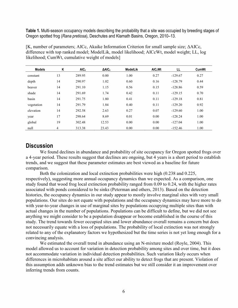
There was little differentiation in the support for various models of extinction probability with only the null model, the global model, and a model with separate estimates of extinction probability for each year being clearly dismissed (table 1). The constant model ε(.) was marginally best and was used for parameter estimation.

The overall estimate of ψ decreased from 0.69 (SE=0.085) to 0.53 (SE=0.093) in 4 years. The probability that a site unoccupied 1 year was colonized the next year was 0.238 (SE=0.11; CI=0.09–0.50). The probability that a site occupied 1 year became unoccupied (locally extinct) the next year was 0.225 (SE=0.080; CI=0.11–0.42). The naïve occupancy each year sequentially was 0.31, 0.39, 0.43, 0.35.

When only the data from the fixed frame were used, the estimate of ψ decreased from 0.66 (SE=0.156) in the first year to 0.37 (SE=0.130) in the fourth year. The naïve occupancy for the fixed frame each year sequentially was 0.41, 0.47, 0.52, 0.29.

Mean weighted counts of adults at the fixed frame sites were 14.4, 5.3, 4.9, and 6.4 annually from 2010 to 2013. Using data from all frames, the open abundance model compensated for variation in capture probability among years and visits and suggests a decrease in the number of adult and juvenile Oregon spotted frogs with an instantaneous growth rate of λ=0.80 (SE=0.051; CI=0.70–0.90). The trend model was strongly favored over the no trend model (ΔAICc=124).

6

Table 1. Multi-season occupancy models describing the probability that a site was occupied by breeding stages of Oregon spotted frog (Rana pretiosa), Deschutes and Klamath Basins, Oregon, 2010–13. [K, number of parameters; AICc, Akaike Information Criterion for small sample size; ΔAICc, difference with top ranked model; ModelLik, model likelihood; AICcWt, model weight; LL, log likelihood; CumWt, cumulative weight of models]

Models K AICc ΔAICc ModelLik AICcWt LL CumWt constant 13 289.95 0.00 1.00 0.27 -129.67 0.27

depth 14 290.97 1.02 0.60 0.16 -128.79 0.44

beaver 14 291.10 1.15 0.56 0.15 -128.86 0.59

shade 14 291.69 1.74 0.42 0.11 -129.15 0.70

basin 14 291.75 1.80 0.41 0.11 -129.18 0.81

vegetation 14 291.79 1.84 0.40 0.11 -129.20 0.92

elevation 14 292.58 2.63 0.27 0.07 -129.60 1.00

year 17 298.64 8.69 0.01 0.00 -128.24 1.00

global 19 302.48 12.53 0.00 0.00 -127.04 1.00

null 4 313.38 23.43 0.00 0.00 -152.46 1.00

Discussion

We found declines in abundance and probability of site occupancy for Oregon spotted frogs over a 4-year period. These results suggest that declines are ongoing, but 4 years is a short period to establish trends, and we suggest that these parameter estimates are best viewed as a baseline for future comparison.

Both the colonization and local extinction probabilities were high (0.238 and 0.225, respectively), suggesting more annual occupancy dynamics than we expected. As a comparison, one study found that wood frog local extinction probability ranged from 0.09 to 0.24, with the higher rates associated with ponds considered to be sinks (Peterman and others, 2013). Based on the detection histories, the occupancy dynamics in our study appear to mostly involve marginal sites with very small populations. Our sites do not equate with populations and the occupancy dynamics may have more to do with year-to-year changes in use of marginal sites by populations occupying multiple sites than with actual changes in the number of populations. Populations can be difficult to define, but we did not see anything we might consider to be a population disappear or become established in the course of this study. The trend towards fewer occupied sites and lower abundance overall remains a concern but does not necessarily equate with a loss of populations. The probability of local extinction was not strongly related to any of the explanatory factors we hypothesized but the time series is not yet long enough for a convincing analysis.

We estimated the overall trend in abundance using an N-mixture model (Royle, 2004). This model allowed us to account for variation in detection probability among sites and over time, but it does not accommodate variation in individual detection probabilities. Such variation likely occurs when differences in microhabitats around a site affect our ability to detect frogs that are present. Violation of this assumption adds unknown bias to the trend estimates but we still consider it an improvement over inferring trends from counts.

7

The use of a rotating frame is problematic in a monitoring study (MacKenzie and others, 2006). We used this design rather than monitoring a fixed random subset of sites because the funding agencies requested that all sites within the range of inference be visited. A rotating frame design adds year-to-year variation associated with the different frames surveyed in a given year. Although most of the information for estimating transition probabilities comes from the fixed frame, these estimates must be reconciled in the likelihood with the variation in ψ indicated by both the fixed frame and the rotating frames. This requires an assumption that the transition probabilities are the same for each frame. This assumption is theoretically plausible in our study because we randomly assigned clusters of sites to frames. The magnitude of decline was greater for the fixed frame than for the full data, which adds credibility to the conclusion that Oregon spotted frogs continue to decline in our study area.

Our detection probabilities were somewhat low, with an average of 0.62 (SE=0.056). This leads to a loss of precision and potentially biases parameter estimates (McKann and others, 2013). Future work might improve p with more repeat surveys or constraints on when sampling occurs. For example, a minimum air temperature for field surveys could limit observations under marginal conditions for detecting species that are present.

Although there is much information suggesting unprecedented declines in amphibians as a group, there remains little quantitative data on individual species trends (Adams and others, 2013). The U.S. Fish and Wildlife Service is required to evaluate the status of candidate, threatened, and endangered species. Obtaining reliable information on status and trends requires studies that: (1) have broad statistical inference to an area of interest either by probabilistic or, as in our study, by complete sampling; and (2) are designed to accommodate imperfect detection. Our study provides quantitative information that Oregon spotted frogs may be continuing to decline in Oregon. The 4-year period of this study is too short to draw firm conclusions about current trends but lays a foundation for a more rigorous future assessment of trends and options to manage habitats to the benefit of the species.

Summary The Oregon spotted frog (Rana pretiosa) is considered Threatened under the Endangered

Species Act. Over the past 4 years, we used a rotating frame design to monitor Oregon spotted frogs in their core extant range located in the Klamath and Deschutes Basins, Oregon. We assessed occupancy, colonization, and extinction rates, overall trends in abundance, and determined the correlation between habitat succession and disturbance variables with the probability of local extinction. Although our analysis indicates that the Oregon spotted frog is experiencing declines in abundance and probability of site occupancy, we acknowledge that 4 years is brief time over which to establish convincing trends.

Acknowledgments This study was made possible in part by funding from the Interagency Special Status / Sensitive

Species Program (ISSSSP). The ISSSSP is a cooperative program of the Pacific Northwest Regional Office of the U.S. Forest Service and Oregon/Washington State offices of the Bureau of Land Management. Additional funding was provided by the U.S. Geological Survey’s Amphibian Research and Monitoring Initiative (ARMI). We thank Kelli Van Norman (Bureau of Land Management) for continued support of our work. We also thank our public and private cooperators, among them Klamath Marsh National Wildlife Refuge, the Deschutes, Willamette, and Fremont-Winema National Forests, the Prineville Resource Area (BLM), and Sunriver Nature Center. This is product 489 of the Amphibian Research and Monitoring Initiative.

8

References Cited Adams, M.J., Miller, D.A.W., Muths, E., Corn, P.S., Grant, E.H.C., Bailey, L.L., Fellers, G.M., Fisher,

R.N., Sadinski, W.J., Waddle, H., and Walls, S.C., 2013, Trends in amphibian occupancy in the United States: PLoS One, v. 8, e64347.

Adams, M.J., Pearl, C.A., Galvan, S., and McCreary, B., 2011, Non-native species impacts on pond occupancy by an anuran: Journal of Wildlife Management, v. 75, p. 30–35.

Dail, D., and Madsen, L., 2011, Models for estimating abundance from repeated counts of an open metapopulation: Biometrics, v. 67, p. 577–587.

Fiske, I., and Chandler, R.B., 2011, Unmarked—An R package for fitting hierarchical models of wildlife occurrence and abundance: Journal of Statistical Software, v. 43, p. 1–23.

International Union for Conservation of Nature, 2013, The IUCN Red List of Threatened Species: International Union for Conservation of Nature, v. 2014.2, accessed August 6, 2014, at http://www.iucnredlist.org.

Jones, L.L.C., Leonard, W.P., and Olson, D., 2005, Amphibians of the Pacific Northwest: Seattle, Washington, Seattle Audubon Society, 227 p.

MacKenzie, D.I., Nichols, J.D., Hines, J.E., Knutson, M.G., and Franklin, A.B., 2003, Estimating site occupancy, colonization, and local extinction when a species is detected imperfectly: Ecology, v. 84, p. 2,200–2,207.

MacKenzie, D.I., Nichols, J.D., Royle, J.A., Pollock, K.H., Bailey, L.L., and Hines, J.E., 2006, Occupancy estimation and modeling: Boston, Massachusets, Academic Press, 344 p.

McKann, P.C., Gray, B.R., and Thogmartin, W.E., 2013, Small sample bias in dynamic occupancy models: The Journal of Wildlife Management, v. 77, p. 172–180.

Pearl, C.A., Adams, M.J., and Leuthold, N., 2009, Breeding habitat and local population size of the Oregon spotted frog (Rana pretiosa) in Oregon, USA: Northwestern Naturalist, v. 90, p. 136–147.

Pearl, C.A., Bowerman, J., and Knight, D., 2005, Feeding behavior and aquatic habitat use by Oregon spotted frogs (Rana pretiosa) in central Oregon: Northwestern Naturalist, v. 86, p. 36–38.

Pearl, C.A., and Hayes, M.P., 2005, Rana pretiosa, Oregon spotted frog, in Lannoo, M.J., ed., Amphibian declines—The conservation status of United States species: Oakland, University of California Press, p. 577–580.

Peterman, W.E., Rittenhouse, T.A.G., Earl, J.E., and Semlitsch, R.D., 2013, Demographic network and multi-season occupancy modeling on Rana sylvatica reveal spatial and temporal patterns of population connectivity and persistence: Landscape Ecology, v. 28, p. 1,601–1,613.

R Core Team, 2013, R—A language and environment for statistical computing: Vienna, Austria, R Foundation for Statistical Computing, accessed August 6, 2014, at http://www.R-project.org/.

Royle, J.A., 2004, N-mixture models for estimating population size from spatially replicated counts: Biometrics, v. 60, p. 108–115.

U.S. Fish and Wildlife Service, 2014, 50 CFR Part 17—Endangered and threatened wildife and plants: U.S. Fish and Wildlife Service, p. 51,657–51,710, accessed August 29, 2014, at http://www.gpo.gov/fdsys/pkg/FR-2014-08-29/pdf/2014-20059.pdf.

9

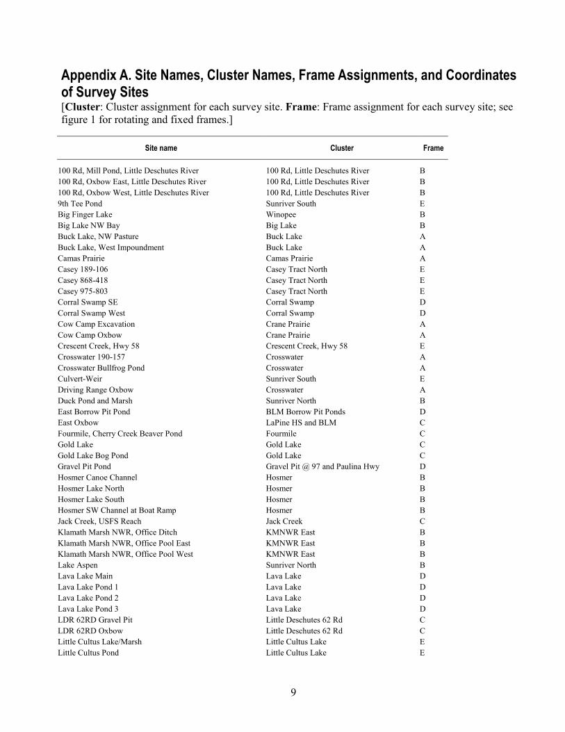
Appendix A. Site Names, Cluster Names, Frame Assignments, and Coordinates of Survey Sites [Cluster: Cluster assignment for each survey site. Frame: Frame assignment for each survey site; see figure 1 for rotating and fixed frames.]

Site name Cluster Frame

100 Rd, Mill Pond, Little Deschutes River 100 Rd, Little Deschutes River B 100 Rd, Oxbow East, Little Deschutes River 100 Rd, Little Deschutes River B 100 Rd, Oxbow West, Little Deschutes River 100 Rd, Little Deschutes River B 9th Tee Pond Sunriver South E Big Finger Lake Winopee B Big Lake NW Bay Big Lake B Buck Lake, NW Pasture Buck Lake A Buck Lake, West Impoundment Buck Lake A Camas Prairie Camas Prairie A Casey 189-106 Casey Tract North E Casey 868-418 Casey Tract North E Casey 975-803 Casey Tract North E Corral Swamp SE Corral Swamp D Corral Swamp West Corral Swamp D Cow Camp Excavation Crane Prairie A Cow Camp Oxbow Crane Prairie A Crescent Creek, Hwy 58 Crescent Creek, Hwy 58 E Crosswater 190-157 Crosswater A Crosswater Bullfrog Pond Crosswater A Culvert-Weir Sunriver South E Driving Range Oxbow Crosswater A Duck Pond and Marsh Sunriver North B East Borrow Pit Pond BLM Borrow Pit Ponds D East Oxbow LaPine HS and BLM C Fourmile, Cherry Creek Beaver Pond Fourmile C Gold Lake Gold Lake C Gold Lake Bog Pond Gold Lake C Gravel Pit Pond Gravel Pit @ 97 and Paulina Hwy D Hosmer Canoe Channel Hosmer B Hosmer Lake North Hosmer B Hosmer Lake South Hosmer B Hosmer SW Channel at Boat Ramp Hosmer B Jack Creek, USFS Reach Jack Creek C Klamath Marsh NWR, Office Ditch KMNWR East B Klamath Marsh NWR, Office Pool East KMNWR East B Klamath Marsh NWR, Office Pool West KMNWR East B Lake Aspen Sunriver North B Lava Lake Main Lava Lake D Lava Lake Pond 1 Lava Lake D Lava Lake Pond 2 Lava Lake D Lava Lake Pond 3 Lava Lake D LDR 62RD Gravel Pit Little Deschutes 62 Rd C LDR 62RD Oxbow Little Deschutes 62 Rd C Little Cultus Lake/Marsh Little Cultus Lake E Little Cultus Pond Little Cultus Lake E

10

Site name Cluster Frame

Little Lava Lake Little Lava Lake D Little Lava NW Little Lava Lake D Little Lava SE Little Lava Lake D Long Prairie Long Prairie B Long Prairie Marsh LaPine HS and BLM C Loosely Spring Pond KMNWR D Lower Blue Pool, Main Lower Blue Pool D Lower Blue Pool, North Shelf Pond Lower Blue Pool D Lower Blue Pool, South Shelf Pond Lower Blue Pool D Mowich Log Pond Mowich on Little Deschutes River E Muskrat Lake Muskrat Lake A Nature Center Pond Sunriver North B North Driving Range Pond Crosswater A Odell Creek NE fen Odell Creek E Odell Creek SW fen Odell Creek E Parsnip Lakes, Lower Parsnip Lakes C Parsnip Lakes, Main Beaver Pond Parsnip Lakes C Parsnip Mid Parsnip Lakes C Parsnip Temp pond above Main Beaver Pond Parsnip Lakes C Pit East of Rt 46 Crane Prairie A Pit West of Rt 46 Crane Prairie A Pond SE of Crane Prairie Reservoir Crane Prairie A Ranger Creek Davis Lake C Rear Driving Range Pond Crosswater A Sevenmile Creek, Lower Beaver Pond Sevenmile Creek E Sevenmile Creek, Middle Beaver Pond Sevenmile Creek E Sevenmile Creek, Upper Beaver Pond Sevenmile Creek E Snowshoe Lake Winopee B Thousand 016-554 Thousand Trails D Thousand 617-004 Thousand Trails D Thousand 657-347 Thousand Trails D Thousand 725-178 Thousand Trails D Thousand 770-245 Thousand Trails D Thousand 794-542 Thousand Trails D Thousand 927-566 Thousand Trails D Tunnell Creek, 2nd Beaver Pond Buck Lake A Tunnell Creek, Upper Beaver Pond Buck Lake A Twin Rivers Pond Crosswater A Upper Blue Pool Upper Blue Pool E Upper Oxbow on Little Deschutes River Mowich on Little Deschutes River E Upper Williamson River USFS Upper Williamson B Vista-Lodge Sunriver South E West Borrow Pit Pond BLM Borrow Pit Ponds D Wickiup Pit Wickiup C Winopee 366-425 Winopee B Winopee 858-175 Winopee B Winopee 947-462 Winopee B Winopee Lake Winopee B

Publishing support provided by the U.S. Geological SurveyPublishing Network, Tacoma Publishing Service Center

For more information concerning the research in this report, contact the Director, Forest and Rangeland Ecosystem Science Center

U.S. Geological Survey 777 NW 9th St., Suite 400 Corvallis, Oregon 97330 http://fresc.usgs.gov/

Adams and others—

Short-Term O

ccupancy and Abundance D

ynamics of the O

regon Spotted Frog (Rana pretiosa) Across Its Core Range—

Open-File Report 2014–1230

ISSN 2331-1258 (online)http://dx.doi.org/10.3133/ofr20141230