short-term scheduling lecture -...
TRANSCRIPT

SHORT-TERM SCHEDULING
CARLOS A. MENDEZ
Instituto de Desarrollo Tecnológico para la Industria Química (INTEC)Universidad Nacional de Litoral (UNL) – CONICET
Güemes 3450, 3000 Santa Fe, [email protected]
PASI 2008 PASI 2008 -- Mar del Plata, ArgentinaMar del Plata, Argentina

PASI 2008 PASI 2008 -- Mar del Plata, ArgentinaMar del Plata, Argentina
OUTLINE
PROBLEM STATEMENT
MAJOR FEATURES AND CHALLENGES
SOLUTION METHODS
MILP-BASED MODELS
EXAMPLES AND COMPUTATIONAL ISSUES
INDUSTRIAL-SCALE PROBLEMS
PASI 2008 PASI 2008 -- Mar del Plata, ArgentinaMar del Plata, Argentina
LITERATURE. REVIEW PAPERS
Floudas, C A., & Lin, X. (2004). Continuous-time versus discrete-time approaches for schedulingof chemical processes: A review. Computers and Chemical Engineering, 28, 2109–2129.
Pinto, J.M., & Grossmann, I.E. (1998). Assignments and sequencing models of the scheduling ofprocess systems. Annals of Operations Research, 81, 433–466.
Pekny, J.F., & Reklaitis, G.V. (1998). Towards the convergence of theory and practice: A technologyguide for scheduling/planning methodology. In Proceedings of the third international conference on foundations ofcomputer-aided process operations (pp. 91–111).
Kallrath, J. (2002). Planning and scheduling in the process industry. OR Spectrum, 24, 219–250.
Shah, N. (1998). Single and multisite planning and scheduling: Current status and future challenges. In Proceedings of the third international conference on foundations of computer-aided process operations (pp. 75–90).
Méndez, C.A., Cerdá, J., Harjunkoski, I., Grossmann, I.E. & Fahl, M. (2006). State-of-the-art review of optimization methods for short-term scheduling of batch processes. Computers and Chemical Engineering, 30, 6, 913 – 946,

PASI 2008 PASI 2008 -- Mar del Plata, ArgentinaMar del Plata, Argentina
TRADITIONAL "BIG PICTURE"
Plant Level: Multilevel/Hierarchical Decisions
Planning
Scheduling
Control
Economics
Feasibility Delivery
Dynamic Performance
months, years
days, weeks
secs, mins
Information systemsOptimization-based computer tools
Allocation of limited resources over time to perform a collection
of tasks
“Decision-making process with the goal of optimizing one or more objectives”

PASI 2008 PASI 2008 -- Mar del Plata, ArgentinaMar del Plata, Argentina
SHORT-TERM SCHEDULING
Scheduler
Schedule
Plant configurationRecipe dataDemands
Production SchedulingProduction SchedulingDetailed plant production scheduling

PASI 2008 PASI 2008 -- Mar del Plata, ArgentinaMar del Plata, Argentina
WhatWhat
HowHow
WhereWhere
WhenWhen
Batches or campaigns to be processed
resource allocation: steam, electricity, raw materials, manpower
unit allocation
Timing of manufacturing operations
DECISION-MAKING PROCESS
MAIN CHALLENGESHigh combinatorial complexity
Many problem features to be simultaneously considered
Time restrictions

PASI 2008 PASI 2008 -- Mar del Plata, ArgentinaMar del Plata, Argentina
profit = 2805
Heater
Reactor 1
Reactor 2
Still
HeatingReaction 3
Reaction 1
Reaction 2
Separation
EQUIPMENT-HEATER
- 2 REACTORS-STILL
DECISIONSLot-sizing
Allocation
Sequencing
Timing
ILLUSTRATIVE EXAMPLE
BATCH TASKS-HEATING
- 3 REACTIONS- SEPARATION
GOALMAXIMIZE PROFIT
STN-REPRESENTATION
PASI 2008 PASI 2008 -- Mar del Plata, ArgentinaMar del Plata, Argentina
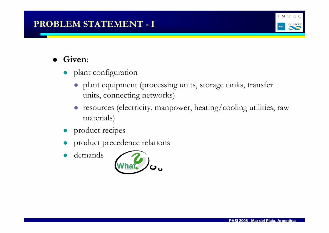
Given:plant configuration
plant equipment (processing units, storage tanks, transfer units, connecting networks)resources (electricity, manpower, heating/cooling utilities, rawmaterials)
product recipesproduct precedence relationsdemands
WhatWhat
PROBLEM STATEMENT - I
PASI 2008 PASI 2008 -- Mar del Plata, ArgentinaMar del Plata, Argentina
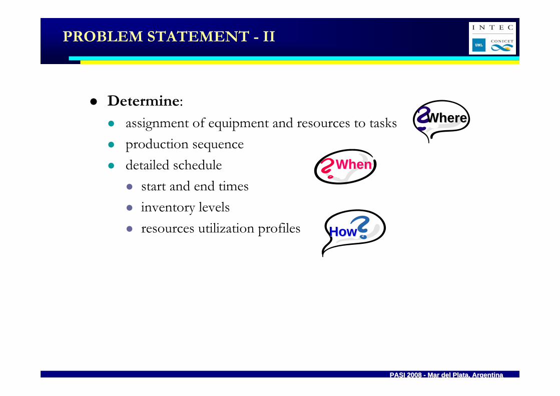
Determine:assignment of equipment and resources to tasksproduction sequencedetailed schedule
start and end timesinventory levelsresources utilization profiles HowHow
WhereWhere
WhenWhen
PROBLEM STATEMENT - II

PASI 2008 PASI 2008 -- Mar del Plata, ArgentinaMar del Plata, Argentina
To optimize one or more objectives:time required to complete all tasks (makespan)number of tasks completed after their due datesplant throughputcustomer satisfaction profitcosts
PROBLEM STATEMENT - III

PASI 2008 PASI 2008 -- Mar del Plata, ArgentinaMar del Plata, Argentina
WhatWhat
HowHow
WhenWhen
WhereWhere
II Execution
IDecision making
Predictive schedule
INFEASIBLE SCHEDULE
dynamic & uncertaindynamic & uncertainenvironmentenvironment
Unexpected events
ambiguousoutdatedincomplete
Data
SCHEDULING & RE-SCHEDULING
RESCHEDULINGRESCHEDULING““Efficient resource Efficient resource
relocationrelocation””

PASI 2008 PASI 2008 -- Mar del Plata, ArgentinaMar del Plata, Argentina
BATCH SCHEDULING FEATURES
(1) Process topology Sequential Network
(arbitrary) Single stage Multiple stages
Single Parallel Multiproduct Multipurpose unit units (Flow-shop) (Job-shop)
(2) Equipment assignment Fixed Variable
(3) Equipment connectivity Partial Full
(restricted)
(4) Inventory storage policies Unlimited Non-Intermediate Finite Zero
Intermediate Storage (NIS) Intermediate Wait (ZW) Storage (UIS) Storage (FIS)
Dedicated Shared
storage units storage units
(5) Material transfer Instantaneous Time-consuming (neglected)
No-resources Pipes Vessels (Pipeless)

PASI 2008 PASI 2008 -- Mar del Plata, ArgentinaMar del Plata, Argentina
BATCH SCHEDULING FEATURES
(6) Batch size Fixed Variable
(Mixing and Splitting)
(7) Batch processing time Fixed Variable
(unit/batch-size dependent) Unit independent Unit dependent
(8) Demand patterns Due dates Scheduling horizon
Single product multiple product Fixed Minimum / maximum demand demands requirements requirements
(9) Changeovers
None Unit dependent Sequence dependent
Product dependent Product and unit dependent
(10) Resource Constraints None (only equipment) Discrete Continuous
(11) Time Constraints
None Non-working periods Maintenance Shifts
(12) Costs Equipment Utilities Inventory Changeover
(13) Degree of certainty
Deterministic Stochastic
Large diversity of factors !Developing general methods
is quite difficult …

PASI 2008 PASI 2008 -- Mar del Plata, ArgentinaMar del Plata, Argentina
(1) TASK TOPOLOGY: - Single Stage (single unit or parallel units)- Multiple Stage (multiproduct or multipurpose)- Network
(2) EQUIPMENT ASSIGNMENT - Fixed- Variable
(3) EQUIPMENT CONNECTIVITY- Partial - Full
(4) INVENTORY STORAGE POLICIES- Unlimited intermediate storage (UIS) - Finite intermediate storage (FIS): Dedicated or shared storage units- Non-intermediate storage (NIS)- Zero wait (ZW)
(5) MATERIAL TRANSFER- Instantaneous (neglected)-Time consuming (no-resource, pipes, vessels)
A B C12
3
S1 S2Heat
Reaction1 Separation
Reaction 3
S3
S5
S4
S7
S6
Reaction2
1h
1h
3h
2h
2h
90%10%
40%
60%70%
30%
ROAD-MAP FOR BATCH SCHEDULING

PASI 2008 PASI 2008 -- Mar del Plata, ArgentinaMar del Plata, Argentina
(6) BATCH SIZE: - Fixed- Variable (mixing and splitting operations)
(7) BATCH PROCESSING TIME- Fixed- Variable (unit / batch size dependent)
(8) DEMAND PATTERNS- Due dates (single or multiple product demands)- Scheduling horizon (fixed, minimum/maximum requirements)
(9) CHANGEOVERS- None- Unit dependent- Sequence dependent (product or product/unit dependent)
(10) RESOURCE CONSTRAINTS- None (only equipment)- Discrete (manpower)- Continuous (utilities)
(Fixed or time dependent)
0 Due date 1
Due date 2
Due date 3
Due date NO
...
Production Horizon
ii ii’’changeoverchangeover
ROAD-MAP FOR BATCH SCHEDULING

PASI 2008 PASI 2008 -- Mar del Plata, ArgentinaMar del Plata, Argentina
(11) TIME CONSTRAINTS- None- Non-working periods- Maintenance- Shifts
(12) COSTS- Equipment - Utilities (fixed or time dependent)- Inventory- Changeovers
(13) Degree of certainty- Deterministic - Stochastic
ROAD-MAP FOR BATCH SCHEDULING

PASI 2008 PASI 2008 -- Mar del Plata, ArgentinaMar del Plata, Argentina
ROAD-MAP FOR SOLUTION METHODS
(1) Exact methods (2) Constraint programming (CP) MILP Constraint satisfaction methods
MINLP
(3) Meta-heuristics (4) Heuristics Simulated annealing (SA) Dispatching rules
Tabu search (TS) Genetic algorithms (GA)
(5) Artificial Intelligence (AI) (6) Hybrid-methods Rule-based methods Exact methods + CP Agent-based methods Exact methods + Heuristics Expert systems Meta-heuristics + Heuristics
Rigorous mathematical representationNon-linear constraints are avoidedDiscrete and continuous variables
Mathematical-based solution methodsSystematic solution searchFeasibility and optimality

PASI 2008 PASI 2008 -- Mar del Plata, ArgentinaMar del Plata, Argentina
TIME DOMAIN REPRESENTATION
- Discrete time
- Continuous timeTIME
TASK
TIME
EVENTS
TASK
TIME
TASK
ROAD-MAP FOR OPTIMIZATION APPROACHES
Time interval duration ?
How many events ?
How many tasks ?

PASI 2008 PASI 2008 -- Mar del Plata, ArgentinaMar del Plata, Argentina
MATERIAL BALANCES- Lots (Order or batch oriented)- Network flow equations (STN or RTN problem representation)
OBJECTIVE FUNCTION- Makespan- Earliness/ Tardiness- Profit- Inventory- Cost
Sequential process
Network process
ROAD-MAP FOR OPTIMIZATION APPROACHES
1
2
3
4
5
6
7
8
9
job
reaction packingdrying
Separate Batching from Scheduling ?Batch mixing and
splitting ?
Which goal ?Multi-objective ?

PASI 2008 PASI 2008 -- Mar del Plata, ArgentinaMar del Plata, Argentina
State-Task Network (STN): assumes that processing tasks produce and consume states (materials). A special treatment is given to manufacturing resources aside from equipment.
NETWORK PROCESS REPRESENTATION

PASI 2008 PASI 2008 -- Mar del Plata, ArgentinaMar del Plata, Argentina
NETWORK PROCESS REPRESENTATION
Resource-Task Network (RTN): employs a uniform treatment for all available resources through the idea that processing tasks consume and release resources at their beginning and ending times, respectively.

PASI 2008 PASI 2008 -- Mar del Plata, ArgentinaMar del Plata, Argentina
ROAD-MAP FOR OPTIMIZATION APPROACHES
EVENT REPRESENTATION
NETWORK-ORIENTED PROCESSESDISCRETE TIME
- Global time intervals (STN or RTN)CONTINUOUS TIME
- Global time points (STN or RTN)- Unit- specific time event (STN)
BATCH-ORIENTED PROCESSESCONTINUOUS TIME
- Time slots- Unit-specific direct precedence- Global direct precedence- Global general precedence
Main events involve changes in: Processing tasks (start and end)Availability of any resourceResource requirement of a task
Key point: reference points
to check resources
Key point: arrange resource
utilization

PASI 2008 PASI 2008 -- Mar del Plata, ArgentinaMar del Plata, Argentina
MAIN ASSUMPTIONS•The scheduling horizon is divided into a finite number of time intervals with known duration
•The same time grid is valid for all shared resources, i.e. global time intervals
ADVANTAGES •Resource constraints are only monitored at predefined and fixed time points•Good computational performance•Simple models and easy representation of a wide variety of scheduling features
DISADVANTAGES•Model size and complexity depend on the number of time intervals•Constant processing times are required•Sub-optimal or infeasible solutions can be generated due to the reduction of the time domain
Discrete Time Representation (Global time intervals)T1T2T3
0 1 2 3 4 5 6 7 8 t (hr)
(Kondili et al., 1993; Shah et al., 1993; Rodrigues et al., 2000. )
•Tasks can only start or finish at the boundaries of these time intervals
STN-BASED DISCRETE TIME FORMULATION
STATE-TASK NETWORK

PASI 2008 PASI 2008 -- Mar del Plata, ArgentinaMar del Plata, Argentina
STN-BASED DISCRETE TIME FORMULATION
MAJOR MODEL VARIABLES
BINARY VARIABLES: W i , j , t
taskunit
time interval
W i , j , t = 1 only if the processing of a batch undergoing task i in unit jis started at time point t
CONTINUOUS VARIABLES:
B i , j , t = size of the batch (i,j,t)
S s , t = available inventory of state s at time point t
R r , t = availability of resource r at time point t
T1T2T3
0 1 2 3 4 5 6 7 8 t (hr)
The number of time intervals is the critical point (data dependent)
STATE-TASK NETWORK

PASI 2008 PASI 2008 -- Mar del Plata, ArgentinaMar del Plata, Argentina
STN-BASED DISCRETE TIME FORMULATION
j,tj ijIi
t
ptttijtW ∀≤∑ ∑
∈ +−=
11'
'
tJijiijtijijtijtij WVBWV ,,maxmin
∈∀≤≤
tsssts CSC ,maxmin
∀≤≤
tsps i c
s i
is
Ii Jj Ii Jj
ststijtcispttij
pistsst DBBSS ,
' '
1 )()( ∀∑ ∑ ∑ ∑∈ ∈ ∈ ∈
−− −∏+−+= ρρ
( ) tri Jj
pt
tttijirtttijirtrt
i
ij
BvWR ,1
0')'(')'(' ∀∑∑∑
∈
−
=
−− += μ
trrtrt RR ,max0 ∀≤≤
tffjfj
fj ijffIi Ii
t
ptclttijtijt WW ,',,
' '
1 1'' ∀∑ ∑ ∑
∈ ∈ +−=
≤+−
ALLOCATION AND SEQUENCING
BATCH SIZE
MATERIAL BALANCE
RESOURCE BALANCE
CHANGEOVER TIMES
(Kondili et al., 1993; Shah et al., 1993)

PASI 2008 PASI 2008 -- Mar del Plata, ArgentinaMar del Plata, Argentina
RTN-BASED DISCRETE TIME FORMULATION
ADVANTAGES • Resource constraints are only monitored at predefined and fixed time points• All resources are treated in the same way• Good computational performance• Very Simple models and easy representation of a wide variety of scheduling features
DISADVANTAGES
( Pantelides, 1994).
• Model size and complexity depend on the number of time intervals• Constant processing times are required• Sub-optimal or infeasible solutions can be generated due to the reduction of the time domain• Changeovers have to be considered as additional tasks
T1T2T3
0 1 2 3 4 5 6 7 8 t (hr)
RESOURCE-TASK NETWORK
PASI 2008 PASI 2008 -- Mar del Plata, ArgentinaMar del Plata, Argentina
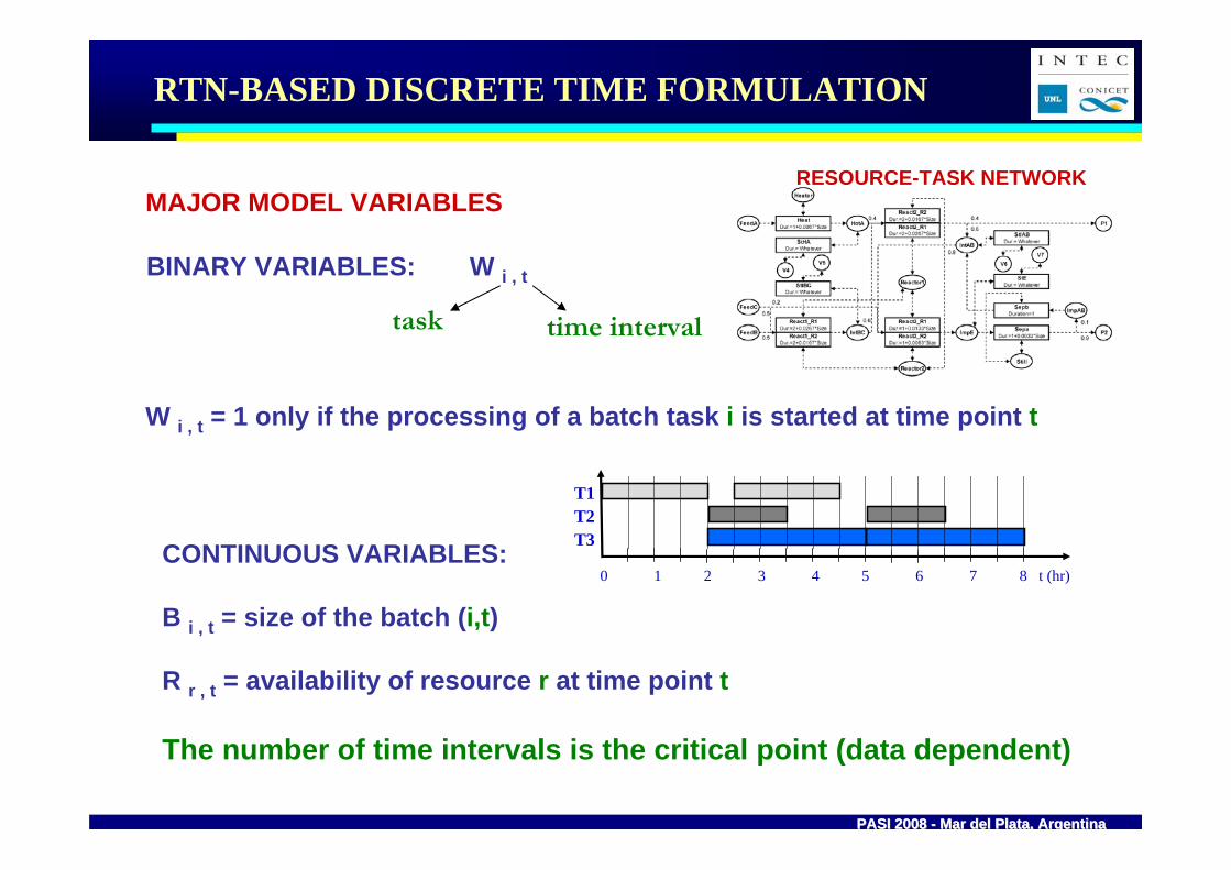
RTN-BASED DISCRETE TIME FORMULATION
MAJOR MODEL VARIABLES
BINARY VARIABLES: W i , t
task time interval
W i , t = 1 only if the processing of a batch task i is started at time point t
CONTINUOUS VARIABLES:
B i , t = size of the batch (i,t)
R r , t = availability of resource r at time point t
T1T2T3
0 1 2 3 4 5 6 7 8 t (hr)
The number of time intervals is the critical point (data dependent)
RESOURCE-TASK NETWORK

PASI 2008 PASI 2008 -- Mar del Plata, ArgentinaMar del Plata, Argentina
RTN-BASED DISCRETE TIME FORMULATION
trrtrt RR ,max0 ∀≤≤
RESOURCE BALANCE
( ) trrtIi
pt
tttiirtttiirttrrt
r
i
BvWRR ,0'
)'(')'('1 )( ∀∏+++= ∑ ∑∈ =
−−− μ
tJiRriitirititir WVBWV ,,
maxmin∈∀≤≤ BATCH SIZE
Changeovers must be defined as additional tasks

PASI 2008 PASI 2008 -- Mar del Plata, ArgentinaMar del Plata, Argentina
STN-BASED CONTINUOUS TIME FORMULATION (GLOBAL TIME POINTS)
(Pantelides, 1996; Zhang and Sargent, 1996; Mockus and Reklaitis,1999; Mockus and Reklaitis, 1999; Lee et al., 2001, Giannelos and Georgiadis, 2002; Maravelias and Grossmann, 2003)
• Define a common time grid for all shared resources • The maximum number of time points is predefined• The time at which each time point takes place is a model decision (continuous domain)• Tasks allocated to a certain time point n must start at the same time• Only zero wait tasks must finish at a time point, others may finish before
ADVANTAGES • Significant reduction in model size when the minimum number of time points is predefined• Variable processing times• A wide variety of scheduling aspects can be considered• Resource constraints are only monitored at each time point
DISADVANTAGES• Definition of the minimum number of time points• Model size and complexity depend on the number of time points predefined• Sub-optimal or infeasible solution can be generated if the number of time points is smaller than required
Continuous Time Representation IIContinuous Time Representation I
0 1 2 3 4 5 6 7 8 t (hr)
T1T2T3
0 1 2 3 4 5 6 7 8 t (hr)
T1T2T3

PASI 2008 PASI 2008 -- Mar del Plata, ArgentinaMar del Plata, Argentina
STN-BASED CONTINUOUS TIME FORMULATION
MAJOR MODEL VARIABLES
BINARY VARIABLES: Ws i , n = 1 only if task i starts at time point nWf i , n = 1 only if task i ends at time point n
CONTINUOUS VARIABLES:
T n = time for events allocated at time point nTs i , n = start time of task i assigned at time point nTf i , n = end time of task i assigned at time point nBs i , n = batch size of task i when it starts at time point nBp i , n = batch size of task i at an intermediate time point nBf i , n = batch size of task i when it ends at time point nS s , n = inventory of state s at time point nR r , n = availability of resource r at time point n
The number of time points n is the critical point
STATE-TASK NETWORK
0 1 2 3 4 5 6 7 8 t (hr)
T1T2T3

PASI 2008 PASI 2008 -- Mar del Plata, ArgentinaMar del Plata, Argentina
STN-BASED CONTINUOUS FORMULATION (GLOBAL TIME POINTS)
njWsIji
in ,1 ∀≤∑∈
njWfIji
in ,1 ∀≤∑∈
iWfWsn
inn
in ∀=∑∑
njWfWsjIi nn
inin ,1)('
'' ∀≤−∑∑∈ ≤
niWsVBsWsV iniinini ,maxmin ∀≤≤
niWfVBfWfV iniinini ,maxmin ∀≤≤
niWfWsV
BpWfWsV
nnin
nnini
innn
innn
ini
, '
''
'max
''
''
min
∀⎟⎠
⎞⎜⎝
⎛−
≤≤⎟⎠
⎞⎜⎝
⎛−
∑∑
∑∑
≤<
≤<
1,)1(1 >∀+=+ −− niBfBpBpBs ininniin
1,)1( >∀+−= ∑∑∈∈
− nsBfBsSSps
cs Ii
inp
isIi
incisnssn ρρ
nsCS ssn ,max ∀≤
nrBfWfBsWsRRi
nip
irnip
iri
nicirni
cirnrrn ,)1( ∀+++−= ∑∑− νμνμ
nTT nn ∀≥+1
niWsHBsWsTTf ininiininin ,)1( ∀−+++≤ βα
niWsHBsWsTTf ininiininin ,)1( ∀−−++≥ βα
1,)1()1( >∀−+≤− niWfHTTf innni
1,)1()1( >∈∀−−≥− nIiWfHTTf ZWinnni
nIiIijclTfTs jjiinini ,',,')1(' ∈∈∀+≥ −
nJjV T
Ssjsn
j
,1 ∈∀≤∑∈
nSsJjVCS jT
jsnjsjn ,, ∈∈∀≤
nSsSS T
Jj
sjnsnTs
,∈∀= ∑∈
ALLOCATION CONSTRAINTS
BATCH SIZE CONSTRAINTS
SHARED STORAGE TASKS
TIMING AND SEQUENCING CONSTRAINTS
MATERIAL AND RESOURCE BALANCES
(Maravelias and Grossmann, 2003)

PASI 2008 PASI 2008 -- Mar del Plata, ArgentinaMar del Plata, Argentina
RTN-BASED CONTINUOUS TIME FORMULATION
MAJOR MODEL VARIABLES
BINARY VARIABLES: W i , n ,n’ = 1 only if task i starts at time point n
and finishes at time point n’
CONTINUOUS VARIABLES:
T n = time for events allocated at time point nB i , n, n’ = batch size of task i when it starts at time point n
and finishes at time point n’R r , n = availability of resource r at time point n
The number of time points n is the critical point
0 1 2 3 4 5 6 7 8 t (hr)
T1T2T3
RESOURCE-TASK NETWORK
PASI 2008 PASI 2008 -- Mar del Plata, ArgentinaMar del Plata, Argentina
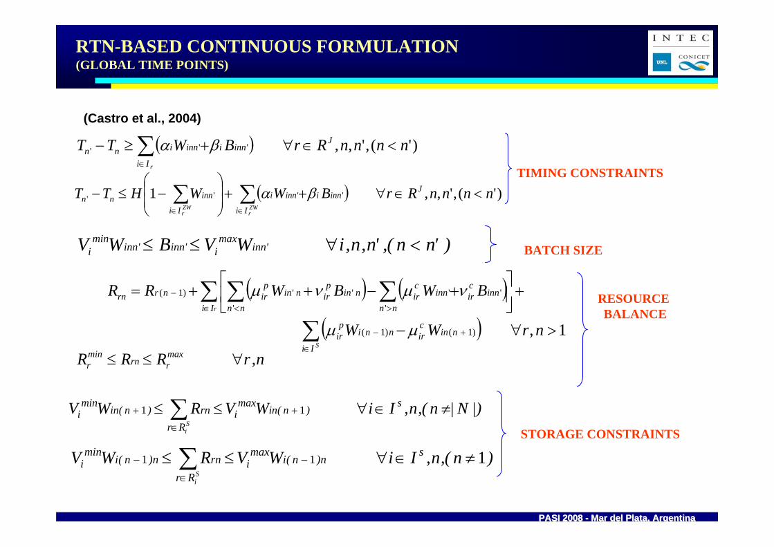
RTN-BASED CONTINUOUS FORMULATION (GLOBAL TIME POINTS)
( ) )'(,',,''' nnnnRrBWTT J
Ii
inniinninnr
<∈∀+≥− ∑∈
βα
( ) )'(,',,1 '''' nnnnRrBWWHTT J
Ii
inniinni
Ii
innnnZWr
ZWr
<∈∀++⎟⎟⎠
⎞⎜⎜⎝
⎛−≤− ∑∑
∈∈
βα
)'nn(,'n,n,iWVBWV 'innmax
i'inn'innmin
i <∀≤≤
( ) ( )( ) 1, )1()1(
'
''
'
'')1(
>∀−
+⎥⎦
⎤⎢⎣
⎡+−++=
∑
∑ ∑∑
∈
+−
∈ ><
−
nrWW
BWBWRR
S
r
Ii
nincirnni
pir
Ii nn
inncirinn
cir
nn
ninp
irninp
irnrrn
μμ
νμνμ
n,rRRR maxrrn
minr ∀≤≤
|)N|n(,n,IiWVRWV s)n(in
maxi
Rrrn)n(in
mini
Si
≠∈∀≤≤ +
∈
+ ∑ 11
)n(,n,IiWVRWV sn)n(i
maxi
Rrrnn)n(i
mini
Si
111 ≠∈∀≤≤ −
∈
− ∑
TIMING CONSTRAINTS
BATCH SIZE
RESOURCEBALANCE
STORAGE CONSTRAINTS
(Castro et al., 2004)

PASI 2008 PASI 2008 -- Mar del Plata, ArgentinaMar del Plata, Argentina
STN-BASED CONTINUOUS FORMULATION (UNIT-SPECIFIC TIME EVENT)
MAIN ASSUMPTIONS• The number of event points is predefined• Event points can take place at different times in different units (global time is relaxed)
ADVANTAGES • More flexible timing decisions• Less number of event points
DISADVANTAGES• Definition of event points• More complicated models, no reference points to check resource availabilities• Model size and complexity depend on the number of time points predefined• Sub-optimal or infeasible solution can be generated if the number of time points is smaller than required • Additional tasks for storage and utilities
Event-Based Representation
(Ierapetritou and Floudas, 1998; Vin and Ierapetritou, 2000; Lin et al., 2002; Janak et al., 2004).
12
32
0 1 2 3 4 5 6 7 8 t (hr)
32J1
J2J3

PASI 2008 PASI 2008 -- Mar del Plata, ArgentinaMar del Plata, Argentina
STN-BASED CONTINUOUS TIME FORMULATION(UNIT-SPECIFIC TIME EVENT)
MAJOR MODEL VARIABLESBINARY VARIABLES:
W i , n = 1 only if task i starts at time point nWs i , n = 1 only if task i starts at time point nWf i , n = 1 only if task i ends at time point n
CONTINUOUS VARIABLES:
T n = time for events allocated at time point nTs i , n = start time of task i assigned at time point nTf i , n = end time of task i assigned at time point nBs i , n = batch size of task i when it starts at time point nB i , n = batch size of task i at an intermediate time point nBf i , n = batch size of task i when it ends at time point nS s , n = inventory of state s at time point nR i ,r , n = amount of resource r consumed by task i at time point nR Ar , n = availability of resource r at time point n
The number of time events n is the critical point
STATE-TASK NETWORK
0 1 2 3 4 5 6 7 8 t (hr)
T1T2T3

PASI 2008 PASI 2008 -- Mar del Plata, ArgentinaMar del Plata, Argentina
STN-BASED CONTINUOUS FORMULATION (UNIT-SPECIFIC TIME EVENT)
n,jWjIi
in ∀≤∑∈
1
niWWfWs innn
innn
in ,'
''
' ∀=−∑∑<≤
iWfWsn
inn
in ∀= ∑∑n,iWfWsWs
n'n'in
n'n'in
nin ∀+−≤ ∑∑∑
<<
1
niWfWsWfnn
innn
inin ,'
''
' ∀−≤ ∑∑<<
ALLOCATION CONSTRAINTS
n,iWVBWV inmaxiinin
mini ∀≤≤
( ) 1, 1 )1()1(max
)1( >∀+−−≤ −−− niWfWVBB niniiniin
( ) 1, 1 )1()1(max
)1( >∀+−−≥ −−− niWfWVBB niniiniin
niBBs inin , ∀≤niWsVBBs iniinin , max ∀+≤
( ) niWsVBBs iniinin , 1 max ∀−−≥n,iBBf inin ∀≤
niWfVBBf iniinin , max ∀+≤
( ) niWfVBBf iniinin , 1 max ∀−−≥
MATERIAL BALANCEnsBBsBBfSS
sts
stst
cs
STs
stst
ps Ii
niIi
incis
Iini
Iini
pisnssn ,
)1()1()1( ∀−−++= ∑∑∑∑∈∈∈
−∈
−− ρρ
BATCH SIZE CONSTRAINTS
nIisCB sts
stsnist ,,max ∈∀≤
STORAGE CAPACITY
(Janak et al., 2004)

PASI 2008 PASI 2008 -- Mar del Plata, ArgentinaMar del Plata, Argentina
STN-BASED CONTINUOUS FORMULATION (UNIT-SPECIFIC TIME EVENT)
TIMING AND SEQUENCING
CONSTRAINTS (PROCESSING TASKS)
niTsTf inin , ∀≥
niH WTsTf ininin , ∀+≤( ) 1, 1 )1()1()1( >∀+−+≤ −−− niWfWH TfTs nininiin
( ) ( )
)'(,',,
1 1'''
''''
nnnni
WfH WfH WsH BWsTsTfnnn
ininininiiniinin
≤∀
⎟⎠
⎞⎜⎝
⎛+−+−++≥− ∑
≤≤
βα
1, )1( >∀≥ − niTfsT nini
( ) 1,,',', 1 ')1('')1(' >∈≠∀−−++≥ −− nJjiiiiWsWfHclTfsT iiinniiinini
( ) 1,',',,',, 1 ')1(')1(' >≠∈∈∈∈∀−+≥ −− njjJjJjIiIisWfHTfsT iip
scsninini
( )1,',',,',,
2
'
)1(')1('
>≠∈∈∈∈∈∀
−−+≤ −−
njjJjJjIiIiSs
WsWfHTfsT
iips
cs
ZW
inninini
( ) ( )
)'(,',,
1 1'''
''''
nnnnIi
WfH WfH WsH BWsTsTf
ZW
nnnininininiiniinin
≤∈∀
⎟⎠
⎞⎜⎝
⎛+−+−++≤− ∑
≤≤
βα

PASI 2008 PASI 2008 -- Mar del Plata, ArgentinaMar del Plata, Argentina
STN-BASED CONTINUOUS FORMULATION (UNIT-SPECIFIC TIME EVENT)
TIMING AND SEQUENCING CONSTRAINTS (STORAGE TASKS)
niTsTf stnini stst , ∀≥
( ) 1,,, 1 )1()1( >∈∈∀−−≥ −− nIiIisWfHTfsT STs
stpsnininist
( ) 1,,, 1 )1()1( >∈∈∀−+≤ −− nIiIisWfHTfsT STs
stpsnininist
1,,, )1( >∈∈∀≥−
nIiIisTfsT STs
stcsnini st
( ) 1,,, 1)1( >∈∈∀−+≤−
nIiIisWsHTfsT STs
stcsinnini st
1, )1( >∀=−
niTfsT stnini stst
n,Ii,rBWR rnicirni
cirirn ∈∀+= νμ
1,max =∀=+∑∈
nrRRR rArn
Iiirn
r
1,)1()1( >∀+=+ −∈
−∈
∑∑ nrRRRR Anr
Iinir
Arn
Iiirn
rr
nrTsTf rnnr , ∀≥( ) 1,, 1 )1()1()1( >∈∀+−−≥ −−− nIirWfWHTsfT rninirnni
( ) 1,, 1 )1()1( >∈∀−−≤ −− nIirWHTsfT rnirnni
( ) nIirWHTssT rininrn ,, 1 ∈∀−−≥( ) nIirWHTssT rininrn ,, 1 ∈∀−+≤
1, )1( >∀= − nrTfsT nrrn
RESOURCE BALANCE
TIMING AND SEQUENCING OF RESOURCE USAGE

PASI 2008 PASI 2008 -- Mar del Plata, ArgentinaMar del Plata, Argentina
Task 1U1
Task 1U1
Task 2U2
Task 2U2
Task 3U3
Task 3U3
Tasks 4-7 U4
Tasks 4-7 U4
Tasks 13-17
U8/U9
Tasks 13-17
U8/U9
Tasks 10-12
U6/U7
Tasks 10-12
U6/U7
Tasks 8,9U5
Tasks 8,9U5
1 2 4 57
11
10
9
8
6
3
12
15
19
18
17
16
zw
zw
zw
14
13
zw0.5
0.31
0.2 – 0.7
0.5
CASE STUDY: CASE STUDY: WestenbergerWestenberger & & KallrathKallrath (1995)(1995)
Benchmark problem for production scheduling in chemical industry
COMPARISON OF DISCRETE AND CONTINUOUS TIME FORMULATIONS(STN-BASED FORMULATIONS )

PASI 2008 PASI 2008 -- Mar del Plata, ArgentinaMar del Plata, Argentina
17 processing tasks, 19 states 9 production units37 material flowsBatch mixing / splittingCyclical material flowsFlexible output proportionsNon-storable intermediate productsNo initial stock of final products Unlimited storage for raw material and final productsSequence-dependent changeover times
Task 1U1
Task 1U1
Task 2U2
Task 2U2
Task 3U3
Task 3U3
Tasks 4-7 U4
Tasks 4-7 U4
Tasks 13-17
U8/U9
Tasks 13-17
U8/U9
Tasks 10-12
U6/U7
Tasks 10-12
U6/U7
Tasks 8,9U5
Tasks 8,9U5
1 2 4 57
11
10
9
8
6
3
12
15
19
18
17
16
zw
zw
zw
14
13
zw0.5
0.31
0.2 – 0.7
0.5
Task 1U1
Task 1U1
Task 2U2
Task 2U2
Task 3U3
Task 3U3
Tasks 4-7 U4
Tasks 4-7 U4
Tasks 13-17
U8/U9
Tasks 13-17
U8/U9
Tasks 10-12
U6/U7
Tasks 10-12
U6/U7
Tasks 8,9U5
Tasks 8,9U5
1 2 4 57
11
10
9
8
6
3
12
15
19
18
17
16
zw
zw
zw
14
13
zw0.5
0.31
0.2 – 0.7
0.5
PROBLEM FEATURES

PASI 2008 PASI 2008 -- Mar del Plata, ArgentinaMar del Plata, Argentina
MAKESPAN MINIMIZATION
Instance A B Formulation Discrete Continuous Discrete Continuous time points 30 8 9 30 7 8 binary variables 720 384 432 720 336 384 continuous variables 3542 2258 2540 3542 1976 2258 constraints 6713 4962 5585 6713 4343 4964 LP relaxation 9.9 24.2 24.1 9.9 25.2 24.3 objective 28 28 28 28 32 30 iterations 728 78082 27148 2276 58979 2815823 nodes 10 1180 470 25 1690 63855 CPU time (s) 1.34 108.39 51.41 4.41 66.45 3600.21 relative gap 0.0 0.0 0.0 0.0 0.0 0.067
20
00
2020 20
020
020

PASI 2008 PASI 2008 -- Mar del Plata, ArgentinaMar del Plata, Argentina
MAKESPAN MINIMIZATION
Discrete modelTime intervals: 30
Makespan: 28
Continuous modelTime points: 7Makespan: 32

PASI 2008 PASI 2008 -- Mar del Plata, ArgentinaMar del Plata, Argentina
PROFIT MAXIMIZATION
H = 24 h
10
105
1010
Instance D Discrete Continuous Formulation LB UB time points 240 24 24 14 binary variables 5760 576 576 672 continuous variables 28322 2834 2834 3950 constraints 47851 4794 4799 8476 LP relaxation 1769.9 1383.0 2070.9 1647.1 objective 1425.8 1184.2 1721.8 1407.4 iterations 449765 3133 99692 256271 nodes 5580 203 4384 1920 CPU time (s) 7202 6.41 58.32 258.54 relative gap 0.122 0.047 0.050 0.042

PASI 2008 PASI 2008 -- Mar del Plata, ArgentinaMar del Plata, Argentina
H = 24 h
Time intervals: 240Profit: 1425.8
Time points: 14Profit: 1407.4
Discrete model Continuous model
PROFIT MAXIMIZATION

PASI 2008 PASI 2008 -- Mar del Plata, ArgentinaMar del Plata, Argentina
ROAD-MAP FOR OPTIMIZATION APPROACHES
EVENT REPRESENTATION
NETWORK-ORIENTED PROCESSESDISCRETE TIME
- Global time intervals (STN or RTN)CONTINUOUS TIME
- Global time points (STN or RTN)- Unit- specific time event (STN)
BATCH-ORIENTED PROCESSESCONTINUOUS TIME
- Time slots- Unit-specific direct precedence- Global direct precedence- Global general precedence
Main events involve changes in: Processing tasks (start and end)Availability of any resourceResource requirement of a task
Key point: reference points
to check resources
Key point: arrange resource
utilization
PASI 2008 PASI 2008 -- Mar del Plata, ArgentinaMar del Plata, Argentina
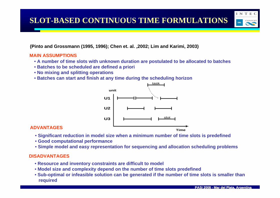
SLOT-BASED CONTINUOUS TIME FORMULATIONS
MAIN ASSUMPTIONS• A number of time slots with unknown duration are postulated to be allocated to batches• Batches to be scheduled are defined a priori• No mixing and splitting operations• Batches can start and finish at any time during the scheduling horizon
ADVANTAGES • Significant reduction in model size when a minimum number of time slots is predefined• Good computational performance• Simple model and easy representation for sequencing and allocation scheduling problems
DISADVANTAGES• Resource and inventory constraints are difficult to model• Model size and complexity depend on the number of time slots predefined• Sub-optimal or infeasible solution can be generated if the number of time slots is smaller than
required
slot
U1
U3
U2
unit
Time
task
(Pinto and Grossmann (1995, 1996); Chen et. al. ,2002; Lim and Karimi, 2003)

PASI 2008 PASI 2008 -- Mar del Plata, ArgentinaMar del Plata, Argentina
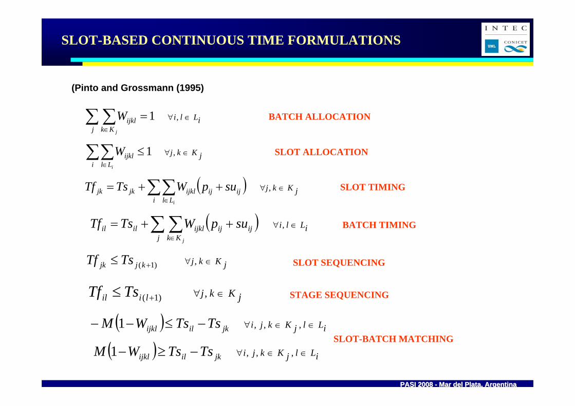
SLOT-BASED CONTINUOUS TIME FORMULATION
MAJOR MODEL VARIABLES
BINARY VARIABLES: W i , j , k , l
batchunit
slot
W i , j , k, l = 1 only if stage l of batch i is allocated to slot k of unit j
CONTINUOUS VARIABLES:
Ts i , l = start time of stage l of batch iTf i , l = end time of stage l of batch I
Ts j , k = start time of slot k in unit jTf j , k = end time of slot k in unit j
The number of time slots k is the critical point
stagea c
e b
dt1t2J1
J2
t3t1t2t3
PASI 2008 PASI 2008 -- Mar del Plata, ArgentinaMar del Plata, Argentina
iLlij Kk
ijklj
W ∈∀=∑ ∑∈
, 1
jKkji Ll
ijkli
W ∈∀≤∑∑∈
, 1
( ) jKkji Ll
ijijijkljkjki
supWTsTf ∈∀∑∑∈
++= ,
( ) iLlij Kk
ijijijklililj
supWTsTf ∈∀∑ ∑∈
++= ,
jKkjkjjk TsTf ∈∀+≤ , )1(
jKkjliil TsTf ∈∀+≤ , )1(
( ) iLljKkjijkilijkl TsTsWM ∈∈∀−≤−− ,,, 1
( ) iLljKkjijkilijkl TsTsWM ∈∈∀−≥− ,,, 1
BATCH ALLOCATION
SLOT TIMING
SLOT ALLOCATION
BATCH TIMING
SLOT SEQUENCING
STAGE SEQUENCING
SLOT-BATCH MATCHING
(Pinto and Grossmann (1995)
SLOT-BASED CONTINUOUS TIME FORMULATIONS

PASI 2008 PASI 2008 -- Mar del Plata, ArgentinaMar del Plata, Argentina
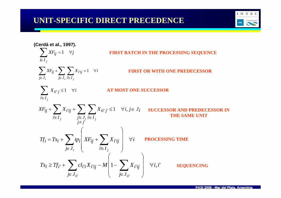
UNIT-SPECIFIC DIRECT PRECEDENCE
MAIN ASSUMPTIONS
ADVANTAGES • Sequencing is explicitly considered in model variables• Changeover times and costs are easy to implement
DISADVANTAGES• Large number of sequencing variables• Resource and material balances are difficult to model
(Cerdá et al., 1997).
• Batches to be scheduled are defined a priori• No mixing and splitting operations • Batches can start and finish at any time during the scheduling horizon
J
J’
UNITS
Time
2 3 5
1 4 6
X 1,4,J’ =1
X 2,3,J =1 X 3,5,J =1
X 4,6,J =1
6 BATCHES, 2 UNITS
6 x 5 x 2= 60 SEQUENCING VARIABLES

PASI 2008 PASI 2008 -- Mar del Plata, ArgentinaMar del Plata, Argentina
MAJOR MODEL VARIABLES
BINARY VARIABLES: X i , i’ , j
batchbatch
unit
X i , i’ , j = 1 only if batch i’ is processed immediately after that batch i in unit j
Xf i , j = 1 only if batch i is first processed in unit j
CONTINUOUS VARIABLES:
Ts i = start time of batch iTf i = end time of batch i
The number of predecessors and units is the critical point
UNIT-SPECIFIC DIRECT PRECEDENCE
J
J’
UNITS
Time
2 3 5
1 4 6
X 1,4,J’ =1
X 2,3,J =1 X 3,5,J =1
X 4,6,J =1
PASI 2008 PASI 2008 -- Mar del Plata, ArgentinaMar del Plata, Argentina
UNIT-SPECIFIC DIRECT PRECEDENCE
FIRST BATCH IN THE PROCESSING SEQUENCE
AT MOST ONE SUCCESSOR
FIRST OR WITH ONE PREDECESSOR
SUCCESSOR AND PREDECESSOR IN THE SAME UNIT
PROCESSING TIME
SEQUENCING
jXF
jIiij ∀=∑
∈
1
iXXF
i ji Jj Iiiji
Jjij ∀=+∑ ∑∑
∈ ∈∈
1 '
'
iX
jIijii ∀≤∑
∈
1 '
'
iJjiXXXF
jjJj Ii
jiiIi
ijiij
i jj
∈∀≤++ ∑ ∑∑≠∈ ∈∈
, 1
'' '
'''
'
iXXFtpTsTf
ji Iiijiij
Jjiii ∀
⎟⎟⎟⎟
⎠
⎞
⎜⎜⎜⎜
⎝
⎛
++= ∑∑∈∈
'
'
', 1
''
'''' iiXMXclTfTs
iiii Jjijiiji
Jjiiii ∀
⎟⎟⎟
⎠
⎞
⎜⎜⎜
⎝
⎛−−+≥ ∑∑
∈∈
(Cerdá et al., 1997).

PASI 2008 PASI 2008 -- Mar del Plata, ArgentinaMar del Plata, Argentina
GLOBAL DIRECT PRECEDENCE
DISADVANTAGES
(Méndez et al., 2000; Gupta and Karimi, 2003)
MAIN ASSUMPTIONS
• Batches to be scheduled are defined a priori• No mixing and splitting operations• Batches can start and finish at any time during the scheduling horizon
ADVANTAGES
J
J’
UNITS
Time
2 3 5
1 4 6
Allocation variables
Y 2,J = 1; Y 3,J = 1 ; Y 5,J = 1
Y 1,J’ = 1; Y 4,J’ = 1 ; Y 6,J’ = 1
X 1,4 =1
X 2,3 =1 X 3,5 =1
X 4,6 =1
6 BATCHES, 2 UNITS
6 x 5 = 30 SEQUENCING VARIABLES
• Sequencing is explicitly considered in model variables• Changeover times and costs are easy to implement
• Large number of sequencing variables• Resource and material balances are difficult to model

PASI 2008 PASI 2008 -- Mar del Plata, ArgentinaMar del Plata, Argentina
MAJOR MODEL VARIABLES
BINARY VARIABLES: X i , i’
batchbatch
X i , i’ = 1 only if batch i’ is processed immediately after that batch i in unit jW i , J = 1 only if batch i’ is processed in unit jXf i , j = 1 only if batch i is first processed in unit j
CONTINUOUS VARIABLES:
Ts i = start time of batch iTf i = end time of batch i
The number of predecessors is the critical point
GLOBAL DIRECT PRECEDENCE
J
J’
UNITS
Time
2 3 5
1 4 6
X 1,4 =1
X 2,3 =1 X 3,5 =1
X 4,6 =1

PASI 2008 PASI 2008 -- Mar del Plata, ArgentinaMar del Plata, Argentina
GLOBAL DIRECT PRECEDENCE
AT MOST ONE FIRST BATCH IN THE PROCESSING SEQUENCE
SEQUENCING-ALLOCATION MATCHING
ALLOCATION CONSTRAINT
jXFjIi
ij ∀≤∑∈
1
iWXFii Jj
ijJj
ij ∀=+∑∑∈∈
1
''' ,', 1 iiiijiijij JjiiXWWXF ∈∀+−≤+
( )'' ,', 1 iiiiiijij JJjiiXWXF −∈∀−≤+
iXXFi
iiJj
ij
i
∀=+∑∑∈
1'
'
iXi
ii ∀≤∑ 1'
'
( ) iWXFtpTsTf ijijJj
iiii
∀++= ∑∈
( ) ( ) iXMWsuclTfTs iiJj
jijiiiiii
∀−−++≥ ∑∈
1 '''''
FIRST OR WITH ONE PREDECESSOR
AT MOST ONE SUCCESSOR
TIMING AND SEQUENCING
(Méndez et al., 2000)

PASI 2008 PASI 2008 -- Mar del Plata, ArgentinaMar del Plata, Argentina
GLOBAL GENERAL PRECEDENCE
ADVANTAGES
DISADVANTAGES
(Méndez et al., 2001; Méndez and Cerdá (2003,2004))
MAIN ASSUMPTIONS
• Batches to be scheduled are defined a priori• No mixing and splitting operations• Batches can start and finish at any time during the scheduling horizon
J
J’
UNITS
Time
2 3 5
1 4 6
Allocation variables
Y2,J = 1; Y3,J = 1 ; Y5,J = 1
Y1,J’ = 1; Y4,J’ = 1 ; Y6,J’ = 1
X1,4 =1
X1,6 =1
X2,3 =1 X3,5 =1X2,5 =1
X4,6 =1
6 BATCHES, 2 UNITS
(6*5)/2= 15 SEQUENCING VARIABLES
• General sequencing is explicitly considered in model variables• Changeover times and costs are easy to implement• Lower number of sequencing decisions• Sequencing decisions can be extrapolated to other resources
• Material balances are difficult to model, no reference points

PASI 2008 PASI 2008 -- Mar del Plata, ArgentinaMar del Plata, Argentina
MAJOR MODEL VARIABLES
BINARY VARIABLES: X i , i’
batchbatch
X i , i’ = 1 only if batch i’ is processed after that batch i in unit jW i , J = 1 only if batch i’ is processed in unit j
CONTINUOUS VARIABLES:
Ts i = start time of batch iTf i = end time of batch i
The number of predecessors is the critical point
GLOBAL GENERAL PRECEDENCE
J
J’
UNITS
Time
2 3 5
1 4 6
X1,4 =1
X1,6 =1
X2,3 =1 X3,5 =1X2,5 =1
X4,6 =1
CAN BE EASILY GENERALIZED TO MULTISTAGE PROCESSES
AND TO SEVERAL RESORCES

PASI 2008 PASI 2008 -- Mar del Plata, ArgentinaMar del Plata, Argentina
GLOBAL GENERAL PRECEDENCE
SEQUENCING CONSTRAINTS
ALLOCATION CONSTRAINT
PROCESSING TIME
iLliW
ilJjilj ∈∀=∑
∈
, 1
iLliWtpTsTf iljJj
iljilil
il
∈∀+= ∑∈
,
( ) ( ) '',''''','''','' ,',,', 2 1 liiliijliiljliilliliililli JjLlLliiWWMXMsuclTfTs ∈∈∈∀−−−−−++≥
( ) '',''''',,'''' ,',,', 2 liiliijliiljliilililliliil JjLlLliiWWMXMsuclTfTs ∈∈∈∀−−−−++≥
1,, )1( >∈∀≥ − lLliTfTs iliil STAGE PRECEDENCE
(Méndez and Cerdá, 2003)

PASI 2008 PASI 2008 -- Mar del Plata, ArgentinaMar del Plata, Argentina
SUMMARY OF OPTIMIZATION APPROACHES
Time representation
DISCRETE CONTINUOUS
Event representation
Global time intervals
Global time points
Unit-specific time events
Time slots* Unit-specific immediate
precedence*
Immediate precedence*
General precedence*
Main decisions ------------------- Lot-sizing, allocation, sequencing, timing ------------------
-------- Allocation, sequencing, timing ----------
Key discrete variables
Wijt defines if task I starts in unit j at the beginning of time
interval t.
Wsin / Wfin define if task i starts/ends at time point
n. Winn’ defines if task i starts at time point n and ends at time point n’.
Wsin /Win / Wfin define if
task i starts/is
active/ends at event point n.
Wijk define if unit j starts task i at the beginning of time slot k.
Xii’j defines if batch i is processed
right before of batch i’ in
unit j. XFij defines if batch i starts
the processing sequence of
unit j.
Xii’ defines if batch i is processed
right before of batch i’. XFij / Wij defines if
batch i starts/is
assigned to unit j.
X’ii’ define if batch i is processed before or
after of batch i’. Wij
defines if batch i is
assigned to unit j
Type of process
---------------------------------- General network ---------------------------------
----------------------- Sequential ---------------------
Material balances
Network flow equations
(STN or RTN)
Network flow equations (STN or RTN)
--- Network flow equations --- (STN)
-------------------- Batch-oriented ------------------
Critical modeling
issues
Time interval duration, scheduling
period (data dependent)
Number of time points (iteratively estimated)
Number of time events (iteratively estimated)
Number of time slots
(estimated)
Number of batch tasks
sharing units (lot-sizing) and units
Number of batch tasks
sharing units (lot-sizing)
Number of batch tasks
sharing resources
(lot-sizing)
Critical problem features
Variable processing time, sequence-
dependent changeovers
Intermediate due dates and raw-material
supplies
Intermediate due dates and raw-material
supplies
Resource limitations
Inventory, resource
limitations
Inventory, resource
limitations
Inventory

PASI 2008 PASI 2008 -- Mar del Plata, ArgentinaMar del Plata, Argentina
RESOURCE-CONSTRAINED EXAMPLE
12 batches and 4 processing units in parallel Manpower limitations (4 , 3 , 2 operators crews)Specific batch due dates Total earliness minimization Three approaches: time-slots, general precedence and event times

PASI 2008 PASI 2008 -- Mar del Plata, ArgentinaMar del Plata, Argentina
(a) without manpower limitation (b) 3 operator crews (c) 2 operators crews
COMPUTATIONAL RESULTS
Case Study Event representation Binary vars, cont. vars, constraints
Objective function
CPU time Nodes
2.a Time slots & preordering 100, 220, 478 1.581 67.74a 456 General precedence 82, 12, 202 1.026 0.11b 64 Unit-based time events (4) 150, 513, 1389 1.026 0.07c 7
2.b Time slots & preordering 289, 329, 1156 2.424 2224a 1941 General precedence 127, 12, 610 1.895 7.91b 3071 Unit-based time events (12) 458, 2137, 10382 1.895 6.53c 1374
2.c Time slots & preordering 289, 329, 1156 8.323 76390a 99148 General precedence 115, 12, 478 7.334 35.87b 19853 Unit-based time events (12) 446, 2137, 10381 7.909 178.85c 42193

PASI 2008 PASI 2008 -- Mar del Plata, ArgentinaMar del Plata, Argentina
TIGHTENING CONSTRAINTS
MAJOR GOAL
Use additional constraints to
Obtain a good estimation of problem variables related to the objective function (makespan, tardiness, earliness)
Accelerate the pruning process by producing a better estimation on the RMIP solution value at each node
Exploit the information provided by 0-1 decision variables
Reduce computational effort

PASI 2008 PASI 2008 -- Mar del Plata, ArgentinaMar del Plata, Argentina
MOTIVATING EXAMPLES
SCHEDULING OF A SINGLE-STAGE BATCH PLANT
OBJECTIVE: MINIMUM MAKESPAN
If unit-dependent setup times are required
where
is a better estimation of the jth-unit ready time because it also considers the release times of the candidate tasks for unit j.
( ) MKYptsurujIi
ijijijj ≤++∑∈
∗ Jj∈∀
[ ]⎥⎦
⎤⎢⎣
⎡−=
∈
∗iji
Iijj surtruru
j
Min,Max
The estimation for makespan is based only on assignment variables.

PASI 2008 PASI 2008 -- Mar del Plata, ArgentinaMar del Plata, Argentina
MOTIVATING EXAMPLES
SCHEDULING OF A SINGLE-STAGE BATCH PLANT
OBJECTIVE: MINIMUM MAKESPAN
If sequence-dependent setup times are required
where
Jj∈∀
[ ]⎥⎦
⎤⎢⎣
⎡−=
∈
∗iji
Iijj surtruru
j
Min,Max
( ) MKYptsuru ijIi
ijijMinij
MinijIij
jj
≤+++− ∑∈
∈σσ ][Max*
[ ]ijiiiIi
Minij
j'':'
Min τσ≠∈
=
The estimation for makespan is based only on assignment variables.

PASI 2008 PASI 2008 -- Mar del Plata, ArgentinaMar del Plata, Argentina
COMPUTATIONAL RESULTS
Example 1A: Sequence independent setup times
Example 1B: Sequence dependent setup times
n Binary vars,
Continuous vars, Constraints Objective
Function Relative Gap (%)
CPU time (sec.) Nodes Objective
FunctionRelative Gap (%)
CPU time (sec.) Nodes
12 82, 25, 214 8.428 - 19.03 94365 8.645 - 8.36 39350 16 140, 33, 382 12.353 2.43 3600 † 8893218 12.854 - 1188.50 3421982 18 161, 37, 444 13.985 - 2872.81 7166701 14.633 27.07 3600 † 8708577 20 201, 41, 558 15.268 22.62 3600 † 6282059 15.998 21.95 3600 † 6570231
WITHOUT TIGHTENING CONSTRAINTS
p ( ) ( ) p ( ) ( )
12 82, 25, 218 8.428 - 0.05 12 8.645 - 0.05 15 16 140, 33, 386 12.353 - 0.03 1 12.854 - 0.09 44 18 161, 37, 448 13.985 - 0.11 27 14.611 - 40.36 116413 20 201, 41, 562 15.268 - 0.14 21 15.998 - 183.56 417067 22 228, 45, 622 15.794 - 0.20 49 16.396 - 167.09 359804 25 286, 51, 792 18.218 - 0.42 110 19.064 * - 79.25 109259 29 382, 59, 1064 23.302 - 0.61 82 24.723 * - 5.92 5385 35 532, 71, 1430 26.683 - 0.97 90 40 625, 81, 1656 28.250 - 0.91 34
WITH TIGHTENING CONSTRAINTS
Marchetti, P. A. and Cerdá, J., Submitted 2007

PASI 2008 PASI 2008 -- Mar del Plata, ArgentinaMar del Plata, Argentina
MULTISTAGE MULTIPRODUCT BATCH PROCESS
Major problem features (Pharmaceutical industry) 17 processing units5 processing stages30 to 300 production orders per week (thousands of batch operations)Different processing times (0.2 h to 3 h)Sequence-dependent changeovers (0.5 h to 2 h)Allocation restrictionsFew minutes to generate the scheduleRescheduling on a daily basis
SOLUTION OF A LARGE-SCALE MULTISTAGE PROCESS
1
2
3
4
5
7
8
9
10
11
12
13
14
6
16
17
15

PASI 2008 PASI 2008 -- Mar del Plata, ArgentinaMar del Plata, Argentina
PROPOSED TWO-STAGE SOLUTION STRATEGY
FIRST STAGE: CONSTRUCTIVE STAGE
SECOND STAGE: IMPROVEMENT STAGE
BASED ON A REDUCED MILP-BASED MODELGENERATE THE BEST POSSIBLE SCHEDULE IN A SHORT-TIMEOPTION: GENERATE A FULL SCHEDULE BY INSERTING ORDERS ONE BY ONE
BASED ON A REDUCED MILP-BASED MODEL
IMPROVE THE INITIAL SCHEDULE BY LOCAL RE-ASSIGNMENTS AND RE-SEQUENCING
SOLUTION STRATEGY

PASI 2008 PASI 2008 -- Mar del Plata, ArgentinaMar del Plata, Argentina
GENERAL MILP MODEL
SEQUENCING CONSTRAINTS
ALLOCATION CONSTRAINT
PROCESSING TIME
iLliW
ilJjilj ∈∀=∑
∈
, 1
iLl,iiljJj
iljilil Wtp TsTfil
∈∀
∈∑+=
( ) ( ) '',''''','''','' ,',,', 2 1 liiliijliiljliilliliililli JjLlLliiWWMXMsuclTfTs ∈∈∈∀−−−−−++≥
( ) '',''''',,'''' ,',,', 2 liiliijliiljliilililliliil JjLlLliiWWMXMsuclTfTs ∈∈∈∀−−−−++≥
1,, )1( >∈∀≥ − lLliTfTs iliil STAGE PRECEDENCE
(Méndez and Cerdá, 2003) Multistage multipurpose batch plant
General problem representation

PASI 2008 PASI 2008 -- Mar del Plata, ArgentinaMar del Plata, Argentina
SCHEDULE FOR 30-ORDER PROBLEM
TOTAL COMPUTATIONAL
EFFORT
FEW MINUTES
BEST SCHEDULE

PASI 2008 PASI 2008 -- Mar del Plata, ArgentinaMar del Plata, Argentina
CPU-limit (s) Makespan (h) CPUs
Orders Ap. NPS Per phase Constructive
Stage
Improvement
stage
Scheduling Total
30 AP2 1 (10);(10) 33.149 31.175 86.4 188
30 AP2 2 (20);(10) 32.523 31.007 175 275
30 AP2 3 (30);(10) 34.447 31.787 255 355
50 AP2 1 (10);(10) 52.911 51.275 240 342
50 AP2 2 (15);(10) 52.964 51.080 321 429
50 AP3 3 (20);(10) 55.705 52.960 306 407
Model Bin. vars. Cont. vars. Cons. RMIP MIP Best possible CPUs Nodes
MILP 2521 2708 10513 7.449 47.982 13.325 3600 62668
CP - 1050 1300 - 79.989 - 3600 1432
COMPUTATIONAL RESULTS
Pure optimization approaches
Proposed solution strategy

PASI 2008 PASI 2008 -- Mar del Plata, ArgentinaMar del Plata, Argentina
REMARKS
Different performance depending on the objective function.
Discrete-time models may be computationally more effective than continuous-time
Difficult selection of the number of time or event points in the general continuous-time formulation.
General continuous-time models become quickly computationally intractable for scheduling of medium complexity process networks.
Problems with more than 150 time intervals are usually difficult to solve by usingdiscrete time models.
Problems with more than 15 time or event points appear intractable for continuous time models.
Current optimization models are able to solve complex scheduling problems
Small examples can be solved to optimality
Discrete-time models are usually more flexible than continuous-time models

PASI 2008 PASI 2008 -- Mar del Plata, ArgentinaMar del Plata, Argentina
CONCLUSIONS
Batch-oriented models can incorporate practical process knowledge in a more natural way
Batch-oriented continuous models are more efficient for sequential processes and larger number of batches
Combine other approaches with mathematical programming for solving large scale problems looks very promising
Inventory constraints seem very difficult to address without point references
Resource constraints can be efficiently addressed without point references