1

Shor t Tutor ial on Matlab(©2004, 2005 by Tomas Co)

Par t 3. Simulink® Basics

1. A simple example.

Suppose you want to model the response of a first order process model given by thefollowing equation:

( )

o

in

TT

TTdt

dT

=

−=

)0(

1

τ

where τ is the residence time parameter, Tin is the inlet temperature and T is thetemperature of the continuously stirred tank.

Step 1. Activate SIMULINK

In the command line, type

>> simulink

( Alternatively, you can use the Matlab launch pad and double click onSimulink icon. )

The simulink library browser should pop out as shown in Figure 1.

Step 2. Create a blank Simulink model window.

On the Library Browser window double-click on the "Create Model" menubutton (as indicated in Figure 1.). Alternatively, you could also select from the[File]

� �[New]

� �[Model] submenu choice.

A model window as shown in Figure 2 should now pop out. This is where wewill be adding our simulation blocks.

Step 3. Import blocks from the Library Browser to the Model window.

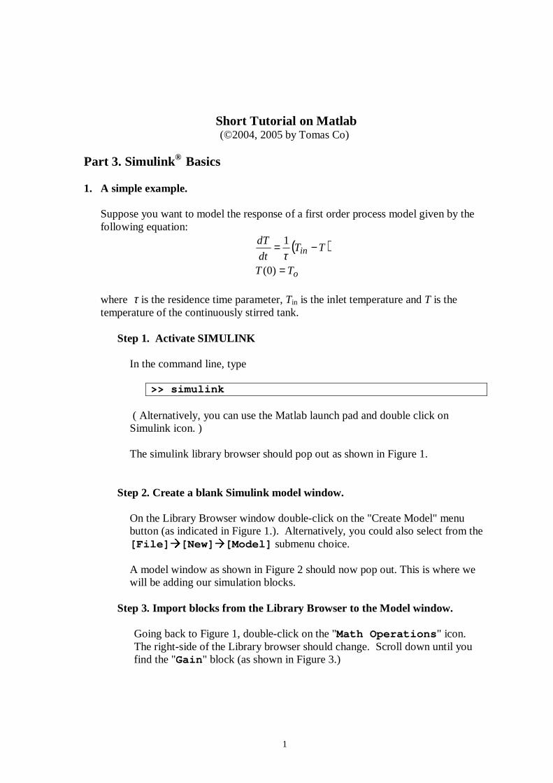
Going back to Figure 1, double-click on the "Math Operations" icon.The right-side of the Library browser should change. Scroll down until youfind the "Gain" block (as shown in Figure 3.)

2

Create ModelButton

MathOperations

Icon

Figure 1.

Figure 2.

3

Gain Block

Figure 3.

Now drag-drop the "Gain" block into the Model window.

Back to the Library browser, on the right side, scroll down further until youfind the "Sum" block and then drag-drop this block into the Model window.

You could move the two blocks (via click-drag) around in the model windowto match what is shown in Figure 4.

Figure 4.

We need three more blocks which are included in other Simulinksubdirectories. First, click on the "Continuous" subdirectory that is on theright side of the Library Browser. This should change the left side of theLibrary Browser window as shown in Figure 5. Select the "Integrator"block and drag-drop it into the Model window.

4

Click on this to change the right side to showthe blocks inside this subdirectory

IntegratorBlock

Figure 5.

Next, in the Library Browser, select the "Sources" subdirectory (left side).On the right side of the Browser, select the "Step" block and drag-drop itinto the Model window.

Finally, in the Library Browser, select the "Sinks" subdirectory (left side).On the right side of the Browser, select the "Scope" block and drag-drop itinto the Model window.

After all these blocks have been imported, the blocks can be moved around tomatch the positions shown in Figure 6.

Figure 6.

5

At this point, it may be instructive to layout the roles and connections amongthese five blocks:

i) The Step block will be used to implement a step change in Tin. ii) The Sum block will be used to take the difference: (Tin-T). Of course, we

need to change the properties of this block to reflect a difference instead ofa sum (which we will do below).

iii) The Gain block will be used to change the difference (Tin-T) by a factor.In our case, this factor will be (1/τ). Thus the output of the Gain blockwill be (1/τ)(Tin-T). In reference to our process model, the calculationsyield the value of the derivative dT/dt.

iv) The Integrator block now takes in the dT/dt signal and outputs thedesired T signal.

v) The Scope block now simply reads in the T signals as a function of timeand plots it in a separate window.

Step 4. Change the properties of the blocks, if needed.

As we mentioned, we need to change the Sum block to obtain a difference. Todo so, double-click the Sum block. A window should pop-up as shown inFigure 7. In the "List of Signs" input box, change the original entry to "|+-".Then click the [OK] button to close this window and go back to the Modelwindow.

Figure 7.

Next, double-click the Step block. A parameter window should pop-up.Match the parameters shown in Figure 8. This means Tin will have a value of20 until the time, t =3. After that, Tin will jump to a value of 30.

6

Figure 8.

Next, double-click the Integrator block. A parameter window should pop-up. In the "Initial value:" input box, change it to 20. This means we are settingTo=20.

Finally, double-click the Gain Block. Another parameter window should pop-out. Suppose we want to use a value of τ = 4 for our time constant. Thismeans the reciprocal, (1/τ)=0.25. Thus, in the parameter window for the Gainblock, change the gain from 1 to 0.25, and click [OK]. ( In the Model window,the value of 0.25 might not show. You can resize the Gain block by clickingon it once, and then dragging the black corners to resize it.)

Step 5. Connect the Blocks.

Method 1: Short cut.To connect the Integrator block and the Scope block, first click on theIntegrator block. Next, CTRL-click on the Scope block. An arrow shouldconnect the two blocks. (Note: the sequence of blocks clicked will determinethe direction of the arrow.)

7

Method 2: Manual.Try connecting the Gain block with the Integrator block. First, move thecursor to the left port of the Gain block until the cursor changes to a crosssymbol. Next, click-drag the cursor to the input port of the Integrator (adotted line should be dragging behind), then release the mouse-click.

Using either method 1 or method 2 to connect the blocks to match Figure 9.

Figure 9.

Next, we need to tap into (i.e. split) the T signal that goes to the Scope block,and feed it back to the Sum block. First, position the cursor somewhere in themiddle portion of the signal line connecting the Integrator block and theScope block as shown in Figure 9. Next, while depressing the CTRL key,click-drag the cursor (which should turn to a cross once you depressed the rightbutton of the mouse) until it is positioned on top of the "minus" port of the Sumblock, then release the buttons. A new split line should appear. (You canresize the signal line by clicking on it once and then dragging the blackcorners.) We now have the final configuration for our model shown in Figure10.

Figure 10.

8

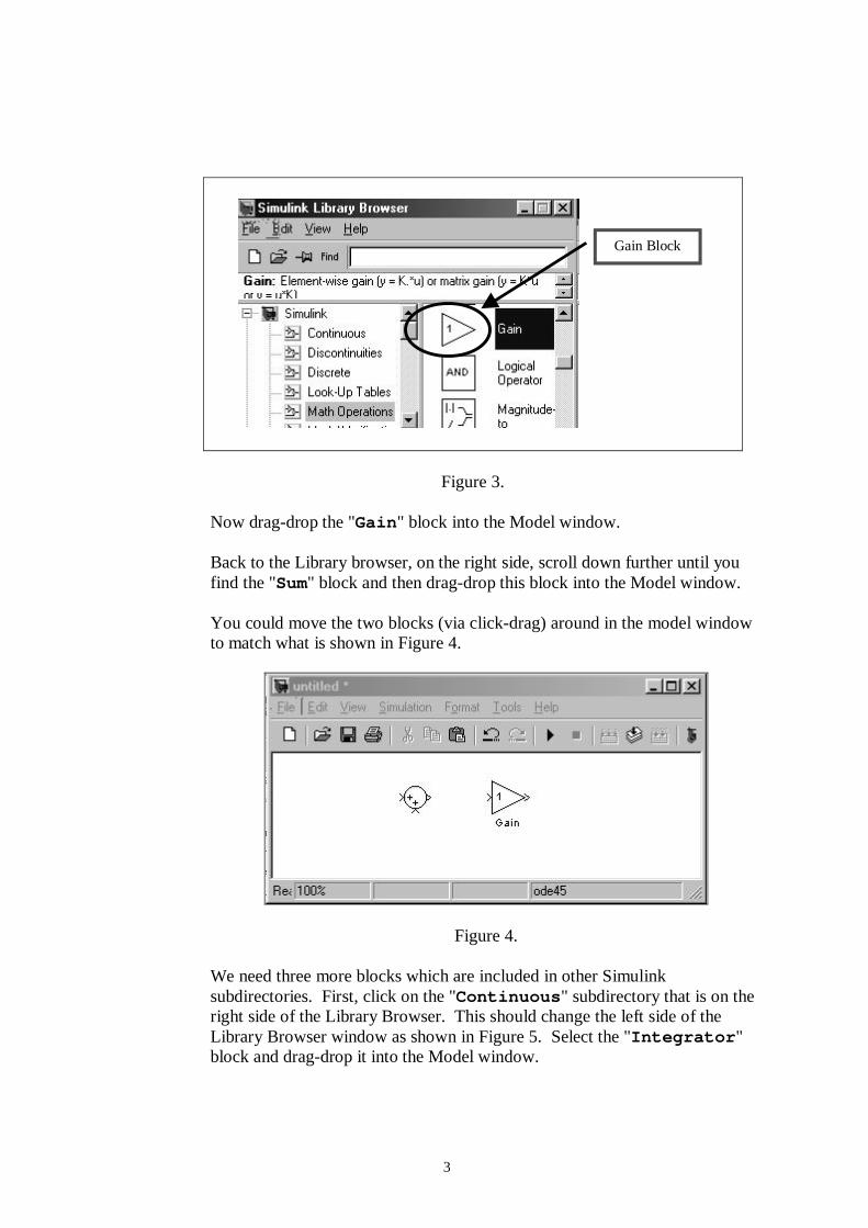
Step 5. Perform the simulation.

We could set simulation parameters by first selecting the submenu item[Simulation] � [Simulation parameters...]

Figure 11.

(for version 7.0, this will be [Configuration parameters...] )

Set the stop time to 20.0 as shown in Figure 12, and then click [OK].

Figure 12.

9

Next, run the simulation by pressing the “Run” button as shown in Figure 13.Alternatively, you can select the [Simulation] � [Start] submenu item(see Figure 11.)

Run Simulation button

Figure 13.

To see the results, double-click the Scope block. A figure with a plot shouldpop out. To see the whole plot, click the “Autoscale” button, as shown inFigure 14.

Figure 14.

10

Step 6. Save the model.

In the Model window, select [File] � [Save As] and save the model. The filewilld be save with a *.mdl extension. (For later purposes, we will save ourmodel system as simple.mdl.)

2. Communication between the Matlab’s Command window/workspace andSimulink’s Model window.

a) Exporting the outputs to the workspace.

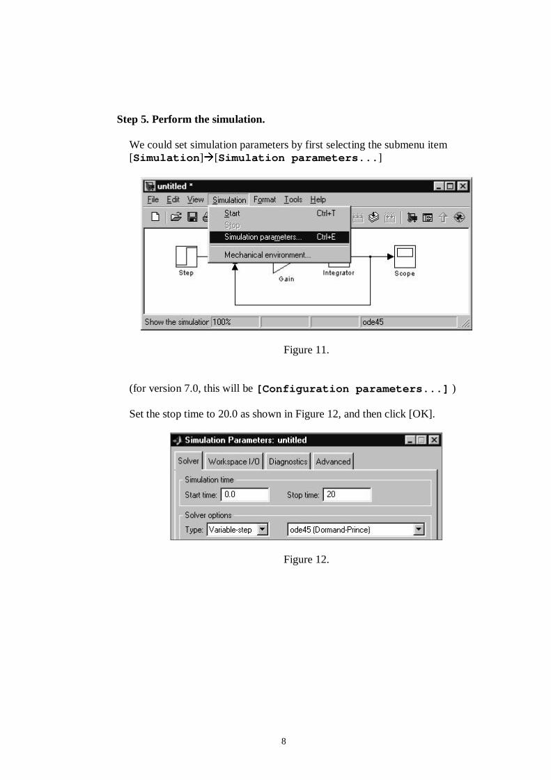
Go to the Simulink Library Browser and select the Sinks subdirectory (on theleft side). From the right side of the browser, drag-drop the [To Worskspace]block into the Model window and drag another split signal to this block as shownin Figure 14.

Figure 14.

Double-click the [To Workspace] block (in Figure 14). A parameter windowshould pop-out. Change the entry in Variable Name to T. Also, change theSave Format selection to “Array” , as shown in Figure 15. Click [OK].

Next, in the Model window, select the [Simulation] � [Simulationparameters...] submenu once more. This time choose the [Workspace I/O]tab. Click on the Time variable and change the name from tout to time asshown in Figure 16. Also, near the bottom of the window, change the Formatto: Array. Click [OK]. (In version 7.0, you need to select [Data import/export])

11

Figure 15.

Figure 16.

12

Start the simulation by clicking the “Run” button. Next, go back to the Matlabcommand window. You should now have the two vectors available in theworkspace: time and T, which you can plot or perform other forms of dataprocessing via Matlab commands.

b) Invoking a Simulink run from Matlab command window.

Sometimes, it may be more eff icient to run the simulation from the commandwindow. For instance, you could change parameters for a range of say 10 valuesusing a script file and then collect the results in a structure or a file for furtherprocessing.

- To read the value of 'Gain' parameter in the Gain block, use the followingcommand:

>> g_svalue=get_param('simple/ Gain','Gain')

Remarks: i) The string, 'simple/Gain' , identifies the Gain block in the

model we called simple (since we saved the model assimple.mdl earlier).

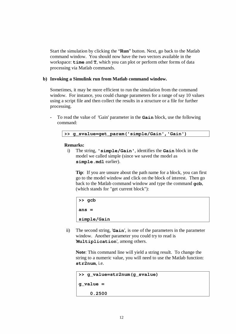
Tip: If you are unsure about the path name for a block, you can firstgo to the model window and click on the block of interest. Then goback to the Matlab command window and type the command gcb ,(which stands for "get current block"):

>> gcb

ans =

simple/Gain

ii) The second string, 'Gai n ', is one of the parameters in the parameterwindow. Another parameter you could try to read is'Multiplicatio n ', among others.

Note: This command line wil l yield a string result. To change thestring to a numeric value, you will need to use the Matlab function:str2num , i.e.

>> g_value=str2num( g_svalue)

g_value =

0.2500

13

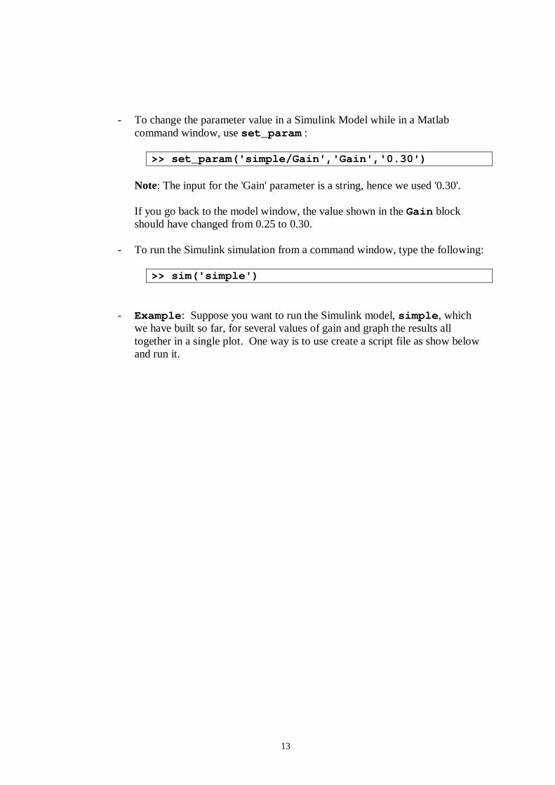
- To change the parameter value in a Simulink Model while in a Matlabcommand window, use set_para m :

>> set _param('simple/Gain','Gain','0.30')

Note: The input for the 'Gain' parameter is a string, hence we used '0.30'.

If you go back to the model window, the value shown in the Gain blockshould have changed from 0.25 to 0.30.

- To run the Simulink simulation from a command window, type the following:

>> sim('simple')

- Example : Suppose you want to run the Simulink model, simple , whichwe have built so far, for several values of gain and graph the results alltogether in a single plot. One way is to use create a script file as show belowand run it.

14

%% Script file for running the Simulink model 'simple'% for different values of gain

% ( c) 2004 Tom Co% @ Michigan Technological Univesity

open _system('simple')

% Initializations% =============== tagCollect =[] ; timeCollect =[] ; TCollect =[ ] ; plotcolors =' bgcmkbgcmkbgcmk' ; nvals = 0 ;

% Calculations% ============for gval=0.2:0.2:1.0 nvals = nvals + 1 ; gvalStr = num2str(gval,3) ; set _param('simple/ Gain','Gain',gvalStr) ; sim('simple') ; timeCollect = [ timeCollect, time] ; TCollect = [ TCollect, T ] ; tag = ['Gain = ', gvalStr] ; tagCollect = [ tagCollect,{tag}] ;

end

% Plotting% ======== hold off for i=1:nvals plot( timeCollect(:, i), TCollect(:, i), plotcolors( i)); hold on end hold off

legend( tagCollect) ;xlabel('Time ( mins)') ;ylabel('Temperature (^ oF)') ;

15

Remarks:

i) We included a line :

open _system('simple')

This is to make sure the Model is open prior to the use of commandsset_param and sim . (If the model, simple , is already open, it will not doanything.)

ii) The variable plotcolors is a string array that would indicate the colorsused for plotting. For example, 'bc g ' will mean the sequence black, cyan,green.

iii ) tagCollect is a cell array, so be careful to use the curly brackets as writtenin the script. We use a cell array because this is what is required by thecommand legend .

iv) Note the use of commands, hold on and hold off to allow the plotcommand not to erase previous plots.

v) Since when using set_param, the gain value should be a string, we need toconvert the numeric value of gval to a string as follows:

gvalStr = num2str(gval,3) ;

where 3 signifies the string wil l show three significant figures.