9/29/16

1

CS 457Networking and the Internet

Fall 2016

Shortest-Path Problem • Given: network topology with link costs

– c(x,y): link cost from node x to node y– Infinity if x and y are not direct neighbors

• Compute: least-cost paths to all nodes– From a given source u to all other nodes– p(v): predecessor node along path from source to v

32

2

1

14

1

4

5

3

u

v

p(v)

Dijkstra’s Shortest-Path Algorithm

• Iterative algorithm– After k iterations, know least-cost path to k nodes

• S: nodes whose least-cost path definitively known– Initially, S = {u} where u is the source node– Add one node to S in each iteration

• D(v): current cost of path from source to node v– Initially, D(v) = c(u,v) for all nodes v adjacent to u– … and D(v) = ∞ for all other nodes v– Continually update D(v) as shorter paths are learned

9/29/16

2

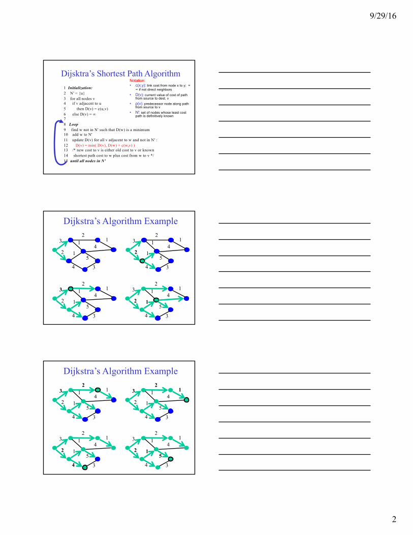
Dijsktra’s Shortest Path Algorithm1 Initialization:2 N' = {u} 3 for all nodes v 4 if v adjacent to u 5 then D(v) = c(u,v) 6 else D(v) = ∞ 7 8 Loop9 find w not in N' such that D(w) is a minimum 10 add w to N' 11 update D(v) for all v adjacent to w and not in N' : 12 D(v) = min( D(v), D(w) + c(w,v) ) 13 /* new cost to v is either old cost to v or known 14 shortest path cost to w plus cost from w to v */ 15 until all nodes in N'

Notation:• c(x,y): link cost from node x to y; =

∞ if not direct neighbors• D(v): current value of cost of path

from source to dest. v• p(v): predecessor node along path

from source to v• N': set of nodes whose least cost

path is definitively known

Dijkstra’s Algorithm Example

32

2

1

14

1

4

5

3

32

2

1

14

1

4

5

3

32

2

1

14

1

4

5

3

32

2

1

14

1

4

5

3

Dijkstra’s Algorithm Example

32

2

1

14

1

4

5

3

32

2

1

14

1

4

5

3

32

2

1

14

1

4

5

3

32

2

1

14

1

4

5

3

9/29/16

3

Shortest-Path Tree• Shortest-path tree

from u• Forwarding table

at u3

2

2

1

14

1

4

5

3

u

v

w

x

y

z

s

t

v (u,v)w (u,w)x (u,w)y (u,v)z (u,v)

link

s (u,w)t (u,w)

Dijkstra’s Algorithm LimitationsAlgorithm complexity: n nodes• each iteration: need to check all nodes, w, not in N• n(n+1)/2 comparisons: O(n2)• more efficient implementations possible: O(mlogn)Oscillations possible when link costs change:• e.g., link cost = amount of carried traffic

AD

C

B1 1+e

e0

e1 1

0 0A

D

C

B2+e 0

001+e 1

AD

C

B0 2+e

1+e10 0

AD

C

B2+e 0

e01+e 1

initially … recomputerouting

… recompute … recompute

Link-State Routing• Each router keeps track of its incident links

– Whether the link is up or down– The cost on the link

• Each router broadcasts the link state– To give every router a complete view of the graph

• Each router runs Dijkstra’s algorithm– To compute the shortest paths– … and construct the forwarding table

• Example protocols– Open Shortest Path First (OSPF)– Intermediate System – Intermediate System (IS-IS)

9/29/16

4

Detecting Topology Changes• Beaconing

– Periodic “hello” messages in both directions– Detect a failure after a few missed “hellos”

• Performance trade-offs– Detection speed– Overhead on link bandwidth and CPU– Likelihood of false detection

“hello”

Broadcasting the Link State• Flooding

– Node sends link-state information out its links– And then the next node sends out all of its links– … except the one where the information arrived

X A

C B D

(a)

X A

C B D

(b)

X A

C B D

(c)

X A

C B D

(d)

Broadcasting the Link State• Reliable flooding

– Ensure all nodes receive link-state information– … and that they use the latest version

• Challenges– Packet loss– Out-of-order arrival

• Solutions– Acknowledgments and retransmissions– Sequence numbers– Time-to-live for each packet

9/29/16

5

When to Initiate Flooding• Topology change

– Link or node failure– Link or node recovery

• Configuration change– Link cost change

• Periodically– Refresh the link-state information– Typically (say) 30 minutes– Corrects for possible corruption of the data

Convergence• Getting consistent routing information to all nodes

– E.g., all nodes having the same link-state database• Consistent forwarding after convergence

– All nodes have the same link-state database– All nodes forward packets on shortest paths– The next router on the path forwards to the next hop

32

2

1

14

1

4

5

3

Transient Disruptions• Detection delay

– A node does not detect a failed link immediately

– … and forwards data packets into a “blackhole”– Depends on timeout for detecting lost hellos

32

2

1

14

1

4

5

3

9/29/16

6

Transient Disruptions• Inconsistent link-state database

– Some routers know about failure before others– The shortest paths are no longer consistent– Can cause transient forwarding loops

32

2

1

14

1

4

5

3

32

2

1

14

1

4 3

Convergence Delay• Sources of convergence delay

– Detection latency– Flooding of link-state information– Shortest-path computation– Creating the forwarding table

• Performance during convergence period– Lost packets due to blackholes and TTL expiry– Looping packets consuming resources– Out-of-order packets reaching the destination

• Very bad for VoIP, online gaming, and video

Reducing Convergence Delay• Faster detection

– Smaller hello timers– Link-layer technologies that can detect failures

• Faster flooding– Flooding immediately– Sending link-state packets with high-priority

• Faster computation– Faster processors on the routers– Incremental Dijkstra algorithm

• Faster forwarding-table update– Data structures supporting incremental updates

9/29/16

7

Comparison of LS and DV algorithms

Message complexity• LS: with n nodes, E links,

O(nE) messages sent • DV: exchange between

neighbors only– Convergence time varies

Speed of Convergence• LS: O(n2) algorithm

requires O(nE) messages• DV: convergence time

varies– May be routing loops– Count-to-infinity

problem

Robustness: what happens if router malfunctions?

LS:– Node can advertise

incorrect link cost– Each node computes only

its own table

DV:– DV node can advertise

incorrect path cost– Each node’s table used by

others (error propagates)

Summary• Routing is a distributed algorithm

– React to changes in the topology– Compute the shortest paths

• Two main shortest-path algorithms– Dijkstra à link-state routing (e.g., OSPF and IS-IS)– Bellman-Ford à distance vector routing (e.g., RIP)

• Convergence process– Changing from one topology to another– Transient periods of inconsistency across routers

Routing in Practice

9/29/16

8

RIP (Routing Information Protocol)

• Distance vector algorithm• Included in BSD-UNIX Distribution in 1982• Distance metric: # of hops (max = 15 hops)• Distance vectors: exchanged among neighbors every 30 sec

via Response Message (also called advertisement)• Each advertisement: list of up to 25 destination nets

RIP: Example

Destination Network Next Router Num. of hops to dest.w A 2y B 2z B 7x -- 1…. …. ....

w x y

z

A

C

D B

Routing table in D

RIP: Example

Destination Network Next Router Num. of hops to dest.w A 2y B 2z B A 7 5x -- 1…. …. ....

Routing table in D

w x y

z

A

C

D B

Dest Next hopsw - -x - -z C 4…. … ...

Advertisementfrom A to D

9/29/16

9

RIP: Link Failure and Recovery

If no advertisement heard after 180 sec --> neighbor/link declared dead– routes via neighbor invalidated– new advertisements sent to neighbors– neighbors in turn send out new advertisements (if

tables changed)– link failure info quickly propagates to entire net– poison reverse used to prevent ping-pong loops

(infinite distance = 16 hops)

RIP Table processing

• RIP routing tables managed by application-level process called route-d (daemon)

• advertisements sent in UDP packets, periodically repeated

routed routed

Transport(UDP)Network(IP)LinkPhysical

ForwardingTable

Transport(UDP)

Network(IP)

LinkPhysical

ForwardingTable

RIP Table example (continued)

Router: giroflee.eurocom.fr

❒ Three attached networks (LANs)❒ Router only knows routes to attached LANs❒ Default router used to “go up”❒ Route multicast address: 224.0.0.0❒ Loopback interface (for debugging)

Destination Gateway Flags Ref Use Interface

-------------------- -------------------- ----- ----- ------ ---------

127.0.0.1 127.0.0.1 UH 0 26492 lo0 192.168.2. 192.168.2.5 U 2 13 fa0 193.55.114. 193.55.114.6 U 3 58503 le0

192.168.3. 192.168.3.5 U 2 25 qaa0 224.0.0.0 193.55.114.6 U 3 0 le0 default 193.55.114.129 UG 0 143454

9/29/16

10

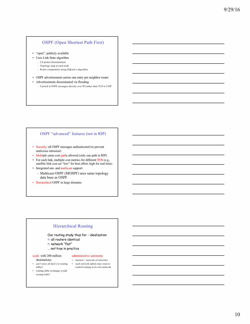
OSPF (Open Shortest Path First)

• “open”: publicly available• Uses Link State algorithm

– LS packet dissemination– Topology map at each node– Route computation using Dijkstra’s algorithm

• OSPF advertisement carries one entry per neighbor router• Advertisements disseminated via flooding

– Carried in OSPF messages directly over IP (rather than TCP or UDP

OSPF “advanced” features (not in RIP)

• Security: all OSPF messages authenticated (to prevent malicious intrusion)

• Multiple same-cost paths allowed (only one path in RIP)• For each link, multiple cost metrics for different TOS (e.g.,

satellite link cost set “low” for best effort; high for real time)• Integrated uni- and multicast support:

– Multicast OSPF (MOSPF) uses same topology data base as OSPF

• Hierarchical OSPF in large domains.

Hierarchical Routing

scale: with 200 million destinations:

• can’t store all dest’s in routing tables!

• routing table exchange would swamp links!

administrative autonomy• internet = network of networks• each network admin may want to

control routing in its own network

Our routing study thus far - idealization ❒ all routers identical❒ network “flat”… not true in practice

9/29/16

11

Hierarchical Routing

• aggregate routers into regions, “autonomous systems” (AS)

• routers in same AS run same routing protocol– “intra-AS” routing protocol– routers in different AS can

run different intra-AS routing protocol

• special routers in AS• run intra-AS routing

protocol with all other routers in AS

• also responsible for routing to destinations outside AS– run inter-AS routing

protocol with other gateway routers

gateway routers

Routing in the Internet

• The Global Internet consists of Autonomous Systems (AS)interconnected with each other:– Stub AS: small corporation: one connection to other AS’s– Multihomed AS: large corporation (no transit): multiple connections to

other AS’s– Transit AS: provider, hooking many AS’s together

• Two-level routing: – Intra-AS: administrator responsible for choice of routing algorithm

within network– Inter-AS: unique standard for inter-AS routing: BGP

Network Layer 4-33

Internet AS HierarchyIntra-AS border (exterior gateway) routers

Inter-AS interior (gateway) routers

9/29/16

12

Intra-AS Routing

• Also known as Interior Gateway Protocols (IGP)• Most common Intra-AS routing protocols:

– RIP: Routing Information Protocol

– OSPF: Open Shortest Path First

– IGRP: Interior Gateway Routing Protocol (Cisco proprietary)

Intra-AS and Inter-AS routing

Host h2

a

b

b

aaC

A

Bd c

A.aA.c

C.bB.a

cb

Hosth1

Intra-AS routingwithin AS A

Inter-ASrouting

between A and B

Intra-AS routingwithin AS B

❒ We’ll examine specific inter-AS and intra-AS Internet routing protocols shortly

Intra-AS and Inter-AS routing

Gateways:• perform inter-AS routing amongst themselves• perform intra-AS routers with other routers in their AS

inter-AS, intra-AS routing in

gateway A.c

network layerlink layerphysical layer

a

b

b

aaC

A

Bd

A.aA.c

C.bB.a

cb

c

9/29/16

13

4-37

Hierarchical OSPF

Hierarchical OSPF

• Two-level hierarchy: local area, backbone.– Link-state advertisements only in area – each nodes has detailed area topology; only know

direction (shortest path) to nets in other areas.• Area border routers: “summarize” distances to nets in own

area, advertise to other Area Border routers.• Backbone routers: run OSPF routing limited to backbone.• Boundary routers: connect to other AS’s.

Network Address Translation

9/29/16

14

NAT: Network Address Translation

10.0.0.1

10.0.0.2

10.0.0.3

10.0.0.4

138.76.29.7

local network(e.g., home network)

10.0.0/24

rest ofInternet

Datagrams with source or destination in this networkhave 10.0.0/24 address for

source, destination (as usual)

All datagrams leaving localnetwork have same single source NAT IP

address: 138.76.29.7,different source port numbers

NAT: Network Address Translation

• Motivation: local network uses just one IP address as far as outside word is concerned:– no need to be allocated range of addresses from ISP:

- just one IP address is used for all devices– can change addresses of devices in local network

without notifying outside world– can change ISP without changing addresses of

devices in local network– devices inside local net not explicitly addressable,

visible by outside world (a security plus).

NAT: Network Address TranslationImplementation: NAT router must:

– outgoing datagrams: replace (source IP address, port #) of every outgoing datagram to (NAT IP address, new port #)

. . . remote clients/servers will respond using (NAT IP address, new port #) as destination addr.

– remember (in NAT translation table) every (source IP address, port #) to (NAT IP address, new port #) translation pair

– incoming datagrams: replace (NAT IP address, new port #) in dest fields of every incoming datagram with corresponding (source IP address, port #) stored in NAT table

9/29/16

15

NAT: Network Address Translation

10.0.0.1

10.0.0.2

10.0.0.3

S: 10.0.0.1, 3345D: 128.119.40.186, 80

110.0.0.4

138.76.29.7

1: host 10.0.0.1 sends datagram to 128.119.40, 80

NAT translation tableWAN side addr LAN side addr

138.76.29.7, 5001 10.0.0.1, 3345…… ……

S: 128.119.40.186, 80 D: 10.0.0.1, 3345 4

S: 138.76.29.7, 5001D: 128.119.40.186, 802

2: NAT routerchanges datagramsource addr from10.0.0.1, 3345 to138.76.29.7, 5001,updates table

S: 128.119.40.186, 80 D: 138.76.29.7, 5001 3

3: Reply arrivesdest. address:138.76.29.7, 5001

4: NAT routerchanges datagramdest addr from138.76.29.7, 5001 to 10.0.0.1, 3345

NAT: Network Address Translation

• 16-bit port-number field: – 60,000 simultaneous connections with a single

LAN-side address!• NAT is controversial:

– routers should only process up to layer 3– violates end-to-end argument

• NAT possibility must be taken into account by app designers, eg, P2P applications

– address shortage should instead be solved by IPv6