Shortfall-Probability-Optimized Portfolios

in the Case of Riskless Borrowing and Lending

Jochen V. ~ a d u f f Swiss Institute of Banking and Finance

University of St. Gallen Merkurstrasse 1

CH-9000 St. Gallen Switzerland

Telephone: +41/ 711 223 81 03 Fax: +41/ 711 223 65 63

E-Mail: jochen.kaduff@sbf.unisg.ch

Internet: http:llwww.unisg.cWsbE/jkaduff.htrn

Abstract This paper analyses different types of shortfall-probability-based diagrams of efficient fron- tiers and compares them with each other in terms of their advantages and disadvantages. Ex- panding the existing literature, the alternative concepts are then generalized for the case of riskless borrowing and lending. In addition, a new type of diagramm is developed, which is able to overcome the shortcomings of existing approaches. A scenario with assets having normally distributed returns is used throughout to illustrate the mathematical analysis. Furthermore, two methods of solving the portfolio selection problem under shortfall risk for the case of arbitrary return distributions are presented.

Keywords Portfolio Optimization, Shortfall Risk, Efficient Frontier, Lower Partial Moment

1. Introduction

It is well known, that under particular assumptions refemng to the shape of asset return distri-

butions, portfolio optimization based on shortfall probabilities according to ROY (1952), leads

to portfolios, which are positioned on the classical Efficient Frontier in the Mean-Variance-

World of MARKOWITZ (1952).' This is especially true in the case of normally distributed re-

turns. Therefore, a section of the p-a-Efficient-Frontier is also efficient in a Mean-Shorrfall-

Probability-World. To take not only analytically but also graphically account of this fact, se-

veral modified representations of the classical Efficient Frontier have been proposed in the

literature. These diagrams may be used by institutional investment committees as well as in

consulting the private banker's client and lead to a better understanding of the shortfall risk

concept, in general. Moreover, performance results can be communicated ex post using these

graphics.

This paper has three main goals: First of all, the most important, already known types of gra-

phical representations are discussed and compared which each other in terms of their advanta-

ges and di~advanta~es.~ Secondly, expanding the existing literatur, the different concepts are

generalized for the (more practical) case of riskless lending and borrowing. Thirdly, a new

type of diagramrn is developed, which is able to overcome the massive shortcomings of the

existing approaches.

The paper is structured as follows: At first, the conventional approaches are explained analyti-

cally and graphically in detail. This is the so-called Mean-LPMo-Effient-Frontier in the se-

cond section, the Efficient Shortfall Frontier in the third section and the L-Efficient-Frontier

in the fourth section. Two illustrative scenarios, one for the sole risky portfolio selection and

one for the possibility of investing in a riskless asset, may help to understand the different

concepts. In the fifth section a new type of diagram, the Efficient Shortfall Surface is introdu-

ced and explained. Whereas for the first five sections the existence of normally distributed

returns is assumed, in the sixth section the consequences of a relaxation of this assumption are

discussed. Two different methods of solving the generalized portfolio optimization problem

under shhrtfall risk are shown. The final appendix contains the data, which are used for the

scenarios.

2. The Mean-LPm-Efficient-Frontier

The first type of shortfall-probabitlity-based representation of portfolios presented here is the

so-called Mean-~~M~~flcient-~rontie? by HARLOW (1991), who positions all feasible port-

folios in a ~ean-shortfall-~robabilit~-~orld~ and derives a corresponding efficient frontier

there. To illustrate the approach, consider a portfolio with a normally distributed return

R-N(j~,o). Specifying a target return t', the probability p(t') of this portfolio of returning less

than this threshold is

Substituting x E 0.2 + p, which represents the transition to a random variable Z-N(O,l), equa-

tion (1) can be modified to

Together with corresponding expected returns all feasible portfolios can be positioned now

in the p-p(i)-~orld. HARLOW (1991) introduced the name Mean-LPMo-EfJiccient-Frontier for

the resulting efficient frontier.' Analytically this alternative efficient frontier can be derived by

substituting the equation of the classical Mean-Variance Efficient ~rontier~.'

into the equation of the shortfall probability (2):

Equation (4) shows for all portfolios positioned on the Markowitz Efficient Frontier the rela-

tionship between their shortfall probability p(t') and their expected return p, given the fixed

target return i. Figure 1 displays the relationship

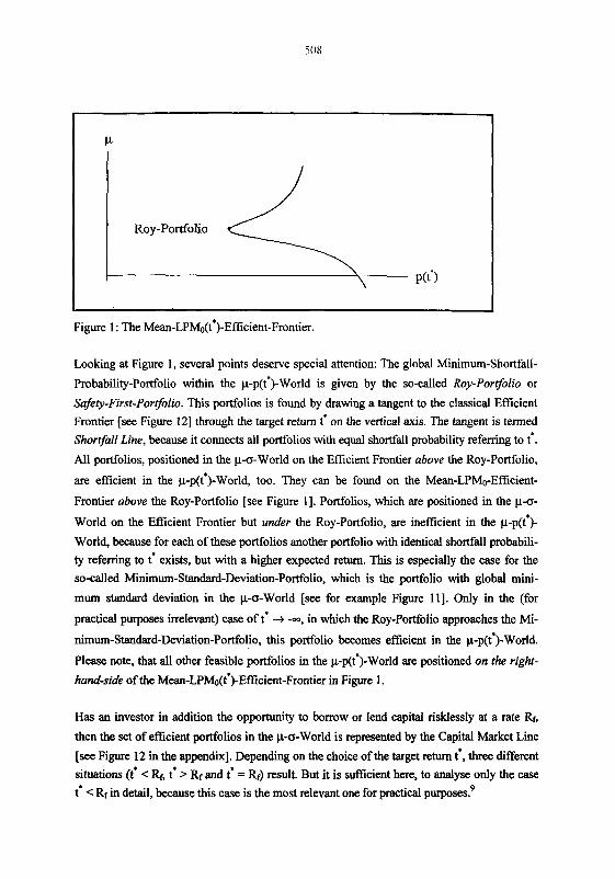
Figure 1 : The ~ean-LPMO({)-~fficient-~rontier.

Looking at Figure 1, several points deserve special attention: The global Minimum-Shortfall-

Probability-Portfolio within the p-p(t')-world is given by the so-called Roy-Portfolio or

Safety-First-Portfolio. This portfolios is found by drawing a tangent to the classical Efficient Frontier [see Figure 121 through the target return t' on the vertical axis. The tangent is termed Shortfall Line, because it connects all portfolios with equal shortfall probability referring to t'. All portfolios, positioned in the y-o-World on the Efficient Frontier above the Roy-Portfolio,

are efficient in the p-p(t')-world, too. They can be found on the Mean-LPMo-Efficient-

Frontier above the Roy-Portfolio [see Figure 11. Portfolios, which are positioned in the pa-

World on the Efficient Frontier but under the Roy-Portfolio, are inefficient in the pp(t')-

World, because for each of these portfolios another portfolio with identical shortfall probabili- ty referring to t' exists, but with a higher expected return. This is especially the case for the so-called Minimum-Standard-Deviation-Portfolio, which is the portfolio with global mini-

mum standard deviation in the p-o-World [see for example Figure 111. Only in the (for

practical purposes irrelevant) case of to + --, in which the Roy-Portfolio approaches the Mi-

nimum-Standard-Deviation-Portfolio, this portfolio becomes efficient in the p-p(t')-~orld.

Please note, that all other feasible portfolios in the pP(t')-world are positioned on the right-

hand-side of the ~ean-LP&(<)-~fficient-~rontier in Figure 1.

Has an investor in addition the opportunity to borrow or lend capital risklessly at a rate Rf,

then the set of efficient portfolios in the p-a-World is represented by the Capital Market Line

[see Figure 12 in the appendix]. Depending on the choice of the target return i, three different situations (t' < Rr, t' > Rf and t' = Rf) result. But it is sufficient here, to analyse only the case

t' < Rf in detail, because this case is the most relevant one for practical purposes?

Analytically, the relationship between expected return and shortfall probability of all Capital

Market Line portfolios can be derived by substituting the equation of the Capital Market Li-

ne''

in the equation

for the slope of the Shortfall Line. Therewith, the negative slopes of the corresponding, now

parameterisized Shortfall Lines result in

S = (p - t*) . (a - Rf . (2 b - cRf))

( p - ~ f ) . J c . ~ f ~ - 2 b ~ f + a

Substituting (7) in (2)" delivers the sought-after relationship

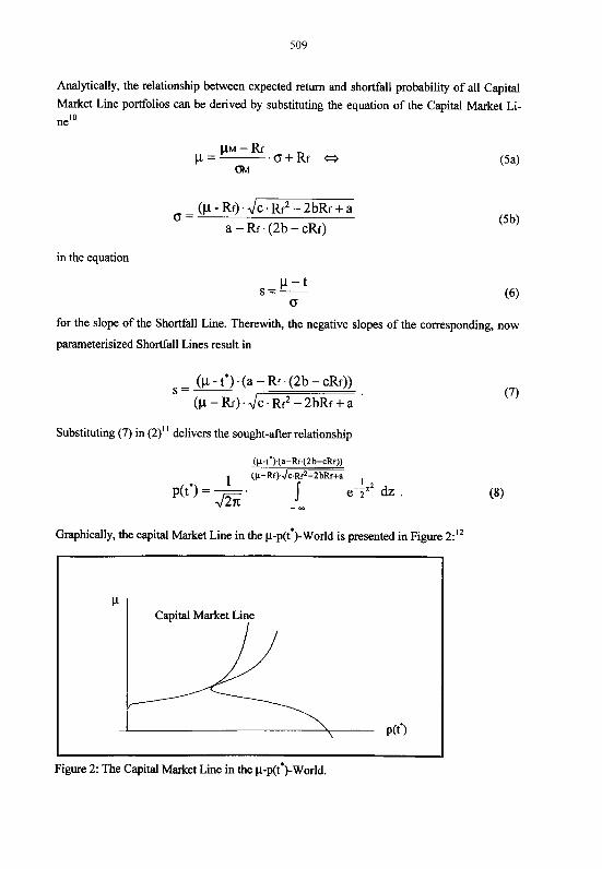
Graphically, the capital Market Line in the pp(t')-world is presented in Figure 2:12

Capital Market Line

Figure 2: The Capital Market Line in the pp(tW)-world.

Two points in Figure 2 are worth noting: Firstly, because of the form of equation (S), the

Capital Market Line in the pp(t')-World is not a straight line, as one might expect from the

classical ~ean-variance-World." But, as expected, the Capital Market Line is tangent to the

Mean-LPMo-Efficient-Frontier, with the Market Portfolio as tangent point, as this is the case

in the po-world.l4

The approach of HARLOW (1991) described so far, has a significant disadvantage: In order to

derive a ~ean-LPMO(<)-~fficient-~rontier, a fured target return i must specified in advance.

This requires, that the investor using Harlow's methodology must be able to specify a single,

most relevant threshold for himself. But in practice, ofien the opposite may be observed: At

the beginning of the asset allocation process, most investorsI5 do not know what is a suitable

target for them and therefore want to consider several or even better all feasible alternatives,

first.I6 To implement such a procedure within the framework of HARLOW (1991), for each

possible target return a separate efficient frontier would have to be calculated and plotted.

Subsequently, all the resulting curves, which can not be drawn in one diagram, must be com-

pared with each other.

3. The Efficient Shortfall Frontier

Is the investor unsure about the suitable target return he should employ, he alternatively can

position all Safety-First-Portfolios in a ~hreshold-Shorlfall-probability-~orld". In this world,

for each feasible target return t the corresponding minimal shortfall probability p(t), which can

be achieved, is displayed. The resulting eficient frontier is termed Eficient Shorlfall Fron-

tier.18 We firstly analyse the situation where there is no riskless asset. Here, the minimal short-

fall probability which can be achieved, can be derived analytically by using the equation of a

tangent

to the Mean-Variance Efficient Frontier in point (crp,pp). Please note, that the Mean-Variance

Efficient Frontier is a hyperbola.I9 Now, for each point (crp,pp) on the efficient section of the

hyperbola, intersection and slope of the corresponding tangent have to be calculated. The in-

tersection equals the target return t, and with the slope of the tangent, the shortfall probability

p(t) can be derived. Substituting these results in (2), the sought-after functional relationship

between target return t and corresponding minimal shortfall probability p(t) is:

Please note also, that in equation (10) the restriction, that only target returns strictly below the

expected return of the Minimurn-Standard-Deviation-Portfolio are allowed, have to be x observed.20 The following Figure 3 represents equation (10) graphically, using the example

from the appendix as underlying data:

In addition, Figure 3 illustrates the situation for t + --. In this case p(t) asymptotically ap-

proaches zero, as it also may be seen analytically fiom (10). Interpreted economically this me-

ans, that an investor is able to meet his decreasing target return with increasing probability.

Graphical correspondence of the process t + -- is the shift of the intercept of the Shortfall

Line in the per-World downwards. In the limiting case, the Shortfall Line equals the vertical

axis. Note also, that the set of all feasible po&folios in Figure 3 is positioned above the Efi-

cient Shortfall Frontier.

The concept of the Efficient Shortfall Frontier can also be generalized for the case of borro- wing and lending risklessly at rate Rf. As it is well known, in this situation the Capital Market

Line represents all efficient portfolios in the p-o-World. Again, three cases have to be consi-

dered: t < Rf, t = Rf and t > Rf. For the case of t > Rf, no Safety-First-Portfolio exist^.^' There-

fore, no Eficient Shortfall Frontier can be generated. The two cases t < Rf and t = Rf can be

analysed together, but a refined distinction of the term ,,target achievement" is in order now: Either the investor interprets risk only as the strict underperformance of the target in the sense of R < t or he wants to outperform the target strictly. The latter can be represented mathemati-

cally by the formulation R 5 t for the shortfall risk. Of course, this refined distinction has just

to be done, if there are discontinous distributions under consideration, because the value of an

integral stays unchanged, if only a single point within the integration interval1 is changed.= Therfore, the generalization for the case of riskless lending and borrowing with a discrete

(because deterministic) distribution, forces the above distinction. Figure 4 displays the situati- on, in which the investor interprets risk only as strict underperformance of the specified target

return:

-

:igure 4: The Efficient Shortfall Frontier with riskless borrowing and lending and strict un-

derperformance of the target return as interpretation of risk.

In this situation, the portfolio invested completely in the riskless asset generates the unambi- gous Safety-First-Portfolio. The shortfall probability of this portfolio, interpreted in the

described manner, is for all t < Rf zero. Geometrically, this means that each point on the Effi-

cient Shortfall Frontier, which is given by a right side enclosed, horizontal half-straight-lime in

Figure 4, represents the same portfolio: complete investment in the riskless asset.

If, on the opposite the investor is interested in strict outperformance of the target, the Efficient Shortfall Frontier exhibits a discontinuity: Now, for t = Rf the riskless portfolio has a shortfall probability of 100% and is therefore not safety first anymore. Instead of this portfolio all port-

folios positioned on the Capital Market Line are safety first.= The shortfall probability of the- se portfolios can be calculated using (2), and is

Figure 5 illustrates the situation:

Rf--IIM A PN

1

,. - > R, t

Figure 5: The Efficient Shortfall Frontier with riskless borrowing and lending and strict out-

performance of the target return as interpretation of risk.

Again, all points on the now right side opened, horizontal half-straight-line represent the risk- less portfolio. But all Capital Market Line portfolios, except the riskless portfolio, are plotted

This approach shows to those investors, who are still unsure about the target return they should use, all alternatives summarized in one diagram. So in this respect, the Efficient Short-

fall Frontier has a clear advantage compared to Harlods Mean-LPMo-Efficient-Frontier

discussed earlier. But on the other hand, an important disadvantage of this type of graph must be considered: The t-p(t)-diagram does not provide any information about the expected return of the portfolios, which is an absolute essential characteristic of any portfolio. Therefore, this

approach is also not able to meet our aim of representing portfolios in a Mean-Shortfall- Probability-World analogue to the Mean-Variance-World.

4. The L-Effkiient-Frontier

The above discussed type of representation for portfolios in a t-p(t)-World is able to show

shortfall-miminal portfolios for all feasible target returns, but offers no information about the

corresponding expected returns of these portfolios. An improved approach by KADUFF/ SPREMANN (1996), the so-called L-Eflcient-Frontier merges both advantages: Without the

need of specifying a fixed target return, all Safety-First-Portfolios are positioned in the pp(t)-

World. Therefore, the expected return of each portfolio can be directly read from such a dia-

gram. One should notice carefully, that the shortfall probability p(t) displayed here on the ho-

rizontal axis, is calculated for varying target returns, which separates the pp(t)-World strictly

from Harlow's p-p(t')-~orld discussed in the second section of this paper.

Analytically, the functional relationship between expected returns and shortfall probabilities

for varying targets of all Safety-First-Portfolios, can be found by substituting the equation for

the hyperbola tangent

in (6) and (2)24,25:

The following Figure 6 shows this relationship graphically. Again, in order to calculate a con-

crete L-Efficient-Frontier, the scenario from the appendix has been used. Several remarks to

Figure 6 are necessary:

1. For p-+ 5% the L-Efficient-Frontier converges on the vertical axis.26 This equals the li-

miting case t + --. In this situation, only relevant for theoretical considerations, the Mi-

nimum-Standard-Deviation-Portfolio is safety first, with a shortfall probability of zero.

1 2. For p(t) + - . dz the L-EEcient-Frontier converges on infity. In the

p-o-World, this situation is represented by shifting the intersection t of the Shortfall L i e

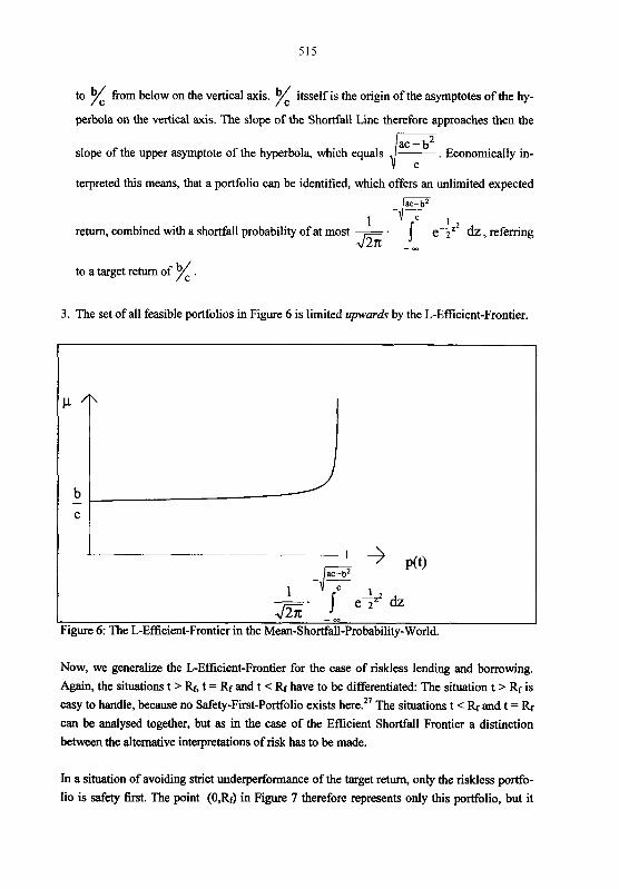
to % from below on the vertical axis. % itsself is the origin of the asymptotes of the hy-

perbola on the vertical axis. The slope of the Shortfall Line therefore approaches then the

slope of the upper asymptote of the hyperbola, which equals d?. - Economically in-

terpreted this means, that a portfolio can be identified, which offers an unlimited expected

-E 1 I

return, combined with a shortfall probability of at most - . --=2 JZi; !- e 2 dz, referring

to a target return of x . 3. The set of all feasible portfolios in Figure 6 is limited upwards by the L-Efficient-Frontier.

1 A

b - C

--CS PO) -E 1 1 -. , r e-5" dz

:igure 6: The L-Efficient-Frontier in the Mean-Shortfall-Probability-World.

Now, we generalize the L-Efficient-Frontier for the case of riskless lending and borrowing. Again, the situations t > Rf, t = Rr and t < Rf have to be differentiated: The situation t > Rf is easy to handle, because no Safety-First-Portfolio exists here.27 The situations t < Rf and t = Rf can be analysed together, but as in the case of the Efficient Shortfall Frontier a distinction between the alternative interpretations of risk has to be made.

In a situation of avoiding strict underperformance of the target return, only the riskless portfo- lio is safety first. The point (0,Rr) in Figure 7 therefore represents only this portfolio, but it

516

should to be stressed that the target return t varies in the background for -- < t 5 Rf. Because

of this, the entire L-Efficient-Frontier is plotted on this single point:

I Figure 7: The L-Efficient-Frontier with riskless lending and borrowing and strict underper-

formance of the target return as interpretation of risk.

With the interpretation of risk as strict outperformance of the target, the diagramm changes

completely [see Figure 81. Now, the resulting curve has a discontinuity. As before, for all t <

Rf, the riskless portfolio is safety first, with a shortfall probability of zero. But if the investor

wants to employ a target return which equals exactly the riskless return, all portfolios on the

Capital Market Line, except the riskless portfolio, are safety first. Their shortfall probability is

given by equation (1 1).

f -. 1 7 e-ii& 1 ... fi - -

Figure 8: The case with riskless lending and borrowing and strict outperformance of the targa

return as interpretation of risk.

Figure 8 deserves an additional explaining remark: In their paper KADUFF/SPREMANN (1996)

denote a curve L-efficient, if it displays for each target t the corresponding Safety-First-

Portfolio with maximum expected return. This distinction was not necessary for the previously

discussed case without riskless lending and borrowing, because the assumption of normally

distributed returns and other usually employed assumptions28 for the optimization problem

guarantee unambiguity. But in the case with riskless lending and borrowing discussed now,

this distinction is necessary. For t = Rf combined with the second interpretation of risk (i. e.

strict outperformance of the target return) no safety-~ean-~fficient-~ortfolio~~ in the sense of

KADUFF/SPREMANN (1996) can be found. In order to keep consistent with the notation in

KADUFF/SPREMANN (1996) the c w e in Figure 8 should not be denoted as L-Efficient-Frontier

in the sense of KADUFF/SPREMANN (1 996).

Summarizing the results, the L-Efficient-Frontier allows the presentation of the expected re-

turns of all Safety-First-Portfolios and their shortfall probabilities referring to all permissible

target returns. But these target returns vary along the L-Efficient-Frontier, without being dis-

played directly in the p-fit)-Wold Ultimately, an investor, who has decided that shortfall

probability is a suitable risk measure for his purposes, has to add not only one but two addi-

tional dimensions to the expected return, that is the shortfall probability and the corresponding

target return, for which the shortfall probability is calculated. The logic consequence is the

extension of the two-dimensional diagrams in a third dimension.

5. The Efficient Shortfall Surface

To proceed in such a manner, in analogy to the p-o-World each feasible portfolio is to be

positioned in a p-t-p(t)-World, a procedure, which can be illustrated graphically very easily.

Again, firstly the case without riskless lending and borrowing is discussed. Of special interest

now are those portfolios, which yield the maximum expected return for a given target return and shortfall probability combination. This criteria of optimization equals the method of

TELSER (1955)", with the difference, that not only one but all feasible t-p(t)-combinations are

considered. Within the pt-p(t)-World, these portfolios generate a surface for which we intro-

duce the name Efficient Shortfall Surface. For the corresponding efficiency property the term ~ean-~horrfall-constraint-~fficienc' will be used.

Analytically, the Mean-Shortfall-Constraint-Efficient Portfolios can be derived by intersecting

the so-called Telser-Lie with the classical Efficient Frontier. The Telser-Lie is the line

identified in the Mean-Variance-World by selecting a target return and a shortfall probability.

The upper intersection point between the Telser-Line and the classical Efficient Frontier iden-

tifies - if existent - the portfolio, which meets the restrictions referring to target return and

shortfall probability and yields the maximum expected return. We will represent this maxi-

mum expected return through ps. Combined with the corresponding standard deviation os,

which can be easily calculated from equation (3) for all portfolios on the Efficient Frontier, ps

is substituted in (2). This results in the equation32:

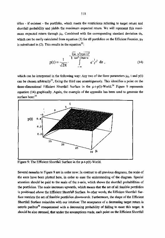
which can be interpreted in the following way: Any two of the three parameters ps, t and p(t)

can be chosen arbitrarilg3, fixing the third one unambiguously. This identifies a point on the

three-dimensional Efficient Shortfall Surface in the p-t-p(t)-~orld?4 Figure 9 represents

equation (14) graphically. Again, the example of the appendix has been used to generate the

surface here?

I t

I Figure 9: The Eficient Shortfall Surface in the p-t-p(t)-World.

Several remarks to Figure 9 are in order now: In contrast to all previous diagrams, the scale of

the axes have been plotted here, in order to ease the understanding of the diagram. Special

attention should be paid to the scale of the z-axis, which shows the shortfall probabilities of the portfolios. The scale increases upwards, which means that the set of all feasible portfolios

is positioned above the Efficient Shortfall Surface. In other words, the Efficient Shortfall Sur-

face restricts the set of feasible portfolios downwards. Furthermore, the shape of the Efficient

Shortfall Surface coincides with our intution: The acceptance of a decreasing target return is

ceteris paribus36 compensated with a decreasing probability of failing to meet this target. It

should be also stressed, that under the assumptions made, each point on the Efficient Shortfall

Surface identifys a portfolio unambiguously [see endnote 341, but this relationship is not in- jective in a mathematical sense. This means, that the same portfolio can be plotted on different points on the Efficient Shortfall Frontier through different t-p(t)-combinations.

Figure 9 can also be employed to visualise the three classical portfolio optimization strategies

based on shortfall probabilities according to ROY (1952), KATAOKA (1963) and TELSER (1955):

1. The Safety-First-Rule of ROY can be illustrated by fitting in a vertical surface, parailel to the surface spanned by the x- and z-axis, runing through the prespecified target return. In-

tersecting this surface with the Efficient Shortfall Surface yields an intersection line in the three-dimensional space. The point on this line with the minimum height referring to the z- axis is the Roy-Portfolio.

2. The ~ataoka-~ortfolio'~ can be identified by intersecting a horizontal surface through the

prespecified shortfall probability with the Efficient Shortfall Surface. Again, an intersection

line in the three-dimensional space results. The point with the maximum y-scale value on this line is the Kataoka-Portfolio.

3. The method of TELSER equals graphically the intersection of a line, generated through the

specification of a target return and corresponding shortfall probabili$8, with the Efficient Shortfall Surface. The resulting intersection point represents the Telser-Portfolio.

In the case of riskless borrowing and lending at rate Rf, the efficient portfolios are represented

in the y-o-World by the Capital Market Line. Dependent on the choice of the intersection

point t ~ ~ l ~ and the slope -ST=,, of the Telser-Line different situations may occur. But relevant for the generation of an Efficient Shortfall Surface for practical purposes are only those situa- tions, in which Telser-Portfolios exist. This is true for ~T,I,, < Rf combined with -sT,I,,, >

PM-Rf . The corresponding expected return ~T,I, can be calculated m

For this area in the p-t-p(t)-World, the following mathematical relationship for Mean-

Shortfall-Constraint-Eficient portfolios holdstO

Again, these portfolios are represented in the three-dimensional space by a surface, to which we will refer as Capital Market Surface. Figure (10) shows equation (16) graphically:

Figure 10: The Capital Market Surface for the case of riskless borrowing and lending.

Several remarks are necessary: Figure 10 is also based on the scenario of the appendix.41 By comparing Figure 9 and Figure 10, one can see that the Capital Market Surface is positioned - as expected - completely below the Eflicient Shortfall Surface. In other words, the Capital Market Surface dominates the Efficent Shortfall Surface. Not that obviously to see but also expected is the fact, that both surfaces are tangent to each other along a c w e . This curve re-

presents all the points in the p-t-p(t)-World, on which the Market Portfolio is plotted. For the-

se points, according to equation (16) the following relationship holds:

Therefore, we now have developed a theorem of separation for the three-dimensional space: Independently of his preferences, each investor structures the risky fraction of his portfolio identically (exactly according to the allocation of risky assets in the Market Portfolio). Depen- dent on his preferences, either capital remains, which is then invested in the riskless asset, or

additional capital is required, which is then borrowed risklessly. The border between borro- wing and lending is given by the curve on the Capital Market Surface, which represents the Market Portfolio. Portfolios, which are positioned on the left-hand-side of this curve contain a long position in the riskless asset. Portfolios, which are positioned on the right-hand-side of the curve contain a short position.

6. Extensions

The previous analysis is, as mentioned, based on the assumption of normally distributed port- folio returns.42 In general, there are two possibilities of treating situations, in which this as-

sumption is violated:

1. The first possibility is to use the inequality of CHEBYSHEV, which requires no information

about the shape of the probability distribututions at all. According to this inequality, the following relationship for the shortfall probability p(t) referring to a target return t holds:

Of course, with this approach no statements about the actual shortfall probabilities of port-

folios can be made, but at least upper bounds for the shortfall probabilities can be calcula-

ted. In this way, all previous derived relationships can be generalized very easily. Also, the

corresponding diagrams may be modified in this manner: In the ~ - ~ ( t ' ) - ~ o r l d the shortfall-

probability-scale on the x-axis is substituted by an upper-boundestimation-scale according to CHEBYSHEV. Therefore, all portfolios are now positioned in a world, which could be de- noted by Mean-Shorrfall-Probability-Bound-World, with a Mean-Shorrfall-Probability- Bound-Eflcient-Frontier. In the t-p(t)-World the y-axis has to be transformed, yielding a

Threshold-Shortfall-Probability-Bound- World, with an Eflcient-Shorybll-Bound-Frontier.

The L-Eficient-Frontier of the pp(t)-World can be transformed into a Generalized-

Disfribution-L-Eflcient-Frontier. The three-dimensional p-t-p(t)-World can be modified to

a Mean-Threshold-Shorrfall-Probability-Bound-World, with an Eflcient-Shortfall-Proba- bility-Bound-Surface.

2. Instead of using no information about the probability distributions of portfolios43, the in- vestor may decide - probably because of empirical investigations - to assume a concrete ty-

pe of not normally distributed asset return. This could be an alternative continuous distri-

bution, for example the lognormal distribution, or a discontinuous one, generated out of the

histogram of historical return realisations. In both cases, no complete equation for the

shortfall probabilities of efficient portfolios can be derived in general, but nevertheless,

shortfall probabilities can be calculated using numerical approximations. The numerical

methods that are available and may be employed can guarantee a sufficient precise analysis

for practical purposes. Because of this, the use of alternative distribution assumptions

admittedly involves extended computing time, but is no problem from a mathematical

point of view.44

Appendix

In order to generate the alternative representations of efficient frontiers displayed in this ar-

ticle, a concrete scenario has been used. To focus attention on the main ideas behind the dia-

grams, it has been refrained from plotting the scale of axes in most of the diagrams. Neverthe-

less, the underlying data of the example will be given here.

Imagine an investor with two investment opportunities with stochastic returns. Mean and

standard deviation of those assets are given by the following table. All data refer to a holding

period of one year and are chosen to have practical relevance:

Table 1: Annual expected returns and standard deviations of the available risky assets.

In addition, the investor knows the covariance matrix between these two assets:

Table 2: Covariance matrix of the risky assets.

The investor can invest any amount of his capital in both assets and is even allowed to sell

them short, if he wants to. Therefore, we have an optimization problem according to BLACK, as it was stated earlier several times. With the data given above, the classical Efficient Fron-

tier of the pa-World according to equation (3) can be generated [see Figure 111. In addition,

for each type of diagramm the case with riskless borrowing and lending is analysed. For the

scenario here, a riskless rate of return of 5% p. a. is assumed. With this rate, the Capital Mar-

ket Line a n be generated, which represents a!l efficient portfolios [see Figure 121.

With the data given, the Minimum-Standard-Deviation-Portfolio has the coordinates (15.27 , 10.31), and the Market Portfolio the coordinates (17.12 , 1 1.68). To generate the Efficient

Frontiers in Figure 11 and 12 the data given so far are sufficient, but in order to calculate the

shortfall probabilities additional information about the shape of the probability distributions is

required. As assumed for the analytical analysis, we use normal-distributions for our dia-

grams. Further, a target return has to be prespecified, corresponding to which the shortfall

524

probabilities are calculated. Here, a target return of 0% has been employed, expressing the idea of nominal capital preservation. Of course, other target returns are possible.

Figure 1 1 : The Efficient Frontier in the p-a-World.

20 -

15 --

I 0 I 1 0

0 5 10 15 20 25 30 35 40

Figure 12: The Capital Market Line in the pa-World.

" Dr. Jochen V. Kaduff, Swiss Institute of Banking and Finance. The author wishes to thank the Gottlieb Daim-

ler- and Karl Benz-Foundation for financial support of his research projekt.

I See for example KADUFF/~PREMANN (1996).

For the case without the possibility of riskless borrowing and lending see also KADUFF (1996a).

The name explains itsself from the fact, that the shortfall probability is exactly the zero-degree Lower Partial

Moment denoted by L P N .

"ereafter, also the term pP([ . ) -~orld is used. The ,,"'-lndex at t indicates, that the target return t, referring to

which the shortfall probability is calculated, has to be fixed.

' HARLOW (1991) analysed ndegree Lower Partial Moments in general. He especially calculated efficient fron-

tiers for fmtdegree and second-degree Lower Partial Moments, but subordinated zero-degree Lower Partial

Moment, because of its inability to yield information about how severe a possible shortfall of the target might be.

This assumes implicitly the presence of an optimization problem according to the Black-Model, i. e. short sel-

ling of all investment opportunities is allowed [see MARKOWITZ (1987)l. But other modellings of the restrictions

in the optimization program can be treated analogously by calculating the shortfall probability for all portfolios

on the referring efficient frontier.

' o is the minimal standard deviation of all portfolios with parametric mean p. V denotes the covariance matrix of

the assets, and v-' the inverse to it. In addition there is a=pTv"p, b=pTvle and c=eTvle, with the unity vector e

of correspondiig dimension.

In order to draw this concrete efficient frontier, a simple but realistic scenario has been used. The underlying

assumptions and data can be found in the appendix.

For the other cases (t' > Rf and t' = k), different scenarios have been analysed, too. Other referring analytical

and graphical results were achieved, which can not all be discussed here. However, some of the results are

presented below.

lo The following modification (5b) of the equation of the Capital Market L i e (5a) is derived by substituting the

relationships

a - b . R r pM=- and

b - c . R r

for the expected return pM and the standard deviation of return aM of the Market Portfolio in (5a). Afterwards,

the equation has to be solved for a.

" Equation (7) specifies the upper integration limit for (2).

l2 Again, in order to generate F i p 2, the scenario described in the appendix has been used.

I' It has to be mentioned, that this is not hue, if i = Rf. In this special case, the Capital Market L i e is represen-

ted by a vertical half-line in the p-p(t')~orld.

l4 Therefore, the theorems of separation for the p - 'jLPM.(Rr)LPM.O-~orld, n = 1, 2, proven in WUFF (1996b)

can be complemented with this case here.

I* This is the case for private as well as institutional investors.

l6 Theoretically, the investor has an unlimited number of alternatives to select his target return ffom. For practical

applications this is of course not hue, but still the number of alternatives can be high.

I' In order to short notation the name I-p(t)-World is going to be used hereafter.

" See JAEGER/RuD~LF/ZIMMERMANN (1995).

l9 This assumes implicitly that an optimization problem according to the Black-Model is used. Other formulati-

ons can be treated analogously . 20 Only this guarantees the existence of tangential points on the eficient section of the hyperbola.

21 For a proof see KADUFF (1996b). 22 The reason is, that for a continous distribution the probability mass of a single point is defined as zero.

Except the riskless portfolio, which is of course also positioned on the Capital Market Line. 24 Again, this assumes implicitly, that an optimization problem according to the Black-Model is used.

2s Under the assumption of normally distributed returns, Safety-First-Portfolios can be found only on the upper

section of the hyperbola. Therefore, p has to satisfy the condition: p > in equation (13). A 26 The term % equals the expected return of the Minimum-Standard-Deviation-Portfolio.

2'See KADUFF (1996b). 2a Arbitrary divisibility of all assets is assumed. In addition, the expected returns are not allowed to be equal for

all assets, and their variances must be finite. Furthermore, it is not possible to represent the random return of any

single asset by a linear combination of the random return of other assets. This ensures the regularity of the cova-

riance matrix, an assumption which guarantees the solvability of the problem. 29 A portfolio is denoted safety mean eficient, if it is safety first referring to a target t and has the maximum ex-

pected retum of all portfolios, which are safety fust referring to this target t [see also Definition 3 in KA-

DUFFISPREMANN (1996)l.

According to TELsER (1955), an investor should specify in advance an individual target return as well as an

acceptable probability of failing to reach that target, and then select from the set of feasible portfolios meeting

both conditions simultaneously the portfolio with the maximum expected return.

" This ternexpresses the fact, that now both risk dimensions, target retwn and corresponding shortfall probabili-

ty are integrated parametrically.

'2 Again, we implicitly assume an optimization problem according to the Black-Model here.

" In choosing ps the restriction ps > x , in choosing t the resixiction t < x and in choosing p(t) the restricti-

on 0 < p(t) < 1 has to be respected.

" The selection of two parameters in the p-o-World is nothing more than the identification of a Shortfall Line,

because a lime can be identified unambiguously by either Wing hvo points (this means choosing ps and t) or

tiximg one point and the slope (this means choosing t and p(t) or ps and p(t)).

l5 For the target return the intervall [-5% ; 8%] and for the expected return the intervall [12% ; 30%] has been

used. This is, because the expected return of the Minimum-Standard-Deviation-Portfolio is 10.32% in our examp-

le, which means that the intervalls for the target return and the expected return must lie below and above, re-

spectively.

l6 Ceteris paribus means here to keep the expected return constantly.

According to KATAOKA (1964) an investor should fmt, in conhast to the approach of ROY (1952), specify an

acceptable shortfall probability, with which the target return, which is to maximise subsequentlly, can be failed to

meet. The portfolio solving this optimization problem is the so-called Kataoka-Portfolio.

38 This line runs parallel to the x-axis in three-dimensional space.

l9 Equation (15) is obtained by equating the formulas of the Telser Line and the Capital Market Line.

Equation (16) is obtained by solving (15) for s,.k and substituting the result as upper integration limit in (2).

" For the target returns, the intervall [-5% ; 4,9%] and for the expected returns the intervall [5.1% ; 30%] have

been employed. The rate for riskless borrowing and lending is 5%.

'' This is the case for all the analytical as well as graphical relationships derived so far.

" ,,No information" refers only to the shape of the probability distributions of the returns. Of course, also the

C H E B Y S H E V - ~ S ~ ~ ~ ~ ~ ~ O ~ S require at least the knowledge of the distribution parameters mean and standard deviati-

on of all assets [see Equation (I8)I. In addition, one has to know the correlations between all asset returns.

In this context the paper of KALNZAGST (1995) should be mentioned. They investigate under which generali-

zed distributions Mean-Variance portfolio optimization and shortfall-risk-based portfolio optimization coincide.

They prove the connection for the wide class of two-parameterdistributions. This class contains besides the

normal-distribution, other in the context of Portfolio Theory commonly used distributions, like the two-point-

distribution, the triangular-distribution and the exponential-distribution.

References

Harlow, W. V.: Asset Pricing in a Downside-Risk Framework, in: Financial Analysts Journal,

September-October, 1991, S.28-40.

Jaeger, Stefan, Markus Rudolf and Heinz Zimmermann: Eflcient Shortfall Frontier, in:

Schmalenbachs Zeitschrift & betriebswirtschaftliche Forschung, Heft 4,1995, S.355-365.

Kaduff, Jochen V.: Shorrfall-Probability-based Diagrams of Eflcient Frontiers, in: Procee-

dings of the 6. International AFIR Colloquium, October 1996a.

Kaduff, Jochen V.: Shorrfall-Risk-basierte Portfolio-Strategien: Grundlagen, Anwendungen,

Algorithmen, Haupt, Bern, 1996b.

Kaduff, Jochen V. and Klaus Spremann: Sicherheit und Diversifhtion bei Shorrfall-Risk, in:

Schmalenbachs Zeitschrift & betriebswirtschaftliche Forschung, Heft 9,1996, S.779-802.

Kalin, Dieter and Rudi Zagst: Porrfolio Optimization under Volatility and Shorrfall Con-

straints, Working Paper, Dept. of Mathematics & Economics, University of Ulm, 1995.

Kataoka, Shinji: A Stochastic Programming Model, in: Econometrica, Vol.3 1, 1963, S. 181 - 196.

Markowitz, Harry M.: Porrfolio Selection, in: Journal of Finance, Vo1.7, 1952, S.77-91.

Markowitz, Harry M.: Mean-Variance Analysis in Portfolio Choice and Capital Markets,

Blackwell, Oxford, 1987.

Roy, Andrew D.: Safety-First and the Holding of Assets, in: Econometrica, Vo1.20, 1952,

S.434-449.

Telser, Lester G.: Safety First and Hedging, in: Review of Economic Studies, Vo1.23, 1955, S.l-16.