GERINI Yannick

Shortwave propagation and communications systems

Shortwave propagation and communications systems:

- types of antennas for shortwave communication systems (3 – 30 MHz), their characteristics

- main modes of propagation and typical coverage areas with respect of 1. antennas used 2. operating frequencies 3. electrical properties of ground 4. ionosphere conditions (depending on solar activity)

- shortwave digital broadcasting (DRM=digital radio mondiale)

I – INTRODUCTION

In this purpose, we will define what we have to do to set up an HF communication, depending on the distance between the two points of the link, and, indeed, some external parameters like attenuation, reflection, ionospheric conditions and even the type of antennas used.

Different type of propagation are usable in the 3 – 30 MHz bandwidth, we will discuss about each of them: frequency usable, coverage, best antennas to use... We will also discuss about the ionospheric condition which is the most important and complicated parameter that avoid skywave propagation.

To conclude, we’ll deal with a new system of communication using the shortwave propagation – the DRM (Digital Radio Mondiale) – which is an improvement of the old AM system.

II – BASIC HF PROPAGATION The HF communication principle is composed by 2 totally different components: the groundwave propagation mode which follows the curvature of the earth and the skywave propagation mode which use the ionosphere layers like a mirror in order to reflect the emitting waves. In this mode, we will see the “near-vertical incidence” HF propagation mode, it’s a special use of the ionosphere propriety to cover areas which can’t be covered by both groundwave and skywave modes. Here we will show how the two modes work. There is also a “line-of-sight” mode which is a transmission between two front to front antennas. A- Groundwave propagation

Ground propagation is usually used for short range AM communications. The propriety of groundwave signal is to follow the curvature of the Earth. At low frequencies (1 kHz to about 3 MHz) the interface between air and the ground acts like an efficient waveguide. This type of propagation depends on different parameters:

- The power of emission: doubling the output power of the signal transmitter will only improve distance range by less than 2%. In order to double the distance of possible reception, we need to multiply by 16 the power of the antenna.

- the position of the antenna over the ground - the environmental noise (man made and atmospheric noise) - The ground conductivity: it depends on the materials present in the sight of the

wave propagation. The atmospheric humidity will guide efficiently the signal. For example, in dry conditions, the signal may only travels a few kilometres (desert < 15Km); in wet conditions, the signal’s range will improve (moist fields ~ 30 Km) and over water the signal will travel about 100 Km to 800 Km. Dense tropical jungles will dramatically decrease propagation distances.

Ground wave intensity decreases with 1/distance² and is diffracted to follow the curvature of the earth. Diffraction increases as frequency decrease and it is also influenced by the imperfect ground conductivity. The reachable distance depends directly of the frequency. We can also use an approximation (flat Earth), which is true if the distance don’t exceed d < 80/(f MHz)1/3. Beyond this value, the signal attenuation will raise quickly. The range for effective transmission decreases with increasing frequency and decreases with decreasing ground conductivity. Low frequencies will provide best range communications. The best usable frequency band is bounded by 4 and 8 MHz. Frequencies lower than 3 MHz are difficult to use because of the level of atmospheric noise especially during the day.

( )

13

1 0

220

tan

2

50

r

r

MHz

b

dp

df

ε ε ωσω

ε σ ωε

− ⎛ ⎞= ⎜ ⎟⎝ ⎠

=+ +

=

Wave attenuation is greater with horizontal polarisation than vertical one, due to the behaviour of both Fresnel reflection coefficients. Advantage: They are relatively unaffected by changing atmospheric conditions. Disadvantages: Requires relatively high transmission power, they are limited to very low, low and medium frequencies which require large antennas, losses on the ground vary considerably with surface material. σ : Type of ground f = 1 MHz f = 10 MHz f = 100 MHz Dry ground (desert) 10-4 10-4 10-4 Fresh ice 10-5 3.10-5 8.10-5 Ground with average conductibility 10-3 10-3 2.10-3 Very moist ground (field) 10-2 10-2 2.10-2 Fresh water (20°C) 3.10-3 3.10-3 5.10-3 Sea water (20°C) 5 5 5

To conclude, in order to use groundwave propagation, it is desirable to use vertical polarisation of the antenna, an AM modulation, and to calculate the proper amplification in order to cover the specified region by taking care of the type of material the signal will encounter. Use: Local Standard Broadcast (AM), Loran C navigation at relatively short ranges. Attenuation: The attenuation of the signal transmitted by the groundwave mode is a function of different parameters like the ground conductivity and the frequency of the signal.

0,62

2 0,3 sin2 0,6 2

pp pA e bp p

−+= −

+ + With:

And the power of the signal received by the transmitter is :

2 222 2

4t t es

reception dirPG AP P A A

dπ= =

with

2

4esA λπ

=

εr Dry ground Ice (-10°C) Ground with

medium conductivity

Very wet ground

Fresh water (20°C)

Sea water (20°C)

εr : ground permittivity

3 3 15 30 80 70

B- Skywave propagation

a) Backgrounds and description

The skywave transmission mode uses the reflection of the ionosphere. Radio waves hit the ionosphere and are bent or refracted depending on the frequency and the angle of the emitting beam. A successful HF transmission using the skywave propagation depends on the conditions of the ionosphere. The ionosphere refers to the upper regions of the atmosphere (90 to 1000 km). This region is highly ionized due to the sun’s ultraviolet radiation. It is composed by different layers because of different frequencies in the sun’s UV spectrum. The lower UV frequency affects the upper ionosphere layer. Ionisation of the atmosphere may also be caused by particles radiation from sunspots, cosmic rays and meteors activity. The ionosphere is a layered region on ionized gas above the earth. The layers of the ionosphere are different during day and night. They act like silver mirrors which reflect or refract the wave depending on its frequency. Each layer may reflect properly (with minimum attenuation) a specific band frequency. The critical frequency is the highest frequency at a certain time and location at which RF energy is reflected back to earth for a near vertical incidence, and it is also the plasma frequency in the layer of the ionosphere. Above this frequency, the wave emitted becomes evanescent and go through the layer (even lost in space).

D-layer: (P = 2 Pa, t = -76°C, electronic density Ne < 105e/m3 composed with polyatomic ions, O3…). It exists only in day time. This layer occupies an area between 50-65 and 80-90 km above the earth. This region of the ionosphere is very absorptive (O3 is the most chemistry compound element present in this region) because of its high collision frequency. The air density in this region is high and the recombination of the ions is very fast, so the ionisation is low. After sunset, this layer disappears, and sometimes in winter it doesn’t appear at all. D is an absorptive layer in HF communications. E-layer: (P = 0.01 Pa, t = -50°C, Ne = 106e/m3 composed with oxygen, nitrogen). This region occupies an area between 90 and 140 Km. It depends directly on the sun’s UV radiation, so the layer is denser directly under the sun exposure and varies with seasons (the sun’s zenith angle changes). This layer disappears gradually after sunset but still lingers at night due to low recombination rates. In summer solstice, some ionized gases appear in the E layer for between few minutes and few hours, with are called “sporadic E” or “Es” phenomenon. E-layer absorbs signals at the lower frequency end of the HF spectrum. F-layer: (P = 0.0001 Pa, t = 1000°C, Ne = 106e/m3 to 1012e/m3 composition: nitrogen in F1, oxygen in F2). This layer may split into two different layers: F1 and F2 but only during day and even under hot summer sun, and by this way, the F layer become less effective than during winter’s days. At night, the F1 layer will rise and merge with the F2 layer. The F1 occupies and area between 140 and 250 Km, and follow the same behaviour as the E layer, that it disappears when the sun disappears below the horizon. The F2 occupies and area between 150 and 300 Km, depending on the day time and the seasons, by night, the layer exists between 150 and 250 Km, during day it reaches 250 to 300 Km above the Earth. The height variation is due to the sun activity (heat and sunspots) and the earth’s magnetic field. During winter’s days, when the F layer don’t split into 2 regions, the wave’s reflection is more efficient especially for frequencies at the high end of the HF spectrum; at night, reflection is interesting for frequencies towards the lower end of the HF spectrum.

The ionosphere is composed by a high density of free electrons (negative) and ions (positive). The charges have important effects on HF transmission:

1. Variations in the electron density (Ne) witch cause waves to bent back to earth in consideration of specific frequency and angle of the emitting antenna.

2. The earth’s magnetic field causes the ionosphere to behave like an anisotropic medium. The polarisation of the emitting wave may change by reflecting on the ionosphere.

HF propagation using ionosphere reflection depends on different parameters such as:

- Latitude: The sun illuminates more the equatorial regions so the ionisation intensity is greater in this region than near the poles. Critical frequency for E-layer and F-layer vary with the sun elevation and the F2-layer varies more with the latitude due to an ionisation variance in the layer inducted by others sources like X-rays, cosmic rays and earth’s magnetic field. The location of emission is also very important. Here are some examples ordered by ascendant difficulty: Temperate regions, especially over water (low values of dispersion and Doppler spread due to the high reflective coefficient of the water) Trans-equatorial (F layer is more diffuse and causes high time dispersion) Auroral ovals (the magnetic field perturbs the signal) Trans-auroral (magnetic storms and solar flares disturbance) Polar cap (Doppler = 10Hz and time dispersion = 1 to 2 ms)

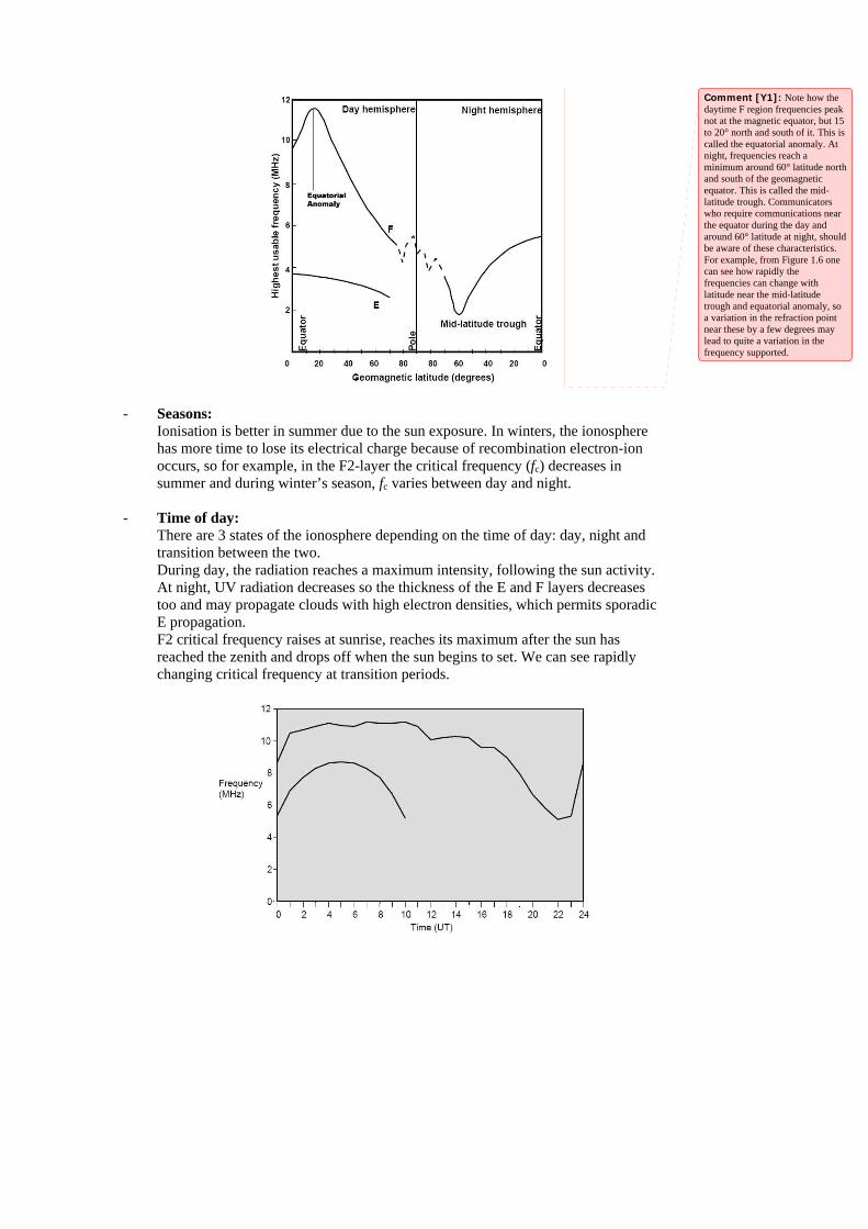
- Seasons: Ionisation is better in summer due to the sun exposure. In winters, the ionosphere has more time to lose its electrical charge because of recombination electron-ion occurs, so for example, in the F2-layer the critical frequency (fc) decreases in summer and during winter’s season, fc varies between day and night.

- Time of day: There are 3 states of the ionosphere depending on the time of day: day, night and transition between the two. During day, the radiation reaches a maximum intensity, following the sun activity. At night, UV radiation decreases so the thickness of the E and F layers decreases too and may propagate clouds with high electron densities, which permits sporadic E propagation. F2 critical frequency raises at sunrise, reaches its maximum after the sun has reached the zenith and drops off when the sun begins to set. We can see rapidly changing critical frequency at transition periods.

Comment [Y1]: Note how the daytime F region frequencies peak not at the magnetic equator, but 15 to 20° north and south of it. This is called the equatorial anomaly. At night, frequencies reach a minimum around 60° latitude north and south of the geomagnetic equator. This is called the mid-latitude trough. Communicators who require communications near the equator during the day and around 60° latitude at night, should be aware of these characteristics. For example, from Figure 1.6 one can see how rapidly the frequencies can change with latitude near the mid-latitude trough and equatorial anomaly, so a variation in the refraction point near these by a few degrees may lead to quite a variation in the frequency supported.

- Cyclical sun variation: Sunspots modify atmospheric behaviour because they have a direct bearing on UV radiation intensity of the sun. They modify the critical frequency and the maximum usable frequency (MUF = higher frequency of use on an oblique incidence path, MUF is greater than critical frequency). During low sunspot activity, MUF < 17 MHz, and during max sunspot, MUF>5O MHz)

- Abnormal propagation conditions: Magnetic storms Sudden ionospheric disturbance Polar blackout Solar flares, which can provoke disturbance even 36 hours after they begun. Flares are huge explosions on the Sun which emit radiation that ionises the D region causing increased absorption of HF waves. Since the D region is present only during the day, only those communication paths which pass through daylight will be affected. The absorption of HF waves travelling via the ionosphere after a flare has occurred is called a short wave fade-out. Affects low frequencies in particular. X-rays, UV radiations, cosmic noise provide heavy HF skywave signal attenuation.

Parameters: to know the critical frequency of each layer and the MUF, we must know the electronic density of the layers and the incidence angle of the emitted beam. In this way,

( )9

secc e

c

f N

MUF f i

=

= This tab contains the MUF and the OWF (optimum working frequency, or “fréquence optimum de travail”: FOT) of the different layers: The OWF is often taken as 85% of the MUF.

Layers D E F1 MUF (MHz) 16 28 16 OWF (MHz) 13.6 23.8 13.6

b) Skywave propagation phenomenon:

Reflections from the emitted beam take place in the E/F1/F2 layers by any of them or

all at once. There are different modes of propagation depending on path length and ionospheric

conditions. A wave can be reflected more than one time (we speak about multiple hops), or trapped between the E and F layers because of a change in the electronic charge, more or less important, in this layer.

When the distance is important, signal from more than one mode can be received. This multi-path propagation causes signal dispersion. It is due to :

• Multiple hop • Multilayer propagation • Low and High angle paths • Ordinary and extraordinary rays from one or more paths

When multiple modes occur, the higher mode suffers greater attenuation because the wave had to travel through the D-layer twice and one more time to reflect on the ground. Wave splitting : A ray entering the ionosphere is splitted into 2 waves due to the Earth’s magnetic field :

- the O (ordinary) wave, less refracted than the other, reflected at a higher altitude, has a lower fc and MUF

- the X (extraordinary) wave. The time dispersion between O and X waves is about 1 to 10 microseconds and the predominant wave is the ordinary one. Mutipath : there is also a problem with constructive or destructive waves when a wave from the first hop strikes a wave from the second and next...

c) Skip zone:

It’s an area of silence located between the outer limit of the groundwave communication and the inner limit of the skywave communication (first hop). This phenomenon can be avoided by a subset of skywave communication called “near vertical incidence”; an antenna emits nearly and the wave is reflected by the F-layer, so the coverage under this incidence angle is about 30 – 800 Km. Skip zones vary in size during the day, with the seasons, and with solar activity. During the day, solar maximum and around the equinoxes, skip zones generally are smaller in area. The ionosphere during these times has increased electron density and so is able to support higher frequencies.

d) Propagation modes : There are many paths by which a sky wave may travel from a transmitter to a receiver.

The mode by a particular layer which requires the least number of hops between the transmitter and receiver is called the first order mode. The mode that requires one extra hop is called the second order mode. For a circuit with a path length of 5000 km, the first order F

mode has two hops (2F), while the second order F mode has three hops (3F). The first order E mode has the same number of hops as the first order F mode. If this results in a hop length of greater than 2050 km, which corresponds to an elevation angle of 0°, then the E mode is not possible. This also applies to the second order E mode. Of course, the E region modes will only be available on daylight circuits.

Simple modes are those propagated by one region, say the F region. IPS predictions are made only for these simple modes, Figure 2.4. More complicated modes consisting of combinations of refractions from the E and F regions, ducting and chordal modes are also possible.

Chordal modes and ducting involve a number of refractions from the ionosphere

without intermediate reflections from the Earth. There is a tendency to think of the regions of the ionosphere as being smooth, however, the ionosphere undulates and moves, with waves passing through it which may affect the refraction of the signal. The ionospheric regions may tilt and when this happens chordal and ducted modes may occur. Ionospheric tilting is more likely near the equatorial anomaly, the mid-latitude trough and in the sunrise and sunset sectors. When these types of modes do occur, signals can be strong since the wave spends less time traversing the D region and being attenuated during ground reflections.

Because of the high electron density of the daytime ionosphere in the vicinity of 15° of

the magnetic equator (near the equatorial anomaly), transequatorial paths can use these enhancements to propagate on higher frequencies. Any tilting of the ionosphere may result in chordal modes, producing good signal strength over long distances. Ducting may result if tilting occurs and the wave becomes trapped between refracting regions of the ionosphere. This is most likely to occur in the equatorial ionosphere, near the auroral zone and mid-latitude trough. Disturbances to the ionosphere, such as travelling ionospheric disturbances, may also account for ducting and chordal mode propagation.

C- Near-vertical incidence (NVI)

It is used to fill the skip zone. The angle of incidence must be very high, near vertical position. High angle of incidence induces a high dispersion more than 10 times as an oblique propagation. We can use NVI propagation only for frequencies between 2 and 10 MHz because above, the atmosphere filters higher frequencies owing the high incidence angle of emission. To perform good transmission in the skip zone, it is useful to minimise ground wave propagation with can interfere with the normal signal. The average circle diameter of coverage area is about 800 miles.

+ Relatively free from fading Simple dipoles work well Low power needed _ Interfere with groundwave propagation Limited bandwidth due to atmospheric absorption Must use two different frequencies because of the difference in the layer between day

and night Antennas must be positioned close to the ground in order to reduce the generation of a

groundwave signal.

D- Line-of-sight (LOS)

It’s direct antenna to antenna transmission. The only thing that must be considered is the atmospheric attenuation and the interferences due to reflective waves from the ground.

The maximum distance between two antennas is set as : 3,57 avec 4 / 3d Kh K= =

Or when the antennas don’t have the same height :

( )1 23,57d Kh Kh= +

III – HF IMPAIRMENTS A – Main components of a radio wave Component Comments Direct wave Free-space propagation, LOS systems Reflected wave Reflection from a passive antenna, ground,

wall, object, ionosphere, etc. Refracted wave Standard, Sub-, and Super-refraction,

ducting, ionized layer refraction (<~100MHz)

Diffracted wave Ground-, mountain-, spherical earth-diffraction (<~5GHz)

Scatter wave Troposcatter wave, precipitation-scatter wave, ionized-layer scatter wave

B – Fading Amplitude and phase of signals fluctuate with reference to time, space and frequency.

1. Interference fading

It’s the most common phenomenon, a mix of two or more signals propagating along different paths. This occurs especially during transition periods and at night.

2. Polarisation fading It’s due to Faraday Rotation. Earth’s magnetic field splits the wave into O and X rays. An originally linear polarised wave becomes an elliptically polarised resultant wave. Its major axis will change it’s direction constantly because of the variation of the electronic density encountered along its propagation path. By this way, the receiving HF antenna will receive every polarisation, vertical to horizontal with a mix of the two, and so, the input level will be bounded by 0 to maximum. Polarisation fading lasts from some millisecond to more than one second.

3. Focusing/defocusing Due to atmospheric irregularities. A signal may be deformed by irregularities in the atmosphere which play like concave or convexe mirrors. Depending on the shape of these irregularities, they can cause periods fading up to some minutes.

4. Absorption fading Caused by solar flares activity. Affects low frequencies and can last from few minutes to about one hour.

Skip fading can be observed around sunrise and sunset particularly, when the operating frequency is close to the MUF, or when the receiving antenna is positioned close to the boundary of the skip zone. At these times of the day, the ionosphere is unstable and the frequency may oscillate above and below the MUF causing the signal to fade in and out. If the receiver site is close to the skip zone boundary, as the ionosphere fluctuates, the skip zone boundary also fluctuates. C – Effects observed in transmission

1. Time dispersion In skywave, it’s due to a multipath propagation and cause amplitude and phase

variation in the signal spectrum. It causes serious and destructive impairments to digital communication signals on HF. By definition, if the delay spread exceed half the time of the period of a signal element (baud), error rate becomes intolerable.

We can struggle this impairment by lowering the baud rate. Multipath and so, time dispersion are correlated with the operating frequency

relative to the MUF. Delay tends to zero if the operating frequency tends to the MUF, it’s because, when we approach the MUF value, we will receive only one signal power component (O).

2. Frequency dispersion (Doppler spread) Generally, frequency dispersion is almost always shown with time dispersion ;

it appears when the signal encounters elemental surfaces of the ionosphere with different velocity vectors. This may have disastrous effects, especially on sensitive systems which require low Doppler spread effects (less than 2Hz).

D – Effects observed in reception

1. Interference The ITV – IFRB is an American organism who assigns frequencies to the users

in order to avoid different HF emitters to interfere each others. They divided the world in three parts, the way to keep transmissions clean.

To make an HF link, we have to find a « clean to interference » frequency, or, if it is impossible, to use frequency which will not interfere each transmission used by both antennas, owing that there are not in the same zone. The amount of interference depends on the power of the emitting antenna.

To achieve our transmission, we can : Find a clean frequency Increase transmitting power to higher the signal/noise ratio Use directional antennas Use antenna nulling (create a silent zone, in the direction of the

interferer, with an electronic directional beam) Use specific frequency preselection on receiver

2. Atmospheric noise Due to thunderstorms (especially in tropical regions), it appears under the

shape of an electrical disturbance transmitted via the ionosphere along huge distances, like the HF transmissions.

As ionosphere attenuates signal and noise, and depending on its behaviour (day and time), atmospheric noise varies with location and time. Local thunderstorms may add a 10dB noise to the normal atmospheric long-range noise. Local thunderstorms add impulse noise to the signal (crashes), and long-distance storms add a rapid and irregular fluctuation (10-20Khz), plus an attenuated wave train oscillation.

Amplitude of lightning disturbance is proportional to 1/f ², this disturbance is propagated in all directions and has an effect on both skywave and groundwave propagations. Atmospheric noise is predominant at low frequencies (<10MHz).

We can define an antenna noise factor :

0 0

n aa

P TfkT b T

= =

0

where : the noise power available from an equivalent loss-free antenna (W)228,6 dBW/Hz : Boltzmann's constant

the effective noise bandwidth (Hz)288 Kthe effective antenna temperature in t

n

a

PkbTT

== −=== he presence of external noise

3. Man-made noise Man-made noise includes ignition noise, neon signs, electrical cables, power

transmission lines and welding machines. This type of noise depends on the technology used by the society and its population. Interference may be intentional, such as jamming, due to propagation conditions or the result of others working on the same frequency.

Man-made noise tends to be vertically polarised, so selecting a horizontally polarised antenna may help in reducing noise. Using a narrower bandwidth, or a directional receiving antenna (with a lobe in the direction of the transmitting source and a null in the direction of the unwanted noise source), will also aid in reducing the effects of noise. Selecting a site with a low noise level and determining the major noise sources are important factors in establishing a successful communications system.

This noise is predominant above 10MHz.

E – Transmission losses

Components :

( ) dBFSL D B ML L L L L= + + + LFSL : free-space loss LD : D-layer absorption LB : ground reflection losses LM : Miscellaneous losses

1. Free-space loss If path distance (A – B) is greater than 1000Km, the great circle distance from A to

B converge to the effective distance deff and we have to use the « normal » distance in the formula, elsewhere we must replace it by deff formula for short-range paths.

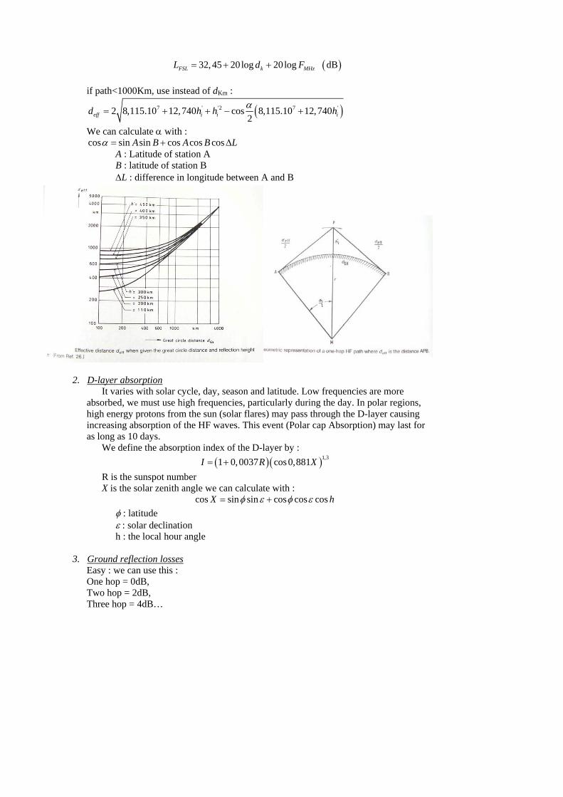
( )32,45 20log 20log dBFSL k MHzL d F= + + if path<1000Km, use instead of dKm :

( )7 ' '2 7 '2 8,115.10 12,740 cos 8,115.10 12,7402eff i i id h h hα

= + + − +

We can calculate α with : cos sin sin cos cos cosA B A B Lα = + Δ A : Latitude of station A

B : latitude of station B ΔL : difference in longitude between A and B

2. D-layer absorption It varies with solar cycle, day, season and latitude. Low frequencies are more

absorbed, we must use high frequencies, particularly during the day. In polar regions, high energy protons from the sun (solar flares) may pass through the D-layer causing increasing absorption of the HF waves. This event (Polar cap Absorption) may last for as long as 10 days.

We define the absorption index of the D-layer by : ( )( )1,31 0,0037 cos 0,881I R X= +

R is the sunspot number X is the solar zenith angle we can calculate with :

cos sin sin cos cos cosX hφ ε φ ε= + φ : latitude ε : solar declination h : the local hour angle

3. Ground reflection losses

Easy : we can use this : One hop = 0dB, Two hop = 2dB, Three hop = 4dB…

4. Miscellaneous When nothing is notified, we can use LM = 7,3dB.

IV - TYPES OF ANTENNAS FOR HF TRANSMISSIONS

A. Recall, propagation modes

Usable frequency

Coverage areas Parameters Characteristics

Ground wave

4 – 8 MHz 15 km (desert) to 800 km (water)

f, ground conductivity, noise, position of antenna, power of emission

Vertical polarisation AM modulation Require large antennas

Sky wave 2 – 30 MHz 1000 – 12000+ Depends on layer used, and number of hop :

hop E F1 F2 1 2000 3400 4000 2 4000 5500 7000 3 7000 9500 12000

Ionosphere (time, season, latitude, solar activity), f, incidence angle

Ionosphere acts like a mirror Hop communication Long range Best frequency difficult to find Use 2 frequencies (day & night) Use a prediction software

LOS 2 – 30 MHz ( )1 23,57d Kh Kh= +

Distance, atmosphere conditions, height of antenna

High power not needed Sensitive to interferences

NVI 2 – 10 MHz ~ 1200 km Ionosphere, incidence angle, f

Simple antennas needed Low power Antennas placed close to the ground

B. Parameters

A certain number of parameters define an antenna :

- Radiation pattern : determine the gain of the antenna owing the angle of emission and so for both horizontal and vertical polarisations.

- Polarisation : the emitted orientation of the wave. It exists horizontal, vertical and elliptic orientation, the last one is used in HF communications.

- Impedance : depends on radiation resistance, reactive storage fields , conductor losses, coupled impedance effects from nearby conductors.

- Gain : it’s defined as G = Max power radiated/ Max reference power radiated. The reference is an antenna which emits the same power in every direction.

- Ground effects : can change impedance of antennas, introduce interference, and allow groundwave propagation.

- Bandwidth : usable frequencies on a system.

C. Type of antennas and characteristics associated

Propagation Groundwave Skywave LOS NVI Type

Whip Tower

Log-periodic Monopole/dipolesYagi Long wire Rhombic V Cone Cage Antenna network

Same as skywave

Dipole/doublets Inverted V/L loops

Characteristics of some antennas :

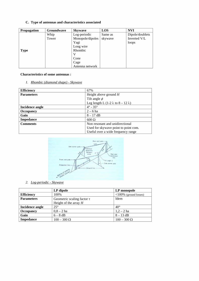
1. Rhombic (diamond shape) - Skywave Efficiency 67% Parameters Height above ground H

Tilt angle φ Leg length L (1-2 λ to 8 – 12 λ)

Incidence angle 4° - 35° Occupancy 2 – 6 ha Gain 8 – 17 dB Impedance 600 Ω Comments Non resonant and unidirectional

Used for skywave point to point com. Useful over a wide frequency range

2. Log-periodic - Skywave

LP dipole LP monopole Efficiency 100% <100% (ground losses) Parameters Geometric scaling factor τ

Height of the array H Idem

Incidence angle 25° 40° Occupancy 0,8 – 2 ha 1,2 – 2 ha Gain 6 – 8 dB 8 – 13 dB Impedance 100 – 300 Ω 100 – 300 Ω

Comments A trapezoidal model exists and have a gain ~16dB

3. Dipoles/doublets – Skywave/NVI Have to be installed 0,1 to 0,25 λ above ground Incidence angle is 30° to 90° Low impedance, no need of a tuner Easy to install If height above the ground decreases, the grain decreases but the noise and the interferences decrease too. Z = 50 Ω

4. Broadband vertical antennas - Skywave Parameters Conic flare a

Conic base diameter Cmax , Cmin Disc-to-cone spacing s

Occupancy 1,2 ha Gain 2 – 5 dB Impedance 50 Ω

5. Yagi - Skywave Parameters Height above ground H (0,25 – 2,5 λ)

Number of elements n Length of elements ln (~0,5 λ) Element spacing d Radius of the elements a (0,3 – 2 λ)

Gain 8 – 18 dB Incidence angle 5° - ? Impedance 50 Ω Comments Difficult to have low take-off angles

Have a small bandwidth

6. Towers - Groundwave Height of the tower determines the gain of this type of antenna. For the lower frequencies of the HF band, the tower may height about 60m. Impedance is about 50 Ω.

7. Horizontal Vee – Skywave/NVI Efficiency 35 – 50 % Parameters Height above ground H

Apex angle α Leg length L Vertical radiation angle Δ

Occupancy 1,2 – 3 ha Height 23m Gain 5 – 9 dB Impedance 500 Ω

8. Inverted V/L - NVI Radiate equally in all directions (even straight up) Must be installed higher than the dipole model Keep the V-angle as shallow as possible otherwise the antenna will receive a lot of noise like distant thunderstorms

V – DIGITAL RADIO MONDIALE

A. History

At the end of XXIst century, era of the digital information, radio looks old fashioned in comparison of digital medias like computers and GSM networks. In September 1996 emerged the D.R.M. agency from a meeting in Paris between international broadcasters and broadcasting equipments manufacturers.

The DRM Consortium formed in 1998 when a small group of pioneering broadcasters and manufacturers joined forces to create a universal, digital system, DRM, for the AM broadcasting bands in HF, this wide band of frequencies including short waves, medium waves and long waves. Since then, DRM has expanded into an international consortium of more than 70 broadcasters, manufacturers, network operators, research institutions, broadcasting unions and regulatory bodies, with members represent more than 25 nations.

Now, Digital Radio Mondiale has been adopted by the International Telecommunications Union (ITU) as a digital broadcasting standard for medium-wave (AM) and shortwave broadcasting.

B. What is this system used for ?

The DRM on-air system will propel the AM broadcasting bands below 30 MHz — short-wave, medium-wave and long-wave - to the next level. DRM is the only universal, non-proprietary digital AM radio system with near-FM quality sound available to markets worldwide. The quality of DRM audio is excellent, and the improvement upon analogue AM is immediately noticeable. DRM can be used for a range of audio content, including multi-lingual speech and music.

Besides providing near-FM quality audio, the DRM system has the capacity to integrate data and text. It can also transmit other digital data besides digitized music, including text, pictures and computer programs. This additional content can be displayed on DRM receivers to enhance the listening experience.

Unlike digital systems that require a new frequency allocation, DRM uses existing AM broadcast frequency bands. The DRM signal is designed to fit in with the existing AM broadcast band plan, based on signals of 9 kHz or10kHz bandwidth. It has modes requiring as little as 4.5kHz or 5kHz bandwidth, plus modes that can take advantage of wider bandwidths, such as 18 or 20kHz in order to improve quality.

DRM system use existing AM equipments for emission, and many existing AM

transmitters can be easily modified to carry DRM signals. So the cost to upgrade old systems is not too important.

DRM applications will include fixed and portable radios, car receivers, software

receivers and PDAs. Several early prototype DRM receivers have been produced, including a software receiver.

DRM brings : - FM-like sound quality with the AM reach - Improved reception quality - No change to existing listening habits (same frequencies, listening conditions (fixed,

portable and mobile radio), listening environment (indoors, in cities, in dense forests..) - More diverse programme content, using the full capabilities of new digital features

(added-value services with data, text, pictures, programs, …) - New possibilities for new areas of interest like advertising… - Continued use of existing transmission systems and of existing frequency planning

C. How does it work ? The DRM signal fit in a bandwidth of about 10 kHz (against about 3 kHz for SSB

phone), although there is a wide version that spreads over 20 kHz and a narrowband version 5 kHz wide, the wider offering the best audio fidelity.

The DRM system uses a type of transmission called COFDM (Coded Orthogonal

Frequency Division Multiplex) sing a large number of evenly spaced sub-carriers which are modulated using 4, 16 or 64 Quadrature Amplitude Modulation (QAM) depending on the application. This means that all the data, produced from the digitally encoded audio and associated data signals, is shared out for transmission across a large number of closely spaced carriers (max 460). All of these carriers are contained within the allocated transmission channel. The DRM system is designed so that the number of carriers can be varied, depending on factors such as the allocated channel bandwidth and degree of robustness required.

The DRM system can use three different types of audio coding, depending on broadcasters’ preferences. MPEG4 AAC audio coding, augmented by SBR bandwidth extension, is used as a general-purpose audio coder and provides the highest quality. MPEG4 CELP speech coding is used for high quality speech coding where there is no musical content. HVXC speech coding can be used to provide a very low bit-rate speech coder.

The figure represents the general flow of different classes of information (audio, data, etc.) from their origin in a studio to a DRM transmitter exciter.

- The audio source encoder and the data pre-coders ensure the adaptation of the input streams into an appropriate digital format. The output of these encoders may comprise

two parts, each of which will be given one of two different protection levels within the subsequent channel encoder.

- The multiplexer combines the protection levels of all data and audio services, in a defined format, within the frame structure of the bit stream.

- The energy dispersal provides a defined ‘randomising’ of the bits that reduces the possibility of unwanted regularity in the transmitted signal.

- The channel encoder adds redundant bits to the data in a defined way, in order to provide a means for error protection and correction, and defines the mapping of the digitally encoded information into QAM cells. These are the basic carriers of the information supplied to the transmitter for modulation.

- Cell interleaving rearranges the time sequence of the signal bits in a systematic way as a means of "scrambling" the signal, so that the final reconstruction of the signal at a receiver will be less affected by fast fading than would be the case if speech or music data were transmitted in its original continuous order.

- The pilot generator injects information that permits a receiver to derive channel equalisation information, thereby allowing for coherent (includes phase information) demodulation of the signal.

- The OFDM cell mapper collects the different classes of cells and places them on a time-frequency grid. OFDM depends on many sub-carriers, each of which carries its own sinusoidal amplitude/phase signal for a short period of time. The ensemble of the information

- on these sub-carriers contains what is needed for transmission. In the case of a DRM OFDM signal occupying a 10 kHz channel there will be from 88 to 226 sub-carriers, depending on transmission Mode.

- The modulator converts the digital representation of the OFDM signal into the analogue signal that will be transmitted via a transmitter/antenna over the air – essentially phase/amplitude representations, as noted above, modulating the RF sub-carriers.

Coding :

The DRM system uses COFDM (Coded Orthogonal Frequency Division Multiplex) to transmit the data multiplex described above. COFDM use a combination of techniques to combat the adverse effects of the propagation channels encountered in the AM broadcast bands. OFDM uses a large number of equally spaced sub-carriers to carry the transmitted data.

Multipaths in propagation are a real problem for the DRM system and cause the same

symbol of the signal to arrive with different delays (inter-symbol interference) and may cause errors in the transmission. To avoid this, the system adds a « Guard Interval » between two consecutive symbols.

The effects of an arbitrary selective channel on the carriers of an OFDM signal.

This example represents the response of a channel having four arbitrarily selected path delays and attenuations. The dotted line represents the power frequency response of the channel.

To improve quality, data is also re-ordered (consecutive data bits are spread in time

and frequency) and coded in order to be corrected by the receiver. This method is used in mobile phone transmission.

DRM use coherent demodulation, the sub-channels must be equalised. For that, some

sub-channels contain amplitude and phase characteristics of others sub-channels. These signals are over-boosted in amplitude to increase the s/n ratio. The more these sub-channels are used, and the more the signal is well re-formed.

Doppler frequency spread can occurs when skywave propagation is used and the

behaviour of the ionosphere is instable (layers are moving), when NVI propagation is used (severe Doppler spread) and even when mobile receiver systems are used. To avoid this effect, the frequency separation between the OFDM carriers in the DRM signal is progressively increased.

The encoding and decoding can be performed with digital signal processing, so that small computers added to a conventional transmitter and receiver can perform the rather complex encoding and decoding.

D. System Applications

1- Single and Multi Frequency Networks (~FN)

Single Frequency Network (SFN) is the case where a number of transmitters transmit, identical DRM signals, on the same frequency. A receiver may receive signals from more than one transmitter. If guard interval is respected, the signal is reinforced. By careful design, and using a number of transmitters in a SFN, a region or country may be completely covered using a single frequency, which is more efficient than using a number of different frequencies.

Multi-Frequency Network (MFN) is the case where the transmitted DRM signals are identical but the frequency used for each transmitter is different. It works the same way as mobile phone frequency roaming when it has to change its BTS.

2- Alternative Frequency Switching (AFS)

Alternative Frequency Switching forms an integral part of the mechanism allowing the use of MFNs (select an available better frequency). The AF list can provide information on non-DRM services, such as analogue AM, FM and DAB multiplexes which carry the same or associated programme.

3- Multiplex Distribution Interface (MDI)

In many cases broadcasters use audio coding for programme acquisition (via ISDN, Internet etc.), then audio coding in their digital editing systems, and finally they recode again, to save data bandwidth, for distribution to one or more transmitters. It is quite possible that each of these coding processes will use different data rates and, often, different audio coding algorithms. Presently this signal would generally then be transmitted to listeners in analogue form via AM or FM transmitters. However, when a DRM transmission is introduced at the end of this chain there will be an additional audio coding process. Experience has shown that multiple coding, in front of a DRM transmission, can seriously compromise the audio quality that the listener receives. The MDI specification is designed to encourage broadcasters to encode DRM transmissions at the earliest point in this chain, where the quality will be highest; for example at the studio centre, rather than at the transmitter site. This ensures that there are no further coding processes before the audio arrives at the receiver. The MDI specification provides additional advantages in terms of efficiently packaging together with the audio, all the data that is needed for a DRM transmission.

The advantage of MDI is that the DRM audio can be encoded, using the highest quality source available, and any intermediate coding is avoided, such as, for example, where the studio to transmitter link might use another form of digital audio compression like MPEG2 LayerII. Experience has shown that such multiple coding/decoding can adversely impact on the quality of the transmitted audio and should be avoided wherever possible.