Should There Be An Aquatic Life Water Quality Criterion for Conductivity?

WV Mine Drainage Task Force SymposiumMorgantown, WVMarch 29, 2011

Presented By: Robert W. Gensemer

Co-authors: S. Canton, G. DeJong, C. Wolf, and C. Claytor

2

Why Conductivity?

Coal mining and valley fill (CM/VF) activities in West Virginia can be associated with increased conductivity• Increased sulfate, bicarbonate

Some have suggested an adverse relationship between conductivity and benthic macroinvertebrate communities• Primarily focused on “sensitive” mayflies

Thus, aquatic life benchmarks (functionally “criteria”) for conductivity are being proposed

D.S. Chandler

Conductivity is a composite variable• Surrogate measure for dissolved solids (cations & anions)

• Ionic toxicity exists, but varies with ion composition– Composite variable cannot differentiate ionic balance differences

• Toxicity can be mitigated by hardness

Patterns of macroinvertebrate community composition vs. conductivity can be confounded• Related to combination of abiotic and biotic factors

– Abiotic: e.g., water quality, habitat, temperature– Biotic: e.g., competition, predation, colonization, biogeography

3

Conductivity Criterion –Complications Exist

For central Appalachian streams• 300 µS/cm

– Sensitive species assumed to be‘extirpated’ if exceeded

• Limited to streams dominated by sulfate and bicarbonate salts at circumneutral to mildly alkaline pH

• EPA methods for aquatic life criteria used, modified for use of field data

4

EPA’s Proposed Conductivity Benchmark

Assumption: “sensitivity” related to field distribution• Quantified as an extirpation concentration (XC)

– Instead of standard LC50 or chronic responses

• XC = concentration above which a genus is ‘effectively absent’

• XC95 = 95th percentile of distribution of calculated ‘probability of occurrence’ of a genus with respect to conductivity

5

XC95 (from EPA 2010)

EPA’s ProposedConductivity Benchmark

Benchmark of 300 µS/cm

• Ranked distribution of XC95 values

• 5th percentile = 297 µS/cm (rounded to 300)

• Assumed to prevent extirpation of all but 5% of the most“sensitive” species

6

EPA’s ProposedConductivity Benchmark

Primary Technical Concerns Assumed responses to conductivity not consistent

• 3 types of associations noted by EPA

2 other types also present but not recognized by EPA

These are all fundamentally different responses • i.e., not just varying levels of sensitivity

7

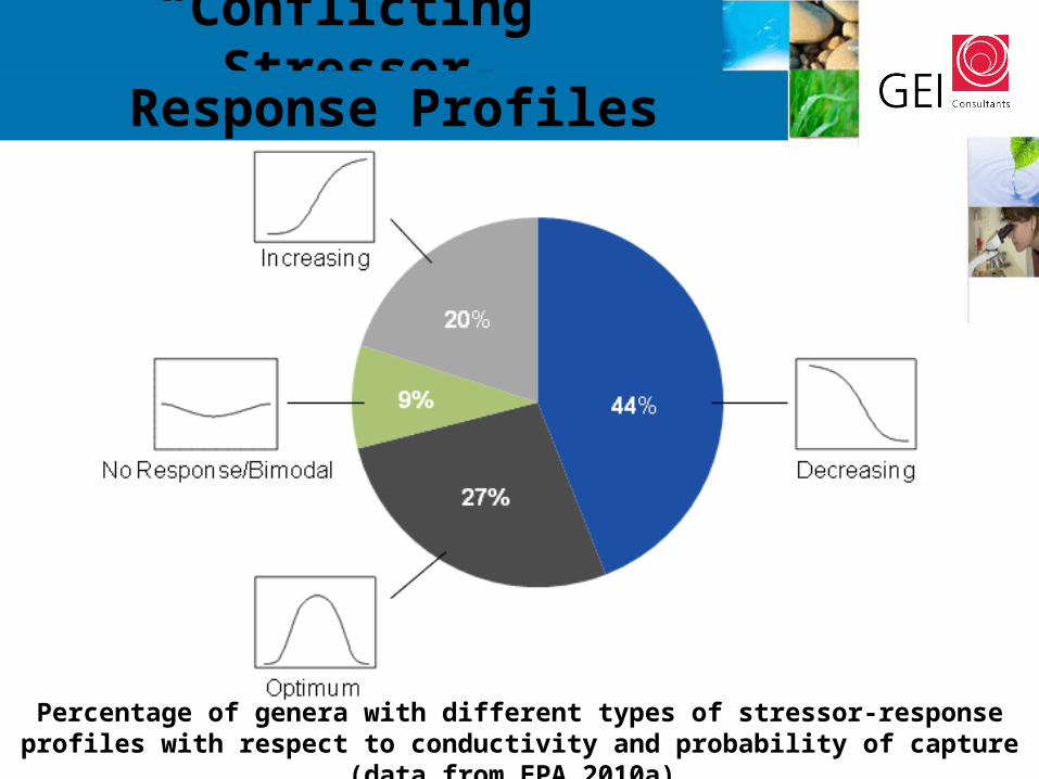
Percentage of genera with different types of stressor-response profiles with respect to conductivity and probability of capture (data from EPA 2010a).

“Conflicting” Stressor-Response Profiles

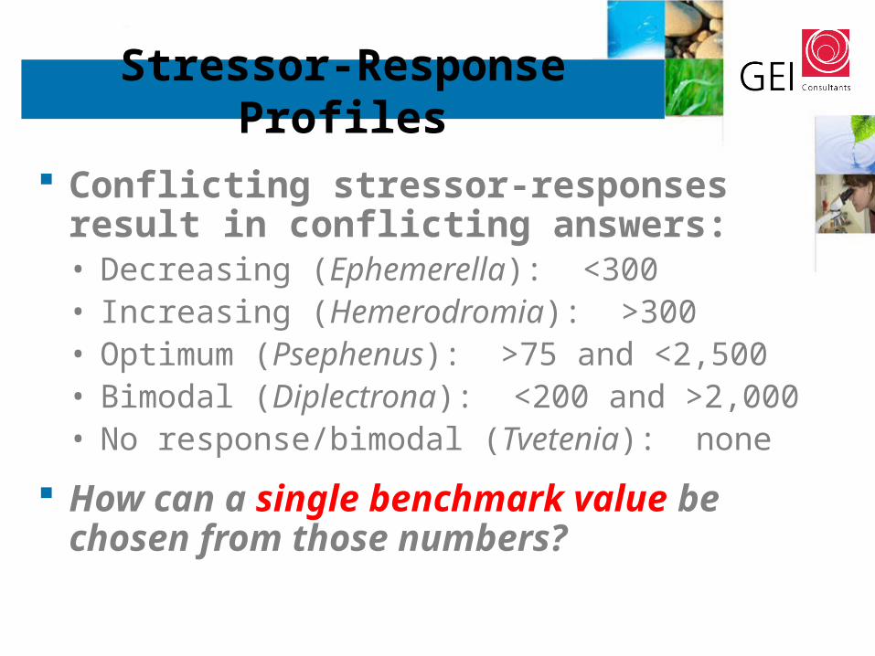
Conflicting stressor-responses result in conflicting answers:• Decreasing (Ephemerella): <300• Increasing (Hemerodromia): >300• Optimum (Psephenus): >75 and <2,500• Bimodal (Diplectrona): <200 and >2,000• No response/bimodal (Tvetenia): none

How can a single benchmark value be chosen from those numbers?

Stressor-Response Profiles

Incomplete analysis of causality• Correlation ≠ causality!• Limited experimental evidence

(few laboratory studies)

Confounding factors dismissed inappropriately• Takes causality of conductivity “as a given”• Important factors dismissed

– Habitat, flow, substrate characteristics, etc., widely known to influence species composition

10

“Today's scientists have substituted mathematics for experiments, … and eventually build a structure which has no relation to reality”

– Nikola Tesla

Primary Technical Concerns

Goal: “establish that salts are a general cause, not that they cause all impairments, nor that there are no other causes of impairment, nor that they cause the impairment at any particular site.” (emphasis added)

Epidemiological approaches used• 6 characteristics of causation

– Co-occurrence, preceding causation, time order, interaction, alteration, sufficiency

– Weight of evidence scoring

• Concluded that salts (measured by conductivity) are common cause of aquatic macroinvertebrates impairment

Our conclusion: This is an incomplete analysis• Weight of evidence scoring for each element relatively subjective‒ Open to valid alternative interpretations • Limited experimental evidence– Few toxicity tests– No experimental verification of extirpation in whole communities

11

EPA Approach:Causality

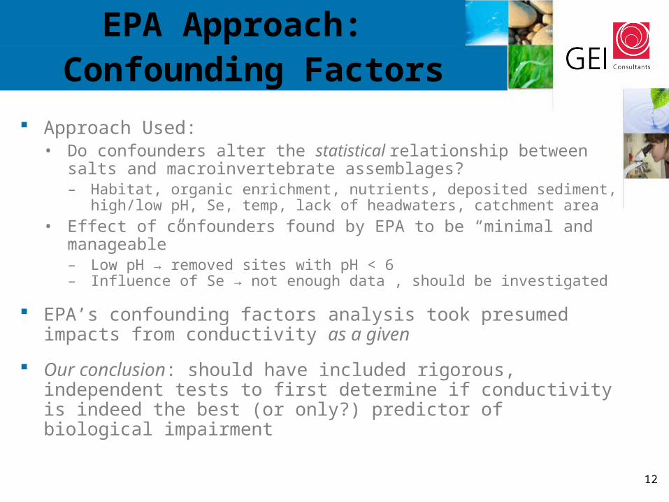
Approach Used:• Do confounders alter the statistical relationship between salts and

macroinvertebrate assemblages?– Habitat, organic enrichment, nutrients, deposited sediment, high/low pH,

Se, temp, lack of headwaters, catchment area

• Effect of confounders found by EPA to be “minimal and manageable”– Low pH → removed sites with pH < 6– Influence of Se → not enough data , should be investigated

EPA’s confounding factors analysis took presumed impacts from conductivity as a given

Our conclusion: should have included rigorous, independent tests to first determine if conductivity is indeed the best (or only?) predictor of biological impairment

12

EPA Approach:Confounding Factors

EPA Approach:

• What about alternative explanations for community structure patterns?

Habitat:1. RBP scores not best measure of macroinvertebrate habitat quality2. RBP scores correlated with conductivity and biological response3. Analysis focused on relationship with Ephemeroptera (mayflies)

Excluded the rest of the benthic macroinvertebrate community

Relationship to other invertebrate taxa: 1. Relationships with Ephemeroptera used to reject other stressors as potential

confounders2. Should include analyses for other invertebrates

Again, excluded the rest of the community -- Protect all invertebrates, not just mayflies!

13

Confounding Factors

Independent analysis that considered additional information• Identify key WQ and physical parameters most strongly

associated with biotic responses• Minimize use of composite variables (e.g., conductivity)

West Virginia Department of Environmental Protection (WVDEP) Watershed Assessment Branch Database (WABbase) – same as used by EPA• Results for 3,286 sampling events

– 3,121 unique Station ID codes

• A variety of site-specific data– Regional landscape– Water quality– Aquatic habitat conditions– Macroinvertebrate community composition

14

Our Approach:ID Additional Confounders

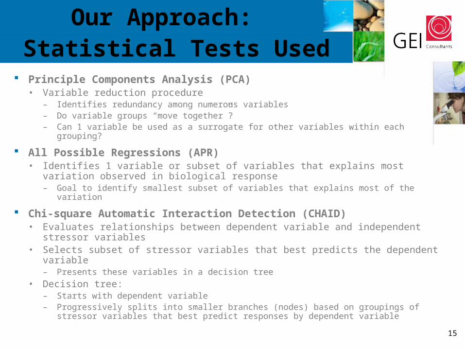
Principle Components Analysis (PCA)• Variable reduction procedure

– Identifies redundancy among numerous variables– Do variable groups “move together”?– Can 1 variable be used as a surrogate for other variables within each grouping?

All Possible Regressions (APR) • Identifies 1 variable or subset of variables that explains most variation observed

in biological response– Goal to identify smallest subset of variables that explains most of the variation

Chi-square Automatic Interaction Detection (CHAID) • Evaluates relationships between dependent variable and independent stressor

variables• Selects subset of stressor variables that best predicts the dependent variable

– Presents these variables in a decision tree

• Decision tree:– Starts with dependent variable– Progressively splits into smaller branches (nodes) based on groupings of stressor

variables that best predict responses by dependent variable 15

Our Approach:Statistical Tests Used

16

Principal ComponentAnalysis All Possible Regressions

Chi-square Automatic Interaction Detection

Genera-based Total TaxaTotal magnesium Undisturbed vegetation SulfatePercent fines Channel alteration Channel alteration

Sulfate Total magnesiumEmbeddednessEpifaunal substrate

Percent EPTPercent fines Undisturbed vegetation Epifaunal substrateTotal magnesium Epifaunal substrate Fecal coliformsTotal suspended solids Fecal coliforms Bank vegetation

Chloride pHTotal manganese

Independent stressors most closely associated with key dependent responses (genera-based total taxa and percent EPT):

Statistical Conclusions

17

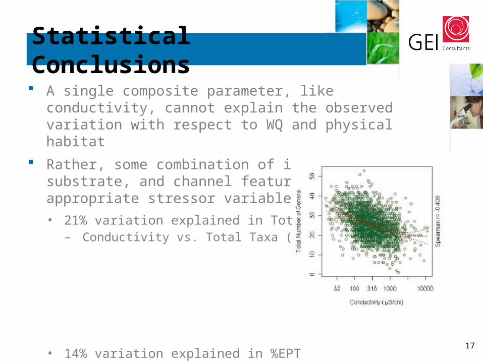
A single composite parameter, like conductivity, cannot explain the observed variation with respect to WQ and physical habitat

Rather, some combination of ionic composition, substrate, and channel features may be the most appropriate stressor variables to consider

• 21% variation explained in Total Taxa– Conductivity vs. Total Taxa (r 2 = 0.18)

• 14% variation explained in %EPT– Conductivity vs. % EPT Abundance (r 2 = 0.08)

Statistical Conclusions

Illinois sulfate criterion

<1% of WABbase samples exceeded the IL sulfate criteria• Majority of exceedances occurred with hardness levels >500 mg/L

26% of these WABbase samples exceed the proposed conductivity benchmark

18

Alternative Approach:Single Ion Criteria

Ion RangesChloride<5 mg/L

Chloride5 to <25 mg/L

Chloride25 to <500 mg/L

Chloride≥500 mg/L

Hardness<100 mg/L

500n = 696

500n = 350

500n = 23

500n = 0

Hardness100 to <500 mg/L

500n = 113

Eqn 1n = 84

1 of 84 exceeded criteria

Eqn 2n = 270

2,000n = 1

Hardness≥500 mg/L

500n = 10

6 of 10 exceeded criteria

2,000n = 26

2,000n = 15

7 of 15 exceeded criteria

2,000n = 3

1 of 3 exceeded criteria

Eqn 1: Sulfate = [-57.478 + 5.79(Hardness) + 54.163(Chloride)] x 0.65

Eqn 2: Sulfate = [1,276.7 + 5.508(Hardness) – 1.457(Chloride)] x 0.65

Conclusions

Relationship between conductivity and changes in macroinvertebrate community structure not strong or reliable enough to derive a benchmark

EPA (2010) did not rigorously test primary hypothesis that conductivity is best predictor of changes in macroinvertebrate community structure• Instead, their analysis takes it as a given that conductivity is the best predictor• Confounding factors prematurely dismissed

Insufficient experimental confirmation of the proposed benchmark• For similar reasons, IL, IN, and IA rejected the use of TDS or conductivity-based

criteria in lieu of criteria for individual ions (sulfate or chloride)

19

Conclusions

It is inappropriate and inadvisable to adopt a conductivity benchmark at this time• Many factors other than WQ are strongly related to

macroinvertebrate community structure

To adopt this benchmark without additional study runs a risk of expending financial resources to reduce conductivity• Little confidence that mitigating conductivity alone

would provide any measureable environmental benefit

20

Acknowledgements

We would like to thank:

The National Mining Association

21

bgensemer@geiconsultants.com22