Shri Vishnu Engineering College for Women :: Bhimavaram

Department of Electronics & Communication Engineering

Digital Communication

UNIT I

PULSE DIGITAL MODULATION

Digital Transmission is the transmittal of digital signals between two or more points in a

communications system. The signals can be binary or any other form of discrete-level digital pulses.

Digital pulses can not be propagated through a wireless transmission system such as earth’s

atmosphere or free space.

Alex H. Reeves developed the first digital transmission system in 1937 at the Paris

Laboratories of AT & T for the purpose of carrying digitally encoded analog signals, such as the

human voice, over metallic wire cables between telephone offices.

Advantages & disadvantages of Digital Transmission

Advantages

--Noise immunity

--Multiplexing(Time domain)

--Regeneration

--Simple to evaluate and measure

Disadvantages

--Requires more bandwidth

--Additional encoding (A/D) and decoding (D/A) circuitry

Pulse Modulation

--Pulse modulation consists essentially of sampling analog information signals and then converting

those samples into discrete pulses and transporting the pulses from a source to a destination over a

physical transmission medium.

--The four predominant methods of pulse modulation:

1) pulse width modulation (PWM)

2) pulse position modulation (PPM)

3) pulse amplitude modulation (PAM)

4) pulse code modulation (PCM).

Pulse Width Modulation

--PWM is sometimes called pulse duration modulation (PDM) or pulse length modulation (PLM), as

the width (active portion of the duty cycle) of a constant amplitude pulse is varied proportional to the

amplitude of the analog signal at the time the signal is sampled.

--The maximum analog signal amplitude produces the widest pulse, and the minimum analog signal

amplitude produces the narrowest pulse. Note, however, that all pulses have the same amplitude.

Pulse Position Modulation

--With PPM, the position of a constant-width pulse within a prescribed time slot is varied according to

the amplitude of the sample of the analog signal.

--The higher the amplitude of the sample, the farther to the right the pulse is positioned within the

prescribed time slot. The highest amplitude sample produces a pulse to the far right, and the lowest

amplitude sample produces a pulse to the far left.

Pulse Amplitude Modulation

--With PAM, the amplitude of a constant width, constant-position pulse is varied according to the

amplitude of the sample of the analog signal.

--The amplitude of a pulse coincides with the amplitude of the analog signal.

--PAM waveforms resemble the original analog signal more than the waveforms for PWM or PPM.

Pulse Code Modulation

--With PCM, the analog signal is sampled and then converted to a serial n-bit binary code for

transmission.

--Each code has the same number of bits and requires the same length of time for transmission.

Pulse Modulation

--PAM is used as an intermediate form of modulation with PSK, QAM, and PCM, although it is

seldom used by itself.

--PWM and PPM are used in special-purpose communications systems mainly for the military but are

seldom used for commercial digital transmission systems.

--PCM is by far the most prevalent form of pulse modulation and will be discussed in more detail.

Pulse Code Modulation

--PCM is the preferred method of communications within the public switched telephone network

because with PCM it is easy to combine digitized voice and digital data into a single, high-speed

digital signal and propagate it over either metallic or optical fiber cables.

--With PCM, the pulses are of fixed length and fixed amplitude.

--PCM is a binary system where a pulse or lack of a pulse within a prescribed time slot represents

either a logic 1 or a logic 0 condition.

--PWM, PPM, and PAM are digital but seldom binary, as a pulse does not represent a single binary

digit (bit).

PCM system Block Diagram

--The band pass filter limits the frequency of the analog input signal to the standard voice-band

frequency range of 300 Hz to 3000 Hz.

--The sample- and- hold circuit periodically samples the analog input signal and converts those

samples to a multilevel PAM signal.

--The analog-to-digital converter (ADC) converts the PAM samples to parallel PCM codes, which are

converted to serial binary data in the parallel-to-serial converter and then outputted onto the

transmission linear serial digital pulses.

--The transmission line repeaters are placed at prescribed distances to regenerate the digital pulses.

--In the receiver, the serial-to-parallel converter converts serial pulses received from the transmission

line to parallel PCM codes.

--The digital-to-analog converter (DAC) converts the parallel PCM codes to multilevel PAM signals.

--The hold circuit is basically a low pass filter that converts the PAM signals back to its original

analog form.

The block diagram of a single-channel, simplex (one-way only) PCM system.

PCM Sampling:

--The function of a sampling circuit in a PCM transmitter is to periodically sample the continually

changing analog input voltage and convert those samples to a series of constant- amplitude pulses that

can more easily be converted to binary PCM code.

--A sample-and-hold circuit is a nonlinear device (mixer) with two inputs: the sampling pulse and the

analog input signal.

--For the ADC to accurately convert a voltage to a binary code, the voltage must be relatively constant

so that the ADC can complete the conversion before the voltage level changes. If not, the ADC would

be continually attempting to follow the changes and may never stabilize on any PCM code.

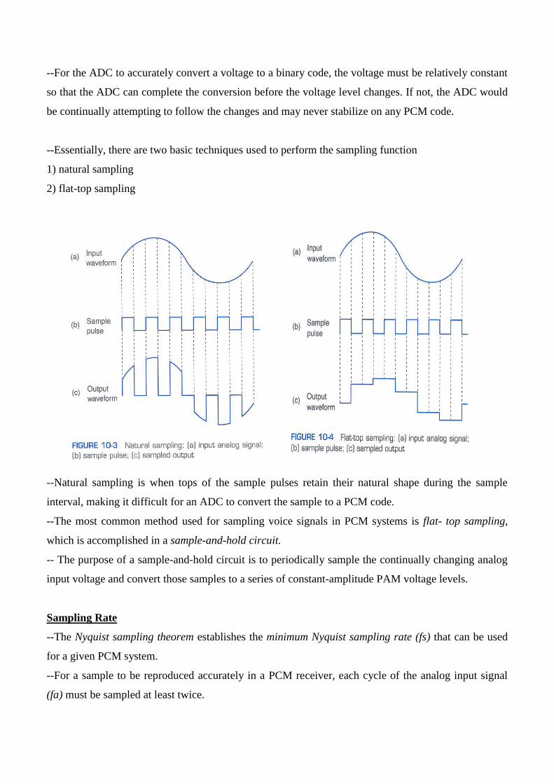
--Essentially, there are two basic techniques used to perform the sampling function

1) natural sampling

2) flat-top sampling

--Natural sampling is when tops of the sample pulses retain their natural shape during the sample

interval, making it difficult for an ADC to convert the sample to a PCM code.

--The most common method used for sampling voice signals in PCM systems is flat- top sampling,

which is accomplished in a sample-and-hold circuit.

-- The purpose of a sample-and-hold circuit is to periodically sample the continually changing analog

input voltage and convert those samples to a series of constant-amplitude PAM voltage levels.

Sampling Rate

--The Nyquist sampling theorem establishes the minimum Nyquist sampling rate (fs) that can be used

for a given PCM system.

--For a sample to be reproduced accurately in a PCM receiver, each cycle of the analog input signal

(fa) must be sampled at least twice.

--Consequently, the minimum sampling rate is equal to twice the highest audio input frequency.

--Mathematically, the minimum Nyquist sampling rate is:

fs ≥ 2fa

--If fs is less than two times fa an impairment called alias or foldover distortion occurs.

Quantization and the Folded Binary Code:

Quantization

--Quantization is the process of converting an infinite number of possibilities to a finite number of

conditions.

--Analog signals contain an infinite number of amplitude possibilities.

--Converting an analog signal to a PCM code with a limited number of combinations requires

quantization.

Folded Binary Code

--With quantization, the total voltage range is subdivided into a smaller number of sub-ranges.

--The PCM code shown in Table 10-2 is a three-bit sign- magnitude code with eight possible

combinations (four positive and four negative).

--The leftmost bit is the sign bit (1 = + and 0 = -), and the two rightmost bits represent magnitude.

-- This type of code is called a folded binary code because the codes on the bottom half of the table

are a mirror image of the codes on the top half, except for the sign bit.

Quantization

--With a folded binary code, each voltage level has one code assigned to it except zero volts, which

has two codes, 100 (+0) and 000 (-0).

--The magnitude difference between adjacent steps is called the quantization interval or quantum.

--For the code shown in Table 10-2, the quantization interval is 1 V.

--If the magnitude of the sample exceeds the highest quantization interval, overload distortion (also

called peak limiting) occurs.

--Assigning PCM codes to absolute magnitudes is called quantizing.

--The magnitude of a quantum is also called the resolution.

--The resolution is equal to the voltage of the minimum step size, which is equal to the voltage of the

least significant bit (Vlsb) of the PCM code.

--The smaller the magnitude of a quantum, the better (smaller) the resolution and the more accurately

the quantized signal will resemble the original analog sample.

--For a sample, the voltage at t3 is approximately +2.6 V. The folded PCM code is

sample voltage = 2.6 = 2.6

resolution 1

--There is no PCM code for +2.6; therefore, the magnitude of the sample is rounded off to the nearest

valid code, which is 111, or +3 V.

--The rounding-off process results in a quantization error of 0.4 V.

--The likelihood of a sample voltage being equal to one of the eight quantization levels is remote.

--Therefore, as shown in the figure, each sample voltage is rounded off (quantized) to the closest

available level and then converted to its corresponding PCM code.

--The rounded off error is called the called the quantization error (Qe).

--To determine the PCM code for a particular sample voltage, simply divide the voltage by the

resolution, convert the quotient to an n-bit binary code, and then add the sign bit.

1) For the PCM coding scheme shown in Figure 10-8, determine the quantized voltage, quantization

error (Qe) and PCM code for the analog sample voltage of + 1.07 V.

A) To determine the quantized level, simply divide the sample voltage by resolution and then round

the answer off to the nearest quantization level:

+1.07V = 1.07 = 1

1V

The quantization error is the difference between the original sample voltage and the quantized level, or

Qe = 1.07 -1 = 0.07

From Table 10-2, the PCM code for + 1 is 101.

Dynamic Range (DR): It determines the number of PCM bits transmitted per sample.

-- Dynamic range is the ratio of the largest possible magnitude to the smallest possible magnitude

(other than zero) that can be decoded by the digital-to-analog converter in the receiver. Mathematically,

=20 log Vmax

Vmin

where DR = dynamic range (unitless)

Vmin = the quantum value

Vmax = the maximum voltage magnitude of the DACs

n = number of bits in a PCM code (excluding the sign bit)

For n > 4

max max

min

2 1resolution

nV VDR

V 20log 2 1n

dBDR

2 1 2n nDR

20log 2 1 20 log2 6n

dBDR n n

Signal-to-Quantization Noise Efficiency

--For linear codes, the magnitude change between any two successive codes is the same.

--Also, the magnitude of their quantization error is also same.

The maximum quantization noise is half the resolution. Therefore, the worst possible signal voltage-

to-quantization noise voltage ratio (SQR) occurs when the input signal is at its minimum amplitude

(101 or 001). Mathematically, the worst-case voltage SQR is

SQR = resolution = Vlsb =2

Qe V lsb /2

For input signal minimum amplitude

SQR = minimum voltage / quantization noise

For input signal maximum amplitude

SQR = maximum voltage / quantization noise

SQR is not constant where R = resistance (ohms)

SQR (dB) = 10 log v2 /R v = rms signal voltage (volts)

(q 2 /12)/R q = quantization interval (volts)

v2

/R = average signal power (watts)

(q 2 /12)/R = average quantization noise power (watts)

Companding

--Companding is the process of compressing and then expanding

--High amplitude analog signals are compressed prior to txn. and then expanded in the receiver

--Higher amplitude analog signals are compressed and Dynamic range is improved

--Early PCM systems used analog companding, where as modern systems use digital companding.

resolution

2eQ

min

min

resolution2

e e

VSQR

Q Q

max

max

e

VSQR

Q

Analog companding

PCM system with analog companding

--In the transmitter, the dynamic range of the analog signal is compressed, and then converted o a

linear PCM code.

--In the receiver, the PCM code is converted to a PAM signal, filtered, and then expanded back to its

original dynamic range.

-- There are two methods of analog companding currently being used that closely approximate a

logarithmic function and are often called log-PCM codes.

The two methods are 1) -law and

2) A-law

-law companding

where Vmax = maximum uncompressed analog input amplitude(volts)

Vin = amplitude of the input signal at a particular instant of time (volts)

= parameter used tio define the amount of compression (unitless)

Vout = compressed output amplitude (volts)

A-law companding

--A-law is superior to -law in terms of small-signal quality

--The compression characteristic is given by

where y = Vout

x = Vin / Vmax

Digital Companding: Block diagram refer in text book.

--With digital companding, the analog signal is first sampled and converted to a linear PCM code, and

then the linear code is digitally compressed.

-- In the receiver, the compressed PCM code is expanded and then decoded back to analog.

-- The most recent digitally compressed PCM systems use a 12- bit linear PCM code and an 8-bit

compressed PCM code.

maxmax

ln 1

ln 1

in

out

VV

VV

1||1

,log1

|)|log(1

1||0,

log1

||

xAA

xAA

xA

xA

y

Digital compression error

--To calculate the percentage error introduced by digital compression

%error=12-bit encoded voltage - 12-bit decoded voltage X 100

12-bit decoded voltage

PCM Line speed

--Line speed is the data rate at which serial PCM bits are clocked out of the PCM encoder onto the

transmission line. Mathematicaly,

Line speed= samples X bits

second sample

Delta Modulation

--Delta modulation uses a single-bit PCM code to achieve digital transmission of analog signals.

--With conventional PCM, each code is a binary representation of both the sign and the magnitude of a

particular sample. Therefore, multiple-bit codes are required to represent the many values that the

sample can be.

--With delta modulation, rather than transmit a coded representation of the sample, only a single bit is

transmitted, which simply indicates whether that sample is larger or smaller than the previous sample.

--The algorithm for a delta modulation system is quite simple.

--If the current sample is smaller than the previous sample, a logic 0 is transmitted.

--If the current sample is larger than the previous sample, a logic 1 is transmitted.

Differential DM

--With Differential Pulse Code Modulation (DPCM), the difference in the amplitude of two successive

samples is transmitted rather than the actual sample. Because the range of sample differences is

typically less than the range of individual samples, fewer bits are required for DPCM than

conventional PCM.

UNIT II

DELTA MODULATION

Delta modulation (DM or Δ-modulation)is an analog-to-digital and digital-to-analog signal

conversion technique used for transmission of voice information where quality is not of primary

importance. DM is the simplest form of differential pulse-code modulation (DPCM) where the

differences between successive samples are encoded into n-bit data streams. In delta modulation, the

transmitted data is reduced to a 1-bit data stream.

Its main features are:

the analog signal is approximated with a series of segments

each segment of the approximated signal is compared to the original analog wave to determine

the increase or decrease in relative amplitude

the decision process for establishing the state of successive bits is determined by this

comparison

only the change of information is sent, that is, only an increase or decrease of the signal

amplitude from the previous sample is sent whereas a no-change condition causes the

modulated signal to remain at the same 0 or 1 state of the previous sample.

To achieve high signal-to-noise ratio, delta modulation must use oversampling techniques, that is, the

analog signal is sampled at a rate several times higher than the Nyquist rate.

Derived forms of delta modulation are continuously variable slope delta modulation, delta-sigma

modulation, and differential modulation. Differential pulse-code modulation is the super set of DM.

Principle

Rather than quantizing the absolute value of the input analog waveform, delta modulation quantizes

the difference between the current and the previous step, as shown in the below block diagram.

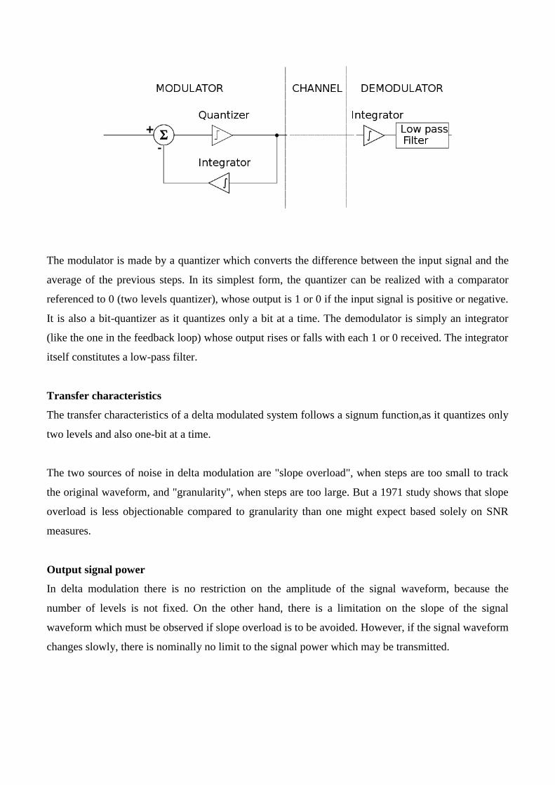
The modulator is made by a quantizer which converts the difference between the input signal and the

average of the previous steps. In its simplest form, the quantizer can be realized with a comparator

referenced to 0 (two levels quantizer), whose output is 1 or 0 if the input signal is positive or negative.

It is also a bit-quantizer as it quantizes only a bit at a time. The demodulator is simply an integrator

(like the one in the feedback loop) whose output rises or falls with each 1 or 0 received. The integrator

itself constitutes a low-pass filter.

Transfer characteristics

The transfer characteristics of a delta modulated system follows a signum function,as it quantizes only

two levels and also one-bit at a time.

The two sources of noise in delta modulation are "slope overload", when steps are too small to track

the original waveform, and "granularity", when steps are too large. But a 1971 study shows that slope

overload is less objectionable compared to granularity than one might expect based solely on SNR

measures.

Output signal power

In delta modulation there is no restriction on the amplitude of the signal waveform, because the

number of levels is not fixed. On the other hand, there is a limitation on the slope of the signal

waveform which must be observed if slope overload is to be avoided. However, if the signal waveform

changes slowly, there is nominally no limit to the signal power which may be transmitted.

Bit-rate

If the communication channel is of limited bandwidth, there is the possibility of interference in either

DM or PCM. Hence, 'DM' and 'PCM' operate at same bit-rate.[dubious – discuss]

Adaptive delta modulation

Adaptive delta modulation (ADM) or continuously variable slope delta modulation (CVSD) is a

modification of DM in which the step size is not fixed. Rather, when several consecutive bits have the

same direction value, the encoder and decoder assume that slope overload is occurring, and the step

size becomes progressively larger. Otherwise, the step size becomes gradually smaller over time.

ADM reduces slope error, at the expense of increasing quantizing error. This error can be reduced by

using a low pass filter.

ADM provides robust performance in the presence of bit errors meaning error detection and correction

are not typically used in an ADM radio design, this allows for a reduction in host processor workload

(allowing a low-cost processor to be used).

Applications

A contemporary application of Delta Modulation includes, but is not limited to, recreating legacy

synthesizer waveforms. With the increasing availability of FPGAs and game-related ASICs, sample

rates are easily controlled so as to avoid slope overload and granularity issues. For example, the

C64DTV used a 32MHz sample rate, providing ample dynamic range to recreate the SID output to

acceptable levels

SBS Application 24Kbps Delta Modulation

Delta Modulation was used by Satellite Business Systems or SBS for its voice ports to provide long

distance phone service to large domestic corporations with a significant inter-corporation

communications need (such as IBM). This system was in service throughout the 1980s. The voice

ports used digitally implemented 24kbit/s Delta Modulation with Voice Activity Compression or VAC

and Echo Suppressors to control the half second echo path through the satellite. They performed

formal listening tests to verify the 24kbit/s Delta Modulator achieved full voice quality with no

discernable degradation as compared to a high quality phone line or the standard 64kbit/s µ-law

Companded PCM. This provided an eight to three improvement in satellite channel capacity. IBM

developed the Satellite Communications Controller and the voice port functions.

The original proposal in 1974 used a state-of-the-art 24kbit/s Delta Modulator with a single integrator

and a Shindler Compander modified for gain error recovery. This proved to have less than full phone

line speech quality. In 1977one engineer with two assistants in the IBM Research Triangle Park, NC

laboratory was assigned to improve the quality.

The final implementation replaced the integrator with a Predictor implemented with a two pole

complex pair low pass filter designed to approximate the long term average speech spectrum. The

theory was that ideally the integrator should be a predictor designed to match the signal spectrum. A

nearly perfect Shindler Compander replaced the modified version. It was found the modified

compander resulted in a less than perfect step size at most signal levels and the fast gain error recovery

increased the noise as determined by actual listening tests as compared to simple signal to noise

measurements. The final compander achieved a very mild gain error recovery due to the natural

truncation rounding error caused by twelve bit arithmetic.

The complete function of Delta Modulation, VAC and Echo Control for six ports was implemented in

a single digital integrated circuit chip with twelve bit arithmetic. A single DAC was shared by all six

ports providing voltage compare functions for the modulators and feeding sample and hold circuits for

the demodulator outputs. A single card held the chip, DAC and all the analog circuits for the phone

line interface including transformers.

UNIT III

DELTA MODULATION

Digital modulation methods

In digital modulation, an analog carrier signal is modulated by a discrete signal. Digital modulation

methods can be considered as digital-to-analog conversion, and the corresponding demodulation or

detection as analog-to-digital conversion. The changes in the carrier signal are chosen from a finite

number of M alternative symbols (the modulation alphabet).

Schematic of 4 baud (8 bit/s) data link containing arbitrarily chosen values.

A simple example: A telephone line is designed for transferring audible sounds, for example tones,

and not digital bits (zeros and ones). Computers may however communicate over a telephone line by

means of modems, which are representing the digital bits by tones, called symbols. If there are four

alternative symbols (corresponding to a musical instrument that can generate four different tones, one

at a time), the first symbol may represent the bit sequence 00, the second 01, the third 10 and the

fourth 11. If the modem plays a melody consisting of 1000 tones per second, the symbol rate is 1000

symbols/second, or baud. Since each tone (i.e., symbol) represents a message consisting of two digital

bits in this example, the bit rate is twice the symbol rate, i.e. 2000 bits per second. This is similar to

the technique used by dialup modems as opposed to DSL modems.

According to one definition of digital signal, the modulated signal is a digital signal, and according to

another definition, the modulation is a form of digital-to-analog conversion. Most textbooks would

consider digital modulation schemes as a form of digital transmission, synonymous to data

transmission; very few would consider it as analog transmission.

Fundamental digital modulation methods

The most fundamental digital modulation techniques are based on keying:

PSK (phase-shift keying): a finite number of phases are used.

FSK (frequency-shift keying): a finite number of frequencies are used.

ASK (amplitude-shift keying): a finite number of amplitudes are used.

QAM (quadrature amplitude modulation): a finite number of at least two phases and at least

two amplitudes are used.

For determining error-rates mathematically, some definitions will be needed:

= Energy-per-bit

= Energy-per-symbol = with n bits per symbol

= Bit duration

= Symbol duration

= Noise power spectral density (W/Hz)

= Probability of bit-error

= Probability of symbol-error

will give the probability that a single sample taken from a random process with zero-mean and

unit-variance Gaussian probability density function will be greater or equal to . It is a scaled form of

the complementary Gaussian error function:

.

The error-rates quoted here are those in additive white Gaussian noise (AWGN). These error rates are

lower than those computed in fading channels, hence, are a good theoretical benchmark to compare

with.

In QAM, an inphase signal (or I, with one example being a cosine waveform) and a quadrature phase

signal (or Q, with an example being a sine wave) are amplitude modulated with a finite number of

amplitudes, and then summed. It can be seen as a two-channel system, each channel using ASK. The

resulting signal is equivalent to a combination of PSK and ASK.

In all of the above methods, each of these phases, frequencies or amplitudes are assigned a unique

pattern of binary bits. Usually, each phase, frequency or amplitude encodes an equal number of bits.

This number of bits comprises the symbol that is represented by the particular phase, frequency or

amplitude.

If the alphabet consists of M = 2^N alternative symbols, each symbol represents a message consisting

of N bits. If the symbol rate (also known as the baud rate) is f_{S} symbols/second (or baud), the data

rate is N f_{S} bit/second.

In the case of PSK, ASK or QAM, where the carrier frequency of the modulated signal is constant, the

modulation alphabet is often conveniently represented on a constellation diagram, showing the

amplitude of the I signal at the x-axis, and the amplitude of the Q signal at the y-axis, for each symbol.

Phase-shift keying

Phase-shift keying (PSK) is a digital modulation scheme that conveys data by changing, or modulating,

the phase of a reference signal (the carrier wave). Any digital modulation scheme uses a finite number

of distinct signals to represent digital data. PSK uses a finite number of phases, each assigned a unique

pattern of binary digits. Usually, each phase encodes an equal number of bits. Each pattern of bits

forms the symbol that is represented by the particular phase. The demodulator, which is designed

specifically for the symbol-set used by the modulator, determines the phase of the received signal and

maps it back to the symbol it represents, thus recovering the original data. This requires the receiver to

be able to compare the phase of the received signal to a reference signal — such a system is termed

coherent (and referred to as CPSK).

Alternatively, instead of operating with respect to a constant reference wave, the broadcast can operate

with respect to itself. Changes in phase of a single broadcast waveform can be considered the

significant items. In this system, the demodulator determines the changes in the phase of the received

signal rather than the phase (relative to a reference wave) itself. Since this scheme depends on the

difference between successive phases, it is termed differential phase-shift keying (DPSK). DPSK can

be significantly simpler to implement than ordinary PSK since there is no need for the demodulator to

have a copy of the reference signal to determine the exact phase of the received signal (it is a non-

coherent scheme). In exchange, it produces more erroneous demodulation.

Binary phase-shift keying (BPSK)

Constellation diagram example for BPSK

BPSK (also sometimes called PRK, phase reversal keying, or 2PSK) is the simplest form of phase

shift keying (PSK). It uses two phases which are separated by 180° and so can also be termed 2-PSK.

It does not particularly matter exactly where the constellation points are positioned, and in this figure

they are shown on the real axis, at 0° and 180°. This modulation is the most robust of all the PSKs

since it takes the highest level of noise or distortion to make the demodulator reach an incorrect

decision. It is, however, only able to modulate at 1 bit/symbol (as seen in the figure) and so is

unsuitable for high data-rate applications.

In the presence of an arbitrary phase-shift introduced by the communications channel, the demodulator

is unable to tell which constellation point is which. As a result, the data is often differentially encoded

prior to modulation. BPSK is functionally equivalent to 2-QAM modulation.

The general form for BPSK follows the equation:

This yields two phases, 0 and π. In the specific form, binary data is often conveyed with the following

signals:

…for binary "0"

…for binary "1"

where fc is the frequency of the carrier-wave.

Hence, the signal-space can be represented by the single basis function

where 1 is represented by and 0 is represented by . This assignment is, of

course, arbitrary. This use of this basis function is shown at the end of the next section in a signal

timing diagram. The topmost signal is a BPSK-modulated cosine wave that the BPSK modulator

would produce. The bit-stream that causes this output is shown above the signal (the other parts of this

figure are relevant only to QPSK).

Bit error rate

The bit error rate (BER) of BPSK in AWGN can be calculated as:

or

Since there is only one bit per symbol, this is also the symbol error rate.

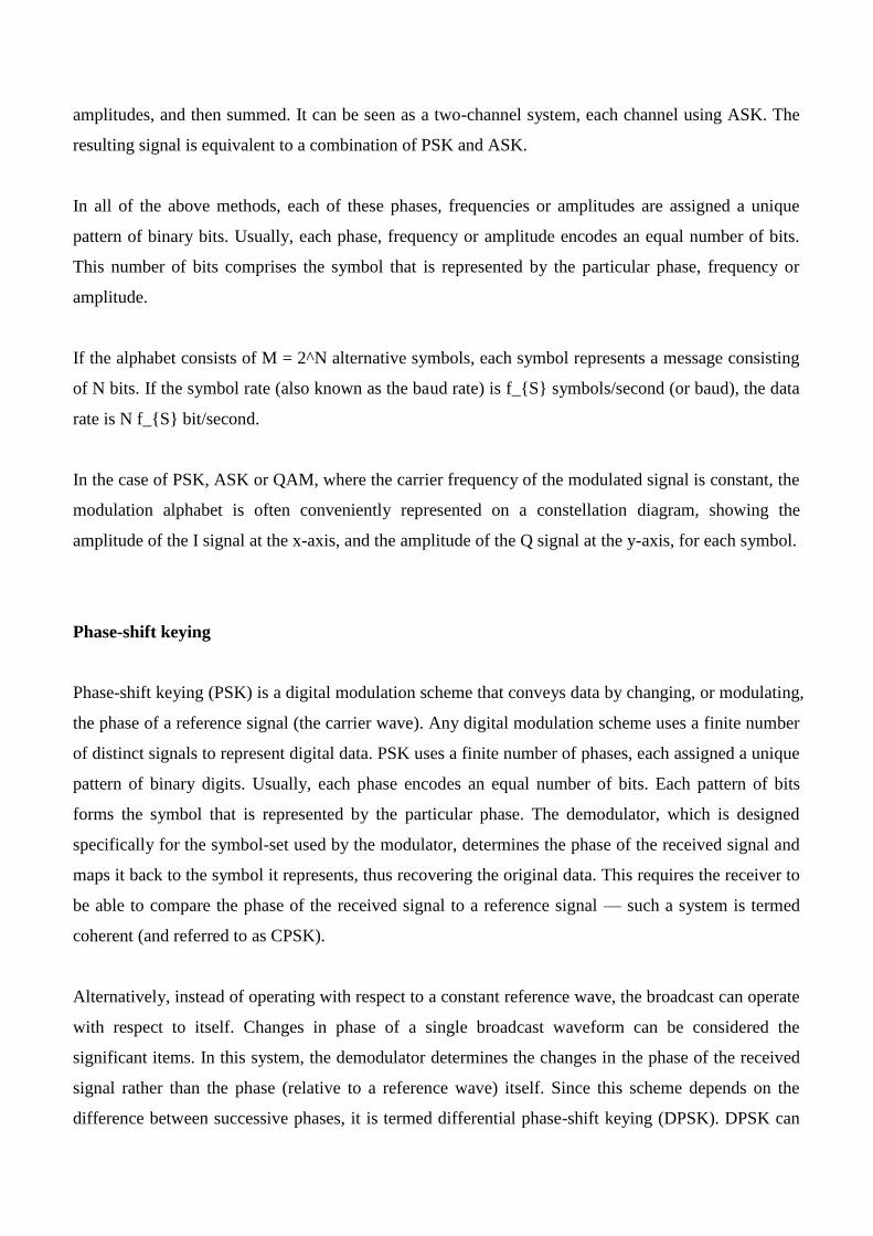
Quadrature phase-shift keying (QPSK)

Constellation diagram for QPSK with Gray coding

Sometimes this is known as quaternary PSK, quadriphase PSK, 4-PSK, or 4-QAM. (Although the root

concepts of QPSK and 4-QAM are different, the resulting modulated radio waves are exactly the

same.) QPSK uses four points on the constellation diagram, equispaced around a circle. With four

phases, QPSK can encode two bits per symbol, shown in the diagram with gray coding to minimize

the bit error rate (BER) — sometimes misperceived as twice the BER of BPSK.

The mathematical analysis shows that QPSK can be used either to double the data rate compared with

a BPSK system while maintaining the same bandwidth of the signal, or to maintain the data-rate of

BPSK but halving the bandwidth needed. In this latter case, the BER of QPSK is exactly the same as

the BER of BPSK - and deciding differently is a common confusion when considering or describing

QPSK.

Given that radio communication channels are allocated by agencies such as the Federal

Communication Commission giving a prescribed (maximum) bandwidth, the advantage of QPSK over

BPSK becomes evident: QPSK transmits twice the data rate in a given bandwidth compared to BPSK -

at the same BER. The engineering penalty that is paid is that QPSK transmitters and receivers are

more complicated than the ones for BPSK. However, with modern electronics technology, the penalty

in cost is very moderate.

As with BPSK, there are phase ambiguity problems at the receiving end, and differentially encoded

QPSK is often used in practice.

The implementation of QPSK is more general than that of BPSK and also indicates the

implementation of higher-order PSK. Writing the symbols in the constellation diagram in terms of the

sine and cosine waves used to transmit them:

This yields the four phases π/4, 3π/4, 5π/4 and 7π/4 as needed.

This results in a two-dimensional signal space with unit basis functions

The first basis function is used as the in-phase component of the signal and the second as the

quadrature component of the signal.

Hence, the signal constellation consists of the signal-space 4 points

The factors of 1/2 indicate that the total power is split equally between the two carriers.

Comparing these basis functions with that for BPSK shows clearly how QPSK can be viewed as two

independent BPSK signals. Note that the signal-space points for BPSK do not need to split the symbol

(bit) energy over the two carriers in the scheme shown in the BPSK constellation diagram.

Bit error rate

Although QPSK can be viewed as a quaternary modulation, it is easier to see it as two independently

modulated quadrature carriers. With this interpretation, the even (or odd) bits are used to modulate the

in-phase component of the carrier, while the odd (or even) bits are used to modulate the quadrature-

phase component of the carrier. BPSK is used on both carriers and they can be independently

demodulated.

As a result, the probability of bit-error for QPSK is the same as for BPSK:

However, in order to achieve the same bit-error probability as BPSK, QPSK uses twice the power

(since two bits are transmitted simultaneously).

The symbol error rate is given by:

If the signal-to-noise ratio is high (as is necessary for practical QPSK systems) the probability of

symbol error may be approximated:

Frequency-shift keying

Frequency-shift keying (FSK) is a frequency modulation scheme in which digital information is

transmitted through discrete frequency changes of a carrier wave.[1] The simplest FSK is binary FSK

(BFSK). BFSK uses a pair of discrete frequencies to transmit binary (0s and 1s) information.[2] With

this scheme, the "1" is called the mark frequency and the "0" is called the space frequency. The time

domain of an FSK modulated carrier is illustrated in the figures to the right.

An example of binary FSK

The demodulation of a binary FSK signal can be done using the Goertzel algorithm very efficiently,

even on low-power microcontrollers.

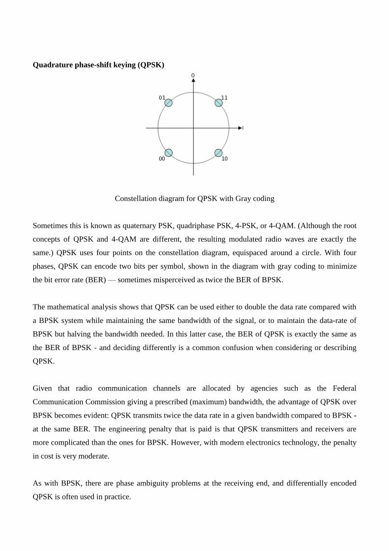
UNIT # V: INFORMATION THEORY

Information theory is a branch of science that deals with the analysis of a

communications system

We will study digital communications – using a file (or network protocol) as the

channel

Claude Shannon Published a landmark paper in 1948 that was the beginning of the

branch of information theory

We are interested in communicating information from a source to a destination

In our case, the messages will be a sequence of binary digits

Does anyone know the term for a binary digit?

One detail that makes communicating difficult is noise

noise introduces uncertainty

Suppose I wish to transmit one bit of information what are all of the possibilities?

tx 0, rx 0 - good

tx 0, rx 1 - error

tx 1, rx 0 - error

tx 1, rx 1 - good

Two of the cases above have errors – this is where probability fits into the picture

In the case of steganography, the ―noise‖ may be due to attacks on the hiding

algorithm

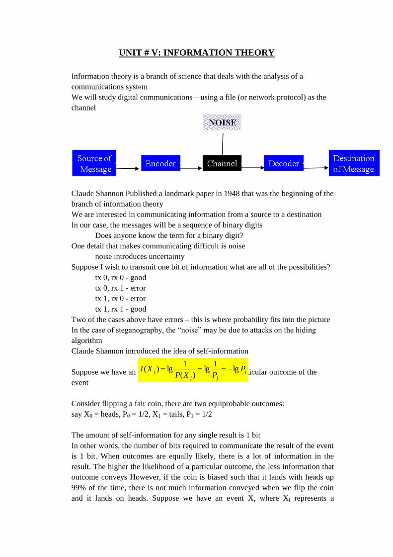
Claude Shannon introduced the idea of self-information

Suppose we have an event X, where Xi represents a particular outcome of the

event

Consider flipping a fair coin, there are two equiprobable outcomes:

say X0 = heads, P0 = 1/2, X1 = tails, P1 = 1/2

The amount of self-information for any single result is 1 bit

In other words, the number of bits required to communicate the result of the event

is 1 bit. When outcomes are equally likely, there is a lot of information in the

result. The higher the likelihood of a particular outcome, the less information that

outcome conveys However, if the coin is biased such that it lands with heads up

99% of the time, there is not much information conveyed when we flip the coin

and it lands on heads. Suppose we have an event X, where Xi represents a

j

jj

j PPXP

XI lg1

lg)(

1lg)(

particular outcome of the event. Consider flipping a coin, however, let’s say there

are 3 possible outcomes: heads (P = 0.49), tails (P=0.49), lands on its side (P =

0.02) – (likely MUCH higher than in reality)

Note: the total probability MUST ALWAYS add up to one

The amount of self-information for either a head or a tail is 1.02 bits

For landing on its side: 5.6 bits

Entropy is the measurement of the average uncertainty of information

We will skip the proofs and background that leads us to the formula for

entropy, but it was derived from required properties

Also, keep in mind that this is a simplified explanation

H – entropy

P – probability

X – random variable with a discrete set of possible outcomes

(X0, X1, X2, … Xn-1) where n is the total number of possibilities

Entropy is greatest when the probabilities of the outcomes are equal

Let’s consider our fair coin experiment again

The entropy H = ½ lg 2 + ½ lg 2 = 1

Since each outcome has self-information of 1, the average of 2 outcomes is

(1+1)/2 = 1

Consider a biased coin, P(H) = 0.98, P(T) = 0.02

H = 0.98 * lg 1/0.98 + 0.02 * lg 1/0.02 =

= 0.98 * 0.029 + 0.02 * 5.643 = 0.0285 + 0.1129 = 0.1414

In general, we must estimate the entropy

The estimate depends on our assumptions about about the structure (read pattern)

of the source of information

Consider the following sequence:

1 2 3 2 3 4 5 4 5 6 7 8 9 8 9 10

Obtaining the probability from the sequence

16 digits, 1, 6, 7, 10 all appear once, the rest appear twice

The entropy H = 3.25 bits

Since there are 16 symbols, we theoretically would need 16 * 3.25 bits to transmit

the information

Consider the following sequence:

1 2 1 2 4 4 1 2 4 4 4 4 4 4 1 2 4 4 4 4 4 4

Obtaining the probability from the sequence

1, 2 four times (4/22), (4/22)

4 fourteen times (14/22)

The entropy H = 0.447 + 0.447 + 0.415 = 1.309 bits

Since there are 22 symbols, we theoretically would need 22 * 1.309 = 28.798 (29)

bits to transmit the information

j

jj

j PPXP

XI lg1

lg)(

1lg)(

1

0

1

0

1lglg)(

n

j j

j

n

j

jjP

PPPXHEntropy

However, check the symbols 12, 44

12 appears 4/11 and 44 appears 7/11

H = 0.530 + 0.415 = 0.945 bits

11 * 0.945 = 10.395 (11) bits to tx the info (38 % less!)

We might possibly be able to find patterns with less entropy

Information

What does a word ―information‖ mean?

There is no some exact definition, however:

Information carries new specific knowledge, which is definitely new for its

recipient;

Information is always carried by some specific carrier in different forms (letters,

digits, different specific symbols, sequences of digits, letters, and symbols , etc.);

Information is meaningful only if the recipient is able to interpret it.

According to the Oxford English Dictionary, the earliest historical meaning of the

word information in English was the act of informing, or giving form or shape to

the mind.

The English word was apparently derived by adding the common "noun of action"

ending "-ation‖

The information materialized is a message.

Information is always about something (size of a parameter, occurrence of an

event, etc).

Viewed in this manner, information does not have to be accurate; it may be a truth

or a lie.

Even a disruptive noise used to inhibit the flow of communication and create

misunderstanding would in this view be a form of information.

However, generally speaking, if the amount of information in the received

message increases, the message is more accurate.

Information Theory

How we can measure the amount of information?

How we can ensure the correctness of information?

What to do if information gets corrupted by errors?

How much memory does it require to store information?

Basic answers to these questions that formed a solid background of the modern

information theory were given by the great American mathematician, electrical

engineer, and computer scientist Claude E. Shannon in his paper ―A

Mathematical Theory of Communication‖ published in ―The Bell System

Technical Journal‖ in October, 1948.

Noisy Channels

A noiseless binary channel 0 0

transmits bits without error: 1 1

What to do if we have a noisy channel and you want to send information across

reliably?

Information Capacity Theorem (Shannon Limit)

The information capacity (or channel capacity) C of a continuous channel with

bandwidth BHertz can be perturbed by additive Gaussian white noise of power

spectral density N0/2,

C=B log2(1+P/N0B) bits/sec

provided bandwidth B satisfies where P is the average transmitted power

P = Eb Rb ( for an ideal system, Rb= C). Eb is the transmitted energy per bit,

Rb is transmission rate.

Shannon Limit

UNIT # VI: SOURCE CODING

A code is defined as an n-tuple of q elements. Where q is any alphabet.

Ex. 1001 n=4, q={1,0}

Ex. 2389047298738904 n=16, q={0,1,2,3,4,5,6,7,8,9}

Ex. (a,b,c,d,e) n=5, q={a,b,c,d,e,…,y,z}

The most common code is when q={1,0}. This is known as a binary code.

The purpose

A message can become distorted through a wide range of unpredictable errors.

• Humans

• Equipment failure

• Lighting interference

• Scratches in a magnetic tape

Why error-correcting code?

To add redundancy to a message so the original message can be recovered if it has

been garbled.

e.g. message = 10

code = 1010101010

Send a message

Source Coding

lossy; may consider semantics of the data

depends on characteristics of the data

e.g. DCT, DPCM, ADPCM, color model transform

A code is

distinct if each code word can be distinguished from every other (mapping is

one-to-one)

uniquely decodable if every code word is identifiable when immersed in a

sequence of code words

e.g., with previous table, message 11 could be defined as either ddddd or bbbbbb

Measure of Information

Consider symbols si and the probability of occurrence of each symbol p(si)

In case of fixed-length coding , smallest number of bits per symbol needed is

L ≥ log2(N) bits per symbol

Example: Message with 5 symbols need 3 bits (L ≥ log25)

Variable-Length Coding- Entropy

What is the minimum number of bits per symbol?

Answer: Shannon’s result – theoretical minimum average number of bits per

code work is known as Entropy (H)

Example

Alphabet = {A, B}

p(A) = 0.4; p(B) = 0.6

Compute Entropy (H)

-0.4*log2 0.4 + -0.6*log2 0.6 = .97 bits

Maximum uncertainty (gives largest H)

occurs when all probabilities are equal

Redundancy

Difference between avg. codeword length (L) and avg. information content

(H)

If H is constant, then can just use L

Relative to the optimal value

Shannon-Fano Algorithm

• Arrange the character set in order of decreasing probability

• While a probability class contains more than one symbol:

– Divide the probability class in two

• so that the probabilities in the two halves are as nearly as

possible equal

– Assign a '1' to the first probability class, and a '0' to the second

n

i

ii spsp1

)(log)( 2

Character

X6

X3

X4

X5

X1

X7

X2

Probability

0.25

0.2

0.15

0.15

0.1

0.1

0.05

1

0

1

0

1

0

1

0

1

01

0

Code

11

10

011

010

001

0001

0000

Huffman Encoding

Statistical encoding

To determine Huffman code, it is useful to construct a binary tree

Leaves are characters to be encoded

Nodes carry occurrence probabilities of the characters belonging to the subtree

Example: How does a Huffman code look like for symbols with statistical

symbol occurrence probabilities:

P(A) = 8/20, P(B) = 3/20, P(C ) = 7/20, P(D) = 2/20?

Step 1 : Sort all Symbols according to their probabilities (left to right) from Smallest

to largest these are the leaves of the Huffman tree

Step 2: Build a binary tree from left toRight

Policy: always connect two smaller nodes together (e.g., P(CE) and P(DA) had both

Probabilities that were smaller than P(B), Hence those two did connect first

Step 3: label left branches of the tree With 0 and right branches of the tree With 1

Step 4: Create Huffman Code

Symbol A = 011

Symbol B = 1

Symbol C = 000

Symbol D = 010

Symbol E = 001

Compression algorithms are of great importance when processing and transmitting

Audio, Images and Video.

UNIT#VII: CHANNEL CODING

Channel Coding in Digital Communication Systems

Encoding

Hamming codes

Hamming [7,4] Code

The seven is the number of digits that make the code.

E.g. 0100101

The four is the number of information digits in the code.

E.g. 0100101

Encoded with a generator matrix. All codes can be formed from row operations on

matrix. The code generator matrix for this presentation is the following:

1000011 0100101

0010110 0001111

1100110 1010101 Possible codes

1001100 0110011

0101010 0011001

1101001 1001010

1111111 0111100

0011001 0000000

kknkk PIG

:

1111000

0110100

1010010

1100001

12827

The distance between two codes u and v is the number of positions which differ

e.g. u=(1,0,0,0,0,1,1)

v=(0,1,0,0,1,0,1)

dist(u,v) = 4

Another definition of distance is wt(u – v) = dist(u,v).

For any u, v, and w in a space V, the following three conditions hold:

Parity-Check Matrix

• The parity check matrix is found by solving the generator matrix for

• For each generator matrix G, there exists an (n – k) x n matrix H, such that the

rows of G are orthogonal to the rows of G; i.e.,

• where HT is the transpose of H, and 0 is an k x (n – k) all zeros matrix .

• The matrix H is called the parity-check matrix, that can be used to decode the

received code words.

Channel Decoding

Syndrome Decoding

Consider a transmitted code cm and y is the received sequence, y can be expressed as,

where e denotes binary error vector.

The decoder calculate product

1111000

0110100

1010010

1100001

G

0),( uudist ),(),( uvdistvudist

),(),(),( wvdistvudistwudist

0TGH

0TGH

3343

33

:

:

1001011

0101101

0011110

xx

T

IP

IP

H

ecy m

t

tt

m

t

m

t

eH

eHHc

Hec

yHs

tyH

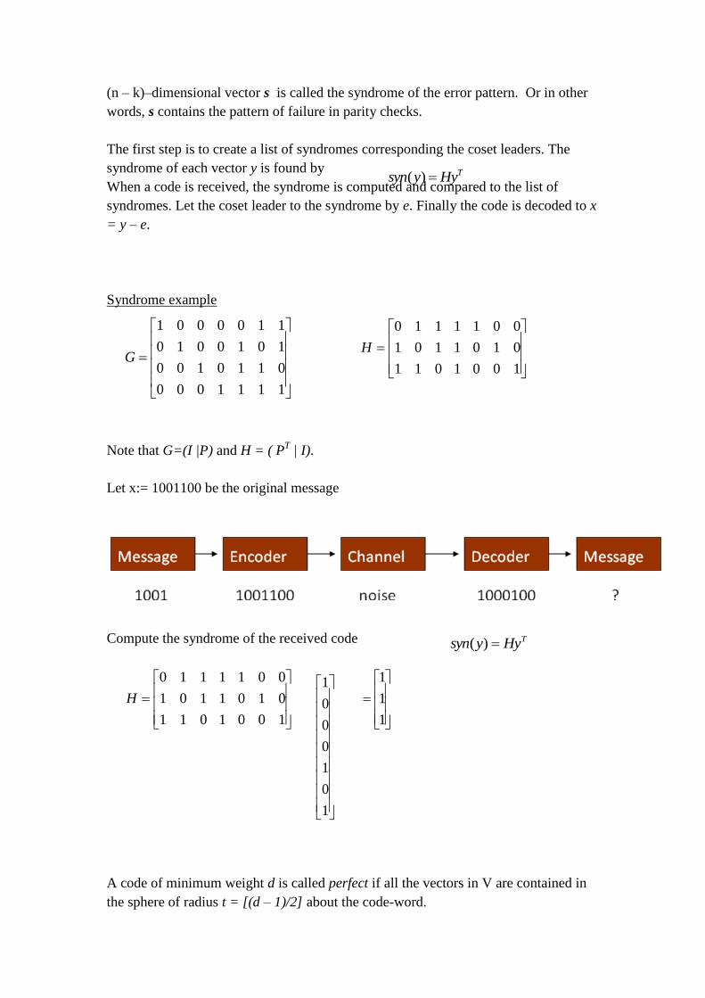
(n – k)–dimensional vector s is called the syndrome of the error pattern. Or in other

words, s contains the pattern of failure in parity checks.

The first step is to create a list of syndromes corresponding the coset leaders. The

syndrome of each vector y is found by

When a code is received, the syndrome is computed and compared to the list of

syndromes. Let the coset leader to the syndrome by e. Finally the code is decoded to x

= y – e.

Syndrome example

Note that G=(I |P) and H = ( PT | I).

Let x:= 1001100 be the original message

Compute the syndrome of the received code

A code of minimum weight d is called perfect if all the vectors in V are contained in

the sphere of radius t = [(d – 1)/2] about the code-word.

THyysyn )(

1111000

0110100

1010010

1100001

G

1001011

0101101

0011110

H

THyysyn )(

1001011

0101101

0011110

H

1

0

1

0

0

0

1

1

1

1

The Hamming [7,4] code has eight vectors of sphere of radius one about each code-

word, times sixteen unique codes. Therefore, the Hamming [7,4] code with minimum

weight 3 is perfect since all the vectors (128) are contained in the sphere of radius 1.

Block Codes

Information is divided into blocks of length k

r parity bits or check bits are added to each block

(total length n = k + r),.

Code rate R = k/n

Decoder looks for codeword closest to received

vector (code vector + error vector)

Tradeoffs between

Efficiency

Reliability

Encoding/Decoding complexity

Block Codes: Linear Block Codes

Linear Block Code

The block length c(x) or C of the Linear Block Code is

c(x) = m(x) g(x) or C= m G

where m(x) or m is the information codeword block length,

g(x)is the generator polynomial, G is the generator matrix.

G = [P | I],

where pi= Remainder of [xn-k+i-1

/g(x)] for i=1, 2, .., k, and I is unit matrix.

The parity check matrix

H = [PT | I], where P

T is the transpose of the matrix P.

Message vector m Generator matrix G Code

Vector C

Code Vector C Parity check matrix HT

Null

Vector 0

Operations of the generator matrix and the parity check matrix

The parity check matrix H is used to detect errors in the received code by using the

fact that c * HT = 0 ( null vector)

Let x=c e be the received message where c is the correct code and e is the error

Compute S=x* HT =( c e)* H

T=c* H

T e* H

T=e* H

T

If S is 0 then message is correct else there are errors in it, from common known error

patterns the correct message can be decoded.

Block Codes: Example

Example : Find linear block code encoder G if code generator polynomial

g(x)=1+x+x3 for a (7, 4) code.

We have n = Total number of bits = 7, k = Number of information bits = 4,

r = Number of parity bits = n - k = 3.

G=[P/I]=

where pi= Remainder of [xn-k+i-1

/g(x)] for i=1, 2, .., k, and I is unit matrix

Cyclic Codes

It is a block code which uses a shift register to perform encoding and decoding

The code word with n bits is expressed as

c(x)=c1xn-1

+c2xn-2

……+ cn

where each ci is either a 1 or 0.

c(x) = m(x) xn-k

+ cp(x)

where cp(x) = remainder from dividing m(x) xn-k

by generator g(x)

if the received signal is c(x) + e(x) where e(x) is the error.

To check if received signal is error free, the remainder from dividing

c(x) + e(x) by g(x) is obtained(syndrome).

If this is 0 then the received signal is considered error free else error pattern is

detected from known error syndromes.

Cyclic Redundancy Check (CRC)

Using parity, some errors are masked - careful choice of bit combinations can lead to

better detection.

Binary (n, k) CRC codes can detect the following error patterns

1. All error bursts of length n-k or less.

2. All combinations of minimum Hamming distance d min - 1 or fewer errors.

.

100

....

0102

0011

pk

p

p

G

3. All error patters with an odd number of errors if the generator polynomial g(x) has

an even number of nonzero coefficients.

Common CRC Codes

Code Generator polynomial g(x) Parity check bits

CRC-12 1+x+x2+x3+x

11+x

12 12

CRC-16 1+x2+x

15+x

16 16

CRC-CCITT 1+x5+x

15+x

16 16