siam math. anal. vol. no. - ucla department of …bertozzi/papers/sima88.pdf · · 2011-03-07siam...

SIAM J. MATH. ANAL.Vol. 19, No. 6, November 1988

1988 Society for Industrial and Applied Mathematics002

HETEROCLINIC ORBITS AND CHAOTIC DYNAMICS IN PLANARFLUID FLOWS*

ANDREA LOUISE BERTOZZI’

Abstract. An extension of the planar Smale-Birkhoff homoclinic theorem to the case of a heteroclinicsaddle connection containing a finite number of fixed points is presented. This extension is used to findchaotic dynamics present in certain time-periodic perturbations of planar fluid models. Specifically, theKelvin-Stuart cat’s eye flow is studied, a model for a vortex pattern found in shear layers. A flow on thetwo-torus with Hamiltonian Ho (27r)- sin (2rx) cos (27rx2) is studied, as well as the evolution equationsfor an elliptical vortex in a three-dimensional strain flow.

Key words, homoclinic orbits, Melnikov’s method, Kelvin-Stuart cat’s eyes, elliptical vortices

AMS(MOS) subject classifications. 34C35, 54H20, 58F08, 58F13, 70K99, 76C05

1. Introduction. Organized vortex structures in two-dimensional fluid flows canoften be viewed as planar dynamical systems with multiple heteroclinic saddle connec-tions. We wish to study how such saddle connections break up under small perturba-tions. In the homoclinic case, the Smale-Birkhoff Theorem and Melnikov’s methodare two useful tools for studying the onset ofchaos and mixing in planar flows possessinga simple homoclinic orbit. We extend the planar homoclinic theorem to the case of aheteroclinic orbit connecting a finite number of saddle points, enabling us to analyzefluid models to which the original homoclinic theory does not apply.

We present three planar fluid models that exhibit heteroclinic saddle connections.The Kelvin-Stuart cat’s eye flow is a well-known model for a pattern found in shearlayers. This flow is a planar dynamical system possessing an infinite number ofheteroclinic saddle connections involving two fixed points each. We also study a planarlattice flow in which we find groups of four saddle points linked by heteroclinic orbits.The lattice flow is an interesting model for certain convection patterns as well as fornonlinear Taylor vortex flow. In the unperturbed case, these flows are steady solutionsto the inviscid Euler equations and thus have a direct Hamiltonian formulation. Weapply the simplified Hamiltonian form of Melnikov’s method to find chaotic motionand mixing occurring in time-periodic perturbations of these two planar flows.

The third application of Melnikov’s method presented here is of a somewhatdifferent nature from the first two. We examine the evolution equations for an ellipticalvortex in an imposed strain. These equations have a Hamiltonian form based on adimensionless time parameter. The most physically interesting perturbations are basedon real time and so we are forced to study a non-Hamiltonian dynamical system witha homoclinic orbit. We apply the non-Hamiltonian version of Melnikov’s method tofind chaotic dynamics occurring in the case of periodic stretching of the straining flowin a third dimension.

2. Extension of the homoclinic theorem and Melnikov’s method. The ideas for thehomoclinic theorem were first laid out by Birkhoff [5] and were developed by Smale[26]. We consider a planar diffeomorphism q possessing a hyperbolic saddle point pwhose stable and unstable manifolds intersect transversely at a point q. A result ofthis theorem is that p possesses a subsystem equivalent to a shift on two symbols. Weextend this theorem to the case ofN fixed points joined by transverse saddle connections

* Received by the editors October 1, 1987; accepted for publication January 21, 1988.

" Department of Mathematics, Princeton University, Princeton, New Jersey 08544.

1271

1272 A.L. BERTOZZI

(see Fig. 2.3 for the case N 3). The homoclinic theorem is proved by constructingthe horseshoe map and showing that it possesses the shift as a subsystem (Moser 19]).We must then show that possesses the horseshoe map as a subsystem. Keeping inmind Moser’s proof of the homoclinic theorem, we construct the generalized horseshoemap, and present a sketch of the heteroclinic theorem. For the complete details thereader is referred to [4].

2.1. The horseshoe map and the shift on two symbols. We first define the horseshoemap used in the homoclinic case. The horseshoe map is a topological mapping of theunit square Q into the plane such that q(Q)(q Q has two components U1 and U2. Thepre-images of U1 and U2 are denoted by V q-l(Ui), i= 1, 2. V1 and V2 are verticalstrips connecting the upper and lower edges of Q (see Fig. 2.1). The iterates k of pare not defined in all of Q, so we construct the invariant set

I= N -(Q),

in which all iterates k are defined. Associated with each point p of I is a bi-infinitesequence (... s_, So; s, s2" ’), sie {1,2} of ones and twos, where -k(p) e Vsk or

i’1 k(vsk).

On the set S of all such sequences, we define a map tr by (trs)i si+. Under the mapo-, all the elements of s are shifted over by one. This provides a mapping -:I S with’qll o-- as long as " is invertible. We introduce a topology on S as follows: Givens* (.’., s*2, s*, So*; s*, s2*,’" ") e S then U {s e SIsk S’k, (Ikl <j)} form a neigh-borhood basis for s*. We see that the horseshoe map possesses periodic orbits ofarbitrary period, as well as an orbit that comes arbitrarily close to all points of L Thislast orbit is obtained by constructing a sequence that contains all possible finite stringsof ones and twos.

FIG. 2.1. The horseshoe map.

2.2. A generalization of the horseshoe map. Consider a set of N disjoint squaresQi in the plane and a map p:U Qi RE such that p(Qi)f’)Qi is a horizontal strip inQi and p(Qi)fq Qi+l(modn) is a horizontal strip in Q+lmodn. Here it is not impoanthow each square Q is oriented with respect to the other squares, only that (U Q) Qare horizontal strips in Q (see Fig. 2.2). Our invariant set thus will be

I= M -k Q

HETEROCLINIC ORBITS IN PLANAR FLOWS 1273

Q4 Qz

Q3

We will associate with each point p I a bi-infinite sequence (. , S_l, So; s, s2 ")S’ of N consecutive symbols where

S’={slsi{1,...,N}, si+=si or si+=si+l (modN)}

such that c-k(p) Qsk- Under the appropriate conditions there is a one-to-one corre-spondence between points of I and sequences s S’. For the precise details of theabove construction as well as a proof of the fact that I and S’ are topologicallyisomorphic, the reader is referred to [4].

2.3. A heteroclinic theorem.THEOREM 2.3.1. If a diffeomorphism q.2_>2 possesses N fixed points

P, P2, , PN that are nondegenerate hyperbolic saddle points, and there exist points qi

at which the unstable manifold WU(pi) intersects the stable manifold WS(pi+l(modN))transversely for all i, then possesses an invariant set I on which some iteration qk ishomeomorphic to the shift on S’, the set of hi-infinite sequences ofN consecutive symbols(as described in the preceding section).

We provide an outline of the proof. For details, the reader is referred to [4]. Wewant to show that q possesses a subsystem satisfying the requirements for the general-ized horseshoe map of 2.2. The stable and unstable manifolds are depicted in Fig.2.3 (for the case N 3).

CLAIM. We can choose an integer k and neighborhoods Ui of p such that thefollowing conditions are satisfied (see Fig. 2.4)"

Pl

q3

FIG. 2.3

1274 A.L. BERTOZZI

FIG. 2.4

(1) There exists a local coordinate system in Ui so that p is linear, and Ui is theunit square.

(2) qi 6 pk(Ui) and qi 6 (p-k(U+l(modV)) for all i.(3) For R (.k( Ui [,-) (-k( Ui+l(modN)), we have (#-k(R ("1 WS(pi+(modN))) inter-

sects qgk(Ri_(modN) ") WU(pi_(modN))) transversely in exactly one point.We choose U so that (1) is satisfied for all i. Note that if we shrink each U, (1)

will still hold. Given any U satisfying (1), by the definition of stable and unstablemanifolds, there exists a k such that (2) is satisfied. Note that k depends on the sizesof the U, which we will continue to shrink until all the above conditions are satisfied.By the h-lemma of Palis [23], q-k(Ri[’l WS(pi+l(modN))) approaches W(p) andpk(R_l(modS f’l W(Pi_l(modS)) approaches W(p) as k-. Thus for k sufficientlylarge and the Ui sufficiently small, (3) is satisfied. Transversal intersection resultsbecause W(p) and W(p) intersect transversely at pi. Once (3) isachieved, we canfind U sufficiently small so that -k(Ri) is a vertical strip and k(Ri_l(modS)) is ahorizontal strip in U. Thus, p2k possess a subsystem equivalent to the generalizedhorseshoe map, which in turn possesses a subsystem topologically equivalent to theshift on N consecutive symbols.

This last subsystem is termed "chaotic" because of the interesting properties itexhibits under iterations of pk. We have orbits of arbitrary period greater than N aswell as dense orbits. The bi-infinite sequence corresponding to a dense orbit is formedby concatenating all possible finite sequences of consecutive symbols. We further notethe unpredictability of this subsystem. Any two orbits with sequences that agree forsome finite length may have completely different sequences further on. Physically wewill find these orbits near each other under a finite number of iterations of pk, yetthe orbits diverge as we proceed past the point where their sequences agree. Thus,knowing where a point will be for a fixed finite time in no way predicts where it willbe at later times.

2.4. Melnikov’s method. Melnikov 18] devised a method for finding the transverseintersection of stable and unstable manifolds given a time-periodic perturbation of asystem with a saddle connection. We present the theorem without proof.

Consider the following planar dynamical system:

(A) =f(x)+eg(x,t), xR2, g(x,t)=g(x,t+T), O<-_e<<l,

where for e 0 we have a saddle connection F0 between two nondegenerate hyperbolicsaddle points Pl and P2 (see Fig. 2.5). The unstable manifold W)(pl) of pl and the


FIG. 2.5

stable manifold W(p2) of p2 coincide. Here we include the homoclinic case wherePl P_. Associated with (A) is the suspended system

(B) =f(x)+eg(x,O), (x,O)2xS (S’=R/T).For e sufficiently small, (B) possesses a Poincar6 map: P’’Eto E, where

{(x, O)xSIO= to} is a global cross-section of the flow. Let FT(xo, to) be the flowmap of (B) on R2x S. po is obtained by a projection onto the first factor: P’p(x)=(F(x, to)) where ((x, 0))= x. Here P’p is a map from 2 to .

Our assumptions imply that for e 0, Po(x) has fixed points at p and P2 and sothe suspended system has circular orbits =p x S, 2=pzx S with stable andunstable manifolds W() and W() coinciding to form a "cylinder" Fox S. Suchsaddle connections are quite unstable and thus are expected to break under smallpeurbations.

We define the Melnikov function

(IoM(to) d(q(t to)) g(q(t- to), t) exp tr Df(q(s)) ds dr,

where qO(t) is the solution to the unpeurbed equation (A) staing at to on the saddleconnection Fo. We define the wedge product by a b ab-bla.

In the case where the unpeurbed system is Hamiltonian, we have tr Df(q) 0and the Melnikov function becomes

M(to) f(q(t- to)) g(q(t- to), t) dt.

The examples of 3 and 4 are both Hamiltonian systems. Two useful forms forcomputation are

(fo )M(to) f(q(t)) g(q(t), + to) exp tr Df(q(s)) ds dt

in the non-Hamiltonian case and

M(to) ff(q(t)) g(q(t), t+ to) dt

in the Hamiltonian case. We note that M(to) is itself a periodic function in to. Usingthe second form, we have that

M(to+ T)= f(q(t)) g(q(t), t+ to+ T) exp tr Df(q(s)) ds dt

f(q(t))g(q(t),t+to)exp trDf(q(s))ds dt

M(to),

since g(x, + T) g(x, t).

1276 A.L. BERTOZZI

MELNIKOV’S THEOREM. Given the above conditions, and e sufficiently small, ifM(to) has simple zeros, then W(p) and We (p) intersect transversely. IfM(to) hasno zeros in to [0, T] then WS p (q W(p).u

For a concise proof of the homoclinic case, the reader is directed to Guckenheimerand Holmes [8]. The heteroclinic proof is an obvious generalization. For details, thereader is referred to [4].

3. Kelvin-Stuart cat’s eye flow. Consider the following flow in the plane:

a sinh y2=

a cosh y + x/a2-1 cos x’x/a2-1 sin x

)=a cosh y + x/a2-1 cos x

This is a Hamiltonian system with Ho log (a cosh y / x/a2 1 cos x). It is a model fora pattern found in shear layer flow (see [27], 12]). The parameter a controls the shapeof the cat’s eye with a larger a corresponding to wider "eyes." Here we consider onlya > 1. Streamlines are constants of Ho (see Fig. 3.1).

FIG. 3.1

We have fixed points at (27rN, 0) that satisfy the conditions for Melnikov’s method.Consider the upper trajectory (Xo(t), yo(t)) from (0, 0) to (27r, 0). Along this trajectorywe have Xo satisfying the equation

2o a + 1 -cos Xo a2

This implicitly defines Xo by

I ot= (a+x/a2-1) dx a cosx--I -1.a2 x/a2-1

By changing variables to s--1-cos x, this integral becomes

j t-cs’ ((aa__i + 1)/s /(s+x/a,22a__,l,)(2-s))ds.This can be solved exactly to yield

cos Xo 1a + x/a2- e3’t + [3 + e-’/t

7 fl=2a+a2 1 1 a +/a2-1along the upper saddle connection from (0, O) to (2rr, 0).


3.1. Periodic stretching of the cat’s eye flow. Instead of examining a generalperturbation g(, t), consider a perturbation of the parameter a. If we take a to be atime-varying parameter of the form ao+ eb(t), where b(t) is periodic with period T,we get a phase diagram where the "cat’s eyes" are periodically stretched and compressedby an e amount. This corresponds to a time-dependent solution to the Euler equationwith external force.

To first order in e, our perturbed equation is

ao sinh y eb(t) sinh y cos x

ao cosh y+x/a- 1 cos x x/ao- l(ao cosh y+/ag- 1 cos x)2’

/ao 1 sin x)= +

ao cosh y + /ao 1 cos x

eb(t) sin x cosh y

/ao’- l(ao cosh y+/a- 1 cos x)2"

Thus the driving force for our perturbation is

eb’(t)e-2Hdx,y) (-sinh y cos x.

sin x cosh y !

The perturbed Hamiltonian for this system is

eb(t) (/a- l cosh y+ aocos)H H+/a2-- \-oo-L y +/ao-1 cos

Ho+ H1.Along all streamlines of the unperturbed flow,

HI oc b(t)(x/ao 1 cosh y + ).ao cos x

Since the saddle connections are streamlines of the unperturbed flow, how they breakup under a perturbation depends only on the perturbation at the points of the saddleconnection. Thus, the Melnikov function for the above perturbation is identical to theone corresponding to the simpler perturbation

H eb(t)(/a2-1 cosh y + a cos x ).If we let b(t) have the form cos (kt), then this perturbation corresponds to thesuperposition of four waves:

a- 1 cosh y(ei(Z-k’) + ei(Z+kt))+ a(ei(x-kt) + ei(X+kt)).Here z is the third coordinate and we take the cross-sectional flow in the plane z 0.The wavelength of the perturbation is exactly equal to the length of one of the cat’seyes. The wave speed is allowed to vary.

3.2. The Melnikov function for periodic stretching. Consider the upper trajectory(Xo(t), yo(t)) from (0, 0) to (2r, 0) for the unperturbed system.

The Melnikov function for this trajectory is

M(to) I_ Cl[(ao sin Xo(t) cosh yo(t) sinh yo(t)

+ x/ag- 1 sinh yo(t) cos Xo(t) sin Xo(t)b(t + to))] dt,

which can be reduced to

M(to) f_ C(sin Xo(t) sinh Yo( t)b(t + to)) dt

1278 A.L. BERTOZZI

where

1

C2=/a 1 (ao + x/ao 1) 2.

Here we have exploited the fact that

ao cosh yo(t)+/ao 1 cos Xo(t) ao+x/a- 1.

We expand b(t) into its Fourier series:

b(t) Y (ak sin kt + bk cos kt).

The above Melnikov integral then becomes

2 C2sinxo(t) sinhyo(t)(aksink(t+to)+bkcosk(t+to))dt

2 (akCOSkto-bksinkto) Csinxo(t) sinhyo(t)sin(kt)dt

where we define

((ak COS (kto)-bk sin (kto))Mo(k)),

Mo(k) Ca - cos Xo(t) sin (kt) dt,

C3 (ao +/a 1)C2

We have used the fact that sin Xo(t)sinh yo(t) is an odd function in t. Thus,.

Mo(k) C4 (e vt + flo+ e--Yt) 2sin (kt) dt,

8ao

Evaluation by residues (see Appendix A) yields, for k O,

27r 2 sin a 1- e-lml2/] sn a

rn=--, a=cos 0<c<7r/2.Y

Whether or not M(to) has simple zeros depends on the values of ak and bk. Forinstance, if b(t) is of the form cos kt, then we see that M(to) has simple zeros foralmost all k. A similar analysis shows that the lower trajectory has a Melnikov functionthat is just the negative of the one for the upper trajectory. Since both trajectoriesbreak up under the same perturbation to yield the transverse intersection of stable andunstable manifolds, we have satisfied the requirements for the heteroclinic theorem(Theorem 2.3.1) with N 2. Our perturbed system has a chaotic subsystem topologicallyequivalent to a shift on two symbols.


3.3. Mixing in the perturbed cat’s eye flow. By exploiting the symmetry of thismodel, we see that this perturbing function breaks up all trajectories transversely. Infact, we can view both the perturbed and unperturbed cases as flows on the cylinder.Here we take x E/27r, y E. All of the saddle points are identified and we obtaintwo homoclinic orbits to a single saddle point. We can now use the standard homoclinictheorem to find a shift on two symbols.

Based on the proof of the theorem from the second section, we expect mixing tooccur at least within the region around the fixed point. We know that there exists aneighborhood U of the fixed point (0, 27rN) on which the Poincar6 map for this systemacts like a version of the horseshoe map (see Fig. 3.2).

(a)

yak (u)nu

(b)

U INTER-SECTSITSELF INHORIZONTALSTRIPS.

FIG. 3.2. (a) The cat’s eye flow on the cylinder. (b) Perturbed cat’s eye flow. Here the top and bottomlayers are mixed into the cat’s eyes region and eventually into each other.

Viewed as a flow on the plane, we see that the perturbed system has a geometricstructure similar to that of Holmes’s perturbed sine-Gordon equation [11, 3]. Weshow that the perturbed cat’s eye flow has a subsystem isomorphic to the shift on thesymbols "+" and "-," where the "+" corresponds to traveling "downstream" alongan upper trajectory and the "-" corresponds to traveling "upstream" along a lowertrajectory (see Fig. 3.3). This provides a mechanism for fluid inside one cat’s eye totravel both upstream and downstream. This mechanism does not exist for the un-perturbed case, since flow within an "eye" will remain there for all time. In theperturbed system, all saddle connections are broken up to give us transversal intersec-tion of stable and unstable manifolds. The heteroclinic theorem tells us that at eachfixed point p, (27rn, 0), there is a neighborhood U,, a unit square in local coordinates,such that for some fixed time T*, the flow qT* maps Ui to intersect Ui_l and Ui/l inhorizontal strips. A simplified model of the dynamics present is pictured in Fig. 3.4.Here each Ui is intersected by the horizontal strips H_I, (U_I) f3 U and H+I,( u,+,) n u,.

1280 A.L. BERTOZZI

+ +

FIG. 3.3

(u_). (u)

ui

(ui) (ui+,)FIG. 3.4

By the symmetry of the flow and its perturbation, we can choose each Ui so thatUi+2r Ui+l and p(Ui)+2zr p(U+I). Our invariant set is

I= CI p-k U (H,+I.UH-I.,)

I can be decomposed into disjoint sets I U f’)/. For any given i, we have a one-to-onecorrespondence between I and S+/-, the set of all bi-infinite sequences of "+" and "-":

7.. [i-.> S+/-,

[’(X)]l + if q’(x) U==+l(x) U/,

if l(x) U==l+l(x) U_.Thus there is a set S of sequences corresponding to each L. We see that there

is a mechanism for pieces of fluid to move rather chaotically both upstream anddownstream as well as for fluid within each "eye" to mix with fluid in other "eyes."This mixing and chaotic motion was not present in the unpcurbed cat’s eye flow.The fact that the peurbation cos kt leads to such chaos for almost all k indicates thatsuch mixing may be rather common in the actual shear layers.

4. Planar lattice flow. We consider the following flow:

=-sin (2x) sin (2x), =-cos (2x) cos (2x)

a Hamiltonian system with Ho (2)- sin (2x)cos (2x) (see Fig. 4.1). This is amodel for axisymmetric Taylor voex flow as well as for many convective flows. Ifwe take x to be a moving coordinate, these equations model the Rossby waves ofgeophysical fluid dynamics (see [24, p. 84]). This flow is obviously doubly periodic,yielding a flow on the torus T=/F where F is the lattice {(n, n); hi,

Viewed as a flow on the torus T, we obtain a system with hetcroclinic orbitsconnecting four saddle points. Melnikov’s theory can then be applied to peurbationsof this flow.


(0,

FIG. 4.1. F’ is represented by the dashed line.

We can also map this flow onto a "smaller" torus T’=Ia/F where F’= {(1/2(n- n2),1/2(n+n2))} (see Fig. 4.1). Here we have exploited the periodicity in the variables(x-x2), (x + x2) as well as in x and x2. The flow on T’ has only two heteroclinicsaddle points. By examining perturbed flows on T’, we can look for a subsystem thatis a shift on two symbols. This horseshoe-like structure will result if all heteroclinicorbits are broken up so that stable and unstable manifolds intersect transversely.

4.1. Time- and space-dependent perturbations. We consider two types of perturba-tions, ones that are functions of time only and ones that have an added spacedependence. In the purely time-dependent case, we have el(t) as a perturbation tothe velocity field, with f(t)= f(t + T). This corresponds to an external driving forceF ef’(t) that is uniform in space at any given moment. This is physically reasonableas an approximation to an external force that is time-periodic and has an averagespace variation much larger than the periodic lattice structure of the flow. For thevertical saddle connections, the Melnikov function for this perturbation is

Mo(to) +j cos (27rx2(t))f(t+ to) dt

since sin (27rx) 0 for these trajectories. Likewise for the horizontal orbits, cos (2rx2)0 and so

Mh(to)= + I_oo sin (27rx1(t))f2(t+ to) dt.

We see that the vertical and horizontal components of f are decoupled. We willshow by symmetry properties that f and f2 must satisfy the same conditions in orderfor Mo and Mh to have simple zeros. For this space-independent perturbation, theF’-lattice symmetry is preserved and chaotic motion can be reduced to a subsystemisomorphic to the shift on two symbols. The following example presents a spatiallydependent perturbation that breaks up the F’ symmetry.

In general, a perturbing velocity of the form

e/.)2(Xl, t)

1282 A.L. BERTOZZI

constitutes a solution to the two-dimensional Euler equation with external force

F= (Ov,(x2, t)/OtOV2(Xl, t)/Ot]

A particularly interesting perturbation of this form is

v2 sin (2zrxl cos kt

This has a stream function

cos kt[sin (2wx2)-cos (2rxl)],2r

which can be viewed as a superposition of linear waves traveling along coordinate axes"

_(ei(2Xl+kt) + ei(2x,-kt))_ i(ei(2x2+kt)_ ei(2rx2-kt)).

This perturbation is geometrically interesting because it breaks up the F’ symmetryand we are forced to consider heteroclinic orbits joining four points instead of twopoints. We shall show that for almost all k, the saddle connections break up to yielda subsystem topologically equivalent to the shift on four consecutive symbols.

4.2. Explicit calculation of the Melnikov functions. Along an unperturbed horizon-tal saddle connection, we have

21 +sin (2’xl), 2 =0

and along a vertical connection

2 +cos (2rrx2), 1 0.

In the case of the connection from (1/2,-) to (0,-14), we have 1 =-sin (2rrx,). This hasa solution xl (l/or)tan-1 (e-2’), which by symmetry properties of the flow yields

sin (2rrx,)=+

along all horizontal connections and

cos (2rrx) +

along all vertical ones.

2e -2rrt

1 + e-4wt

+ e--4rrt

For a spatially independent perturbation, the Melnikov function of 4.1, for eithersaddle connection, is of the form

Mi( to)1 -k- e -4rt

fi( + to) dt.

If we expand f into its Fourier series

f(t) , Ak COS + Bk sin

we find that

M(to) A cos +B sin dt=-m 1 + -4t

COS


Evaluation by residues reveals

Mi (to) , Ak COS1 ’k/2T)(2rkTt)+B,sin(2kTt))(e_/_r+ e

Whether or not Mi(to) has simple zeros depends on the respective values of Ak andBk. For example, if f/= Ao+ A1 cos (27rkt/T), we require

IAol < IAll e-k/2T+ ek/2r

for Mi(to) to have simple zeros. Now we see that the class of perturbing functionsf=(Acos(t),Bsin(t)) yields My(to) and Mh(to) with simple zeros for all saddleconnections. Applying the results of 2, we obtain a shift on four symbols as asubsystem of the perturbed flow on T, and a shift on two symbols as a subsystem ofthe perturbed flow on T’.

For the spatially dependent perturbation

(cos(x) cos t)e\sin (27rxl) cos kt

we find that, up to a change of sign, the Melnikov function for either a vertical orhorizontal saddle connection is

e -4,n-t

M(to) 4 COS (kto)1 + e -4,n-t) 2

COS kt dt

which we evaluate via residues (using the procedure outlined in Appendix A for thecalculation of the integral in 3) to be

M(to)=cos kto4" sinh (k/4)

cos ktoMo(k).

Mo(k) is nonzero for almost all k so that the Melnikov function will have simple zerosand we have a subsystem topologically equivalent to the shift on four consecutivesymbols.

4.3. Mixing in the perturbed lattice flow. Under both perturbations, we expectsome sort of mixing to occur that was not present in the unperturbed case. In theperturbed systems, all connections are broken up to yield transverse intersection ofstable and unstable manifolds. As in the cat’s eye model, at each fixed point Pn, n2--(1/2ill, 1/2r2+-), nl, n2 7/, we have neighborhoods U,,,,,2 that intersect each other inhorizontal strips under some fixed time mapping of the flow (see Fig. 4.2). In the caseof the first perturbation studied, we can exploit the T’ symmetry to obtain a subsystemtopologically equivalent to the shift on two symbols. The perturbed and unperturbedsystems are both flows on the torus T’. Under this symmetry, we can identify allclockwise rotating cells with each other and likewise all counterclockwise rotating cellswith each other (Fig. 4.3). In the unperturbed case, these patches of fluid do not mix.The perturbation satisfies the conditions of the heteroclinic theorem with two fixedpoints, yielding a subsystem of the flow topologically equivalent to the shift on twosymbols. In the perturbed case we see mixing patterns similar to those present in thecat’s eye flow.

In the case of the second perturbation, we do not have the T’ symmetry. The cellsbreak up into two different clockwise and counterclockwise rotations (see Fig. 4.3).

1284 A.L. BERTOZZI

FIG. 4.2

(b)FIG. 4.3. (a) Flow on T’. All clockwise rotating cells are identified, as are all counterclockwise rotating

cells. (b) Flow on T. There are two types ofclockwise rotations as well as two types ofcounterclockwise rotations.

On the torus T we have four fixed points in the heteroclinic orbit and our systembreaks up to yield a subsystem topologically equivalent to the shift on four consecutivesymbols. In the previous case we have symbols 1 and 2 identified with 3 and 4,respectively. This is analogous to identifying the two clockwise rotations with eachother and likewise the two counterclockwise rotations with each other. Again we expectsimilar mixing patterns to occur.

In the cat’s eye flow, we found a mechanism for traveling up- and downstreamrandomly within the cat’s eyes. This corresponded to a shift in the symbols "+" and"-." In the lattice flow, we find a mechanism for traveling all over the plane, alongthe F’ lattice. We find that the perturbed lattice flow has a subsystem isomorphic tothe shift on the four symbols "n/," "n_, p/," "p_." Here, n+ corresponds to a


translation by +(-1/2, 1/2) along the lattice. Likewise p+ corresponds to a translation by+(1/2, 1/2) (see Fig. 4.2).

In the neighborhood U.,. of each fixed point P-,-2, we find that for some fixedtime T*, the flow qT* maps U.,. to intersect U.,-1..2 and U.,+1..2 for nl + n2 odd, orU.,..2_ and U.,..2+ for n + n2 even, in horizontal strips (see Fig. 4.2).

These strips are mapped to smaller strips in U.,_.2_1, U.1/1..2_,U.,+..2/1, by a second iteration of qT*. Thus q2T* maps U.,. to intersectUn,+l.n2_l, Unl_l,n2+l Unl+l.n2+l, in horizontal strips.

For convenience, we now refer to 02T* as o. Thus our invariant set is

(N (-kk= rll,n

where I can be decomposed into the disjoint sets 1.,. U.,. N L For any given pair(nl, n2), there is a one-to-one correspondence between 1.1. and the set of bi-infinitesequences on the symbols p+, p_, n+, n_:

r: I.,.2--> S

[r(x)]=p+ ift(x)

[-(x)], =p_

[(x)],=n+

[-(x)],=n_

/+l(x) t U.,+l,.2+l

if q(x) e U,,,.2::e,qt+(x)e Un,_l,.2_l,

if o(x) e U,,l,,2=:>ot+(x)eif ql(x) e U.,.2=,l+(x) e U,,,+.,,2_.

Thus, fluid particles within one cell can travel randomly around the plane in theperturbed case. In the unperturbed case, this sort of mixing is not allowed since fluidwithin one cell will remain there for all time.

5. Motion of an elliptical vortex in a strain field. An important part. of fluidmechanics is the study of vortices, their structure, and how they interact with oneanother. In 3 and 4 we examined two well-known two-dimensional planar fluidmodels. Since organized vortex structures are observed frequently, we would like tofind a simple model for a vortex affected by a field of neighboring vortices. As theexamples of 3 and 4 indicate, the presence of multiple vortices in stationary planarfluid flow often results in fixed points of the flow, between vortex structures, that canbe modeled as hyperbolic saddle points in a planar dynamical system. In a neighbor-hood of such saddle points, the velocity field is roughly linear and can be locallyapproximated by a simple strain. Thus it is physically reasonable to model certainvortex interaction locally as a single vortex in a straining flow. Moore and Saffman[20], as well as Neu [21], describe vortex interaction that can be modeled in such a way.

We study the motion of an elliptical vortex in a three-dimensional imposed strain.We see that the evolution of such a vortex can be characterized as a planar dynamicalsystem that has interesting Hamiltonian and non-Hamiltonian formulations involvingthe aspect ratio r/= a/b and the angle 0 of rotation of the ellipse. Here a and bcorrespond to the major and minor axes of the ellipse. We apply Melnikov’s methodto the evolution equations of the vortex to show chaotic dynamics occurring in thepresence of three-dimensional periodic stretching of the imposed strain. The actualanalysis differs somewhat from what was done in the previous sections in that we studychaos occurring in the evolution equation of the shape and orientation of the ellipseas opposed to chaos occurring in the flow pattern of an actual fluid model.

1286 A.L. BERTOZZI

5.1. Hamiltonian formulation of exact Euler solution. The Hamiltonianformulation presented below is due to Neu [22] and represents a three-dimensionalgeneralization of the exact solutions of an elliptical vortex in a two-dimensionalstraining flow (described by Kida [14]). First consider a planar vortex region in theshape of an ellipse with constant vorticity in the interior. The points on the boundaryof the region are solutions to the equation xE/a2+y2/b2=constant. Following apotential theory calculation described in Lamb 15], we see that the velocity field insidethe ellipse is linear:

l(a’ b’ O)=-t

R(O) aO) R(O)"

Here a and b correspond, respectively, to the major and minor axes of this ellipticalcross-section and 0 is the angle of the major axis with respect to the x-axis. R(O) isthe rotation matrix

(cos0 -sin0)sin 0 cos 0

In three dimensions we have a cylindrical vortex region whose cross-section inthe xy-plane is the above velocity field. We add an irrotational straining field thevelocity of which is given by v (3"x,-3"y, y"z) where 3"-3,+ 3’"=0 is required forincompressibility. The combination of vortex and strain yields a fluid velocity that, inthe xy-plane, has the form U(a, b, O)(x, y)r where

-a+-- R(O) R(O)+0 -3"

The velocity field inside the vortex is again linear and the path of a fluid particle onthe boundary must satisfy the equation of an ellipse which we write in matrix form:

(Xy) E(a,b, O)(x y)=constant,

E(a,b,O)=R(O)(a-:z O)0 b_

R(O).

Differentiating the ellipse equation, we obtain

.fTEX .4g- XTjX .qt_ XTE.f 0

where X is the vector (x, y). Since U(a, b, O)X, we have the matrix evolutionequation

+ UrE + EU=O,which we can write out explicitly in terms of a, b, and 0 to give us the evolutionequations for the elliptical vortex:

ti + (y sin 0 3" cos2 0)a 0,/ + (3’ cos2 0 3" sin 0) b 0,wab 1 a2 d- b2

Oa + b )-- -- 3" + 3"’) a2 b2sin20.

These evolution equations have the following Hamiltonian formulation: let abbe the aspect ratio and r be a dimensionless time defined by dr/dt to’/z/(T2-1).


Then the evolution equations become

dr OHdr oO

dO OH r/ 1

r/- cos 2 0,

dr Or/ r/(l+r/)1 + sin 2 0,

2 to

H log(l+r/): 1 Y+Y’( )r/- sin 2 0.2 to

We consider 3’, 3", and to to be, in general, time-dependent parameters in thisequation. The total circulation of the vortex is F 7rabto, which we know to be constantby the Kelvin Circulation Theorem (see [6, p. 28]). The evolution equations imply that

so that

which in turn yields

d(ab)dt

-(y’-y)ab

ab aoboe(y’-y)t,

to =tooe

Thus, when 3’" 0, 3"- 3’ + 3’"= 0 implies that 3’ 3". Our Hamiltonian system isautonomous if and only if 3’"= 0, % 3" are both constant. We will consider the casewhere this autonomous Hamiltonian system is perturbed by a periodic stretching ofthe strain where we set 3’"= eg(t).

In the autonomous case, we have 3’= 3", and are interested in the dynamicsindicated in the phase portrait for 0 < 3’/to < 0.15 (see Fig. 5.1). There are no heteroclinic

REGIME (t} 0y/o 0.1000

REGIME (2)

7"/ 0.t227

REGIME (3)

Y/( 0.1429

FIG. 5.1

1288 A.L. BERTOZZI

orbits in the phase portrait for y/to >.15. The three interesting regimes are depictedin Fig. 5.1"

(1) For 0 < yto .1227, there are oscillating regions (bubbles close to the log rt 0axis) as well as rotating regions between the bubbles and the outer saddle connections.

(2) At y/to --.1227 we have a bifurcation where saddle connections between threefixed points exist for this value of 3’/to only.

(3) For 3’/to between .1227 and .15, we have homoclinic saddle connections, theinterior of which represents an ellipse oscillating about the ray 0- r/4.

The importance of the bifurcation is that in regimes (2) and (3) we no longer havethe possibility of a rotating ellipse.

5.2. Real time forrnulatioa of evolutioa equations. In order to apply Melnikov’smethod to the above Hamiltonian system, we would need to consider time-periodicperturbations of the dimensionless time -. This is not a reasonable physical model,since a periodic perturbation of the straining flow would be periodic in real time, andnot in the dimensionless time -. Note that the evolution equations written in terms ofthe orientation, aspect ratio and real time are

dO tort 1 rt2 + 1

d-- (rt +1)-------- (y+ y’)rt-1 sin 20,

drt (y+ y’)rt cos 20.dt

Since (rt, 0) and (,/-1, 0+ r/2) correspond to the same ellipse, we can parameterizethe evolution equation in terms of r= log rt, q 20, and yield a polar coordinatesformulation for these equations in which there is a one-to-one correspondence betweenellipses and points in the phase space (r, o). The evolution equations become

(,+ ,’) cos ,2toe e2r / 1

(e +1)2 "Y+Y"e2r-1 sin"

From the Hamiltonian formulation, we know that trajectories correspond to constantsof

H=log[(l+er)2]e 2toer- e-r) sin o.

This can be verified by calculating dH! dt 0 for the real time t. These equations seemto blow up for r 0. Fortunately, we see that this blow-up is due to the coordinateswe are using and not the equations themselves. Polar coordinates are not well definedat r 0 so we convert the equations to Cartesian form by x r cos 0, y r sin o. Theevolution equations become:

X2

(Y + Y’)x2 + y2

f=(y+y,)xy +

X2 / y2

2toye

2toxe

(e+ 1)2

+ (’)’ + 3")e2+ 1 y2e2"/Trg- 1 x/x2 + y2’

_(y+ y,)e-+ 1 xy

e2- 1 x/x2+y2"

We see that as r 0, the first and third terms in appear to blow up. Using Taylor


REGIME (t) ’/ 0.t000

REGIME (2) 7’/m 0.t227

REGIME (:5) )"/o 0.1429

FIG. 5.2

expansion techniques, we see that the third term can be approximated by

(7 + Y’)y2

xE+y (1 + ’(r))

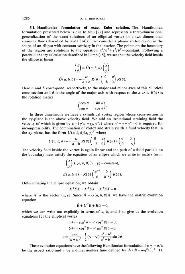
for r small. Thus, -> y + y’ as r- 0. In a similar fashion, we see that 3- 0 as r-> 0.The phase portrait (Fig. 5.2) for the real time formulation has a much simpler

form than that of the Hamiltonian one we first introduced (Fig. 5.1). We see that for(y + y’)/2to < .15, there is a homoclinic loop with hyperbolic fixed point correspondingto the largest root of er(er-1)=((y+’y’)/2to)(e:Zr+l)(er+l). We see that thebifurcation at 3,/to .1227 is represented by the loop crossing the origin.

5.3. Periodic stretching of an elliptical vortex. In general, our perturbed systemwill have the form

f Co cos q + eg(r, q, t),

2tOoer e2 + 1(o

(er + 1)2 Co e2----_1 sin o + eg(r, q, t).

Here g and g are periodic in time, Co (3,o + Y).For 0<Co/tOo<0.15, the unperturbed system has a hyperbolic fixed point

Po at q r/2, r=ro where ro corresponds to the largest real root of the cubice3r+e2r(1-B)+er(l+B)+l=O where B (1/2Cotoo) -1. This fixed point has a homo-clinic saddle connection Fo as depicted in Fig. 5.2. If we consider a perturbationinvolving a periodic stretching by an amount ey"(t), then our perturbation has the form

g- Cl(t) cos

2C2( t)e e2r+lg2

(e + 1)------Cl(t) e2r_ 1sin

Here C1 and C2 are periodic in time with period T. We consider the symmetric casewhere the oscillation of y" puts equal and opposite oscillations on y’ and y while

1290 A.L. BERTOZZI

maintaining the incompressibility condition 3"- 3’ + 3"" 0. Thus, 3’ + 3" stays constanteven though 3’- 3" oscillates with 3’". This implies Cl(t)= 0 so that our perturbationhas the simpler form

2C2(t)egl =0, g2

(e + 1)2.

If we parameterize Fo by (r(t), (t)), the Melnikov function for the perturbed systemcan be calculated using the non-Hamiltonian form. There are two ways of doing theMelnikov function calculation. We can view Fo as a trajectory in the (r, ) coordinatesystem, which has the advantage of a simpler formulation. Since these coordinatesbreak up at r 0, we cannot treat the case where Fo contains the point r 0. Thisoccurs only at the value 3,/to .1227. For any other value of ),/to, we can find a Cvector field (fl (r, ), f2(r, )) so that

f=fl(r, tp), b =f2(r, )is a planar differentiable dynamical system in the coordinates (r, ) with a saddleconnection identical to Fo in its real time parameterization. We have f Co cos ,f2 2tooe/(e + 1)2 Co sin (e2 + 1)/(e2r 1) in a neighborhood of the curve Fo. Thisnew dynamical system is suitable for Melnikov’s method and in a neighborhood of Fohas dynamics identical to that of the original system.

Alternatively, we can treat the evolution equation as a dynamical system in the(x, y) coordinates. This allows us to show that chaos will also occur in the degeneratecase of T/to .1227. Both calculations are presented.

The Melnikov function in (r, ) coordinates. For this we need to knowexp ( tr Df(Fo(s)) ds). We have

e2r + 1 -f(e2r + 1tr Df -Co e2r--’_ COS q9

e2r- 1

This gives us

exp tr Df(ro(s)) dser(t(e"- e-r)

e2r(t)- 1

This yields a Melnikov function

f

_e2r cos q9

M(to) C3 (e A- 1)2(e2r- 1)C2( + to) dt,

C3 Co( ero- e-o).

Using the fact that the integral represents a convolution with an odd function, forC2 cos kt, we have

f

_e2r COS q9

M(to) C3 sin kto (e A- 1)2(e2r 1)sin kt dt

sin ktoMo(k).Since cos p c t:(t), we can see that the above integral is the sine transform of an Lfunction.

e2r cos q9

(er+l)2(e2r--1)dt=2 fo e2r cos

(er+l)2(e2r--1)dt

C3 f r(c3) e2rCo dr(O) er A" 1)2(e2r- 1)

dr< o.


We know by the properties of the Fourier transform on LI(R) ([13, pp. 120-131]) thatM0(k) is a uniformly continuous function of k that is not identically zero. Thus thereexists some interval kl =< k =< k2 such that Mo(k) is nonzero. For these values of k,M(to) has simple zeros.

The Melnikovfunction in (x, y) coordinates. We now consider the dynamical system

2wr sin qer=(y+y’)cos2q-

(er+l)2

e2r + 1+ (y + y’) r sin2 , r 0,

e2r- 1

(3’ + Y’) cos sin q +2wr cos qge e2r + 1

(er+ 1)2(y + y’) .e2.r_ 1

r sin q cos q, r0,

i=y+y’, p=0,

for r=0. Here r=x/x2+y2, =tan-(y/x). We have the time-periodic perturbation

eC2( t)rer (-sin qIif(t, x, y):i cos q/"

The following analysis is for the case y+ y’=.1227; the nondegenerate case can bestudied in a similar fashion. We have

re )f^g=(y+y’)coscpC2(to) (e;])21

tr Df= (3, + Y’) cose2r d- 1)e2r 1

r 0,

=0, r=0,

eJ tr Dfds 2 r(t) e r(

e2r(t)- 1

For C2(t) cos kt, our Melnikov function is

M( to) fo sin kto( t) sin ktr2e2r

(e2-l)(er+l)2dt

sin ktoMo(k).

Again we see that Mo(k) is a sine transform of an L function"

i.(t)r2e2r

(e2- 1)(e+ 1)2r(oo) r2e2r

dt=r(o) (e2- 1)(e + 1)2

dr

(oo) r2 e2r(e2r- 1)(e + 1)2

dr

This is because r2e2r/(e2r--1)(er+ 1)2 is bounded on the interval (0, r(c)]. We seethat Mo(k) is again the sine transform of an odd L function so that there exists aninterval kl <-- k <_- k2 so that Mo(k) is nonzero, giving us a Melnikov function with simplezeros.

1292 A.L. BERTOZZI

Under such a periodic stretching, we find chaotic dynamics occurring in the phaseportrait of the evolution equations for the ellipse. This indicates a sort of randomnessin the evolution of the vortex. The phase portrait includes a horseshoe as a subsystemthat, as we know from 2, indicates somewhat erratic behavior on an invariant set.Assuming the inability to make completely precise measurements, we can only predictwhat will happen to the vortex for a finite time; after this time we have no knowledgeof how it will evolve.

Appendix A. We present the details of the calculation of the following integralfrom 3 via residues"

f -o e/t e-/tMo(K)

(eV, + + e_Vt)2 sin kt tit,

which by a change of variables z yt becomes

y (e --)2 sin mz dr,

where m k y. Consider the meromorphic function

e3z eZ)e imz

(e2Z-e+l)2"The denominator has roots

which we can write as

-e

since we know that 0</3 <2. Here, a =cos-1 (fl/2), which gives us 0< a < r/2. Thus,the function

(e3Z_eZ)e,.,(eZ_e")2(eZ_e-i,)2

has double poles at z +ia +2,a’iN, N 7/. Let r= z-(ia +2,n’iN). The integral isclearly odd in m. Thus we need only consider the case rn > 0. We have that

1 f e3r- eIm J ei, dr

y (e2+fle+l)2

lira ImI [(2N+l) e3 e

r-oo Y a-(2N+l), (e2 + fie + 1)2ei’" d’r

[ ( e3z-ez )lim Im1 1

Res imz- 3, 27ri 0<y<(2N+l)’n" (e2 + fie + 1)2e

e3’ e im,r

zl=(2N+l)r,y>O (e2r-l-/3e + 1)2e dr

The last integral goes to zero as N--> oo so that for m > 0, we wish to calculate

[2,rri (e3::-e )]Im Res(e2 )2

eim3’ y>o + fie + 1


Thus we need to calculate the residues of the function in the upper half-plane. Wecan calculate the coefficients of the Laurent expansion of the function by first consider-ing the expansion of its components in the neighborhood of ia +27tiN. Writingr z (ia + 27riN), we have

e3z eTM 1 + 3r +- +..

eZ= ei (l + r+l- r2+ ")2

r2 +eZ e - 1 + imr2

(e ei)2= e2i(r + r +...),

(e-e-")2= -4 sin2 a +4i sin aesir+ ..We write the function in the form

r c + dr +which has the Laurent expansion

-r + r- +...,C

so that the residue at r 0 is b/c da/c. Here

a (eTM ei)e--,b e--[im(e3i ei) +3e3i

c ei(-4 sin ),

d e (4ie sin 4 sin ).

Let R denote the residue at the point x. Then,--2mN

ei+2iN2 sin

R-2NmNotice that R+- A similar calculation shows that-2mN

R_i+2iN2 sin a

We add the residues in the upper half plane to obtain M(m) for m > 0, and exploitthe fact that M(m) is odd in m to obtain M(m) for m <0. Thus for m 0, ourintegral becomes

M(m)=--2[me-’l msinhlm e-11 ]2 sin sin 1- e-11

elegets. I would like to credit Prof. Andrew Majda of PrincetonUniversity for originally suggesting the idea of extending the Melnikov theory to studythe onset of chaos in fluid flows with heteroclinic orbits. I would also like to thankhim for the guidance he has given me on my A.B. thesis, from which this paper stems.I would like to thank AT&T Bell Laboratories at Murray Hill, New Jersey, where Ispent the summers of 1987 and 1988, for supplying me with the diagrams.

1294 A.L. BERTOZZI

REFERENCES

1] L. V. AHLFORS, Complex Analysis, McGraw-Hill, New York, 1979.[2] V. I. ARNOLD, Mathematical Methods of Classical Mechanics, Springer-Verlag, New York, 1984.[3] V. I. ARNOLD AND A. AVEZ, Ergodic Problems of Classical Mechanics, W. A. Benjamin, New York,

Amsterdam, 1968.[4] A. L. BERTOZZI, An extension ofthe Smale-Birkhoffhomoclinic theorem, Melnikov" method, and chaotic

dynamics in incompressible fluids, A.B. thesis, Princeton University, Princeton, NJ, 1987.[5] G. D. BIRKHOFF, Nouvelles recherches sur les systb.mes dynamiques, Mem. Pont Acad. Sci. Novi Lyncaei,

(1935), pp. 85-216.[6] A.J. CHORIN AND J. E. MARSDEN, A Mathematical Introduction to Fluid Mechanics, Springer-Verlag,

New York, 1979.[7] J. GUCKENHEIMER, A Brief Introduction to Dynamical Systems, Lectures in Applied Mathematics 17,

Springer-Verlag, Berlin, New York, 1979, pp. 187-252.[8] J. GUCKENHEIMER AND P. HOLMES, Nonlinear Oscillations, Dynamical Systems, and Bifurcations of

Vector Fields, Springer-Verlag, New York, 1983.[9] M. W. HIRSCH AND S. SMALL, Differential Equations, Dynamical Systems, and Linear Algebra,

Academic Press, New York, 1974.[10] P. J. HOLMES, Averaging and chaotic motions in forced oscillations, SIAM J. Appl. Math., 38 (1980),

pp. 68-80.[11] "’Space and Time Periodic Perturbations of the sine-Gordon Equation, in Dynamical Systems

and Turbulence, D. A. Rand and L.-S. Young, eds., Lecture Notes in Mathematics 89, Springer-Verlag, New York, Berlin, 1981.

[12] HOLM, MARSDEN, AND RATIU, Nonlinear stability of the Kelvin-Stuart cat’s eyesflow, in AMS Proc.Math. BiD. Symposia and Summer Seminars, July, 1979.

[13] Y. KATZNELSON, An Introduction to Harmonic Analysis, Dover, New York, 1976.[14] S. KIDA, J. Phys. Soc. Japan, 50 (1981), pp. 3517-3520.[15] H. LAMB, Hydrodynamics, Dover, New York, 1945.[16] A. MAJDA, Lectures on Incompressible Fluid Flow-Fall 1986, Princeton, NJ, 1986.[17] J. E. MARSDEN, Chaotic orbits by Melnikov’s method: a survey of applications, PAM-173/COMM,

Center for Pure and Applied Mathematics, University of California, Berkeley, CA, August 1983.[18] V. K. MELNIKOV, On the stability of the center for time periodic perturbations, Trans. Moscow Math.

Soc., 12 (1963), pp. 1-57.[19] J. MOSER, Stable and Random Motions in Dynamical Systems, Princeton University Press, Princeton,

NJ, 1973.[20] D. W. MOORE AND P. G. SAFFMAN, The density of organized vortices in a turbulent mixing layer,

J. Fluid Mech., 69 (1975), pp. 465-473.[21] J. C. NEU, The Dynamics of a Columnar Vortex in an Imposed Strain, MRSI 022-83, 1983.[22] ., The dynamics of stretched vortices, J. Fluid Mech., 143 (1984), pp. 253-276.[23] J. PALLS, On Morse-Smale dynamical systems, Topology, 8 (1969), pp. 385-405.[24] J. PEDLOSKY, Geophysical Fluid Dynamics, Springer-Verlag, New York, 1982.[25] A. P. PRUDNIKOV, Y. A. BRYCHKOV, AND O. I. MARICHEV, Integrals and Series: Vol. I. Elementary

Functions (translated from Russian by N. M. Queen) Gordon and Breach, New York, 1986.[26] S. SMALL, Differomorphisms with many periodic points, in Differential and Combinatorial Topology,

S. S. Cairns, ed., Princeton University Press, Princeton, NJ, 1963, pp. 63-80.[27] J. T. STUART, Stability Problems in Fluids, AMS Lectures in Applied Mathematics 13, American

Mathematical Society, Providence, RI, 1971, pp. 139-155.

siam math. anal. vol. no. - ucla department of …bertozzi/papers/sima88.pdf · · 2011-03-07siam...

Documents