signal analysis in guided wave structural health
TRANSCRIPT

SIGNAL ANALYSIS IN GUIDED WAVE STRUCTURAL HEALTHMONITORING
By
Oleksii Karpenko
A THESIS
Submitted toMichigan State University
in partial fulfillment of the requirementsfor the degree of
Electrical Engineering - Master of Science
2013

ABSTRACT
SIGNAL ANALYSIS IN GUIDED WAVE STRUCTURAL HEALTHMONITORING
By
Oleksii Karpenko
In recent decades, Guided waves (GW) have emerged as the most promising modality for
Structural Health Monitoring (SHM). In SHM applications with distributed sensor networks,
GWs can be efficiently actuated with the help of surface-bonded or embedded piezoelectric
elements. Nevertheless, the analysis of GW signals and accurate identification of damage
sites still remains a challenge. Algorithms for locating defects, such as Probability Diagnostic
Imaging, usually assume unimodal GW propagation. However, in many cases selective mode
excitation could be hardly accomplished in practice. From this perspective, decomposition
of the measured signal into its constituent components is a critical requirement for accurate
damage detection. This work presents a signal processing method that combines time-
frequency representation (TFR) with Matching Pursuit (MP) for decoupling of GW modes.
The proposed TFR is designed on the basis of the reassigned spectrogram whose kernel is
substituted with a Chirp-Z transform in order to improve the resolution without increasing
its computational complexity. The MP dictionary is constructed of atoms, which numerically
simulate the propagation of wave packets corresponding to different GW modes in the sample.
The dictionary also accounts for the effect of bonding between the piezoelectric element and
the structure. Performance of the algorithm is demonstrated on aluminum plates and woven
composite samples for cases when two fundamental modes S0 and A0 are simultaneously
actuated.

TABLE OF CONTENTS
LIST OF TABLES . . . . . . . . . . . . . . . . . . . . . . . . . . . . . . v
LIST OF FIGURES . . . . . . . . . . . . . . . . . . . . . . . . . . . . . . vi
CHAPTER 1 Structural Health Monitoring . . . . . . . . . . . . . . . . . . 11.1 Introduction . . . . . . . . . . . . . . . . . . . . . . . . . . . . . . . . . . . . 11.2 SHM Techniques and Sensing Modalities . . . . . . . . . . . . . . . . . . . . 4
1.2.1 Ultrasonic Testing and Guided Wave SHM . . . . . . . . . . . . . . . 61.3 Guided Wave Theory . . . . . . . . . . . . . . . . . . . . . . . . . . . . . . . 7
1.3.1 Symmetric Solution . . . . . . . . . . . . . . . . . . . . . . . . . . . . 121.3.2 Antisymmetric Solution . . . . . . . . . . . . . . . . . . . . . . . . . 131.3.3 Phase Velocity and Group Velocity Dispersion Curves . . . . . . . . . 141.3.4 Mode Shapes . . . . . . . . . . . . . . . . . . . . . . . . . . . . . . . 161.3.5 Transduction of Guided Waves . . . . . . . . . . . . . . . . . . . . . . 17
1.3.5.1 PZT Wafers and Piezoelectric Governing Equations . . . . . 181.3.5.2 Anisotropic Piezoelectric Transducers . . . . . . . . . . . . . 20
1.4 Actuation of Guided Waves with Surface-bonded Piezoelectric Transducers . 211.4.1 Shear Lag Model . . . . . . . . . . . . . . . . . . . . . . . . . . . . . 211.4.2 Ideal Bonding Assumption . . . . . . . . . . . . . . . . . . . . . . . . 261.4.3 Voltage Output of the PZT Sensor . . . . . . . . . . . . . . . . . . . 28
CHAPTER 2 Signal Analysis in Guided Wave SHM . . . . . . . . . . . . 292.1 Overall Approach to Damage Detection . . . . . . . . . . . . . . . . . . . . . 292.2 Probability Diagnostic Imaging . . . . . . . . . . . . . . . . . . . . . . . . . 312.3 Challenges in Signal Processing of Guided Waves . . . . . . . . . . . . . . . 322.4 Characteristic Features for Mode Identification . . . . . . . . . . . . . . . . . 342.5 Time-Frequency Representations in GW SHM . . . . . . . . . . . . . . . . . 35
2.5.1 Linear Time-Frequency Representations . . . . . . . . . . . . . . . . 362.5.1.1 Short Time Fourier Transform . . . . . . . . . . . . . . . . . 362.5.1.2 Continuous Wavelet Transform . . . . . . . . . . . . . . . . 392.5.1.3 Chirplet Transform and Warping Operators . . . . . . . . . 40
2.5.2 Quadratic TFRs . . . . . . . . . . . . . . . . . . . . . . . . . . . . . 422.5.2.1 Wigner-Ville Distribution . . . . . . . . . . . . . . . . . . . 43
2.5.3 Time-Frequency Reassignment . . . . . . . . . . . . . . . . . . . . . . 44
iii

2.6 Reassigned Spectrogram with Chirp Transform Kernel . . . . . . . . . . . . 472.7 Matching Pursuit (MP) algorithms in Guided wave signal processing . . . . 53
2.7.1 Gabor, Chirplet and Dispersion-based Dictionaries for MP . . . . . . 542.7.2 Generation of Atoms of the Dispersion-based Dictionary . . . . . . . 55
2.8 Hybrid Algorithm based on RSCT and Matching Pursuit with Dispersion-based Dictionary for Mode Decomposition of Guided Wave Signals . . . . . . 582.8.1 Efficient Implementation of the MD Algorithm . . . . . . . . . . . . . 59
CHAPTER 3 Experimental Studies . . . . . . . . . . . . . . . . . . . . . . . 613.1 Defect Localization in Metal Structures . . . . . . . . . . . . . . . . . . . . . 613.2 Defect Localization in Woven Composite Structures . . . . . . . . . . . . . . 67
CHAPTER 4 Conclusions and Future Work . . . . . . . . . . . . . . . . . 74
APPENDICES . . . . . . . . . . . . . . . . . . . . . . . . . . . . . . . . . . . . . 76Appendix A: Expression of Stresses, Strains and Displacements in terms ofWave Potentials . . . . . . . . . . . . . . . . . . . . . . . . . . . . . . . . . . 77Appendix B: Relationship between Stiffness Constants, Young’s Moduli andPoisson’s Ratios for Orthotropic Materials . . . . . . . . . . . . . . . . . . . 79
BIBLIOGRAPHY . . . . . . . . . . . . . . . . . . . . . . . . . . . . . . . . . . . 81
iv

LIST OF TABLES
Table 3.1 Length of possible wave paths and corresponding Times-of-Flight forS0 and A0 modes. . . . . . . . . . . . . . . . . . . . . . . . . . . . . 65
Table 3.2 Comparison of analytic and MD-extracted Times-of-Flight for S0 andA0 modes. . . . . . . . . . . . . . . . . . . . . . . . . . . . . . . . . 65
v
LIST OF FIGURES
Figure 1.1 SHM with distributed sensor networks. Overall approach and mainstages [2]. For interpretation of the references to color in this and allother figures, the reader is referred to the electronic version of thisthesis. . . . . . . . . . . . . . . . . . . . . . . . . . . . . . . . . . . . 3
Figure 1.2 Shear vertical and pressure waves in solids. . . . . . . . . . . . . . . 10
Figure 1.3 Isotropic plate of infinite length and thickness 2d. Wave propagatesin x-direction. . . . . . . . . . . . . . . . . . . . . . . . . . . . . . . 10
Figure 1.4 Phase velocity dispersion curves of 2-mm thick aluminum plate. . . 15
Figure 1.5 Group velocity dispersion curves of 2-mm thick aluminum plate. . . 15
Figure 1.6 Displacements of S0 mode. . . . . . . . . . . . . . . . . . . . . . . . 16
Figure 1.7 Displacements of A0 mode. . . . . . . . . . . . . . . . . . . . . . . . 17
Figure 1.8 Transducers for actuation and sensing of Guided waves. . . . . . . . 18
Figure 1.9 Piezoelectric effect: a).neutral state; b). strain conversion; c). voltageconversion. . . . . . . . . . . . . . . . . . . . . . . . . . . . . . . . . 19
Figure 1.10 Anisotropic Piezocomposite Transducers. . . . . . . . . . . . . . . . 21
Figure 1.11 Actuation using surface-bonded PZT. . . . . . . . . . . . . . . . . . 22
Figure 1.12 Actuation using collocated PZT pairs. . . . . . . . . . . . . . . . . . 23
Figure 1.13 Shear lag model: surface stress. . . . . . . . . . . . . . . . . . . . . 25
Figure 1.14 Shear lag model: surface strain. . . . . . . . . . . . . . . . . . . . . 25
vi

Figure 1.15 Actuation using surface-bonded PZT. . . . . . . . . . . . . . . . . . 27
Figure 2.1 PZT sensor configurations. . . . . . . . . . . . . . . . . . . . . . . . 30
Figure 2.2 Approach to signal processing. . . . . . . . . . . . . . . . . . . . . . 33
Figure 2.3 Narrowband actuation waveform. . . . . . . . . . . . . . . . . . . . 34
Figure 2.4 Dispersion curves of a 2-mm thick aluminum plate corresponding tothe spectrum of the Morlet wavelet. . . . . . . . . . . . . . . . . . . 35
Figure 2.5 Time-frequency tiling of STFT. . . . . . . . . . . . . . . . . . . . . 38
Figure 2.6 Time-frequency tiling using dyadic wavelets. . . . . . . . . . . . . . 39
Figure 2.7 Warped tiling of time-frequency plane. . . . . . . . . . . . . . . . . . 41
Figure 2.8 Ideal TFR and Wigner-Ville distribution of the signal. . . . . . . . . 45
Figure 2.9 Comparison of smoothed WVD and STFT of the signal (windowlength = 413 points). . . . . . . . . . . . . . . . . . . . . . . . . . . 46
Figure 2.10 Comparison of reassigned smoothed WVD and reassigned spectro-gram of the signal (window length = 413 points). . . . . . . . . . . . 46
Figure 2.11 Comparison of Discrete Fourier transform with Chirp-Z transform. . 50
Figure 2.12 Implementation of Chirp-Z transform algorithm. . . . . . . . . . . . 50
Figure 2.13 Experimental set-up for obtaining GW signal: 600×600×2 mm alu-minum plate. . . . . . . . . . . . . . . . . . . . . . . . . . . . . . . . 51
Figure 2.14 FFT of GW signal. . . . . . . . . . . . . . . . . . . . . . . . . . . . 51
Figure 2.15 CZT of GW signal. Zooming into 220-320 kHz range. . . . . . . . . 51
Figure 2.16 Lamb wave signal (10240 samples). . . . . . . . . . . . . . . . . . . 52
Figure 2.17 STFT (window size 350 samples). . . . . . . . . . . . . . . . . . . . 52
vii

Figure 2.18 Reassigned spectrogram with CZT. . . . . . . . . . . . . . . . . . . 52
Figure 2.19 Atoms of conventional MP dictionaries: Gabor and two chirplets withdifferent scales. . . . . . . . . . . . . . . . . . . . . . . . . . . . . . . 55
Figure 2.20 Generated atoms of A0 mode propagating in 2 mm thick aluminumplate at 0.25 m, 0.5 m, 1.0 m and 1.5 m from the actuator. Actuationwaveform: 250 kHz, 5 cycle Hann windowed sinusoid. . . . . . . . . 56
Figure 2.21 Influence of PZT strain transfer conditions on the actuated GW modes. 57
Figure 2.22 Spectra of S0 and A0 modes generated by surface-bonded PZT. . . . 57
Figure 2.23 Flowchart of the two stage MD algorithm. . . . . . . . . . . . . . . . 58
Figure 3.1 Experimental set-up for damage detection in aluminum plates. . . . 62
Figure 3.2 Group velocity dispersion curves of the aluminum plate used in theexperiment. . . . . . . . . . . . . . . . . . . . . . . . . . . . . . . . 62
Figure 3.3 Possible wave paths from the actuator to the receiving PZT. . . . . 63
Figure 3.4 GW actuation using single surface-bonded PZT-1. . . . . . . . . . . 63
Figure 3.5 Reassigned spectrogram with CZT. . . . . . . . . . . . . . . . . . . 63
Figure 3.6 Collocated actuation of Guided waves. . . . . . . . . . . . . . . . . . 63
Figure 3.7 MD decomposed A0 components. . . . . . . . . . . . . . . . . . . . 64
Figure 3.8 MD decomposed S0 components. . . . . . . . . . . . . . . . . . . . . 64
Figure 3.9 MD decomposed shear wave components. . . . . . . . . . . . . . . . 64
Figure 3.10 Damage detection in 2-mm thick aluminum plate. . . . . . . . . . . 66
Figure 3.11 Signal from PZT 1-2 sensor pair. . . . . . . . . . . . . . . . . . . . . 66
Figure 3.12 Signal from PZT 2-3 sensor pair. . . . . . . . . . . . . . . . . . . . . 66
viii

Figure 3.13 Phase velocity dispersion curves generated for 5-mm thick 8-layercomposite plate with the help of Transfer Matrix method. . . . . . . 69
Figure 3.14 Damage detection in 2-mm thick aluminum plate. . . . . . . . . . . 70
Figure 3.15 Variation of the group velocity of A0 mode actuated at 70 kHz withrespect to the direction of propagation in a 5-mm thick 8-layer wovencomposite plate. . . . . . . . . . . . . . . . . . . . . . . . . . . . . . 71
Figure 3.16 Composite samples used in experimental studies. . . . . . . . . . . . 72
Figure 3.17 Probability Diagnostic Imaging on composite samples. . . . . . . . . 72
Figure 3.18 Baseline and differenced signal obtained by PZT-6 and PZT-2 sensorpair on composite plate. . . . . . . . . . . . . . . . . . . . . . . . . . 72
ix

CHAPTER 1
Structural Health Monitoring
1.1 Introduction
In recent years, there has been an increasing demand for methods providing in-situ Struc-
tural Health Monitoring (SHM) of safety-critical systems. Numerous disastrous events such
as disintegration of space shuttle Challenger (Canaveral National Seashore, 1986), San Bruno
pipeline explosion (California, 2006), Hoan Bridge failure (Wisconsin, 2001) and various
flight accidents [1] caused by undetected structural defects, have increased public concerns
about the need for more reliable NDE methods. Current industrial practice involves well-
established techniques such as eddy current, optical and ultrasonic testing due to their ability
to furnish precise information about structural damage, its location and severity. However,
these NDE inspections are required at scheduled intervals to assess the integrity of a compo-
nent during its downtime. Moreover, it is always possible that damage might occur in service
and maintenance schedules will not be adequate to detect an impending hazard. From this
perspective, the transition from regular maintenance to condition-based maintenance is envi-
1

sioned as an efficient solution to minimizing catastrophic failures of safety-critical structures.
In Chapter 1 we consider main concepts of Structural Heath Monitoring and present
a brief overview of sensing modalities used in modern SHM. Chapter 1 also describes the
key elements and operation of GW monitoring systems, which interrogate the structure
with piezoelectric transducers. Additionally, we provide the essential background for solving
problems in Guided wave signal analysis, such as Rayleigh-Lamb equations governing the
propagation of Guided waves in plates and a theory of GW actuation with the help of
surface-bonded wafers.
Structural Health Monitoring can be viewed as an efficient approach to continual diag-
nostics of complex structures with the help of structurally integrated sensor networks. SHM
is initially aimed at detecting damage and degradation of constituent materials caused by
sudden or dynamic stresses or respectively, fatigue, corrosion and environmental changes
experienced by the structure in service. However, its global objective is to provide a com-
prehensive estimate of structural integrity as well as to generate data required for statistical
analysis and long term prognosis.
Schematic of a typical SHM application is demonstrated in Fig. 1.1. In a monitoring
system, sensors can be strategically placed (embedded or surface-mounted) in the critical
areas of the structure in order to collect signals which would be informative enough for dam-
age detection. Hardware components of the system also include autonomous low footprint
devices or sensor nodes designed to control the data acquisition process and to transmit
the data to remotely installed base station. Base station is usually a personal computer
that supports real-time signal processing applications. The purpose of signal analysis is the
extraction of characteristic features from the acquired signals, which helps locate damaged
2

Figure 1.1: SHM with distributed sensor networks. Overall approach and main stages [2].For interpretation of the references to color in this and all other figures, the reader is referredto the electronic version of this thesis.
sites and classify detected defects. It should be noted that modern SHM applications also
take advantage of wireless data transmission and therefore, they additionally require devel-
opment of specialized communication protocols that would enable reliable data transfer and
realization of different network topologies. Finally, SHM systems may store baselines, mate-
rial databases and threshold values in order to establish an accurate damage identification
criterion. Clearly, SHM technology has many advantages and it offers a great potential to
overcome the shortcomings of conventional NDE methods. Firstly, preventive damage detec-
tion provides an early warning and allows for the immediate repair in order to prolong the
lifespan of structural components. Secondly, continual monitoring is cost-efficient because it
reduces the downtime of the system.
3

1.2 SHM Techniques and Sensing Modalities
The analysis of recent works on SHM shows that various sensing schemes can be efficiently
employed in a monitoring system. However, the selection of a sensing modality highly
depends on a particular industrial application. Generally, sensing methods in SHM can be
broadly classified as passive and active depending on the actuation capabilities of the system.
Passive sensing accrues information about the current state of the structure from its
vibrations or deformation under stress. Such an approach to data acquisition enables the
implementation of many damage detection techniques based on mode shape, mode curvature,
impedance or Fourier analysis. For instance, UT sensors can be used for continual monitoring
of helicopter engine shafts: if defect occurs the resonant frequencies of the collected signals
may change significantly [10]. One more example of a passive sensing technique is Acoustic
Emission (AE). Recently, the use of AE-based SHM systems has been reported in nuclear
power industry [11]. Usually, AE sensors are strategically placed in safety-critical areas of the
plant; the sensors stay in idle mode and continuously ”listen” to possible acoustic signatures
emitted by newly appearing defects. Another growing trend in passive techniques is the
increasing popularity of FBG sensors for SHM of composite materials. Minimal FBG strain
causes the spectrum of light passing through it to shift or attenuate in frequency domain. And
since composites are susceptible to matrix cracking and delamination between the layers, the
high sensitivity of FBGs to minor deviations of strain in damaged areas is crucial for reliable
defect detection. However, despite the simplicity of data analysis, all passive methods share
one major drawback − their sensors have a very local range meaning that if damage occurs
at some distance, it will never be detected. Therefore, such SHM systems require large
density of receivers per unit area, which in turn increases the number of acquisition nodes
4

and conditioning circuits. As a consequence, passive sensing is generally worth implementing
for monitoring of the most failure-prone components such as dynamically loaded structures,
cohesively bonded or riveted elements, composite stiffeners, surfaces subjected to impacts,
etc. But whenever passive techniques are used for large-scale applications, some defects can
be missed and only a “global” assessment can be obtained. This is due to the sparsity of
sensor arrays, which limits the area of coverage.
Unlike passive methods, active modalities utilize the actuators to perturb the structure
and examine it at any desired time. Therefore, it is always possible to perform an automatic
inspection in repeatable manner that follows a maintenance schedule. Moreover, critical
areas can be scanned locally if necessary, since active SHM systems provide full control of
their excitation sources. Depending on damage detection scheme, actuators can be excited
in groups or sequentially in order to interrogate the region of interest. Then the response
is measured by sensors and processed by signal processing software. Data corresponding to
current and previous states of the structure are often compared to identify damage presence,
its location and severity. It is worth mentioning that conventional NDE incorporates many
active methods, such as radiography, eddy current, microwave tomography, thermo-optical
scans, etc.; but only few of them can be efficiently adopted in SHM applications. This is due
to a number of design constraints, the most important of which is the need for small and
lightweight transducers driven by compact devices with on-board processor. In addition,
the whole system should be low cost and have the capability of being easily deployed on
the structure. From this perspective, the technologies showing most amount of promise for
active SHM belong to the field of ultrasonics.
5

1.2.1 Ultrasonic Testing and Guided Wave SHM
Active ultrasonic methods can be broken down into bulk wave inspection and guided
waves. Unfortunately, bulk wave NDE have shown to be somewhat impractical for SHM
purposes, since it involves the use of wedge-mounted transducers with grease couplants.
Moreover, it requires a tedious data collection procedure: bulk waves are excited by surface
“tapping” and propagate through the thickness of the structure providing only point-by-point
measurements.
In contrast to bulk waves, Guided wave inspection has recently emerged as a prominent
modality that is easily transitioned to SHM systems. Guided waves are elastic waves that
follow the boundaries of the media in which they propagate. The main advantage of GWs
is their ability to travel long distances without high energy losses, which provides large area
coverage of the components to be monitored. The capability of GWs to penetrate through
the thickness of the structure makes them sensitive to different imperfections such as cracks,
impact damage and delaminations, essential in real-time SHM.
Guided waves exist in waveguides whose one particular dimension is much smaller than
the others. The simplest examples of such geometries would include rods, plates, shells and
pipes. If the wavelength is bigger than the thickness of the structure, a guided wave is con-
fined between the boundaries through multiple reflections and propagates with complicated
particle displacement patterns. GWs can be excited in many possible modes having different
velocity and shape. Hence, the selection of the appropriate mode is important for maximiz-
ing damage detection capabilities of the system. Next section presents a brief introduction
to Guided wave theory, since understanding of wave propagation in solids is essential for
solving problems of GW signal analysis.
6
1.3 Guided Wave Theory
Guided wave theory dates back to the beginning of the twentieth century, when the
main concepts of elastic wave propagation in solids were studied by Horace Lamb [12]. The
British mathematician was the first to explain special properties of waves propagating in
plates of infinite extent. Consequently, guided waves have been also called Lamb waves. In
1967, Viktorov used programmed digital device to analyze Lamb’s equations and generate
the dispersion curves: the non-linear relationship between the wave speed and actuation
frequency for different propagation modes. Later he published his comprehensive study of
GWs in isotropic plates highlighting their potential for NDE [13].
However, the truly broad use of guided waves in numerous applications was inspired by
the advent of computer era. The advantage of high computational power opened the oppor-
tunity to implement guided wave technology for the inspection of structures with complex
geometries and materials. It also facilitated the development of finite element modeling and
signal processing algorithms for wave propagation analysis and damage detection. Works
having the highest impact on guided wave NDE and SHM were reported by Rose, Nayfeh,
Graff, Alleyne and many others [14, 15, 16].
This section introduces the fundamental equations describing Guided waves in isotropic
plate-like structures. Since the topic is well documented in the literature, only the key results
are presented in this section and the intermediate steps are summarized in the Appendix A.
The case of fiber-reinforced composites is outlined in Chapter 3.
The constitutive relations describing Guided waves in plates can be thought of as a special
case of elastic wave propagation in unbounded media. The differential equation of motion
7

in three-dimensional solids is known as Navier’s equation [17]:
µ( ∂
∂x2 + ∂
∂y2 + ∂
∂z2 )ux+ (λ+µ) ∂∂x
( ∂∂x
+ ∂
∂y+ ∂
∂z)ux = ρ
∂ux
∂t2
µ( ∂
∂x2 + ∂
∂y2 + ∂
∂z2 )uy+ (λ+µ) ∂∂x
( ∂∂x
+ ∂
∂y+ ∂
∂z)uy = ρ
∂uy
∂t2
µ( ∂
∂x2 + ∂
∂y2 + ∂
∂z2 )uz + (λ+µ) ∂∂x
( ∂∂x
+ ∂
∂y+ ∂
∂z)uz = ρ
∂uz
∂t2
(1.1)
Eq. (1.1) can be concisely expressed in vector form:
µ∇2u + (λ+µ)∇(∇·u) = ρ∂u∂t2
(1.2)
where u = iux+ juy+ kuz is the particle displacement vector, ρ is the material density, µ and
λ are the Lame constants, the ∇ is a del differential operator and ∇2 is a vector Laplacian.
It should be noted that Navier’s differential equations governing wave propagation are
based upon three fundamental relationships from linear elasticity theory. These include
strain-displacement relations (Eq. (1.3)), equation of motion also known as Newton’s general-
ized second law (Eq. (1.4)) and constitutive stress-strain relations or Hooke’s law (Eq. (1.5)).
Their expressions in tensor notation are:
εij = 12(uj,i+ui,j) (1.3)
∂σij∂xi
= ρ∂ui∂t2
(1.4)
σij = cijklεkl(1.5)
where i, j = 1,2,3; εij − the strain tensor and cijkl − the stiffness tensor; repeated in-
8

dexes imply summations and commas imply partial derivatives. Therefore, Navier’s equation
combines three equilibrium equations, six strain-displacement equations, and six constitu-
tive equations from Eq. (1.3)−Eq. (1.5). Navier’s equation can be solved with the help of
Helmholtz vector and scalar potentials H and Φ :
u =∇Φ +∇×H (1.6)
∇·H = 0 (1.7)
Upon the substitution of Eq. (1.5) and Eq. (1.6) into Eq. (1.1) we get
(λ+ 2µ)∇2Φ−ρ∇Φ = 0 (1.8)
µ∇2H−ρH = 0 (1.9)
The rearrangement of (1.8-1.9) yields the equation of wave propagation in 3D homogeneous
solids in terms of scalar and vector potentials
cl2∇2Φ= Φ
cs2∇2H = H
(1.10)
where cl = (2µ+λ)/ρ and cs = µ/ρ. Double dot operator represents the second order time
derivative. It can be shown that the total solution for displacement vector u has three
components [17]:
u = uL + uSH + uSV (1.11)
9

where uL corresponds to longitudinal or pressure wave whose particle displacement is parallel
to the direction of propagation, uSH and uSV define the shear horizontal and shear vertical
waves. Motion of particles for these solutions is perpendicular to the direction of wave
propagation. The snapshots of S-wave and P-wave are shown in Fig. 1.2.
Figure 1.2: Shear vertical and pressure waves in solids.
Shear vertical and pressure wave solutions are of particular importance if Navier’s equa-
tions are solved for practical cases when the structure has some geometric bounds. In
particular, the interaction of shear vertical and pressure waves in thin plates and shells gives
rise to guided waves. In this section we consider the derivation of Lamb wave equations for
two-dimensional plates of infinite length. For simplicity of analysis it is possible to assume
that the wave potentials are invariant to the z-direction along the wave front [17].
Figure 1.3: Isotropic plate of infinite length and thickness 2d. Wave propagates in x-direction.
10
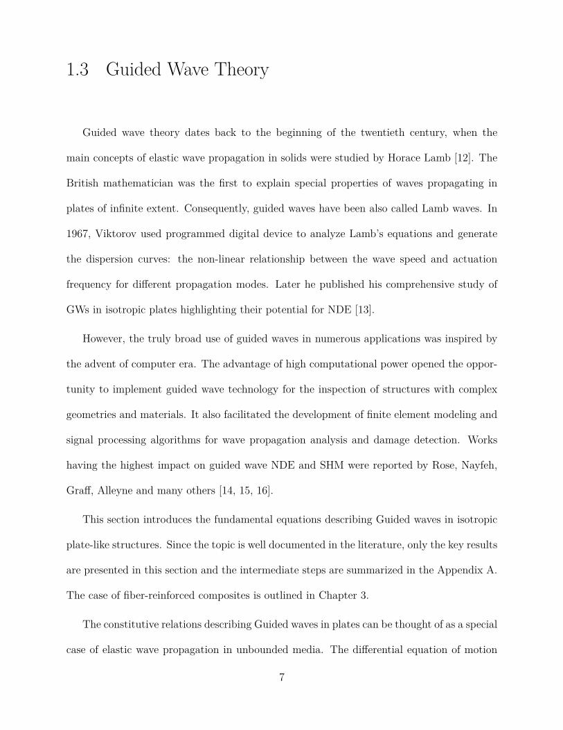
In this case ∂/∂z = 0 and uSH accepts only shear displacement uz . In contrast, uL
with uSV accept ux and uy displacements, which depend only on scalar potential Φ and a
z-component of a vector potential Hz . Therefore, Navier’s equation in terms of scalar and
vector potentials for uL, uSV possible solutions and the geometry in Fig. 1.3 takes the form:
cl
2∇2Φ= Φ
cs2∇2Hz = Hz
(1.12)
where cl and cs are longitudinal and shear wave speeds.
Introducing the simpler notation Φ = φ and Hz = ψ we get a classical formulation for
Lamb wave equations in the potential form:
∂2φ∂x2 + ∂2φ
∂y2 + ω2
cp2φ= 0
∂2ψ∂x2 + ∂2ψ
∂y2 + ω2
cs2ψ = 0(1.13)
Assuming harmonic solution e−i(ωt−ξx), the system of equations Eq. (1.13) becomes:
∂2φ∂y2 + ( ω
2
cp2 − ξ2)φ= 0
∂2ψ∂y2 + ( ω
2
cs2 − ξ2)ψ = 0
(1.14)
In Eq. (1.14), ξ = ω/c defines a wavenumber. At this point we can introduce the more
compact notation for convenience:
p2 = ω2
cp2 − ξ2
q2 = ω2
cs2 − ξ2
(1.15)
11
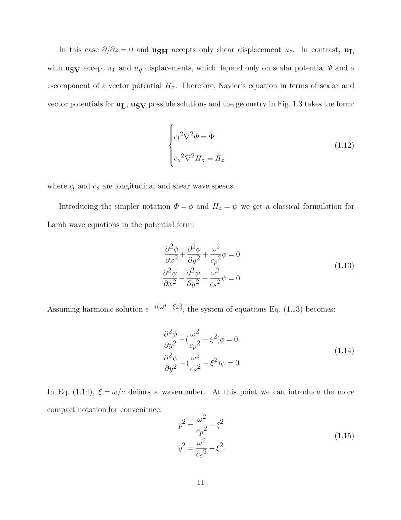
Hence,∂2φ∂y2 +p2φ= 0
∂2ψ∂y2 + q2ψ = 0
(1.16)
The general solution for the above system takes the form:
φ= A1 sinpy+A2 cospy
ψ =B1 sinqy+B2 cosqy(1.17)
where A1, A2, B1 and B2 are constants to be determined from the boundary conditions.
1.3.1 Symmetric Solution
Symmetric solution implies that ux component of the displacement vector and shear
stresses are symmetric about the midplane across the thickness of the plate, namely
ux(x,−d) = ux(x,d)
uy(x,−d) =−uy(x,d)
τyx(x,−d) =−τyx(x,d)
τyy(x,−d) = τyy(x,d)(1.18)
Symmetric boundary conditions also include traction free surfaces
τyx(x,−d) =−τyx(x,d) = 0
τyy(x,−d) = τyy(x,d) = 0(1.19)
12
Using the general solution for potentials in Eq. (1.17) and formulas for displacements and
stresses from the Appendix A, Eq. (1.19) can be expressed as
−2iξA2 sinpd+B1(ξ2− q2)sinqd= 0
A2(ξ2− q2)cospd−2iξB1 cosqd= 0(1.20)
A non-trivial solution for the above linear system of equations exists if the determinant in
Eq. (1.20) vanishes:
MS= (ξ2− q2)2 sinqdcospd+ 4ξ2pq cosqd= 0 (1.21)
Rearranging Eq. (1.21) yields the dispersion relation for symmetric modes:
tanpdtanqd =−(ξ2− q2)2
4ξ2pq(1.22)
where p and q are given in Eq. (1.15).
1.3.2 Antisymmetric Solution
Antisymmetric solution requires that displacements and stresses are antisymmetric with
respect to the midplane
ux(x,−d) =−ux(x,d)
uy(x,−d) = uy(x,d)
τyx(x,−h) = τyx(x,h)
τyy(x,−h) =−τyy(x,h)(1.23)
13

The antisymmetric boundary conditions are the following
τyx(x,−d) = τyx(x,d) = 0
τyy(x,−d) =−τyy(x,d) = 0(1.24)
Using the general solution for the potentials in Eq. (1.17) and formulas for the displacements
and stresses from the Appendix A, Eq. (1.24) can be expressed as
2iξA1 cospd+B2(ξ2− q2)cosqd= 0
A1(ξ2− q2)sinpd+ 2iξB2 cosqd= 0(1.25)
A non-trivial solution exists if determinant in Eq. (1.25) vanishes:
MA= (ξ2− q2)2 sinpdcosqd+ 4ξ2pq cosqdsinqd= 0 (1.26)
Finally, we obtain Lamb wave equation for antisymmetric modes:
tanpdtanqd =− 4ξ2pq
(ξ2− q2)2 (1.27)
It can be noticed that the right-hand side of Eq. (1.22) is reciprocal to that of Eq. (1.27).
1.3.3 Phase Velocity and Group Velocity Dispersion Curves
It can be noticed that solutions of Rayleigh-Lamb equations in Eq. (1.22) and Eq. (1.27)
define the dispersion curves or the relationship between the phase velocity, cph and the
14

actuation frequency, ω. Since p and q also depend on ω, the phase velocity should be
evaluated numerically at each frequency step for a fixed value of a plate thickness 2h.
Figure 1.4: Phase velocity dispersion curves of 2-mm thick aluminum plate.
Figure 1.5: Group velocity dispersion curves of 2-mm thick aluminum plate.
∂c
∂(fd)∼=
∆c∆(fd)
(1.28)
The example of phase velocity dispersion curves is presented in Fig. 1.4. It follows that
the solution is not unique, and at high frequency-thickness products multiple symmetric
and antisymmetric modes exist in the plate. However, the knowledge of group velocity
15

dispersion curves (Fig. 1.5) can be considered even more important, since the group velocity,
cgr determines how fast the wavefront of each mode propagates. This enables one to calculate
the Time-of-Flight (ToF) and distance traveled by wave packets in the structure, which is
essential for locating damage sites. Group velocity dispersion curves can be obtained from
the phase velocity data using the finite difference formula (Eq. (1.28)).
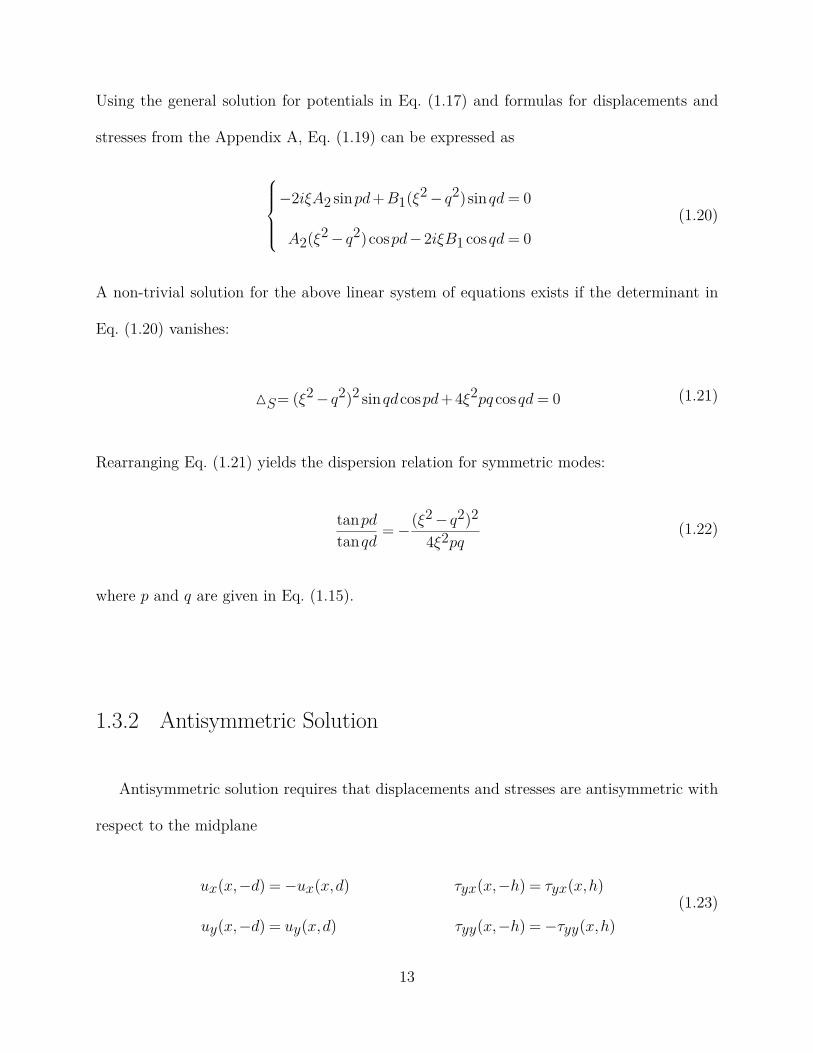
1.3.4 Mode Shapes
The across-thickness particle motion or mode shape can be considered another important
aspect of reliable damage detection in GW SHM. In fact, the mode shape determines the
sensitivity of a particular mode to different defects at some actuation frequency. For ex-
(a) Actuation frequency 1000 kHz (b) Actuation frequency 3000 kHz
Figure 1.6: Displacements of S0 mode.
ample, the dominance of uy component indicates the increased sensitivity to surface defects,
and big displacements ux along the direction of wave propagation provide good sensitivity
to cracks. Fig. 1.6 and Fig. 1.7 illustrate displacement components of S0 and A0 modes that
propagate in 1-mm thick aluminum plate.
16
(a) Actuation frequency 1000 kHz (b) Actuation frequency 3000 kHz
Figure 1.7: Displacements of A0 mode.
1.3.5 Transduction of Guided Waves
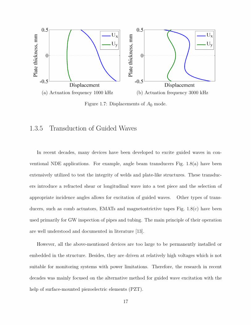
In recent decades, many devices have been developed to excite guided waves in con-
ventional NDE applications. For example, angle beam transducers Fig. 1.8(a) have been
extensively utilized to test the integrity of welds and plate-like structures. These transduc-
ers introduce a refracted shear or longitudinal wave into a test piece and the selection of
appropriate incidence angles allows for excitation of guided waves. Other types of trans-
ducers, such as comb actuators, EMATs and magnetostrictive tapes Fig. 1.8(c) have been
used primarily for GW inspection of pipes and tubing. The main principle of their operation
are well understood and documented in literature [13].
However, all the above-mentioned devices are too large to be permanently installed or
embedded in the structure. Besides, they are driven at relatively high voltages which is not
suitable for monitoring systems with power limitations. Therefore, the research in recent
decades was mainly focused on the alternative method for guided wave excitation with the
help of surface-mounted piezoelectric elements (PZT).
17
(a) Wedge transducer [18]. (b) Comb transducer [19].
(c) Magnetostricitive trans-ducer [19].
(d) PZT wafer [20].
Figure 1.8: Transducers for actuation and sensing of Guided waves.
1.3.5.1 PZT Wafers and Piezoelectric Governing Equations
PZT transducers for guided wave SHM are cheap, light weight and usually available
in rectangular or round shapes Fig. 1.8(d). Additionally, piezo wafers can be designed
to have a small thickness of about 0.2 mm or less. As a consequence, such sensors are
unobtrusive and barely affect the dynamics of the system being monitored. PZTs are usually
bonded to the surface of the structure with a temperature resistant epoxy in order to ensure
reliable contact between them. In this coupled electromechanical system, PZT generates
guided waves through surface “pinching”. The detailed description of such interaction will
be presented in the next section. The action of a PZT is based upon the direct and the
18

Figure 1.9: Piezoelectric effect: a).neutral state; b). strain conversion; c). voltage conversion.
inverse piezoelectric effects. By virtue of piezoelectric effect, mechanical stress induces an
electric potential between certain faces of the crystal. Conversely, when the electric field is
applied across the faces, the crystal undergoes mechanical strain (Fig. 1.9). This important
property makes it possible to use the same wafer as an actuator and a receiver. Piezoelectric
effect can be well described with the help of a coupled system of equations. According to
the IEEE standard on piezoelectricity [21], the constitutive relations in strain-charge form
are
{D}= [e]{S}+ [εS ]{E} (1.29)
{T}= [CE ]{S}+ [εT ]{E} (1.30)
where E and D − the electric field and the electric displacement vectors; T and S − the
stress and strain vectors; [CE ] − stiffness matrix, [e] − piezoelectric stress coefficients and
[εS ] − permittivity at a constant strain.
Eq. (1.29) implies the conversion of electric energy into mechanical energy (actuation),
and Eq. (1.30) corresponds to the inverse energy transfer (sensing). Piezoelectric elements,
most widely used in guided wave SHM, are manufactured from ceramic perovskite materials
such as Lead Zirconate Titanate. In order to introduce the desired piezoelectric properties,
wafers are subjected to siltering and polarization right after machining process. Most fre-
19

quently, polarization is carried out across the thickness of the element and this direction
is referred to as direction 3. Piezoelectric wafers have electrode layers on top and bottom
faces, across which the input electric field is applied. This direction also coincides with the
polarization axis in order to provide the highest strain response. Hence, the unidirectional
actuation implies that E1 and E2 components of the electric field as well as D1 and D2
components of the electric displacement vector are negligibly small. This fact simplifies the
analysis of interaction between the PZT and the structure in SHM.
However, despite numerous advantages of monolithic piezo-elements, there exist a major
drawback, which is their brittleness. Low conformability could be a critical limitation for
SHM of shells and pipe-like structures. Recently, this problem have been addressed by the
development of a new generation of wafers called Anisotropic Piezocomposite Transducers.
1.3.5.2 Anisotropic Piezoelectric Transducers
The Anisotropic Piezoelectric Transducers (APT) consist of active piezoelectric fibers
embedded into a soft epoxy matrix. Such engineering design makes the element more flexi-
ble than a monolithic PZT. Therefore, the APT can be easily deformed to match the shape of
the curved surface. Another important property of APTs is anisotropy of electromechanical
properties. In contrast to regular PZT, whose response as a strain sensor is independent of
orientation, anisotropic transducers can be highly directional. In fact, the electric response
of APT largely depends on the angle between the applied strain component and the orien-
tation of its fibers. The most common types of fiber piezoelectric wafers are Active Fiber
Composite (AFC) transducers (Fig. 1.10(b)) designed by Bent and Hagood [22] and Macro-
Fiber Composite (MFC) transducers (Fig. 1.10(a)) developed by NASA. Both types use
20

(a) Macro-Fiber Composite transducer[23].
(b) Active Fiber Composite trans-ducer [22].
Figure 1.10: Anisotropic Piezocomposite Transducers.
interdigitated electrodes connected to fibers, which provides the highest piezoelectric cou-
pling coefficient in the intended direction of actuation. The peculiarities of AFC and MFC
design can be employed to detect the direction of the incident guided wave or to actuate
specific GW modes.
1.4 Actuation of Guided Waves with Surface-bondedPiezoelectric Transducers
1.4.1 Shear Lag Model
The analytical solution for the actuation of guided waves with surface-mounted piezo-
electric elements is important for GW signal processing, because the interaction between the
wafer and structure determines the modes excited, their relative amplitudes and cut-off fre-
quencies. In SHM, piezoelectric elements are bonded to the structure with epoxy, therefore
the actuation and sensing largely depend on properties of the adhesive layer Fig. 1.11.
21

Figure 1.11: Actuation using surface-bonded PZT.
τ(x) = τ0ejωt (1.31)
When the oscillatory voltage is applied across the electrodes, PZT induces in-plane strain
through d31 coupling coefficient making the bonding layer act in shear (Eq. (1.31)). The
strain generated be the piezoelectric wafer is related to the applied voltage, V and thickness
of the element, ta through the equation
εv = d31V
ta(1.32)
However, the strain γ in the adhesive layer and the strain transferred to the surface, ε, in
general, will have different distributions compared to εv. This is influenced by the thickness
of the bonding layer tb, as well as the elastic properties of the adhesive and the structure,
namely, the shear modulus Gb and the Young’s modulus E (Fig. 1.11). The problem of
determining the stress and strain distributions along the surface of the structure was first
addressed by Crawley [24] and later revisited by Giurgiutiu [17]. It was shown that the surface
strain generated by a single surface-bonded element can be represented as a superposition of
surface strains induced by two collocated actuator pairs (Fig. 1.12). If the wafers are driven
22

in-phase (the applied electric field has the same polarity at both wafers) the structure is
subjected to linear extension. Similarly, if the polarity of the voltage across the electrodes
is different, the structure is subjected to bending moment. By examining the free body
(a) In-phase actuation
(b) Out-of-phase actuation
Figure 1.12: Actuation using collocated PZT pairs.
diagrams of the piezoelements in Fig 1.13 one can construct the equilibrium equations for
the cases of symmetric and antisymmetric excitation:
ta∂σa∂x− τ = 0 (1.33)
t∂σ
∂x−ατ = 0 (1.34)
23
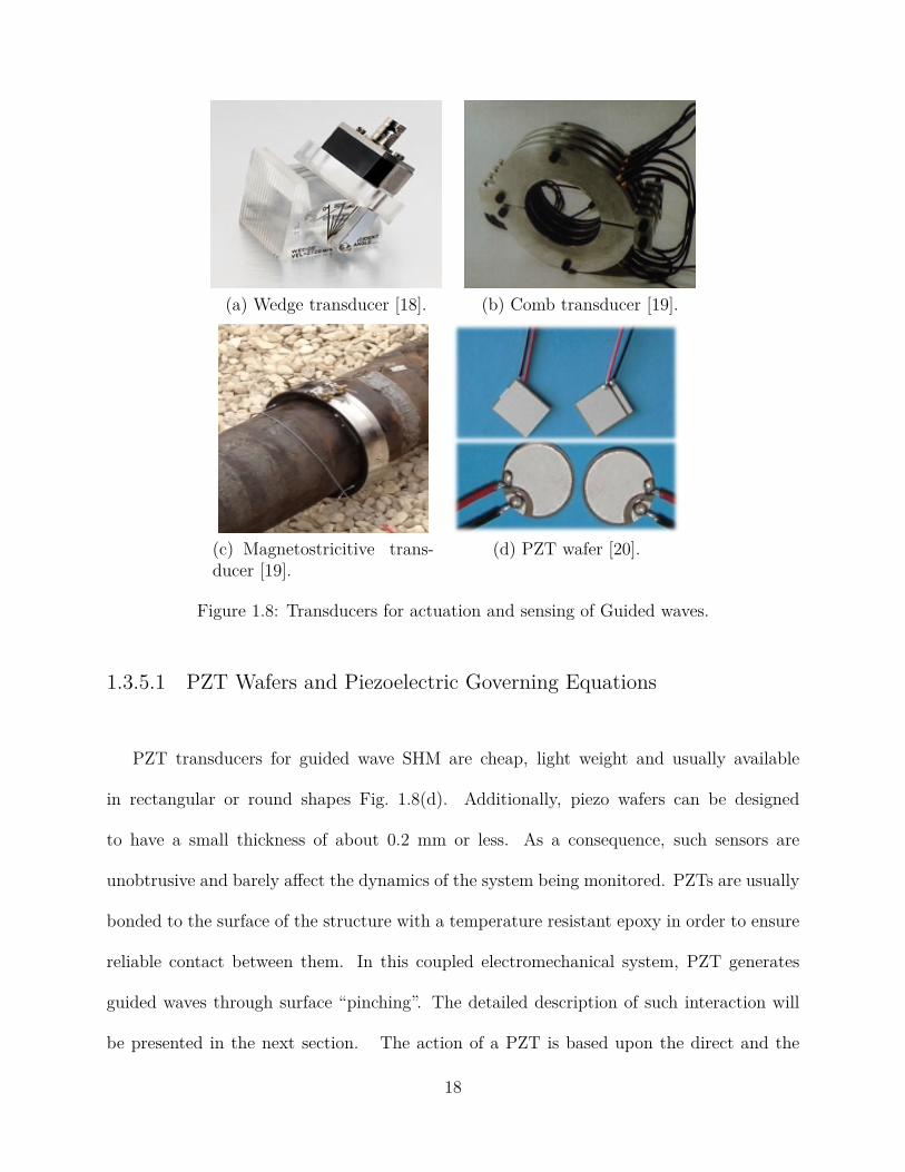
Eq. (1.33) corresponds to the equilibrium equation of the PZT, while Eq. (1.34) describes
the equilibrium of the structure. Note that the above equations are defined for symmetric
(σA;αA) and antisymmetric cases (σS ;αS) separately. In general, coefficient α needs to be
determined based on the actuation frequency and mode shapes. However, Giurgiutiu showed
that under the simplifying assumptions of uniform stress distribution for symmetric case and
linear stress distribution for the antisymmetric case, the coefficient α takes on the values of
1 and 3. Further, the shear lag solution can be evaluated as the superposition of symmetric
and antisymmetric excitations: σ = σA+σS and α= αA+αS = 4. Taking this into account,
Eq. (1.33) and Eq. (1.34) can be further expressed in terms of strains to give the following
system
∂4εact∂x4 −Γ2∂2εact
∂x2 = 0 (1.35)
∂4εst∂x4 −Γ2∂2εst
∂x2 = 0 (1.36)
where Γ =√Gb(α+ψ)/Eatatbψ is a shear-lag constant and ψ = Et/Eata is a function of
geometry and material properties.
Finally, by solving Eq. (1.36) we obtain the expressions for induced surface stresses and
strains
τ(x) = taa
ψ
α+ψEaεv(ΓasinhΓx
coshΓa ) (1.37)
ε(x) = ψ
α+ψεv(1− coshΓx
coshΓa ) (1.38)
Eq. (1.35) defines new boundary conditions for Rayleigh-Lamb equations by applying
surface traction forces along the bonding layer. Therefore, energy transfer conditions for
symmetric and antisymmetric guided wave modes can be derived at this point.
24

Giurgiutiu [17] demonstrated that the total solution for displacement and strains across
Figure 1.13: Shear lag model: surface stress.
Figure 1.14: Shear lag model: surface strain.
the thickness of the interrogated structure can be obtained in the Fourier domain resulting
in the following relations
εx(x,t) = 12µ
∑ξS
τ(ξS)NS(ξS)DS ′(ξS)
ei(ξSx−ωt) + 1
2µ∑ξA
τ(ξA)NA(ξA)DA′(ξAS)
ei(ξAx−ωt)
ux(x,t) = 12µ
∑ξS
1ξS
τ(ξS)NS(ξS)DS ′(ξS)
ei(ξSx−ωt) + 1
2µ∑ξA
1ξA
τ(ξA)NA(ξA)DA′(ξAS)
ei(ξAx−ωt)
(1.39)
25

where the determinants DA; DS and the quantities NA; NA as well as DS ′ and DA′ are
defined as
NA = ξq(ξ2− q2)sinphsinqh (1.40)
DA = (ξ2− q2)2 sinphcosqh+ 4ξ2pq cosphsinqh (1.41)
DS ′=∂DS∂ξ
; DA′=∂DA∂ξ
(1.42)
where ξ – wavenumber, h – half plate thickness; p and q are defined in Eq. (1.15).
1.4.2 Ideal Bonding Assumption
It can be inferred from Fig. 1.13 that the stress and strain induced by the piezoelectric
transducer is largely concentrated near its edges. Hence, for the simplicity of analysis stress
can be approximated with reasonably good accuracy by two delta functions positioned at
the corresponding coordinates:
τ(x) = aτa[δ(x−a)− δ(x+a)] (1.43)
Considering the latter, the amplitude of individual frequency components transferred to
the structure through the ideal adhesive layer can be obtained by assuming the harmonic
excitation of the PZT:
τ(x) = aτ0[δ(x−a)− δ(x+a)]ejωt (1.44)
26

Upon substitution of Eq. (1.44) to Eq. (1.39) we obtain the solution for surface strain and
displacement
εx(x,t) =−aτ0µ
[∑ξS
sinξSaτ(ξS)NS(ξS)DS ′(ξS)
ei(ξSx−ωt) +
∑ξA
sinξAaτ(ξA)NA(ξA)DA′(ξAS)
ei(ξAx−ωt)]
ux(x,t) =−aτ0µ
[∑ξS
sinξSaξSa
τ(ξS)NS(ξS)DS ′(ξS)
ei(ξSx−ωt) +
∑ξA
sinξAaξAa
τ(ξA)NA(ξA)DA′(ξAS)
ei(ξAx−ωt)]
(1.45)
The displacement across the thickness of the structure uy as well as the stresses τyx and τyy
can be found upon substitution of the same constants obtained from the boundary conditions
in the corresponding equations (see Appendix A).
Figure 1.15: Actuation using surface-bonded PZT.
Fig. 1.15 illustrates the surface strain induced by the PZT along the x-direction for the
fundamental S0 and A0 modes that exist at all frequencies. The relations are evaluated for
the case of 2-mm thick aluminum plate with 7-mm square PZT ideally bonded to its surface.
Interestingly, at some frequencies such as 390 kHz the two modes are actuated with high
amplitudes. However, some frequencies reject both modes (e.g. 710 kHz). This fact makes
27

it possible to use so called mode tuning in order to amplify some modes with respect to the
others and achieve mode tuning.
1.4.3 Voltage Output of the PZT Sensor
Earlier in this section the transduction of guided waves to the structure was analyzed.
However, in experiments one usually measures voltage output of the PZT sensor. Therefore,
we need to consider the parameters on which the voltage depends. Piezo-sensor response to
vibration was derived by Ragavan and Cesnik [25]. Voltage between the electrodes of the
PZT is proportional to the superposition of strains across the area of its bottom face
V = Q
C= Y 11hcg31Sc(1−ν)
∫SεiidS (1.46)
where Q – electric charge accumulated by the piezoelement; C – capacitance of the PZT;
Sc – surface area of the PZT; hc − thickness of the piezo; g31 − corresponding entry from
the matrix of piezoelectric constants; Y 11 − the in-plane Young’s modulus of the sensor and
ν − the Poisson’s ratio; εii – the sum of in-plane surface strains.
In the case of rectangular actuator Eq. (1.46) takes the form
V = Y 11hcg314s1s2(1−ν)
∫ xc+s1xc−s1
∫ yc+s2yc−s2
[∂u1∂x1
+ ∂u2∂x2
]dx1dx2 (1.47)
where s1 and s2 are half-length and half-width of rectangular PZT; xc and yc are coordinates
of the geometric center of the PZT. Clearly, V is linear with respect to the summation of
the in-plane surface strains.
28

CHAPTER 2
Signal Analysis in Guided Wave SHM
2.1 Overall Approach to Damage Detection
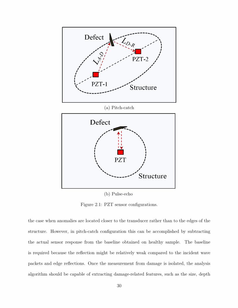
Guided wave SHM with distributed PZT sensor networks employs pitch-catch and pulse-
echo damage detection methods (Fig. 2.1). In pitch-catch mode, one piezoelement actuates
guided waves in order to interrogate the structure and the collocated element measures the
response. If the wavelength of the GW mode is comparable to the size of the defect, the
incident wave will be reflected and captured by the receiving PZT. Compared to pitch-
catch, pulse-echo utilizes the same transducer to perform excitation and sensing. This is
accomplished by electronic switching between the corresponding circuits of the hardware
node.
Once the signals from all sensor pairs in the network are recorded, one needs to isolate
Lamb wave scattering from anomalies in contrast to reflections from various boundaries in
the complex structure. For pulse-echo mode damage reflections could be easily identified in
29
(a) Pitch-catch
(b) Pulse-echo
Figure 2.1: PZT sensor configurations.
the case when anomalies are located closer to the transducer rather than to the edges of the
structure. However, in pitch-catch configuration this can be accomplished by subtracting
the actual sensor response from the baseline obtained on healthy sample. The baseline
is required because the reflection might be relatively weak compared to the incident wave
packets and edge reflections. Once the measurement from damage is isolated, the analysis
algorithm should be capable of extracting damage-related features, such as the size, depth
30

and location of the defect. For this purpose, Probability Diagnostic Imaging (PDI) has been
widely adopted in recent works on guided wave SHM.
2.2 Probability Diagnostic Imaging
Essentially, PDI estimates the most probable location of defect from the TOF of individ-
ual reflection [26]. The method may combine pulse-echo and pitch-catch configurations of
sensors in an active network to acquire signal features associated with damage. Assuming the
GW signal contains a single mode, damage location could be easily identified by measuring
the Time-of-Flight of a wave packet reflected by the anomaly. This ToF includes the time
required for the wave packet to travel from the actuator to the defect and the time to reach
from defect to the receiver. Hence, the ToF corresponding to the reflection from damage can
be computed using the equation
ToF =LA−D+LD−R
cgr(2.1)
It follows that damage must be located on the locus of an ellipse defined by each actuator-
receiver pair. Since measurement errors are always present, PDI assigns the 2D Gaussian
probability density function to each pixel on every ellipse of the array
F (zi) =∫ zi
−∞f(zi)dz (2.2)
I(xm,yn) = 1− [F (zi)−F (−zi)] (2.3)
31
where I(xm,yn) − illumination function, (xm,yn) − coordinates of the specific point on
the grid, F (zi) − Gaussian cumulative probability function, f(zi) − Gaussian probability
density function.
As a result, the regions of the image where more of the ellipses overlap are illuminated
with higher intensity, indicating the most probable location of the damage.
2.3 Challenges in Signal Processing of Guided Waves
Damage detection algorithms employed in SHM systems with active PZT sensor networks
assume unimodal propagation of guided waves. For instance, PDI requires the knowledge
of group velocity for accurate damage detection, that follows from Eq. (2.1). Actuation
of a single GW mode can be accomplished with the help of collocated PZT pair or fre-
quency tuning as discussed in previous sections. However, the use of collocated actuators is
somewhat impractical for SHM, since it doubles the number of transducers in the network.
Moreover, both surfaces of the structure may not be always accessible. On the other hand,
mode tuning requires only one piezoelement for selective mode excitation. Nevertheless,
this approach does not guarantee the complete rejection of other modes with respect to the
dominant mode. This follows from the fact that in practice the bonding layer between the
PZT and structure is not ideal as compared to theoretical assumptions made in derivation of
Eq. (1.39). In addition, one needs to consider mode shapes which would maximize the sensi-
tivity of the system to specific types of defects, but in general the optimal mode shape may
correspond to frequencies at which the sweet spot does not exist. In the case when actuation
is not strictly mode selective, multiple modes will propagate in the structure with different
32
amplitudes and velocities, interfering with each other as well as with reflections from edges
and structural defects. Given the monolitic PZT elements are equally sensitive to u1 and u2
displacements (Eq. (1.47)), the collected signals will contain reflections from all directions of
wave propagation across the surface of the structure. In terms of damage detection, all of the
above makes the interpretation of GW signals a fairly complicated problem. It is apparent
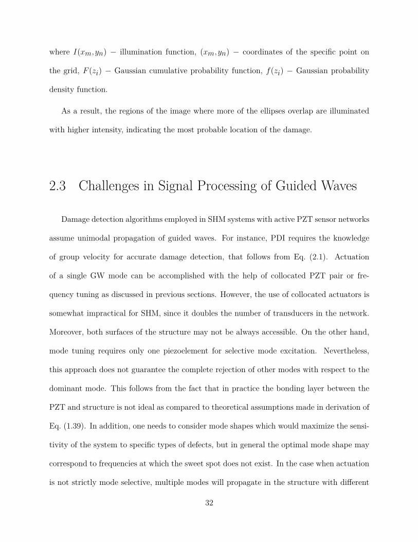
Figure 2.2: Approach to signal processing.
that GW signals should be subjected to some pre-processing stage or Mode Decomposition
(MD) in order to decouple the contributions from different modes and facilitate the correct
performance of diagnostic imaging. Hence, the overall approach to signal processing in SHM
systems with distributed PZT sensor networks can be now illustrated by the Fig. 2.2.
As will be seen next, development of MD algorithms requires the selection of features
to classify the modes and forward model to simulate wave propagation in the structure.
Moreover, the MD algorithm should process signals automatically and it should be fast
enough to be used in real-time monitoring systems. This study focuses on the development of
decomposition algorithms which could be established with the help of time-frequency analysis
and iterative methods such as matching pursuits. In the next section, a brief overview of
the above methods will be presented.
33

2.4 Characteristic Features for Mode Identification
The narrowband actuation of guided waves (e.g. Morlet wavelet, Fig. 2.3(a)) on any
non-flat region of dispersion curves introduces a difference between the velocities of lower
and higher frequency components of the generated wave packets. Consider the group delay
of a single wave packet [38]:
τg(ω) = ∂ϕ(ω)∂ω
= ∂k(ω)x0∂ω
= x0∂ω/∂k(ω) = x0
cgr(2.4)
where ϕ(ω) – phase of the actuation waveform, k(ω) – wavenumber, x0 – propagation dis-
tance.
(a) Morlet wavelet (b) Fourier transform of the Morletwavelet
Figure 2.3: Narrowband actuation waveform.
The group delay is in inverse relation with the group velocity, therefore it can be an
informative feature about modal content of a particular GW signal. For example, for a given
narrowband actuation frequency range of Morlet wavelet (Fig. 2.3(b)), the group delay slope
of S0 mode is positive and that of A0 is negative if GW propagates in a 2-mm thick aluminum
34

Figure 2.4: Dispersion curves of a 2-mm thick aluminum plate corresponding to the spectrumof the Morlet wavelet.
plate with dispersion curves shown in Fig. 2.4. It follows that information about the mode
can be extracted from the slopes of the instantaneous frequency components of the signal
on a time-frequency plane.
2.5 Time-Frequency Representations in GW SHM
Time-frequency representation (TFR) is an important aspect of signal processing in
Guided wave SHM, since it provides tools for mode identification. Moreover, TFRs can
be used in a combination with some post-processing such as ridge or skeleton extraction in
order to isolate wave packets and locate their time-frequency centers. Unlike well established
Fourier transform, which is suitable for analysis of stationary signals only, TFRs allow for
determining the instantaneous frequency components of the signal as a function of time. In
other words, the TFRs are capable of analyzing a given evolutionary time series in joint time
and frequency domain. TFRs can be broadly classified as atomic decompositions (linear
35
TFRs) and energy distributions (quadratic TFRs). It should be mentioned that both classes
have been employed in different applications involving GW signal analysis. A brief overview
of TFRs is given in the next section.
2.5.1 Linear Time-Frequency Representations
2.5.1.1 Short Time Fourier Transform
Linear TFRs also called atomic representations decompose original signal into a weighted
sum of elementary functions. One of the simplest and most intuitive examples of a linear TFR
is the Short Time Fourier Transform (STFT). The GW signal to be processed is multiplied
by a window function with a short time support. Then the Fourier Transform of the signal
within the window is taken as it moves along the time axis. This results in a two-dimensional
time-frequency representation
STFTx(t,ω) = 12π
∫ +∞−∞
s(τ)h(τ − t)e−jωtdτ (2.5)
where x(t) − original signal; ω − radian frequancy; τ − time lag variable.
Window function is always chosen to be shorter compared to the length of the signal
in order to provide localized information about its spectrum. Additionally, the window is
designed to suppress the original signal at the ends of the selected support in order to prevent
spectrum leakage [27]. However, the main drawback of STFT is a trade-off between time
and frequency resolution. Considering the signal which is perfectly localized in time
x(t) = δ(t− t0) (2.6)
36

the time resolution of STFT will be affected by the length of the analysis window
STFTx(t,ω) = h(t− t0)e−jωt0 (2.7)
Similar relation holds for frequency resolution indicating that long analysis windows yield
less frequency spreading. This result may also be interpreted from the perspective of time-
bandwidth product theorem. The time-bandwidth product theorem, or more generally, the
uncertainty principle is a fundamental concept of time-frequency analysis based upon the
properties of Fourier transform pairs. The uncertanity principle states that the joint time-
frequency resolution is always limited and the TFR cannot provide perfect localization in
time and frequency simultaneously. The above concept can be well illustrated by considering
the energy density of the signal |x(t)|2 and its Fourier transform |X(ω)|2 as probability
distributions [28]. Assuming the signal has finite energy
E =∫ +∞−∞
|x(t)|2 dt <+∞, (2.8)
one can calculate the average time tm at which the signal is centered and the average
frequency ωm of its spectrum
tm = 1E
∫ +∞−∞
t |x(t)|2 dt (2.9)
ωm = 1E
∫ +∞−∞
ω |X(ω)|2 dω (2.10)
37

Then the time and frequency spreading can be defined as variances
σ2t = 4π
E
∫ +∞−∞
(t− tm)2 |x(t)|2 dt (2.11)
σ2ω = 4π
E
∫ +∞−∞
(ω−ωm)2|S(ω)|dω (2.12)
where σt − time variation and σω − bandwidth. It follows that the energy of the signal is
concentrated in the area proportional to the time-bandwidth product σtσω, and moreover
σ2t σ
2ω ≥
14
(2.13)
Depending on selected window, STFT uniformly tiles time-frequency plane in rectangles
schematically shown in Fig. 2.5. Eq. (2.13) holds for signals pre-multiplied by Gaussian
Figure 2.5: Time-frequency tiling of STFT.
windows and therefore, it also determines the time-frequency resolution of STFT. It should be
38

noted that STFT was employed in some works on guided wave signal processing [29], but in
general, it does not provide the best capability to resolve overlapped multimodal reflections.
Hence, methods for reducing the spread of STFT is discussed later in this section.
2.5.1.2 Continuous Wavelet Transform
In recent decades, Continuous and Discrete Wavelet Transforms have been widely adopted
in GW signal processing. In contrast to the STFT, which decomposes a given signal in
terms of sinusoids with infinite duration, wavelet transform projects the signal on a family
of oscillatory functions (wavelets) with limited time support
CWTx(a,b) = 1√|a|
∫ +∞−∞
x(t)ψ∗(t− ba
)dt (2.14)
Wavelet families can be easily constructed from an elementary function ψ(t) called mother
wavelet by dilations and translations using scaling factor a > 0 and time shift b. CWT
Figure 2.6: Time-frequency tiling using dyadic wavelets.
39

operates with continuous time, but time-scale parameters are often sampled on dyadic grid,
which allows for efficient implementation of the algorithm
CWTj,k = CWT{x(t);a= 2j , b= k2j} j,k ∈ Z (2.15)
Clearly, the resulting distribution expresses the signal with respect to translation and
scale rather than time and frequency. One of the characteristic features of CWT is the way
the time-frequey plane is tiled (Fig. 2.6). It can be noticed that the resolution of CWT
turns out to be scale dependent: lower frequency components of the analyzed signal can
be well resolved in scale but poorly in time; conversely, higher frequency components are
better localized in time, but the corresponding scale resolution is low. As a consequence,
CWT can be useful for multiresolution analysis of broadband GW signals. Additionally, its
discrete version (Discrete Wavelet Transform) is shown to be efficient in applications which
require denoising [30]. However, CWT is still subject to uncertanity principle and its joint
resolution in time and scale is also limited.
2.5.1.3 Chirplet Transform and Warping Operators
Chirplet Transform and TFRs employing warping operators are natural extension of
previously discussed atomic decompositions. Chirplet transform expands a signal in terms
of a basis of multi-scale wavelets with linear frequency modulation also called chirplets.
CTx =∫ +∞−∞
x(t)g∗t0,ω0,s,q,p(t)dt
gt0,ω0,s,q,p(t) = Tt0Fω0SsQqPph(t)(2.16)
40

where h(t) is window function, Tt0 − time shift of the chirplet, Fω0 − frequency shift, Ss
− scaling parameter, Qq − frequency shear and Pp − time shear parameters.
Figure 2.7: Warped tiling of time-frequency plane.
The additional degrees of freedom, namely shear parameters, control the chirp rate of
generated functions and enable rotation of elementary time-frequency cells. In fact this
property is useful when some prior information about localization of signal components on
a TF plane is known. Further, in recent works on GW signal processing warping operators
have been introduced. The detailed description of the concept can be found in [31]. TFRs
based on warping functions allow for tiling of time-frequency plane in a fashion that matches
the group velocity curves of different materials. Many works employing such TFRs were
focused on obtaining the dispersion properties of the structure using broadband excitation
of guided waves. However, this is not very practical for online monitoring applications that
require minimal signal spreading and narrowband actuation.
41

2.5.2 Quadratic TFRs
Quadratic representations provide valuable information about time and frequency local-
ization of the energy carried by the GW signal. Naturally, such TFRs can be understood as
a joint energy density function that satisfies
Ex =∫ +∞−∞
∫ +∞−∞
ρx(t,ω) dtdω (2.17)
Another important properties of quadratic TFRs include the marginals
∫ +∞−∞
ρx(t,ω) dt= |X(ω)|2
∫ +∞−∞
ρx(t,ω) dω = |x(t)|2(2.18)
It can be shown that these are satisfied by energy distributions and more generally, by
TFRs of Cohen′s class [32]. However, many GW signal processing applications for SHM of
metal and composite structures involve spectrograms and scaleograms defined as a squared
modulus of STFT and CWT correspondingly:
Sx(t,ω) = |STFT (t,ω)|2 (2.19)
Cx(t,ω) = |CWT (t,a)|2 (2.20)
The above representations are non-negative and always real-valued. However, they do not
satisfy conditions in Eq. (2.18) and therefore can be considered as transition groups [32] from
atomic decompositions to properly defined energy distributions. This can be explained by
the fact that spectrograms and scaleograms mix the energy of the window or wavelet function
42

with that of the original signal. Another interesting property of these representations is a
quadratic superposition principle, which means that the spectrogram or scaleogram of the
sum of two signals is not the sum of the two separate representations
x(t) = y(t) + z(t) (2.21)
Sx(t,ω) = Sy(t,ω) +Sz(t,ω) + 2Re{Sy(t,ω)S∗z (t,ω)} (2.22)
However, it is true that for the above distributions the interference terms appear only at
points where the frequency components of the signal cross on a TF plane [28, 32]. Hence,
this drawback is not very critical. Finally, the time-frequency resolution of spectrograms
and scaleograms is limited exactly as it happens in the case of STFT or CWT.
2.5.2.1 Wigner-Ville Distribution
The first and most important TFR which belongs to the class of energy distributions is
Wigner-Ville distribution (WVD)
Wx(t,ω) =∫ +∞−∞
x(t+ τ
2)x∗(t− τ2)e−jωτdτ (2.23)
where x(t) − original signal; τ − time lag variable.
Wigner-Ville provides perfect time and frequency resolution, however it suffers from issues
related to cross-terms. Unlike spectrograms and scleograms, interference terms of WVD are
non-zero regardless of the time-frequency distance between the signal terms. Moreover, WVD
can yield negative values, which makes it difficult to interpret the results of decomposition.
43

The influence of interference terms can be alleviated by using special smoothing kernels in the
ambiguity domain [32]. However, this approach reduces the resolution of the representation.
2.5.3 Time-Frequency Reassignment
The reassigned TFRs define a different group of representations that has recently gained
attention in GW signal analysis. The reassignment procedure substantially reduces the
blurriness of the TFR and improves its mode identification capabilities. Moreover, reas-
signment suppresses the contributions from cross-terms and makes the TFR amenable to
post-processing. In general, it is known that any distribution of Cohen’s class can be ex-
pressed in terms of a 2D-convolution of the WVD with some kernel function
Cx(t,ω;Π) =∫ +∞−∞
∫ +∞−∞
Π(t− s,ω− ξ) Wx(s,ξ) ds dξ (2.24)
where Π(t− s,ω− ξ) − kernel, corresponding to a specific TFR; Wx(s,ξ) − Wigner-Ville
distribution of the signal.
Considering the above equation, it is noticed that essentially this operation performs
weighted averaging of the WVD of the signal around (t,ω) point [28]. Moreover, (t,ω)
defines the geometrical center of the local TF region limited by s and ξ. However, it would
be more logical to assign the local average to the center of gravity of the region. This is the
idea underlying time-frequency reassignment: reassignment procedure moves a particular
value of the original TFR from point (t,ω) to local center of gravity of WVD centroid at
44

(t, ω). Consequently, the reassigned coordinates are given by
t(x; t,ω) =∫ +∞−∞
∫ +∞−∞ sΠ(t− s,ω− ξ) Wx(s,ω) ds dω∫ +∞
−∞∫ +∞−∞ Π(t− s,ω− ξ)Wx(s,ξ) ds dξ
(2.25)
ω(x; t,ω) =∫ +∞−∞
∫ +∞−∞ ξΠ(t− s,ω− ξ) Wx(s,ξ) ds dξ∫ +∞
−∞∫ +∞−∞ Π(t− s,ω− ξ)Wx(s,ξ) ds dξ
(2.26)
The resulting TFR takes the form
CRx(t′,ω′;Π) =∫ +∞−∞
∫ +∞−∞
Cx(t,ω;Π) δ(t′− t(x; t,ω))δ(ω′− ω(x; t,ω)) dt dω (2.27)
In the same manner, the reassignment procedure can be also applied to the time-scale
(a) Ideal Time-Frequency representation (b) WVD of the signal
Figure 2.8: Ideal TFR and Wigner-Ville distribution of the signal.
energy distributions. It is possible to illustrate the performance of reassignment method
on specific examples. Fig. 2.8(a) demonstrates the synthetic signal generated in the time-
frequency domain with the help of Matlab Time-Frequency Toolbox [28]. The designed signal
consists of a linear and a polynomial chirp autoterms, which in some way approximate real
world GW signals. In turn, Fig. 2.8(b) − Fig. 2.10(b) present the comparison of different
45

(a) STFT of the signal (b) Smoothed WVD of the signal
Figure 2.9: Comparison of smoothed WVD and STFT of the signal (window length = 413points).
(a) Reassigned Smoothed WVD of the sig-nal
(b) Reassigned spectrogram of the signal
Figure 2.10: Comparison of reassigned smoothed WVD and reassigned spectrogram of thesignal (window length = 413 points).
TFRs applied to the time domain version of Fig. 2.8(a). Analyzing the obtained represen-
tations, one may notice that the spectrogram and smoothed WVD have significant amount
of blurring, while reassigned smoothed WVD and reassigned spectrogram are more localized
than other TFRs and yield nearly same results. However, real-time SHM applications re-
quire the TFR to be computationally efficient and easy to implement. From this perspective,
reassigned spectrogram computed with the help of Nelson’s method [33] can be considered
46

the best candidate for GW mode identification. Besides, the reassigned spectrogram also
satisfies the time and frequency shifts covariance and it is perfectly localized on linear chirp
signals and impulses
x(t) = Aej(ω0t+αt2/2) (2.28)
ω = ω0 +αt (2.29)
x(t) = Aδ(t− t0) (2.30)
t= t0 (2.31)
Finally, the performance of the reassigned spectrogram can be further enhanced by us-
ing Chirp-Z transform instead of computing the FFT for each window. This approach is
discussed in the next section.
2.6 Reassigned Spectrogram with Chirp Transform Ker-nel
At this point we develop the TFR based on reassigned spectrogram, which will be used
for mode decomposition algorithm discussed in this work. First, it is possible to derive an
explicit expression for re-mapped time and radian frequency coordinates in Eq. (2.25) and
Eq. (2.26). STFT can be described in terms of the Gabor Transform:
x(t) =∫ +∞−∞
∫ +∞−∞
ε(t,ω) ·Ψ∗(t, τ,ω)dτ dω (2.32)
47

The coefficients of the transform are defined as
ε(t,ω) =∫ +∞−∞
x(t) ·Ψ∗(t, τ,ω)dt (2.33)
The window function of STFT is expressed in terms of
Ψ∗(t, τ,ω) = h(t− τ)e−jω(τ−t) (2.34)
The coefficients of the Gabor Transform have amplitude and phase modulation
ε(t,ω) =∫ +∞−∞
x(t)h(τ − t)ejω(τ−t)dt= ejωτ∫ +∞−∞
x(t)h(τ − t)e−jωtdt= A(τ,ω)ejΦ(τ,ω)
(2.35)
The original signal can be reconstructed as
x(t) =∫ +∞−∞
A(τ,ω)h(τ − t)ej[Φ(τ,ω)−ωτ+ωt] (2.36)
The reassignment method that identifies the local energy centers, can be also explained by
the phase stationarity principle. In the case of Lamb wave signals, Eq. (2.36) represents the
oscillatory integral over a function that fluctuates rapidly under a slowly varying envelope.
The significant contributions to Eq. (2.36) come from the vicinity of points where the phase
is stationary, that is, where it goes through zero [34], which yields
x(t) = ∂
∂ω[j(Φ(τ,ω)−ωτ +ωt)]
x(t) = ∂
∂τ[j(Φ(τ,ω)−ωτ +ωt)]
(2.37)
48
Hence, the re-mapped time and frequency coordinates of the spectrogram can be computed
ast(τ,ω) = τ − ∂Φ(τ,ω)
∂ω
ω(τ,ω) = ∂Φ(τ,ω)∂τ
(2.38)
where −∂Φ(τ,ω)/∂ω is a local group delay and ∂Φ(τ,ω)/∂τ is the instantaneous frequency.
In this work, the reassigned spectrogram was implemented using the method, proposed
by Nelson [33]. It should be noted that the algorithm takes advantage of mathematically
defined cross-spectral surfaces to compute the coordinates in Eq. (2.38). In addition, the
reassigned spectrogram gets more informative when the window step is small and the FFT
window length is large. Therefore, the redundancy of the representation can be reduced and
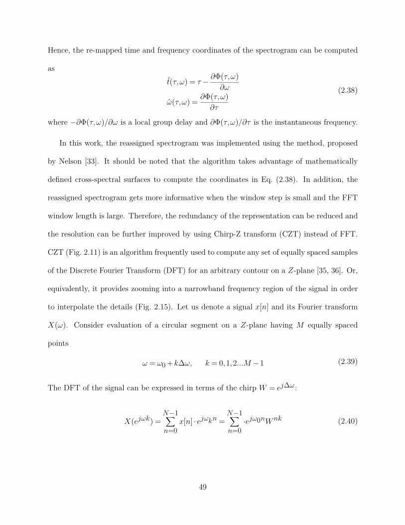
the resolution can be further improved by using Chirp-Z transform (CZT) instead of FFT.
CZT (Fig. 2.11) is an algorithm frequently used to compute any set of equally spaced samples
of the Discrete Fourier Transform (DFT) for an arbitrary contour on a Z-plane [35, 36]. Or,
equivalently, it provides zooming into a narrowband frequency region of the signal in order
to interpolate the details (Fig. 2.15). Let us denote a signal x[n] and its Fourier transform
X(ω). Consider evaluation of a circular segment on a Z-plane having M equally spaced
points
ω = ω0 +k∆ω, k = 0,1,2...M −1 (2.39)
The DFT of the signal can be expressed in terms of the chirp W = ej∆ω:
X(ejωk) =N−1∑n=0
x[n] · ejωkn =N−1∑n=0·ejω0nWnk (2.40)
49
Using the identity nk = 12 [n2 +k2− (k−n)2], we can derive the final expression for CZT
X(ejωk) =N−1∑n=0
x[n] · e−jω0nWn2/2Wk2/2W−(k−n)2/2 =Wk2/2(N−1∑n=0
g[n]W−(k−n)2/2)
(2.41)
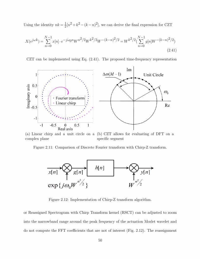
CZT can be implemented using Eq. (2.41). The proposed time-frequency representation
(a) Linear chirp and a unit circle on acomplex plane
(b) CZT allows for evaluating of DFT on aspecific segment
Figure 2.11: Comparison of Discrete Fourier transform with Chirp-Z transform.
Figure 2.12: Implementation of Chirp-Z transform algorithm.
or Reassigned Spectrogram with Chirp Transform kernel (RSCT) can be adjusted to zoom
into the narrowband range around the peak frequency of the actuation Morlet wavelet and
do not compute the FFT coefficients that are not of interest (Fig. 2.12). The reassignment
50

procedure developed in this section was applied to experimental data. Fig. 2.17 and Fig. 2.18
demonstrate the original STFT and RSCT of Lamb wave signal (Fig. 2.16) obtained on
2-mm thick aluminum plate (Fig. 2.13). Comparing the obtained results with STFT
Figure 2.13: Experimental set-up for obtaining GW signal: 600× 600× 2 mm aluminumplate.
Figure 2.14: FFT of GW signal.
Figure 2.15: CZT of GW signal. Zooming into 220-320 kHz range.
representation, it can be noticed that STFT is too blurred, but RSCT is capable of extracting
the information about the group delay (or slopes of the chirps corresponding to wave packets
of different modes). As expected from the previous section, the slope of S0 mode is positive
51

and that of A0 is negative. Interestingly, the amplitude-frequency centers presented in RSCT
are clearly different for S0 and A0 modes. This can be explained by frequency-dependent
strain transfer conditions from the PZT to the plate, discussed in Chapter 1.
Figure 2.16: Lamb wave signal (10240 samples).
Figure 2.17: STFT (window size 350 samples).
Figure 2.18: Reassigned spectrogram with CZT.
In general, Time-Frequency Representations allow for determining of GW modes with
well separated ToFs. However, the superposition of wave packets in time domain may result
52

in cancellation of some frequency components contained in the spectra of the original wave
packets. This creates some interference frequency transitions, that could be misinterpreted
as modes. Therefore, in this work we propose to complement time-frequency analysis with
Matching Pursuit method for mode decomposition.
2.7 Matching Pursuit (MP) algorithms in Guided wavesignal processing
Matching pursuit is an iterative algorithm which decomposes the signal into a linear
combination of functions (atoms) from an overcomplete frame D, called a dictionary [37]:
x=N−1∑n=0
αngγn (2.42)
where x – input GW signal, αn – weight coefficients corresponding to selected atoms from
the dictionary, gγn – frame functions, N – number of dictionary elements required for sparse
decomposition.
Given a dictionary with unit norm atoms, let Rn be the residual at nth approximation of
a signal x. MP projects the signal onto the elements of D in order to find the element that
has the highest correlation with it. In a classical formulation by Mallat and Zhang [37], this
iterative scheme consists of the following steps:
1. Specify initial conditions Rx= x0.
2. Find the atom with the highest inner product gγn = argmax〈Rn−1,gγn〉.
3. Subtract chosen atom from the signal and update the residual: Rn =Rn−1−〈Rn,gγn〉.
53

4. Stop the algorithm when the residue energy is sufficiently small or the maximum num-
ber of iterations nmax is exceeded.
Essentially, the redundancy of the dictionary allows MP to find the best projections onto
D thus making the original signal sparse in a coefficient domain. This property makes it
useful for solving complex minimization problems in Compressed Sensing and many other
applications. However, one of the key properties of MP that makes it useful for GW SHM, is
its ability to decompose the overlapped ultrasonic wave packets with the help of a properly
designed dictionary. In addition MP is robust to noise, which follows from the fact that
the dictionary contains only predefined noise-free functions. MP always aims at finding the
sparsest decomposition of the signal (e.g. linear combination requiring the least number of
frame-functions). For a properly constructed tight frame, the solution would be sparser if
more atoms are used. However, this increases the complexity of the problem and in general,
it is non-polynomial hard. Therefore, the choice of dictionary plays an essential role in MP
decomposition.
2.7.1 Gabor, Chirplet and Dispersion-based Dictionaries for MP
In GW analysis, elements of D are chosen to have shapes similar to those of ultrasonic
wave packets. Since Gabor and chirplet functions are very similar to oscillatory waveforms
with short time support, the matching pursuit algorithm with these dictionaries has been
explored by a number of researchers [38, 39, 40]. A unit energy chirplet can be expressed as
g(s,u,ω,c) = 1√sg(t−u
s) · ej[ω(t−u)+ c
2(t−u)2+ϕ] (2.43)
54
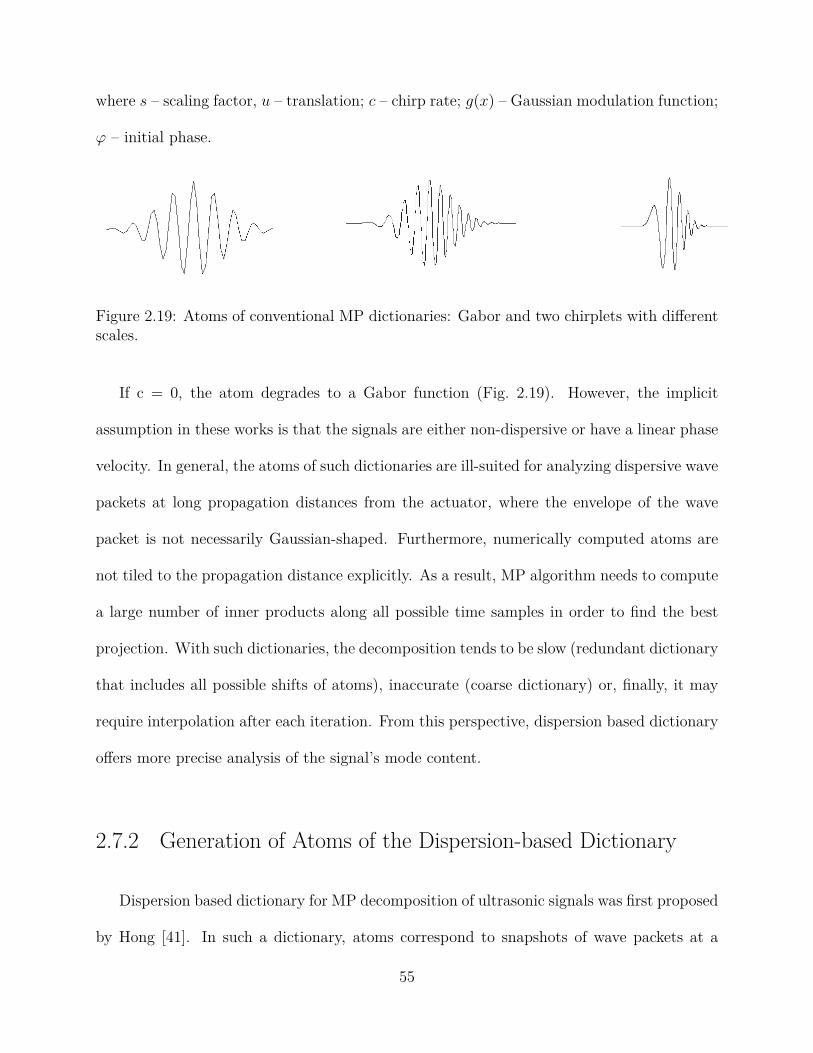
where s – scaling factor, u – translation; c – chirp rate; g(x) – Gaussian modulation function;
ϕ – initial phase.
Figure 2.19: Atoms of conventional MP dictionaries: Gabor and two chirplets with differentscales.
If c = 0, the atom degrades to a Gabor function (Fig. 2.19). However, the implicit
assumption in these works is that the signals are either non-dispersive or have a linear phase
velocity. In general, the atoms of such dictionaries are ill-suited for analyzing dispersive wave
packets at long propagation distances from the actuator, where the envelope of the wave
packet is not necessarily Gaussian-shaped. Furthermore, numerically computed atoms are
not tiled to the propagation distance explicitly. As a result, MP algorithm needs to compute
a large number of inner products along all possible time samples in order to find the best
projection. With such dictionaries, the decomposition tends to be slow (redundant dictionary
that includes all possible shifts of atoms), inaccurate (coarse dictionary) or, finally, it may
require interpolation after each iteration. From this perspective, dispersion based dictionary
offers more precise analysis of the signal’s mode content.
2.7.2 Generation of Atoms of the Dispersion-based Dictionary
Dispersion based dictionary for MP decomposition of ultrasonic signals was first proposed
by Hong [41]. In such a dictionary, atoms correspond to snapshots of wave packets at a
55
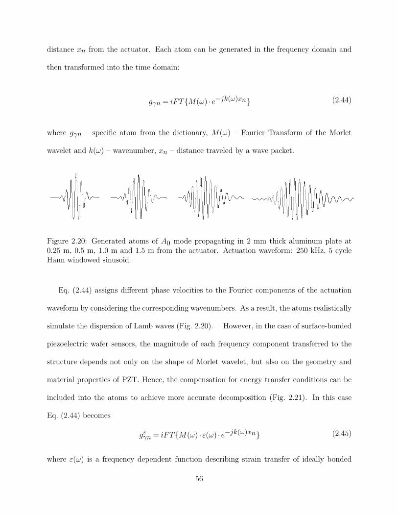
distance xn from the actuator. Each atom can be generated in the frequency domain and
then transformed into the time domain:
gγn = iFT{M(ω) · e−jk(ω)xn} (2.44)
where gγn – specific atom from the dictionary, M(ω) – Fourier Transform of the Morlet
wavelet and k(ω) – wavenumber, xn – distance traveled by a wave packet.
Figure 2.20: Generated atoms of A0 mode propagating in 2 mm thick aluminum plate at0.25 m, 0.5 m, 1.0 m and 1.5 m from the actuator. Actuation waveform: 250 kHz, 5 cycleHann windowed sinusoid.
Eq. (2.44) assigns different phase velocities to the Fourier components of the actuation
waveform by considering the corresponding wavenumbers. As a result, the atoms realistically
simulate the dispersion of Lamb waves (Fig. 2.20). However, in the case of surface-bonded
piezoelectric wafer sensors, the magnitude of each frequency component transferred to the
structure depends not only on the shape of Morlet wavelet, but also on the geometry and
material properties of PZT. Hence, the compensation for energy transfer conditions can be
included into the atoms to achieve more accurate decomposition (Fig. 2.21). In this case
Eq. (2.44) becomes
gεγn = iFT{M(ω) · ε(ω) · e−jk(ω)xn} (2.45)
where ε(ω) is a frequency dependent function describing strain transfer of ideally bonded
56
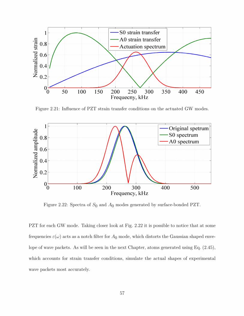
Figure 2.21: Influence of PZT strain transfer conditions on the actuated GW modes.
Figure 2.22: Spectra of S0 and A0 modes generated by surface-bonded PZT.
PZT for each GW mode. Taking closer look at Fig. 2.22 it is possible to notice that at some
frequencies ε(ω) acts as a notch filter for A0 mode, which distorts the Gaussian shaped enve-
lope of wave packets. As will be seen in the next Chapter, atoms generated using Eq. (2.45),
which accounts for strain transfer conditions, simulate the actual shapes of experimental
wave packets most accurately.
57
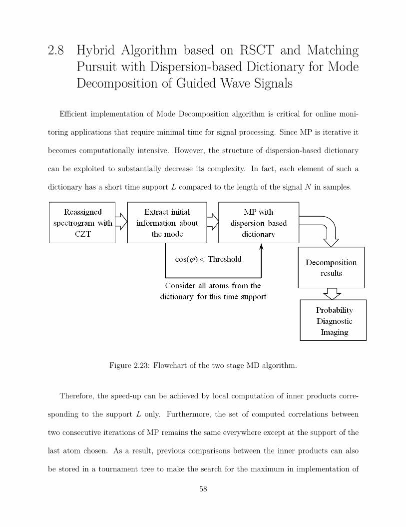
2.8 Hybrid Algorithm based on RSCT and MatchingPursuit with Dispersion-based Dictionary for ModeDecomposition of Guided Wave Signals
Efficient implementation of Mode Decomposition algorithm is critical for online moni-
toring applications that require minimal time for signal processing. Since MP is iterative it
becomes computationally intensive. However, the structure of dispersion-based dictionary
can be exploited to substantially decrease its complexity. In fact, each element of such a
dictionary has a short time support L compared to the length of the signal N in samples.
Figure 2.23: Flowchart of the two stage MD algorithm.
Therefore, the speed-up can be achieved by local computation of inner products corre-
sponding to the support L only. Furthermore, the set of computed correlations between
two consecutive iterations of MP remains the same everywhere except at the support of the
last atom chosen. As a result, previous comparisons between the inner products can also
be stored in a tournament tree to make the search for the maximum in implementation of
58
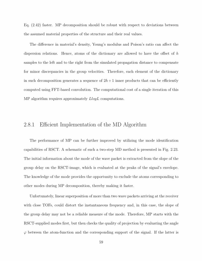
Eq. (2.42) faster. MP decomposition should be robust with respect to deviations between
the assumed material properties of the structure and their real values.
The difference in material’s density, Young’s modulus and Poison’s ratio can affect the
dispersion relations. Hence, atoms of the dictionary are allowed to have the offset of h
samples to the left and to the right from the simulated propagation distance to compensate
for minor discrepancies in the group velocities. Therefore, each element of the dictionary
in such decomposition generates a sequence of 2h+ 1 inner products that can be efficiently
computed using FFT-based convolution. The computational cost of a single iteration of this
MP algorithm requires approximately LlogL computations.
2.8.1 Efficient Implementation of the MD Algorithm
The performance of MP can be further improved by utilizing the mode identification
capabilities of RSCT. A schematic of such a two-step MD method is presented in Fig. 2.23.
The initial information about the mode of the wave packet is extracted from the slope of the
group delay on the RSCT-image, which is evaluated at the peaks of the signal’s envelope.
The knowledge of the mode provides the opportunity to exclude the atoms corresponding to
other modes during MP decomposition, thereby making it faster.
Unfortunately, linear superposition of more than two wave packets arriving at the receiver
with close TOFs, could distort the instantaneous frequency and, in this case, the slope of
the group delay may not be a reliable measure of the mode. Therefore, MP starts with the
RSCT-supplied modes first, but then checks the quality of projection by evaluating the angle
ϕ between the atom-function and the corresponding support of the signal. If the latter is
59

small enough, the RSCT-proposed projection is subtracted from the residual, otherwise, all
possible atoms are considered.
60

CHAPTER 3
Experimental Studies
3.1 Defect Localization in Metal Structures
Performance of the proposed MD method was tested on 2-mm thick 6061-aluminum al-
loy plate with a notch (Fig. 3.10(a)). Lamb waves were generated with a pair of collocated
7×8×0.2 mm transducers PZT1-1, PZT1-2 and were sensed by the receiver PZT-2. Morlet
wavelet excitation (10V) at 250 kHz center frequency was applied to PZT-1 using the arbi-
trary waveform generator 33220A (Agilent, Inc.) in order to activate S0 and A0 modes in
the plate. Data were sampled from the output of the charge amplifier with the help of the
digital oscilloscope DSO1004 (Agilent, Inc.).
For a given plate thickness, both S0 and A0 modes have high energy, therefore neither
of them can be ignored in the analysis. In the set-up in Fig. 3.1(b), S0 mode gets reflected
from the defect before A0 reaches the receiver, hence their wave packets arrive with close
TOFs. In order to test the MD, Lamb waves are first actuated with a single surface bonded
61
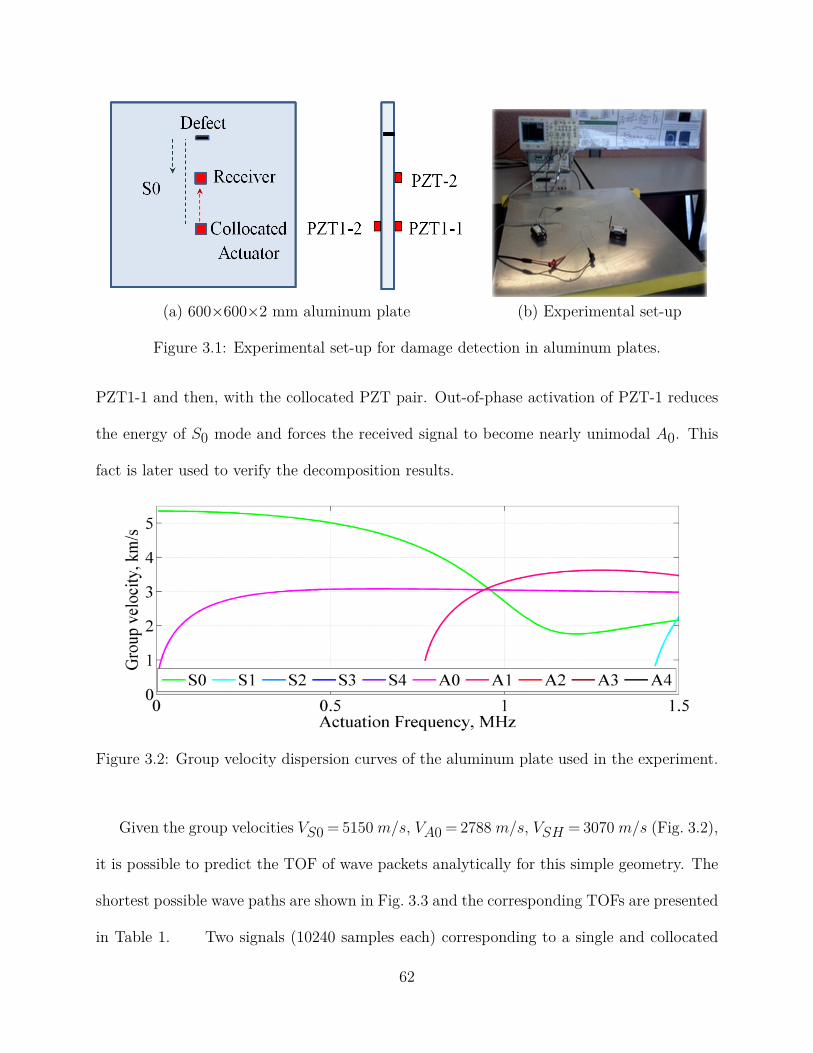
(a) 600×600×2 mm aluminum plate (b) Experimental set-up
Figure 3.1: Experimental set-up for damage detection in aluminum plates.
PZT1-1 and then, with the collocated PZT pair. Out-of-phase activation of PZT-1 reduces
the energy of S0 mode and forces the received signal to become nearly unimodal A0. This
fact is later used to verify the decomposition results.
Figure 3.2: Group velocity dispersion curves of the aluminum plate used in the experiment.
Given the group velocities VS0 = 5150 m/s, VA0 = 2788 m/s, VSH = 3070 m/s (Fig. 3.2),
it is possible to predict the TOF of wave packets analytically for this simple geometry. The
shortest possible wave paths are shown in Fig. 3.3 and the corresponding TOFs are presented
in Table 1. Two signals (10240 samples each) corresponding to a single and collocated
62

Figure 3.3: Possible wave paths from the actuator to the receiving PZT.
Figure 3.4: GW actuation using single surface-bonded PZT-1.
Figure 3.5: Reassigned spectrogram with CZT.
Figure 3.6: Collocated actuation of Guided waves.
63
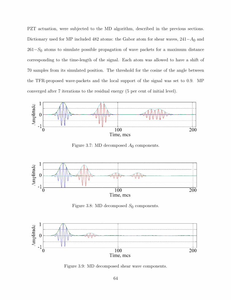
PZT actuation, were subjected to the MD algorithm, described in the previous sections.
Dictionary used for MP included 482 atoms: the Gabor atom for shear waves, 241−A0 and
261−S0 atoms to simulate possible propagation of wave packets for a maximum distance
corresponding to the time-length of the signal. Each atom was allowed to have a shift of
70 samples from its simulated position. The threshold for the cosine of the angle between
the TFR-proposed wave-packets and the local support of the signal was set to 0.9. MP
converged after 7 iterations to the residual energy (5 per cent of initial level).
Figure 3.7: MD decomposed A0 components.
Figure 3.8: MD decomposed S0 components.
Figure 3.9: MD decomposed shear wave components.
64

Wave path Length, cm Time-of-Flight S0, µs Time-of-Flight A0, µs1 14.5 28.4 52.02 (defect) 36.5 71.5 130.53 53.1 104.1 –4 62.0 121.4 –5 62.0 130.2 –
Table 3.1: Length of possible wave paths and corresponding Times-of-Flight for S0 and A0modes.
Number of wave path 1 2 3 4 5SO Analytical / MD ToF, µs 28.4/30.2 71.5/69.5 104.1/102.1 121.4/– 130.2/–SO Experim. / MD Dist., cm 14.5/15.5 36.5/37.2 53.1/52.6 62.0/– 66.5/–AO Analytical / MD ToF, µs 52.0/50.5 130.9/132 – – –AO Experim.l / MD Dist., cm 14.5/15.2 36.5/35.9 – – –
Table 3.2: Comparison of analytic and MD-extracted Times-of-Flight for S0 and A0 modes.
Separated modal components of the signal obtained with a single PZT actuation (Fig. 3.4)
are presented in Fig. 3.7−Fig. 3.9. Comparing the results with analytical calculations (Ta-
ble 3.1), it is possible to notice that MD has correctly extracted the TOF of S0 and A0 defect
reflections and, at the same time, identified the incident S0, A0 and shear mode wave pack-
ets. The signal reconstructed as a superposition of A0-selected atoms, correlates well with
the experimental waveform obtained with the collocated PZT set-up (Fig. 3.7 and Fig. 3.6).
Hence, the MD algorithm can be utilized to provide diagnostic imaging in the case when
more than one high-energy mode is present in the structure. In particular, such an approach
can be implemented without a baseline if the defect is large enough to be considered a strong
reflector. Otherwise, the algorithm should be applied to the differenced signal.
The MD-based PDI was tested on the similar 60×60 cm and 2-mm thick aluminum plate,
but with a different positioning of sensors shown in Fig. 3.10(a). The method used Lamb wave
65

(a) 600×600×2 mm alu-minum plate
(b) PDI-generated ellipses (c) Most probable damage lo-cation identified with the helpof PDI
Figure 3.10: Damage detection in 2-mm thick aluminum plate.
Figure 3.11: Signal from PZT 1-2 sensor pair.
Figure 3.12: Signal from PZT 2-3 sensor pair.
data recorded for each pair of sensors in pitch-catch configuration. Reflections of S0 mode
were chosen to identify the defect location. Typical sampled signals are presented in Fig. 3.11
and Fig. 3.12. It should be noted that S0 reflection from damage had minimal overlap with
other wave packets in the signal obtained from sensor pair PZT1-PZT2. However, for a sensor
66
pair PZT1-PZT3, it merged with A0 incident wave packet. In this case, the capabilities
of MD algorithm were fully exploited to extract information about the overlapped modes
and their ToFs. The S0 mode components resulting from MD were utilized as an input
for a standard PDI algorithm. Ellipses computed for each sensor pair were merged and
thresholded to obtain the most probable damage location. The coordinates identified for the
damage location was within a deviation of less than 1 cm from its true geometric coordinates
of the machined defect (Fig. 3.10(c)).
3.2 Defect Localization in Woven Composite Structures
Over the last decade, composite materials have become widely used in aerospace, civil,
automotive and other industries. A rapid development of composites for various applica-
tions can be explained by their advantages such as high strength, fracture toughness and
light weight. Composite laminates are manufactured from multiple components such as fiber
and matrix. However, the main challenge in engineering problems involving such materials
is anisotropy: mechanical properties differ with respect to the direction considered for anal-
ysis. Moreover, composites usually undergo complicated deformations when a tensile force is
applied in a particular direction. For instance, stretching of composite plate can cause shear
deformations, bending and even twisting. In a Classical Laminate Theory (CLT), mechanical
behavior of a single-layered laminate can be described by the contracted system of elasticity
equations
67

σ1
σ2
σ3
σ4
σ5
σ6
=
C11 C12 C13 C14 C15 C16
C22 C23 C24 C25 C26
C33 C34 C35 C36
C44 C55 C56
sym C55 C56
C66
ε1
ε2
ε3
γ4
γ5
γ6
(3.1)
The coefficients of Eq. (3.1) are grouped into the stiffness matrix [C], whose entries relate
stresses σij applied to the structure with the corresponding strains εi (note that γi = 2εi for
i = 4,5,6). The entries of the stiffness matrix Cij uniquely define material properties in all
possible directions. Additionally, the stiffness matrix is symmetric and contains 36 elements,
at most 21 of which can be independent. It should be noted that knowledge of stiffness
matrix is required for accurate GW signal processing, because it allows one to calculate the
phase and group velocity dispersion curves of a composite material used in experimental
studies. The latter can be accomplished using a theory of Guided wave propagation in
general anisotropic media and Transfer Matrix Method developed by Nayfeh [42]. Woven
composites used in this work were manufactured with layers having woven fibers oriented
in two principle directions x1 and x2. Such design significantly reduces the anisotropy of
mechanical properties in the corresponding plane. However, in this case CLT provides only
an approximate representation of the stiffness matrix. Nevertheless, the Young’s moduli and
Poisson’s ratios were determined from tensile tests: E11 = 30 GPa, E22 = 30 GPa, G12 = 10
GPa, ν12 = 0.4 (ν13 and ν23 were assumed to be equal to ν12, as well as G12 = G13 = G23)
and later the stiffness matrix was assumed to have the form of an orthotropic material.The
68

Figure 3.13: Phase velocity dispersion curves generated for 5-mm thick 8-layer compositeplate with the help of Transfer Matrix method.
expressions of Cij entries of the above matrix in terms of Young’s moduli and Poisson’s
ratios are presented in Appendix B.
C11 C12 C13 0 0 0
C12 C22 C23 0 0 0
C13 C23 C33 0 0 0
0 0 0 C44 0 0
0 0 0 0 C55 0
0 0 0 0 0 C66
(3.2)
The dispersion relations were obtained with the help of Transfer Matrix method assuming
a single 5-mm thick layer of composite material, since it was woven and cured (Fig. 3.13). In
general, dispersion curves can be also determined experimentally with the help of broadband
laser actuation [43] and processing of collected signals with specially designed TFRs as
discussed in Chapter 2. Alternatively, the elastic constants can be estimated using Genetic
69

Algorithm based inversion of ToF data obtained from multiple sensors and different directions
of GW propagation [44].
(a) Laser vibrometer set-up for measuringthe ToF of A0 mode wave packets
(b) Woven composite plate and pointsfor taking laser vibrometer measure-ments
Figure 3.14: Damage detection in 2-mm thick aluminum plate.
In the case of composite materials we additionally need to determine the variation of
the group velocity with respect to the propagation angle to ensure that the performance of
PDI after Mode Decomposition is still accurate. For this purpose, a laser vibrometer can be
utilized to measure the ToF of wave packets that propagate in different directions from the
actuating PZT (Fig. 3.14(b)). The vibrometer involved in this work was capable of sensing
displacements along the direction of the laser beam only, hence vertical orientation of the
head provided measurements of out-of-plane displacements corresponding to antisymmetric
modes. Guided waves were actuated in 5-mm thick composite plate with a 7×8×0.2 mm
PZT wafer using Morlet wavelet centered at 75 kHz. Fig. 3.15 illustrates the extracted
group velocities of the A0 mode from the collected GW signals. Difference of A0 mode
group velocity at various propagation angels is less than 8 % at frequencies less than 200
70

Figure 3.15: Variation of the group velocity of A0 mode actuated at 70 kHz with respect tothe direction of propagation in a 5-mm thick 8-layer woven composite plate.
kHz. It follows that the Probability Diagnostic Imaging can be still applied to locate damage
in woven composite materials without major modification. Therefore, it is possible to use
the approach for damage detection described in the previous section. However, composite
samples introduce more intensive scattering of Guided waves than aluminum plates and
therefore, baseline subtraction is needed to identify reflection from damage.
The experimental set-up for identifying defects in composite samples is presented in
Fig. 3.17(a). 60×45×5 mm woven composite plate with six surface mounted PZT wafers
was subjected to impact damage Fig. 3.17(b). Using the same procedure as in the previous
section, Guided waves were actuated at 75 kHz and pitch-catch approach was employed to
collect baselines and signals containing damage signatures from all sensor pairs. The example
71

(a) Composite plate with impact damage (b) Impact damage
Figure 3.16: Composite samples used in experimental studies.
(a) PDI generated ellipses on compositesample
(b) Most probable damage location
Figure 3.17: Probability Diagnostic Imaging on composite samples.
Figure 3.18: Baseline and differenced signal obtained by PZT-6 and PZT-2 sensor pair oncomposite plate.
of differenced signal is demonstrated in Fig. 3.18. It can be noticed that only A0 mode is
sensitive to surface defects. Thus, the signal contains a single A0 wave packet reflecting from
72
damage, which can be also identified by MD algorithm. However, in this case the problem
simplifies and the ToF of A0 mode can be extracted directly from the peak of its envelope.
Analyzing signals from multiple sensor paths, Probability Diagnostic Imaging is applied to
construct ellipses corresponding to the most probable damage location Fig. 3.17(a). Finally,
similar to the case of aluminum plates, damage site can be correctly identified by thresholding
on the image Fig. 3.17(b) or computing its geometric mean.
73
CHAPTER 4
Conclusions and Future Work
This work presented a new approach for processing of multi-modal Lamb wave signals,
which is a critical requirement for accurate identification of damage sites with the help of
distributed PZT sensor networks. Two-stage Mode Decomposition algorithm, employing the
Reassigned Spectrogram with Chirp Transform kernel and Matching Pursuit with dispersion-
based dictionary, was proposed to identify and separate high energy S0 and A0 modes
propagating in aluminum and woven composite plates. The MP dictionary was designed to
account for strain transfer conditions between the PZT and the structure, which provided a
good agreement between the generated dictionary atoms and experimentally obtained wave
packets. It was demonstrated that MD-extracted information about the mode, amplitude,
Time-of-Flight (ToF) and distance traveled by each reflection could be efficiently used to
identify the location of the defect with the help of Probability Diagnostic Imaging.
Future work will focus on the extension of the proposed method to cases when more then
two fundamental modes are present in the monitored sample. Moreover, the application of
the proposed signal processing technique to structures with more complicated geometries
74

and multiple defects is of a great interest in Guided wave SHM. Finally, the dispersion-based
dictionary, which includes strain transfer conditions of the PZT, can be also exploited to solve
minimization problems in Compressed Sensing for SHM with distributed sensor networks.
75

APPENDICES
76

Appendix A: Expression of Stresses, Strains andDisplacements in terms of Wave Potentials
In the case of z-invariant propagation of elastic waves the components of displacement
vector are given by
ux = ∂Φ∂x
+ ∂Hz∂y
uy = ∂Φ∂y− ∂Hz
∂x
uz = ∂Hy∂x− ∂Hx
∂y
(A.1)
The stresses induced by pressure and shear vertical waves are expressed as
σyx = µ(2 ∂2Φ
∂x∂y− ∂
2Hz∂x2 + ∂2Hz
∂y2 )
σxx = λ(∂2Φ∂x2 + ∂2Φ
∂y2 ) + 2µ(∂2Φ∂x2 + ∂2Hz
∂x∂y)
σyy = λ(∂2Φ∂x2 + ∂2Φ
∂y2 ) + 2µ(∂2Φ∂y2 −
∂2Hz∂x∂y
)
σzz = λ(∂2Φ∂x2 + ∂2Φ
∂y2 )
(A.2)
The stresses caused by shear horizontal waves are defined in the following way
σyz = µ(∂2Hz∂x∂y
− ∂2Hz∂y2 )
σzx = µ(∂2Hz∂x2 −
∂2Hz∂x∂y
)(A.3)
77
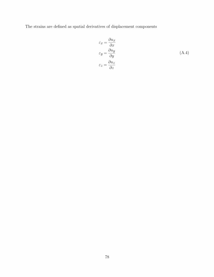
The strains are defined as spatial derivatives of displacement components
εx = ∂ux∂x
εy = ∂uy∂y
εz = ∂uz∂z
(A.4)
78

Appendix B: Relationship between Stiffness Con-stants, Young’s Moduli and Poisson’s Ratios forOrthotropic Materials
The components of stiffness matrix are given in terms of compliances
C11 = (S22S33−S23S23)K
C22 = (S33S11−S13S13)K
(B.1)
C12 = (S13S23−S12S−33)K
C13 = (S12S23−S13S22)K
(B.2)
C33 = (S11S22−S12S12)K
C23 = (S12S13−S23S11)K
(B.3)
C44 = 1S44
C55 = 1S55
C66 = 1S66
(B.4)
K = S11S22S33−S11S23S23−S22S13S13−S33S12S12 + 2S12S23S13 (B.5)
The compliances can be expressed in terms of Young’s moduli and Poisson’s ratios
S11 = 1E1
S12 = −v12E1
S13 = −v13E1
(B.6)
S22 = 1E2
S23 = −v23E2
S33 = 1E3
(B.7)
79

S44 = 1G23
S55 = 1G13
S66 = 1G12
(B.8)
80

BIBLIOGRAPHY
81
BIBLIOGRAPHY
[1] National Transportation Safety Board. Aircraft Accident Report-Aloha Airlines, Flight243, Boeing 737-200, N73711, near Maui, Hawaii, April 28, 1988. NTSB/AAR-89/03,1989.
[2] Crossbow Technology, Inc. IRIS Wireless Measurement System. Document Part Number:6020-0124-01 Rev A, 2010.
[3] K. Diamanti and C. Soutis, Structural Health Monitoring Techniques for Aircraft Com-posite Structures. Progress in Aerospace Sciences, 46:342-352, 2010.
[4] P. C. Chang, A. Flatau andS. C. Liu. Review Paper: Health Monitoring of Civil Infras-tructure. Structural Health Monitoring, 2(3):257-267, 2003.
[5] E. Keller and A. Ray. Real-time Health Monitoring of Mechanical Structures. StructuralHealth Monitoring, 2(3):191-203, 2003.
[6] J. P. Carmo and J. E. Ribeiro. New Advances in Vehicular Technology and AutomotiveEngineering. InTech, 2012.
[7] C. J. Stulla, C. J. Earlsb and P. S. Koutsourelakisb. Model-based Structural Health Mon-itoring of Naval Ship Hulls. Computer Methods in Applied Mechanics and Engineering,200:1137-1149, 2011.
[8] D. Inaudi and B. Glisic. Fiber Optic Sensing for Innovative Oil and Gas Production andTransport Systems. 18th International Conference on Optical Fiber Sensors, 2006.
[9] Crossbow Technology, Inc. Imote2 High-performance Wireless Sensor Network Node.Document Part Number: Document Part Number: 6020-0117-02 Rev A, 2010.
82

[10] S. Stupar, A. Simonovic, M. Jovanovic. Measurement and Analysis of Vibrations onthe Helicopter Structure in Order to Detect Defects of Operating Elements. ScientificTechnical Review, 62:58-63, 2012.
[11] M. Lee, J. Lee and J. Kim. Condition Monitoring of a Nuclear Power Plant CheckValve Based on Acoustic Emission and a Neural Network. J. Pressure Vessel Technol.127(3):230-236, 2005.
[12] H. Lamb, On Waves in an Elastic Plate. Proceedings of the Royal Society, Physical andEngineering Sciences, 93:114-128, 1917.
[13] I. Viktorov. Rayleigh and Lamb Waves: Physical Theory and Applications. Springer,1995.
[14] J. L. Rose. Ultrasonic Waves in Solid Media. Cambridge University Press, 1999.
[15] K. F. Graff. Wave Motion in Elastic Solids. Dover Publications, 1991.
[16] A.H. Nayfeh. Wave Propagation in Layered Anisotropic Media: With Applications toComposites. North Holland, 1995.
[17] V. Giurgiutiu. Structural Health Monitoring with Piezoelectric Wafer Active Sensors.Academic Press, 2008.
[18] http://www.olympus-ims.com/
[19] http://www.ndt.net/
[20] http://www.steminc.com/
[21] An American National Standard. IEEE Standard on Piezoelectricity. ANSI/IEEE Std176-1987, 1988.
[22] A. Bent and N.W. Hagood. Piezoelectric Fiber Composites with Interdigitated Electrodes.Journal of Intelligent Material Systems and Structures, 8 (11):903-919, 1997.
[23] http://www.smart-material.com/MFC-product-main.html
83
[24] E. F. Crawley and J. de Luis, Use of Piezoelectric Actuators as Elements of IntelligentStructures. American Institute of Aeronautics and Astronautics (AIAA), 26:1373-1385,1987.
[25] A. Raghavan and E. S. Cesnik. Finite-dimensional Piezoelectric Transducer Modeling forGuided Wave Based Structural Health Monitoring. Smart. Mater. and Struct., 14(6):1448-1461, 2005.
[26] C. Zhou, Z. Su and L. Chen. Probability-based Diagnostic Imaging Using Hybrid FeaturesExtracted from Ultrasonic Lamb Wave Signals. Smart. Mater. Struct., 20, 2011.
[27] E. Zurich. The Discrete Fourier Transform, Part 4: Spectral Leakage. Journal of ObjectTechnology, 8(7):23-34, 2009.
[28] F. Auger, P. Flandrin, P. Goncalves and O. Lemoine. Time-Frequency Toolbox for Usewith MATLAB., 1996.
[29] V. Giurgiutiu and L. Yu. Comparison of Short-time Fourier Transform and WaveletTransform of Transient and Tone Burst Wave Propagation Signals For Structural HealthMonitoring. 4th International Workshop on Structural Health Monitoring, Stanford Uni-versity, Stanford, CA, September 15-17, 2003.
[30] V. Amaravadi. Structural Health Monitoring Using Wavelet Transform. Smart. Mater.and Struct., 4327:258-269, 2001.
[31] L. De Marchi, A. Marzani, S. Caporale and N. Speciale. A New Warped Frequency Trans-formation (WFT) for Guided Waves Characterization. Health Monitoring of Structuraland Biological Systems, 7295, 2009.
[32] L. Cohen. Time-Frequency Analysis. Prentice Hall, 1995.
[33] D. J. Nelson. Cross-spectral Methods for Processing Speech. J. Acoust. Soc. Am.110(5):2575-2592, 2001.
[34] A. Rihaczek. Signal Energy Distribution in Time and Frequency. IEEE Transactions onInformation Theory. 14:369-384, 1968.
[35] A. V. Oppenheim, R. W. Schafer and J. R. Buck. Discrete-time Signal Processing.Prentice Hall, 1999.
84

[36] L. R. Rabiner and R. W. Schafer. The Chirp-Z Transform. IEEE Transactions on Audioand Electroacoustics. AU-17(2):86-92, 1969.
[37] S.G. Mallat and Z. Zhang. Matching Pursuits with Time-Frequency Dictionaries. IEEETrans. Signal Process. 41:3397-3415, 1993.
[38] B. Xu, V. Giurgiutiu and L. Yu. Lamb Waves Decomposition and Mode IdentificationUsing Matching Pursuit Method. Sensors and Smart Structures Technologies for Civil,Mechanical, and Aerospace Systems. 7292, 2009.
[39] A. Raghavan and C. Cesnik. Guided-wave Signal Processing Using Chirplet MatchingPursuits and Mode Correlation for Structural Health Monitoring. Smart. Mater. Struct.16:255-366, 2007.
[40] Y. Li and J. Michaels. Numerical Implementation of Matching Pursuit for the Analysisof Complex Ultrasonic Signals IEEE Trans. Ultrason. Ferroelectr. Freq. Control. 55:173-182, 2008.
[41] J. C. Hong, K. H. Sun and Y. Y. Kim Waveguide Damage Detection by the MatchingPursuit Approach Employing the Dispersion-based Chirp Functions. IEEE Trans. Ultra-son. Ferroelectr. Freq. Control. 53:592-605, 2006.
[42] A. H. Nayfeh The General Problem of Elastic Wave Propagation in Multilayered Anisotr-pic Media. J. Acoust. Soc. Am. 89(4):1521-1531, 1991.
[43] M. Niethammer and L. J. Jacobs. Time-frequency Representation of Lamb Waves usingthe Reassigned Spectrogram J. Acoust. Soc. Am. 107(5):19-24, 2000.
[44] J. Vishnuvardhan, C Krishnamurthy and K. Balasubramaniam. Genetic Algorithmbased Reconstruction of Elastic Moduli using an Ultrasonic Guided Wave and SingleTransmitter-multiple Receiver SHM Array Systems. Smart. Mater. Struct. 16:1639, 2007.
85