signal classi cation data processing in fluid...

Signal classificationStatistical analysis tools

Data processing in Fluid Mechanics

Data processing

Amelie Danlos, Florent Ravelet

DynFluid Laboratory, Arts et Metiers ParisTech

February 3, 2014

1 Amelie Danlos, Florent Ravelet Experimental methods for fluid flows: an introduction



Signal-to-noise ratioDeterministic signalRandom signalEnergy classification

Outline

1 Signal classificationSignal-to-noise ratioDeterministic signalRandom signalEnergy classification

2 Statistical analysis toolsMomentsCorrelation functionPower Spectral densityExamplesAnalysis of discrete signalsDistribution (generalized function)

3 Data processing in Fluid MechanicsFourier transformFast Fourier transformWindowed Fourier transformWaveletsProper Orthogonal Decomposition





Signal classificationSignal definition: physical quantity measurement recorded from a sensor. Generally, themeasured quantity is an electric voltage.

Signal post-processing consists in analysing statistically the signal in order to highlightmeasured quantity characteristics.

Noise definition: disturbing phenomenon which reduces the result quality.

Noise is a relative notion which depends on the context.

Example: For a telecomunication engineer, satellite waves are the signal while astrophysicalsources provided noise. On the other hand, an astrophysicist considers that astrophysicalsources provided signal and a satellite induces noise.

SIGNAL = Deterministic component + Random component

Signal-to-noise ratio is used to determine the quality of the signal.





Signal-to-noise ratio

RS/N =√

signal mean power√noise mean power

It is often possible to reduce the noise by controlling the environment. Otherwise, when thecharacteristics of the noise are known and are different from the signals, it is possible to filter it orto process the signal. When the signal is constant or periodic and the noise is random, it ispossible to enhance the SNR by averaging the measurement.





Deterministic signalA deterministic signal can be described by analytical expressions for all times (explicitmathematical relations).

This signal is predictable for arbitrarily times and can be reproduced identically arbitrarilyoften

Different types of deterministic signals:

1 Periodic signal

2 Non-periodic signal





Deterministic signalSine-wave signal

Quasi-periodic signal

X (t) = X sin (2πf0t + φ)

X (t) =∑∞

i=1 Xi sin (2πfi t + φi )





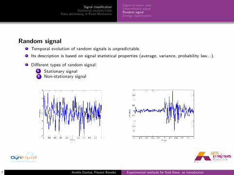
Random signalTemporal evolution of random signals is unpredictable.

Its description is based on signal statistical properties (average, variance, probability law...).

Different types of random signal:1 Stationary signal2 Non-stationary signal





Random signalStationary signalThe ensemble average is defined by:

E (X ) = limN→+∞

1N

∑Ni=1 Xi

The temporal average is defined by:

X = limT→+∞

1T

∫ Ti=0

X (t) dt

Ergodic signal

X = E (X )

Non-ergodic signal

X 6= E (X )

The statistical description of a non-ergodic signal needs the use of ensemble average.





Random signalStationary signal





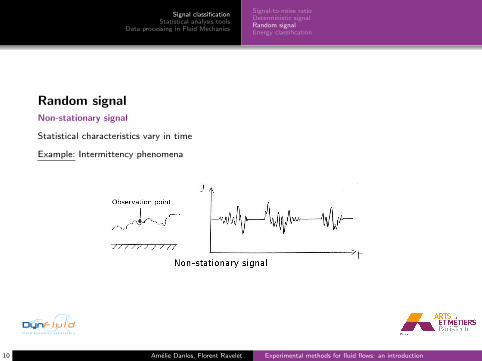
Random signalNon-stationary signal

Statistical characteristics vary in time

Example: Intermittency phenomena





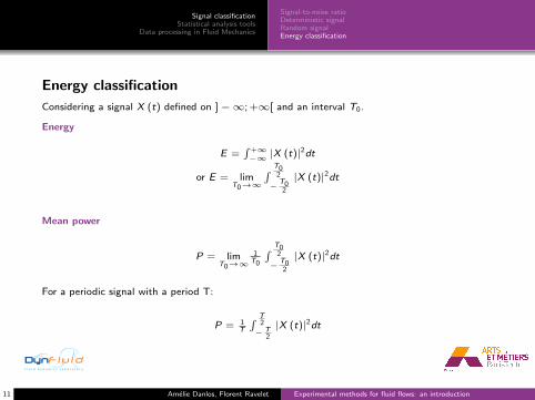
Energy classification

Considering a signal X (t) defined on ]−∞; +∞[ and an interval T0.

Energy

E =∫ +∞−∞ |X (t)|2dt

or E = limT0→∞

∫ T02

− T02

|X (t)|2dt

Mean power

P = limT0→∞

1T0

∫ T02

− T02

|X (t)|2dt

For a periodic signal with a period T:

P = 1T

∫ T2

− T2

|X (t)|2dt





Energy classification

Finite energy signals

⇒ Mean power is null

Infinite energy signals

⇒ Mean power is non-zero

Periodic signals




MomentsCorrelation functionPower Spectral densityExamplesAnalysis of discrete signalsDistribution (generalized function)

Outline








Statistical analysis toolsWe consider now an ergodic stationary signal.

Reynolds statistical decomposition (1894)This decomposition is a mathematical technique to separate the average and fluctuatingparts of a quantity.

X (~a, t) = X (~a) + x (~a, t)

with X the average and x a centered random variable.

The perturbations are defined such that their time average equals zero.

This allows us to simplify the Navier-Stokes equations by substituting in the sum of thesteady component and perturbations to the velocity profile and taking the mean value. Theresulting equation contains a nonlinear term known as the Reynolds stresses which gives riseto turbulence.

Different statistical quantities can be obtained from this signal.





MomentsFirst order moment: Mean

X = limT→∞

1T

∫ T

0X (t) dt

This statistical operator reports the studied quantity X by abstracting its temporal variations x .

Second order moment: Variance

x2 = limT→∞

1T

∫ T0

x2 (t) dt

This quantity represents the energy of the variable x .

We use preferably the Root Mean Squared value (RMS), which is the square root of thevariance:

σ (x) =√

x2





Probability Density Function (PDF)

PDF is a function that describes the relative likelihood for this random variable to take on agiven value.

The probability for the random variable to fall within a particular region is given by theintegral of this variable’s density over the region.

The probability density function is positive everywhere.

Its integral over the entire space is equal to one.

We call p (X ) the probability density function of X such as:

X =∫ +∞−∞ ξp (ξ) dξ

For a centered random variable, we have: x =∫ +∞−∞ ηp (η) dη = 0

The second order moment is: x2 =∫∞−∞ ξ2p (ξ) dξ

Then the probability density function verifies:

p (x) ≥ 0∫ +∞−∞ p (ξ) dξ = 1

This function is also called first order moment of probability density function.





Probability Density Function (PDF)

In Fluid Mechanics, numerous phenomena are described by a gaussian probability densitywhich follows:

p (x) = 1σ(x)√

2πe− x2

2σ2(x)

For two random functions x and y , we define the second order moment of probabilitydensity function p (x, y):

xy =∫ +∞−∞

∫ +∞−∞ ξηp (ξ, η) dξdη





MomentsThird order moment: Skewness

x3 = limT→∞

1T

∫ T0

x3 (t) dt or x3 =∫ +∞−∞ ξ3p (ξ) dξ

Any symmetric distribution will have a third central moment of zero.

A distribution that is skewed to the left (the tail of the distribution is heavier on the left)will have a negative skewness.

A distribution that is skewed to the right (the tail of the distribution is heavier on the right),will have a positive skewness.

The skewness coefficient is:

S = x3

(x2)32

For a gaussian signal: S = 0





MomentsFourth order moment: Flatening coefficient or Kurtosis

x4 = limT→∞

1T

∫ T0

x4 (t) dt or x4 =∫ +∞−∞ ξ4p (ξ) dξ

Flatening coefficient or Kurtosis: T =¯x4(¯x2)2

For a gaussian signal: T = 3





Correlation functionA correlation function is the correlation between random variables at two different points inspace or time, usually as a function of the spatial or temporal distance between the points.

If one considers the correlation function between random variables representing the samequantity measured at two different points then this is often referred to as an autocorrelationfunction.

Correlation functions of different random variables are sometimes called cross correlationfunctions to emphasise that different variables are being considered.

Correlation functions are a useful indicator of dependencies as a function of distance in timeor space, and they can be used to assess the distance required between sample points for thevalues to be effectively uncorrelated. In addition, they can form the basis of rules forinterpolating values at points for which there are observations.





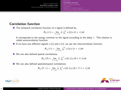
Correlation functionThe temporal correlation function of a signal is defined by:

Rxx (τ) = limT→∞

1T

∫ T0

x (t) x (t + τ) dt

It corresponds to the energy common to the signal according to the delay τ . This relation iscalled autocorrelation function.

If we have two different signals x (t) and y (t), we use the intercorrelation function:

Rxy (τ) = limT→∞

∫ T0

x (t) y (t + τ) dt

We can also defined spatial correlations:

Rxy (~r) = limT→∞

1T

∫ T0

x (~a, t) y (~a +~r , t) dt

We can also defined spatiotemporal correlations:

Rxy (~r , τ) = limT→∞

1T

∫ T0

x (~a, t) y (~a +~r , t + τ) dt





Correlation coefficientThe correlation coefficient is built from the correlation function:

CRxx (τ) = Rxx (τ)

σ2(x)

CRxy (τ) =Rxy (τ)

σ(x)σ(y)





Power Spectral density

In statistical signal processing and physics, the spectral density, power spectral density(PSD), or energy spectral density (ESD), is a positive real function of a frequency variableassociated with a stationary stochastic process, or a deterministic function of time, whichhas dimensions of power per hertz (Hz), or energy per hertz.

It is often called simply the spectrum of the signal. Intuitively, the spectral density measuresthe frequency content of a stochastic process and helps identify periodicities.

This function is defined from the correlation function:

Sxx (f ) =∫ +∞−∞ Rxx (τ) e−2πif τdτ

where the Fourier transform of x (t) is:

x (f ) =∫ +∞−∞ x (t) e−2πiftdt

This function represents the energy distribution of a signal according to the frequency. Thenthe total energy can be provided by the integration of the spectral density:

x2 =∫ +∞−∞ Sxx (f ) df

The interspectral power density of two signals is defined as:

Sxy (f ) =∫ +∞−∞ Rxy (τ) e−2πif τdτ





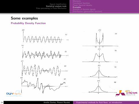
Some examplesProbability Density Function





Some examplesAutocorrelation Function





Some examplesPower Spectral Density





Analysis of discrete signals

Nyquist-Shannon sampling theorem

Sampling is the process of converting a signal (for example, a function of continuous time orspace) into a numeric sequence (a function of discrete time or space).

Then the sufficient condition for exact reconstructability from samples at a uniformsampling rate fs (in samples per unit time) is:

fs > 2B where B is the bandwidth.





Analysis of discrete signals

Temporal averageConsidering a signal sampling in Ne points at a frequency fe = 1

∆t .

X (~a) = 1Ne

∑Nei=1 X (~a, i∆t)

If we write Xi the sampled values in the moments i∆t, we obtain:

X = 1Ne

∑Nei=1 Xi

MomentsIf we consider a signal Xi = X + xi :

x2 = 1Ne

∑Nei=1 x

2i

x3 = 1Ne

∑Nei=1 x

3i

x4 = 1Ne

∑Nei=1 x

4i





Distribution (generalized function)In mathematical analysis, distributions (or generalized functions) are objects that generalizefunctions. Distributions make it possible to differentiate functions whose derivatives do notexist in the classical sense. In particular, any locally integrable function has a distributionalderivative.

Distributions are also important in physics and engineering where many problems naturallylead to differential equations whose solutions or initial conditions are distributions, such asthe Dirac distribution.

If φ is a function the Dirac distribution or Dirac impulse is defined by:

δ (φ) =∫ +∞−∞ φ (t) .δ (t) dt = φ (0)

Dirac distribution represents a signal with a duration theoretically null and a finite energyE = 1.





Distribution (generalized function)Dirac comb

In mathematics, a Dirac comb (also known as an impulse train and sampling function inelectrical engineering) is a periodic Schwartz distribution constructed from Dirac deltafunctions

∆T (t) =∑+∞

k=−∞ δ (t − kT )

Because the Dirac comb function is periodic, it can be represented as a Fourier series:

∆T (t) = 1T

∑+∞n=−∞ e i2πnt/T





Distribution (generalized function)Properties:

D (φ1 + φ2) = D (φ1) + D (φ2)

D (λφ) = λD (φ)

where λ is a scalar.

Distribution derivation:

D′ (φ) = −D(φ′)




Fourier transformFast Fourier transformWindowed Fourier transformWaveletsProper Orthogonal Decomposition

Outline








This part deals with some fundamental transforms and analysis procedures commonly used forboth signal and data processing in fluid mechanics measurements.

Data processing in Fluid Mechanics:

Fourier Transform

Fast Fourier Transform

Windowed Fourier Transform

Wavelets

Proper Orthogonal Decomposition

Phase averaging





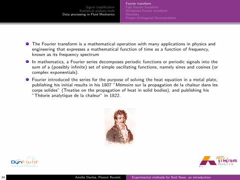
The Fourier transform is a mathematical operation with many applications in physics andengineering that expresses a mathematical function of time as a function of frequency,known as its frequency spectrum

In mathematics, a Fourier series decomposes periodic functions or periodic signals into thesum of a (possibly infinite) set of simple oscillating functions, namely sines and cosines (orcomplex exponentials).

Fourier introduced the series for the purpose of solving the heat equation in a metal plate,publishing his initial results in his 1807 ”Memoire sur la propagation de la chaleur dans lescorps solides” (Treatise on the propagation of heat in solid bodies), and publishing his”Theorie analytique de la chaleur” in 1822.





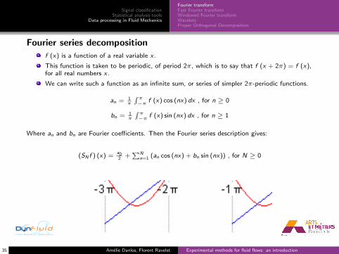
Fourier series decomposition

f (x) is a function of a real variable x .

This function is taken to be periodic, of period 2π, which is to say that f (x + 2π) = f (x),for all real numbers x .

We can write such a function as an infinite sum, or series of simpler 2π-periodic functions.

an = 1π

∫ π−π f (x) cos (nx) dx , for n ≥ 0

bn = 1π

∫ π−π f (x) sin (nx) dx , for n ≥ 1

Where an and bn are Fourier coefficients. Then the Fourier series description gives:

(SN f ) (x) =a02 +

∑Nn=1 (an cos (nx) + bn sin (nx)) , for N ≥ 0





Fourier series decomposition

We have also:

f (x) =∑+∞

n=−∞ cneinx

with: cn = 12π

∫ π−π f (x) e−inxdx the Fourier coefficients

Even for a real function x (t), the Fourier coefficients are complex values.

The usual interpretation of this complex number is that it gives both the amplitude (or size)of the wave present in the function and the phase (or the initial angle) of the wave.

Thus, the real part represents contributions to the signal, which are symmetric about zeroand the imaginary part describes the asymmetric contributions.

These complex exponentials sometimes contain negative ”frequencies”. Hence, frequency nolonger measures the number of cycles per unit time, but is still closely related.





Fourier transform

The Fourier transform (FT) is an integral transform with orthogonal sinusoidal basisfunctions of different frequencies.

The result represents the frequency spectrum of the signal.

For a continuous complex signal x (t) with finite energy content the superposition of theFourier series becomes:

x (t) =∫ +∞−∞ X (f ) e2πiftdf

with: X (t) =∫ +∞−∞ x (f ) e−2πiftdt

Signal with finite energy fulfill∫ +∞−∞ |x (t) |dt <∞

This implies that the signal is nonperiodic.

The result of the decomposition X (f ) is called the Continuous Fourier transform (CFT).

It is a continuous, infinite, non-periodic, complex frequency spectrum, which fulfills thePlancherel theorem, indicating the conservation of energy by the Fourier transform:∫ +∞

−∞ |X (f ) |2df =∫ +∞−∞ |x (t) |2dt





Fourier transform

Considering a finite series of complex values xn = x (t = n∆ts ) with n = 0, 1, . . . ,N − 1,sampled at equal time intervals over the time duration T = N∆ts , the Discrete FourierTransform (DFT) resulting from the decomposition into a finite sum of complex Fouriercoefficients Xk is defined as:

Xk = X (f = k∆f ) = FT (xn) =∑N−1

n=0 xn exp(−i 2πnk

N

)with k = 0, 1, . . . ,N − 1

The inverse transform is:

xn = FT−1 (Xk ) = 1N

∑N−1n=0 Xk exp

(+i 2πnk

N

)with n = 0, 1, . . . ,N − 1

The frequency spacing of the resulting Fourier coefficients (it is also the lowest frequencythat can be resolved) is defined as:

∆fs = 1N∆ts

= 1T = fs

N .





Fourier transform

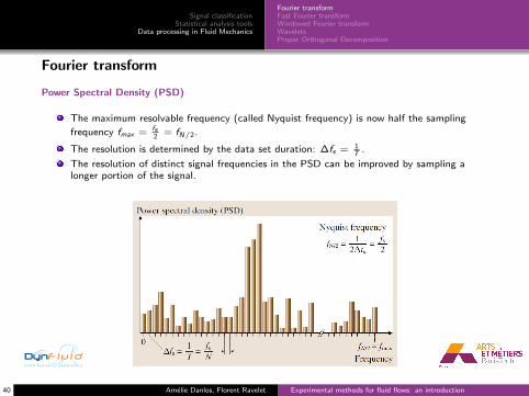
Power Spectral Density (PSD)

The Power Spectral Density (PSD) is given by the squared magnitude of the spectralcoefficients:

Sk = S (f = fk ) = 1Nfs|Xk |2 with k = 0, 1, . . . ,N − 1

This function represents the distribution of the total signal power between the frequencies 0and fs .

The PSD is symmetric about k = N2 and has a periodicity every N samples. Therefore, an

alternative representation is the use of negative and positive frequencies. For this case, allvalues of k ≥ N

2 are interpreted as negative frequency values and the spectrum is symmetricabout k = 0.

The spectral distribution between k = 0 and k = N2 is defined as:

Gk = 2N2∆fs

X∗k Xk with k = 0, 1, . . . , N2





Fourier transform

Power Spectral Density (PSD)

The maximum resolvable frequency (called Nyquist frequency) is now half the sampling

frequency fmax = fs2 = fN/2.

The resolution is determined by the data set duration: ∆fs = 1T .

The resolution of distinct signal frequencies in the PSD can be improved by sampling alonger portion of the signal.





Fourier transform





Fourier transform

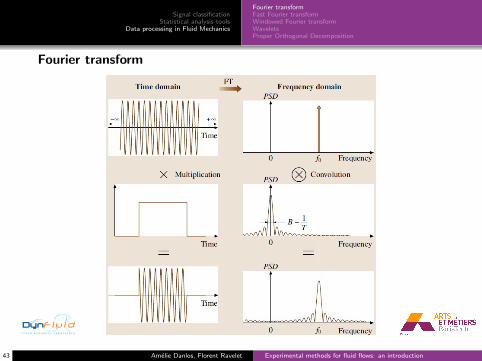
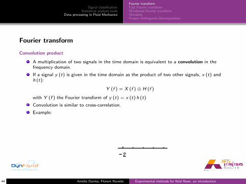
Convolution product

A multiplication of two signals in the time domain is equivalent to a convolution in thefrequency domain.

If a signal y (t) is given in the time domain as the product of two other signals, x (t) andh (t):

Y (f ) = X (f )⊗ H (f )

with Y (f ) the Fourier transform of y (t) = x (t) h (t)

Convolution is similar to cross-correlation.

Example:





Fast Fourier Transform

A fast Fourier transform (FFT) is an efficient algorithm to compute the discrete Fouriertransform (DFT) and its inverse.

Invented by Cooley and Tukey in 19651

There are many distinct FFT algorithms involving a wide range of mathematics, from simplecomplex-number arithmetic to group theory and number theory.

All these algorithms normally operate on 2n points.

The FFT algorithm reduces the computation time to the order of N log10 N.

1Cooley J.W., Tukey J.W.,”An algorithm for the machine calculation of complex Fourier series”,Math.Comput.,19:297-301,1965





Fourier TransformCorrelation function

The power spectral density S is related to the autocorrelation function R (Wiener-Khinchinerelation):

S (f ) = FTR (τ) =∫ +∞−∞ R (τ) dτ

R (τ) = FTS (f ) =∫ +∞−∞ S (f ) dτ

For a sampled signal:

Sk = 1fs

∑N−1n=0 Rn exp

(−i 2πkn

N

)Rn = fs

N

∑N−1k=0 Sk exp

(+i 2πkn

N

)





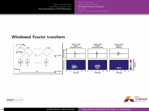
Windowed Fourier transform

Clearly the Fourier spectrum is not the best analysis tool for signals whose spectra fluctuatein time.





Windowed Fourier transformOne solution to this problem is the so-called ”Short-time Fourier Transform” or ”WindowedFourier Transform” (WFT) in which we can compute the Fourier spectra using a slidingtemporal window. By adjusting the width of the window we can determine the timeresolution of the resulting spectra.

Other alternative tools are the Wigner transform, the Continuous Wavelet Transform(CWT), and the Discrete Wavelet Transform (DWT).





Windowed Fourier transform





WaveletsA wavelet is a wave-like oscillation with an amplitude that starts out at zero, increases, andthen decreases back to zero.

The word wavelet has been used for decades in digital signal processing. The equivalentFrench word ondelette meaning ”small wave” was used by Morlet and Grossmann in theearly 1980s.

A Continuous Wavelet Transform (CWT) is used to divide a continuous-time function intowavelets.

Unlike Fourier transform, the continuous wavelet transform possesses the ability to constructa time-frequency representation of a signal that offers very good time and frequencylocalization.





WaveletsThe continuous wavelet transform of a continuous, square-integrable function x (t) at ascale a > 0 and translational value b ∈ R is expressed by the following integral:

X (a, b) = 1√|a|

∫ +∞−∞ x (t)ψ∗

(t−ba

)dt

where ψ (t) is a continuous function in both the time domain and the frequency domaincalled the mother wavelet.

The main purpose of the mother wavelet is to provide a source function to generate thedaughter wavelets which are simply the translated and scaled versions of the mother wavelet.To recover the original signal x (t), inverse continuous wavelet transform can be exploited:

x (t) =∫ +∞

0

∫ +∞−∞

1a2 W (a, b) 1√

|a|ψ(

t−ba

)db da

where ψ (t) is the dual function of ψ (t).

The dual function should satisfy:∫ +∞0

∫ +∞−∞

1|a3|

ψ(

t1−ba

)ψ(

t−ba

)db da = δ (t − t1)





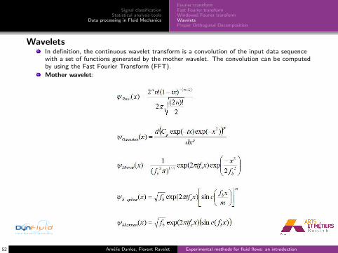
WaveletsIn definition, the continuous wavelet transform is a convolution of the input data sequencewith a set of functions generated by the mother wavelet. The convolution can be computedby using the Fast Fourier Transform (FFT).

Mother wavelet:





WaveletsA Discrete Wavelet Transform (DWT) is any wavelet transform for which the wavelets arediscretely sampled.It captures both frequency and location information (location in time).The first DWT was invented by the Hungarian mathematician Alfred Haar.





Wavelets





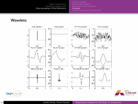
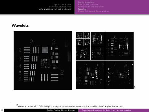
Wavelets

2

2Verrier N., Atlan M., ”Off-axis digital hologram reconstruction: some practical considerations”,Applied Optics,2011.





Wavelets





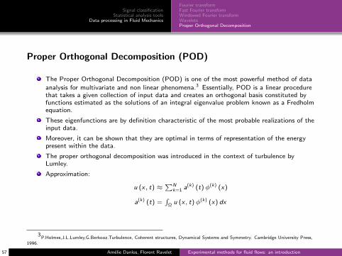
Proper Orthogonal Decomposition (POD)

The Proper Orthogonal Decomposition (POD) is one of the most powerful method of data

analysis for multivariate and non linear phenomena.3 Essentially, POD is a linear procedurethat takes a given collection of input data and creates an orthogonal basis constituted byfunctions estimated as the solutions of an integral eigenvalue problem known as a Fredholmequation.

These eigenfunctions are by definition characteristic of the most probable realizations of theinput data.

Moreover, it can be shown that they are optimal in terms of representation of the energypresent within the data.

The proper orthogonal decomposition was introduced in the context of turbulence byLumley.

Approximation:

u (x, t) ≈∑N

k=1 a(k) (t)φ(k) (x)

a(k) (t) =∫

Ωu (x, t)φ(k) (x) dx

3P.Holmes,J.L.Lumley,G.Berkooz.Turbulence, Coherent structures, Dynamical Systems and Symmetry. Cambridge University Press,

1996.





Other methods to study coherent structures of turbulent flows

Phase averaging

Finite-Time Lyapounov Exponent (FTLE)

Dynamic Mode Decomposition

. . .


signal classi cation data processing in fluid...

Documents