signal coupling and signal integrity in multi-strip resistive plate chambers used for timing...
TRANSCRIPT

Nuclear Instruments and Methods in Physics Research A 648 (2011) 52–72
Contents lists available at ScienceDirect
Nuclear Instruments and Methods inPhysics Research A
0168-90
doi:10.1
� Corr
German
E-m
journal homepage: www.elsevier.com/locate/nima
Signal coupling and signal integrity in multi-strip resistive plate chambersused for timing applications
Diego Gonzalez-Diaz a,b,c,�, Huangshan Chen b, Yi Wang b
a GSI Helmholtzcenter for Heavy Ion Research, Darmstadt, Germanyb Technical University, Darmstadt, Germanyc Department of Engineering Physics, Tsinghua University, Beijing, China
a r t i c l e i n f o
Article history:
Received 13 December 2010
Received in revised form
13 April 2011
Accepted 15 May 2011Available online 25 May 2011
Keywords:
RPC
Time-of-flight
Multi-strip RPC
Multi-hit capability
Cross-talk
Electrically long counters
Simulations
Inhomogeneous transmission lines
02/$ - see front matter & 2011 Elsevier B.V. A
016/j.nima.2011.05.039
esponding author at: GSI Helmholtzcenter for H
y.
ail address: [email protected] (D. Gonz
a b s t r a c t
We have systematically studied the transmission of electrical signals along several 2-strip Resistive
Plate Chambers (RPCs) in the frequency range f ¼ 0:1�3:5 GHz. Such a range was chosen to fully cover
the bandwidth associated to the very short rise-times of signals originated in RPCs used for sub-100 ps
timing applications. This work conveys experimental evidence of the dominant role of modal dispersion
in counters built at the 1 m scale, a fact that results in large cross-talk levels and strong signal shaping.
It is shown that modal dispersion appears in RPCs due to their inherent unbalance between capacitive
and inductive coupling. A practical way to restore this symmetry has been introduced (hereafter
‘electrostatic compensation’), allowing for a cross-talk suppression factor up to �12 and a rise-time
reduction by 200 ps. Under conditions of compensation the signal transmission is only limited by
dielectric losses, yielding a length-dependent cutoff frequency of around 1 GHz for propagation along
2 m in typical float glass-based RPCs.
It is further shown that ‘electrostatic compensation’ can be achieved for an arbitrary number of
strips as long as the nature of the coupling is ‘short-range’, that is an almost exact assumption for
typical strip-line RPCs. This work extends the bandwidth of previous studies by a factor of�20.
& 2011 Elsevier B.V. All rights reserved.
1. Introduction
Cross-talk and signal integrity are, a priori, critical aspects forthe operation of electrically long Resistive Plate Chambers (RPCs)with readout based on multi-segmented electrodes. The some-times called multi-strip multi-gap RPCs (MMRPCs in short),pioneered by the 4p-experiment [1] at GSI fall, exemplarily, intothis (by no means small) category. In order to streamline theforthcoming discussion some preliminary considerations arenecessary. We will first introduce, as in Refs. [2,3], the electricallength Le of a resistive plate chamber. This is done based on the‘cutoff frequency’ of the current induced by a single-electronavalanche in the absence of space-charge effects and at typicalworking conditions:
IðtÞ ¼ I0eStyðtÞ ð1Þ
jftðIðtÞÞj ¼I0ffiffiffiffiffiffiffiffiffiffiffiffiffiffiffiffiffiffiffiffiffiffiffi
ð2pf Þ2þS2
q ð2Þ
ll rights reserved.
eavy Ion Research, Darmstadt,
alez-Diaz).
where yðtÞ represents the Heaviside step function, ‘ft’ denotes theFourier transform, J refers to the modulus of the bracketed complexfunction, and S¼ ða�ZÞvdrift stands for the ionization rate in theactive gas. The latter serves as a definition, in the present context, ofa and Z (the multiplication and attachment coefficients, respec-tively) and vdrift (the drift velocity of the electron swarm). Curiously,since no assumption is made on the sign of S, Eq. (2) is obviouslyidentical to the modulus of the response function of a low-passRC-circuit with S¼�1=RC.
The ‘cutoff frequency’ of a signal, fc, is defined as the frequencyneeded for a drop by a factor of 1=
ffiffiffi2p
(i.e., �3 dB) in its Fourieramplitude spectra with respect to the DC/zero-frequency limit;also often equivalently defined as the frequency needed for afactor 1/2 drop in the Fourier power spectra. This yields thusfc ¼ S=2p from Eq. (2). Assuming, with sufficient generality forpresent purposes, that signal propagation takes place at approxi-mately half the speed of light, the electrical length of an RPC oflength D can be estimated as
Le ¼D
lc¼
fc
vDC
S
pcD ð3Þ
where v is the signal propagation velocity, c is the speed of lightand D is the counter length.

D. Gonzalez-Diaz et al. / Nuclear Instruments and Methods in Physics Research A 648 (2011) 52–72 53
With approximate character, an electrically long structure iscustomary defined as that fulfilling the condition Le41 [3]. Thisrepresents a standard engineering figure telling when a circuitaldescription is no longer possible and signal transmission must beconsidered explicitly in the problem. For time-pulses (the casediscussed here), where a continuous frequency-spectrum ispresent, a more conservative ‘rule of thumb’ is sometimes givenas Le41=10, where Le is determined as in Eq. (3). According toRef. [3], if the above condition is fulfilled, circuit theory must beabandoned.
It is possible to quantitatively understand the implication of theabove fact thanks to the recently measured parameters of theswarm [4] for the main RPC gas component (C2H2F4). Thesemeasurements were performed at low-pressure and are thus largelyfree of saturation effects, corresponding approximately to thesituation sketched in Eq. (1). When extrapolated to typical workingconditions (T¼20 1C, P¼1 atm), the parameters measured in Ref. [4]provide the following lower bounds for the length Dn above whichan RPC becomes electrically long:
Dn
triggerðE¼ 50 kV=cmÞ ¼pc
SðE¼ 50 kV=cmÞ¼ 80 cm ð4Þ
Dn
timingðE¼ 100 kV=cmÞ ¼pc
SðE¼ 100 kV=cmÞ¼ 5 cm: ð5Þ
Eqs. (4) and (5) have been evaluated for two typical field valuescorresponding to RPCs used for trigger, EC50 kV=cm [5] andtiming, EC100 kV=cm [6]. In particular, the cutoff frequencyobtained for timing RPCs is as high as fc C3 GHz. The signalbandwidth is thus reasonably met by the fast front end electronicsused in the so far existing strip timing RPC walls from the4p-experiment [7] (BW C1:5 GHz) and HADES [8] (BWC2 GHz).More realistically, rise-time measurements performed directly overRPC signals with a 2-stage � 2 GHz-bandwidth amplifier at typicalpressure, gas mixture and HV, as in Ref. [9], have yielded a value offc¼1.4 GHz at 100 kV/cm. The 1/2 lower signal bandwidth ascompared to the one from Ref. [4] may be interpreted as acontribution of both the presence of space-charge for typical work-ing thresholds and the limited bandwidth of the readout system, ashas been argued by authors [10].1
It is thus expected, on very general grounds, that extremeconditions for signal transmission take place, most prominently, inthe 0.9 m-long multi-strip wall of the 4p-experiment [1] (Le ¼ 18),the 1.6 m-long 2-strip counter developed by Fonte in 2002 [11] and,more recently, in the 1.6 m-long counters of the EEE project [12](both Le ¼ 32).2 Second generation multi-strip counters likeCBM-ToF [13], R3B-neuLAND [14], R3B-iTOF [15] or the STAR-MTDupgrade [16] are presently planned to be built based on multi-stripdesigns with lengths in the range 0.5–2 m (Le ¼ 10240). Althoughsingle-strip designs like the HADES time-of-flight (ToF) wall offer asafe alternative from the point of view of signal transmission, beingvirtually cross-talk free [17], it is at present questionable whethersuch an approach is practical for large numbers of cells, in view ofthe ‘manpower� time’ overhead.
Of the above experiments, genuine multi-hit environmentslike CBM (3–5% occupancy per strip per event, C1000 tracks perevent), speak against large cluster sizes that may typically ariseeither during signal induction or due to sustained capacitive and
1 The estimate of fc from the signal rise-time is not affected by a mere
bandwidth reduction of the measuring device as long as the signal is purely
exponential. This has been shown in Ref. [9] for lineal devices. Deviations from
the exponential growth at the discrimination point are thus needed in order to
reduce fc.2 The HADES wall is not included in this list due to its single-strip design, that
makes signal transmission a far simpler problem. HADES longest strip is
Le C11-long.
inductive coupling during signal transmission over many elec-trical lengths, i.e., cross-talk. Efficiency measurements on the2-strip, 1.6 m-long prototype of [11] point, indeed, to very highcross-talk levels (80–90%) while the 4p-experiment has recentlyreported a cluster size of the order of 4.5 strips/track [18]. There isadditional evidence that the cluster sizes measured in the earliercase are generated indeed during signal transmission [2] whilethe ones measured in the latter have certainly a sizable contribu-tion from the avalanche foot-print (see next section). Remarkably,it has been shown by the EEE collaboration that reducing thesystem bandwidth from fc C3 GHz to C300 MHz (amplifierpeaking time C1 ns), i.e., a � 1=10 bandwidth reduction, iscompatible with preserving a good time resolution and efficiencyfor long strips, thus largely relaxing condition (5) by approxi-mately the same factor and easing transmission.3 Yet, the lowfilling factor (strip to pitch ratio) of less than 80% used in thosecounters [12] (presumably stemming from cross-talk optimization)together with the observed position-dependent space resolutionalong the strips do not ensure the uniformity of response; theabsence of experimental information on the shear cross-talk levelsand cluster sizes do not allow to take a good multi-hit performancefor granted, either. Thus, none of these scenarios seem to betechnologically satisfactory for a high multiplicity experiment like,for instance, CBM.
Besides the aforementioned developments, systematic studieson signal propagation in RPCs are very limited. Numericalsimulations have been performed for the Pestov counter [19]while systematic measurements are available for trigger-typeRPCs [20], where the main phenomena ruling signal coupling inmulti-strip counters have been unambiguously identified. Thework of Riegler in 2002 [21], combining experimental observa-tions and simulations, remains possibly the most complete up todate, despite covering a modest 200 MHz bandwidth and beingperformed for trigger-type RPCs. Not only cross-talk but alsospecially dielectric losses (due to the presence of float glass)remain thus to be assessed in timing-type RPCs up to fc C3 GHz.
This work is structured as follows: in Section 2, we discusscluster sizes in multi-strip RPCs, identifying the contributions fromthe avalanche induction profile (charge sharing) and from the signaltransmission (cross-talk). In Section 3, we present systematic pulser/scope-based measurements of transmission properties for 2-stripRPCs; based on the structure of the solutions for the loss-lesstransmission line problem [21], a novel scheme for cross-talkcompensation in RPCs is introduced. In Sections 4 and 5, we discussthe generalization of this concept to lossy N-strip systems. For that,in Section 4, we identify the dielectric losses by measuring the RPCfrequency response with a large bandwidth network analyzer, givinga simple theoretical prescription on how to include them into theloss-less solutions. Following, in Section 5, an extension of theaforementioned compensating scheme is given for N-strips, withparticular focus on the literal solutions for 5-strip structures.A discussion on the results and the conclusions of the work aregiven in Sections 6 and 7.
2. Cluster sizes in multi-strip RPCs
Large cluster sizes either restrict the track identificationcapability of a time-of-flight detector or proportionally increaseits cost. This is so because conceptual designs of this type ofdetectors, unlike tracking detectors, are usually based on theaverage system occupancy as their main figure of merit. The latter
3 As recalled in an earlier footnote, this statement is dependent, in detail, on
the signal shape.

5 For instance, the theorems obtained in Ref. [24] predict an equal signal
sharing for infinite strips placed over an infinite floating conductor. However, any
signal registered on the strips placed at infinite can only arrive after an infinite
time, since the induction cannot take place faster than the speed of light.
D. Gonzalez-Diaz et al. / Nuclear Instruments and Methods in Physics Research A 648 (2011) 52–7254
is nothing else but the average probability that a detection cell/strip is hit per event, thus the ratio of the average number oftracks per event to the number of active cells n ¼Ntracks=Ncells. Fora Poisson-distributed track multiplicity, the fraction of cells perevent over which more than one track will imping can becalculated simply as
P41 ¼ 1�P0�P1 ¼ 1�ð1þnÞe�n ð6Þ
assuming that each track produces a measurable signal in onlyone cell. The probability of finding a cell with more than one hit(P41) amongst all the fired cells is usually referred to as the‘double hit probability’:
Pdouble ¼P41
P1þP41¼
1�ð1þnÞe�n
1�e�nCn ð7Þ
where the assumption n51 has been made to derive the right-hand-side identity. Very often it is not possible to identify any of thetwo tracks arriving at the same cell so 2Pdouble represents, approxi-mately, the contamination from wrongly identified tracks thatunavoidably goes into the physics analysis (or the track-matchinginefficiency, in case tracks hitting those cells are discarded). Once anacceptable value for Pdouble is fixed by the physics goals (for instance,5%), preliminary cost estimates can be performed (in approximatelinear proportionally with the number of required cells).
In the more realistic case where each track causes in average acertain number of strips to fire (ns),
4 Eq. (7) must be replaced by
Pdouble ¼
1� 1þNtracks
Ncellsns
� �e�ðNtracks=NcellsÞns
1�e�ðNtracks=NcellsÞns: ð8Þ
The number of cells required for keeping Pdouble close to a certaindesign value in an environment with a given number of tracksincreases, thus, in direct proportionality with the cluster size,unless an increase of Pdouble as a function of ns, according toEq. (8), is accepted. Besides the shear occupancy problem, a trackcrossing a timing RPC may affect more than just ns strips. Theelectromagnetic perturbation on the strips potential, even ifbelow threshold, can affect the time measured for a coincidenttrack in an uncontrolled way. This possibility has been studied sofar, perhaps strikingly, only for single-strip structures [17,28]where the effect should be absent. Even in these almost idealconditions, a slight degradation of the time resolution could stillbe seen in Ref. [17] affecting the first neighbors’ performanceunder multi-hit conditions, despite the cross-talk levels were assmall as 0.4%.
A priori, the most obvious candidate for increasing the RPCcluster sizes is the spatial spread of the avalanche charge.Although no experimental value for the transverse diffusioncoefficient DT exists for the standard RPC gas mixture, an estimatecan be made based on the one recently measured for the long-itudinal diffusion coefficient DL in pure C2H2F4 [4] by using theansatz DT CDL, that is a good approximation at high fields. Thisyields an avalanche diffusion radius r¼
ffiffiffiffiffiffiffiffiffiffiffiffiffiffiffiffiffiffiffi2DT g=vd
pC15 mm for a
gap g¼0.3mm under E¼100 kV/cm (and rC40 mm for g¼2 mm,E¼50 kV/cm). Given the typical transverse scale of the readoutstrips (� cm), the avalanche diffusion can be thus expected tohave a very minor role, indeed, in the observed cluster sizes.
Experimentally first [20] and later theoretically [21–24], thetwo main electrostatic effects that can dominate the cluster sizesand the signal shapes in multi-strip RPCs have been identified.Following [24], in the next subsection we discuss, semi-quantita-tively, cluster sizes originated from the induction process.
4 This is, incidentally, the definition of cluster size.
2.1. Charge sharing
In the most general case nowadays, where the high voltage(HV) is applied through a low-conductive coating of surfaceresistivity Rs (for instance [25]), four paradigmatic situations canoccur from the point of view of signal induction (Fig. 1):
(1)
6
whic
depe
The characteristic avalanche duration time tavCg=vd is muchlarger than the response time of the HV coating tHV underwhich the latter behaves in practice like a perfect conductor(tavC1:5 ns for g¼0.3 mm, E¼100 kV; tavC18 ns forg¼2 mm, E¼50 kV, as from Ref. [4]). The induction can beseen as taking place on the HV electrode (see left dottedcurrent generator in Fig. 1-up-left) that is capacitivelycoupled to the readout strips in a high-pass configuration.When the coupling between HV and readout strips is ideal(Cins ¼1) all the strips see the same signal, proportional tothe counter capacitance per unit area CA divided by thenumber of strips.
(2)
The characteristic avalanche duration time tav is muchsmaller than tHV . The avalanche induces currents in theelectrodes according to the ‘weighting fields’ Ew obtainedupon application of the Ramo theorem [26]. The weightingfields determined in that way can still, in specific geometries,cause sizeable cluster sizes (for instance, Fig. 2-left).(3)
For completeness, an abstraction can be made on case (i), byimposing the additional condition that the coating representsan ideal ground (a situation not obviously realizable inpractice). In this case, the signal disappears at the coating,by definition, thus screening the readout strips completely.(4)
At last we can consider the avalanche duration to be compar-able to tHV (intermediate situation). A time-dependentweighting field must be then calculated. A simple prescriptionis given in Ref. [24] on how to do this, together with practicalexamples for 1-gap chambers. As simple as it may be, noattempt has been made, so far, to verify this model.It is important to realize an implicit assumption made in Ref.[24], and thus in cases (i)–(iv): the region affected by theinduction process rind must be electrically short rindr5 cm (fromEq. (5)). Otherwise, field propagation must be obviously takeninto account. This fact highlights the difficulty of addressing cases(i) and (iii) in a practical situation, given an arbitrary number ofstrips.5 For the geometries discussed here, however, and for mostpractical cases, it is reasonable to assume that rindr5 cm (see forinstance the weighting field profiles obtained in two extremescenarios in Fig. 2).
Under the, usually desired, condition tav5tHV , the cluster sizeoriginated during induction is the smallest possible and can beobtained from the static weighting field profile determined withthe Ramo theorem alone (case (ii)). This situation is often given inpractice. In order to better understand the implications of thiscondition, we take the expression for tHV obtained in Ref. [24]:
tHV CRse0h ð9Þ
where h can be interpreted as the anode–cathode distance, e0 isthe electric permittivity of the empty space and Rs is the surfaceresistivity of the material in O=&.6 We take, for illustration, a
This expression is exact only for 1-gap chambers without resistive plates, for
h the problem could be analytically solved in Ref. [24]. Since (i) the time-
ndent component of the weighting field is exponentially suppressed with tHV

−8 −6 −4 −2 0 2 4 6 8
0
0.2
0.4
0.6
0.8
1
x [mm]
Ew [m
m−1
]
4π−experiment
−40 −30 −20 −10 0 10 20 30 40
0
0.1
0.2
0.3
0.4
0.5
0.6
0.7
x [mm]
Ew [m
m−1
]
Fonte 2002
Fig. 2. Weighting field profiles across the strips (x coordinate), as obtained for a strip centered at 0, evaluated at the center of each gap, for the 4p-experiment (left) and
Fonte-2002 prototype (right). Lines shown in gray gradient from black (gap closest to the readout strip) to light gray (gap furthest from the readout strip). The dashed line
shows Ew ¼ CA=e0.
Fig. 1. The four cases discussed in this section regarding signal induction: (i) The HV coating behaves like an ideal conductor, yielding equal charge sharing among all
strips, (ii) the HV coating behaves like an ideal insulator, and the induction profile can be obtained from a standard static weighting field calculation (units ½L�1�), (iii) the
readout strips are fully shielded, (iv) the presence of the HV coating has to be included for evaluation of the induction process yielding time-dependent weighting fields
(units ½L�1 T�1�).
D. Gonzalez-Diaz et al. / Nuclear Instruments and Methods in Physics Research A 648 (2011) 52–72 55
typical value of h¼4mm, that corresponds to a 2 mm-bakelite/2 mm-gap trigger RPC and an 0.5 mm-glass/0.3 mm-gap 6-gaptiming RPC. Thus, the condition tav5tHV requires values for theresistivity of the coating Rs4500 and 50 kO=& for trigger andtiming RPCs, respectively. Coatings at the scale of 10 MO=&(for instance [13]) seem to be thus very fitting.
For illustration, weighting fields for two distinct RPCs arecalculated following [2].7 These geometries are characterized by
(footnote continued)
[24], (ii) the dielectric constant of the resistive is at most a factor�10 higher than
the one of the gas gap, and (iii) the present discussion is based on orders of
magnitude, the approximate expression for tHV in Eq. (9) is kept.7 In these two detectors the signals are directly read out from the electrodes
on HV-potential. The HV plane does not cause therefore signal screening, and the
situation is analogous to case (ii) in Fig. 1.
two extreme values of the ratio of strip width to anode–cathodedistance: w=hC0:351 [1] and w=hC5b1 [6], generating thusvery different profiles across the strip, as shown in Fig. 2.
In order to determine the region over which a strip caneffectively ‘see’ an avalanche signal (i.e., the signal being abovethreshold) a full simulation is needed [2]. This approach is,however, outside the scope of the present work. An approximateidea of the size of the induction phenomena can be obtained bycalculating the region DX over which the average weighting fielddrops to a large fraction of its maximum value (10%, for instance).The distance of influence of a strip beyond its geometrical limitscan be estimated after subtracting its width: rind ¼ ðDX�wÞ=2. Thisyields rindC0:7� pitch for Ref. [1] and rindC0:05� pitch forRef. [6]. Reciprocally, ‘how far a strip can see’ is directly relatedto ‘from how far an avalanche can be seen’, thus to the clustersize. Intuitively, considerations on the resistance of the HV layer

D. Gonzalez-Diaz et al. / Nuclear Instruments and Methods in Physics Research A 648 (2011) 52–7256
apart, the condition w=hb1 is thus expected to minimize thecluster size originated during induction. A detector not fulfillingw=hb1 may additionally increase its cluster size by meregeometrical considerations. E.g., assuming an angle of incidencein the plane transverse to the strips of y¼ 301 with respect toperpendicular incidence, the track projection over the strips planewould be rind,yC2htany yielding rind,y ¼ 2:3� pitch for Ref. [1]and rind,y ¼ 0:22� pitch for Ref. [6].
Although negative weighting fields can yield induced signals ofopposite polarity, specially for avalanches in the region betweenthe strips and close to them (Fig. 2), the net signals originatedduring induction have generally the same polarity, thus consti-tuting effectively an area over which the avalanche-inducedcharge is ‘spread’. We will refer to this phenomena as ‘chargesharing’ (or ‘avalanche foot-print’), to make clear the differentunderlying principle with respect to the main phenomena ofinterest in this work, that is introduced in the next section.
2.2. Cross-talk
According to Ref. [24] the finally measured currents andvoltages can be determined once the currents induced at theelectrodes have been calculated (as in Fig. 1) but only afterintroducing all the resistive, capacitive and inductive elementspresent in the system, including the RPC itself. The associatedcircuit problem must be then solved using as input the calculatedcurrents modeled as ideal generators. In case of being electricallylong, however, an RPC cannot be characterized by conventionalcircuit theory and a distributed circuit theory is enforced, whereelectrostatic elements per unit length are used as input para-meters (see Fig. 3 for a simple 2-strip situation). The argumentsketched above suggests a separation between the transverse(induction) and longitudinal (transmission) signal dynamics andwill be followed here for the sake of simplicity, as in Ref. [2].Going beyond this assumption requires of a 3D modeling of thestructure.
We discuss first the simpler case of signal transmission inloss-less structures (only capacitive and inductive elements arepresent). As shown in the next section, the main transmissionpatterns are indeed emerging from the structure of the solutionsto this problem. A dedicated discussion on dielectric losses (dueto the shunting conductances Gg ,Gm in Fig. 3) is postponed toSection 4. The presence of skin effect would yield additional
Fig. 3. Illustration of the transmission problem in 2-strip RPCs. The currents may
be obtained with the formalism of Section 2.1, for instance.
resistive elements in Fig. 3 but it is shown (also in Section 4) to bea minor effect and has been neglected for the sake of providing asimpler image of the process.
The solutions of the N-strip transmission line equations (oftennamed ‘the telegrapher’s equations’) for the loss-less case can befound, for instance, in the excellent overview book of Paul [3].They were introduced in the resistive plate chamber field byRiegler in 2002 [21] and discussed mostly in the context ofimpedance-matched systems. A straight-forward generalizationof the formalism of Ref. [21] allowing to take into accountreflections explicitly was given in Ref. [2] for the 2-strip case.The general solution for the N-strip case can be written as8
~V T ðtÞ ¼1þG0
2
X1j ¼ 0
ðGDG0Þj Zc M
M�1
1n I t�y0þ2jD
v1
� �^
M�1
Nn I t�y0þ2jD
vN
� �
0BBBBB@
1CCCCCA
8>>>>><>>>>>:
þGDZc M
M�1
1n I t�2ðjþ1ÞD�y0
v1
� �^
M�1
Nn I t�2ðjþ1ÞD�y0
vN
� �
0BBBBB@
1CCCCCA
9>>>>>=>>>>>;
ð10Þ
where ~V T ðtÞ is the N-dimensional array of voltages measured by areadout system placed at y¼0 when the N-strip structure isexcited along line n by a current I(t) originated at positiony¼ y0. The sum extends over all j reflections. The reflectionmatrices at the near-end (y¼0) and at the far-end (y¼D) aredefined as
G0 ¼Z0�Z c
Z0þ Z c
, GD ¼ZD�Z c
ZDþ Z c
: ð11Þ
In case of purely resistive connections at the end points, thematrices Z0, ZD are determined from the resistive networkthrough the procedure given in Ref. [21]:
Z0 ¼ Y�1
0 , Y 0,ij ¼�1
R0,ij, Y 0,ii ¼
XN
j ¼ 1
1
R0,ijð12Þ
and analogously for ZD. The elements Rij denote the cross-resistors between strips i and j, while Rii represents the resistiveconnection with respect to ground.9 Note that in the particularcase where all strips are just connected to ground with resistorsof equal value R, it is verified that ZDð0Þ ¼ 1R, with 1 being theunit-matrix. The characteristic impedance matrix Z c is definedlater in this section (Eq. (16)).
Besides including reflections, Eq. (10) corrects for a smallmistake in the base formula of Ref. [21],10 where a matrix producthas been swapped. This does not influence the results sincematrices G0, GD, Z c trivially commute either for ideally termi-nated systems (ZD ¼ Z c) or for those terminated with a string ofequal resistors, conditions that were met in Ref. [21]. Actually,by making the assumption that both ends of the structure areterminated by a string of equal resistors, Eq. (10) can be
8 In the following, a variable with hat 4 denotes an N�N matrix. The element
situated in row i, column j of a matrix is denoted by subindex ij.9 A more insightful designator in high frequency is ‘reference’ or ‘return’. For
the sake of clarity we will use, nevertheless, the word ‘ground’, that is a more
common designator in detector design.10 In Eq. (10) of that reference Zc should appear immediately before T .

D. Gonzalez-Diaz et al. / Nuclear Instruments and Methods in Physics Research A 648 (2011) 52–72 57
compactly written as
~IT ðtÞ ¼T
2
X1j ¼ 0
ð1�T ÞjM
M�1
1n I t�ð�1Þjy0þ2dj=2eD
v1
!
^
M�1
Nn I t�ð�1Þjy0þ2dj=2eD
vN
!
0BBBBBBB@
1CCCCCCCA
ð13Þ
that is the expression used hereafter. Here ~IT ðtÞ ¼ ~V T ðtÞ=R repre-sents the array of measured currents and dj=2e denotes the nexthigher integer of j/2. We have introduced the (in-out) transmis-sion coefficient of the line (T ), defined as
T ¼ 2Z cð1Rþ Z cÞ�1: ð14Þ
At this point we should recall that M is the matrix of eigen-vectors and ~v ¼ fv1, . . . ,vNg the array of the inverse squares of theeigen-values of the following diagonalization problem11:
M�1ðC LÞM ¼ ð1~vÞ�2
ð15Þ
with the characteristic impedance matrix being defined as
Z c ¼ LMð1~vÞM�1
ð16Þ
L and C are the ‘per unit length’ inductance and capacitancematrices of the structure. Under the (most usual) situation whenall materials have a relative magnetic permeability mr C1, thefollowing relation applies [27]:
L ¼1
c2C�1
0 : ð17Þ
Here C 0 is the capacitance matrix of the transmission line with alldielectrics replaced by empty space, an equivalence that will beused throughout this document. A description of the structure ofthe matrices C can be found in Section 5. It must be noted that forparallel-plate transmission lines, even in case of a homogeneoussurrounding medium, analytical expressions for the elements ofthe capacitance matrices exist in just few cases. For a parallel-plate structure that is also inhomogeneous, a numerical solutionis enforced.
There are some relevant properties that emerge only after includ-ing the reflections explicitly (as in Eqs. (10) and (13)), and the mostevident ones have been discussed in Ref. [2], among them the‘delayed cross-talk’ (the fact that cross-talk stemming from a reflec-tion at the opposite strip end can largely exceed the direct cross-talk)and the charge conservation (meaning that the charge induced in themain strip is collected after summing up all the reflections and, underthe same conditions, cross-talk does not transport net chargebetween the strips either), a statement that is proved in the appendixof this work. This fundamental property of cross-talk in loss-less lines(the absence of net charge when integrating over a large timewindow) has been used in Ref. [11] in order to experimentallydemonstrate its importance in multi-strip RPCs.
Eq. (13), in spite of being analytical, is not very useful in itspresent form. The long and tedious algebraic computationrequired for solving the diagonalization problem of Eq. (15) canbe in some cases performed in a symbolic way, with Mathematica[33] for instance. However, it is virtually impossible to grasp themeaning of the multiple terms arising and how an optimizationcan be realized in practice for an N-strip structure. Solutions areoften just too general, while the particular application may falleasily under a set of reasonable simplifying conditions, makingthe solutions of Eq. (13) more enlightening as well as thefundamental variables ruling the phenomena. Following Ref. [3],
11 The notation M�1
ij indicates the element with column/row indexes i/j of the
inverse matrix M�1
.
we will call this type of solutions ‘literal’ solutions. Literalsolutions for an inhomogeneous unmatched 2-strip line can befound, for instance, under the low-coupling approximation [34](driven from one end) or [2] (driven from an arbitrary positionalong the structure by an ideal current generator). Their proper-ties are discussed in the next section.
3. A systematic study of cross-talk and signal integrity in2-strip counters
3.1. Introduction to the problem
It has been recently reported [2] that modal dispersion couldbe responsible for the extreme cross-talk patterns observed inearly implementations of timing resistive plate chambers withmulti-strip readout [11]. Modal dispersion emerges from thestructure of the solutions of N-conductor loss-less transmissionlines (Eq. (13)) when transmission is performed through inho-mogeneous dielectric structures. As a matter of fact, an RPC isintrinsically an inhomogeneous transmission line. This veryrelevant feature cannot be altered in view of the simultaneousneed of amplifying gas (er ¼ 1) and HV insulator (either float glassor Bakelite, er ¼ 5210).
In the following we will assume that the reader is familiar withthe literal solutions to the exemplary 2-strip problem in the formpresented in Ref. [2]. They represent a particular case of the generalN-strip situation in Eq. (13), where the diagonalization problem isparticularly easy. Following Ref. [2], the subsequent discussion canbe stream-lined by recalling the ‘2-strip parameters’:
(1)
Propagation velocity v (average velocity of the two systemmodes).(2)
Velocity dispersion Dv=v (relative velocity difference of thetwo system modes).(3)
Characteristic impedance Zc (diagonal element of the char-acteristic impedance matrix).(4)
Coupling coefficient Zm=Zc (ratio of the non-diagonal elementof the impedance matrix to the diagonal one).A deeper insight can be obtained by recalling their approximateexpressions under the condition Zm=Zc o1 (low coupling):
vC
ffiffiffiffiffiffiffiC00
C0
sc,
Dv
vC
Cm
C0�
Cm0
C00ð18Þ
Zc C1ffiffiffiffiffiffiffiffiffiffiffiffi
C00C0
p 1
c,
Zm
ZcC
1
2
Cm
C0þ
Cm0
C00
� �ð19Þ
where C0ð0Þ is the diagonal element of the capacitance matrix andCmð0Þ the non-diagonal one, taken with a � sign. In a 2-stripstructure C0ð0Þ ¼ Cgð0Þ þCmð0Þ. Parameters (18) and (19) depend thuson the capacitance with respect to ground Cg and the mutualcapacitance Cm per unit length both in the real structure and in theempty space (Cg0, Cm0) and can be obtained by solving thecorresponding 2D electrostatic problems for a cross-section of thedevice (Fig. 4-middle). In the limit Cm,Cm0-0 the well-known1-strip (one conductor þ ground) expressions for v and Zc arerecovered by recalling that the induction coefficient per unit lengthis then L0 ¼ 1=ðc2Cg0Þ. Signal transmission and cross-talk in a2-strip line (two conductors þ ground) can be expressed con-veniently as a function of the parameters above, as shown in Ref.[2]. Other descriptions of the loss-less 2-strip situation are howeverpossible: as an example, classical circuit models based on odd andeven impedances and velocities exist since long time [30], whilemore tractable literal solutions for a general unmatched case canbe found more recently ([34], for instance). An approximate,

Fig. 4. Up: transverse section of the three typical cases studied in this section, from left to right: a system with negative velocity dispersion (under-compensated), zero
(compensated) and positive (over-compensated). Middle: description of how to calculate the electrostatic parameters needed for solving the loss-less transmission line
problem. Down: up view of the scheme used for the measurements presented in this section. A fast pulse generator (internal output resistance 50 O) was connected to the
left of the structure via a 2 GHz-splitter. Voltages at points 1–4 were measured simultaneously with a 2.5 GHz scope and terminated with 50 O. For the measurements
performed with a 3.5 GHz 4-port network analyzer, the device was connected directly to the structure, without additional elements.
12 Dielectric losses still keep the TEM structure, unlike resistive ones. However
in neither case Eq. (13) is applicable.13 That is, the standard deviation of the inter-strip distance as measured along
the strips length is of the order of 100 mm.14 The acceptance yield was 4/20.
D. Gonzalez-Diaz et al. / Nuclear Instruments and Methods in Physics Research A 648 (2011) 52–7258
although insightful, derivation can be found in Ref. [32] andreferences therein.
In an inhomogeneous structure the velocity/modal dispersiongiven by Eq. (18)-right can dominate the cross-talk and transmis-sion patterns well beyond the shear strength of the electrostaticcoupling Zm=Zc (Eq. (19)). Indeed, its importance depends criti-cally on the propagation distance and the signal rise-time. As itcan be deduced from Eq. (18), the velocity dispersion is zero for ahomogeneous material with arbitrary dielectric constant e¼ e0er ,since Cg ¼ erCg0, Cm ¼ erCm0. Not being this statement generallytrue for an inhomogeneous structure, the value of Dv=v may be,however, ‘adjusted’. A simple implementation of this idea isshown in Fig. 4-up: values in empty space are not changing dueto the presence of an additional dielectric above the readoutelectrodes, the coupling to ground is virtually unaffected, andonly Cm varies. The labels refer to three paradigmatic cases:‘under-compensated’ (Dv=vo0), ‘compensated’ (Dv=v ¼ 0) and‘over-compensated’ (Dv=v40). A system is thus said to becompensated when the coupling coefficient Zm=Zc is the same inthe filled and in the empty structure, Zm=Zc ¼ Zm=Zcj0, as can bededuced from Eqs. (18) and (19). The velocity dispersion of thetwo system modes is then zero and, equivalently, the capacitiveand inductive coupling is balanced Cm=C0 ¼ Lm=L0, through rela-tion (17). This symmetry was realized long ago, but it is usuallyregarded as a feature proper only of homogeneous lines [32]. It istherefore very appealing to explore the possibility of constructingan RPC fulfilling the condition Dv=v ¼ 0. Such a compensatedsystem theoretically exhibits minimal signal shaping and cross-talk, being its properties independent from the propagationdistance, as long as losses can be neglected.
Several caveats to the above interpretation are worth beingnoted at this point. First, transmission through inhomogeneousstructures precludes a pure TEM-mode propagation (where theelectric and magnetic fields are transverse to the direction ofmovement) and thus formally invalidates the telegrapher’s
equations and the solutions given in Eq. (13). Moreover, theloss-less assumption that, if violated, also invalidates Eq. (13),was not proved for neither typical glass nor Bakelite-based RPCs.It is a common practice to include these aforementioned factsunder the name ‘quasi-TEM’ approach and to use the telegra-pher’s equations anyway; however, a sound experimental mea-surement is then required.12 Eq. (13) is also invalidated in thepresence of frequency or direction-dependent electrical proper-ties, that is sometimes the case in dielectric materials. Last butnot least, sample-to-sample variations of the electrical properties,or simply the required mechanical accuracy or its tolerance (thatdefines the line uniformity) may pose unrealistic requirements fora practical realization.
We have therefore designed a high-precision experimentaimed at proving both the dominant role of modal dispersion inlong timing RPCs and the possibility of implementing a simplecompensation technique (hereafter ‘electrostatic compensation’).
3.2. Electrostatic compensation in 2-strip structures
3.2.1. Description of the experiment
Several 2 m-long electrodes were specially manufactured, eachconsisting of two parallel 0.05 mm-thick, 25 mm-wide copperstrips on an 0.25 mm-thick epoxy glass laminate as substrate(G10). The strip width and inter-strip separation were accuratelydefined within 70.1 mm, as verified by microscope.13 Electrodesnot fulfilling this condition were rejected for the experiment.14
The basic test structure was that of a micro-strip configurationwith strips placed above a 1- or 2-gap structure laying on a

D. Gonzalez-Diaz et al. / Nuclear Instruments and Methods in Physics Research A 648 (2011) 52–72 59
quasi-infinite ground plane (Fig. 4).15 Various inter-strip separa-tions were essayed, but only 2.1 and 3.1 mm were systematicallycharacterized. The definition of the gas gaps was performedthrough nylon monofilaments of 0.370.01 mm diameter inter-leaved on 170.05 mm float glass plates,16 arranged in thedirection across the strips with a 5 cm pitch. We present firstthe measurements performed in the time domain and a separatediscussion is devoted to high-precision frequency-domain mea-surements in order to assess losses (Section 4). A pulser with rise-time trise ¼ 280 ps,17 FWHM Dt¼ 700 ps,18 a repetition rate of50 Hz and output impedance R¼ 50 O was injected into one of theports (1) and signals recorded in the opposite port (2), in the near-end (3) and in the far-end cross-talk ports (4), (see Fig. 4-down). Thesignal was split with a 6 dB–2 GHz signal divider and sent both tothe electrode structure and to a 2.5 GHz Tektronics scope at10 Gsamples/s. Two 10 cm long 50 O BNC-type cables terminatedon 50 O (with the scope) were attached to both far-end ports(3,4). Cables after the splitter, going into the structure and scopewere identical and 2 m-long, and similarly for the near-end cross-talk. The electrical connection between those cables and theelectrodes was performed over 1 cm length through flexiblecopper strips soldered with tin. For the measurements with the4-port network analyzer, 10 cm long 50 O BNC-type cables wereused in all 4 ports.
The uniformity of the line was ensured by applying weight on10 cm-thick blocks of extruded polystyrene foam via stainlesssteel bricks. The foam was attached directly to the strips. A highuniformity proved to be extremely important, since the very thinelectrodes tended to bend-up easily over 1 mm or more and breakthe line impedance, giving immediately very large cross-talk anddispersion patterns. We will ascribe the electrical behavior of thisauxiliary ensemble to that of air, with er ¼ 1. We have evaluatedboth in experiment and simulation the effect of the foam thick-ness and the steel, and concluded that it can be effectivelyconsidered to behave electrically like air.
Measurements were stored when the waveforms at all portswere independent from additional pressure applied onto the stripsand all connections had been checked. Compensation was simplyachieved by placing additional glass plates above the electrodes.
3.2.2. Measurements
As indicated in Fig. 4, all the measurements performed in thefollowing were done on R¼ 50 O. For better representation thefraction of transmitted signal, Ftr(t), is defined as the currenttransmitted to point 2, Itr(t), normalized to the maximum of theinjected one, I(t). On the other hand the fraction of cross-talk,Fct(t), is defined as the ratio of the cross-talk current, Ict(t), in point4 to the maximum of the transmitted one
FtrðtÞ ¼ ItrðtÞ=max½IðtÞ� ð20Þ
FctðtÞ ¼ IctðtÞ=max½ItrðtÞ� ð21Þ
where ‘max[ ]’ denotes the maximum of the bracketed function.We still need to decide how to define the injected signal I(t) fromthe measured voltage in the scope. It turns out that the followingdefinition for the normalization of Itr(t) is very convenient:
IðtÞ ¼ 2VðtÞ
Rð22Þ
15 The width of the ground plane and glass plates was 60 and 50 cm,
respectively. According to MAXWELL-2D simulations (see later), they can be
effectively considered to be infinite for the capacitance calculations.16 Schott.17 Defined as the time elapsed from a fraction 0.1 to 0.9 of the signal
maximum.18 Full width at half maximum.
where V(t) is the voltage measured on 50 O after the splitter(point 1 in Fig. 4). As shown in appendix, Eq. (22) reflects a veryimportant equivalence of two ‘a priori’ different physical situa-tions: the transmission patterns arising when a voltage sourceVsðtÞ ¼ 2VðtÞ is directly connected to one of the strip endscorrespond to those when a current I(t) is induced inside thedetector at the same end. Both generators are related throughEq. (22). Therefore, the solutions of Eq. (13) for injection at endyo ¼D:
~IT ðtÞ ¼T
2
X1j ¼ 0
ð1�T ÞjM
M�111 I t�
ð�1ÞjDþ2dj=2eD
v1
!
M�121 I t�
ð�1ÞjDþ2dj=2eD
vN
!0BBBBB@
1CCCCCA ð23Þ
can be directly compared with pulser data, being ~IT ðtÞ ¼
fItrðtÞ,IctðtÞg. For that, the recipe to be followed is that theexperimental value for Itr(t) from Eq. (20) is normalized accordingto Eq. (22).
We present in Fig. 5 the oscillograms for the two cases forwhich electrostatic compensation, Dv=v ¼ 0, was achieved withthe aforementioned prosaic procedure of placing additional glassplates above the readout strips. As shown in Fig. 5-up-left, for2.1 mm inter-strip separation and one gas gap electrostaticcompensation could be roughly achieved for one additional glassplate (thick line), and similarly for 3.1 mm inter-strip spacing incase of two gas gaps, down-left. The uncompensated systemsshow a distinct bipolarity with an additional difference in signfrom the under-compensated (thin line) to the over-compensated(dashed line) one. On the other hand, the compensated systemsshow a factor 10 smaller cross-talk signal, having the same shapethan the original one. After just including the first reflection, thecross-talk has nevertheless approximately zero net charge in anyof these configurations. It approaches the expected zero value inthe limit where all reflections are included (see appendix).
The overall behavior of the oscillograms is reasonably captured(Fig. 5-right) by a loss-less simulation based on Eq. (23). Capacitancematrices were obtained via a Finite Element Method (FEM) calcula-tion from the MAXWELL-2D package [35]. A dielectric constant forfloat glass of er ¼ 5:5 was used, according to a direct measurementpresented in Section 4.1. For G10, a typical value er ¼ 4:4 waschosen. The time-offsets present in the oscillograms due to cableswere subtracted in order to match the simulated waveforms.19
Despite the apparent close agreement in Fig. 5, in order toperform an adequate evaluation we have followed a moreapplication-oriented approach: i.e., when aimed at a precise timedetermination at high efficiency in a multi-hit environmentthe main figures of merit of a multi-strip system are, probably:(i) the deterioration of the signal rise-time during transmission,(ii) the maximum transmitted signal (max½jFtrðtÞj�) and (iii) themaximum cross-talk fraction (max½jFctðtÞj�). These quantities arecompiled in Fig. 6 for measurements (left) and simulations (right)for various structures, as a function of the number of additionalglass plates. The system clearly exhibits more favorable proper-ties when it is compensated, showing a higher transmission,lower shaping and minimal cross-talk. The smaller measuredtransmission and larger signal rise-times as compared to simula-tions could be traced back to losses in the line and are discussedin detail in next section. It may look like a small effect but the� 200 ps offset observed in data with respect to simulations in
19 A full Finite Difference Time Domain (FDTD) solution of the telegrapher’s
equations performed with the APLAC HF-simulator [29], used in Ref. [2], was also
attempted. The calculation shows, however, numerical instabilities due to the
presence of a large ground electrode and is currently under investigation.

10 15 20 25 30 35 40time [ns]
0
0.1
0.2
0.3
0.4
trans
mis
sion
, Ftr
5 10 15 20 25 30 35
−0.4−0.3−0.2−0.1
00.10.20.30.4 0.5
time [ns]
cros
s−ta
lk fr
actio
n, F
ct
0mm additional glass1mm additional glass3mm additional glass
1−gap, 2.1mm inter−strip separation
measured simulation (loss−less)
10 15 20 25 30 35 40time [ns]
0
0.1
0.2
0.3
0.4
trans
mis
sion
, Ftr
5 10 15 20 25 30 35
−0.4−0.3−0.2−0.1
−00.10.20.30.4 0.5
time [ns]
cros
s−ta
lk fr
actio
n, F
ct
0mm additional glass1mm additional glass3mm additional glass
2−gaps, 3.1mm inter−strip separation
measured simulation (loss−less)
Fig. 5. Up-set: fraction of transmitted signal and cross-talk fraction for a 2-strip RPC with 2.1 mm inter-strip separation and one gas gap, for an under-compensated case
(thin line), compensated (thick line) and over-compensated (dashed line). Low-set: as in the upper set, but for 3.1 mm inter-strip separation and two gas gaps. Up to a
factor 10 cross-talk suppression can be achieved if the system is adequately compensated. Figures to the right show simulations assuming the structure to be loss-less and
taking the measured value er ¼ 5:5 for float glass. Capacitance matrices calculated with MAXWELL-2D.
D. Gonzalez-Diaz et al. / Nuclear Instruments and Methods in Physics Research A 648 (2011) 52–7260
Fig. 6-up-left is about a factor of two higher than the intrinsicsignal rise-times expected for RPC signals in the absence of space-charge, trise ¼ ln9=SC110 ps. A precise simulation of transmissionpatterns can thus be attempted only after including losses and isgiven in the next section.
Crosses (þ) in Fig. 6-down are aimed at highlighting thatcompensation is not particularly connected with the usage of anadditional 1 mm-thick glass plate (for 2.1 mm inter-strip
separation and 2-gaps compensation would require of C0:5 mmglass thickness, not available during the experiment). By lookingat the cross-talk patterns it is clear that the precision required forthis system to be compensated is well below 1 mm. Precisely,1 mm difference, either in the additional compensating glass or inthe inter-strip distance, can easily imply a cross-talk difference ofup to a factor of�10, together with a worsening in the signal rise-time by 200 ps. The dashed line in Fig. 6 shows the sensitivity to

0.3
0.4
trans
mis
sion
(max
)
0 1 2 310−2
10−1
100
number of extra glass plates
cros
s−ta
lk (m
ax)
0 1 2 3number of extra glass plates
200
400
600
800
rise
time
[ps]
2gap−2.1mm
measured simulation (loss−less)
rise−time of the original signal
x12
1gap−2.1mm2gap−3.1mm
Fig. 6. Left column: measured signal rise-time, maximum fraction of transmitted signal and maximum fraction of cross-talk for 2.1 and 3.1 mm inter-strip separation for
2-strip structures with 1 (3) and 2 (&) gaps, respectively. Right column: the same observables as obtained from a simulation neglecting losses. The compensated system
(� 1 additional 1 mm-thick glass plate) clearly shows the most favorable properties. The 2-gap-2.1 mm case (þ) is shown for further insight (compensation could not be
achieved). The dashed line shows simulations for the 2-gap case taking thicknesses of the compensating glass that were not available during the experiment in steps of
0.1 mm. Cross-talk can be suppressed up to a factor of 12 by simple design choices.
20 In printed circuit design, micro-strips are usually inhomogeneous, unlike
strip-lines.
D. Gonzalez-Diaz et al. / Nuclear Instruments and Methods in Physics Research A 648 (2011) 52–72 61
the thickness of the compensating glass as obtained from simula-tion for the 2-gap case. Within 70.2 mm variation around theminimum, the cross-talk increases by a factor of 2–3.
3.2.3. The 2-strip parameters
The ‘2-strip parameters’ contain all the information necessaryfor characterizing a loss-less 2-strip transmission line. They areshown in Fig. 7, as derived from the capacitance matricesobtained from MAXWELL-2D. Closed symbols indicate the exactvalues of the parameters while open symbols (almost indistin-guishable), show the values obtained under the ‘low-coupling’approximation (Eqs. (18) and (19)).
Note that the coupling coefficient increases steadily with thenumber of additional glass plates, as intuitively expected, whilethe velocity dispersion shows a shallow minimum for one glassplate, roughly corresponding to a compensated situation.The other parameters have a very smooth dependence with thenumber of glass plates and clearly lack of importance for thephenomena here addressed.
3.2.4. Solutions in the frequency domain for a loss-less 2-strip line
Fig. 8 shows the simulated moduli of two scattering matrixparameters S21 (transmission) and S41 (far-end cross-talk) asobtained from the Fourier transform of the time-domain solutionsgiven in Eq. (13) (for details see the next section). The base structurehas an inter-strip separation of 3.1 mm and 2-gap/3-glass (as inFig. 5-down) for which the following cases were studied: (a)uncompensated (no additional glass) and unmatched, (b) compen-sated (1.05 m additional glass) but unmatched, (c) uncompensatedbut matched, (d) compensated and matched. Note that a 2-stripsystem requires of three resistors in order to be perfectly matched,
typically two connecting the strips to ground and one between them(R¼ 24 O and Rm ¼ 195 O here, respectively). The oscillatory pat-tern observed in Fig. 8-up-right is responsible for the reflectionsobserved in the counter while Fig. 8-down-left indicates the pureeffect of modal dispersion. Its characteristic band-stop region wasfirst predicted and measured in micro-strips by Zysman and Johnsonas early as 1969 [30].20 It must be noted that a homogeneous 2-striploss-less system has a flat frequency response (no signal shaping) ifits impedance is matched while an inhomogeneous one requires,additionally, to be electrostatically compensated.
An interesting theoretical limit is the structure so-called‘directional coupler’, that arises when the system is (i) justpartially matched by connecting the strips to ground through asingle resistor equaling the diagonal element of the characteristicimpedance matrix, so no resistive network, and (ii) the structureis compensated. It is shown by the gray lines in Fig. 8. Under theseparticular conditions, the cross-talk at the far-end S41 is exactlyzero, although the transmission is not totally flat and some smallreflections will be present [31]. Indeed, following the equivalence(22), we can conclude that the directional coupler limit corre-sponds physically to the case where the system is loss-less,compensated, partially matched, an RPC signal is induced pre-cisely at one end of the structure and read at the opposite one.The striking observation can be made that, in this scenario, themaximum transmission and minimal cross-talk (zero) arisesactually when the RPC signal travels the longest distance, closeto the detector ends. We will discuss these solutions in detail laterin Section 5.

0 1 2 310
15
20
25
number of extra glass plates
Z c [Ω
]
0 1 2 30.05
0.075
0.1
0.125
0.15
number of extra glass plates
Z m/Z
c
0 1 2 310−4
10−3
10−2
10−1
number of extra glass plates|Δ
v/v|
0 1 2 30.52
0.54
0.56
0.58
0.6
number of extra glass plates
v/c
1gap−2.1mm2gap−3.1mm
<0>0 ~0
Fig. 7. Simulated ‘2-strip parameters’ for different number of gaps and two different inter-strip separations, from up-left to down-right: characteristic impedance,
propagation velocity, coupling coefficient and velocity dispersion (absolute value). Values obtained from a FEM calculation performed with the MAXWELL-2D solver.
Closed symbols show the exact value and open ones (almost undistinguishable) the value under the ‘low-coupling’ approximation (Eqs. (18) and (19)).
0
0.2
0.4
0.6
0.8
1
compensated
10−1 100
0
0.2
0.4
0.6
0.8
1
f [GHz]
matched
10−1 100
0
0.2
0.4
0.6
0.8
1
f [GHz]
compensated and matched
0
0.2
0.4
0.6
0.8
1
not compensated and not matched
|S21|
|S41|
’directional coupler’
Fig. 8. Simulated moduli of the transmission S21 and far-end cross-talk S41 coefficients for four exemplary cases in a 2-gap/3-glass RPC with 3.1 mm inter-strip separation. From
up-left to down-right: (a) uncompensated and without impedance matching, (b) compensated but without matching, (c) uncompensated but matched and (d) compensated and
matched. No shaping is thus expected for the latter case, under the assumption of loss-less line. The gray line shows the ‘directional coupler’ limit, that is discussed in text.
As compared to (d) the directional coupler is matched with a single resistor, resulting in full cross-talk suppression but showing small reflections (S21 not totally flat).
D. Gonzalez-Diaz et al. / Nuclear Instruments and Methods in Physics Research A 648 (2011) 52–7262
4. Deviation from the loss-less situation
Losses have been neglected for the derivation of Eq. (13) andFig. 8 and have been excluded from previous analysis [21]. Thereare two main sources of losses in a transmission line:
On the one hand, it stands the finite resistance of the readoutstrips at high frequency, since conduction is then confined to a
very thin layer (‘skin effect’). Assuming that conduction takesplace along 75% of a skin-depth (typical value, [3]), the resistanceper unit length of a strip of thickness t5w is, at highfrequencies:
RC
ffiffiffiffiffiffiffiffiffiffiffiffiffiffiffip2mrDC
r�
ffiffiffif
pw
ð24Þ

21 For a system dominated by dielectric losses this condition translates simply
into tandn51, that is the case here as we will see, but also a rather typical
situation for most dielectric materials.
D. Gonzalez-Diaz et al. / Nuclear Instruments and Methods in Physics Research A 648 (2011) 52–72 63
where rDC is the DC conductivity of the material considered, andm its magnetic permeability.
On the other hand, losses can be originated due to theshunting conductance between the strips themselves and/orbetween strips and ground. Being usually very well insulatedelectrically (in RPCs either glass or Bakelite can be effectivelyconsidered as ideal insulators for the sake of signal transmission),the shunting conductance is expectedly governed by the dielectriclosses on the insulator materials:
Gglass ¼ 2pCglasstandjglass � f : ð25Þ
The loss-tangent tandjglass is the ratio of the imaginary to the realpart of the dielectric constant of the given medium (assumed tobe glass here) and Cglass is its capacitance with respect to ground.The losses due to either the polarization of air or the standard gasmixture will be neglected in the following due to their very lowdensity of electric dipoles. However, even in this simple case, ananalytical evaluation of the losses becomes complicated in gen-eral for an inhomogeneous structure. A practical approach toperform this calculation is given in Ref. [3], by considering thatthe (now) complex capacitance is given, to a good approximation,by the series capacitance of the system (no edge effects). In such acase a simple parallel-plate capacitor formula can be used and,after some simple algebra, the conductance for the whole struc-ture can be estimated as
GC2pCgFGtandjglass � f ð26Þ
GCFGGglass with FG ¼Cg
Cglassð27Þ
G
GglassC
Cg
Cglassð28Þ
where Cg is the capacitance with respect to ground of the wholestructure. As intuitively expected, the shunting conductance isthus reduced by interleaving gas. We will define the effectiveloss-tangent of the structure as tandn
¼ FGtandjglass.Losses are usually discussed in a frequency-domain represen-
tation, since they are expected to have a very characteristicdependence ((24) and (25)). Losses can be experimentally deter-mined through a 1-strip transmission measurement. For this it isuseful to make use of the fact that the complex transmissioncoefficient from port 1 to 2 has the simple analytical expression [3]:
S21ðf Þ ¼ð2�TÞT
1�ð1�TÞ2e�2gDe�gD: ð29Þ
For completeness, the reflection coefficient S11 is given as
S11ðf Þ ¼ T1þð1�TÞe�2gD
1�ð1�TÞ2e�2gD�1: ð30Þ
The transmission coefficient T ¼ 2Zc=ðRþZcÞ is now a complexnumber, derived from the complex impedance Zc:
Zc ¼
ffiffiffiffiffiffiffiffiffiffiffiffiffiffiffiffiffiffiffiffiffiffiRþ j2pfL0
Gþ j2pfCg
sð31Þ
and
g¼ffiffiffiffiffiffiffiffiffiffiffiffiffiffiffiffiffiffiffiffiffiffiffiffiffiffiffiffiffiffiffiffiffiffiffiffiffiffiffiffiffiffiffiffiffiffiffiffiffiðRþ j2pfL0ÞðGþ j2pfCgÞ
q¼
1
Lþ jb: ð32Þ
Here L is the inverse of the so-called attenuation constant(sometimes appearing as a) and b is the phase constant. Thereflection and transmission coefficients verify, in a loss-lesssystem, the condition jS11j
2þjS21j2 ¼ 1.
Although the exact formulas (29)–(32) will be used in thefollowing for the sake of precision, the ‘low-loss’ approximationG=2pfCg ,R=2pfL051 is often used because at high frequencies it is
fulfilled for most practical purposes.21 Under this approximationadditional insight can be obtained since
1
LC
1
LGþ
1
LRð33Þ
being
LRC2Zc
Rð34Þ
LGC2
GZcð35Þ
and b equals
bC2pf
v¼ 2pf
ffiffiffiffiffiffiffiffiffiffiL0Cg
q: ð36Þ
As it can be readily obtained from Eqs. (24), (26), (34) and (35) thegeometrical dependence of LR, LG with w is canceled in first orderfor wide-strip RPCs (wbh-ðZc ,CÞ � 1=w). So, in practice, themain variables ruling the losses are indeed the frequency, thepropagation distance and the loss-tangent. The cutoff frequencyfor each of the two processes (34) and (35) can be obtainedapproximately from the dominant e�ðD=LÞ behavior in Eq. (29),yielding
fc,RCZcwln2
D
� �2 2
pmrDC
ð37Þ
fc,GCvln2
2pDtandn: ð38Þ
4.1. Losses in 1-strip structures
We characterized the float glass employed by measuring itsfrequency response to transmission along a 2.5 cm-wide strip.Measurements were done with a 4-port network analyzer(3.5 GHz bandwidth) with the strip placed along a 2 m-long glassstack placed over a quasi-infinite ground plane (like in previoussection), but we performed a control measurement by placing ittransversally (0.50 m length) and so reducing the losses. Thespace between strip and ground was filled with three 1 mm-thickglass plates, and pressure was applied via polystyrene foam asdescribed in the previous section. Additional glass plates wereplaced above for evaluating possible systematic errors; we alsocompared the results for a G10-supported strip with the ones forstandard Cu tape of the same width. In all cases the differenceswere minimal. Fig. 9 shows the measured and simulated modulusof the transmission coefficient S21 for a G10-supported stripand no additional glass plate. The electrostatic parameters Cg
and L0 were obtained from MAXWELL-2D. The best overalldescription implies a value for er ¼ 5:5 for the glass, that describesvery well the inter-peak separation Df ¼ v=2D and the amplitudeoscillations at low frequencies (see insets). A close look at thisobservable allows to determine that the dielectric constant isvarying by 5% at most in the range f ¼ ½0:1�1� GHz. At higherfrequencies, the observed behavior is dominated by the dielectriclosses.
We tried to describe the transmission at high frequencies byassuming a constant value of the loss-tangent tand¼ 0:021, thatprovides a reasonable description of the data. It over-estimates,however, the signal attenuation at low frequencies. The data favors asoft increase with frequency in the range [0.1–3.5] GHz, that we

0.1 10
0.2
0.4
0.6
0.8
1
|S21
|
f [GHz]
0.2 0.3 0.4 0.5
0.50.60.70.80.9
1
|S21
|
f [GHz]
0.2 0.3 0.4 0.5
0.50.60.70.80.9
1
|S21
|
f [GHz]
measuredsimulation(with losses)
D = 0.5m
D = 2m
0.1 1
0.01
0.02
0.03
f [GHz]
tan
δ
Fig. 9. Up: modulus of the transmission coefficient S21 in a 2 m-long strip placed
above a 3 mm-thick glass stack both for measurements (thin line) and simulations
including losses (thick line). The inter-peak distance provides a value for er ¼ 5:5
within 5% in the range f¼[0.1–1] GHz (upper inset, up to 0.5 GHz). The lower inset
shows the same measurement along 50 cm length (the same stack but with the
strip rotated). Down: a functional description of the loss-tangent that provides a
good agreement with transmission measurements above 0.5 GHz.
Table 1Table with the best description of the observed losses for three different
structures. The first two columns show the two parameters obtained by assuming
a logarithmic increase with frequency in the range f ¼ ½0:1�3:5� GHz (Eq. (39)).
The third column shows the best description assuming a constant value. The last
column shows the cutoff frequency for each structure.
tand0:1 tand3 tand fc (GHz)
D¼2 m, only glass 0.007 0.021 0.021 0.55
D¼0.5 m, only glass 0.007 0.032 0.03 1.3
D¼2 m, 2-gaps/3-glass 0.007 0.032 0.03 0.85
0.2
0.4
0.6
0.8
1
(|S11
|2 +|S
21|2 )
0.5
0.5 1 1.5 2 2.5 3 3.5
0.2
0.4
0.6
0.8
1
(|S11
|2 +|S
21|2 )
0.5
f [GHz]
measured
simulation (loss−less)simulation (with losses)
strip length = 2mground width = 0.6m
strip length = 0.5mground width = 2m
Fig. 10. Up: sum-coefficient S¼ffiffiffiffiffiffiffiffiffiffiffiffiffiffiffiffiffiffiffiffiffiffiffiffiffiffiffiffiffijS21j
2þjS11j2
pfor measurements (thin line),
simulations assuming losses (thick line), and simulations without losses (jSj ¼ 1,
dashed). Down: the same as above but with the strip rotated (ground plane
approximately �4 wider). Deviations from a pure TEM description are suppressed
in the lower case.
D. Gonzalez-Diaz et al. / Nuclear Instruments and Methods in Physics Research A 648 (2011) 52–7264
have operationally parameterized with a logarithm (Table 1), forsimplicity:
tand¼ tand0:1þtand3�tand0:1
log103
0:1
log10f ½GHz�
0:1: ð39Þ
Such a smooth increasing behavior at ambient temperature isqualitatively compatible with the one reported in Ref. [36].
Apart from the measurements for a 3 mm-thick 2 m-longstack, additional measurements on an 0.5 m-long stack and a2-gap/3-glass structure were performed, and the best valuesobtained for the tand of the glass are given in Table 1. The thirdcolumn shows the value for tand when assumed to be constantover the whole frequency range, from which an average valuetand¼ 0:2570:05 in the range f¼[0.1–3.5] GHz can be inferredfor the float glass we used, dominated by systematic uncertain-ties. The cutoff frequency fc is also given in the last column. Due tothe highly oscillatory pattern, it was determined from a compar-ison with the simulated jS21j, as in Fig. 9. The value of fc was thenobtained through evaluation of the condition e�D=L ¼ 1=
ffiffiffi2p
.
Note that the cutoff frequency is as small as fc¼0.55 GHz forthe propagation over a 3 mm-thick glass stack along 2 m. Thesituation improves when including gas gaps, up to fc¼0.85 GHz,but still far from the intrinsic cutoff frequency fc¼3 GHz expectedfor RPC signals. Transmission is indeed limited just by thedielectric losses in the glass. The estimated attenuation due toresistive losses is as small as 1/1.05 at 3 GHz. As said, thedependence of LG and LR with the particular geometry is verysmall for wide-strip RPCs so skin effect will play usually a minorrole in this type of detectors.
4.2. Deviation from quasi-TEM propagation
The dumped oscillating behavior at high frequency in Fig. 9,overlaid on the pure system losses cannot be accommodated in asimple quasi-TEM image, and is indeed present for all measure-ments on 2 m-long/0.6 m-wide structures. This discrepancy can be
highlighted by studying the sum-coefficient S¼ffiffiffiffiffiffiffiffiffiffiffiffiffiffiffiffiffiffiffiffiffiffiffiffiffiffiffiffijS21j
2þjS11j2
p, that
is shown in Fig. 10. Measurements (thin line), simulations assuminglosses (thick line) and without losses (jSj ¼ 1, dashed) are plotted fortwo cases: in Fig. 10-up the transmission is measured along 2 mover an 0.6 m-wide ground plane while in Fig. 10-down thetransmission is measured on the rotated structure, meaning an0.5 m-long strip over a 2 m-wide ground plane, the latter showing abetter agreement with simulations.
It must be noted that the critical frequency for the lowest TE(transverse electric) mode to start propagating along a stripplaced over an infinite ground plane at close distance from it is
fTE4v
2wð40Þ
where w is the width of the strip, thus yielding fTE42:5 GHz, atthe end of the range explored here. However, we observe devia-tions from a pure TEM description starting at fTE40:3 GHz.Incidentally, measurements in Fig. 10-down over the rotatedstructure show a much better agreement with a quasi-TEMdescription based uniquely on Eqs. (29) and (30). So, the observedoscillations must be connected to the transverse dimensions. It isnot clear to us at present if this effect indicates the presence ofhigher order modes, or it simply results from the geometricalmismatch between the ground of the cable and the ground plane.In any case, it will be shown in the next section that these

D. Gonzalez-Diaz et al. / Nuclear Instruments and Methods in Physics Research A 648 (2011) 52–72 65
deviations from a quasi-TEM description do not need to beincluded in order to accurately reproduce typical figures ofinterest in RPC signal transmission.
4.3. Losses in 2-strip structures
Unfortunately, the solutions to the transmission line problemincluding losses become immediately highly non-analytic formore than one strip [37]. Our proposal is to assume that theeigen-vectors and eigen-values of the problem are very slightlymodified in the presence of losses, so that the structure of thesolutions remains the one provided by the loss-less problem, andlosses can be included as a convolution at a later stage. Addition-ally, the cross-conductance between strips is neglected. In orderto experimentally demonstrate this assertion, measurements on2-strip structures were performed, and simulations carried outunder this factorization assumption. We first need to adapt thesolutions given by Eq. (13) to the case where measurements areperformed with a network analyzer. For this we recall that thenetwork analyzer was operated with standard terminations(R¼ 50 O) and that Eq. (13) can be easily adapted to thisparticular case, similarly to the previous section. The array of
0.2
0.4
0.6
0.8
1
0.1 1
0.2
0.4
0.6
0.8
1
f [GHz]
0.2
0.4
0.6
0.8
1
measurements
0
under−com
compen
over−comp
Fig. 11. Left: the measured moduli of the transmission coefficient S21, far-end cross-
separated by 3.1 mm. From up to down, an under-compensated case (no additional
additional glass plates). Sn
21 is the transmission coefficient for 1-strip in the, otherwise, s
ansatz proposed in text. The vertical line shows the range previously measured in Ref
voltages measured at the far-end in the time domain for a voltagesource VsðtÞ ¼ 2VðtÞ connected to strip n can be then obtained as
~V FEðtÞ ¼ TX1j ¼ 0
ð1�T ÞjM
M�11n V t�
ð�1ÞjDþ2dj=2eD
v1
!
. . .
M�1Nn V t�
ð�1ÞjDþ2dj=2eD
vN
!
0BBBBBBBB@
1CCCCCCCCA: ð41Þ
That is nothing else but Eq. (23) for N-strips under the equiva-lence (22), for y0 ¼D. The calculation of the voltages at the near-end ~V NEðtÞ is analogous (y0 ¼ 0), but requires the incoming voltagepulse to be explicitly considered at the driven port:
~V NEðtÞ ¼ TX1j ¼ 0
ð1�T ÞjM
M�11n V t�
2dj=2eD
v1
� �. . .
M�1Nn V t�
2dj=2eD
vN
� �
0BBBBBB@
1CCCCCCA�
. . .
0n�1
VðtÞ
0nþ1
. . .
0BBBBBB@
1CCCCCCA: ð42Þ
The scattering matrix parameters can be obtained by directlycomputing the transmission at different frequency components
simulation(with losses)
.1 1f [GHz]
|S21|
|S31|
|S41|
|S21|*
pensated
sated
ensated
talk S41 and near-end cross-talk S31 in a 2-gap/3-glass structure, with two strips
glass), compensated (one additional glass plate) and over-compensated (three
ame structure. Right: simulations for the general lossy case under the factorization
. [21].
D. Gonzalez-Diaz et al. / Nuclear Instruments and Methods in Physics Research A 648 (2011) 52–7266
through the Fourier transform:
~SFE,NEðf Þ ¼ftð~V FE,NEðtÞÞ
ftðVðtÞÞ: ð43Þ
This equation provides, indeed, the solutions to the loss-lesssituation. Our proposal for including losses is the ansatz:
~SFE,NEðf Þjlossy ¼~SFE,NEðf Þjloss-less � exp �
D
Lðf Þ
� �ð44Þ
that, translated into the time-domain, effectively implies aconvolution of the solutions in Eqs. (13), (41) or (42) with the
0
0.1
0.2
0.3
0.4
trans
mis
sion
, Ftr
1−gap, 2.1mm
11 12 13 14
−0.4
−0.2
0
0.2
0.4
time [ns]
cros
s−ta
lk fr
actio
n, F
ct
11 1tim
measuredsimulation w
simulation w
0mm glass
0
0.1
0.2
0.3
0.4
trans
mis
sion
, Ftr
2−gaps, 3.1mm
11 12 13 14
−0.4
−0.2
0
0.2
0.4
time [ns]
cros
s−ta
lk fr
actio
n, F
ct
11 1tim
measuredsimulation w
simulation w
0mm glass
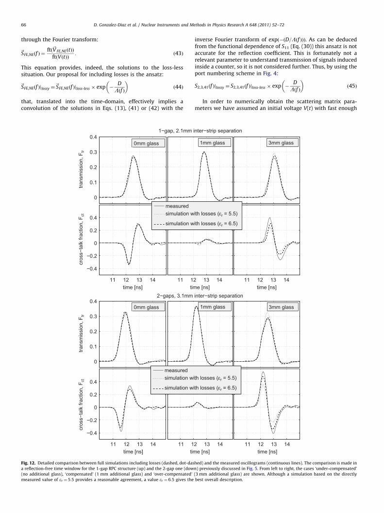
Fig. 12. Detailed comparison between full simulations including losses (dashed, dot-das
a reflection-free time window for the 1-gap RPC structure (up) and the 2-gap one (dow
(no additional glass), ‘compensated’ (1 mm additional glass) and ‘over-compensated’
measured value of er ¼ 5:5 provides a reasonable agreement, a value er ¼ 6:5 gives the
inverse Fourier transform of expð�ðD=Lðf ÞÞÞ. As can be deducedfrom the functional dependence of S11 (Eq. (30)) this ansatz is notaccurate for the reflection coefficient. This is fortunately not arelevant parameter to understand transmission of signals inducedinside a counter, so it is not considered further. Thus, by using theport numbering scheme in Fig. 4:
S2,3,41ðf Þjlossy ¼ S2,3,41ðf Þjloss-less � exp �D
Lðf Þ
� �ð45Þ
In order to numerically obtain the scattering matrix para-meters we have assumed an initial voltage V(t) with fast enough
11 12 13 14time [ns]
inter−strip separation
2 13 14e [ns]
ith losses (εr = 5.5)
ith losses (εr = 6.5)
1mm glass 3mm glass
11 12 13 14time [ns]
inter−strip separation
2 13 14e [ns]
ith losses (εr = 5.5)
ith losses (εr = 6.5)
1mm glass 3mm glass
hed) and the measured oscillograms (continuous lines). The comparison is made in
n) previously discussed in Fig. 5. From left to right, the cases ‘under-compensated’
(3 mm additional glass) are shown. Although a simulation based on the directly
best overall description.

D. Gonzalez-Diaz et al. / Nuclear Instruments and Methods in Physics Research A 648 (2011) 52–72 67
components in the range studied here. For simplicity, an exponentialsignal with 100 ps rise-time has been used. The procedure was:
(1)
Fig.cros
Obtain the solutions to the problem (Eqs. (41) and (42)).
(2) Make the Fourier transform, according to Eq. (43). (3) Apply the attenuation factor expð�ðD=Lðf ÞÞÞ obtained fromsimulations of the 1-strip transmission coefficient S21 as inFig. 9.
Fig. 11 shows the measurements of the scattering matrixcoefficients (left) and the corresponding simulations (right) forthe 2-gap/3-glass structure previously studied in Fig. 5 in a time-domain representation. The 1-strip transmission coefficient isshown as Sn
21(light gray) for reference. From up-down three casesare presented: under-compensated (no additional glass plate),compensated (one additional glass plate) and over-compensated(three additional glass plates). We note that the observedfrequency pattern of the compensated system is strikingly simple,as predicted in Fig. 8, allowing for an extended bandwidth (up to thelimit imposed by losses) and much reduced cross-talk patterns.
In order to reconcile the measurements in frequency domainin Fig. 11 with the ones in time-domain in Fig. 5 we haveconvoluted (under the factorization assumption (45)) the time-domain simulated waveforms in previous section with the inverseof the Fourier transform of expð�D=Lðf ÞÞ. The results are shownin Fig. 12 by zooming-in the direct signal (no reflections). Time-offsets have been adjusted in order to allow precise shape-comparisons, for which the simulations with er ¼ 5:5 (dotted)are used as reference, and both measurements (continuous) andsimulations with er ¼ 6:5 (dashed) are time-shifted to give thebest possible agreement. A detailed comparison of the mostrelevant observables is given in Fig. 13.
Despite the overall good agreement, simulations clearly favor avalue for er ¼ 6:5, contrary to the measurements in the frequencydomain, that favor er ¼ 5:5. Of course, by using er ¼ 6:5 thepropagation velocity, that is directly connected to the inter-peak
0.3
0.4
0.5
trans
mis
sion
(max
)
0 1 2 310−2
10−1
100
number of extra glass plates
cros
s−ta
lk (m
ax)
0
200
400
600
800
rise
time
[ps]
2−gaps, 3.1mm inter−strip
rise−time of the original signal
13. Comparison between measurements and simulations for the main characteris
s-talk fraction). The signal characteristics are very well described after including lo
distance in the frequency domain, (and is not included in Fig. 13)is not properly described in the time-domain representation, bysome 4%. This discrepancy is presumably stemming from plate toplate variations or slight material anisotropies, and it has to beunderstood as the systematic uncertainty present in these set ofmeasurements.
5. Electrostatic compensation in N-strip structures
A literal solution for N-strips, like the one given in Ref. [2] for2-strips, could be useful for counter optimization. Besides, it isimportant to understand to which extent the ideas introduced inthe previous section for the simple 2-strip case can be applied toan N-strip situation. Inspired by the work of Romeo and Santo-mauro [38], we propose to approximate C , C 0 by tri-diagonalmatrices. Translational invariance across the strips is alsoassumed, so that the electrostatic couplings of each strip are thesame with respect to its neighbors and ground.
For simplicity we study the 5-strip case that, we believe,contains the essential features of an N-strip RPC system. Thus,our input matrices have the form
X ¼
X0 �Xm 0 0 0
�Xm X0 �Xm 0 0
0 �Xm X0 �Xm 0
0 0 �Xm X0 �Xm
0 0 0 �Xm X0
0BBBBBB@
1CCCCCCA
ð46Þ
where X stands for either C or C 0. In Ref. [38] indeed, theassumption was made that L itself was tri-diagonal instead ofC 0. It seems to us that the latter approach provides generally ahigher accuracy for RPC structures and, besides, allows for slightlymore compact formulas; we will refer to this in the following asthe ‘short-range coupling’ approximation. The structures of theprevious section, for instance, show a value for the couplingcoefficient Cm=C0 � 1=10, while the (eventual) coupling to a
0 1 2 3number of extra glass plates
1−gap, 2.1mm inter−strip
measurementssimulation without losses (εr = 5.5)
simulation with losses (εr = 5.5)
simulation with losses (εr = 6.5)
tics of a typical signal (signal rise-time, maximum of the signal transmission and
sses, where the value er ¼ 6:5 for glass can be considered as an optimum choice.

D. Gonzalez-Diaz et al. / Nuclear Instruments and Methods in Physics Research A 648 (2011) 52–7268
second neighbor, in a translationally invariant structure, would beCm2=C0t1=100, so that assumption (46) is a priori justified.22
Beyond the 2-strip case, the ‘short-range coupling’ approximationimplies an artificially low coupling to ground for the first and thelast strips (at the sides of the structure). This is so because theC-matrices are defined such that the capacitance to ground ofstrip i satisfies the condition Cg,i ¼ C iiþ
PNj ¼ 1,ja i C ij, Cij are
defined negative, and those strips have one first-neighbor less.Signals produced at the side-strips of the structure will, therefore,show a deviation from the behavior predicted by this approxima-tion. Their overall influence in propagation will be increasinglysmall as the number of strips increases. The exact solution to thediagonalization problem (15) under the ‘short-range coupling’approximation (taking for commodity of operation the orthogonalrepresentation) has a simple form independently from the parti-cular values of the elements of the C-matrices:
M ¼ M�1¼
1
2
1ffiffi3p �1 2ffiffi
3p �1 1ffiffi
3p
�1 1 0 �1 12ffiffi3p 0 � 2ffiffi
3p 0 2ffiffi
3p
�1 �1 0 1 11ffiffi3p 1 2ffiffi
3p 1 1ffiffi
3p
0BBBBBBB@
1CCCCCCCA
ð47Þ
and the components of ~v are
~v ¼ c
ffiffiffiffiffiffiffiffiffiffiffiffiffiffiffiffiffiffiffiffiffiffiffiffiffiffiffiC00þ
ffiffiffi3p
Cm0
C0þffiffiffi3p
sCm,
ffiffiffiffiffiffiffiffiffiffiffiffiffiffiffiffiffiffiffiffiC00þCm0
C0þCm
s,
ffiffiffiffiffiffiffiC00
C0
s,
8<:
ffiffiffiffiffiffiffiffiffiffiffiffiffiffiffiffiffiffiffiC00�Cm0
C0�Cm
s,
ffiffiffiffiffiffiffiffiffiffiffiffiffiffiffiffiffiffiffiffiffiffiffiffiffiffiC00�
ffiffiffi3p
Cm0
C0�ffiffiffi3p
sCm
9=;:ð48Þ
The above-velocity spectra become fully degenerated when thevelocity dispersion, defined as Eq. (18)-right, equals zero and thus
Cm
C0¼
Cm0
C00ð49Þ
meaning that modal dispersion is exactly canceled, and all modestravel at a velocity given by v in Eq. (18)-left. Indeed, this crucialproperty can be easily generalized to an arbitrary number of strips.For this it is necessary to realize that the condition (49) implies,under the ‘short-range coupling’ approximation (Eq. (46)), that thematrices C and C 0 differ in a multiplicative constant. Thus, thematrix to be diagonalized in the basic problem of Eq. (15) becomes,after recalling Eq. (17), proportional to the unit-matrix, whose eigen-values are obviously identical. This result means, precisely, that anyinhomogeneous N-strip transmission line that is translationallyinvariant across the strips, does not consist of magnetic materialsand falls under the short-range approximation will show no modaldispersion when it is electrostatically compensated. Interestingly,this will hold even if the coupling to the 1st neighbor is high (low-coupling approximation not fulfilled).
Despite the simplicity of the solution to the diagonalizationproblem in Eqs. (47) and (48), a tractable literal solution requiresof further assumptions due to the need to obtain a simpleexpression for the transmission coefficient T in Eq. (13). Wepropose the ‘low-coupling’ assumption:
Cm
C0,Cm0
C00o1 ð50Þ
that is familiar from the 2-strip situation [2], where it has beendefined through the equivalent condition Zm=Zc o1. It is alsoassumed ‘moderate dispersion’, that means that Eq. (49) is alwaysapproximately satisfied. Under this latter assumption we keep thelowest order dispersive terms, that are the ones proportional to
22 Note that C0 ¼ CgþCm in the 2-strip case. In general, it is not easy to
strongly violate any of these two conditions for typical RPC designs. A remarkable
exception is Ref. [1], due the fact of w=h51.
the difference of the traveling modes. At last, we inject a signal I(t)at position y0 along the second strip and obtain the transmittedand cross-talk signals in the 3rd (1st neighbor) and 4th (2ndneighbor) strips, in order to avoid side effects.
The literal solutions for injection at an arbitrary position y0,omitting reflections, can be finally obtained
ItrðtÞCT
2
S1Iðt,y0ÞþS2Iðt,y0Þ
2þ
ZmR
ðZcþRÞ2
ffiffiffi3p
D1Iðt,y0ÞþD2Iðt,y0Þ
2ð51Þ
Ict,1ðtÞCZmR
ðZcþRÞ2S1Iðt,y0Þþ
T
2ffiffiffi3p D1Iðt,y0Þ ð52Þ
Ict,2ðtÞCðZmRÞ2
ðZcþRÞ31
Zc
S1Iðt,y0ÞþS2Iðt,y0Þ
2þ
T
2
S1Iðt,y0Þ�S2Iðt,y0Þ
2ð53Þ
with
S1ð2ÞIðt,y0Þ ¼1
2I t�
y0
v5ð4Þ
� �þ I t�
y0
v1ð2Þ
� �� �ð54Þ
D1ð2ÞIðt,y0Þ ¼1
2I t�
y0
v5ð4Þ
� ��I t�
y0
v1ð2Þ
� �� �: ð55Þ
The structure of the solutions in Eqs. (51)–(53) highlights theformal analogy with the literal solutions to the 2-strip problemgiven in Ref. [2]. When the system is compensated and reflectionsare neglected, transmission becomes independent from the signalshape, the propagation distance and the position and thus
Ftr ¼T
2ð56Þ
Fct,1 ¼R
ZcþR
� �Zm
Zcð57Þ
Fct,2 ¼R
ZcþR
� �Zm
Zc
� �2
¼ F2ct,1 ð58Þ
implying a flat time (and frequency) response.In order to illustrate the power of the electrostatic compensation
technique we have performed simulations for two realistic 5-stripRPCs, each strip being 2.5 cm-wide. One of the structures is a 2-gap/3-glass micro-strip structure (like in the previous sections), but theground plane has been also segmented and consists of five stripsidentical to the signal strips. The second structure is a strip-linestructure. Precisely, it is the same micro-strip structure but mirroredwith respect to the signal plane. The inter-strip separation is assmall as 1 mm in both cases. Compensation has been achieved inthe first case by adding 0.35 mm-thick glass over the signal plane(er ¼ 5:5), while in the second case two additional layers of Teflon(er ¼ 2:1), 0.48 mm-thick, have been added up and down withrespect to the signal plane (Fig. 14). A compilation of the mainelements of the capacitance matrices is given in Table 2.
Fig. 15 shows the results of the proposed optimization on5-strip structures, serving also as a comparison between the exactsolutions (left) and the literal solutions given in Eqs. (51)–(53)(right). The same signal used in the measurements of previoussection has been injected at the center of a 4 m-long counter, andreflections have been omitted. Compensation has been achievedin both micro-strip and strip-line configurations, although thecross-talk level stays higher in the micro-strip case than in thestrip-line one. This is because of the presence of two close-byground planes in the strip-line configuration, unlike the micro-strip, thus confining the mutual coupling field to a smallervolume in the former case and reducing the coupling coefficient(Table 2). Besides, the coupling to the second neighbor is almost

Fig. 14. Two electrostatically compensated 5-strip RPCs studied in this section.
Table 2Compilation of the main capacitive elements, in pF/m, for various 5-strip RPCs
under the following definitions C0 � C 33, Cm ��C 23, Cm2 ��C 13, and similarly for
the elements of matrix C0 .
Structure C0 Cm Cm2 C00 Cm0 Cm02
Micro-strip (uncomp.) 276.2 36.1 1.23 98.7 15.7 1.21
Micro-strip (comp.) 299.7 47.8 1.26 98.7 15.7 1.21
Strip-line (uncomp.) 499.8 49.6 0.0006 144.9 8.9 0.00035
Strip-line (comp.) 390.0 28.3 0.00036 131.4 9.5 0.00026−0.6−0.4−0.2
00.20.40.6
fract
ion
of s
igna
l
11 12 13 14
−0.1
0
0.1
0.2
0.3
time [ns]
fract
ion
of s
igna
l
11 12 13 14time [ns]
transmission Ftr
cross−talk 1st Fct, 1
cross−talk 2nd Fct, 2
micro−stripexact solution literal solution
−0.6−0.4−0.2
00.20.40.6
fract
ion
of s
igna
l
11 12 13 14
−0.1
0
0.1
0.2
0.3
time [ns]
fract
ion
of s
igna
l
11 12 13 14time [ns]
transmission Ftr
cross−talk 1st Fct, 1
cross−talk 2nd Fct, 2
strip−lineexact solution literal solution
un−compensated
un−compensated
compensated
compensated
Fig. 15. Up-set: simulations for transmission along 4 m-long 5-strip RPC in a micro-
strip configuration as described in text, with 2.5 cm-wide strips placed as close as
1 mm. Signal induction takes place at the center, y0 ¼ 2 m. The left column shows the
exact solution and the right one the literal solutions given in text. The upper row stands
for a non-compensated case and the lower one for a compensated one. The fraction of
transmitted signal (continuous), fraction of cross-talk to the first neighbor (dashed) and
fraction of cross-talk to the second neighbor (dot-dashed) are shown. Low-set: like the
upper set but for a 5-strip-line configuration as described in text, also with 2.5 cm
width and 1 mm inter-strip separation.
D. Gonzalez-Diaz et al. / Nuclear Instruments and Methods in Physics Research A 648 (2011) 52–72 69
nonexistent in this strip-line structure, making the ‘short-rangecoupling’ approximation virtually exact, unlike the micro-strip.Because of that, compensation is exactly achieved, and the cross-talk to the second neighbor is as small as Fct,2 ¼ F2
ct,1C0:052, fromEq. (58). Due to the higher coupling to the second neighbor, thissituation is not reached in the micro-strip configuration, showingFct,2 � Fct,1.
A convenient characterization of the full N-strip problem canbe indeed obtained by resorting to the ‘2-strip parameters’together with a parameter that characterizes the losses (tandn).We define two additional auxiliary parameters, the modaldispersion strength Y and the long-range coupling strength X as
Y¼Dv
v
��������pLe ð59Þ
X¼Cm2=Cm
Cm=C0¼
Cm2C0
C2m
: ð60Þ
The former represents the proportionality coefficient between thedispersive term of the cross-talk signal and the transmitted one inthe limit where dispersion is small [2]. A compilation of theparameters proposed for characterizing transmission in N-stripRPCs is given in Table 3.
At last, we want to analyze the ‘directional coupler’ limitpreviously introduced. As said, this limit is obtained for signalinjection at one of the ends of the structure in Eq. (13) after theequivalence of Eq. 22. We will focus on the far-end characteristics.Let us assume that the structure is already compensated: in thiscase, the equations are substantially simplified (the formula isgiven in Eq. (B.12)). Essentially, the matrix product over the modescollapses into a single vector current whose only non-zero elementis I(t) for the strip where injection is made. Since the signal isinjected at one end we have to add the first reflection. Thereflection coefficient is (1�T ) (and we assume in the followingthat the injection line is 2). Thus, as compared to Eqs. (56)–(58),there is an additional signal coupled to the neighbors at the

Table 3The ‘2-strip parameters’ together with the modal dispersion strength Y and the
long-range coupling strength X defined in text, proposed as an operational
characterization of transmission in (loss-less) N-strip RPCs. The last column gives
the dielectric losses.
Structure v=c Zc ðOÞ Zm=Zc Dv=v Y X tandn
Micro-strip (uncomp.) 0.598 20.2 0.15 �0.0142 1.78 0.26 0.0135
Micro-strip (comp.) 0.574 19.4 0.16 0.0002 0.02 0.16 0.0135
Strip-line (uncomp.) 0.538 12.4 0.08 0.0189 2.37 0.0001 0.0135
Strip-line (comp.) 0.580 14.7 0.07 0.0001 0.01 0.0002 0.0107
D. Gonzalez-Diaz et al. / Nuclear Instruments and Methods in Physics Research A 648 (2011) 52–7270
induction point, and this coupling goes with �T23 and �T24,correspondingly. Neglecting high order terms
Ftr ¼ 2T
2þ 1�Tð Þ
T
2
� �ð61Þ
Fct,1 ¼R
ZcþR
� �Zm
Zc�
R
ZcþR
� �Zm
ZcT
� 1
1þð1�TÞð62Þ
Fct,2 ¼R
ZcþR
� �Zm
Zc
� �2
�R
ZcþR
� �Zm
Zc
� �2
T
( )1
1þð1�TÞð63Þ
When the system is matched with a single resistor (Zc ¼ R) thenT¼1 and we obtain, within the approximations, Ftr C1, Fct,1C0,Fct,2C0, as for the directional coupler. Note that for signal injectionat any arbitrary position except at the ends, it is not possible toexactly cancel cross-talk. This is so because the process is driven byan ideal (infinite impedance) current source, unlike in a classicaldirectional coupler (where the source impedance is matched tothat of the line).
6. Discussion
The measurements performed in Sections 4 and 5 are equivalentwithin the limits of the precision of the corresponding apparatuses.This equivalence has been here presented through Figs. 11, 12 and13. Complementary, it is possible to compare the Fourier-trans-formed time-domain measurements in Section 4 with the measure-ments performed with the network analyzer in Section 5. This hasbeen done and shows naturally a good agreement, but with a muchlower precision, specially above 1.5 GHz, where the frequencycomponents of the pulser used (280 ps rise-time) are much sup-pressed, and sensitivity is lost. In particular, this approach does notallow to isolate neither the losses nor the deviations from a TEMdescription as precisely as it has been done with the networkanalyzer data. Besides, Fourier-transformed time-domain data hasa much lower frequency sampling as compared with the measure-ments from the network analyzer.
Despite we have found evidence of systematic variations of boththe glass loss-tangent tandjglass ¼ 0:2570:05 and its dielectric con-stant er ¼ 670:5, a very satisfactory description of several datataken in different conditions has been obtained. Additionally,‘electrostatic compensation’ has been experimentally demonstratedfor 1- and 2-gap structures allowing to obtain a factor �12reduction in cross-talk for a typical signal as measured with a� 2 GHz bandwidth system. Thus, as it seems, the frequency-dependence of the parameters, eventual anisotropies, as well asplate to plate variations and/or line non-uniformities, in general, donot represent an obvious limitation when trying to compensate RPCstructures. Moreover, an ‘a priori’ design seems possible, if tightmechanical tolerances at the 0.1 mm scale are observed.
Transmission along the compensated systems here developedwas limited only by the dielectric losses. As shown, however,losses depend little on the system geometry for wide structures,
so there is no much room for optimization. The most obvious (andmaybe only) way consists on reducing the glass thickness oradding an additional material with a small series capacitance andlow loss tangent (Teflon, for instance), that imply a reduction oftandn through the factor FG. If a proper selection of the glass isincluded, it seems likely that the bandwidth of a compensatedRPC based on float glass could be extended virtually to the limitimposed by the intrinsic signal rise-times (3 GHz) up to 2 m.
It must be noted that this is the first experimental verification ofthe existence of modal dispersion in RPC structures, besides theindirect results in Ref. [2]. According to our simulations, the band-stop region stemming from modal dispersion is centered around600 MHz for the structures previously studied in Ref. [21], far fromthe limit of the device used for those measurements (200 MHz).
There are classical ideas on cross-talk minimization that havebeen also studied prior to the elaboration of this work and will behere described generally. A final quantitative evaluation is muchsystem-dependent so only general arguments are given:
(1)
A ground plane (or a cage) close (or around) to the strip canarbitrarily reduce the coupling coefficient Zm=Zc , thus will alwaysreduce cross-talk for short strips, at the expense of a reducedimpedance. However, compensation is not guaranteed by thisprocedure, so low cross-talk and high transmission cannot beensured for long counters by just observing this principle.(2)
Shielding vias or the usage of additional materials with lowdielectric constants can reduce the coupling coefficient Zm=Zc .They take, however, a small portion of the available fieldlines, that propagate through the glass/gap structure anyhow.Modest improvements in transmission and cross-talk can benevertheless achieved.(3)
We have presented here single-ended signal measurementson single-ended architectures. So it is implicitly assumed thatall outer electrodes constitute the reference/return. On theother hand, differential signaling is known to give, in general,lower levels of cross-talk as compared to single-ended signal-ing, and a faster decrease with the inter-trace separation [39].This is natural for large distances between each differentialpair, since the coupling becomes then identical for both tracesof the same pair and cancels when the difference is taken.This is not, however, a typical situation for RPC structures andwe have found so far no evidence that this principle prevails.The description of a truly differential system requires manipulat-ing a large number of parameters (15�15 matrixes are needed forsimulating the structure of Fig. 14-down). A literal solution to thatproblem in the way presented here is out of the scope of this work.Simulations based on Eq. (10) can be, however, performed for thestructure of Fig. 14-down in three representative cases: (i) a puresingle-ended system (matrixes 5�5) terminated with R¼ 50 O asstudied in the main body of this document, (ii) a differential system(matrixes 15�15, signals injected at central and outer electrodes)read out differentially (Rdiff ¼ 100 O) and (iii) a differential systemread out in single-ended mode. In all three cases, the cross-talkpatterns shown in Fig. 15 do not differ by more than a 10%. This canbe interpreted as the fact that ‘electrostatic compensation’ is aproperty of the RPC structure, being the associated optimal transmis-sion characteristics little dependent from the way its readout is made.Nevertheless, this subject certainly deserves further investigations.
7. Conclusions
We say that a strip counter is ‘electrostatically compensated’when the coupling coefficient Zm=Zc CCm=C0 is the same in the filledand in the empty structure. Equivalently, the capacitive and inductive
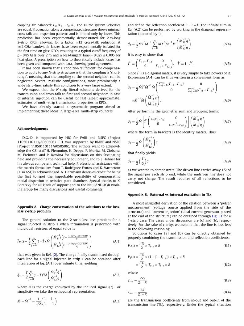
D. Gonzalez-Diaz et al. / Nuclear Instruments and Methods in Physics Research A 648 (2011) 52–72 71
coupling are balanced: Cm=C0 ¼ Lm=L0 and all the system velocitiesare equal. Propagation along a compensated structure shows minimalcross-talk and dispersion patterns and is limited only by losses. Thisprediction has been experimentally demonstrated for 2 m-long2-strip RPCs, allowing for a factor �12 cross-talk reduction atC2 GHz bandwidth. Losses have been experimentally isolated forthe first time on glass RPCs, resulting in a typical cutoff frequency offc¼0.85 GHz over 2 m and a loss-tangent tand¼ 0:02570:005 forfloat glass. A prescription on how to theoretically include losses hasbeen given and compared with data, showing good agreement.
It has been shown that a condition ‘sufficient’ for compensa-tion to apply to any N-strip structure is that the coupling is ‘short-range’, meaning that the coupling to the second neighbor can beneglected. Several realistic configurations, most prominently awide strip-line, satisfy this condition to a very large extent.
We expect that the N-strip literal solutions derived for thetransmission and cross-talk to first and second neighbors in caseof internal injection can be useful for fast (albeit approximate)estimates of multi-strip transmission properties in RPCs.
We have already started a systematic program aimed atimplementing these ideas in large-area multi-strip counters.
Acknowledgments
D.G.-D. is supported by HIC for FAIR and NSFC (Project11050110111/A050506), C.H. was supported by BMBF and NSFC(Project 11050110111/A050506). The authors want to acknowl-edge the GSI staff H. Flemming, H. Deppe, P. Moritz, M. Ciobanu,M. Freimuth and P. Kowina for discussions on this fascinatingfield and providing the necessary equipment, and to J. Hehner forhis always competent technical help. Professional assistance withthe matrix formalism from T. Rodrıguez Frutos and K. Vartortout(also GSI) is acknowledged. N. Herrmann deserves credit for beingthe first to spot the improbable possibility of compensatingmodal dispersion in resistive plate chambers. Special thanks to K.Boretzky for all kinds of support and to the NeuLAND-R3B work-ing group for many discussions and useful comments.
Appendix A. Charge conservation of the solutions to the loss-less 2-strip problem
The general solution to the 2-strip loss-less problem for asignal injected in strip 1 when termination is performed withindividual resistors of equal value is
~IT ðtÞ ¼T
2
X1j ¼ 0
ð1�T ÞjMM�1
11 I t� ð�1Þjy0þ2dj=2eDv1
�M�1
12 I t� ð�1Þjy0þ2dj=2eDv2
�0B@
1CA ðA:1Þ
that was given in Ref. [2]. The charge finally transmitted througheach line for a signal injected in strip 1 can be obtained afterintegration of Eq. (A.1) over infinite time, yielding
~qT ¼T
2
X1j ¼ 0
ð1�T ÞjMM�1
11 q
M�1
12 q
0@
1A ðA:2Þ
where q is the charge conveyed by the induced signal I(t). Forsimplicity we take the orthogonal representation:
M ¼ M�1¼
1ffiffiffi2p
1 1
1 �1
� �ðA:3Þ
and define the reflection coefficient G ¼ 1�T . The infinite sum inEq. (A.2) can be performed by working in the diagonal represen-tation (denoted by 0):
~qT ¼1
2MT
0M�1 X1
j ¼ 0
MG0jM�1
MM�1
11 q
M�1
12 q
0@
1A: ðA:4Þ
It is easy to show that
G0¼
G11�G12 0
0 G11þG12
!, T
0¼ 1�G
0: ðA:5Þ
Since G0
is a diagonal matrix, it is very simple to take powers of it.Expression (A.4) can be thus written in a convenient form as
~qT ¼1
2MT
0M�1
M
P1j ¼ 0ðG11�G12Þ
j 0
0P1
j ¼ 0ðG11þG12Þj
0@
1A
�M�1
MM�1
11 q
M�1
12 q
0@
1A: ðA:6Þ
After performing the geometric sum and grouping terms:
~qT ¼1
2M T
01
1�ðG11�G12Þ0
0 11�ðG11þG12Þ
0@
1A
24
35 M
�1
11 q
M�1
12 q
0@
1A ðA:7Þ
where the term in brackets is the identity matrix. Thus
~qT ¼1
2M
M�1
11
M�1
12
0@
1Aq ðA:8Þ
that finally yields
~qT ¼1
2
1
0
� �q ðA:9Þ
as we wanted to demonstrate. The driven line carries away 1/2 ofthe signal per each strip end, while the undriven line does notcarry net charge. The result requires of all reflections to beconsidered.
Appendix B. External vs internal excitation in TLs
A most insightful derivation of the relation between a ‘pulsermeasurement’ (voltage source applied from the side of thestructure) and ‘current injection’ (ideal current generator placedat the end of the structure) can be obtained through Fig. B1 for a1-strip case. The cases under discussion are (c) and (b), respec-tively. For the sake of clarity, we assume that the line is loss-lessin the following reasoning.
Solutions to cases (a) and (b) can be directly obtained byproperly combining the transmission and reflection coefficients:
VaðtÞ ¼IðtÞ
2� Ti�o � R ðB:1Þ
VbðtÞ ¼IðtÞ
2� ð1þð1�Ti�oÞÞ � Ti�o � R
¼IðtÞ
2� To�i � Ti�o � R ðB:2Þ
where
Ti�o ¼2Zc
ZcþRðB:3Þ
To�i ¼2R
ZcþRðB:4Þ
are the transmission coefficients from in-out and out-in of thetransmission line (TL), respectively. Under the typical situation

Fig. B1. The three cases discussed for illustrating the equivalence between current
and voltage sources.
D. Gonzalez-Diaz et al. / Nuclear Instruments and Methods in Physics Research A 648 (2011) 52–7272
Zc oR, it is verified that Ti�oo1 and To�i41. According to thedefinitions in text:
Ftr,aðtÞ ¼1
2
IðtÞ
max½IðtÞ�� Ti�o � R ðB:5Þ
Ftr,bðtÞ ¼1
2
IðtÞ
max½IðtÞ�� To�i � Ti�o � R: ðB:6Þ
Perhaps counter-intuitively, transmission at the center of anunmatched loss-less strip (with Zc oR) will be always smallerthan at its ends, when looking at the signal collected at theopposite end. The factor between the two situations is To�i andarises from the constructive interference between the direct andreflected waves.
The solution in situation (c) is also easy to find, being
Vc,oðtÞ ¼Vc,iðtÞ
2R� To�i � Ti�o � R: ðB:7Þ
The voltage measured in the absence of TL or with it beingadapted is thus
VðtÞ ¼ Vc,iðtÞ=2 ðB:8Þ
as for a perfect voltage divider. The correspondence betweensituations (b) and (c) (Eqs. (B.2) and (B.7)) can be obtainedthrough the equivalence:
IðtÞ �Vc,iðtÞ
RðB:9Þ
or
IðtÞ � 2VðtÞ
RðB:10Þ
that is Eq. (22) in text. It provides the equivalence between thecurrent induced at one end of a TL via an ‘ideal’ current generator,I(t), and a ‘real’ voltage source Vc,i ¼ 2VðtÞ of output resistance R.Thus, the solutions to the former case (Eq. (13)) can be directlyapplied to the latter, after making the equivalence (B.10). Thisallows to employ Eq. (41) given in text.
A rigorous proof of the very useful equivalences (B.9) and(B.10) for the general N-strip case can be obtained by directcomparison of Eq. (10) for injection at the end y0 ¼D with thesolutions derived in Ref. [3] for pulser measurements, in thehomogeneous case. In such situation only one mode survives andEq. (10) collapses into
~V T ðtÞ ¼1þG0
2
X1j ¼ 0
ðGDG0Þj Zc
~I t�Dþ2jD
v
� ��
þGDZc~I t�
2ðjþ1ÞD�D
v
� �ðB:11Þ
or
~V T ðtÞ ¼1þG0
2
X1j ¼ 0
ðGDG0Þjð1þGDÞZc
~I t�Dþ2jD
v
� �: ðB:12Þ
Eq. (B.12) coincides with expression Eq. (9.21b) in Ref. [3] underequivalence (B.10), when the structure is driven from one end.
References
[1] A. Schuettauf, Nucl. Instr. and Meth. A 602 (2009) 679.[2] D. Gonzalez-Diaz, Nucl. Instr. and Meth. A, in press, doi:10.1016/j.nima.2010.
09.067.[3] C.R. Paul, Analysis of Multiconductor Transmission Lines, John Wiley & Sons,
2008.[4] J. de Urquijo, et al., Eur. Phys. J. D 51 (2009) 241.[5] P. Camarri, et al., Nucl. Instr. and Meth. A 414 (1998) 317.[6] P. Fonte, et al., Nucl. Instr. and Meth. A 48 (4) (2000) 201.[7] M. Ciobanu, et al., IEEE Trans. Nucl. Sci. NS-54 (4) (2007) 1201.[8] D. Belver, et al., IEEE Trans. Nucl. Sci. NS-57 (5) (2010) 2848.[9] A. Blanco, et al., IEEE Trans. Nucl. Sci. NS-48 (4) (2001) 1249.
[10] C. Lippmann, W. Riegler, Nucl. Instr. and Meth. A 517 (2004) 54.[11] A. Blanco, et al., Nucl. Instr. and Meth. A 485 (2002) 328.[12] M. Abbrescia, et al., Nucl. Instr. and Meth. A 593 (2008) 263.[13] I. Deppner, et al., Nucl. Instr. and Meth. A, in press, doi:10.1016/j.nima.2010.
09.165.[14] C. Caesar, et al., Nucl. Instr. and Meth. A, in press, doi:10.1016/j.nima.2010.09.
163.[15] E. Casarejos, et al., Nucl. Instr. and Meth. A, in press, doi:10.1016/j.nima.2010.
09.069.[16] W. Llope, Nucl. Instr. and Meth. A, in press, doi:10.1016/j.nima.2010.07.086.[17] A. Blanco, et al., Nucl. Instr. and Meth. A, in press, doi:10.1016/j.nima.2010.
08.068.[18] M. Kis, et al., Nucl. Instr. and Meth. A, in press, doi:10.1016/j.nima.2011.02.
076.[19] P. Steinhaeuser, et al., Nucl. Instr. and Meth. A 390 (1997) 86.[20] V. Ammosov, et al., Nucl. Instr. and Meth. A 456 (2000).[21] W. Riegler, et al., Nucl. Instr. and Meth. A 481 (2002) 130.[22] T. Heubrandtner, et al., Nucl. Instr. and Meth. A 489 (2002) 443.[23] W. Riegler, Nucl. Instr. and Meth. A 491 (2002) 258.[24] W. Riegler, Nucl. Instr. and Meth. A 535 (2004) 287.[25] A. Akindinov, et al., Il nuovo Cimento B 124 (2) (2009) 235.[26] S. Ramo, Proc. IRE 27 (1939) 584.[27] C. Wei, et al., IEEE Trans. Microwave Theory Tech. 32 (1984) 439.[28] H. Alvarez-Pol, et al., Nucl. Instr. and Meth. A 535 (2004) 277.[29] /http://web.awrcorp.com/Usa/Products/APLACS (accessed 06.04.11).[30] G.I. Zysman, A. Kent Johnson, IEEE Trans. Microwave Theory Tech. 17 (10)
(1969) 753.[31] D. Pozar, Microwave Engineering, second ed., John Wiley & Sons, 1998.[32] A. Feller, H.R. Kaupp, J.J. Digiacomo, Cross-talk and reflections in high-speed
digital systems, in: Proceedings of the Fall Joint Computer Conference, 1965.[33] /http://www.wolfram.com/products/mathematica/index.htmlS (accessed 06.
04.11).[34] C.R. Paul, IEEE Trans. Electron. Comput. 44 (3) (2002) 413.[35] /http://www.ansoft.com/products/em/maxwell/S (accessed 06.04.11).[36] V.D. Frechette, Non Crystalline Solids, Wiley, New York, 1960.[37] A.R. Djordjevic, T.K. Sarkar, IEEE Trans. Microwave Theory Tech. 35 (10)
(1987) 898.[38] F. Romeo, M. Santomauro, IEEE Trans. Microwave Theory Tech. 35 (2) (1987)
132.[39] F. Xiao, et al., IEICE Trans. Commun. E90-B (6) (2007) 1305.