31 December 2008

Signal Processing for Bit-Patterned Media (BPM) Channels

Sheida Nabavi & Vijayakumar Bhagavatula

2

DSSC Channels Research Strategy

Low SNR will be one of the main challenges for future high-density storage systems

LDPC codes Iterative soft decoders

Channel models and signal processing approaches must be adapted to the new recording paradigms

Bit-patterned media (BPM)Two-dimensional magnetic recording (TDMR)Heat-assisted magnetic recording (HAMR)Multi-level cell flash memory & MRAM

Optimization of channels algorithms for hardware power/area/performance tradeoffs

3 3

LDPC Codes: Contributions

FPGA platform for LDPC decoder achieved 10-12 BERDesign, evaluation and encoder/decoder architecture of hardware-friendly progressive edge growth (PEG) quasi-cyclic LDPC codesEvaluation of LDPC codes under realistic magnetic recording channel models (not just AWGN)Improved reverse concatenation of LDPC codes and RLL codes using bit-flipping & interleavingSemi-analytical method for error floor estimation by identifying trapping sets using FPGA platform; estimated error floors down to 10-13 frame error ratesInvestigation of the concatenation of LDPC codes and outer RS codes

4

Error-pattern Flipping Chase2-type Decoder

Reed-Solomon (RS) codes are still of much use and interestSoft-decoding methods (e.g., Koetter-Vardy algorithm) proposed for error correction beyond half the minimum distance, but their complexity too highSoowoong Lee proposed a new Error-pattern flipping Chase2-type decoder , with parameter p

Flip dominant error-patterns before RLL decoder instead of bit-flipping or symbol-flipping Repeat error-only decoding with 2p modified received sequences while flipping p most probable error-patterns

6 6

TDMR Concept (INSIC) 

20grains

40 channel bits from encoder

10 user bits 10 user bits

encode(¼-rate)

soft 2D decode

(shingled-) write

process

40 channel bitswith soft info.

(scanning)

establish timing & position of

bit-cells

hi-resln2D readprocess

can almost see grains but not grain-boundaries

A.

B.

C. D.

E.

F.

not all channel bits get written on grains

10 bits in 1 μin2

= 10 Terabits/in2

cornerwriter

TDMRToy example:

Use 2D image analysis methods to decode user bits from recovered channel bits & soft info., and grain statistics

READINGWRITING

Courtesy: Roger Wood

7

PLB IP Interface

Register Files

Write logic

Read logic

PowerPC405

DataBlockRAM

InstructionBlockRAM

RDG

RDG LDPCENC

Channel

SOVALDPCDecoder

Iteration Control

Analysis

LDPC Error Floor Estimation via FPGA Emulation (Yu Cai & Prof. Ken Mai)

PowerPC

SOVA_LDPCClock rate improved from 20Mhz to 100Mhz (5X)Two parallel SOVA_LDPC fit in one FPGA (2X)

Two PowerPC per FPGAFive FPGAs per boardHigh speed interconnect80GB on board DRAM

FPGA based SoC

Two parallel SOVA_LDPC per FPGA (2X speedup)Utilize all 5 FPGAs (5X speedup)50X speedup over previous FPGA implementation1000X speedup over workstation implementation

Future PlansResource UsageFPGA Floorplan

BEE2 Board

.5GB/s .

DRAM

XilinxVirtexII Pro 70

DRAM

XilinxVirtexII Pro 70

DRAM

XilinxVirtexII Pro 70

DRAM

XilinxVirtexII Pro 70

DRAM

XilinxVirtex II Pro 70

8

BPM Signal Processing: Outline

Motivation for BPMBPM 2D Pulse responseBER analysis of BPM Mitigating the effects of inter-track interferenceModeling the media noise

9

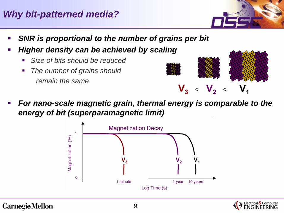
SNR is proportional to the number of grains per bitHigher density can be achieved by scaling

Size of bits should be reducedThe number of grains should

remain the same

For nano-scale magnetic grain, thermal energy is comparable to the energy of bit (superparamagnetic limit)

Why bit-patterned media?

10

Bits are stored in single domain magnetic islandsThe regions between the islands are nonmagnetic material Achieving densities over 1 Tb/in2

AdvantagesReducing transition and track edge noiseReducing or eliminating non-linear bit shiftSimplifying tracking

Bit-patterned media (BPM)

+ magnetization- magnetization

11

Inter-track interferenceBits or magnetic islands are very closeBesides ISI, there is ITI

Media noisemedia noise is caused by the fluctuations in the islands

LocationSizeThicknessMagnetizationShape

Write synchronizationFor more realistic channel model (modeling ITI and media noise) 2D pulse response needs to be used

Along track

Main Track

BPM challenges (signal processing)

...

...

.........

...

...... ......... ...

... .........

...

......... ...

...

...

...

12

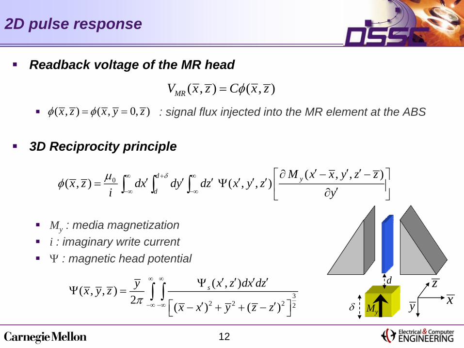
2D pulse response

Readback voltage of the MR head

: signal flux injected into the MR element at the ABS

3D Reciprocity principle

My : media magnetizationi : imaginary write currentΨ : magnetic head potential

( , ) ( , )MRV x z C x zφ=

( , ) ( , 0, )x z x y zφ φ= =

0 ( , , )( , ) ( , , )

d y

d

M x x y z zx z dx dy dz x y z

i yδμφ

∞ + ∞

−∞ −∞

′ ′ ′∂ − −⎡ ⎤′ ′ ′ ′ ′ ′= Ψ ⎢ ⎥′∂⎣ ⎦

∫ ∫ ∫

32 2 2 2

( , )( , , )2 ( ) ( )

s x z dx dzyx y zx x y z zπ

∞ ∞

−∞ −∞

′ ′ ′ ′ΨΨ =

′ ′⎡ ⎤− + + −⎣ ⎦∫ ∫

My

d

δ xy

z

13

Applying the head surface magnetic potential approximation from Wiesen et al.*

Example MR head surface magnetic potential

*K. Wiesen, and B. Cross, “GMR Head Side-Reading and Bit Aspect Ratio,” IEEE Trans. Magn., Vol. 39, No. 5, Sep. 2003

gW

tCro

ss-tr

ack

Along-track

12

12

2 2 4 2 22 1 2exp cos exp 1 exp cos1( , ) 1 arctan

2 2 41 2exp cos exp

s

z x z z xg g g g g

x zz x z

g g g

π π π π π

ππ π π

⎛ ⎞⎡ ⎤⎜ ⎟⎛ ⎞ ⎛ ⎞ ⎛ ⎞ ⎛ ⎞ ⎛ ⎞

− + − +⎢ ⎥⎜ ⎟ ⎜ ⎟ ⎜ ⎟ ⎜ ⎟ ⎜ ⎟⎜ ⎟⎝ ⎠ ⎝ ⎠ ⎝ ⎠ ⎝ ⎠ ⎝ ⎠⎛ ⎞ ⎣ ⎦⎜ ⎟Ψ = − ⎜ ⎟ ⎜ ⎟⎝ ⎠ ⎡ ⎤⎛ ⎞ ⎛ ⎞ ⎛ ⎞⎜ ⎟− +⎢ ⎥⎜ ⎟ ⎜ ⎟ ⎜ ⎟⎜ ⎟⎜ ⎟⎝ ⎠ ⎝ ⎠ ⎝ ⎠⎣ ⎦⎝ ⎠

MR head (W = 20 nm, t = 4 nm, g = 10 nm)

14

xyz

d

δa

t

g

W

Example 2D Pulse Response

Numerical integration to obtain the magnetic potential and pulse response

MR head t = 4 nm, W = 20 nm, gap = 10 nm

Magnetic islanda=11 nm, δ= 10 nm, d=10 nm

Along-track PW50=22.3 nm, Cross-track PW50=30.1 nm

15

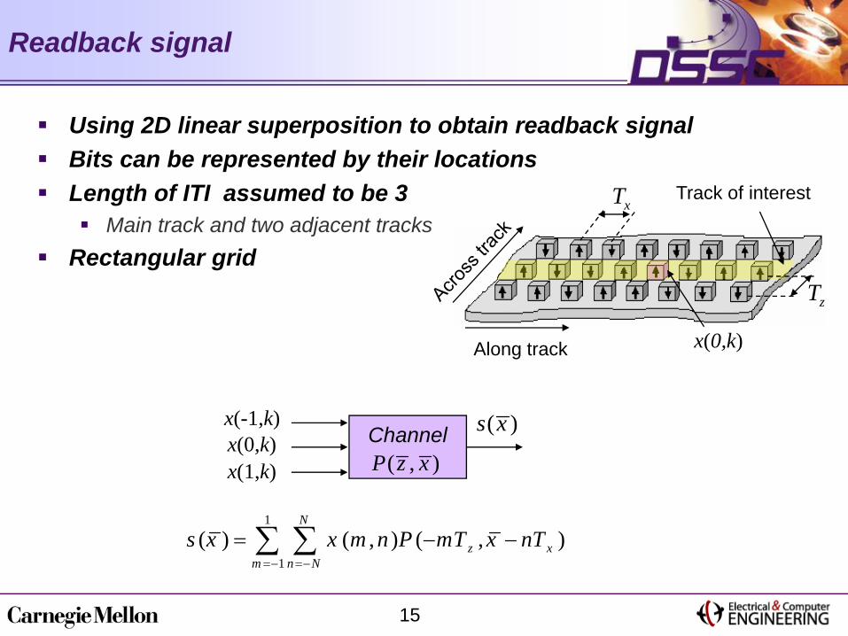
Readback signal

Using 2D linear superposition to obtain readback signalBits can be represented by their locations Length of ITI assumed to be 3

Main track and two adjacent tracksRectangular grid

1

1( ) ( , ) ( , )

N

z xm n N

s x x m n P mT x nT=− =−

= − −∑ ∑

Channelx(-1,k)x(0,k)x(1,k)

( )s x

( , )P z x

Along track x(0,k)

Track of interestxT

zT

16

Readback signal is sampled at the nominal bit period Tx

Discrete time readback signal

Equalizer outputAssuming symmetric channels

Discrete-time BPM read channel

H(m,n)=P(mTz, nTx)

1

1

( ) ( , ) ( , ) ( )N

m n N

r k x m n H m k n v k=− =−

= − − +∑ ∑

1

0

1

( )( )( )

h kh kh k−

← →⎡ ⎤⎢ ⎥= ← →⎢ ⎥⎢ ⎥← →⎣ ⎦

Hmatrix representation

Channelx(-1,k)x(0,k)x(1,k)

( )s x( , )P z x

r(k)+

v(k)

Equalizerf(k)

ViterbiDetector

z(k) ˆ(0, )x k

0 1

( ) ( ) ( )( ) ( ) (0, ) ( ) ( ) [ ( 1, ) (1, )] ( ) ( )

z k f k r kf k h k x k f k h k x k x k f k v k

= ∗= ∗ ∗ + ∗ ∗ − + + ∗

17

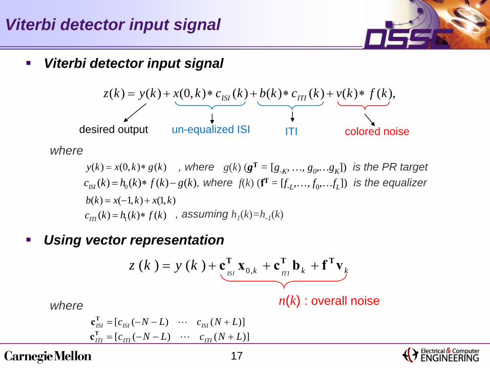
Viterbi detector input signal

Viterbi detector input signal

where, where g(k) (gT = [g-K, …, g0,…gK]) is the PR target

, where f(k) (fT = [f-L,…, f0,…fL]) is the equalizer

, assuming h1(k)=h-1(k)

Using vector representation

where

( ) (0, ) ( )y k x k g k= ∗

0( ) ( ) ( ) ( )ISIc k h k f k g k= ∗ −

( ) ( 1, ) (1, )b k x k x k= − +

1( ) ( ) ( )ITIc k h k f k= ∗

( ) ( ) (0, ) ( ) ( ) ( ) ( ) ( ),ISI ITIz k y k x k c k b k c k v k f k= + ∗ + ∗ + ∗

un-equalized ISI ITI colored noisedesired output

0,( ) ( )ISI ITIk k kz k y k= + + +T T Tc x c b f v

[ ( ) ( )]ISI ISI ISIc N L c N L= − − +Tc[ ( ) ( )]ITI ITI ITIc N L c N L= − − +Tc

n(k) : overall noise

18

For performance analysis of a partial response channel we need to first determine the error eventsFor the Viterbi detector, an error event ε is an erroneous estimate state sequence

Error event

Correct path Erroneous path

k1 k2

zk1 zk2-1

xk1-1xk1-2

-1 -1

-1 1

1 -1

1 1

-1 -1

-1 1

1 -1

1 1

-1 -1

-1 1

1 -1

1 1

-1 -1

-1 1

1 -1

1 1

19

Probability of an error event, ε

Probability of a particular error event ε for the Viterbi detector

wheremc is the path metric for the correct path

me the path metric for the erroneous path of a particular error event ε

wH(ε) : The number of input bit errors or the Hamming weight

For a specific error event ε

( )1Pr( ) Pr( )2

Hw

e cm mε

ε ⎛ ⎞≤ < ⎜ ⎟⎝ ⎠

2 2|| || ||c k kkm = − =z y n

2 2 2ˆ ˆ|| || || || ||e k k k k kkm = − = + − = +yz y y n y ε n

2 22 1Pr( ) Pr( ) Pr( )2e c k k y km m< = + < = < −T

y yn ε n ε n ε

20

pdf of

* : convolutionpdf of

vk : AWGN electronics noise

y kTε n

0,

0,

f ( ) f ( )

f ( )*f ( )y k ISI k ITI k f k

ISI k ITI k f k

= + +

= +

T T T T

T T T

ε n w x w b w v

w x w b w v

Gaussian(not Gaussian) ?

2(0, )k vv N σ→

f kTw v

22(0, )f v fN σ→Tw v w

The PDF of the overall noise and the output error sequence inner product

-1 1

1/2 1/2

x

f(x)

-2 0 2

1/21/41/4

b

f (b)

21

Distribution of ITI and un-equalized ISI

pdf ofAssuming uniform binary input data is a train of impulses

Monic constraint target (gT = [g-1, 1, g1]),Density of 2 Tbit/in2 , The minimum distance error event

0,ISI k ITI k+T Tw x w b0,f ( )ISI k ITI k+T Tw x w b

23

Most probable error events

Pr(ε) Pr(ε)++-+++0-+0++-++0+0-+0-0-+0+0+++-+--+-0++0-++-0-

4.037.138.988.038.08

10.2512.0812.0812.1312.0512.0511.1311.1311.18

1.66e-032.46e-051.48e-064.77e-066.33e-062.89e-071.13e-081.14e-081.51e-081.97e-082.02e-085.19e-085.19e-087.03e-08

+0+-++++-+-+0--+-+0++0++++0++0-0++-0+-+0-+-+-+0-+0+-++-+0++-0-+

11.1813.9613.3012.9812.9813.0313.0312.0314.2314.2514.2514.3114.3014.28

7.14e-081.07e-093.28e-093.34e-093.36e-094.33e-094.34e-098.50e-095.28e-105.29e-105.41e-107.36e-107.42e-107.72e-10

xεxε2

yε2

yε

Using computer search to obtain most probable error eventsMonic constraint target (gT = [g-1, 1, g1])Density of 2 Tbit/in2

σ2v= 0.01, The minimum distance error event, (dmin )2= 4.03

25

Conventional PR4 and EPR4 targets do not perform well

Vp=1σv : noise standard deviation

PR channels for BPM

e 10SNR 20 log ( / )p vV σ=

(db)

26

Analytical and simulation BER vs SNR

Monic constraint target gT = [g-1, 1, g1]

Density of 2 Tbit/in2

Tx and Tz 18 nmMR head

t = 4 nm, W = 20 nm, g = 10 nmMagnetic island

a=11 nm, δ= 10 nm, d=10 nm

0.021 0.213 0.0210.101 1 0.1010.021 0.213 0.021

⎡ ⎤⎢ ⎥= ⎢ ⎥⎢ ⎥⎣ ⎦

H

29

GPR equalizerTarget length : 3g = [g-1 1 g1]

Density of 2 Tbit/in2

Tx and Tz 18 nmMR head

t = 4 nm, W = 18 nm, g = 6 nmMagnetic island

a=11 nm, δ= 10 nm, d=10 nm

ITI significantly degrades the performance of the channel

Effect of Inter-track Interference (ITI)

0.038 0.294 0.0380.113 1 0.1130.038 0.294 0.038

⎡ ⎤⎢ ⎥= ⎢ ⎥⎢ ⎥⎣ ⎦

H

30

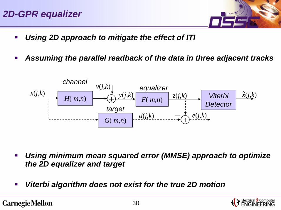
2D-GPR equalizer

Using 2D approach to mitigate the effect of ITI

Assuming the parallel readback of the data in three adjacent tracks

Using minimum mean squared error (MMSE) approach to optimize the 2D equalizer and target

Viterbi algorithm does not exist for the true 2D motion

G( m,n)

H( m,n) F( m,n)+v(j,k)

y(j,k) z(j,k)equalizer

target+

_ e(j,k)d(j,k)

x(j,k) x(j,k)Viterbi Detector

^

channel

31

j=0 is representing the main track

Mean square errorwhere

Vector representation for 2D GPR

, 0,0 ,

, 0,0 ,

, 0, ,

, 0, ,

T

M N M N

T

L L L L

T

k M k N k M k N

T

k L k L k L k L

f f f

g g g

y y y

x x x

− −

− −

+ − −

+ − −

⎡ ⎤= ⎣ ⎦

⎡ ⎤= ⎣ ⎦

⎡ ⎤= ⎣ ⎦

⎡ ⎤= ⎣ ⎦

f

g

y

x

… …

… …

… …

… …

( ) k ke k = T Tf y - g x

n(j,k)

G( m,n)

H( m,n) F( m,n)+y(j,k) z(0,k)=zk

equalizer

target +_e(k)

d(0,k)=dk

x(j,k)

{ }2( ) 2E e k = − +T T Tf Rf f Tg g Ag

{ } { } { }, ,k k k k k kE E E= = =T T TR y y T y x A x x

32

Minimizing the E{e(k)2} with considering the constraint

Lagrange functional to be minimized

where

2D GPR zero-ITI forcing equalizer (ZIFE)

2 2J = − + −T T T T Tf Rf f Tg g Ag λ (E g - c)

[ ]1 0 0 0 0 0 0 T=c

T T -1 -1 -1

T -1 -1

-1

λ = (E (A - T R T) E) cg = (A - T R T) Eλf = R Tg

Taking derivative respect to f, g and λ

0, 1 0,1

0 0 01

0 0 0g g−

⎡ ⎤⎢ ⎥= ⎢ ⎥⎢ ⎥⎣ ⎦

G or 0, 1 0,10 0 0 1 0 0 0T

g g−⎡ ⎤= ⎣ ⎦g

0 0 0 0 1 0 0 0 01 0 0 0 0 0 0 0 00 1 0 0 0 0 0 0 00 0 1 0 0 0 0 0 00 0 0 0 0 0 1 0 00 0 0 0 0 0 0 1 00 0 0 0 0 0 0 0 1

⎡ ⎤⎢ ⎥⎢ ⎥⎢ ⎥⎢ ⎥= ⎢ ⎥⎢ ⎥⎢ ⎥⎢ ⎥⎢ ⎥⎣ ⎦

TE

33

Results of 2D GPR ZIFE

2D GPR ZIFE3×3 targetObtained for σv

2=0.01

1D GPR (multi-track)Obtained for σv

2=0.01

2D GPR ZIFE improves the BER

0 0 00.132 1 0.130

0 0 0

⎡ ⎤⎢ ⎥= ⎢ ⎥⎢ ⎥⎣ ⎦

G

[ ]0.076 1 0.077 T=g

34

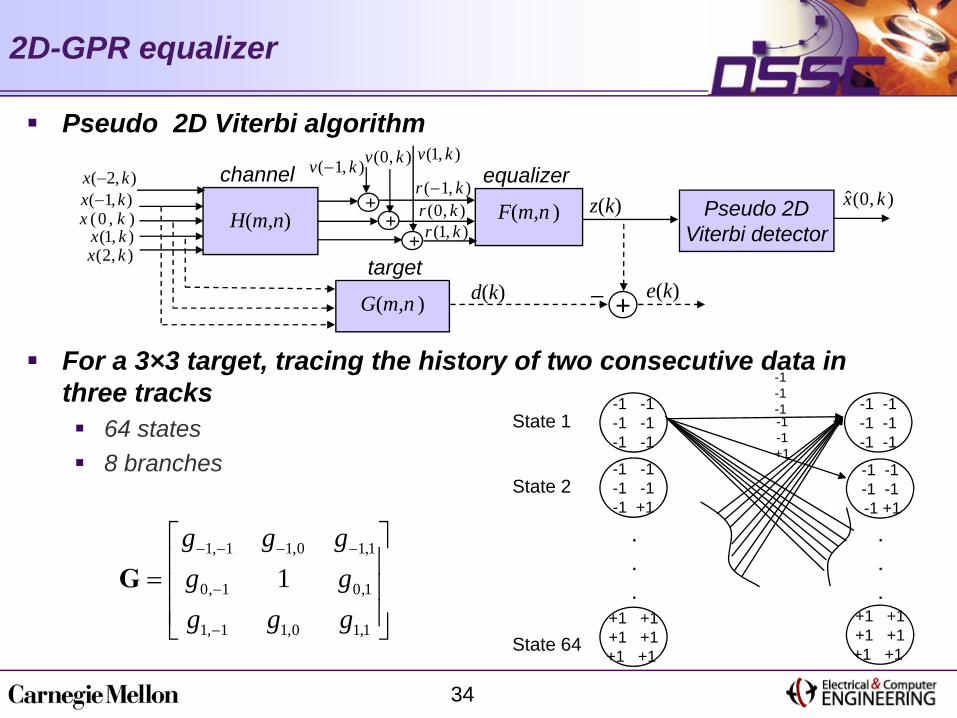
2D-GPR equalizer

Pseudo 2D Viterbi algorithm

For a 3×3 target, tracing the history of two consecutive data in three tracks

64 states 8 branches

1, 1 1,0 1,1

0, 1 0,1

1, 1 1,0 1,1

1g g gg gg g g

− − − −

−

−

⎡ ⎤⎢ ⎥= ⎢ ⎥⎢ ⎥⎣ ⎦

G

-1 -1-1 -1-1 -1

.

.

.+1 +1+1 +1+1 +1

-1 -1-1 -1-1 -1

-1 -1-1 -1-1 +1

.

.

.

-1 -1-1 -1-1 +1

+1 +1+1 +1+1 +1

-1-1 -1-1-1 +1

State 1

State 2

State 64

G(m,n )

H(m,n) F(m,n )+ z(k)equalizer

target

+_ e(k)d(k)

Pseudo 2D Viterbi detector

channelˆ(0, )x k

++

( 1, )x k−( 2, )x k−

(0 , )x k(1, )x k(2, )x k

( 1, )v k− (0, )v k (1, )v k

(0, )r k( 1, )r k−

(1, )r k

35

2D GPR equalizers

2D GPR targetObtained for σv

2=0.01

0.056 0.310 0.0770.183 1 0.1800.051 0.315 0.068

⎡ ⎤⎢ ⎥= ⎢ ⎥⎢ ⎥⎣ ⎦

G

37

Modified Viterbi algorithm (VA)

The locations of bits (islands) are fixedOne track is readAssuming symetric channel

Along track x0,k Main Track

1

0

1

( )( )( )

h kh kh k

← →⎡ ⎤⎢ ⎥= ← →⎢ ⎥⎢ ⎥← →⎣ ⎦

H

0 1

( ) ( ) ( )( ) ( ) (0, ) ( ) ( ) ( ( 1, ) (1, )) ( ) ( )

z k f k r kf k h k x k f k h k x k x k f k v k

= ∗= ∗ ∗ + ∗ ∗ − + + ∗

r(k)ChannelH(m,n)

Equalizerf(k)

ViterbiDetector+

v(k)z(k)( 1, )x k−

(0, )x k(1, )x k

ˆ(0, )x k

38

Considering ITI in VA

ITI is mainly due to directly adjacent bits i.e. x-1,k , x1,k

Assuming no track mis-registration Desired equalizer output

Where

( ) (0, ) [ (1, ) ( 1, )] ( )kd g k x k x k x k n kα≅ ∗ + + − +

0( ) ( ) ( )g k h k f k= ∗

( ) ( ) ( )n k v k f k= ∗

( , ) {1, 1} [ (1, ) ( 1, )] { 2,0,2}x j k x k x k∈ − ⇒ + − ∈ −

1 0( ) ( )

kh k f kα

=∗

39

Modified VA trellis

Trellis with ITI

( ) (0, ) 2 ( )( ) (0, ) ( )( ) (0, ) 2 ( )

k

g k x k n kd g k x k n k

g k x k n k

α

α

∗ + +⎧⎪= ∗ +⎨⎪ ∗ − +⎩

trellis

40

Results of the modified VA

Target : g = [0.1 1 0.1]α = 0.2

Modified VA improves the performance of the channel

41

Modeling the Media Noise

Considering location fluctuations and size fluctuations

.........

...

......... ...

...

...

...

......... ......

a...

TxTz ......

...

...

...... ...

1

1( ) ( , ) ( , ( ) , ) ( )

m n N

z m x n mnm n N

r k x m n P mT T k n T T a a v k= =

=− =−

= − + Δ − + Δ + Δ +∑ ∑

Channel S(x)x(-1,k)x(0,k)x(1,k)

+ r(k)v(k)

-

( , )P z x

42

Obtaining an analytical 2D pulse response

Along-track pulse response can be considered as subtraction of two transitionsFor a<<PW50 derivative of transition pulses can be interpreted as pulse responses

2D Gaussian pulseUsing erf(x) as a transition response

2D Lorentzian pulseUsing arctan(x) as a transition response

Wx : along- track PW50 Wz : cross-track PW50

a

a/2

2 2

2 2

1( , ) exp{ ( )}2 x z

x zP x z Aσ σ

= − +along-track 50

2.3548xPWσ =

cross-track 502.3548z

PWσ =

2 2( , )

1/ 2 / 2x z

AP x zx z

W W

=⎛ ⎞ ⎛ ⎞

+ +⎜ ⎟ ⎜ ⎟⎝ ⎠⎝ ⎠

43

Comparison of the 2D Gaussian and numerical pulses

Channel density 2Tbit/inch2

GPR equalizerTarget: [g-1 1 g1]

along-track PW50

Cross-track PW50

2D Gaussian pulse is a good candidate to model the BPM pulse response

44

Modeling media noise using analytical pulse response

Location fluctuations Randomness at the sampling points of the 2D Gaussian pulse,

Size fluctuations Amplitude, along-track PW50 and cross-track PW50 fluctuations

where

1Wx aaΔ ≅ Δ

2Wz aaΔ ≅ Δ

3A aaΔ ≅ Δ

2 21( , ) ( )exp ,2 ( ) ( )

x zA

x Wx z Wz

x zP x z Ac W c W

⎧ ⎫⎡ ⎤⎛ ⎞ ⎛ ⎞+Δ +Δ⎪ ⎪⎢ ⎥= +Δ − +⎨ ⎬⎜ ⎟ ⎜ ⎟+Δ +Δ⎢ ⎥⎝ ⎠ ⎝ ⎠⎪ ⎪⎣ ⎦⎩ ⎭2.3548c =

45

Extracting size and location statistics, using image processing techniquesUsing an image of BPM nano-mask

Media noise characteristics

Courtesy of Chip Hogg and professor Sara Majetich

46

Location and size fluctuations

Location and size fluctuations can be modeled by Gaussian distributions

Along-track size fluctuationsAlong-track location fluctuation

47

Correlation coefficients

Location fluctuations are highly correlated

Size fluctuations are less correlated

Along-track location fluctuations

Along-track Size fluctuations

48

Modeling correlated noise

Passing white noise through a digital filterNoise auto-correlation function modeled by a decaying exponential

f(k)n(k) v(k)

R n(k

)

R v(k

)

( ) kvR k a=( ) ( )nR k kδ=

D

+

a

n(k) v(k)b

f(k)

2( ) ( 1) ( 1 ) ( )v k av k a n k= − + −

white noise colored noise

, |a|<1

49

Decaying exponential auto-correlation function is a good model for correlated media noise

Modeling correlated noise (cont’d)

Along-track location fluctuations, a=0.9

Along-track Size fluctuations, a=-0.15

50

Matched-pulse PR channelsMinimizing noise amplification of the equalizers

GPR channelsNoise whitening equalizers

NPML channelsNoise predicting detectorsPredictor filter is embedded in the VA

Read channel for BPM with media noise

v(k)r(k) PR

EqualizerNPML detector

z(k)

Predictor

y(k)

-+ +

ChannelH(m,n)

( 1, )x k−

(0, )x k(1, )x k

ˆ (0 , )x k

v(k)r(k) PR

EqualizerViterbi detector

y(k)+

ChannelH(m,n)

( 1, )x k−

(0, )x k(1, )x k

ˆ (0 , )x k

Media noise

Media noise

51

Channel density 2Tbit/inch2

PR equalizerg=[0.1 1 0.1]

GPR equalizerg=[g-1 1 g1]Obtained for σ 2=0.05and 6% fluctuations

NPML detectorg=[0.1 1 0.1]

Gaussian fluctuations

Highly correlated normalized location and size fluctuations

α =0.95

Error performance of the PBM channels with media noise

solid lines: no media noise, dashed lines: 8% size and location fluctuations and doted lines: 8%

normalized correlated size and location fluctuations.

21β α= −

52

Summary

2D pulse response of BPM obtained using the 3D reciprocity principleThe ITI has the dominant impact on the error performance of the BPM channels and taking ITI into account is important for BPM channelsThe 2D GPR equalizers and the modified VA improve the BER performance of the BPM channelsMedia noise is correlated and can be modeled by a Gaussian random process2D Gaussian pulse can be used for the BPM 2D pulse responseNPML channels improve the BER performance of the BPM channels in the presence of the correlated media noise