signal processing methods for the automatic transcription
TRANSCRIPT

Tampere University of TechnologyPublications 460
Anssi Klapuri
Signal Processing Methods for the AutomaticTranscription of Music
Thesis for the degree of Doctor of Technology to be presented withdue permission for public examination and criticism in Auditorium S1,at Tampere University of Technology, on the 17th of March 2004,at 12 o clock noon.
Tampere 2004
ISBN 952-15-1147-8ISSN 1459-2045

Copyright © 2004 Anssi P. Klapuri.
All rights reserved. No part of this work may be reproduced, stored in a retrieval system, or transmitted, in anyform or by any means, electronic, mechanical, photocopying, recording or otherwise, without prior permissionfrom the author.
http://www.cs.tut.fi/~klap/

Abstract
Signal processing methods for the automatic transcription of music are developed in this the-sis. Music transcription is here understood as the process of analyzing a music signal so as towrite down the parameters of the sounds that occur in it. The applied notation can be the tradi-tional musical notation or any symbolic representation which gives sufficient information forperforming the piece using the available musical instruments. Recovering the musical notationautomatically for a given acoustic signal allows musicians to reproduce and modify the origi-nal performance. Another principal application is structured audio coding: a MIDI-like repre-sentation is extremely compact yet retains the identifiability and characteristics of a piece ofmusic to an important degree.
The scope of this thesis is in the automatic transcription of the harmonic and melodic parts ofreal-world music signals. Detecting or labeling the sounds of percussive instruments (drums) isnot attempted, although the presence of these is allowed in the target signals. Algorithms areproposed that address two distinct subproblems of music transcription. The main part of thethesis is dedicated to multiple fundamental frequency (F0) estimation, that is, estimation of theF0s of several concurrent musical sounds. The other subproblem addressed is musical meterestimation. This has to do with rhythmic aspects of music and refers to the estimation of theregular pattern of strong and weak beats in a piece of music.
For multiple-F0 estimation, two different algorithms are proposed. Both methods are based onan iterative approach, where the F0 of the most prominent sound is estimated, the sound is can-celled from the mixture, and the process is repeated for the residual. The first method is derivedin a pragmatic manner and is based on the acoustic properties of musical sound mixtures. Forthe estimation stage, an algorithm is proposed which utilizes the frequency relationships ofsimultaneous spectral components, without assuming ideal harmonicity. For the cancellingstage, a new processing principle, spectral smoothness, is proposed as an efficient new mecha-nism for separating the detected sounds from the mixture signal.
The other method is derived from known properties of the human auditory system. More spe-cifically, it is assumed that the peripheral parts of hearing can be modelled by a bank of band-pass filters, followed by half-wave rectification and compression of the subband signals. It isshown that this basic structure allows the combined use of time-domain periodicity and fre-quency-domain periodicity for F0 extraction. In the derived algorithm, the higher-order (unre-solved) harmonic partials of a sound are processed collectively, without the need to detect orestimate individual partials. This has the consequence that the method works reasonably accu-rately for short analysis frames. Computational efficiency of the method is based on calculat-ing a frequency-domain approximation of the summary autocorrelation function, aphysiologically-motivated representation of sound.
Both of the proposed multiple-F0 estimation methods operate within a single time frame andarrive at approximately the same error rates. However, the auditorily-motivated method issuperior in short analysis frames. On the other hand, the pragmatically-oriented method is“complete” in the sense that it includes mechanisms for suppressing additive noise (drums) andfor estimating the number of concurrent sounds in the analyzed signal. In musical interval andchord identification tasks, both algorithms outperformed the average of ten trained musicians.
i
For musical meter estimation, a method is proposed which performs meter analysis jointly atthree different time scales: at the temporally atomic tatum pulse level, at the tactus pulse levelwhich corresponds to the tempo of a piece, and at the musical measure level. Acoustic signalsfrom arbitrary musical genres are considered. For the initial time-frequency analysis, a newtechnique is proposed which measures the degree of musical accent as a function of time atfour different frequency ranges. This is followed by a bank of comb filter resonators which per-form feature extraction for estimating the periods and phases of the three pulses. The featuresare processed by a probabilistic model which represents primitive musical knowledge and per-forms joint estimation of the tatum, tactus, and measure pulses. The model takes into accountthe temporal dependencies between successive estimates and enables both causal and non-causal estimation. In simulations, the method worked robustly for different types of music andimproved over two state-of-the-art reference methods. Also, the problem of detecting thebeginnings of discrete sound events in acoustic signals, onset detection,is separately discussed.
Keywords—Acoustic signal analysis, music transcription, fundamental frequency estimation,musical meter estimation, sound onset detection.
ii

Preface
This work has been carried out during 1998–2004 at the Institute of Signal Processing, Tam-pere University of Technology, Finland.
I wish to express my gratitude to Professor Jaakko Astola for making it possible for me startworking on the transcription problem, for his help and advice during this work, and for hiscontribution in bringing expertise and motivated people to our lab from all around the world.
I am grateful to Jari Yli-Hietanen for his invaluable encouragement and support during the firstcouple of years of this work. Without him this thesis would probably not exist. I would like tothank all members, past and present, of the Audio Research Group for their part in making amotivating and enjoyable working community. Especially, I wish to thank Konsta Koppinen,Riitta Niemistö, Tuomas Virtanen, Antti Eronen, Vesa Peltonen, Jouni Paulus, MattiRyynänen, Antti Rosti, Jarno Seppänen, and Timo Viitaniemi, whose friendship and goodhumour has made designing algorithms fun.
I wish to thank the staff of the Acoustic Laboratory of Helsinki University of Technology fortheir special help. Especially, I wish to thank Matti Karjalainen and Vesa Välimäki for settingan example to me both as researchers and as persons.
The financial support of the Tampere Graduate School in Information Science and Engineering(TISE), the Foundation of Emil Aaltonen, Tekniikan edistämissäätiö, and the Nokia Founda-tion is gratefully acknowledged.
I wish to thank my parents Leena and Tapani Klapuri for their encouragement on my paththrough the education system and my brother Harri for his advice in research work.
My warmest thanks go to my dear wife Mirva for her support, love, and understanding duringthe intensive stages of putting this work together.
I can never express enough gratitude to my Lord and Saviour, Jesus Christ, for being the foun-dation of my life in all situations. I believe that God has created us in his image and put into usa similar desire to create things – for example transcription systems in this context. However,looking at the nature, its elegance in the best sense that a mathematician uses the word, I havebecome more and more aware that Father is quite many orders of magnitude ahead in engineer-ing, too.
God is faithfull, through whom you were called into fellowship with his son, Jesus Christ our Lord. –1.COR. 1:9
Tampere, March 2004
Anssi Klapuri
iii

iv

Contents
Abstract. . . . . . . . . . . . . . . . . . . . . . . . . . . . . . . . . . . . . . . . . . . . . . . . . . . . . . . . . . . . . . . . . . iPreface. . . . . . . . . . . . . . . . . . . . . . . . . . . . . . . . . . . . . . . . . . . . . . . . . . . . . . . . . . . . . . . . . . . iiiContents . . . . . . . . . . . . . . . . . . . . . . . . . . . . . . . . . . . . . . . . . . . . . . . . . . . . . . . . . . . . . . . . . vList of publications. . . . . . . . . . . . . . . . . . . . . . . . . . . . . . . . . . . . . . . . . . . . . . . . . . . . . . . . . viiAbbreviations . . . . . . . . . . . . . . . . . . . . . . . . . . . . . . . . . . . . . . . . . . . . . . . . . . . . . . . . . . . . . ix1 Introduction . . . . . . . . . . . . . . . . . . . . . . . . . . . . . . . . . . . . . . . . . . . . . . . . . . . . . . . . . . . . 1
1.1 Terminology . . . . . . . . . . . . . . . . . . . . . . . . . . . . . . . . . . . . . . . . . . . . . . . . . . . . . . . . 31.2 Decomposition of the music transcription problem . . . . . . . . . . . . . . . . . . . . . . . . . . 3
Modularity of music processing in the human brain . . . . . . . . . . . . . . . . . . . . . . . 3Role of internal models . . . . . . . . . . . . . . . . . . . . . . . . . . . . . . . . . . . . . . . . . . . . . 5Mid-level data representations . . . . . . . . . . . . . . . . . . . . . . . . . . . . . . . . . . . . . . . . 6How do humans transcribe music? . . . . . . . . . . . . . . . . . . . . . . . . . . . . . . . . . . . . 7
1.3 Scope and purpose of the thesis . . . . . . . . . . . . . . . . . . . . . . . . . . . . . . . . . . . . . . . . . 7Relation to auditory modeling . . . . . . . . . . . . . . . . . . . . . . . . . . . . . . . . . . . . . . . . 8
1.4 Main results of the thesis . . . . . . . . . . . . . . . . . . . . . . . . . . . . . . . . . . . . . . . . . . . . . . 9Multiple-F0 estimation system I . . . . . . . . . . . . . . . . . . . . . . . . . . . . . . . . . . . . . . 9Multiple-F0 estimation system II . . . . . . . . . . . . . . . . . . . . . . . . . . . . . . . . . . . . . . 10Musical meter estimation and sound onset detection . . . . . . . . . . . . . . . . . . . . . . 11
1.5 Outline of the thesis . . . . . . . . . . . . . . . . . . . . . . . . . . . . . . . . . . . . . . . . . . . . . . . . . . 112 Musical meter estimation . . . . . . . . . . . . . . . . . . . . . . . . . . . . . . . . . . . . . . . . . . . . . . . . . 13
2.1 Previous work . . . . . . . . . . . . . . . . . . . . . . . . . . . . . . . . . . . . . . . . . . . . . . . . . . . . . . . 14Methods designed primarily for symbolic input (MIDI) . . . . . . . . . . . . . . . . . . . . 14Methods designed for acoustic input . . . . . . . . . . . . . . . . . . . . . . . . . . . . . . . . . . . 16Summary . . . . . . . . . . . . . . . . . . . . . . . . . . . . . . . . . . . . . . . . . . . . . . . . . . . . . . . . 17
2.2 Method proposed in Publication [P6] . . . . . . . . . . . . . . . . . . . . . . . . . . . . . . . . . . . . 172.3 Results and criticism . . . . . . . . . . . . . . . . . . . . . . . . . . . . . . . . . . . . . . . . . . . . . . . . . 19
3 Approaches to single-F0 Estimation . . . . . . . . . . . . . . . . . . . . . . . . . . . . . . . . . . . . . . . . 213.1 Harmonic sounds . . . . . . . . . . . . . . . . . . . . . . . . . . . . . . . . . . . . . . . . . . . . . . . . . . . . 213.2 Taxonomy of F0 estimation methods . . . . . . . . . . . . . . . . . . . . . . . . . . . . . . . . . . . . . 233.3 Spectral-location type F0 estimators . . . . . . . . . . . . . . . . . . . . . . . . . . . . . . . . . . . . . 24
Time-domain periodicity analysis methods . . . . . . . . . . . . . . . . . . . . . . . . . . . . . . 24Harmonic pattern matching in frequency domain . . . . . . . . . . . . . . . . . . . . . . . . . 25A shortcoming of spectral-location type F0 estimators . . . . . . . . . . . . . . . . . . . . . 26
3.4 Spectral-interval type F0 estimators . . . . . . . . . . . . . . . . . . . . . . . . . . . . . . . . . . . . . . 263.5 “Unitary model” of pitch perception . . . . . . . . . . . . . . . . . . . . . . . . . . . . . . . . . . . . . 27
Periodicity of the time-domain amplitude envelope . . . . . . . . . . . . . . . . . . . . . . . 27Unitary model of pitch perception . . . . . . . . . . . . . . . . . . . . . . . . . . . . . . . . . . . . . 28Attractive properties of the unitary model . . . . . . . . . . . . . . . . . . . . . . . . . . . . . . . 29
4 Auditory-model based multiple-F0 estimator . . . . . . . . . . . . . . . . . . . . . . . . . . . . . . . . 314.1 Analysis of the unitary pitch model in frequency domain . . . . . . . . . . . . . . . . . . . . . 31
Auditory filters (Step 1 of the unitary model) . . . . . . . . . . . . . . . . . . . . . . . . . . . . 32Flatted exponential filters . . . . . . . . . . . . . . . . . . . . . . . . . . . . . . . . . . . . . . . . . . . 34Compression and half-wave rectification at subbands (Step 2 of the model) . . . . 36Periodicity estimation and across-channel summing (Steps 3 and 4 of the model) 40Algorithm proposed in [P4] . . . . . . . . . . . . . . . . . . . . . . . . . . . . . . . . . . . . . . . . . . 42
4.2 Auditory-model based multiple-F0 estimator . . . . . . . . . . . . . . . . . . . . . . . . . . . . . . 44
v
Harmonic sounds: resolved vs. unresolved partials . . . . . . . . . . . . . . . . . . . . . . . 45Overview of the proposed modifications . . . . . . . . . . . . . . . . . . . . . . . . . . . . . . . 46Degree of resolvability . . . . . . . . . . . . . . . . . . . . . . . . . . . . . . . . . . . . . . . . . . . . 50Assumptions underlying the definition of . . . . . . . . . . . . . . . . . . . . . . . . . 53Model parameters . . . . . . . . . . . . . . . . . . . . . . . . . . . . . . . . . . . . . . . . . . . . . . . . . 57Reducing the computational complexity . . . . . . . . . . . . . . . . . . . . . . . . . . . . . . . 59Multiple-F0 estimation by iterative estimation and cancellation . . . . . . . . . . . . . 61Multiple-F0 estimation results . . . . . . . . . . . . . . . . . . . . . . . . . . . . . . . . . . . . . . . 65
5 Previous Approaches to Multiple-F0 Estimation . . . . . . . . . . . . . . . . . . . . . . . . . . . . . 695.1 Historical background and related work . . . . . . . . . . . . . . . . . . . . . . . . . . . . . . . . . . 695.2 Approaches to multiple-F0 estimation . . . . . . . . . . . . . . . . . . . . . . . . . . . . . . . . . . . 70
Perceptual grouping of frequency partials . . . . . . . . . . . . . . . . . . . . . . . . . . . . . . 72Auditory-model based approach . . . . . . . . . . . . . . . . . . . . . . . . . . . . . . . . . . . . . . 74Emphasis on knowledge integration: Blackboard architectures . . . . . . . . . . . . . . 74Signal-model based probabilistic inference . . . . . . . . . . . . . . . . . . . . . . . . . . . . . 76Data-adaptive techniques . . . . . . . . . . . . . . . . . . . . . . . . . . . . . . . . . . . . . . . . . . . 77Other approaches . . . . . . . . . . . . . . . . . . . . . . . . . . . . . . . . . . . . . . . . . . . . . . . . . 77
6 Problem-Oriented Approach to Multiple-F0 Estimation . . . . . . . . . . . . . . . . . . . . . . 796.1 Basic problems of F0 estimation in music signals . . . . . . . . . . . . . . . . . . . . . . . . . . 796.2 Noise suppression . . . . . . . . . . . . . . . . . . . . . . . . . . . . . . . . . . . . . . . . . . . . . . . . . . . 806.3 Predominant-F0 estimation . . . . . . . . . . . . . . . . . . . . . . . . . . . . . . . . . . . . . . . . . . . . 82
Bandwise F0 estimation . . . . . . . . . . . . . . . . . . . . . . . . . . . . . . . . . . . . . . . . . . . . 83Harmonic selection . . . . . . . . . . . . . . . . . . . . . . . . . . . . . . . . . . . . . . . . . . . . . . . . 84Determining the harmonic summation model . . . . . . . . . . . . . . . . . . . . . . . . . . . 85Cross-band integration and estimation of the inharmonicity factor . . . . . . . . . . . 87
6.4 Coinciding frequency partials . . . . . . . . . . . . . . . . . . . . . . . . . . . . . . . . . . . . . . . . . . 88Diagnosis of the problem . . . . . . . . . . . . . . . . . . . . . . . . . . . . . . . . . . . . . . . . . . . 89Resolving coinciding partials by the spectral smoothness principle . . . . . . . . . . 90Identifying the harmonics that are the least likely to coincide . . . . . . . . . . . . . . . 91
6.5 Criticism . . . . . . . . . . . . . . . . . . . . . . . . . . . . . . . . . . . . . . . . . . . . . . . . . . . . . . . . . . 927 Conclusions and future work . . . . . . . . . . . . . . . . . . . . . . . . . . . . . . . . . . . . . . . . . . . . . 95
7.1 Conclusions . . . . . . . . . . . . . . . . . . . . . . . . . . . . . . . . . . . . . . . . . . . . . . . . . . . . . . . . 95Multiple-F0 estimation . . . . . . . . . . . . . . . . . . . . . . . . . . . . . . . . . . . . . . . . . . . . . 95Musical meter estimation . . . . . . . . . . . . . . . . . . . . . . . . . . . . . . . . . . . . . . . . . . . 95
7.2 Future work . . . . . . . . . . . . . . . . . . . . . . . . . . . . . . . . . . . . . . . . . . . . . . . . . . . . . . . . 96Musicological models . . . . . . . . . . . . . . . . . . . . . . . . . . . . . . . . . . . . . . . . . . . . . . 96Utilizing longer-term temporal features in multiple-F0 estimation . . . . . . . . . . . 97
7.3 When will music transcription be a “solved problem”? . . . . . . . . . . . . . . . . . . . . . . 98Bibliography . . . . . . . . . . . . . . . . . . . . . . . . . . . . . . . . . . . . . . . . . . . . . . . . . . . . . . . . . . . . . 99Appendices . . . . . . . . . . . . . . . . . . . . . . . . . . . . . . . . . . . . . . . . . . . . . . . . . . . . . . . . . . . . . 111
Author’s contribution to the publications . . . . . . . . . . . . . . . . . . . . . . . . . . . . . . . . . . . 111Errata . . . . . . . . . . . . . . . . . . . . . . . . . . . . . . . . . . . . . . . . . . . . . . . . . . . . . . . . . . . . . . . 111Publications. . . . . . . . . . . . . . . . . . . . . . . . . . . . . . . . . . . . . . . . . . . . . . . . . . . . . . . . . . . 113
λ2 τ( )
vi

List of publications
This thesis consists of the following publications and of some earlier unpublished results. Thepublications below are referred in the text as [P1], [P2], ..., [P6].
[P1] A. P. Klapuri, “Number theoretical means of resolving a mixture of several harmonicsounds,” In Proc. European Signal Processing Conference, Rhodos, Greece, 1998.
[P2] A. P. Klapuri, “Sound onset detection by applying psychoacoustic knowledge,” In Proc.IEEE International Conference on Acoustics, Speech, and Signal Processing, Phoenix, Ari-zona, 1999.
[P3] A. P. Klapuri, “Multipitch estimation and sound separation by the spectral smoothnessprinciple,” In Proc. IEEE International Conference on Acoustics, Speech, and SignalProcessing, Salt Lake City, Utah, 2001.
[P4] A. P. Klapuri and J. T. Astola, “Efficient calculation of a physiologically-motivated repre-sentation for sound,” In Proc. 14th IEEE International Conference on Digital SignalProcessing, Santorini, Greece, 2002.
[P5] A. P. Klapuri, “Multiple fundamental frequency estimation based on harmonicity andspectral smoothness,” IEEE Trans. Speech and Audio Proc., 11(6), 804–816, 2003.
[P6] A. P. Klapuri, A. J. Eronen, and J. T. Astola, “Automatic estimation of the meter of acous-tic musical signals,” Tampere University of Technology, Institute of Signal Processing,Report 1–2004, Tampere, Finland, 2004.
vii

viii
Abbreviations
ACF Autocorrelation function.
ASA Auditory scene analysis.
CASA Computational auditory scene analysis.
DFT Discrete Fourier transform. Defined in (4.21) on page 38
EM Expectation-maximization.
ERB Equivalent rectangular bandwidth. Defined on page 33.
F0 Fundamental frequency. Defined on page 3.
FFT Fast Fourier transform.
flex Flatted-exponential (filter). Defined in (4.11) on page 35.
FWOC Full-wave (odd) vth-law compression. Defined on page 36.
HWR Half-wave rectification. Defined on page 27.
IDFT Inverse discrete Fourier transform.
MIDI Musical Instrument Digital Interface. Explained on page 1.
MPEG Moving picture experts group.
roex Rounded-exponential (filter). Defined in (4.2) on page 33.
SACF Summary autocorrelation function. Defined on page 28.
SNR Signal-to-noise ratio.
ix

x

1 Introduction
Transcription of music is here defined as the process of analyzing an acoustic musical signal soas to write down the parameters of the sounds that constitute the piece of music in question.Traditionally, written music uses note symbols to indicate the pitch, onset time, and duration ofeach sound to be played. The loudness and the applied musical instruments are not specifiedfor individual notes but are determined for larger parts. An example of the traditional musicalnotation is shown in Fig. 1.
In a representational sense, music transcription can be seen as transforming an acoustic signalinto a symbolic representation. However, written music is primarily a performance instruction,rather than a representation of music. It describes music in a language that a musician under-stands and can use to produce musical sound. From this point of view, music transcription canbe viewed as discovering the “recipe”, or, reverse-engineering the “source code” of a musicsignal. The applied notation does not necessarily need to be the traditional musical notation butany symbolic representation is adequate if it gives sufficient information for performing a pieceusing the available musical instruments. A guitar player, for example, often finds it more con-venient to read chord symbols which characterize the note combinations to be played in a moregeneral manner. In the case that an electronic synthesizer is used for resynthesis, a MIDI1 fileis an example of an appropriate representation.
A musical score does not only allow reproducing a piece of music but also making musicallymeaningful modifications to it. Changes to the symbols in a score cause meaningful changes tothe music at a high abstraction level. For example, it becomes possible to change the arrange-ment (i.e., the way of playing and the musical style) and the instrumentation (i.e., to change,add, or remove instruments) of a piece. The relaxing effect of the sensomotoric exercise of per-forming and varying good music is quite a different thing than merely passively listening to apiece of music, as every amateur musician knows. To contribute to this kind of active attitudeto music has been one of the driving motivations of this thesis.
Other applications of music transcription include• Structured audio coding. A MIDI-like representation is extremely compact yet retains the
identifiability and characteristics of a piece of music to an important degree. In structuredaudio coding, sound source parameters need to be encoded, too, but the bandwidth stillstays around 2–3 kbit/s (see MPEG-4 document [ISO99]). An object-based representation isable to utilize the fact that music is redundant at many levels.
• Searching musical information based on e.g. the melody of a piece.• Music analysis. Transcription tools facilitate the analysis of improvised music and the man-
1. Musical Instrument Digital Interface. A standard interface for exchanging performance data andparameters between electronic musical devices.
Figure 1. An excerpt of a traditional musical notation (a score).
1 INTRODUCTION 1
agement of ethnomusicological archives.• Music remixing by changing the instrumentation, by applying effects to certain parts, or by
selectively extracting certain instruments.• Interactive music systems which generate an accompaniment to the singing or playing of a
soloist, either off-line or in real-time [Rap01a, Row01].• Music-related equipment, such as syncronization of light effects to a music signal.
A person without a musical education is usually not able to transcribe polyphonic music1, inwhich several sounds are playing simultaneously. The richer is the polyphonic complexity of amusical composition, the more the transcription process requires musical ear training2 andknowledge of the particular musical style and of the playing techniques of the instrumentsinvolved. However, skilled musicians are able to resolve even rich polyphonies with such anaccuracy and flexibility that computational transcription systems fall clearly behind humans inperformance.
Automatic transcription of polyphonic music has been the subject of increasing research inter-est during the last ten years. Before this, the topic was explored mainly by individual research-ers. The transcription problem is in many ways analogous to that of automatic speechrecognition, but has not received a comparable academic or commercial interest. Larger-scaleresearch projects have been undertaken at Stanford University [Moo75,77, Cha82,86a,86b],University of Michigan [Pis79,86, Ste99], University of Tokyo [Kas93,95], MassachusettsInstitute of Technology [Haw93, Mar96a, 96b], Tampere University of Technology [Kla98,Ero01, Vii03, Pau03a, Vir03, Ryy04], Cambridge University [Hai01, Dav03], and Universityof London [Bel03, Abd_]. Doctoral theses on the topic have been prepared at least by Moorer[Moo75], Piszczalski [Pis86], Maher [Mah89], Mellinger [Mel91], Hawley [Haw93], Gods-mark [God98], Rossi [Ros98b], Sterian [Ste99], Bello [Bel03], and Hainsworth [Hai01, Hai_].A more complete review and analysis of the previous work is presented in Chapter 5.
Despite the number of attemps to solve the problem, a practically applicable general-purposetranscription system does not exist at the present time. The most recent proposals, however,have achieved a certain degree of accuracy in transcribing limited-complexity polyphonicmusic [Kas95, Mar96b, Ste99, Tol00, Dav03, Bel03]. The typical limitations for the target sig-nals are that the number of concurrent sounds is limited (or, fixed) and the interference ofdrums and percussive instruments is not allowed. Also, the relatively high error rate of the sys-tems has reduced their practical applicability. Some degree of success for real-world music onCD recordings has been previously demonstrated by Goto [Got01]. His system aims at extract-ing the melody and the bass lines from complex music signals.
A few commercial transcription systems have been released [AKo01, Ara03, Hut97, Inn04,Mus01, Sev04] (see [Bui04] for a more comprehensive list). However, the accuracy of the pro-grams has been very limited. Surprisingly, even the transcription of single-voice singing is nota solved problem, as indicated by the fact that the accuracy of the “voice-input” functionalitiesin score-writing programs is not comparable to humans (see [Cla02] for a comparative evalua-tion of available monophonic transcribers). Tracking the pitch of a monophonic musical pas-
1. In this work, polyphonic refers to a signal where several sounds occur simultaneously. The word mono-phonic is used to refer to a signal where at most one note is sounding at a time. The terms monauralsignal and stereo signal are used to refer to single-channel and two-channel audio signals, respectively.
2. The aim of ear training in music is to develop the faculty of discriminating sounds, recognizing musicalintervals, and playing music by ear.
2

sage is practically a solved problem but quantization of the continuous track of pitch estimatesinto note symbols with discrete pitch and timing has turned out to be a very difficult problemfor some target signals, particularly for singing. Efficient use of musical knowledge is neces-sary in order to “guess” the score behind a performed pitch track [Vii03, Ryy04]. The generalidea of an automatic music transcription system was patented in 2001 [Ale01].
1.1 Terminology
Some terms have to be defined before going any further. Pitch is a perceptual attribute ofsounds, defined as the frequency of a sine wave that is matched to the target sound in a psycho-acoustic experiment [Ste75]. If the matching cannot be accomplished consistently by humanlisteners, the sound does not have pitch [Har96]. Fundamental frequency is the correspondingphysical term and is defined for periodic or nearly periodic sounds only. For these classes ofsounds, fundamental frequency is defined as the inverse of the period. In ambiguous situations,the period corresponding to the perceived pitch is chosen.
A melody is a series of single notes arranged in a musically meaningful succession [Bro93b]. Achord is a combination of three or more simultaneous notes. A chord can be consonant or dis-sonant, depending on how harmonious are the pitch intervals between the component notes.Harmony refers to the part of musical art or science which deals with the formation and rela-tions of chords [Bro93b]. Harmonic analysis deals with the structure of a piece of music withregard to the chords of which it consists.
The term musical meter has to do with rhythmic aspects of music. It refers to the regular pat-tern of strong and weak beats in a piece of music. Perceiving the meter can be characterized asa process of detecting moments of musical stress in an acoustic signal and filtering them so thatunderlying periodicities are discovered [Ler83, Cla99]. The perceived periodicities (pulses) atdifferent time scales together constitute the meter. Meter estimation at a certain time scale istaking place for example when a person taps foot to music.
Timbre, or, sound colour, is a perceptual attribute which is closely related to the recognition ofsound sources and answers the question “what something sounds like” [Han95]. Timbre is notexplained by any simple acoustic property and the concept is therefore traditionally defined byexclusion: “timbre is the quality of a sound by which a listener can tell that two sounds of thesame loudness and pitch are dissimilar” [ANS73]. The human timbre perception facility isvery accurate and, consequently, sound synthesis is an important area of music technology[Roa96, Väl96, Tol98].
1.2 Decomposition of the music transcription problem
Automatic transcription of music comprises a wide area of research. It is useful to structurizethe problem and to decomposing it into smaller and more tracktable subproblems. In this sec-tion, different strategies for doing this are proposed.
1.2.1 Modularity of music processing in the human brain
The human auditory system is the most reliable acoustic analysis tool in existence. It is there-fore reasonable to learn from its structure and function as much as possible. Modularity of acertain kind has been observed in the human brain. In particular, certain parts of music cogni-tion seem to be functionally and neuro-anatomically isolable from the rest of the auditory cog-
1 INTRODUCTION 3

nition [Per01,03, Zat02, Ter_]. There are two main sources of evidence: studies with brain-damaged patients and neurological imaging experiments in healthy subjects.
An accidental brain damage at the adult age may selectively affect musical abilities but not e.g.speech-related abilities, and vice versa. Moreover, studies of brain-damaged patients haverevealed something about the internal structure of the music cognition system. Figure 2 showsthe functional architecture that Peretz and colleagues have derived from case studies of specificmusic impairments in brain-damaged patients. The “breakdown pattern” of different patientswas studied by representing them with specific music-cognition tasks, and the model in Fig. 2was then inferred based on the assumption that a specific impairment may be due to a damagedprocessing component (box) or a broken flow of information (arrow) between components.The detailed line of argument underlying the model can be found in [Per01].
In Fig. 2, the acoustic analysis module is assumed to be common to all acoustic stimuli (notjust music) and to perform segregation of sound mixtures into distinct sound sources. The sub-sequent two entities carry out pitch organization and temporal organization. These two areviewed as parallel and largely independent subsystems, as supported by studies of patients whosuffer from difficulties to deal with pitch variations but not with temporal variations, or viceversa [Bel99, Per01]. In music performance or in perception, either of the two can be selec-tively lost [Per01]. The musical lexicon is characterized by Peretz et al. as containing represen-tations of all the musical phrases a person has heard during his or her lifetime [Per03]. In somecases, a patient cannot recognize familiar music but can still process musical information oth-erwise adequately.
Figure 2. Functional modules of the music processing facility in the human brain as pro-posed by Peretz et al. (after [Per03]; only the parts related to music processing are repro-duced here). The model has been derived from case studies of specific impairments ofmusical abilities in brain-damaged patients [Per01, 03]. See text for details.
Acoustic input
Acoustic analysis
Rhythm
analysis
Meter
analysis
Contour
analysis
Interval
analysis
Tonal
encoding
Pitch organization
Musical
lexiconEmotion
expression
analysisVocal plan
formation
Temporal
organization
Singing Tapping
4

The main weakness of the studies with brain-damaged patients is that they are based on a rela-tively small number of cases. It is more common that an auditory disorder is global in the sensethat it applies for all types of auditory events. The model in Fig. 2, for example, has beeninferred based on approximately thirty patients only. This is particularly disturbing because themodel in Fig. 2 corresponds “too well” to what one would predict based on the established tra-dition in music theory and music analysis [Ler83, Deu99].
Neuroimaging experiments in healthy subjects provide another important source of evidenceconcerning the modularity and localization of the cognitive functions. In particular, it is knownthat speech sounds and higher-level speech information are preferentially processed in the leftauditory cortex, whereas musical sounds are preferentially processed in the right auditory cor-tex. Interestingly, however, when musical tasks involve specifically processing of temporalinformation (temporal synchrony or duration), the processing is associated with the left hemi-sphere [Zat02, Per01]. Also, Bella et al. suggest that in music, pitch organization takes placeprimarily in the right hemisphere and the temporal organization recruits more the left auditorycortex [Bel99]. As concluded both in [Zat02] and in [Ter_], the relative asymmetry betweenthe two hemispheres is not bound to informational sound content but to the acoustic character-istics of the signals. Rapid temporal information is more common in speech, whereas accurateprocessing of spectral and pitch information is more important in music.
Zatorre et al. used functional imaging (positron emission tomography) to examine the responseof human auditory cortex to spectral and temporal variation [Zat01]. In the experiment, theamount of temporal and spectral variation in the acoustic stimulus was parametrized. As aresult, responses to the increase in temporal variation were weighted towards the left, whileresponses to the increase in melodic/spectral variation were weighted towards the right. In[Zat02], the authors review different types of evidence which support the conclusion that thereis a relative specialization of the auditory cortices in the two hemispheres so that the left audi-tory cortex is specialized to a better temporal resolution and the right auditory cortex to a betterspectral resolution. Tervaniemi et al. review additional evidence from imaging experiments inhealthy adult subjects and come basically to the same conclusion [Ter_].
In computational transcription systems, rhythm and pitch have most often been analyzed sepa-rately and using different data representations [Kas95, Mar96b, Dav03, Got96,00]. Typically, abetter time resolution is applied in rhythm analysis and a better frequency resolution in pitchanalysis. Based on the above studies, this seems to be justified and not only a technical artefact.The overall structure of transcription systems is often determined by merely pragmatic consid-erations. For example, temporal segmentation is performed prior to pitch analysis in order toallow the sizing and positioning of analysis frames in pitch analysis, which is typically thecomputationally more demanding stage [Kla01a, Dav03].
1.2.2 Role of internal models
Large-vocabulary speech recognition systems are critically dependent on language models,which represent linguistic knowledge about speech signals [Rab93, Jel97, Jur00]. The modelscan be of very primitive nature, for example merely tabulating the occurrence probabilities ofdifferent three-word sequences (N-gram models), or more complex, implementing part-of-speech tagging of words and syntactic inference within sentences.
Musicological information is equally important for the automatic transcription of polyphoni-cally rich musical material. The probabilities of different notes to occur concurrently or
1 INTRODUCTION 5

sequentially can be straightforwardly estimated, since large databases of written music exist inan electronic format [Kla03a, Cla04]. More complex rules governing music are readily availa-ble in the theory of music and composition and some of this information has already beenquantified to computational models [Tem01].
Thus another way of structurizing the transcription problem is according to the sources ofknowledge available. Pre-stored internal models constitute a source of information in additionto the incoming acoustic waveform. The uni-directional flow of information in Fig. 2 is notrealistic in this sense but represents a data-driven view where all information flows bottom-up:information is observed in an acoustic waveform, combined to provide meaningful auditorycues, and passed to higher level processes for further interpretation. Top-down processing uti-lizes internal high-level models of the input signals and prior knowledge concerning the prop-erties and dependencies of the sound events in it [Ell96]. In this approach, information alsoflows top-down: analysis if performed in order to justify or cause a change in the predictions ofan internal model.
Some transcription systems have applied musicological models or sound source models in theanalysis [Kas95, Mar96b, God99], and some systems would readily enable this by replacingcertain prior distributions by musically informed ones [Got01, Dav03]. Temperley has pro-posed a very comprehensive rule-based system for modelling the cognition of basic musicalstructures, taking an important step towards quantifying the higher-level rules that governmusical structures [Tem01]. More detailed introduction to the previous work is presented inChapter 5.
Utilizing diverse sources of knowledge in the analysis raises the issue of how to integrate theinformation meaningfully. In automatic speech recognition, probabilistic methods have beenvery successful in this respect [Rab93, Jel97, Jur00]. Statistical methods allow representinguncertain knowledge and learning from examples. Also, probabilistic models have turned outto be a very fundamental “common ground” for integrating knowledge from diverse sources.This will be discussed in Sec. 5.2.3.
1.2.3 Mid-level data representations
Another efficient way of structurizing the transcription problem is through so-called mid-levelrepresentations. Auditory perception may be viewed as a hierarchy of representations from anacoustic signal up to a conscious percept, such as a comprehended sentence of a language[Ell95,96]. In music transcription, a musical score can be viewed as a high-level representa-tion. Intermediate abstraction level(s) are indispensable since the symbols of a score are notreadily visible in the acoustic signal (transcription based on the acoustic signal directly hasbeen done in [Dav03]). Another advantage of using a well-defined mid-level representation isthat it structurizes the system, i.e., acts as an “interface” which separates the task of computingthe mid-level representation from the higher-level inference that follows.
A fundamental mid-level representation in human hearing is the signal in the auditory nerve.Whereas we know rather little about the exact mechanisms of the brain, there is much widerconsensus about the mechanisms of the physiological and more peripheral parts of hearing.Moreover, precise auditory models exist which are able to approximate the signal in the audi-tory nerve [Moo95a]. This is a great advantage, since an important part of the analysis takesplace already at the peripheral stage.
6

The mid-level representations of different music transcription systems are reviewed inChapter 5 and a summary is presented in Table 7 on page 71. Along with auditory models, arepresentation based on sinusoid tracks has been a very popular choice. This reprerentation isintroduced in Sec. 5.2.1. An excellent review of the mid-level representations for audio contentanalysis can be found in [Ell95].
1.2.4 How do humans transcribe music?
One more approach to structurize the transcription problem is to study the conscious transcrip-tion process of human musicians and to inquire their transcription strategies. The aim of this isto determine the sequence of actions or processing steps that leads to the transcription result.Also, there are many concrete questions involved. Is a piece processed in one pass or listenedthrough several times? What is the duration of an elementary audio chunk that is taken intoconsideration at a time? And so forth.
Hainsworth has conducted interviews with musicians in order to find out how they transcribe[Hai02, personal communication]. According to his report, the transcription proceeds sequen-tially towards increasing detail. First, the global structure of a piece is noted in some form.This includes an implicit detection of style, instruments present, and rhythmic context. Sec-ondly, the most dominant melodic phrases and bass lines are transcribed. In the last phase, theinner parts are examined. These are often heard out only with the help from the context gener-ated at the earlier stages and by applying the priorly gained musical knowledge of the individ-ual. Chordal context was often cited to be used as an aid to transcribing the inner parts. Thissuggests that harmonic analysis is an early part of the process. About 50% of the respondeesused musical instrument as an aid, mostly as a means of reproducing notes for comparison withthe original (most others were able to do this in their heads via “mental rehearsal”).
In [Hai02], Hainsworth points out certain characteristics of the above-described method. First,the process is sequential rather than concurrent. Secondly, it relies on the human ability toattend to certain parts of a sonic spectrum while selectively ignoring others. Thirdly, informa-tion from the early stages is used to inform later ones. The possibility of feedback from thelater stages to the lower levels should be considered [Hai02].
1.3 Scope and purpose of the thesis
This thesis is concerned with the automatic transcription of the harmonic and melodic parts ofreal-world music signals. Detecting or labeling the sounds of percussive (drum) instruments isnot attempted but an interested reader is referred to [Pau03a,b, Gou01, Fiz02, Zil02]. However,the presence of drum instruments is allowed. Also, the number of concurrent sounds is notrestricted. Automatic recognition of musical instruments is not addressed in this thesis but aninterested reader is referred to [Mar99, Ero00,01, Bro01].
Algorithms are proposed that address two different subproblems of music transcription. Themain part of this thesis is dedicated to what is considered to be the core of the music transcrip-tion problem: multiple fundamental frequency (F0) estimation. The term refers to the estima-tion of the fundamental frequencies of several concurrent musical sounds. This correspondsmost closely to the “acoustic analysis” module in Fig. 2. Two different algorithms are proposedfor multiple-F0 estimation. One is derived from the principles of human auditory perceptionand is described in Chapter 4. The other is oriented towards more pragmatic problem solvingand is introduced in Chapter 6. The latter algorithm has been originally proposed in [P5].
1 INTRODUCTION 7

Musical meter estimation is the other subproblem addressed in this work. This corresponds tothe “meter analysis” module in Fig. 2. Contrary to the flow of information in Fig. 2, however,the meter estimation algorithm does not utilize the analysis results of the multiple-F0 algo-rithm. Instead, the meter estimator takes the raw acoustic signal as input and uses a filterbankemulation to perform time-frequency analysis. This is done for two reasons. First, the multiple-F0 estimation algorithm is computationally rather complex whereas meter estimation as suchcan be done much faster than in real-time. Secondly, meter estimation benefits of a relativelygood time resolution (23ms Fourier transform frame is used in the filterbank emulation)whereas multiple-F0 estimator works adequately for 46ms frames or longer. The drawbacks ofthis basic decision are discussed in Sec. 2.3.
Musical meter estimation and multiple-F0 estimation are complementary to each other. Themusical meter estimator generates a temporal framework which can be used to divide the inputsignal into musically meaningful temporal segments. Also, musical meter can be used to per-form time quantization, since musical events can be assumed to begin and end at segmentboundaries. The multiple-F0 estimator, in turn, indicates which notes are active at each timebut is not able to decide the exact beginning or end times of individual note events. Imagine atime-frequency plane where time flows from left to right and different F0s are arranged inascending order on the vertical axis. On top of this plane, the multiple-F0 estimator produceshorizontal lines which indicate the probabilities of different notes to be active as a function oftime. The meter estimator produces a framework of vertical “grid lines” which can be used todecide the onset and offset times of discrete note events.
Metrical information can also be utilized in adjusting the positions and lengths of the analysisframes applied in multiple-F0 estimation. This has the practical advantage that multiple-F0estimation can be performed for a number of discrete segments only and does not need to beperformed in a continuous manner for a larger number of overlapping time frames. Also, bypositioning multiple-F0 analysis frames according to metrical boundaries minimizes the inter-ference from sounds that do not occur concurrently, since event beginnings and ends are likelyto coincide with the metrical boundaries. This strategy was used in producing the transcriptiondemonstrations available at [Kla03b].
The focus of this thesis is in bottom-up signal analysis methods. Musicological models andtop-down processing are not considered, except that the proposed meter estimation method uti-lizes some primitive musical knowledge in performing the analysis. The title of this work, “sig-nal processing methods for...”, indicates that the emphasis is laid on the acoustic signalanalysis part. The musicological models are more oriented towards statistical methods [Vii03,Ryy04], rule-based inference [Tem01], or artificial intelligence techniques [Mar96a].
1.3.1 Relation to auditory modeling
A lot of work has been carried out to model the human auditory system [Moo95a, Zwi99].Unfortunately, important parts of the human hearing are located in the central nervous systemand can be studied only indirectly. Psychoacoustics is the science that deals with the percep-tion of sound. In a psychoacoustic experiment, the relationships between an acoustic stimulusand the resulting subjective sensation is studied by presenting specific tasks or questions tohuman listeners [Ros90, Kar99a].
The aim of this thesis is to develop practically applicable solutions to the music transcriptionproblem and not to propose models of the human auditory system. The proposed methods are
8

ultimately justified by their practical efficiency and not by their psychoacoustic plausibility orthe ability to model the phenomena in human hearing. The role of auditory modeling in thiswork is to help towards the practical goal of solving the transcription problem. At the presenttime, the only reliable transcription system we have is the ears and the brain of a trained musi-cian.
Psychoacoustically motivated methods have turned out to be among the most successful onesin audio content analysis. This is why the following chapters make an effort to examine theproposed methods in the light of psychoacoustics. It is often difficult to see what is an impor-tant processing principle in human hearing and what is merely an unimportant detail. Thus,departures from psychoacoustic principles are carefully discussed.
It is important to recognize that a musical notation is primarily concerned with the (mechani-cal) sound production and not with perception. As pointed out by Scheirer in [Sch96], it is notlikely that note symbols would be the representational elements in music perception or thatthere would be an innate transcription facility in the brain. The very task of music transcriptiondiffers fundamentally from that of trying the predict the response that the music arises in ahuman listener. For the readers interested in the latter problem, the doctoral thesis of Scheireris an excellent starting point [Sch00].
Ironically, the perceptual intentions of music directly oppose those of its transcription. Breg-man pays attention to the fact that music often wants the listener to accept simultaneous soundsas a single coherent sound with its own striking properties. The human auditory system has atendency to segregate a sound mixture to the physical sources, but orchestration is often calledupon to oppose these tendencies [Bre90,p.457–460]. For example, synchronous onset timesand harmonic pitch relations are used to knit together sounds so that they are able to representhigher-level forms that could not be expressed by the atomic sounds separately. Because thehuman perception handles such entities as a single object, music may recruit a large number ofharmonically related sounds (that are hard to transcribe or separate) without adding too muchcomplexity to a human listener.
1.4 Main results of the thesis
The original contributions of this thesis can be found in Publications [P1]–[P6] and inChapter 4 which contains earlier unpublished results. The main results are briefly summarizedbelow.
1.4.1 Multiple-F0 estimation system I
Publications [P1], [P3], and [P5] constitute an entity. Publication [P5] is partially based on theresults derived in [P1] and [P3].
In [P1], a method was proposed to deal with coinciding frequency components in mixture sig-nals. These are partials of a harmonic sound that coincide in frequency with the partials ofother sounds and thus overlap in the spectrum. The main results were:• An algorithm was derived that identifies the partials which are the least likely to coincide.• A weighted order-statistical filter was proposed in order to filter out coinciding partials
when a sound is being observed. The sample selection probabilities of different harmonicpartials were set according to their estimated reliability.
• The method was applied to the transcription of polyphonic piano music.
1 INTRODUCTION 9
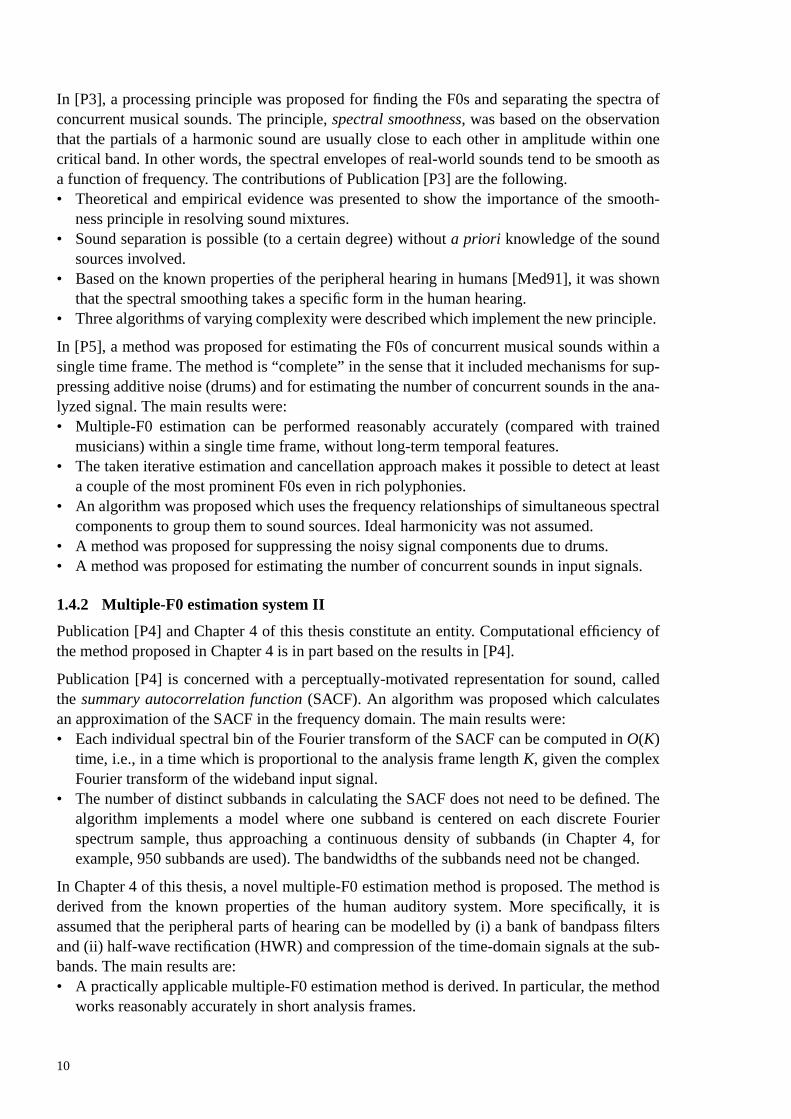
In [P3], a processing principle was proposed for finding the F0s and separating the spectra ofconcurrent musical sounds. The principle, spectral smoothness, was based on the observationthat the partials of a harmonic sound are usually close to each other in amplitude within onecritical band. In other words, the spectral envelopes of real-world sounds tend to be smooth asa function of frequency. The contributions of Publication [P3] are the following.• Theoretical and empirical evidence was presented to show the importance of the smooth-
ness principle in resolving sound mixtures.• Sound separation is possible (to a certain degree) without a priori knowledge of the sound
sources involved.• Based on the known properties of the peripheral hearing in humans [Med91], it was shown
that the spectral smoothing takes a specific form in the human hearing.• Three algorithms of varying complexity were described which implement the new principle.
In [P5], a method was proposed for estimating the F0s of concurrent musical sounds within asingle time frame. The method is “complete” in the sense that it included mechanisms for sup-pressing additive noise (drums) and for estimating the number of concurrent sounds in the ana-lyzed signal. The main results were:• Multiple-F0 estimation can be performed reasonably accurately (compared with trained
musicians) within a single time frame, without long-term temporal features.• The taken iterative estimation and cancellation approach makes it possible to detect at least
a couple of the most prominent F0s even in rich polyphonies.• An algorithm was proposed which uses the frequency relationships of simultaneous spectral
components to group them to sound sources. Ideal harmonicity was not assumed.• A method was proposed for suppressing the noisy signal components due to drums.• A method was proposed for estimating the number of concurrent sounds in input signals.
1.4.2 Multiple-F0 estimation system II
Publication [P4] and Chapter 4 of this thesis constitute an entity. Computational efficiency ofthe method proposed in Chapter 4 is in part based on the results in [P4].
Publication [P4] is concerned with a perceptually-motivated representation for sound, calledthe summary autocorrelation function (SACF). An algorithm was proposed which calculatesan approximation of the SACF in the frequency domain. The main results were:• Each individual spectral bin of the Fourier transform of the SACF can be computed in O(K)
time, i.e., in a time which is proportional to the analysis frame length K, given the complexFourier transform of the wideband input signal.
• The number of distinct subbands in calculating the SACF does not need to be defined. Thealgorithm implements a model where one subband is centered on each discrete Fourierspectrum sample, thus approaching a continuous density of subbands (in Chapter 4, forexample, 950 subbands are used). The bandwidths of the subbands need not be changed.
In Chapter 4 of this thesis, a novel multiple-F0 estimation method is proposed. The method isderived from the known properties of the human auditory system. More specifically, it isassumed that the peripheral parts of hearing can be modelled by (i) a bank of bandpass filtersand (ii) half-wave rectification (HWR) and compression of the time-domain signals at the sub-bands. The main results are:• A practically applicable multiple-F0 estimation method is derived. In particular, the method
works reasonably accurately in short analysis frames.
10

• It is shown that half-wave rectification at subbands amounts to the combined use of time-domain periodicity and frequency-domain periodicity for F0 extraction.
• Higher-order (unresolved) partials of a harmonic sound can be processed collectively. Esti-mation or detection of individual higher-order partials is not robust and should be avoided.
1.4.3 Musical meter estimation and sound onset detection
Publication [P2] proposed a method for onset detection, i.e., for the detection of the beginningsof discrete sound events in acoustic signals. The main contributions were:• A technique was described to cope with sounds that exhibit onset imperfections, i.e., the
amplitude envelope of which does not rise monothonically.• A psychoacoustic model of intensity coding was applied in order to find parameters which
allow robust one-by-one detection of onsets for a wide range of input signals.
In [P6], a method for musical-meter analysis was proposed. The analysis was performedjointly at three different time scales: at the temporally atomic tatum pulse level, at the tactuspulse level which corresponds to the tempo of a piece, and at the musical measure level. Themain contributions were:• The proposed method works robustly for different types of music and improved over two
state-of-the-art reference methods in simulations.• A technique was proposed for measuring the degree of musical accent as a function of time.
The technique was partially based on the ideas in [P2].• The paper confirmed an earlier result of Scheirer [Sch98] that comb-filter resonators are
suitable for metrical pulse analysis. Four different periodicity estimation methods wereevaluated and, as a result, comb-filters were the best in terms of simplicity vs. performance.
• Probabilistic models were proposed to encode prior musical knowledge regarding well-formed musical meters. The models take into account the dependencies between the threepulse levels and implement temporal tying between successive meter estimates.
1.5 Outline of the thesis
This thesis is organized as follows. Chapter 2 considers the musical meter estimation problem.A review of the previous work in this area is presented. This is followed by a short introductionto Publication [P6] where a novel method for meter estimation is proposed. Technical detailsand simulation results are not described but can be found in [P6]. A short conclusion is given todiscuss the achieved results and future work.
Chapter 3 introduces harmonic sounds and the different approaches that have been taken to theestimation of the fundamental frequency of isolated musical sounds. A model of the humanpitch perception is introduced and its benefits from the point of view of F0 estimation are dis-cussed.
Chapter 4 elaborates the pitch model introduced in Chapter 3 and, based on that, proposes apreviously unpublished method for estimating the F0s of multiple concurrent musical sounds.Also, Chapter 4 presents background material which serves as an introduction to [P4].
Chapter 5 reviews previous approaches to multiple-F0 estimation. Because this is the coreproblem in music transcription, the chapter can also be seen as an introduction to the potentialapproaches to music transcription in general.
Chapter 6 serves as an introduction to the other, problem-solving oriented method for multiple-
1 INTRODUCTION 11

F0 estimation. The method has been originally published in [P5] and is “complete” in the sensethat it includes mechanisms for suppressing additive noise and for estimating the number ofconcurrent sounds in the input signal. These are needed in order to process real-world musicsignals. Introduction to Publications [P1] and [P3] is given in Sec. 6.4. An epilogue in Sec. 6.5presents some criticism of the method.
Chapter 7 summarizes the main conclusions and discusses future work.
12

2 Musical meter estimation
This chapter reviews previous work on musical meter estimation and serves as an introductionto Publication [P6]. The concept musical meter was defined in Sec. 1.1. Meter analysis is anessential part of understanding music signals and an innate cognitive ability of humans evenwithout musical education. Virtually anybody is able to clap hands to music and it is not unu-sual to see a two-year old child swaying in time with music. From the point of view of musictranscription, meter estimation amounts to temporal segmentation of music according to cer-tain criteria.
Musical meter is a hierarchical structure, consisting of pulse sensations at different levels (timescales). In this thesis, three metrical levels are considered. The most prominent level is the tac-tus, often referred to as the foot tapping rate or the beat. Following the terminology of [Ler83],we use the word beat to refer to the individual elements that make up a pulse. A musical metercan be illustrated as in Fig. 3, where the dots denote beats and each sequence of dots corre-sponds to a particular pulse level. By the period of a pulse we mean the time duration betweensuccessive beats and by phase the time when a beat occurs with respect to the beginning of thepiece. The tatum pulse has its name stemming from “temporal atom” [Bil93]. The period ofthis pulse corresponds to the shortest durational values in music that are still more than inci-dentally encountered. The other durational values, with few exceptions, are integer multiplesof the tatum period and onsets of musical events occur approximately at a tatum beat. Themusical measure pulse is typically related to the harmonic change rate or to the length of arhythmic pattern. Although sometimes ambiguous, these three metrical levels are relativelywell-defined and span the metrical hierarchy at the aurally most important levels. Tempo of apiece is defined as the rate of the tactus pulse. In order that a meter would make sense musi-cally, the pulse periods must be slowly-varying and, moreover, each beat at the larger levelsmust coincide with a beat at all the smaller levels.
The concept phenomenal accent is important for meter analysis. Phenomenal accents areevents that give emphasis to a moment in music. Among these are the beginnings of all discretesound events, especially the onsets of long pitch events, sudden changes in loudness or timbre,and harmonic changes. Lerdahl and Jackendoff define the role of phenomenal accents in meterperception compactly by saying that “the moments of musical stress in the raw signal serve ascues from which the listener attempts to extrapolate a regular pattern” [Ler83,p.17].
Automatic estimation of the meter alone has several applications. A temporal framework facil-itates the cut-and-paste operations and editing of music signals. It enables synchronizationwith light effects, video, or electronic instruments, such as a drum machine. In a disc jockeyapplication, metrical information can be used to mark the boundaries of a rhythmic loop or to
96 97 98 99 100 101 102
TatumTactusMeasure
Figure 3. A musical signal with three metrical levels illustrated (reprinted from [P6]).
Time (seconds)
2 MUSICAL METER ESTIMATION 13

synchronize two or more percussive audio tracks. Meter estimation for symbolic (MIDI) datais required in time quantization, an indispensable subtask of score typesetting from keyboardinput.
2.1 Previous work
The work on automatic meter analysis originated from algorithmic models which tried toexplain how a human listener arrives at a particular metrical interpretation of a piece, given thatthe meter is not explicitly spelled out in music [Lee91]. The early models performed meterestimation for symbolic data, presented as an artificial impulse pattern or as a musical score[Ste77, Lon82, Lee85, Pov85]. In brief, all these models can be seen as being based on a set ofrules that are used to define what makes a musical accent and to infer the most natural meter.The rule system proposed by Lerdahl and Jackendoff in [Ler83] is the most complete, but isdescribed in verbal terms only. An extensive comparison of the early models has been given byLee in [Lee91], and later augmented by Desain and Honing in [Des99].
Table 1 lists characteristic attributes of more recent meter analysis systems. The systems canbe classified into two main categories according to the type of input they process. Some algo-rithms are designed for symbolic (MIDI) input whereas others process acoustic signals. Thecolumn, “evaluation material”, gives a more specific idea of the musical material that the sys-tems have been tested on. Another defining characteristic of different systems is the aim of themeter analysis. Many algorithms do not analyze meter at all time scales but at the tactus levelonly. Some others produce useful side-information, such as quantization of the onset and offsettimes of musical events. The columns “approach”, “mid-level representation” and “computa-tion” in Table 1 attempt to summarize the technique that is used to achieve the analysis result.More or less arbitrarily, three different approaches are discerned, one based on a set of rules,another employing a probabilistic model, and the third deriving the analysis methods mainlyfrom the signal processing domain. Mid-level representations refer to the data representationsthat are used between the input and the final analysis result. The column “computation” sum-marizes the strategy that is applied to search the correct meter among all possible meters.
2.1.1 Methods designed primarily for symbolic input (MIDI)
Rosenthal has proposed a system which processes realistic piano performances in the form ofMIDI files. His system attempted to emulate the human rhythm perception, including meterperception [Ros92]. Notable in his approach is that other auditory functions are taken intoaccount, too. During a preprocessing stage, notes are grouped into melodic streams and chords,and this information is utilized later on. Rosenthal applied a set of rules to rank and prune com-peting meter hypotheses and conducted a beam search to track multiple hypotheses throughtime. The beam-search strategy was originally proposed for pulse tracking by Allen and Dan-nenberg in [All90].
Parncutt has proposed a detailed model of meter perception based on systematic listening tests[Par94]. His algorithm computes the salience (weigth) of different metrical pulses based on aquantitative model for phenomenal accents and for pulse salience.
Apart from the rule-based models, a straightforward signal-processing oriented approach wastaken by Brown who performed metrical analysis of musical scores using the autocorrelationfunction [Bro93a]. The scores were represented as a time-domain signal (sampling rate
14

2M
USIC
AL
ME
TE
RE
STIM
AT
ION
15
R Evaluation material
R tracking
)
92 piano performances
Br nction
estimated)
19 classical scores
Lar ators
cking)
A few example analyses; straight-
forward to reimplement
P ern to accents Artificial synthesized patterns
T
Sle
r event occur-
r regularity
Example analyses; all music types;
source code available
Di istogram, then
(beam search)
222 MIDI files (expressive music);
10 audio files (sharp attacks);
source code available
R ation Two example analyses;
expressive performances
Ce
p
thods; balance
o continuity
216 polyphonic piano performances
of 12 Beatles songs; clave pattern
M
19
eam search);
city analysis;
sed in (1995)
85 pieces; pop music;
4/4 time signature
S ank of comb
n filter states
60 pieces with “strong beat”; all
music types; source code available
L stimation;
ch
Qualitative report; music with con-
stant tempo and sharp attacks
S
St
orm A few examples;
music with constant tempo
etogram), then
onous pattern
57 drum sequences of 2–10 s. in
duration; constant tempo
Kla comb filters,
ses using filter
rn matching
474 audio signals; all music types
Table 1: Characteristics of some meter estimation systems
eference Input Aim Approach Mid-level representation Computation
osenthal,
1992
MIDI meter, time
quantization
Rule-based,
model auditory
organization
At a preprocessing stage, notes are
grouped into streams and chords
Multiple-hypothesis
(beam search
own, 1993 score meter DSP Initialize a signal with zeros, then assign
note-duration values at their onset times
Autocorrelation fu
(only periods were being
ge, Kolen,
1994
MIDI meter DSP Initialize a signal with zeros, then
assign unity values at note onsets
Network of oscill
(period and phase lo
arncutt,
1994
score meter,
accent
modeling
Rule-based,
based on listen-
ing tests
Phenomenal accent model for individual
events (event parameters: length, loud-
ness, timbre, pitch)
Match an isochronous patt
emperley,
ator, 1999
MIDI meter, time
quantization
Rule-based Apply discrete time-base, assign each
event to the closest 35ms time-frame
Viterbi; “cost functions” fo
rence, event length, mete
xon, 2001 MIDI,
audio
tactus Rule-based,
heuristic
MIDI: parameters of MIDI-events.
Audio: compute overall amplitude enve-
lope, then extract onset times
First find periods using IOI h
phases with multiple-agents
aphael,
2001
MIDI,
audio
tactus, time
quantization
Probabilistic
generative model
Only onset times are used Viterbi; MAP estim
mgil, Kap-
en, 2003
MIDI tactus, time
quantization
Probabilistic
generative model
Only onset times are used Sequential Monte Carlo me
score complexity vs. temp
Goto,
uraoka,
95, 1997
audio meter DSP Fourier spectra, onset components (time,
reliability, frequency range)
Multiple tracking agents (b
IOI histogram for periodi
pre-stored drum patterns u
cheirer,
1998
audio tactus DSP Amplitude-envelope signals at six
subbands
First find periods using a b
filters, then phases based o
aroche,
2001
audio tactus,
swing
Probabilistic Compute overall “loudness” curve, then
extract onset times and weights
Maximum-likelihood e
exhaustive sear
ethares,
aley, 2001
audio meter DSP RMS-energies at 1/3-octave subbands Periodicity transf
Gouyon
al., 2002
audio tatum DSP Compute overall amplitude envelope,
then extract onsets times and weights
First find periods (IOI hist
phases by matching isochr
puri et al.,2003
audio meter DSP,
probabilistic
back-end
Degree of accentuation as a function of
time at four frequency ranges
First find periods (bank of
Viterbi back-end), then pha
states and rhythmic patte
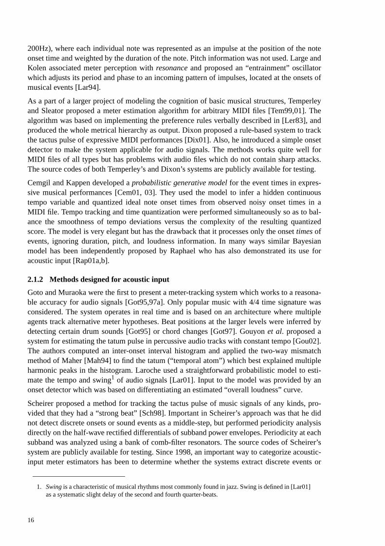
200Hz), where each individual note was represented as an impulse at the position of the noteonset time and weighted by the duration of the note. Pitch information was not used. Large andKolen associated meter perception with resonance and proposed an “entrainment” oscillatorwhich adjusts its period and phase to an incoming pattern of impulses, located at the onsets ofmusical events [Lar94].
As a part of a larger project of modeling the cognition of basic musical structures, Temperleyand Sleator proposed a meter estimation algorithm for arbitrary MIDI files [Tem99,01]. Thealgorithm was based on implementing the preference rules verbally described in [Ler83], andproduced the whole metrical hierarchy as output. Dixon proposed a rule-based system to trackthe tactus pulse of expressive MIDI performances [Dix01]. Also, he introduced a simple onsetdetector to make the system applicable for audio signals. The methods works quite well forMIDI files of all types but has problems with audio files which do not contain sharp attacks.The source codes of both Temperley’s and Dixon’s systems are publicly available for testing.
Cemgil and Kappen developed a probabilistic generative model for the event times in expres-sive musical performances [Cem01, 03]. They used the model to infer a hidden continuoustempo variable and quantized ideal note onset times from observed noisy onset times in aMIDI file. Tempo tracking and time quantization were performed simultaneously so as to bal-ance the smoothness of tempo deviations versus the complexity of the resulting quantizedscore. The model is very elegant but has the drawback that it processes only the onset times ofevents, ignoring duration, pitch, and loudness information. In many ways similar Bayesianmodel has been independently proposed by Raphael who has also demonstrated its use foracoustic input [Rap01a,b].
2.1.2 Methods designed for acoustic input
Goto and Muraoka were the first to present a meter-tracking system which works to a reasona-ble accuracy for audio signals [Got95,97a]. Only popular music with 4/4 time signature wasconsidered. The system operates in real time and is based on an architecture where multipleagents track alternative meter hypotheses. Beat positions at the larger levels were inferred bydetecting certain drum sounds [Got95] or chord changes [Got97]. Gouyon et al. proposed asystem for estimating the tatum pulse in percussive audio tracks with constant tempo [Gou02].The authors computed an inter-onset interval histogram and applied the two-way mismatchmethod of Maher [Mah94] to find the tatum (“temporal atom”) which best explained multipleharmonic peaks in the histogram. Laroche used a straightforward probabilistic model to esti-mate the tempo and swing1 of audio signals [Lar01]. Input to the model was provided by anonset detector which was based on differentiating an estimated “overall loudness” curve.
Scheirer proposed a method for tracking the tactus pulse of music signals of any kinds, pro-vided that they had a “strong beat” [Sch98]. Important in Scheirer’s approach was that he didnot detect discrete onsets or sound events as a middle-step, but performed periodicity analysisdirectly on the half-wave rectified differentials of subband power envelopes. Periodicity at eachsubband was analyzed using a bank of comb-filter resonators. The source codes of Scheirer’ssystem are publicly available for testing. Since 1998, an important way to categorize acoustic-input meter estimators has been to determine whether the systems extract discrete events or
1. Swing is a characteristic of musical rhythms most commonly found in jazz. Swing is defined in [Lar01]as a systematic slight delay of the second and fourth quarter-beats.
16

onset times as a middle-step or not. The meter estimator of Sethares and Staley is in manyways similar to Scheirer’s method, with the difference that a periodicity transform was used forperiodicity analysis instead of a bank of comb filters [Set01].
2.1.3 Summary
To summarize, most of the earlier work on meter estimation has concentrated on symbolic(MIDI) data and typically analyzed the tactus pulse only. Some of the systems ([Lar94],[Dix01], [Cem03], [Rap01b]) can be immediately extended to process audio signals byemploying an onset detector which extracts the beginnings of discrete acoustic events from anaudio signal. Indeed, the authors of [Dix01] and [Rap01b] have introduced an onset detectorthemselves. Elsewhere, onset detection methods have been proposed that are based on using anauditory model [Moe97], subband power envelopes [P2], support vector machines [Dav02],neural networks [Mar02], independent component analysis [Abd03], or complex-domainunpredictability [Dux03]. However, if a meter estimator has been originally developed forsymbolic data, the extended system is usually not robust to diverse acoustic material (e.g. clas-sical vs. rock music) and cannot fully utilize the acoustic cues that indicate phenomenalaccents in music signals.
There are a few basic problems that a meter estimator needs to address to be successful. First,the degree of musical accentuation as a function of time has to be measured. In the case ofaudio input, this has much to do with the initial time-frequency analysis and is closely relatedto the problem of onset detection. Some systems measure accentuation in a continuous manner[Sch98, Set01], whereas others extract discrete events [Got95,97, Gou02, Lar01]. Secondly,the periods and phases of the underlying metrical pulses have to be estimated. The methodswhich detect discrete events as a middle step have often used inter-onset interval histogramsfor this purpose [Dix01, Got95,97, Gou02]. Thirdly, a system has to choose the metrical levelwhich corresponds to the tactus or some other specially designated pulse level. This may takeplace implicitly, or by using a prior distribution for pulse periods [Par94], or by applying rhyth-mic pattern matching [Got95]. Tempo halving or doubling is a symptom of failing to do this.
2.2 Method proposed in Publication [P6]
The aim of the method proposed in [P6] is to estimate the meter of acoustic musical signals atthree levels: at the tactus, tatum, and measure-pulse levels. The target signals are not restrictedto any particular music type but all the main genres, including classical and jazz music, are rep-resented in the validation database.
An overview of the method is shown in Fig. 4. For the time-frequency analysis part, a newtechnique is proposed which aims at measuring the degree of accentuation in music signals.The technique is robust to diverse acoustic material and can be seen as a synthesis and general-ization of two earlier state-of-the-art methods [Got95] and [Sch98]. In brief, preliminary time-frequency analysis is conducted using a quite large number of subbands and by meas-uring the degree of spectral change at these channels. Then, adjacent bands are combined toarrive at a smaller number of “registral accent signals” for which periodicity analy-sis is carried out. This approach has the advantage that the frequency resolution suffices todetect harmonic changes but periodicity analysis takes place at wider bands. Combining a cer-tain number of adjacent bands prior to the periodicity analysis improves the analysis accuracy.Interestingly, neither combining all the channels before periodicity analysis, , nor ana-
b0 20>
3 c0 5≤ ≤
c0 1=
2 MUSICAL METER ESTIMATION 17

lyzing periodicity at all channels, , is an optimal choice but using a large number ofbands in the preliminary time-frequency analysis (we used ) and three or four regis-tral channels leads to the most reliable analysis.
Periodicity analysis of the registral accent signals is performed using a bank of comb filter res-onators very similar to those used by Scheirer in [Sch98]. Figure 5 illustrates the energies ofthe comb filters as a function of their feedback delay, i.e., period, . The energies are shownfor two types of artificial signals, an impulse train and a white-noise signal. It is important tonotice that all resonators that are in rational-number relations to the period of the impulse train(24 samples) show response to it. This turned out to be important for meter analysis. In the caseof an autocorrelation function, for example, only integer multiples of 24 come up and, in orderto achieve the same meter estimation performance, an explicit postprocessing step (“enhanc-ing”) is necessary where the autocorrelation function is progressively decimated and summedwith the original autocorrelation function.
Periods
Filter states
Figure 4. Overview of the meter estimation method. The two intermediate data represen-tations are registral accent signals at band c and metrical pulse strengths forresonator period at time n. (Reprinted from [P6].)
vc n( ) s τ n,( )τ
Time-
frequency
analysis
Comb filter
resonators
Meter
Musicsignal
vc n( ) s τ n,( )
Com
bin
e
Probabilistic
model for
pulse periods
PhasesPhase
model
c0 b0=b0 36=
c0
0 24 48 72 960
0.2
0.4
0.6
0.8
1
0 24 48 72 960
0.2
0.4
0.6
0.8
1
0 24 48 72 960
0.2
0.4
0.6
0.8
1
0 24 48 72 960
0.2
0.4
0.6
0.8
1
Figure 5. Output energies of comb filter resonators as a function of their feedback delay(period) . The energies are shown for an impulse train with a period-length 24 samples(left) and for a white noise signal (right). Upper panels show the raw output energies andthe lower panels the energies after a specific normalization. (Reprinted from [P6].)
τ
Delay τ (samples) Delay τ (samples)
Ene
rgy
Nor
mal
ized
ene
rgy
Delay τ (samples) Delay τ (samples)
Ene
rgy
Nor
mal
ized
ene
rgy
τ
18

Before we ended up using comb filters, four different period estimation algorithms were evalu-ated: the above-mentioned “enhanced” autocorrelation, enhanced YIN method of de Cheveignéand Kawahara [deC02], different types of comb-filter resonators [Sch98], and banks of phase-locking resonators [Lar94]. As an important observation, three out of the four period estima-tion methods performed equally well after a thorough optimization. This suggests that the keyproblems in meter estimation are in measuring phenomenal accentuation and in modelinghigher-level musical knowledge, not in finding exactly the correct period estimator. A bank ofcomb filter resonators was chosen because it is the least complex among the three best-per-forming algorithms.
The comb filters serve as feature extractors for two probabilistic models. One model is used toestimate the period-lengths of metrical pulses at different levels. The other model is used toestimate the corresponding phases (see Fig. 4). The probabilistic models encode prior musicalknowledge regarding well-formed musical meters. In brief, the models take into account thedependencies between different pulse levels (tatum, tactus, and measure) and, additionally,implement temporal tying between successive meter estimates. As shown in the evaluation sec-tion of [P6], this leads to a more reliable and temporally stable meter tracking.
2.3 Results and criticism
The method proposed in [P6] is quite successful in estimating the meter of different kinds ofmusic signals and improved over two state-of-the-art reference methods in simulations. Simi-larly to human listeners, computational meter estimation was easiest at the tactus pulse level.For the measure pulse, period estimation can be done equally robustly but estimating the phaseis less straightforward. This appears to be due to the basic decision that multiple-F0 analysiswas not employed prior to the meter analysis. Since the measure pulse is typically related tothe harmonic change rate, F0 information could potentially lead to significantly better meterestimation at the measure-pulse level. For the tatum pulse, in turn, phase estimation does notrepresent a problem but deciding the period is difficult both for humans and for the proposedmethod.
The critical elements of a meter estimation system appear to be the initial time-frequency anal-ysis part which measures musical accentuation as a function of time and the (often implicit)internal model which represents primitive musical knowledge. The former is needed to providerobustness for diverse instrumentations in e.g. classical, rock, and electronic music. The latteris needed to achieve temporally stable meter tracking and to fill in parts where the meter is onlyfaintly implied by the musical surface. A challenge in the latter part is to develop a modelwhich is generic for various genres, for example for jazz and classical music. The model pro-posed in [P6] describes sufficiently low-level musical knowledge to generalize over differentgenres.
2 MUSICAL METER ESTIMATION 19

20
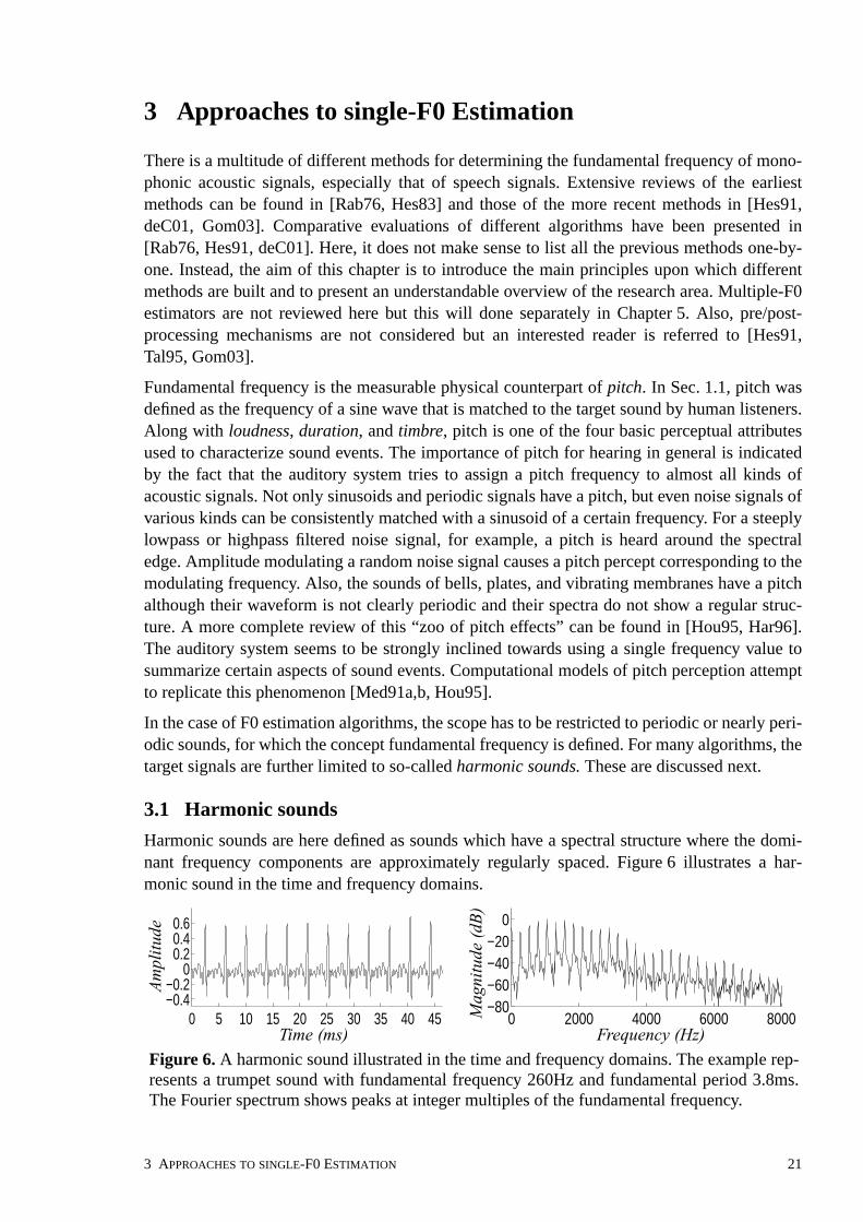
3 Approaches to single-F0 Estimation
There is a multitude of different methods for determining the fundamental frequency of mono-phonic acoustic signals, especially that of speech signals. Extensive reviews of the earliestmethods can be found in [Rab76, Hes83] and those of the more recent methods in [Hes91,deC01, Gom03]. Comparative evaluations of different algorithms have been presented in[Rab76, Hes91, deC01]. Here, it does not make sense to list all the previous methods one-by-one. Instead, the aim of this chapter is to introduce the main principles upon which differentmethods are built and to present an understandable overview of the research area. Multiple-F0estimators are not reviewed here but this will done separately in Chapter 5. Also, pre/post-processing mechanisms are not considered but an interested reader is referred to [Hes91,Tal95, Gom03].
Fundamental frequency is the measurable physical counterpart of pitch. In Sec. 1.1, pitch wasdefined as the frequency of a sine wave that is matched to the target sound by human listeners.Along with loudness, duration, and timbre, pitch is one of the four basic perceptual attributesused to characterize sound events. The importance of pitch for hearing in general is indicatedby the fact that the auditory system tries to assign a pitch frequency to almost all kinds ofacoustic signals. Not only sinusoids and periodic signals have a pitch, but even noise signals ofvarious kinds can be consistently matched with a sinusoid of a certain frequency. For a steeplylowpass or highpass filtered noise signal, for example, a pitch is heard around the spectraledge. Amplitude modulating a random noise signal causes a pitch percept corresponding to themodulating frequency. Also, the sounds of bells, plates, and vibrating membranes have a pitchalthough their waveform is not clearly periodic and their spectra do not show a regular struc-ture. A more complete review of this “zoo of pitch effects” can be found in [Hou95, Har96].The auditory system seems to be strongly inclined towards using a single frequency value tosummarize certain aspects of sound events. Computational models of pitch perception attemptto replicate this phenomenon [Med91a,b, Hou95].
In the case of F0 estimation algorithms, the scope has to be restricted to periodic or nearly peri-odic sounds, for which the concept fundamental frequency is defined. For many algorithms, thetarget signals are further limited to so-called harmonic sounds. These are discussed next.
3.1 Harmonic sounds
Harmonic sounds are here defined as sounds which have a spectral structure where the domi-nant frequency components are approximately regularly spaced. Figure 6 illustrates a har-monic sound in the time and frequency domains.
0 2000 4000 6000 8000−80−60−40−20
0
0 5 10 15 20 25 30 35 40 45−0.4−0.2
00.20.40.6
Time (ms) Frequency (Hz)
Am
plitu
de
Mag
nitu
de (
dB)
Figure 6. A harmonic sound illustrated in the time and frequency domains. The example rep-resents a trumpet sound with fundamental frequency 260Hz and fundamental period 3.8ms.The Fourier spectrum shows peaks at integer multiples of the fundamental frequency.
3 APPROACHES TO SINGLE-F0 ESTIMATION 21

For an ideal harmonic sound, the frequencies of the overtone partials (harmonics) are integermultiples of the F0. In the case of many real-world sound production mechanisms, however,the partial frequencies are not in exact integral ratios although the general structure of the spec-trum is similar to that in Fig. 6. For stretched strings, for example, the frequencies of the par-tials obey the formula
, (3.1)
where F is the fundamental frequency, h is harmonic index (partial number), and is inharmo-nicity factor [Fle98, p.363]. Figure 7 shows the spectrum of a vibrating piano string with theideal harmonic frequencies indicated above the spectrum. The inharmonicity phenomenonappears so that the higher-order partials have been shifted upwards in frequency. However, thestructure of the spectrum is in general very similar to that in Fig. 6 and the sound belongs to theclass of harmonic sounds. Here, the inharmonicity is due to the stiffness of real strings whichcontributes as a restoring force along with the string tension [Jär01]. As a consequence, thestrings are dispersive, meaning that different frequencies propagate with different velocities inthe string. Figure 8 illustrates the deviation of the frequency from the ideal harmonic posi-tion, when a moderate inharmonicity value is substituted to (3.1).
Figure 9 shows an example of a sound which does not belong to the class of harmonic soundsalthough it is nearly periodic in time domain and has a clear pitch. In Western music, malletpercussion instruments are a case in point: these instruments produce pitched sounds which arenot harmonic. The vibraphone sound in Fig. 9 represents this family of instruments.
The methods proposed in this thesis are mainly concerned with harmonic sounds (not assum-ing ideal harmonicity, however) and do not operate quite as reliably for nonharmonic sounds,such as that illustrated in Fig. 9. This limitation is not very severe in Western music, though.
f h hF 1 β h2 1–( )+=
β
0 500 1000 1500 2000 2500 3000 3500 4000−80−60−40−20
020
1 510
1520
25
Figure 7. Spectrum of a vibrating piano string ( Hz). Ideal harmonic locations arenumbered and indicated with “+” marks above the spectrum. The inharmonicity phenome-non (i.e., non-ideal harmonicity) shifts the 24th harmonic partial to the position of the 25thideal harmonic.
F 156=
Frequency (Hz)
Mag
nitu
de (
dB)
1 5 10 15 20 250
100
200
300
Figure 8. Deviation of the partial frequency from the ideal ( ), when (3.1) withHz and moderate inharmonicity factor is used to calculate .
f h hFF 100= β 0.0004= f h
Dev
iatio
n (H
z)
Harmonic index h
f hβ 0.0004=
22

Table 2 lists Western musical instruments that do or do not produce harmonic sounds. Thefamily of mallet percussion instruments is not very commonly used in contemporary music.
3.2 Taxonomy of F0 estimation methods
F0 estimation algorithms do not only differ in technical details but in regard to the very infor-mation that the calculations are based on. That is, there is no single obvious way of calculatingthe F0 of an acoustic signal which is not perfectly periodic and may be presented in back-ground noise. Another problem is that often the model-level assumptions of the algorithmshave not been explicitly stated, making it difficult to compare different algorithms and to com-bine their advantages. To this end, some categorization and model-level analysis of variousmethods is presented here.
In psychoacoustics, computational models of pitch perception have been traditionally classi-fied as either place models or temporal models. An excellent introduction to these competingtheories and their supporting evidence can be found in [Har96]. A convincing attempt to unifythe two theories (a “unitary model”) has been presented by Meddis and colleagues in[Med91a,b, 97].
In the case of practical F0 estimation methods, a different categorization is more useful. Algo-rithms are here grouped to those that look for frequency partials at harmonic spectral locationsand to those that observe spectral intervals (frequency intervals) between partials. The under-lying idea of both of these categories can be understood by looking at Fig. 6 and is described inmore detail in the next two subsections. Algorithms which measure periodicity of the time-
0 1000 2000 3000 4000 5000 6000 7000
−80−60−40−20
020 1.0 4.0
10.38.1 16.613.4 21.8 25.5
0 10 20 30 40
−0.5
0
0.5
Figure 9. A vibraphone sound with fundamental frequency 260Hz illustrated in the timeand frequency domains. In the right panel, frequencies of the most dominant spectral com-ponents are shown in relation to the F0.
Frequency (Hz)
Mag
nitu
de (
dB)
Time (ms)
Am
plitu
de
Table 2: Western musical instruments which do or do not produce harmonic sounds.
Produced sounds Instrument family Instruments involved
Harmonic
String instruments Piano, guitars, bowed strings (violin etc.)Reed instruments Clarinets, saxophones, oboe, bassoonBrass instruments Trumpet, trombone, tuba, english/french horn
Flutes Flute, bass flute, piccolo, organPipe organs Flue pipes and reed pipes
Human voice (singing) Voiced phonemes
Not harmonicMallet percussions Marimba, xylophone, vibraphone, glockenspiel
Drums Kettle drums, tom-toms, snare drums, cymbals
3 APPROACHES TO SINGLE-F0 ESTIMATION 23

domain signal belong to the first category. Algorithms which measure periodicity of the Fou-rier spectrum belong to the latter category. Algorithms which measure periodicity of the time-domain amplitude envelope represent a tradeoff between the two classes and are described inSec. 3.5. Recent models of human pitch perception are of this kind: both spectral locations andspectral intervals are important in hearing. In the following, representative variants from eachcategory are introduced and analyzed in order to describe their properties and advantages.
3.3 Spectral-location type F0 estimators
3.3.1 Time-domain periodicity analysis methods
Time-domain autocorrelation function (ACF) based algorithms are among the most frequentlyused F0 estimators (see e.g. [Bro91, Tal95]). As pointed out by Tolonen and Karjalainen in[Tol00], ACF-based F0 estimators have close model-level similarities with cepstrum-based F0estimators [Nol67], and there is a continuum between them. This becomes evident when calcu-lating ACF of a time-domain signal via the discrete Fourier transform (DFT) and itsinverse (IDFT) as
. (3.2)
Definition of the cepstrum of x(n) is very analogous to (3.2) and is obtained by replacingthe second power with a logarithm function. The difference between the ACF and cepstrum-based F0 estimators is quantitative. Raising the magnitude spectrum to the second poweremphasizes spectral peaks in relation to noise but, on the other hand, further aggravates spec-tral peculiarities of the target sound. Applying the logarithm function causes the opposite forboth. And indeed, ACF-based F0 estimators have been reported to be relatively noise immunebut sensitive to formant structures in speech: especially the first and the strongest formant maymislead the algorithm [Rab76, Tal95]. On the contrary, cepstrum-based F0 estimators performrelatively poorly in noise, but well for exotic sounds [Rab76]. As a tradeoff, Tolonen et al. sug-gest using a “generalized autocorrelation function” where the second power is replaced with areal-valued exponent (0.67 in their case) [Tol00].
Both ACF and cepstrum-based F0 detectors are implicit realizations of a model which empha-sizes frequency partials at harmonic locations of the magnitude spectrum. This can be seen bywriting the ACF in terms of the Fourier spectrum of a a real-valued input signal as
, (3.3)
where K is the length of the transform frame. The above formula is equivalent to (3.2).Figure 10 illustrates the calculations in the case when corresponds to the true period of theexample sound. Squared magnitude-spectrum components are weighted according to theirspectral locations and then summed. Thus we call ACF and cepstrum-based methods spectrallocation type F0 estimators.
Recently, a conceptually simple and very accurate F0 estimation method was proposed byde Cheveigné and Kawahara in [deC02]. Their algorithm is called “YIN” and is based on theACF with certain modifications. The novelty of the method culminates to a specific normaliza-tion of the autocorrelation function which reduces the number of free parameters instead ofincreasing it. In [deC01], the method was thoroughly evaluated and compared with previous
x n( )
r τ( ) IDFT DFT x n( )[ ] 2{ }=
c τ( )
X k( )
r τ( ) 1K---- 2πτk
K------------ cos X k( ) 2
k 0=
K 1–
∑=
τ
24

methods using a large database of speech signals. The usability of the method for music tran-scription has been evaluated by us in [Vii03] and in Publication [P5].
Autocorrelation-based methods are closely related to methods which average the absolute dif-ference between a signal and its delayed version. An interesting generalization over the time-delay based methods has been recently proposed by Terez who applied state-space embeddingin searching the time delay with which the signal resembles itself [Ter02].
3.3.2 Harmonic pattern matching in frequency domain
Another way of weighting frequency components according to their spectral locations is toperform explicit pattern matching in the frequency domain. In [Bro92b], Brown proposed amethod where an input sound is first analyzed by simulating a 1/24th-octave filterbank. Thisleads to a spectral representation where the frequency components are logarithmically spaced.In log-frequency domain, the partials of a harmonic sound have a spacing which is independentof the F0 of the sound. For example, the distance between the second and the third harmonicpartial is regardless of the F0. As a consequence, F0 estimation can be performed bycross-correlating the vector of filterbank energies with an ideal harmonic pattern where unityvalues are assigned to harmonic positions and zeros elsewhere. The maximum of the cross cor-relation function indicates the position of the fundamental frequency.
A maximum-likelihood spectral pattern matching F0 estimator was proposed by Doval andRodet in [Dov91, 93]. The authors used a set of sinusoidal partials to represent the spectrum ofan input sound and a F0 was then sought for which best explained the observed partials. Thiswas done in a Bayesian manner so that Gaussian functions centered on each multiple of ahypothesized F0 were used to represent the likelihood of observing the partials given the F0candidate. Supplementary non-harmonic and noisy spectral components were separately mod-eled.
Another completely different and interesting spectral pattern matching approach is the two-way mismatch method of Maher and Beauchamp [Mah94]. In their method, the F0 is chosen tominimize discrepancies between observed frequency components and harmonic frequenciesgenerated by trial F0 values. The first mismatch measure is calculated as an average of the fre-quency differences between each observed partial and its nearest neighbour among the pre-dicted harmonic frequencies. This is combined with a mismatch measure calculated byaveraging the frequency differences between each predicted harmonic frequency and its near-est neighbour among the observed partials.
0 500 1000 1500 2000 2500 3000 3500 4000 0
−1 0 1
Figure 10. Solid line illustrates the power spectrum of a trumpet sound. Dashed line showsthe weights of ACF calculation in (3.3) when corresponds to the funda-mental period of the example sound. The two curves are displaced vertically for clarity.
2πτk K⁄( )cos τ
Frequency (Hz)
Pow
er;
wei
ghts
3 2⁄( )ln
3 APPROACHES TO SINGLE-F0 ESTIMATION 25

3.3.3 A shortcoming of spectral-location type F0 estimators
A major shortcoming of the spectral-location oriented F0 estimation methods is that they arenot able to handle non-ideal harmonic sounds appropriately. As described in Sec. 3.1, the par-tials of real physical vibrators cannot be assumed to be found exactly at harmonic spectrumpositions. The spectrum of a piano sound in Fig. 7 illustrates this situation. Inharmonicity isnot a big concern in speech processing, but is immediately met when analyzing musical soundsat a wide frequency band. The methods described in the next section are advantageous in thisrespect.
3.4 Spectral-interval type F0 estimators
The spectrum autocorrelation method and its variants have been successfully used in severalF0 estimators (see e.g. [Lah87, Kun96]). The idea is derived from the observation that a peri-odic but non-sinusoidal signal has a periodic magnitude spectrum, the period of which is theF0. In its simplest form, the autocorrelation function over the positive frequencies of aK-length magnitude spectrum can be calculated as
. (3.4)
The information on which the above equation bases F0 calculations is fundamentally differentfrom that of a time-domain ACF or cepstrum-based F0 detector. Any two frequency compo-nents with a certain spectral interval support the corresponding F0. This means that the spec-trum can be arbitrarily shifted without affecting the output value. Different kinds ofpreprocessing can be done for the spectrum before the periodicity analysis. For example,Kunieda et al. compress the magnitude spectrum with a logarithm function and then removethe spectral trend by highpass liftering1 [Kun96]. Lahat et al. apply a bank of bandpass liftersprior to the periodicity analysis [Lah87].
Building F0 calculations upon the intervals between frequency partials works better for soundsthat exhibit inharmonicities. Even though the intervals do not remain constant, they are morestable than the locations of the partials, which shift cumulatively, as can be seen in (3.1) and inFig. 8.
Another interesting difference between spectral-location and spectral-interval basedapproaches is that the former methods are prone to errors in F0 halving and the latter to errorsin F0 doubling. As an example, consider the time-domain ACF estimator (spectral-locationtype method). The time-domain signal is periodic at half the F0 rate (twice the fundamentalperiod) and the harmonic partials of a sound match the locations of even harmonics of a twotimes lower sound. In the case of the frequency-domain ACF estimator (spectral-interval typemethod), the magnitude spectrum is periodic at double the F0 rate but shows no periodicity athalf the F0 rate.
1. Liftering refers to the process of convolving the sequence of magnitude-spectrum samples with theimpulse response of the specified filter.
r m( )
r m( ) 2K---- X k( ) X k m+( )
k 0=
K 2⁄ m– 1–
∑=
26
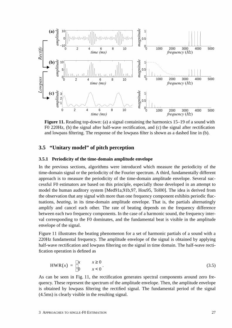
3.5 “Unitary model” of pitch perception
3.5.1 Periodicity of the time-domain amplitude envelope
In the previous sections, algorithms were introduced which measure the periodicity of thetime-domain signal or the periodicity of the Fourier spectrum. A third, fundamentally differentapproach is to measure the periodicity of the time-domain amplitude envelope. Several suc-cessful F0 estimators are based on this principle, especially those developed in an attempt tomodel the human auditory system [Med91a,91b,97, Hou95, Tol00]. The idea is derived fromthe observation that any signal with more than one frequency component exhibits periodic fluc-tuations, beating, in its time-domain amplitude envelope. That is, the partials alternatinglyamplify and cancel each other. The rate of beating depends on the frequency differencebetween each two frequency components. In the case of a harmonic sound, the frequency inter-val corresponding to the F0 dominates, and the fundamental beat is visible in the amplitudeenvelope of the signal.
Figure 11 illustrates the beating phenomenon for a set of harmonic partials of a sound with a220Hz fundamental frequency. The amplitude envelope of the signal is obtained by applyinghalf-wave rectification and lowpass filtering on the signal in time domain. The half-wave recti-fication operation is defined as
. (3.5)
As can be seen in Fig. 11, the rectification generates spectral components around zero fre-quency. These represent the spectrum of the amplitude envelope. Then, the amplitude envelopeis obtained by lowpass filtering the rectified signal. The fundamental period of the signal(4.5ms) is clearly visible in the resulting signal.
0 1000 2000 3000 4000 50000
0.5
1
0 2 4 6 8 10−10
0
10
0 1000 2000 3000 4000 50000
0.5
1
0 2 4 6 8 100
5
10
0 1000 2000 3000 4000 50000
0.5
1
0 2 4 6 8 10
123
Figure 11. Reading top-down: (a) a signal containing the harmonics 15–19 of a sound withF0 220Hz, (b) the signal after half-wave rectification, and (c) the signal after rectificationand lowpass filtering. The response of the lowpass filter is shown as a dashed line in (b).
frequency (Hz)time (ms)
Rec
tify
time (ms)
time (ms)
frequency (Hz)
frequency (Hz)
mag
nitu
dem
agni
tude
mag
nitu
de
ampl
itude
ampl
itude
ampl
itudeLo
wpa
ss
(a)
(b)
(c)
HWR x( )x x 0≥0 x 0<
=
3 APPROACHES TO SINGLE-F0 ESTIMATION 27

At first it seems that analyzing the periodicity of the amplitude envelope leads to a spectral-interval type F0 estimator. However, the principle of rectification and lowpass filtering allowsan elegant tradeoff between the spectral-location and spectral-interval type information. This isachieved by tuning the cutoff frequency of the lowpass filter in Fig. 11. If the cutoff frequencyof the lowpass filter is risen so that the filter passes the spectral components of the original nar-rowband signal, a subsequent periodicity analysis (ACF computation, for example) utilizesboth spectral-location and spectral-interval information. This is because the spectrum after rec-tification contains partials at frequencies which correspond to the spectral locations of partialsin the input signal and to the spectral intervals between the partials. In human hearing, a trade-off between the two types of information is achieved using this kind of representation. This isdescribed in more detail in the following.
3.5.2 Unitary model of pitch perception
Meddis and colleagues have proposed a computational model of human pitch perception wherethe periodicity of the amplitude envelope is analyzed at the outputs of a bank of bandpass fil-ters [Med91a,b, 97]. The roots of the model are in the early work of Licklider [Lic51]. Simula-tion experiments with the model have shown that this single model (hence the name “unitary”)is capable of reproducing a wide range of phenomena in human pitch perception, thus reconcil-ing discrepancies between competing psychoacoustic theories (as mentioned in Sec. 3.2). Forconvenience, this model is referred to simply as “unitary model” in the following.
The unitary model consists of the following processing steps [Med97]:
1. An acoustic input signal is passed though a bank of bandpass filters which represent the fre-quency selectivity of the inner ear. The bands (or, channels) are approximately uniformlydistributed on a logarithmic frequency scale. Typically, 40–128 filters with partly overlap-ping passbands are applied.
2. The signal at each channel is compressed, half-wave rectified, and lowpass filtered.3. Periodicity estimation within channels is carried out by calculating short-time autocorrela-
tion functions.4. The ACF estimates are linearly summed across channels to obtain a summary autocorrela-
tion function (SACF) defined as
(3.6)
where is the autocorrelation function at time t in subband c. The maximum value ofis typically used to determine the time delay (lag) which corresponds to the pitch period
at time t.
The first two steps of the above algorithm correspond to the peripheral parts of hearing whichproduce a signal to the auditory nerve. There is a wide consensus concerning the general prop-erties of these processing steps because the signal in the auditory nerve can be directly meas-ured. The steps 3 and 4 are more controversial since they represent processing which takesplace in the central nervous system and is not directly observable. Particularly the use of theACF for periodicity estimation has been a subject to criticism since no nervous units have beenfound that could implement ACF as such (see e.g. [Har96, p.3498]) and some experimentalevidence contradicts the ACF [Kae98, 01]. The authors themselves admit that the ACF is notnecessarily the exact mechanism that the auditory system uses. In [Med91a, p. 2879], theywrite: “The model, therefore, remains neutral on the exact mechanism whereby temporal infor-
st τ( ) rt c, τ( )c∑=
rt c, τ( )st τ( )
28

mation is extracted from the activity of the auditory-nerve fibers - - -” (activity of the auditory-nerve fibers is modelled by the amplitude envelopes). The overall processing chain, however,has been very successful in reproducing phenomena in human hearing and the model thereforeprevails until a better one is found. A viable substitute for ACF has not been found despitesome attempts e.g. in [Bra99, 00].
Envelope periodicity is in practice always analyzed at subbands and the results are then com-bined in the end. This applies not only to the unitary pitch model but also to practical F0extraction methods. It should be noted that analyzing the periodicity of the time-domain signalitself or the Fourier spectrum at subchannels (and then summing) does not make sense sincethis is equivalent to performing the periodicity analysis directly for the wideband signal.
3.5.3 Attractive properties of the unitary model
The unitary model has a number of properties which are particularly attractive from the pointof view of F0 estimation. Furthermore, these properties stem already from the first two (widelyaccepted) processing steps which produce the signal traveling in the auditory nerve. Threeproperties are discussed in the following.
First, the model provides a psychoacoustically plausible way of weighting the spectral-locationand spectral-interval type information in F0 estimation. The half-wave rectification operationretains the spectral components of the input signal around fc (center frequency of the bandpassfilter at channel c) but, additionally, generates the spectrum of the amplitude envelope aroundzero frequency (in addition, harmonic distortion is generated at integer multiples of fc; this isdiscussed later). The spectrum around fc represent spectral-location type information whereasthe spectral components of the amplitude envelope correspond to intervals between the partialsin the input signal as described in Sec. 3.5.1. The subsequent ACF computation performs pat-tern matching on this spectrum, as illustrated in Fig. 10.
The magnitude response of the lowpass filter (illustrated in Fig. 11) determines the balancebetween the two types of information. In the unitary model, the lowpass filter is common to allsubbands and is typically designed to pass signal components below about 1kHz and to have asmooth transition band so that signal components above 1kHz are increasingly attenuated. As aconsequence, the passband overlaps the passbands of the bandpass filters of the channels below1kHz.
Secondly, envelope-periodicity models perform implicit spectral smoothing: the amplitude ofthe beating caused by each two frequency partials is determined by the smaller of the twoamplitudes. This is illustrated in Fig. 12. When the spectrum of a harmonic sound is consid-ered, each two neighboring harmonics contribute to the beating at the fundamental rate. How-ever, since the magnitude of the beating is determined by the smaller of the two amplitudes,individual higher-amplitude harmonic partials are filtered out. The phenomenon is well-knownin human hearing: if one partial of a harmonic sound raises clearly above the other partials, it isperceptually segregated and stands out as an independent sound [Bre90]. This feature turnedout to be of vital importance in multiple-F0 estimation, as described in [P3] and Sec. 6.4.2.
A third property of the envelope periodicity models is that they are phase sensitive in aggregat-ing the beating caused by each combination of two frequency partials. This is likely to beadvantageous in multiple-F0 estimation since the frequency components arising from a samephysical source are sometimes phase-locked to each other. In music, this applies to the brass
3 APPROACHES TO SINGLE-F0 ESTIMATION 29
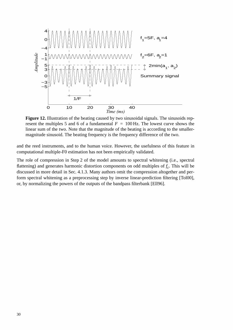
and the reed instruments, and to the human voice. However, the usefulness of this feature incomputational multiple-F0 estimation has not been empirically validated.
The role of compression in Step 2 of the model amounts to spectral whitening (i.e., spectralflattening) and generates harmonic distortion components on odd multiples of fc. This will bediscussed in more detail in Sec. 4.1.3. Many authors omit the compression altogether and per-form spectral whitening as a preprocessing step by inverse linear-prediction filtering [Tol00],or, by normalizing the powers of the outputs of the bandpass filterbank [Ell96].
0 10 20 30 40
−5−3
0
3 5
−1 1
−4
0
4
f1=5F, a
1=4
f2=6F, a
2=1
Summary signal
2min(a1, a
2)
1/F
Figure 12. Illustration of the beating caused by two sinusoidal signals. The sinusoids rep-resent the multiples 5 and 6 of a fundamental Hz. The lowest curve shows thelinear sum of the two. Note that the magnitude of the beating is according to the smaller-magnitude sinusoid. The beating frequency is the frequency difference of the two.
F 100=
Time (ms)
Am
plitu
de
30

4 Auditory-model based multiple-F0 estimator
The aim of this chapter is to investigate how the principles of the unitary pitch model (intro-duced in Sec. 3.5) can be utilized in practical multiple-F0 estimation. A novel method is pro-posed which estimates the F0s of several concurrent musical sounds in a single time frame.Computational efficiency of the method is based on the algorithm proposed in [P4]. Accuracyof the method is based on specific modifications to the unitary model which are originally pro-posed here.
In Sec. 4.1, a detailed frequency-domain analysis of the unitary pitch model is presented. Thisserves as background material for [P4] and paves the way for the algorithm presented in it. InSec. 4.2, the auditory-model based multiple-F0 estimator is presented. The method is based onthe analysis of the unitary model in Sec. 4.1.
Throughout this chapter it should be kept in mind that our aim is not to propose a model of thehuman auditory system (this issue was discussed in Sec. 1.3.1). The approximations and modi-fications to be proposed to the unitary model are ultimately justified by the fact that, as a result,a practically applicable multiple-F0 estimation algorithm is obtained.
4.1 Analysis of the unitary pitch model in frequency domain
The summary autocorrelation function (SACF) of the unitary pitch model has turned out to bea very useful mid-level representation (see Sec. 1.2.3) in several tasks, such as multiple-F0estimation, sound separation, and computational auditory scene analysis [deC99, Tol00,Wan99, Ell95,96, Ros98a]. However, the computational complexity of calculating the SACF israther high, due to the ACF calculations at 40–128 subbands (the number varies in differentimplementations). This has limited the usability of the model in practical applications.
In [P4], we have proposed a method for calculating an approximation of the SACF in the fre-quency domain. Concretely, what the algorithm achieves is to compute one spectral line of theFourier transform of the SACF, , in O(K) time, given the complex Fourier spec-trum of the input sound. Here K is the length of the transform frame and the order-of-growthnotation O(•) is according to the common usage [Cor90]. The individual spectral lines allowcomputationally efficient multiple-F0 estimation as will be described in Sec. 4.2.
Another thing achieved by the algorithm in [P4] is that it removes the need to define thenumber of distinct subbands. The algorithm implements a model where one subband is cen-tered on each discrete Fourier spectrum sample, thus approaching a continuous density of sub-bands. The bandwidths of the channels need not be changed. This is exactly the opposite to theapproach of Tolonen et al. in [Tol00], where a computationally efficient version of the unitarypitch model was proposed by reducing the number of subbands to two. Tolonen’s multiple-F0estimation method is rather successful and has been evaluated in [P5].
The presentation in [P4] is very condensed due to the page limit. In the following, backgroundmaterial that facilitates the understanding of [P4] is presented. A starting point for the algo-rithm is to perform the four calculation phases of SACF (see Sec. 3.5) in the frequencydomain. This inevitably leads to frame-based processing. However, this is not a serious prob-lem, since the ACF calculations involved in the conventional SACF calculations are in practicealways performed on a frame-by-frame basis to allow FFT-based ACF computations ([Ell96]represents an exception).
DFT st τ( )( )
4 AUDITORY-MODEL BASED MULTIPLE-F0 ESTIMATOR 31

In the following, we look at the processing steps of the unitary pitch model in more detail. Par-ticular emphasis is laid on the first two steps of the unitary model: (i) the bank of bandpass fil-ters and (ii) compression, rectification, and lowpass filtering at the subbands. As alreadymentioned in the previous chapter, performing the mentioned nonlinear operations at specificsubbands leads to a number of attractive properties from the point of view of multple-F0 esti-mation. Thus, the two steps are studied in depth. Time-domain compression, which was notdiscussed in [P4], is included here.
4.1.1 Auditory filters (Step 1 of the unitary model)
The cochlea is an organ in the inner ear which transforms sound pressure level variations intoneural impulses in the auditory nerve. Frequency analysis is an essential part of this process.Frequency components of a complex sound can be perceived separately and are coded inde-pendently in the auditory nerve (in distinct nerve fibers), provided that their frequency separa-tion is sufficiently large [Moo95b]. The auditory frequency analyzer is usually modeled as abank of overlapping, linear, bandpass filters, called auditory filters. Combination of informa-tion across channels then takes place in the central nervous system.
The concept critical band is closely related to the auditory filters. The term was coined byFletcher in 1940 [Fle40]. Fletcher’s experiment is illustrated in Figure 13a. He measured thethreshold of detecting a sinusoidal signal in the presence of a bandpass noise masker whichwas centered on the signal frequency. The power spectral density of the noise was held con-stant but the noise bandwidth was varied. Detection threshold increased as a function of thenoise bandwidth, but only up to a certain point. Fletcher labeled this bandwidth a “criticalband” and suggested that the frequency analysis of the inner ear could be modeled with a bankof bandpass filters (which became to be called auditory filters). Noise components contibute tomasking in proportion to their power at the output of the filter which captures the target signal.
Even later, the auditory filters have been most often studied using the masking phenomenon.Masking refers to a situation where an audible sound becomes inaudible in the presence ofanother, louder sound. In particular, if the distance of two spectral components is less than thecritical bandwidth, one easily masks the other. The situation can be thought of as if the compo-nents would go to the same auditory filter, to the same “channel” in auditory nerve. If the fre-quency separation is larger, the components are coded separately and are both audible.
By making certain assumptions about the auditory filters, it is possible to measure the band-width and the shape of their power response. The notched-noise method as originally sug-gested by Patterson in [Pat76] is illustrated in Fig. 13b. A wide-band noise signal with aspectral notch (a stopband) is used to mask a sinusoidal tone. The notch is centered on the tone,and the threshold of detecting the sinusoid as a function of the width of the notch is measured.Two main assumptions are made. First, that the auditory filter which captures the sinusoidalsignal is centered on the signal frequency and is reasonably symmetric on a linear frequencyscale, and secondly, that masking is due to the part of noise which leaks to the same auditorychannel at the sides. Because the detection threshold level is known be directly proportional tothe masking noise level [Pat86], the amount of noise leaking to the channel and thus the shapeof the auditory filter can be deduced. By placing noise bands on both sides it can be ensuredthat the signal is not heard through the neighbouring auditory filters, i.e., by “off-frequency lis-tening”.
32

The shape of the auditory filters has been approximated with simple mathematical expressionsthat have few free parameters. Patterson et al. have suggested three different formulas [Pat86].It is convenient to express the formulas in terms of a new frequency variable
, (4.1)
where normalization with the center frequency facilitates the comparison of filters with dif-ferent center frequencies. As can be seen, measures normalized deviation from the centerfrequency. The squared magnitude response of the rounded exponential, roex, filter as sug-gested in [Pat86] is given by
(4.2)where p is a parameter which determines the bandwidth of the filter. The response is illustratedin Fig. 14. Other models have been proposed, too, but only at the expense of more parametersfor the magnitude response function. In the unitary model, the exact shape of the auditory filterresponse is not critical, therefore it does not make sense to look at the more complex functions.The model in (4.2) is completely sufficient for our purposes and has spread to wide use, largelybecause the response can be implemented computationally efficiently using gammatone filters[Sla93].
The bandwidths of auditory filters can be conveniently expressed using the equivalent rectan-gular bandwidth (ERB) concept. The ERB of a filter is defined as the bandwidth of a perfectrectangular filter which has a unity response in its passband and integral over the squared mag-nitude response which is the same as for the specified filter. Integral over the squared roexresponse is obtained by substituting (4.1) to (4.2), integrating over the right half of theresponse, and multiplying the result by two:
600 800 1000 1200 14000
0.5
1
Noise NoiseSignal
Notch bandwidth
600 800 1000 1200 14000
0.5
1
1.5
2
Noise bandwidth
Signal level
Figure 13. (a) Illustration of Fletcher’s experiment. See text for details. (b) Idea of thenotched-noise method which has been used to determine the shape of the auditory filterresponse (after [Pat76]). In both panels, the power spectral density of the noise is constantand signal level is varied.
Frequency (Hz)
Pow
er
Pow
er
Frequency (Hz)
(a) (b)
gf f c–
f c---------------=
f cg
Ψ roex( ) g( ) 1 p g+( )e p g–=
−0.4 −0.2 0 0.2 0.40
0.5
1
−0.6 −0.4 −0.2 0 0.2 0.4 0.6−40
−20
0
Figure 14. Squared magnitude response of the rounded-exponential (roex) filter.
Relative frequency g Relative frequency g
Ψg()
[dB
]Ψ
g()
4 AUDITORY-MODEL BASED MULTIPLE-F0 ESTIMATOR 33

. (4.3)
Glasberg and Moore measured the ERB values of the auditory filters over a wide range ofcenter frequencies using the notched noise method [Gla90]. They found that the ERB valuescan be described as a linear function of the center frequency as
, (4.4)
where the center frequency and the bandwidth are in hertz units. In the following, we use theshorthand notation to refer to the ERB value of an auditory filter according to (4.4), andto refer to the corresponding center frequency of the filter.
By setting the ERB values in (4.3) and (4.4) equal, the variable p of the roex filters can be cal-culated as
. (4.5)
As a result, the response of a roex filter at a given center frequency is fully determined.
The center frequencies of the filters in the auditory filterbank are typically assumed to be uni-formly distributed on a critical-band scale. This frequency-related scale is derived by integrat-ing the inverse of (4.4) which yields
. (4.6)
In the above expression, f is frequency in hertz and gives the critical-band scale. Intui-tively, this means that the auditory filters are more densely distributed at the low frequencieswhere the ERB values are smaller. More exactly, the power responses of the filters sum to a flatresponse over the whole range of center frequencies. When f varies between 20Hz and 20kHz(the hearing range), varies between 0.8 and 42. Intuitively, this means that approximately41 critical bands (auditory filters) would fit to the range of hearing if the passbands of the audi-tory filters were non-overlapping and rectangular in shape.
4.1.2 Flatted exponential filters
The algorithm in [P4] has been derived for a certain family of filters called flatted-exponential,flex, filters. The shape of the response of these filters differs somewhat from that of rounded-exponential filters. From the point of view of the unitary pitch model, however, the exact shapeof the response is not critical, but the important characteristics of the auditory filters are thatthey are approximately uniformly distributed on the critical band scale given by (4.6), that thebandwidths are according to (4.4), and that the number of filters is large enough to make thepassbands of adjacent filters overlap significantly.
Three requirements suffice to fully define the response of the flatted-exponential filters. (i) Thefilters implement a flat (unity) response around the center frequency of the filter. (ii) The slopeof attenuation further away from the center frequency is defined to be the same as the asymp-totic attenuation of the rounded-exponential filters. The attenuation of the roex filters followsthe slope further away from the center frequency, since the factor in (4.2)becomes insignificant for large values of . (iii) The ERB value of the filters is defined to bethe same as that of the corresponding roex filter, i.e., according to (4.4).
2 Ψ roex( ) f( ) fd
f c
∞
∫ 2 1 p f f c–( ) f c⁄+( )e p f f c–( ) f c⁄–[ ] fd
f c
∞
∫4 f c
p---------= =
u f c( ) 24.7 1 4.37 f c 1000⁄+[ ]=
uc f c
p4 f c
uc---------=
e f( ) 21.4log10 4.37 f 1000⁄ 1+( )=
e f( )
e f( )
e p g– 1 p g+( )g
34

The flatted-exponential filter response is illustrated in Fig. 15 and can be written as
(4.7)
where the frequency variable g is as defined in (4.1) and the variable stems fromthe requirement (ii) above.
The parameter g0, i.e., the half-width of the flatted top can be determined by requiring that theERB-bandwidths of flex and roex filters must be equal for a given parameter p:
(4.8)
Integral over the squared flex response is obtained by integrating piecewise over the right halfand multiplying by two. The above equation becomes
(4.9)
and by integrating
(4.10)
from which we obtain . The flex filter in (4.7) can now be written as
(4.11)
In terms of frequency variable f this becomes (simply substitute p from (4.5) and g from (4.1)):
. (4.12)
Please note that (4.12) gives the squared magnitude response of the flex filter. In the following,we use the shorthand notation for the above power response and
to refer to the corresponding discrete magnitude response of a flex filter at center fre-quency fc and with the ERB bandwidth uc according to (4.4). That is, a bank of flatted-expo-nential bandpass filters will be applied in the unitary-model in the following.
−0.4 −0.2 0 0.2 0.40
0.5
1
−0.6 −0.4 −0.2 0 0.2 0.4 0.6−40
−20
0
Figure 15. Solid line shows the squared magnitude response of the flatted-exponential(flex) filter. Dashed line shows the response of the rounded-exponential (roex) filter
Relative frequency g Relative frequency g
Ψg() [d
B]
Ψg()
Ψ flex( ) g( )1
p– g g0–( )[ ]exp
=g g0≤
g g0>
p 4 f c uc⁄=
Ψ flex( ) g( ) gd
∞–
∞
∫ Ψ roex( ) g( ) gd
∞–
∞
∫=
2 1 gd
0
g0
∫ 2 p– g g0–( )[ ]exp[ ] gd
g0
∞
∫+ 2 1 pg+( )e pg– gd
0
∞
∫=
2g02p---+ 4
p---=
g0 1 p⁄=
Ψ flex( ) g( )1
p– g 1+( )exp
=g 1 p⁄≤g 1 p⁄>
Ψ flex( ) f c f,( )1
4 f f c– uc⁄– 1+[ ]exp
=f f c– uc 4⁄≤
f f c– uc 4⁄>
Ψhcf( ) Ψ flex( ) f c f,( )∼
Hc k( )
4 AUDITORY-MODEL BASED MULTIPLE-F0 ESTIMATOR 35

4.1.3 Compression and half-wave rectification at subbands (Step 2 of the unitary model)
In the unitary pitch model as originally described in [Med91a,b], the output of each auditoryfilter was processed by a hair-cell model. In human hearing, when a sound enters the inner ear,it travels as a pressure wave within the cochlea. Hair cells are the elements which transform theresulting mechanical movement to neural impulses. The hair-cell model used in [Med91a,b]was a dynamic system described in terms of differential equations [Med86]. However, as laterpointed out by the authors, the hair cells in the unitary pitch model can equally well be mod-eled as a cascade of compression, half-wave rectification, and lowpass filtering [Med97] (seealso [Med91a], p. 2869). This approach is followed here. In some previous implementations,the compression has been omitted (see e.g. [Ell96, Tol00]). This can be done if the task of thecompression is carried out by some other means of preprocessing.
In the following, compression and half-wave rectification are each discussed separately. Theseare thought of as a cascade, where full-wave vth-law compression is performed first and this isfollowed by rectification.
Full-wave (odd) vth-law compression (FWOC) is defined to have the transfer characteristic
, (4.13)
where v > 0. This specific form of compression is employed here because it matches suffi-ciently well the measured compression in hair cells (see [Med86]) and because it is analyti-cally tractable and numerically safe.
What happens in the frequency domain when a narrowband signal is compressed as above? Asa nonlinear operation, FWOC of course does not have a “frequency response”. However, con-sider a narrowband input , where is the center fre-quency of the spectral band and . Here “narrowband” means that the bandwidth of
is small compared to . This, in turn, implies that the variations of and areslow compared to those of . For such a signal, the output of a full-wave vth-lawcompressor can be expressed as [Dav87]
, (4.14)
where the coefficient is
, (4.15)
and is the Gamma function. That is, the output of the vth-law compressor consists of asignal at the frequency of the input narrowband signal and at the odd multiples of it. The enve-lope of each of these is modulated by the vth-power of the input envelope and the mth harmonicis phase-modulated by m times the input phase modulation.
The expression in (4.14) applies reasonably accurately for the subband signals at the outputs ofthe auditory filterbank. The subband signals are sufficiently narrowband to satisfy the assump-tions for all except few lowest channels. That is, the subband signals can be imagined as having
FWOC x( )xv x 0≥
x–( )v– x 0<
=
x t( ) A t( ) ωct φ t( )+( )cos= f c ωc 2π⁄=A t( ) 0≥
x t( ) f c A t( ) φ t( )ωct( )cos y t( )
y t( ) 2C v m,( ) A t( )[ ] v mωct mφ t( )+[ ]cosm 1=
m odd( )
∞
∑=
C v m,( )
C v m,( ) Γ v 1+( )
2vΓ 1 m v–2
-------------– Γ 1 m v+
2-------------+
----------------------------------------------------------------------=
Γ x( )
36

been modulated to their center frequencies. We denote by the time-domain signal at theoutput of an auditory filter centered on frequency . The discrete Fourier transform of thissignal is denoted by
(4.16)
and the discrete Fourier transform of the vth-law compressed signal is denoted by
. (4.17)
At the passband of the auditory filter, the Fourier spectrum of the compressed signal can beapproximated as
, when . (4.18)
Here is a scalar, K is the transform length, and is the sampling rate. The approximationgets less accurate when v gets very small ( ) or large ( ) values but, for moderatecompression levels used here ( ), the approximation is sufficiently accurate. Thescaling factor can be calculated from (4.14) as
, (4.19)
where is the standard deviation of the subband signal and is the amplitude of a vir-tual “carrier” sinusoidal signal which has the standard deviation . The approximation in(4.18)–(4.19) can be straightforwardly verified experimentally.
At the passband of the auditory filter, the scaling factor in (4.19) tends to normalize the stand-ard deviation of the subband signal towards unity when . In this sense, the compressioncan be omitted if the sound spectrum is appropriately preprocessed (whitened) before the audi-tory filterbank. This has been done e.g. in [Tol00]. Ellis, in turn, took the approach of normal-izing the outputs of the auditory filters by their energies [Ell96, p.77]. The distortion spectrumat odd multiples of could be accurately modeled, too, but this will not be done in the fol-lowing. At moderate compression levels, the magnitude of these is small compared to the pass-band of the auditory filter and, furthermore, the subsequent lowpass filter eliminates much ofthe distortion spectrum. Thus it is seen as not having an important role in the unitary pitchmodel.
In the following, the scaling of subbands according to (4.18) is seen purely and simply as apsychoacoustically inspired way of performing spectral whitening. The fact that the model wasderived from time-domain vth-law compression is not so important. The presented form ofspectral whitening is convenient because it provides a single parameter with which to deter-mine the degree of applied whitening. Also, interestingly, when v in (4.19) gets very small val-ues, the spectrum due to scaling with at subbands does not approach a white spectrum, butrather, a pink spectrum. This is because the standard deviations are measured at criticalbands which are approximately logarithmically spaced and have bandwidths which are linearlyproportional to the center frequency. For these reasons, spectral whitening according to (4.18)is considered to be advantageous over e.g. inverse linear-prediction filtering.
The non-linear half-wave rectification (HWR) operation, as defined in (3.5), is a core part ofthe unitary model. In [Dav87] it has been shown that for an input zero-mean gaussian randomprocess , an approximate expression for the power spectral density of the output
of the half-wave rectifier can be written as
xc n( )f c
Xc k( ) DFT xc n( )[ ]=
Xccomp( ) k( ) DFT xc n( )v[ ]=
Xccomp( ) k( ) γcXc k( )≈ k f s K⁄ f c– uc<
γc f sv 0.3< v 3>
0.3 v 1< <γc
γc 2C v 1,( ) σc 2( ) v 1–( )=
σc σc 2σc
v 1<
f c
γcσc
x t( ) Ψy f( )y t( ) HWR x t( )( )=
4 AUDITORY-MODEL BASED MULTIPLE-F0 ESTIMATOR 37

, (4.20)
where is the power spectral density of the input and is the unit impulse function.The approximation involved in the above expression is that higher-order convolution termshave been omitted due to their small powers. As shown in [Dav87], this leads to an error in theoutput variance which is less than 3%.
Figure 16 illustrates the magnitude spectrum of the output of the half-wave rectifier in the casethat the input process has a narrow-band rectangular spectrum. (It should be noted that (4.20)does not assume a narrowband signal although these are of interest here.) For a narrowbandsignal xc(n) centered on fc, the output spectrum consists of a dc-component, of the originalpower spectrum scaled down by four, and of a convolution of the original power spectrum byitself which produces spectral components centered on zero-frequency and twice the inputcenter frequency. In principle, HWR generates spectral components also to bands centered onall integer multiples of fc without upper limit, but the other bands are very small in power[Dav87].
In the unitary pitch model, phases play an important role and therefore the approximationderived for the power spectral densities in (4.20) is not sufficient. In terms of complex-valueddiscrete Fourier spectra, the approximation becomes the following1. Let
(4.21)
be the short-time Fourier transform of time-domain signal before rectification and
(4.22)
be the short-time Fourier transform of the rectified time-domain signal. We use todenote an approximation of the spectrum . The approximation becomes
, (4.23)
where is the standard deviation of the time-domain signal before rectification2.
In the present context, the signals of interest are composed of a limited number of sinusoidal
1. Deriving these approximations is rather straightforward, although not trivial, based on the standardanalyses in [Dav87]. An interested reader is referred to Chapter 12 in the cited book.
Ψy f( )σx
2
2π------δ f( ) 1
4---Ψx f( ) 1
4πσx2
------------- Ψx f ′( )Ψx f f ′–( ) f ′d
∞–
∞
∫+ +≈
Ψx f( ) δ f( )
B
2B
−2fc
−fc −B B f
c2f
c
dc−component
Figure 16. Power spectrum of a half-wave rectified narrowband signal which is centeredon frequency fc and has a bandwidth B (after [Dav87]).
X k( ) x n( )e i2π n 1–( )k– K⁄n 1=
K∑=
x n( )
W k( ) HWR x n( )[ ] e i2π n 1–( )k– K⁄n 1=
K∑=
W k( )W k( )
W k( )σx
8π----------δ k( ) 1
2---X k( ) 1
σx 8π----------------- X l( )X k l–( )
l K 2⁄– k+=
K 2⁄ k–
∑+ +=
σx x n( )
38

components and do not satisfy the gaussianity assumption very well. Despite that, the approxi-mation in (4.23) turned out to be quite accurate, as can be easily verified experimentally. Cer-tain complications arise, however, if the time-domain signal is windowed prior to therectification. This is because time-domain windowing violates the stationarity assumption ofthe model. The problem can be easily circumvented by performing windowing as a convolu-tion in the frequency domain after computing . That is, is convolved with the Fou-rier spectrum of the window function. (In the time domain, this is achieved simply by applyingwindowing as usual when computing the term in (4.23) but using the square rootof the window function to obtain which is used in the place of for the convolutionterm in (4.23). These technical details are relatively unimportant from the point of view of theanalysis here.)
Let be the time-domain signal at the output of an auditory filter centered on frequency. According to (4.23), the complex spectrum of after rectification can be approxi-
mated by
, (4.24)
where we have denoted the convolution term
(4.25)
for convenience. An unbiased estimate of the standard deviation of is obtained basedon as
, (4.26)
since gives the power of the signal at channel c.
Spectral whitening according to (4.18)–(4.19) can be included by writing
, (4.27)
where the scaling factors at different channels can be calculated by substituting to(4.19). Weighting the last term by the square of stems from the definition of in(4.25).
After compression and half-wave rectification, the subband signals are lowpass filtered, asmentioned in the beginning of this subsection. Traditionally, a fixed lowpass filter isused for all different channels and, in addition, the dc-component of the subband signals isremoved. More exactly, the filter typically implements a bandpass response with a -3dB cutofffrequencies around 60Hz and 1.0kHz. As a consequence, the dc-term in (4.27) can be omittedand the spectrum at the output of channel c can be expressed as
2. At first, the convolution terms in (4.20) and (4.23) may appear as contradictory. However, it has to beremembered that these are merely approximations. The latter approximation is more precise among thetwo.
x n( )
W k( ) W k( )
1 2⁄( )X k( )X' k( ) X k( )
xc n( )f c xc n( )
W c k( )σc
8π----------δ k( ) 1
2---Xc k( ) 1
σc 8π-----------------V c k( )+ +=
V c k( ) Xc l( )Xc k l–( )l K 2⁄– k+=
K 2⁄ k–
∑=
σc xc n( )V c k( )
σc V c 0( ) K 1–( )⁄=
V c 0( ) xc n( )
W c k( )γcσc
8π-----------δ k( )
γc
2-----Xc k( )
γc2
σc 8π-----------------V c k( )+ +=
γc σcγc V c k( )
HLP k( )
4 AUDITORY-MODEL BASED MULTIPLE-F0 ESTIMATOR 39

. (4.28)
4.1.4 Periodicity estimation and across-channel summing (Steps 3 and 4 of the unitarymodel)
The autocorrelation function (ACF) is equal to the inverse Fourier transform of the power spec-trum. Thus the Fourier transform of the autocorrelation function rc(τ) at subband c isobtained as
. (4.29)
In practice, the spectra and are non-overlapping at all except few lowest chan-
nels and (4.29) can be approximated by
. (4.30)
This approximation is valid at channels above about 150Hz but, since we are not interested inreproducing all the nuances and artefacts of the unitary pitch model, we use it at all channels.Also, from the point of view of harmonic sounds, the lowest channels usually do not containmore than one significant frequency component, in which case the magnitude of is verysmall for (see (4.25)).
Summary autocorrelation function s(τ) is calculated by summing the within-channel ACF esti-mates as given by (3.6). Since Fourier transform and its inverse are linear operations, we cansum already in the frequency domain to obtain the Fourier transform of s(τ),
(4.31)
and then perform a single inverse Fourier transform to obtain the summary autocorrelation
function s(τ).
Using the approximation in (4.30), the two terms can be squared and summed separately. It fol-
lows that (4.31) can be approximated by
. (4.32)
The bandpass filters are typically designed so that their power responses sum to unity, as men-tioned around (4.6). In this case and, because is slowly-varying asa function of c, the above formula can be written as
, (4.33)
where is the compression-modeling scaling factor corresponding to the frequency bin k. Agood approximation of is obtained by computing the standard deviation of the subband sig-nal at the band centered on the frequency bin k and by substituting this value to (4.19)1. Thealgorithm presented in [P4] computes in time for all channels c with center fre-
HLP k( )W c k( ) HLP k( )γc
2-----Xc k( )
γc2
σc 8π-----------------V c k( )+
=
Rc k( )
Rc k( ) HLP k( )γc
2-----Xc k( )
γc2
σc 8π-----------------V c k( )+
2
=
Xc k( ) V c k( )
Rcˆ k( ) HLP k( )
γc
2-----X
ck( )
2HLP k( )
γc2
σc 8π-----------------V c k( )
2
+=
V c k( )k 0≠
Rc k( )
S k( ) Rc k( )c∑=
S k( ) HLP k( ) 2γc
2-----Xc k( )
2
c∑ HLP k( ) 2γc
2
σc 8π-----------------V c k( )
2
c∑+=
Xc k( ) 2c∑ X k( ) 2= γc
S k( ) HLP k( ) 2γk
2-----X k( )
2HLP k( ) 2
γc2
σc 8π-----------------V c k( )
2
c∑+=
γkγk
V c 0( ) O K( )
40

quencies , thus the standard deviations needed to compute arein practice really available. The spectra do not need to be calculated at all.
In the discussion to follow, it will be convenient to denote
, (4.34)
, (4.35)
and to express in two parts as
. (4.36)
Note that is the whitened power spectrum of the input wideband signal.
Finally, the inverse Fourier transform is used to obtain an approximation of the summaryautocorrelation function as
. (4.37)Because IDFT is a linear operation, also can be decomposed into two terms as
, (4.38)
where
, (4.39)
. (4.40)
As described around Fig. 10 on page 25, the IDFT performs implicit pattern matching on thepower spectrum. In (4.39), pattern matching is performed on harmonic locations of the (whit-ened) power spectrum of the input wide-band signal, similarly to the conventionalACF (see Fig. 10). In (4.40), pattern matching is performed on which is the across-chan-nel sum of the power spectra of the amplitude envelopes of the subband signals. The envelopespectra contain frequency components which correspond to the frequency intervals in the orig-inal spectrum. This was described in Sec. 3.5.1 and is explicitly visible in the definition of
in (4.25).
Thus the two types of information, spectral-location information ( ) and spectral-intervalinformation ( ) can be kept (approximately) separate until the very end, and can be accu-mulated separately across bands.
The summary autocorrelation function value represents the weight of a period candidate, or, the strength of the pitch sensation for pitch period candidate . The lag corresponding to
the maximum of is typically considered as the pitch period.
In the above discussion, has been referred to as the amplitude-envelope spectrum at
subband c. In addition to that, however, contains the distortion spectrum centered on
frequency , and the IDFT operation in (4.40) collects frequency components from both
bands. Figure 17 shows an example of the power spectrum for an artificial subchan-
1. In principle, should be computed as a weighted average of several in the vicinity of k but inpractice the difference is negligible.
γk γc
f c 1 2 … K 2⁄, , ,( ) f s K⁄= γkXc k( )
X k( )γk
2-----X k( )
2=
V k( )γc
2
σc 8π-----------------V c k( )
2
c∑=
S k( )
S k( ) HLP k( ) 2 X k( ) V k( )+( )=
X k( )
s τ( )
s τ( ) IDFT S k( )( )=s τ( )
s τ( ) s1 τ( ) s2 τ( )+=
s1 τ( ) IDFT HLP k( ) 2X k( )( )=
s2 τ( ) IDFT HLP k( ) 2V k( )( )=
X k( ) 2
V k( )
V c k( )
s1 τ( )s2 τ( )
s τ( )τ τ
s τ( )
V c k( )V c k( )
2 f cV c k( ) 2
4 AUDITORY-MODEL BASED MULTIPLE-F0 ESTIMATOR 41

nel signal, the power spectrum of which is shown in the left panel.
There are reasons to believe that the distortion spectrum centered on does not play any
significant role in the unitary model and therefore does not deserve a more detailed analysis.
First, the lowpass filter attenuates the distortion spectrum at channels for which
Hz. As will be described in Sec. 4.2, these higher channels are the most important for
the envelope-related term because their bandwidth is wider and they typically contain
more dense sets of frequency partials. Secondly, the channels below 500Hz contain only har-
monic partials whose harmonic index h (see (3.1)) is small ( even for low-pitched
sounds). For these partials, significant inharmonicity is not observed, and therefore the spec-
trum centered on consists of frequency components at ideal harmonic position as in
Fig. 17. In this case, the IDFT pattern-matcher picks the generated spectral peaks both around
zero frequency and around , and the role of the distortion spectrum on is merely quan-
titative: to emphasize the information which is already represented by the band around zero
frequency. The situation would be more complicated if significant inharmonicity would be
observed at the lower channels because, in this case, the peaks around would not occur at
harmonic locations and IDFT would not “match”.
4.1.5 Algorithm proposed in [P4]
Publication [P4] is concerned with the term which consists of the sum of the envelopespectra at different channels as seen in (4.35). Each spectrum , in turn, is calcu-lated by convolving the subband spectrum with itself according to (4.25). Thus, it iseasy to see that calculating is computationally demanding for a large number of sub-bands.
The algorithm proposed in [P4] computes for a fixed k and for all channels c with centerfrequencies in a time which is linearly proportional to K (trans-from length), when given the wideband Fourier spectrum as input. This means that eachfrequency bin in can be computed in O(K) time, given the spectrum . As mentionedin the beginning of this chapter, this has consequences which lead to a computationally effi-cient unitary-model based F0 estimator.
The basic idea of the algorithm described in [P4] is to compute an estimate of orbased on in constant time (O(1)), with few arithmetic operations. Thus we
only need to initialize for or and then iteratively calculate for
−1200 −800 −400 0 400 800 12000
0.5
1
1.5
f1
f∆
Frequency (Hz)
Pow
er
−1200 −800 −400 0 400 800 12000
0.05
0.1
f∆f∆2 f
1
Frequency (Hz)
Po
we
r
Figure 17. Left: Power spectrum of an artificial subband signal with 100Hz fun-damental frequency. Center frequency of the auditory filter is fc=500Hz and, for simplic-ity, a rectangular response is used as the auditory filter. Right: Power spectrum(defined in (4.25)) corresponding to the power spectrum on the left.
Xc k( ) 2
V c n( ) 2
2 f c
HLP k( )f c 500>
s2 τ( )
1 h 10≤ ≤
2 f c
2 f c 2 f c
2 f c
V k( )V c k( ) V c k( )
Xc k( )V k( )
V c k( )f c 1 2 … K 2⁄, , ,( ) f s K⁄=
X k( )V k( ) X k( )
V c 1+ k( )V c 1– k( ) V c k( )
V c k( ) c 1= c K 2⁄= V c k( )
42

all channels c by using the update rules proposed in [P4]. As a results, we obtain one spectralline of . The update rules were given for the family of flatted-exponential, flex, filters butsimilar rules could be derived for any filter with a magnitude response which is piecewise rep-resentable with exponential functions ( ) as is the case with the flex filter in(4.12).
As a starting point for deriving the update rules, is decomposed as
(4.41)
where is the response of the flex filter centered at fc. Now (4.25) can be written as
. (4.42)
In the above equation, the convolution spectrum for a given k,
(4.43)
is common to all c. This is filtered with a varying convolved response
. (4.44)
As illustrated in Figure 18, the convolved response can be of two basic types, depending onwhether the flatted tops of the two flex responses overlap or not. However, both types consist offive parts (A–E in Fig. 18) which are of the form of an exponential function .The update rules proposed in [P4] are based on this observation. Imagine that we have com-puted the value of for a certain channel c in (4.42) and that the sum over each of the fiveparts of the convolved response are separately known. Take part A as an example. Sum overthis part in the neighbouring channel c+1 is obtained by “shifting” the part A upwards in thespectrum and integrating over that part. The integral for c+1 is directly obtained by multiplyingthe sum in channel c with a constant (smaller than one) which causes the old values graduallyleak out from the sum and by adding new spectral components when they come under the inte-gral. This way the sum can be updated iteratively over the whole spectrum. More detailed for-mulas for computing estimates of or based on are given in [P4].Important in doing this is that the iterative calculations are performed so that numerical errors
V k( )
α1 α2 f α3+( )exp
Xc k( )
Xc k( ) Hc k( )X k( )=
Hc k( )
V c k( ) Hc l( )X l( )Hc k l–( )X k l–( )l K 2⁄– k+=
K 2⁄ k–
∑=
Zk l( ) X l( )X k l–( )=
Jc k, l( ) Hc l( )Hc k l–( )=
350 400 450 500 5500
0.5
1A B C D EType II
350 400 450 500 5500
0.5
1
A B C D E
Type I
Figure 18. The thick curves in the two panels illustrate the two basic types of the con-volved response given by (4.44). The two responses and areshown with dotted and dashed lines, respectively.
Jc k, l( ) Hc l( ) Hc k l–( )
Frequency (Hz)
Frequency (Hz)
Mag
nitu
deM
agni
tude
α1 α2 f α3+( )exp
V c k( )
V c 1+ k( ) V c 1– k( ) V c k( )
4 AUDITORY-MODEL BASED MULTIPLE-F0 ESTIMATOR 43

do not cumulate in the calculations.
The computations briefly introduced above lead to a linear distribution of subband center fre-quencies where the center frequency of channel c is . The desired channel distri-bution, however, is uniform on the critical-band scale defined in (4.6). This problem is easilycircumvented. An arbitrary distribution of center frequencies can be simulated by weightingthe outputs of the linearly-distributed channels accordingly. This is possible when the channeldensity is sufficiently high, as is the case here. A uniform distribution of channels on the criti-cal-band scale can be simulated by weighting the outputs of the linearly-distributed channelsby where the bandwidth is computed according to (4.4).
The spectrum at each channel c consists of two frequency bands, one centered on zerofrequency and another centered on . These two have to be computed separately using thealgorithm described in [P4]. However, only the calculations of the band centered on zero fre-quency were described in [P4] and the band centered on was ignored. This was not veryclearly stated in [P4] and is therefore mentioned in the errata of [P4] on page 111. The bandcentered on could be computed exactly in the same way (simply changing in(4.43)), but since we are interested only in the spectrum of the amplitude envelope centered onzero frequency, this is not presented in more detail. For convenience in the following, wedenote
, (4.45)
where is an ideal lowpass filter with cutoff frequency and zero-valued phaseresponse. That is, contains only the amplitude envelope spectrum centered on zero fre-quency and not the distortion spectrum centered on .
4.2 Auditory-model based multiple-F0 estimator
In this section, the above-presented analysis is applied in order to obtain a practically applica-ble multiple-F0 estimation tool for use in music signals. The method is based on using thewhitened wide-band spectrum in (4.34) and the amplitude envelope spectra in(4.45). The main difference compared to the unitary model is that the ACF calculations in(4.39)–(4.40) (IDFT of the power spectrum) are replaced by a more suitable technique. In thepresent context, practical F0-estimation accuracy is what counts.
The human auditory system is very good at multiple-F0 estimation. The unitary pitch model, inturn, successfully simulates many of the qualitative properties of human pitch perception, sug-gesting that the model works in a way similar to its physiological counterpart. Nothing wouldbe more natural than to pursue accurate multiple-F0 estimation by recruiting the unitary model.This has been attempted by us for monophonic signals in [Kla99a] and later for polyphonicmixtures (unpublished). Other authors have reported work to this direction in [Mar96b, deC99,Tol00, Wu02]. However, it has turned out that the unitary model as such is not a very accuratemultiple-F0 estimator.
In the following, we analyze why the unitary model often fails in practical multiple-F0 estima-tion tasks. Then, a few modifications are proposed to remove these shortcomings. An overviewof the modifications will be given in Sec. 4.2.2. Before that, the backgrounding signal modeland the concept resolvability will be introduced in the next subsection. Sections 4.2.3–4.2.5will discuss the proposed modifications in detail. Computational efficiency will be consideredin Sec. 4.2.6. Extending a single-F0 estimator to the multiple-F0 case is described in
f c c f s K⁄=
1 uc⁄ uc
V c k( )2 f c
2 f c
2 f c Zk l( )
V c ′ k( ) HLP f c( ) k( )V c k( )=
HLP f c( ) k( ) f cV c ′ k( )
2 f c
X k( ) V c ′ k( )
44
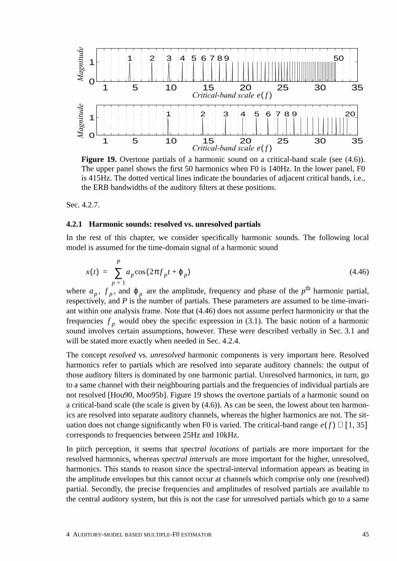
Sec. 4.2.7.
4.2.1 Harmonic sounds: resolved vs. unresolved partials
In the rest of this chapter, we consider specifically harmonic sounds. The following localmodel is assumed for the time-domain signal of a harmonic sound
(4.46)
where , , and are the amplitude, frequency and phase of the pth harmonic partial,respectively, and P is the number of partials. These parameters are assumed to be time-invari-ant within one analysis frame. Note that (4.46) does not assume perfect harmonicity or that thefrequencies would obey the specific expression in (3.1). The basic notion of a harmonicsound involves certain assumptions, however. These were described verbally in Sec. 3.1 andwill be stated more exactly when needed in Sec. 4.2.4.
The concept resolved vs. unresolved harmonic components is very important here. Resolvedharmonics refer to partials which are resolved into separate auditory channels: the output ofthose auditory filters is dominated by one harmonic partial. Unresolved harmonics, in turn, goto a same channel with their neighbouring partials and the frequencies of individual partials arenot resolved [Hou90, Moo95b]. Figure 19 shows the overtone partials of a harmonic sound ona critical-band scale (the scale is given by (4.6)). As can be seen, the lowest about ten harmon-ics are resolved into separate auditory channels, whereas the higher harmonics are not. The sit-uation does not change significantly when F0 is varied. The critical-band rangecorresponds to frequencies between 25Hz and 10kHz.
In pitch perception, it seems that spectral locations of partials are more important for theresolved harmonics, whereas spectral intervals are more important for the higher, unresolved,harmonics. This stands to reason since the spectral-interval information appears as beating inthe amplitude envelopes but this cannot occur at channels which comprise only one (resolved)partial. Secondly, the precise frequencies and amplitudes of resolved partials are available tothe central auditory system, but this is not the case for unresolved partials which go to a same
x t( ) ap 2πf pt ϕ p+( )cosp 1=
P
∑=
ap f p ϕ p
f p
1 5 10 15 20 25 30 350
1 1 2 3 4 5 6 7 8 9 50
1 5 10 15 20 25 30 350
1 1 2 3 4 5 6 7 8 9 20
Critical-band scale e f( )
Mag
nitu
de
Figure 19. Overtone partials of a harmonic sound on a critical-band scale (see (4.6)).The upper panel shows the first 50 harmonics when F0 is 140Hz. In the lower panel, F0is 415Hz. The dotted vertical lines indicate the boundaries of adjacent critical bands, i.e.,the ERB bandwidths of the auditory filters at these positions.
Mag
nitu
de
Critical-band scale e f( )
e f( ) 1 35,[ ]∈
4 AUDITORY-MODEL BASED MULTIPLE-F0 ESTIMATOR 45

channel with their neighbouring harmonics.
Also simple psychoacoustic experiments support the view that spectral-location information ismore important for the low-order (resolved) partials. For example, the pitch of a harmonicsound does not change significantly if its even-numbered harmonics are removed. However, ifthe odd-numbered harmonics are removed, the pitch doubles because the remaining harmonicscorrespond to those of a two-times higher sound. This suggests that the spectral locationsaffect the perception of pitch. However, this is not the case when only higher-order harmonicsare involved: the spectral intervals dominate and it becomes impossible to say whether aneven-numbered or an odd-numbered series of harmonics is higher in pitch. In [Kla99b], wecarried out a small psychoacoustic experiment to determine the limit, up to which the humanauditory system discerns the spectral locations of harmonic partials. A total of nine subjectswere presented with a pair of harmonic sounds, one composed of a set of five successive odd-numbered harmonics, and another of a set of five successive even-numbered harmonics. Thesubjects were asked which one of the sounds was higher in pitch. In cases where the series ofpartials was among the lower harmonics, the subjects perceived a clear octave difference. Inthe higher end, however, the octave difference disappeared and the subjects selected odd/evenseries to be higher with 50% probability. I.e., the spectral-location dependency disappeared. Inall cases, the F0 of the sound was 137Hz and the order of presentation was randomized.
In the unitary model, the terms and correspond to spectral-location and spectral-interval information, respectively. Based on the above discussion, we make the important inter-pretation that the term represents mainly the resolved harmonics and the term rep-resents mainly the unresolved harmonics. This interpretation is maintained throughout theanalysis in the previous section so that also the terms and in (4.24)–(4.33) areinterpreted to be oriented towards resolved and unresolved partials, respectively. The mostobvious argument for this is the fact that amplitude envelope beating at the F0 rate, or, signifi-cant components in , occur only when several partials go to a same auditory channelwhich is the case for the unresolved harmonics. Finally, in (4.39) is interpreted to repre-sent mainly the resolved partials and in (4.40) mainly the unresolved partials.
4.2.2 Overview of the proposed modifications
The modifications to be proposed in the following are directed at the steps 3 and 4 of the uni-tary model. The ACF calculations are replaced by a technique called harmonic selection andmore complex subband-weighting is applied when combining the results across bands. Asdescribed in Sec. 3.5, the steps 3–4 of the unitary model are a matter of dispute in psychoa-coustics and, from the point of view of practical F0-estimation, the attractive properties of theunitary model stem from the steps 1 and 2.
Harmonic selection is here defined as the principle that only a set of selected spectral compo-nents are used when computing the “salience” of a F0 candidate, instead of using the overallspectrum. The word salience is here used to refer to the calculated weight, or, likelihood, of aF0 candidate. The word “likelihood” is not used because it carries a probabilistic connotationwhich is not given to the word salience. In multiple-F0 estimation, it is desirable to minimizethe interference of other co-occurring sounds and, therefore, it is more robust to use only thepartials of a hypothesized F0 candidate to compute its salience and to ignore the spectrumbetween the partials. In cases where several F0s are present, usage of the overall spectrum isproblematic since the salience calculations get confused by the co-occurring sounds and inter-
X k( ) V k( )
X k( ) V k( )
Xc k( ) V c k( )
V c k( )s1 τ( )
s2 τ( )
46

relations of different sounds cause unpredictable combination-effects. The general principle ofharmonic selection was originally proposed by Parsons in [Par76] and a comprehensive reviewof the previous harmonic selection and harmonic cancellation methods can be found in[deC93].
In the time domain, harmonic selection can be implemented by using a bank of comb filtersand by measuring the energies at the outputs of the filters. Each comb filter is characterized bya certain feedback delay and a feedback gain . The output of a comb filterwith feedback delay can be written as
. (4.47)
Figure 20 illustrates the power response of a comb filter with corresponding to 100Hz and. For comparison, the weights of the ACF calculation are shown for the same delay,
analogous to Fig. 10 on page 25. Estimating the energy of the output can be performedby squaring and summing in the time domain which is equivalent to summing over the powerspectrum of the filtered signal.
We implement harmonic selection (i.e., a comb-filter like response) directly in the frequencydomain. For the resolved harmonics, a frequency bin to represent the harmonic partial p of afundamental frequency candidate is selected from the spectrum as
, (4.48)
where
, (4.49)
, (4.50)
. (4.51)
Above, defines a range in the vicinity of the ideal harmonic frequency where themaximum of is assumed to indicate the partial p. The scalar represents spacingbetween successive period estimates . Here, we use a constant sampling of lag values,
, analogous to the ACF. The set is defined so that, for a fixed partial index p, allspectral components belong to the range of at least one candidate , and the ranges ofadjacent period candidates and cannot overlap by more than one frequency bin.
The selected frequency bins are used to compute a salience function whichreplaces in (4.38). The function represents the contribution of resolved harmonics
τ 0 α 1< < yτ n( )τ
yτ n( ) 1 α–( )x n( ) α yτ n τ–( )+=
0 100 200 300 400 500 600 700
−1
0
1
0 100 200 300 400 500 600 700 0
1
Frequency (Hz)Frequency (Hz)
Wei
ght
Pow
er r
espo
nse
Figure 20. Left panel shows the weights of ACF calculation in (3.3) whenthe lag corresponds to 100Hz (i.e., lag is 10ms). Right panel shows the power response ofa comb filter with a feedback delay corresponding to 100Hz and feedback gain 0.85.
2πτk K⁄( )cosτ
τα 0.85=
yτ n( )
F f s τ⁄=
k p τ, marg axk K p τ,∈
X k( )( )=
K p τ, k p τ,0( ) … k p τ,
1( ), ,[ ]=
k p τ,0( ) pK τ ∆τ 2⁄+( )⁄ 1+=
k p τ,1( ) max pK τ ∆τ 2⁄–( )⁄ k p τ,
0( ),{ }=
K p τ, pK τ⁄X k( ) ∆τ
τ∆τ 1= K p τ,
K p τ, ττ τ ∆τ+
k p τ, λ1 τ( )s1 τ( ) λ1 τ( )
4 AUDITORY-MODEL BASED MULTIPLE-F0 ESTIMATOR 47

to the salience of a period candidate . The function is computed as
, (4.52)
where the two-parameter function determines the weights of different harmonics inthe sum and, as a side-effect, determines the upper limit up to which the partials are consideredas “resolved” and thus included in the sum (i.e., the weight approaches zero for large p). Thesum cannot be extended to arbitrarily large values of p because only the lower-order harmonicscan be expected to reside at approximately harmonic positions of the spectrum. As will be seenin the next subsection, the “degree of resolvability” of a partial, , is a two-parameterfunction, depending on the frequency of the partial p and the fundamental frequency .
Applying the weights in (4.52) represents another fundamental departure from theunitary model. It should be noted that the summing in (4.52) occurs across auditory channels.This is because resolved harmonics, by definition, are located at distinct channels. In hearing,the resolved harmonics are separately coded in the auditory nerve and it is the task of the cen-tral auditory system to recombine this information so that the partials of a harmonic sound areperceived as a coherent whole. Thus it is conceivable that some more complex weighting cantake place for the resolved harmonics in pitch calculations.
For comparison, let us write out the salience function which is being replaced by :
. (4.53)
Above, a unity weight is assigned to partials at harmonic positions of the spectrum and, pro-vided that there are partials at these locations, their powers are summed with unity weights upto the cutoff frequency of the lowpass filter . This is not very suitable as such1.
There is a lot of evidence that pitch perception for harmonic sounds resembles a spectral pat-tern-matching process, especially for the lower-order partials which are resolved into separateauditory channels [Gol73, Wig73, Ter74,82a,b, Har96]. However, the process is not likely totake the form of lowpass filtering followed by ACF calculation but happens in a more complexmanner in the central nervous system.
The salience function in (4.52) is based on the assumption that the frequencies andamplitudes of individual resolved partials are available to the central auditory system whichprocesses those parameters whatever way it wishes. There is no particular necessity to stick tothe ACF. It is important to note that the lowpass filter in (4.53) and the weight func-tion in (4.52) model two different things. The filter models the response ofthe hair-cells which transform mechanical vibration into neural impulses in the inner ear. Theweights , in turn, model a pattern-matching process which is assumed to take place in
1. Consider a low-pitched sound with F0 100Hz. In polyphonic music, the frequency range between100Hz and 1.0kHz is heavily occupied by other sounds. Blindly picking components from all harmonicpositions and weighting them equally is not robust. The implicit spectral smoothing mechanismdescribed in Sec. 3.5.3 would partly prevent from “stealing” the partials of other sounds, but this mech-anism is involved only in the amplitude-envelope related part . For a high-pitched sound with F01.0kHz, in turn, the lowest and most important harmonic partials are each resolved to separate auditorychannels. As such, they cannot generate beating frequencies to and, in (4.53), they are rejectedby the lowpass filter. In practice, F0s above about 600Hz are detected very poorly.
τ
λ1 τ( ) w p τ,( ) X k p τ,( )[ ]p∑=
w p τ,( )
w p τ,( )f s τ⁄
w p τ,( )
s1 τ( ) λ1 τ( )
s1 τ( ) 1K---- 2πτk
K------------ cos HLP k( ) 2X k( )
k 0=
K 1–
∑=
HLP k( )
V k( )
V c k( )
λ1 τ( )
HLP k( )w p τ,( ) HLP k( )
w p τ,( )
48

the central nervous system. In principle, the filter should be included in (4.52) (thehair-cell response cannot be bypassed), but since acts as a lowpass filter, canbe omitted.
Another, less important modification is that, in (4.52), magnitude spectrum is used instead ofthe power spectrum in (4.53). This modification is due to both simplicity and accuracy. Thesecond power stems from the ACF computations and there is no particular reason to maintainit. On the contrary, as discussed below (3.2), it is usually advantageous to use a “generalizedACF” where the exponent is below two. Tolonen and Karjalainen suggest the value 0.67 in[Tol00]. This is a matter of fine-tuning and not important here, therefore the unity value is usedfor simplicity.
The other part, in (4.38), represents mainly the unresolved harmonics as discussed inthe previous subsection. This is replaced by a salience function where harmonic selec-tion is applied in a manner analogous to that described above. The salience function isdefined as
, (4.54)
where is a real-valued constant and is obtained by substituting in (4.49). First,note that magnitude spectra at different channels c are used, instead of the power spectra as in(4.35). This modification is due to the same reasons as for the part. Also, as defined in(4.45), contains only the amplitude-envelope spectrum centered on zero frequency andnot the distortion spectrum centered on . Secondly, only one frequency bin is selected inthe vicinity of the fundamental frequency . This can be computed very efficiently usingthe algorithm in [P4] and leads to a very efficient overall implementation as will be describedin Sec. 4.2.6.
Individual frequency bins at each channel c suffice to represent the salience contribu-tion of unresolved harmonics for the fundamental frequency candidate . Acomplete argument for this is given in Sec. 4.2.4 but an intuitive description is given here. Notethat the single frequency bin retains all the desirable properties of the unitary pitchmodel described in Sec. 3.5. First, represents spectral-interval oriented informationregarding the fundamental frequency . The magnitude of reveals theamount of amplitude-envelope beating at rate at subband c. The beating, in turn, is due to allfrequency components with interval at channel c. If the fundamental frequency F is present,each two neighbouring harmonics contribute to the beating at the rate F, and the magnitude of
is high. Secondly, due to the manner how the amplitude of the beating is formed (seeFig. 12 on page 30), retains the property of implicit spectral smoothing. Thirdly,
is phase-dependent because it is computed using the complex Fourier spectrum,according to (4.25) and (4.45). If the harmonics of a sound are phase-locked to each other (lin-ear phase, i.e., the phase difference between each pair of neighbouring harmonics is approxi-mately constant), the magnitude of the beating at the fundamental rate is larger.
The overall salience of a period candidate is then defined (analogously to (4.38)) as:
. (4.55)
The maximum of is used to indicate the fundamental period. The corresponding funda-mental frequency is . This represents one detected F0 in a mixture signal. An exten-
HLP k( )w p τ,( ) HLP k( )
s2 τ( )λ2 τ( )
λ2 τ( )
λ2 τ( ) maxk K1 τ,∈
η0HLP k( )γc
2
σc 8π-----------------V c ′ k( )
c∑
=
η0 K1 τ, p 1=
λ1 τ( )V c ′ k( )
2 f cK τ⁄
V c ′ k0( )F k0 K⁄( ) f s=
V c ′ k0( )V c ′ k0( )
F k0 K⁄( ) f s= V c ′ k0( )F
F
V c ′ k0( )V c ′ k0( )
V c ′ k0( )
τ
λ τ( ) λ1 τ( ) λ2 τ( )+=
λ τ( )F f s τ⁄=
4 AUDITORY-MODEL BASED MULTIPLE-F0 ESTIMATOR 49

sion to multiple-F0 estimation will be described in Sec. 4.2.7.
4.2.3 Degree of resolvability
This subsection is concerned with the coefficient in (4.52). The coefficient was inter-preted as the degree of resolvability for harmonic p of fundamental period candidate . Thesalience function was calculated by selecting frequency components nearby harmonicspectral locations, by weighting their magnitudes by , and by summing these. Weight-ing different partials p by their resolvability is motivated by the fact that the spectral locationsof partials are important only in the case of resolved partials, as discussed in Sec. 4.2.1.
The boundary between resolved and unresolved partials is not sharp but we have to speakabout “degree of resolvability”. How could this be measured? For the overtone partials of aharmonic sound, resolvability depends on the F0 and on the harmonic index p of the partial.This can be seen by estimating the number of partials which go to a same auditory channeltogether with harmonic number p. The frequency interval between partials is determined quiteaccurately by the the fundamental frequency F, and the ERB bandwidth of the auditory chan-nel around harmonic p can be estimated by substituting to (4.4). The ratio of thesecan be used to estimate the number of partials going to a same auditory channel withharmonic p:
. (4.56)
As can be seen, grows linearly as a function of the harmonic index p. (Note that theabove simple ratio gets values below unity when the inter-partial interval is larger than theERB value.)
We propose to model the degree of resolvability as proportional to the inverse of :
, (4.57)
where the scalar is an unknown parameter that has to be experimentally found. Apart fromsaying that represents the degree of resolvability, the function is not given any exactpsychoacoustic interpretation. It has merely practical use. Note that the above ratio (excluding
) gets values above unity for the few lowest harmonics, meaning that some auditory chan-nels around those partials do not contain partials at all. Although the neighbouring channelsactually should not affect the resolvability, for simplicity, the measure in (4.57) is used in thefollowing without limiting the maximum value of the above ratio to a unity value.
The function controls the contribution of partial p to the salience function .Figure 21 illustrates the values of for the first 20 harmonics of a few fundamental fre-quency values. As can be seen, the contribution of partial p to the salience functiondecreases as a function of the harmonic index p. Here, more or less arbitrarily, we use
.
It is interesting to note that the contribution of an overtone partial p to the other salience func-tion, , increases as a function of p. This occurs although no weighting function is explic-itly included in (4.54). As described around (4.54), a single frequency bin is selectedto represent the salience contribution of unresolved harmonics to the fundamental frequencycandidate at channel c. According to the decomposition in (4.42),
w p τ,( )
w p τ,( )τ
λ1 τ( )w p τ,( )
f c pF=ϒ p F,( )
ϒ p F,( ) 24.7 1 4.37 pF 1000⁄+[ ]F
-----------------------------------------------------------=
ϒ p F,( )
ϒ p F,( )
w p F,( ) w0F
24.7 1 4.37 pF 1000⁄+[ ]-----------------------------------------------------------=
w0w p F,( )
w0
w p F,( ) λ1 τ( )w p F,( )
λ1 τ( )
w0 0.5=
λ2 τ( )V c ′ k0( )
F k0 K⁄( ) f s= V c ′ k0( )
50

can be calculated by summing over l in , where is the convolution spec-trum and is the convolved response at channel c. For a fixed fundamental frequencycorresponding to , the term remains the same at different channels. However, theterm varies along with the channel index c. As can be seen inFigure 18, if is small compared to the bandwidth of , the passbands of and
overlap a lot in the convolution and the overall power transmission of the con-volved response is high. Because the bandwidth increases linearly as a function of thecenter frequency (see (4.4)), the power transmission of increases with frequency. Thishas the consequence that the contribution of the harmonic series of a sound to the saliencefunction increases as a function of the harmonic index p. On the other hand, for a fixedsubband c, the power response of decreases with an increasing (increasing funda-mental frequency).
Based on the above description, we can express the average spectral density of theconvolved response at channel centered on and for fundamental frequency F as
, (4.58)
where is the frequency bin corresponding to . Note that the denominatorrepresents the ERB value (i.e., bandwidth) of the flex response at channel c. Normalizationwith the bandwidth is important in order to compensates for the effect which is merely due tothe fact that the ERB values increase with frequency. That is, the average spectral density ofthe convolved response, not the overall power transmission, acts as the weight for individualharmonic partials that reside at that particular channel.
The value represents an implicit weight which affects the salience contribution of anovertone partial p to the function . Figure 22 illustrates for the first 20 harmon-ics of a few fundamental frequency values. The curves have been obtained by substituting
in (4.58). As can be seen, the salience contribution increases monothonically withharmonic index p and saturates to unity. As a consequence, the function indeed repre-sents mainly the unresolved partials. No upper limit for the harmonic index needs to be set. Inpractice, however, significant harmonic components are not observed above 6–8kHz and itdoes not make sense to consider subbands with center frequencies above this.
It seems reasonable that the functions and would sum approximately to
1 5 10 15 200
1
2
3
4
Figure 21. Values of for the first 20 harmonic overtones of a few F0 values. Thecurves (bottom-up) correspond to F0 values 70Hz, 150Hz, 300Hz, and 1.0kHz, respec-tively. The applied value of the scalar is 0.5.
w p F,( )
w0
Harmonic index hW
eigh
t
Zk0l( )Jc k0, l( ) Zk0
l( )Jc k0, l( )
k0 Zk0l( )
Jc k0, l( ) Hc l( )Hc k0 l–( )=k0 Hc l( ) Hc l( )
Hc k0 l–( )Jc k0, l( )
Jc k0, l( )
λ2 τ( )Jc k0, l( ) k0
ξ f c F,( )Jc k, l( ) f c
ξ f c F,( )Jc kF, l( )
l∑Jc 0, l( )
l∑---------------------------
Hc l( )Hc kF l–( )l∑
Hc l( )Hc l–( )l∑
------------------------------------------------= =
kF F f s⁄( )K= F
ξ pF F,( )λ2 τ( ) ξ f c F,( )
f c pF=λ2 τ( )
w p F,( ) ξ pF F,( )
4 AUDITORY-MODEL BASED MULTIPLE-F0 ESTIMATOR 51

unity over the harmonic series of a sound, so that the harmonics which contribute only little tothe salience function would contribute more to the salience function , implement-ing a smooth transition between the resolved and unresolved partials.
The thin solid line in Fig. 23 illustrates the degree of resolvability (with )as a function of the harmonic index p. Along with that, the dashed line shows as afunction of p. The sum of the two is drawn with a thicker line. As can be seen, the two func-tions sum approximately to unity over the harmonic series of a sound. For the lowest few har-monics of high-pitched sounds, however, the sum clearly exceeds the unity value. This isbecause the modeled resolvability in (4.57) was not limited to values below unity.However, the additional boost for the few lowest harmonics of high-pitched sounds turned outto be a good feature, since the high-pitched sounds typically have only few harmonic compo-nents altogether, and the boost compensates for this.
Table 3 shows the pseudocode of the algorithm which computes the salience function .The algorithm has several nice properties. First, it is not computationally very complex, since itis safe to consider only the first 20 harmonics of each period candidate due to the fact that theweight becomes quite small above this. When the partial index p is fixed, the numberof elements in the sets for different altogether is less than ,where is the number of period candidates and K is the transform length. Thus, the overallcomplexity of the algorithm is of the order when a fixednumber of 20 partials is considered. Secondly, only the selected frequency components affectthe salience of a F0 candidate, not the overall spectrum. This provides some robustness in
1 2 4 6 8 10 12 14 16 18 200
0.2
0.4
0.6
0.8
1
norm
aliz
ed p
ower
harmonic index
Figure 22. The function for the first 20 harmonic overtones of a few F0 values.The function reflects the contribution of the harmonics to the salience function . Thecurves (top-down) correspond to F0 values 70Hz, 150Hz, 300Hz, and 1.0kHz, respectively.
ξ pF F,( )λ2 τ( )
λ1 τ( ) λ2 τ( )
1 5 10 15 200
0.5
1
1.5
weig
ht
harmonic index1 5 10 15 20
0
0.5
1
1.5
2
weig
ht
harmonic index1 5 10 15 20
0
1
2
3w
eig
ht
harmonic index1 5 10 15 20
0
1
2
3
4
weig
ht
harmonic index
Figure 23. Thin solid line shows (with ) as a function of the harmonicindex p. Dashed line shows . The sum of the two functions is indicated by thicksolid line. F0 values are 70Hz, 150Hz, 300Hz, and 1.0kHz, from left to right, respectively.
w p F,( ) w0 0.5=ξ pF F,( )
w p F,( ) w0 0.5=ξ pF F,( )
w p F,( )
λ1 τ( )
w p F,( )k 0( ) … k 1( ), ,[ ] τ T∈ K T+
TO 20 K T+( )( ) O K T+( )=
52
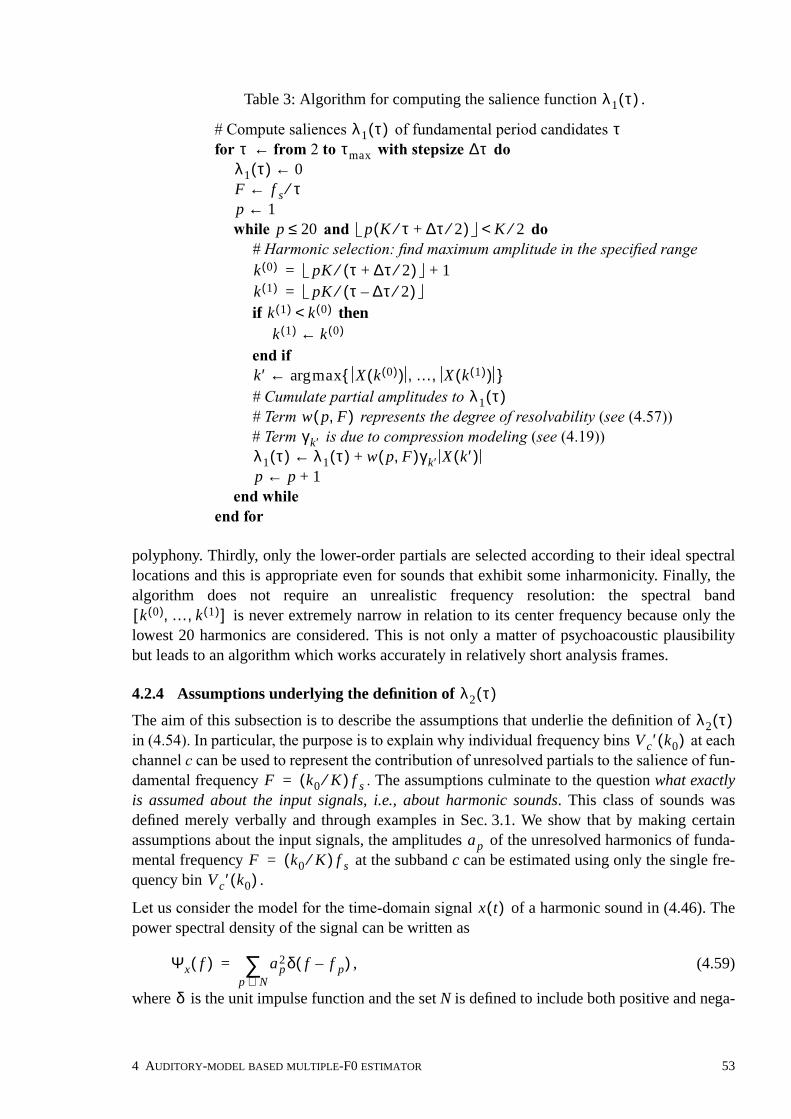
polyphony. Thirdly, only the lower-order partials are selected according to their ideal spectrallocations and this is appropriate even for sounds that exhibit some inharmonicity. Finally, thealgorithm does not require an unrealistic frequency resolution: the spectral band
is never extremely narrow in relation to its center frequency because only thelowest 20 harmonics are considered. This is not only a matter of psychoacoustic plausibilitybut leads to an algorithm which works accurately in relatively short analysis frames.
4.2.4 Assumptions underlying the definition of
The aim of this subsection is to describe the assumptions that underlie the definition ofin (4.54). In particular, the purpose is to explain why individual frequency bins at each
channel c can be used to represent the contribution of unresolved partials to the salience of fun-
damental frequency . The assumptions culminate to the question what exactlyis assumed about the input signals, i.e., about harmonic sounds. This class of sounds wasdefined merely verbally and through examples in Sec. 3.1. We show that by making certainassumptions about the input signals, the amplitudes of the unresolved harmonics of funda-mental frequency at the subband c can be estimated using only the single fre-quency bin .
Let us consider the model for the time-domain signal of a harmonic sound in (4.46). Thepower spectral density of the signal can be written as
, (4.59)
where is the unit impulse function and the set N is defined to include both positive and nega-
# Compute saliences of fundamental period candidates
for ← from 2 to with stepsize do
while and do# Harmonic selection: find maximum amplitude in the specified range
if then
end if
# Cumulate partial amplitudes to# Term represents the degree of resolvability (see (4.57))
# Term is due to compression modeling (see (4.19))
end whileend for
λ1 τ( ) ττ τmax ∆τλ1 τ( ) 0←F f s τ⁄←p 1←
p 20≤ p K τ⁄ ∆τ 2⁄+( ) K 2⁄<
k 0( ) pK τ ∆τ 2⁄+( )⁄ 1+=k 1( ) pK τ ∆τ 2⁄–( )⁄=
k 1( ) k 0( )<k 1( ) k 0( )←
k ′ marg ax X k 0( )( ) … X k 1( )( ), ,{ }←λ1 τ( )
w p F,( )γk ′
λ1 τ( ) λ1 τ( ) w p F,( )γk ′ X k ′( )+←p p 1+←
Table 3: Algorithm for computing the salience function .λ1 τ( )
k 0( ) … k 1( ), ,[ ]
λ2 τ( )
λ2 τ( )V c ′ k0( )
F k0 K⁄( ) f s=
apF k0 K⁄( ) f s=
V c ′ k0( )
x t( )
Ψx f( ) ap2δ f f p–( )
p N∈∑=
δ
4 AUDITORY-MODEL BASED MULTIPLE-F0 ESTIMATOR 53

tive indexes, . Negative indexes are used to express negative frequen-cies, i.e., and for .
When the signal is passed through a critical-band auditory filter with a squared magnituderesponse as defined in (4.12), the output of the filter can be denoted by
. Using the signal model in (4.59), this can be written as
. (4.60)
When half-wave rectification is applied on the subband signal , the power spectral den-sity of the resulting rectified signal can be approximated using (4.20) as
(4.61)
where is the variance of the subband signal .
We denote the convolution term1 in the above expression by :
. (4.62)
Examples of the power spectra and were illustrated in Fig. 17 on page 42.
The first necessary assumption concerning the input harmonic sounds is that the frequencyinterval between adjacent harmonics, , remains approximately constantwithin one critical band. This assumption is reasonable for the kind of inharmonicity that weconsider in this work (dispersive strings etc.). Even when sounds exhibit inharmonicity, thespectral intervals are slowly-varying as a function of frequency (see e.g. (3.1)) and can beassumed to be piecewise constant at sufficiently narrow bands. Using this assumption, the sin-gle spectral line at subband c can be calculated as
, (4.63)
when is constant at the subband c.
Secondly, we know that for the higher-order unresolved harmonics, the human auditory systemdoes not distinguish the amplitudes of individual harmonic components. Instead, the roughspectral shape of several components is perceived (approximately one level measure per a crit-ical band and a distinct sound source). If one harmonic raises clearly above the other partials, itis usually perceptually segregated and stands out as an independent sound. This feature ofhearing is well modeled by the unitary pitch model as discussed in Sec. 3.5.
In the computational analysis of sounds, it is useful to make a “spectral smoothness” assump-tion similar to that in human hearing. More specifically, we assume that the partial amplitudes
within one critical band c centered on frequency fc can be approximated by a single level
1. Due to the differences in the two approximations (4.20) and (4.23), is not the exact power
spectrum of as defined in (4.25). Instead, is an approximation. For this reason, the
notation is used instead of .
N P 1–,–[ ] 1 P,[ ]∪=f p– f p–= a p– ap= n N∈
x t( )Ψhc
f( )Ψxc
f( ) Ψx f( )Ψhcf( )=
Ψxcf( ) ap
2δ f f p–( )Ψhcf p( )
p N∈∑=
xc t( )yc t( )
Ψycf( )
σc2
2π------δ f( ) 1
4--- ap
2δ f f p–( )Ψhcf p( )
p N∈∑
14πσc
2------------- δ f f i– f j+( )ai
2a j2Ψhc
f i( )Ψhcf j( )
j N∈∑
i N∈∑
+
+
=
σc2 xc t( )
Ψvcf( )
Ψvcf( )
V c k( ) Ψvcf( )
Ψvcf( ) Ψvc
f( )
Ψvcf( ) 1
4πσc2
------------- δ f f i– f j+( )ai2a j
2Ψhcf i( )Ψhc
f j( )j N∈∑
i N∈∑=
Ψxcf( ) Ψvc
f( )
f ∆ f p 1+ f p–=
Ψvcf ∆( )
Ψvcf ∆( ) 2
4πσc2
------------- ap2 ap 1+
2 Ψhcf p( )Ψhc
f p 1+( )p 1=
P 1–
∑=
f ∆ f p 1+ f p–=
ap
54
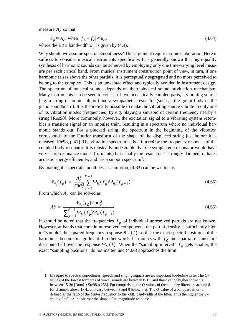
measure so that
, when , (4.64)
where the ERB bandwidth is given by (4.4).
Why should we assume spectral smoothness? This argument requires some elaboration. Here itsuffices to consider musical instruments specifically. It is generally known that high-qualitysynthesis of harmonic sounds can be achieved by employing only one time-varying level meas-ure per each critical band. From musical instrument construction point of view, in turn, if oneharmonic raises above the other partials, it is perceptually segregated and no more perceived tobelong to the complex. This is an unwanted effect and typically avoided in instrument design.The spectrum of musical sounds depends on their physical sound production mechanism.Many instruments can be seen to consist of two acoustically coupled parts, a vibrating source(e.g. a string or an air column) and a sympathetic resonator (such as the guitar body or thepiano soundboard). It is theoretically possible to make the vibrating source vibrate in only oneof its vibration modes (frequencies) by e.g. playing a sinusoid of certain frequency nearby astring [Ros90]. More commonly, however, the excitation signal to a vibrating system resem-bles a transient signal or an impulse train, resulting in a spectrum where no individual har-monic stands out. For a plucked string, the spectrum in the beginning of the vibrationcorresponds to the Fourier transform of the shape of the displaced string just before it isreleased [Fle98, p.41]. The vibration spectrum is then filtered by the frequency response of thecoupled body resonator. It is musically undesirable that the symphatetic resonator would havevery sharp resonance modes (formants) but usually the resonator is strongly damped, radiatesacoustic energy efficiently, and has a smooth spectrum1.
By making the spectral smoothness assumption, (4.63) can be written as
(4.65)
From which can be solved as
. (4.66)
It should be noted that the frequencies of individual unresolved partials are not known.However, at bands that contain unresolved components, the partial density is sufficiently highto “sample” the squared frequency response so that the exact spectral positions of theharmonics become insignificant. In other words, harmonics with inter-partial distance aredistributed all over the response . When the “sampling interval” gets smaller, theexact “sampling positions” do not matter, and (4.66) approaches the limit
1. In regard to spectral smoothness, speech and singing signals are an important borderline case. The Q-values of the lowest formants of vowel sounds are between 8-15, and those of the higher formantsbetween 15-30 [Dun61; Ste98,p.258]. For comparison, the Q-values of the auditory filters are around 8for channels above 1kHz and vary between 3 and 8 below that. The Q-value of a bandpass filter isdefined as the ratio of the center frequency to the -3dB bandwidth of the filter. Thus the higher the Q-value of a filter, the sharper the shape of its magnitude response.
Ac
ap Ac≈ f p f c– uc<uc
Ψvcf ∆( )
Ac4
2πσc2
------------- Ψhcf p( )Ψhc
f p 1+( )p 1=
P 1–
∑=
Ac
Ac4
Ψvcf ∆( )2πσc
2
Ψhcf p( )Ψhc
f p 1+( )p 1=
P 1–∑-----------------------------------------------------------------=
f p
Ψhcf( )
f ∆Ψhc
f( ) f ∆
4 AUDITORY-MODEL BASED MULTIPLE-F0 ESTIMATOR 55
. (4.67)
Here, the frequencies of the individual partials need not be known.
In conclusion, the single frequency bin suffices to represent the level of the partials offundamental frequency at subband c. Of course, this result depends on thevalidity of the above assumptions and of the approximation for a half-wave rectified signalgiven by (4.20). Virtanen and Klapuri used the described assumptions and (4.20) to estimatethe parameters of the unresolved harmonic components in a sound separation system (unpub-lished at the present time). In resynthesis, good perceptual quality was achieved for the higher-order unresolved partials using the described model and assumptions.
Provided that an input sound indeed has sinusoidal partials with constant intervals at chan-nel c, it is easy to see that the convolution term contains partials also at the multiples
, where integer . However, it is not necessary to extend the harmonicselection so that also these components would be picked from and summed. In fact, theamplitudes given by (4.67) can be used to predict (approximate) the magnitudes of thespectral lines , for as:
(4.68)
Substituting from (4.67) this can be written as
. (4.69)
Let us see what difference it would make to select and sum up all the harmonically related par-tials , where . The sum would be
. (4.70)
The sum on the right-hand side of the above equation merely amounts to a very complicatedweighting of the individual spectrum line . Such weighting turned out to be com-pletely unnecessary.
The purpose of the above analysis was to motivate the use of only one frequency binat each channel c to represent the contribution of unresolved partials to the salience of funda-mental frequency candidate at those channels. As already discussed inSec. 4.2.2, the single frequency bin retains the desirable properties of the unitary pitchmodel.
For convenience, let us rewrite here the definition of from (4.54):
Ac4
Ψvcf ∆( )2πσc
2
1f ∆------ Ψhc
f( )Ψhcf f ∆+( ) fd
f∫-------------------------------------------------------------------≈
Ψvcf ∆( )
F k0 K⁄( ) f s=
f ∆Ψvc
m f ∆ m 1 2 3 …, , ,=Ψvc
AcΨvc
m f ∆( ) m 1>
Ψvcmf ∆( )
Ac4
2πσc2
------------- Ψhcf p( )Ψhc
f p m+( )p 1=
P m–
∑Ac
4
2πσc2
------------- 1f ∆------ Ψhc
f( )Ψhcf m f ∆+( ) fd
f∫≈
=
Ac4
Ψvcmf ∆( ) Ψvc
f ∆( )Ψhc
f( )Ψhcf m f ∆+( ) fd
f∫Ψhc
f( )Ψhcf f ∆+( ) fd
f∫-----------------------------------------------------------------≈
Ψvcmf ∆( ) m 1 2 3 …, , ,=
Ψvcmf ∆( )
m∑ Ψvc
f ∆( )Ψhc
f( )Ψhcf m f ∆+( ) fd
f∫Ψhc
f( )Ψhcf f ∆+( ) fd
f∫-----------------------------------------------------------------
m∑≈
Ψvcf ∆( )
V c ′ k0( )
F k0 K⁄( ) f s=V c ′ k0( )
λ2 τ( )
56

. (4.71)
Note that in the above equation, the values are used directly and are not used to esti-mate the magnitudes of the individual partials according to (4.67). Using the magni-tudes of the partials, , would omit the implicit “weighting” of individual harmonics by
as described in the previous subsection and in Figs. 22–23. This would not be appro-priate since , by definition, should represent mainly the unresolved harmonics. This, inturn, is because was interpreted to represent mainly the unresolved harmonics.
The filter in (4.71) cannot be omitted. As described in the end of Sec. 4.1.3, the recti-fied signal contains a significant dc-component and, in order to remove this, the filtertypically implements a bandpass response with -3dB cutoffs around 60Hz and 1kHz. Since weare using instead of , only the highpass characteristics of the filter are important.(The term contains only the amplitude-envelope spectrum centered on zero frequencyand not the distortion spectrum centered on .) Figure 24 illustrates the frequency responseof the applied butterworth filter of order four per each transition band and with the -3dB cutoffat 60Hz. The scaling factor in (4.71) is a free parameter which will be determined in thenext subsection.
4.2.5 Model parameters
The overall salience of different fundamental period candidates is given by (4.55). A niceproperty of the overall model is that it contains only few free parameters. However, an impor-tant parameter which remains to be determined is the relative weight of the two partsand . Note that both parts include an unknown scaling factor: for in (4.57) and
for in (4.54). The numerical ranges of the two parts have to be matched in order thatboth terms would have an appropriate effect on . It suffices to balance the levels ofand in relation to each other since the absolute numerical range of is not impor-tant. Thus, for simplicity, we fix and consider only as a free parameter.
Another important parameter is the value v of the vth-law compression in (4.19). Thirdly, thewidths of the subbands were found to be an important tunable parameter in the model. Weapplied a scalar so that the used bandwidths were , where is according to (4.4). Inother words, the factor scales the defined critical bandwidths and this has an effect everywherewhere these bandwidths are used, without having to modify the other parts.
The parameters , v, and were found experimentally in simulations. Musical instrumentsamples were randomized from an acoustic database and the accuracy of the F0 estimation
λ2 τ( ) maxk K1 τ,∈
η0HLP k( )γc
2
σc 8π-----------------V c ′ k( )
c∑
=
V c ′ k( )ap Ac≈
apξ pF F,( )
λ2 τ( )V c ′ k( )
HLP k( )HLP k( )
V c ′ k( ) V c k( )V c ′ k( )
2 f c
0 20 40 60 80 100 120 1400
0.2
0.4
0.6
0.8
1
Frequency (Hz)
Mag
nitu
deFigure 24. Magnitude response of the filter applied on in (4.71). Due tothe narrowband nature of , characteristics of the filter above 1kHz are not important.
HLP k( ) V c ′ k( )V c ′ k( )
η0
λ τ( )
λ1 τ( )λ2 τ( ) w0 λ1 τ( )
η0 λ2 τ( )λ τ( ) λ1 τ( )
λ2 τ( ) λ τ( )η0 1= w0
ucu0 u0uc uc
w0 u0
4 AUDITORY-MODEL BASED MULTIPLE-F0 ESTIMATOR 57

method for this material was evaluated using different parameter values. The database com-prised a total of 2536 individual recorded samples from 30 different musical instruments (thesame database was used in [P5]). Random mixtures of sounds were generated by first allottingan instrument and then a random note from its whole playing range, restricting, however, thepitch over five octaves between 65Hz and 2100Hz. The desired number of simultaneoussounds was allotted and then mixed with equal mean-square levels. The acoustic input was fedto the F0 estimation method which estimated the F0 in one 93ms time frame, 100ms after theonset of the sounds. The sampling rate was 44.1kHz.
In polyphonic mixtures, we used the predominant-F0 estimation accuracy as the criterion forparameter selection. In predominant-F0 estimation, the F0 estimate is defined to be correct if itmatches the correct F0 of any of the component sounds. In other words, only one F0 was beingestimated. A correct F0 was defined to deviate less than 3% from the pitch of the referencemusical note. Multiple-F0 estimation, i.e., estimation of the F0s of all the component sounds,will be considered in Sec. 4.2.7.
Note that in these experiments, was computed for all where the set comprisedlag values between 50Hz and 5000Hz. This requires computing for all k and all c toobtain in (4.54). As the complexity of computing for one k and all c is propor-tional to the frame length K, the complexity of the overall algorithm becomes high( , where is the cardinality of the set ). However, computational efficiency isnot the main concern now. A solution which overcomes this and leads to an efficient algorithmwill be described in the next subsection.
A three-dimensional search was conducted to find the values of the parameters , v, . Forv, the values 0.10, 0.20, 0.33, 0.50, 0.66, and 1.0 were considered. For , only the values 1.0,1.5, and 2.0 were considered. The weighting factor was varied in a more continuous man-ner for each combination of v and .
As a result of the experiments, the combination of v and which performed best wasand . These values will be fixed in the following. The value combination
and was almost as good and could be used in DSP applications where thesquare root is more efficient to compute (see (4.19)).
Additionally, it was found to be advantageous to use zero-padding in time domain prior to theFourier transform to obtain in (4.21). This is because the resolution of is bound tothe resolution of the Fourier spectrum , as can be seen from (4.54). A very good fre-quency resolution is needed to analyze low-pitched sounds with the required 3 % accuracy.Zeros were padded to the end of the 93ms analysis frame so as to twice its length prior to theFourier transform. (Note that the resolution of is not tied to the Fourier spectrum resolu-tion.)
Figure 25 shows the F0 estimation error rate of the proposed method as a function of theweight factor when the parameters and were fixed. The panel on theleft shows the F0 estimation error rate for isolated sounds (monophonic signals) and the panelon the right shows the predominant-F0 estimation performance for four-sound mixtures.
From the point of view of F0 estimation in general, it is interesting that the graph on the left(monophonic case) shows the importance of both spectral-location and spectral-interval infor-mation in F0 estimation. An appropriate balance between the two achieves a good accuracy.
λ τ( ) τ T∈ TV c ′ k( )
λ2 τ( ) V c ′ k( )
O K2 T+( ) T T
w0 u0u0
w0u0
u0v 0.33= u0 1.5=v 0.5= u0 1.5=
X k( ) λ2 τ( )V c k( )
λ1 τ( )
w0 v 0.33= u0 1.5=
58

On the other hand, both types of information alone are moderately successful, too. Valueleads to error rates 10% (monophonic) and 44% (four sounds) and leads to
error rates 11 % (monophonic) and 8.5 % (four sounds).
In polyphonic mixtures, the spectral-location oriented term appears to become relativelymore important. However, this is in part illusory and is due to the definition of the predomi-nant-F0 estimation task. In higher polyfonies, there often happens to be at least one ratherhigh-pitched sound. The part is successful in detecting these and therefore achieves alow error rate alone. When all the F0s of the component sounds have to be estimated, the otherterm becomes important again. This task will be considered in Sec. 4.2.7.
To summarize, the parameter is very important. Fortunately, however, the performance var-ies slowly as a function of and finding exactly the correct value is not critical. An unfortu-nate aspect is that the best value of depends somewhat on the frame size and zero-paddingfactor. In the illustrated cases, a 93ms frame with zero-padding was used and per-forms well. For a 190ms frame with no zero-padding, performs well. The effect isimportant enough so that we fixed different values of to be used with different analysisframe sizes.
Table 4 shows the predominant-F0 estimation rates of the proposed method in different poly-phonies and for three different analysis frame sizes. One thousand random sound mixtureswere allotted in each polyphony, and the average predominant-F0 estimation error rate was cal-culated for these. On the whole, the proposed method is very successful in predominant-F0estimation, taken the diversity of the acoustic material considered.
4.2.6 Reducing the computational complexity
As mentioned in the previous subsection, the computational complexity of the proposed
10−1
100
101
02468
10
10−1
100
101
05
1015202530
Figure 25. Predominant-F0 estimation performance as a function of the parameter forisolated sounds (left) and for four-note mixtures (right). The vertical line shows theselected parameter value.
w0
Err
or r
ate
(%)
Err
or r
ate
(%)
Value of parameter w0 Value of parameter w0
w0 0= w0 ∞=
λ1 τ( )
λ1 τ( )
λ2 τ( )
w0w0
w0w0 0.35≈
w0 0.18≈w0
Table 4: Predominant-F0 estimation error rates of the proposed method.
Analysisframe size
Number of concurrent sounds (polyphony)
1 2 3 4 5 6
46ms 3.0 2.4 3.4 5.7 9.3 1393ms 1.1 1.0 1.6 2.3 2.6 4.2190ms 0.9 0.4 1.0 2.0 2.8 2.8
4 AUDITORY-MODEL BASED MULTIPLE-F0 ESTIMATOR 59

method as such is rather high. The complexity of computing alone iswhere the first term is due to the Fourier transform in (4.21), the latter
part is due to the algorithm in Table 3, and is the number of period candidates to consider.The complexity of computing for all period candidates becomes asmentioned in the previous subsection. According to the common use of the order-of-growthnotation, the overall complexity becomes[Cor90].
In this subsection, a solution is described which reduces the overall complexity to. This is important because in multiple-F0 estimation, longer analysis frames
are typically required than in single-F0 estimation. This is due to the relatively higher partialdensity in sound mixtures.
Computational efficiency is here achieved by proposing a candidate generation scheme, whichis able to produce a constant small number of period candidates, a set , so that the candi-date corresponding to the maximum of is preserved in the subset . It follows that
in (4.55) needs to be evaluated only for , in order to find the single best candi-date among them. In F0-estimation in general, a small number of the most likely F0 candidatescan usually be rather easily generated, but the difficult part is to choose the correct estimateamong these.
The algorithm in Table 3 turned out to be suitable for the purpose of candidate generation. Inother words, we first evaluate only the part in (4.55). This is not very demanding com-putationally. A constant number of 10–15 local maxima are then selected in to consti-tute a set . Then, the candidate period values are refined by further evaluating inthe vicinity of each . This is done by calculating for , where
and the set is defined for according to (4.49). The value is then replacedby the value which corresponds to the maximum of within the set . Theserefined period values are stored to the set . The part is then evaluated only for
which comprises 10–15 period candidates. The importance of the refining step isthat we can omit the maximization in (4.54) and evaluate only at the positions
for each . Thus has to be evaluated only for 10–15 different val-ues of k. Selecting a number of 10–15 local maxima in to constitute the set (andthen ) was found to preserve the overall maximum of in the set. This was observedin all polyphonies for which the method was evaluated (1–6 simultaneous sounds).
The candidate generation step has a theoretically interesting consequence, however. The over-all method is no more able to find the F0s of sounds for which all the resolved harmonics aremissing. In practice this happens if all the harmonics from one to about fifteen are missing. It isknown that even in such a case, humans still hear a faint (usually ambiguous) pitch percept[Hou90]. However, this limitation of the method has only theoretical relevance and no impor-tance of whatsoever in practical multiple-F0 estimation tasks. The usual cases like missing thefirst harmonic component are handled without problems.
Note that the set of values considered when computing in Table 3 is in no wayrestricted either. The sampling does not need to be uniform on any known frequency scale. Forsimplicity, we have assumed that the sampling of lag values is the same as that of ACF in thegiven sampling rate, i.e., that is constant in Table 3. Figure 26 shows the resolutionsof three basic F0-sampling schemes as a function of the musical note in the vicinity of which
λ1 τ( )O K Klog K T+ +( )
Tλ2 τ( ) τ T∈ O K2 T+( )
O K Klog K T K2 T+ + + +( ) O K2 T+( )=
O K Klog T+( )
T sub( )λ τ( ) T sub( )
λ τ( ) τ T sub( )∈
λ1 τ( )λ1 τ( )
T sub( ) λ1 τ( )τ T sub( )∈ λ 1 τ( ) τ′ K k ′⁄=
k ′ K1 τ,∈ K1 τ, τ ττ′ λ 1 τ( ) K1 τ,
T sub( ) λ2 τ( )τ T sub( )∈
V c ′ k( )k K τ⁄= τ T sub( )∈ V c ′ k( )
λ1 τ( ) T sub( )T sub( ) λ τ( )
τ T∈ λ 1 τ( )
∆τ 1=
60

the resolution is measured. In the figure, the musical notes c2 and c7 correspond to fundamen-tal frequencies 65Hz and 2.1kHz, respectively. As can be seen, neither the Fourier spectrumnor the ACF resolution is equal to the resolution of the logarithmic musical scale which is clos-est to that of human hearing. However, the resolution of the ACF is in general more naturalthan that of the Fourier spectrum.
Some accuracy improvement was achieved by using a non-uniform sampling of when com-puting . However, the difference to the simple ACF-type sampling was negligible. Also,it seems that even on a non-uniform scale, the set to consider in Table 3 has to be rather large(a couple of hundreds of different values). In the following, the uniform ACF-type samplingwith will be used.
4.2.7 Multiple-F0 estimation by iterative estimation and cancellation
In music transcription, it is typically not sufficient to find one correct F0 in polyphonic mix-tures. Instead, the goal is to find the F0s of all the component sounds, or, at least the F0s of theaurally most prominent sounds.
A simple way of extending the described F0 estimation method to multiple-F0 estimationwould be to pick several local maxima in the function in (4.55), instead of using only thesingle global maximum. This straightforward approach is only moderately successful, how-ever. For an analysis frame size of 93ms, this technique leads to 40% error rate in four-soundpolyphonies, meaning that on the average, 2.4 fundamental frequencies out of four were cor-rectly estimated.
One of the basic problems in multiple-F0 estimation is that even when a predominant-F0 esti-mator detects a correct F0, the next-highest weight is often assigned to half or twice of this cor-rect F0 value. Thus, the effect of any detected F0 must be cancelled from its harmonics andsubharmonics before deciding the next most likely F0.
In the following, we describe an iterative multiple-F0 estimation method which consists of twomain steps. First, the described F0-estimation method is used to find one F0 in a mixture sig-
c2 c3 c4 c5 c6 c710
−1
100
101
102
Res
olut
ion
(Hz)
Musical note
Figure 26. Resolution of three different F0 sampling scales. The circles (o) indicate theinter-note-intervals (Hz) of musical notes on the well-tempered musical scale. The crosses(x) illustrate the F0 difference (Hz) of each note in comparison with a “detuned” note whichhas one sample longer period. This is the ACF resolution which depends only on the sam-pling rate (here kHz). The dots (•) show the resolution of the Fourier spectrumwhich is constant and is here shown for transform length .
f s 22.05f s K⁄ K 4096=
τλ1 τ( )
T
∆τ 1=
λ τ( )
4 AUDITORY-MODEL BASED MULTIPLE-F0 ESTIMATOR 61

nal. This is followed by the cancellation of the detected sound, and the estimation is then itera-tively repeated for the residual. Depending on the number of F0s to extract, , the estimationstep has to be repeated times and the cancellation step times. The estimation part hasalready been described, therefore only the cancellation procedure remains to be presented.
We use to denote the period of a sound detected at iteration i. The effect of is cancelledfrom the mixture signal by performing cancellation separately for the two parts, and
, in (4.55). The algorithm which implements the cancellation for the part is givenin Table 5. The algorithm performs harmonic selection in the same way as in Table 3 but con-siders only one period value . Also, instead of cumulating amplitudes of the harmonicsto , the parameters of the sinusoidal partials are estimated and further used to estimatethe magnitude spectrum in the vicinity of the partials. The magnitude spectra of the partials ofall detected sounds are cumulated to which represents the resolved harmonics of alldetected sounds. A residual magnitude spectrum is obtained by subtractingfrom the initial magnitude spectrum and by constraining resulting negative values tozero.
The mechanism how the cancellation affects the estimation part is that, at iterations , theresidual spectrum is used instead of the mixture spectrum when calculating
II I 1–
τ i τ iλ1 τ( )
λ2 τ( ) λ1 τ( )
if This is the first iteration then# Initialize the spectrum of all detected sounds (resolved partials only)
forend if# Residual spectrum (zero-phase)
for .
while and do# Harmonic selection as in Table 3
if then
end if
Use quadratic interpolation [Ser97] of in the vicinity of to estimate the
frequency and amplitude of a time-invariant sinusoidal partial assumed to
underlie the local maximum
Estimate the Fourier spectrum in the vicinity of the assumed sinusoidal component,
weight it with (see (4.57)), take absolute values, and add result to
end while
XD k( ) 0← k 0 1 2 … K 2⁄, , , ,=
XR k( ) max X k( ) XD k( )– 0,( )← k 0 1 2 … K 2⁄, , , ,=Fi f s τ i⁄←p 1←
p 20≤ p K τ⁄ ∆τ 2⁄+( ) K 2⁄<
k 0( ) pK τ i ∆τ 2⁄+( )⁄ 1+←k 1( ) pK τ i ∆τ 2⁄–( )⁄←
k 1( ) k 0( )<k 1( ) k 0( )←
k ′ marg ax XR k 0( )( ) … XR k 1( )( ), ,{ }←XR k( ) k ′
f p ap
w p Fi,( ) XD k( )p p 1+←
Table 5: Pseudocode of the algorithm which computes a residual spectrum where theeffect of the resolved harmonics of all detected sounds is cancelled from the mixture
spectrum . The estimated period of a detected sound is denoted by .
XR k( )
X k( ) τ i
τ τ i=λ1 τ( )
XD k( )XR k( ) XD k( )
X k( )
i 1>XR k( ) X k( )
62

in Table 3. At the first iteration, and either one can be used.
A certain characteristic of the algorithm in Table 5 is important and deserves special mention-ing. Before adding the partials of a detected sound to , they are weighted by the mod-eled resolvability , in the same way as in the estimation part in Table 3. This has theconsequence that the higher-order partials are not entirely removed from the mixture spectrumwhen the residual is calculated. This principle is very important in order not to corruptthe sounds that remain in the residual spectrum and have to be detected at the coming itera-tions. For example, consider a low-pitched sound with F0 70Hz. If all frequency components atthe positions of the harmonics of this sound would be removed from the mixture spectrum, theresidual would become severely corrupted. Also, it is very unlikely that the parameters of theharmonics could be reliably estimated up to the 20th partial. The described weighting limitsthe effect of cancellation to the most important harmonics of each sound.
In principle the weights in Tables 3 and 5 are completely independent and would notneed to be a “matched pair” in any way. However, the interpretation of the weights is the samein both cases and therefore it is logical to use the same values. In Table 5, the interpretation isthat we can subtract only resolved harmonics because the frequencies of individual unresolvedpartials are not known.
For the part, the cancellation is somewhat more complicated. However, the background-ing analysis was already presented in Sec. 4.2.4 and the results can now be applied here.According to (4.54), is computed using the convolutions spectra at differentchannels c. Cancelling the effect of a detected period can thus be achieved by cancelling theeffect of from at different channels c.
The cancellation procedure presented in the following is based on the assumption that thedetected sound consists of partials with constant inter-harmonic frequency intervals
at each channel. In this case, the sound causes peaks to at positions ,where integer . This can be easily seen by looking at the definition of in (4.25)1.By assuming that the peak at the position is due to the detected sound only, the effect of thedetected sound at multiples , can be predicted (approximated) based on thevalue . The values at different channels have already been computed toobtain in (4.54).
An expression for predicting based on is given by (4.69). However, inorder to avoid evaluating the integrals in (4.69), the prediction formula is here formulated interms of magnitude spectra. This becomes
. (4.72)
Derivation of the above formula is very similar to that of (4.69) and is therefore not presented.In addition to the assumptions of piecewise constant inter-partial intervals and spectral smooth-ness, linear phases have to be assumed. Whereas linear phases cannot be assumed for all soundsources, in practice the resulting error is sufficiently small. At first, the two approximations in(4.69) and (4.72) appear as contradictory. However, the difference is due to the fact that (4.72)
1. As defined in (4.45), the difference between and is that the latter includes only theamplitude envelope spectrum on zero frequency, and not the distortion spectrum on .
λ1 τ( ) XR k( ) X k( )≡
XD k( )w p F,( )
XR k( )
w p F,( )
λ2 τ( )
λ2 τ( ) V c ′ k( )τ i
τ i V c ′ k( )
ki K τ i⁄= V c ′ k( ) mki
m 0≥ V c k( )
V c k( ) V c ′ k( )2 f c
ki
mki m 2 3 …, ,=V c ki( ) V c ′ ki( )λ2 τ i( )
V c mki( ) 2 V c ki( ) 2
V c mki( ) V c ki( )Hc l( )Hc mki l–( )
l∑Hc l( )Hc ki l–( )
l∑---------------------------------------------------≈ V c ki( )
Jc mki, l( )
l∑J
c ki, l( )l∑
-----------------------------=
4 AUDITORY-MODEL BASED MULTIPLE-F0 ESTIMATOR 63

has been derived using (4.23) as a starting point instead of (4.20). The difference stems fromthe asymmetry of (4.20) and (4.23) as mentioned in the footnote on page 38. Both approxima-tions, (4.69) and (4.72), are usable.
Using (4.72), the effect of a detected sound (with period ) on the convolution spectraat different channels c can be estimated. The values at different channels are
known and, as discussed above, the effect is assumed to be limited to the vicinity of positionsin , where integer . The effect of the detected sound can then be taken into
account when the next most likely period is decided. This can be efficiently implemented asfollows:
1. After having detected period at iteration i, the following data structures are produced:• Compute vector for the detected period and for all channels c as
, (4.73)
where and denotes rounding towards nearest integer. Note that this is anal-ogous to recalculating the part for the detected period (the maximization in(4.54) can be omitted when using the candidate generation procedure, as described in theprevious subsection). However, instead of summing the bandwise terms as in (4.54), theyare stored to the vector which represents the level of the unresolved harmonics of thedetected sound at different channels c. The algorithm in [P4] can be used without modifica-tions to compute (4.73).
• Parallel to (4.73), compute vector for the detected period and for all channels c as
. (4.74)
By comparison with the decomposition of in (4.42), it can be seen that (4.74) isequivalent to computing so that a unity value is substituted in place of . Inpractice, the values are efficiently obtained as a side-product when computing .
• Initialize for . Then translate the spectrum of the time-domain window function to frequencies , where . Take absolute values,scale the spectra so that their maxima correspond to unity, and add the spectra to .
2. The data structures computed at step 1 are used to cancel the effect of the detected sound atthe coming iterations. At the first iteration, is calculated simply according to (4.54).At iterations , the following formula replaces (4.54):
. (4.75)
In the above formula, the first part equals (4.54). The second part subtracts the amount
which is predicted to be due to the already-detected sounds. As an example, let us consider
the second iteration, . If in the above formula is an integer multiple of ,
where is the period detected at the first iteration, then the value of is unity. In this
case, the quantity represents the amount that is predicted to be due to the
detected sound. If , the value of is unity and the latter part of (4.75) sub-
tracts the same amount that is cumulated in the first part and becomes zero.
τ iV c ′ k( ) V c ′ ki( )
mki V c ′ k( ) m 0≥
τ iλ2 c,
i( ) τ i
λ2 c,i( ) η0HLP ki⟨ ⟩( )
γc2
σc 8π-----------------V c ′ ki⟨ ⟩( )=
ki K τ i⁄= •⟨ ⟩λ2 τ( ) τ τ i=
λ2 c,i( )
J ci( ) τ i
J c ki, Hc l( )Hc ki l–( )l K 2⁄– ki+=
K 2⁄ ki–
∑ Jc ki, l( )
l K 2⁄– ki+=
K 2⁄ ki–
∑= =
V c k( )V c ki( ) X k( )
J c ki, λ2 c,i( )
Li k( ) 0← k 0 1 2 … K 2⁄, , , ,=mki m 1 2 …, ,=
Li k( )
λ2 τ( )i 2 3 …, ,=
λ2 τ( ) maxk K1 τ,∈
η0HLP k( )γc
2
σc 8π-----------------V c ′ k( )
c∑ L j k( )λ2 c,
j( )J c ki,
J c k j,
----------
c∑
j 1=
i 1–
∑–
=
i 2= k K τ1⁄τ1 L1 k( )
λ2 c,1( ) J c k2, J c k1,⁄( )
τ τ 1= J c k2, J c k1,⁄λ2 τ( )
64

The presented cancellation procedures are not computationally demanding. Also, it should benoted that the part is calculated only for a small subset of candidate values .In practical implementations, the data structures can be computed on-the-fly in (4.75) toreduce memory usage.
4.2.8 Multiple-F0 estimation results
Simulations were run to validate the proposed auditory-model based multiple-F0 estimationmethod. The acoustic database was the same as that used in [P5]. It consists of samples fromfour different sources: the McGill University Master Samples collection [Opo87], Universityof Iowa website [Iow04], IRCAM Studio Online [IRC04], and independent recordings foracoustic guitar. There were altogether 30 different musical instruments, comprising brass andreed instruments, strings, flutes, the piano, and the guitar. The total number of samples was2536 and these were randomly mixed to generate test cases. The instruments marimba and thevibraphone were excluded from the data set since these do not represent harmonic sounds (seeSec. 3.1) and the proposed method admittedly does not work very reliably for these instru-ments. Sampling rate was 44.1kHz.
Semirandom sound mixtures were generated by first allotting an instrument and then a randomnote from its whole playing range, restricting, however, the pitch over five octaves between65Hz and 2100Hz. The desired number of simultaneous sounds was allotted and then mixedwith equal mean-square levels. The acoustic signal was fed to the proposed multiple-F0method which estimated the F0s in a single time frame, 100ms after the onset of the sounds.The number of concurrent sounds, i.e., the number of F0s to extract, was given along with theacoustic mixture signal. The parameters of the system were fixed, except the parameterwhich was varied according to the size of the analysis frame, as described in Sec. 4.2.5.
A correct F0 estimate was defined to deviate less than half a semitone ( %) from the truevalue, making it “round” to a correct note on a Western musical scale. Errors smaller than thisare not significant from the point of view of music transcription. The error rate was computedas the number of erroneous F0 estimates divided by the number of F0s presented. One thou-sand mixture signals were generated per each polyphony and the error rates were averagedover these.
Table 6 shows the multiple-F0 estimation results of the proposed method. The set of valuesapplied when computing in Table 3 was uniform, i.e., was constant (see
λ2 τ( ) τ T sub( )∈Li k( )
w0
3±
Table 6: Multiple-F0 estimation error rates (%) of the proposed iterative method. Theperformance of the F0 estimator proposed in [P5] is shown as a reference.
MethodAnalysis
frame size
Number of concurrent sounds (polyphony)
1 2 3 4 5 6
Proposed method46ms 3.1 8.7 15 22 29 3693ms 1.3 5.0 8.2 11 16 19190ms 1.1 3.6 6.2 9.3 13 16
Reference methodproposed in Publication [P5]
46ms 17 26 36 46 52 5793ms 4.2 8.7 16 22 29 34190ms 1.8 3.9 6.3 9.9 14 18
τ T∈ λ 1 τ( ) ∆τ 1=
4 AUDITORY-MODEL BASED MULTIPLE-F0 ESTIMATOR 65

Table 3). In computing , a candidate generation procedure with wasapplied in all cases (see Sec. 4.2.6). Values beyond 15 did not bring additional performanceimprovement. In computing the Fourier spectrum in (4.21), the analysis window was alwayszero-padded to the length 8192 samples (190ms).
As a general impression, the proposed auditory-model based method is very accurate and isable to handle the diversity of the acoustical material involved. For example, the error rate forfour-voice polyphonies and 93ms analysis window was 11 %, meaning that 3.56 sounds out offour were correctly estimated on the average. In increasing polyphony, the error rate growsgradually but the method does not break up at any point.
A particularly attractive feature of the proposed method is that it works accurately in relativelyshort analysis frames. For comparison, the last three rows of Table 6 show the results for thealgorithm proposed by us in [P5]1. It is fair to say that the latter algorithm breaks down whenthe analysis frame becomes shorter than 93ms. Even for the 93ms frame size, the method pro-posed here is significantly better. The superiority of the auditory-model based approach inshort analysis frames is due to the fact that the method does not attempt to resolve individualhigher-order partials, but these are represented collectively by the amplitude envelope spec-trum in (4.54).
Another attractive feature of the method proposed here is that it comprises only few freeparameters. The three parameters that had to be tuned were which determines the balanceof the two parts in (4.55), the degree of compression, , and the scaling factor for the subbandwidths . Among these, only is completely “free” in the sense that it cannot be deducedfrom known psychoacoustic quantities.
Figure 27 illustrates error cumulation in the iterative estimation and cancellation process. Thebars represent the overall error rates as a function of the number of concurrent sounds. The dif-ferent shades of gray in each bar indicate the error cumulation in the iteration, errors whichoccurred in the first iteration at the bottom, and errors of the last iteration at the top. As can beseen, the error rate approximately doubles when the analysis frame is shortened from 93ms to46ms. The difference between 186ms and 93ms frames is not very big.
Figure 28 shows the error rate of the proposed method as a function of the F0s of the targetsounds which were presented to the system. The number of concurrent sounds (polyphony)
1. The accuracy of the reference method has been compared with that of trained musicians in [P5].
λ2 τ( ) T sub( ) 15=
V c ′ k( )
w0v
u0 w0
1 2 3 4 5 60
10
20
30
4046 ms frame
1 2 3 4 5 60
5
10
15
2093 ms frame
1 2 3 4 5 60
5
10
15
20186 ms frame
Figure 27. Multiple-F0 estimation error rates using the proposed algorithm. Bars representthe overall error rates, and the different shades of gray the error cumulation in iteration.
PolyphonyPolyphonyPolyphony
Err
or r
ate
(%)
Err
or r
ate
(%)
Err
or r
ate
(%)
66

was four in this experiment. The error rate for F0 value 523Hz, for example, was computed bycounting the number of sounds with F0 523Hz that were not detected by the method, anddividing this by the number of sounds with F0 523Hz that were presented to the system. As canbe seen, very low-pitched or high-pitched sounds were more often incorrectly estimated. Musi-cal sounds at the both ends are typically more difficult to handle, due to their irregularity.
The presented method remains incomplete in the sense that mechanisms for suppressing addi-tive noise or for estimating the number of concurrent sounds were not presented. These will beconsidered in Chapter 6. Also, the method proposed in this chapter comprises many directionsof potential further improvement that have not yet been explored. For example, the expectationvalues of for different were not balanced in any way. It is possible that the method hasa preference towards high or low F0s, although this has not been verified. Also, many details ofthe method are not necessarily the optimal ones but, rather, examples of well-working solu-tions. It is a matter of future research to optimize these details.
65 131 262 523 1047 20930
10
20
30
Figure 28. Multiple-F0 estimation error rate of the proposed method as a function of theF0s of the target sounds. The number of concurrent sounds was four in this experiment.
Fundamental frequency (Hz)E
rror
rat
e (%
)
λ τ( ) τ
4 AUDITORY-MODEL BASED MULTIPLE-F0 ESTIMATOR 67

68

5 Previous Approaches to Multiple-F0 Estimation
In Chapter 3, different approaches to single-F0 estimation were reviewed. The aim of multiple-F0 estimation is to find the F0s of all the component sounds in a mixture signal. An instance ofsuch an algorithm was proposed in Chapter 4. The complexity of the multiple-F0 estimationproblem is significantly higher than that of single-F0 estimation. Some intuition of this can bedeveloped by comparing the spectrum of a harmonic sound with that of a mixture of four har-monic sounds in Fig. 29.
Multiple-F0 estimation is closely related to sound separation. An algorithm that is able to esti-mate the F0 of a sound in the presence of other sounds is, in effect, also organizing the respec-tive spectral components to their sound sources [Bre90, p.240]. Regardless of whether thisorganization takes place prior to the F0 estimation or vice versa, the two are closely related.Also, multiple-F0 estimation raises a number of problems that need not be addressed in single-F0 estimation. To name a few examples, concurrent sounds in certain F0 relationships maycause a non-existing sound to be detected, such as the root of a chord in its absence. Also, thepartials of concurrent sounds often coincide in frequency, in which case the parameters of thepartials can no more be directly estimated from the spectrum. In practical music transcriptiontasks, the number of concurrent sounds has to be estimated.
The diversity of approaches taken towards multiple-F0 estimation is even wider than that insingle-F0 estimation. The aim of this chapter is to review the previous work in this area.
5.1 Historical background and related work
Music signals can be viewed as the “home ground” for multiple-F0 estimation, in the sameway as speech signals are the principal target signals for single-F0 estimation. The first multi-ple-F0 algorithms were designed for the purpose of transcribing polyphonic music. Theseattempts date back to 1970s, when Moorer built a system for transcribing duets, i.e., two-voicecompositions [Moo75,77]. The work was continued by Chafe and his collegues [Cha82,86a,b].At the same time, the problem was independently studied by Piszczalski [Pis86]. Furtheradvances were made by Maher [Mah89,90,94] and de Cheveigné [deC93]. However, the earlysystems suffered from severe limitations in regard to the pitch range and relationships of simul-taneous sounds, and the polyphony was restricted to two concurrent sounds. Attempts towardshigher polyphony were made by limiting to one carefully modeled instrument [Haw93,Ros98b], or by allowing more errors to occur in the output [Kat89, Nun94].
More recent music transcription systems have recruited psychoacoustically motivated analysis
0 1000 2000 3000 4000 5000 6000
−60
−40
−20
0
0 1000 2000 3000 4000 5000 6000
−60
−40
−20
0
Figure 29. An example of the spectrum of a harmonic sound (left) and that of a mixture offour harmonic sounds (right).
Frequency (Hz) Frequency (Hz)
Pow
er (
dB)
Pow
er (
dB)
5 PREVIOUS APPROACHES TO MULTIPLE-F0 ESTIMATION 69

principles [Kas95, Ste99, God99], models of the human auditory periphery [Mar96b, deC99,God99, Tol00], Bayesian inference techniques [Kas95, Got01, Dav03], processing architec-tures from the artificial intelligence domain [Mar96a,b, God99, Got01], and sparse codingmethods [Vir03, Abd_]. Each of these areas will be examined in more detail in Sec. 5.2.
As mentioned above, multiple-F0 estimation and sound source separation are closely linked.The human auditory system is very effective in separating and recognizing individual soundsources in mixture signals. This cognitive function is called called auditory scene analysis(ASA). Computational modeling of ASA has been a subject of increasing interest since 1990when Bregman put together his influential work describing the principles and mechanisms ofthe psychology of ASA in humans [Bre90]. Doctoral theses on the various aspects of computa-tional ASA (CASA) were prepared by Mellinger [Mel91], Cooke [Coo91,94], Brown[Bro92a,94], and Ellis [Ell96]. More recent overviews of this field can be found in [Ros98a]and [Coo01a]. From the point of view of multiple-F0 estimation, the research in CASA has notproduced as many practical methods as e.g. the models of the more peripheral parts of hearing,such as the unitary pitch model described in Chapter 3 [Med91a,b]. This is partly due to thefact that CASA in general is concerned with all types of sound sources and in practice oftenrelated to noise-like or speech sounds.
Separation of speech from interfering speech or other sounds is an important special area ofsound separation. Early work on this problem has been done by Parsons [Par76] and Weintraub[Wei86]. They concentrated on utilizing the pitch information to carry out the task. Morerecently, Wang and his colleagues have focused on using the pitch information for speech seg-regation [Wan99, Hu02]. A multipitch tracking algorithm for noisy speech was presented in[Wu02]. However, consonants are the main carriers of information in speech signals andspeech is voiced only part of the time. Multiple-F0 estimation alone would be more appropri-ate for separating singing from interfering singing, although e.g. Parsons reports that “normalspeech separated by the process in its present form not only is intelligible, but also gives theillusion of preserving most of the recovered talker’s consonants”. Despite this valid observa-tion, other techniques prevail in noise-robust speech recognition. The “missing data” approachis another separation-oriented approach to noise-robust speech recognition and is not limited tothe voiced parts only [Bar01, Coo01b]. This line of research attempts to identify the spectro-temporal regions that represent the target speech and is more closely connected to CASA ingeneral. Okuno et al. and Nakatani et al. applied two microphones to utilize directional infor-mation along with harmonicity in separating two simultaneous speakers [Oku99, Nak99].
5.2 Approaches to multiple-F0 estimation
It is difficult to categorize multiple-F0 estimation methods according to any single taxonomy.This is because the methods are complex and typically combine several processing principles.As a consequence, there is no single dimension which could function as an appropriate basisfor categorization. However, some main viewpoints to the problem can be discerned and it isthe aim of this subsection to introduce these.
Table 7 lists the characteristic attributes of ten different multiple-F0 estimation methods. Thegiven list of methods is not intended to be complete. Instead, an attempt was made to selecttwo representative and good examples from each of the main viewpoints to the problem. For acomprehensive historical overview of F0 estimation methods in music, see [Hai01]. In Table 7,mid-level representations refer to the data representations that are used between the acoustic
70

5P
RE
VIO
US
APPR
OA
CH
ES
TO
MU
LT
IPLE-F0
EST
IMA
TIO
N71
ds
Re tion Evaluation material
Ka
ability net-
lly based on
model
• statistical evaluation • random mixtures
of acoustic samples from five instruments
• max polyphony 3
S uping likeli-
hypothesis
g
• short example cases, one per each
polyphony 1–4 • sample-based synthesis
with a fixed instrumentation
de
e
a
on and can-
n
• statistical evaluation • synthetic perfectly
periodic sounds • pitch range less than an
octave • max polyphony 3
To
af the unitary
teration but
SACF
• example cases of musical chords and
mixed speech signals, noisy and clean •
statistical evaluation shown in [P5]
M hitecture • example transcription cases • piano per-
formances of four-voice Bach chorales in
18th century counterpoint style
Go hitecture • short example cases • acoustic data from
sample-based MIDI synthesizer • max
polyphony 6
riori (MAP)
expectation
) algorithm
• detection of the melody and bass lines
(predominant-F0) on real-world CD
recordings
D
al, variable
kov chain
CMC) sam-
likelihoods
• example cases • results shown for poly-
phonies 1–2
V combines
descent and
ive step
• demo signals for real-world CDs • drum
transcription
A
u
ewton opti-
scent infer-
maximum-
ng of gains
• MIDI synthesis of keyboard music • max
polyphony 3
Table 7: Characteristics of some multiple-F0 estimation metho
ferenceMain
viewpointMid-level
representationsKnowledge applied Computa
shino etl., 1995
knowl-
edge inte-
gration
sinusoidal tracks • partial grouping: harmonicity, onset timing • musical: chord-note
relations, statistics of chord transitions • sound sources: tone memory,
timbre model space, automatic tone modeling
Bayesian proba
work; conceptua
blackboard
terian,
1999
perceptual
grouping
of partials
sinusoidal tracks • partial grouping: harmonicity, onset and offset timing, low partial
support, partial gap, partial density
evaluation of gro
hoods, multiple-
trackin
Chev-
igné etl., 1999
auditory
modeling
unitary pitch model:
SACF, subchannel
signals
• harmonicity, • implicit knowledge of human pitch perception iterative estimati
cellatio
lonen etl., 2000
auditory
modeling
simplified unitary
pitch model:
SACF
• harmonicity, • implicit knowledge of human pitch perception efficient version o
pitch model, no i
“enhancing”
artin,
1996
knowl-
edge inte-
gration
Log-lag correlo-
gram, SACF
• partial grouping: harmonicity, • musical: rules governing tonal
music, • implicit knowledge of human pitch perception, • “garbage-
collection” heuristics
Blackboard arc
dsmark
et al.,1999
knowl-
edge inte-
gration
auditory model:
synchrony strands
with features
• grouping cues for strands: harmonicity, onset and offset timing,
time-frequency proximity, common movement, • musical: detect and
utilize recurrent melodic phrases, metrical predictions, • stream for-mation: pitch and timbre proximity
Blackboard arc
Goto,
2001
signal
model
estimated spectral
power distribution
in one analysis
frame
• signal model: multiple notes, note partials have a Gaussian spectrum
centered at harmonic positions, • tone models which are estimated,
• prior distributions for parameter values, • musical: frequency ranges
for melody and bass, temporal continuity of bass/melody
Maximum a posteestimation using
maximization (EM
avy etl., 2003
signal
model
time-domain signal • signal model: multiple notes, notes may have inharmonic partials
(represented as time-localized sinusoids), non-white residual noise,
• prior distributions for parameter values
Bayesian mode
dimension Mar
Monte Carlo (M
pling of posterior
irtanen,
2003
sparse
coding
magnitude spectro-
gram, sources have
constant spectrum
& time-varying gain
• simple source mixing model, • cost function which minimizes the
reconstruction error while preserving the sparseness of sources and
temporal continuity of their gains
algorithm which
projected gradient
a multiplicat
bdallah
et al.,npub-
lished
sparse
coding
magnitude spectro-
gram, sources have
constant spectrum
& time-varying gain
• simple source mixing model, • reconstruction error minimization,
favouring sparseness of sources
modified quasi-N
mizer, gradient-a
ence of sources,
likelihood learni

input and the final analysis result. Often a front-end of some kind is used to transform the inputdata to a more accessible form before the more complex reasoning takes place. The columntitled knowledge applied lists the types of knowledge that are utilized in performing the analy-sis. In music signals, very diverse sources of knowledge are available, relating to physicalsound production, to music theory, and to the human auditory perception, for example. Thecolumn computation summarizes how the actual computations are carried out, given the datarepresentations and the knowledge to use. The evaluation column gives an idea of the targetmaterial of each system.
In the following, the methods are described in more detail. Subheadings are provided toimprove readability but it should be remembered that the cited papers really cannot be putunder a single label.
5.2.1 Perceptual grouping of frequency partials
CASA is usually viewed as a two-stage process where an incoming signal is first decomposedinto its elementary time-frequency components and these are then organized to their respectivesound sources. Provided that this is successful, a conventional F0 estimation method could beused to measure the F0 of each of the separated component sounds, or, in practice, the F0 esti-mation often takes place as a part of the organization process already.
The organization part is the most complicated one among the above-mentioned processingstages. An important step forward in this area was to discover a set of perceptual cues whichpromote the grouping of time-frequency components to a same sound source in human listen-ers. The “cues” are measurable acoustic features of the elementary time-frequency compo-nents. In [Bre90], Bregman points out the following cues: proximity in time-frequency,harmonic frequency relationships, synchronous changes in the parameters of the components,and spatial proximity (i.e., the same direction of arrival).
Figure 30 shows the spectrogram of a mixture of two harmonic sounds, a cello sound and asaxophone sound. Many of the above-mentioned cues are visible in the figure. The partials of
Figure 30. Time-frequency representation of a mixture of two harmonic sounds: A cellosound (F0 310Hz) setting on at 250ms and a saxophone sound (F0 250Hz) setting on at 1.0s.
Time (s)
Freq
uenc
y (H
z)
72

the cello sound start 750ms before the saxophone sound and exhibit synchronous frequencymodulation. Also, the partials within each sound are in harmonic relationships although, due tothe inharmonicity phenomenon described in Sec. 3.1, perfect harmonicity cannot be assumed.These features are effectively used by the auditory system in order to “hear out” each of thetwo sounds. An example of coinciding partials can be seen at the frequency band around1200Hz.
Temporally continuous sinusoidal components, sinusoidal tracks, have often been used as theelementary components for which the mentioned features are measured [Kas93,95, Ste99,Vir00]. Reliable extraction of these components in real-world music signals is not as easy as itmay seem. Pioneering work in this area has been done by McAulay and Quatieri [McA86] andSerra [Ser89,97], and the work has been continued by several authors [Dep93,97 Rod97,Goo97, Ver97,00, Lev98, Vir01]. More recently, also auditorily-motivated representations havebeen used as the mid-level representation [God99].
Kashino et al. brought Bregman’s ideas to music scene analysis and also proposed severalother new ideas for music transcription [Kas93, 95]. The front-end of their system used a“pinching plane method” to extract sinusoidal tracks from the input signal. These were clus-tered into note hypotheses by applying a subset of the above-mentioned perceptual cues. Har-monicity rules and onset timing rules were implemented. Other types of knowledge wereintegrated to the system, too. Timbre models were used to identify the source of each note andpre-stored tone memories were used to resolve coinciding frequency components. Chordalanalysis was performed based on the probabilities of the notes to occur under a given chord.Chord transition probabilities were encoded into trigram models (Markov chains). For compu-tations, a Bayesian probability network was used to integrate the knowledge and to do simulta-neous bottom-up analysis, temporal tying, and top-down processing (chords predict notes andnotes predict components). Evaluation material comprised five different instruments and poly-phonies of up to three simultaneous sounds. The work still stands among the most elegant andcomplete transcription systems. Later, Kashino et al. have addressed the problem of sourceidentification and source stream formation when the F0 information is given a priori [Kas99].
The PhD work of Sterian was more tightly focused on implementing the perceptual groupingprinciples for the purpose of music transcription [Ste99]. Sinusoidal partials were used as themid-level representation. These were extracted by picking peaks in successive time framesusing modal distribution and then by applying Kalman filtering to estimate temporally continu-ous sinusoidal tracks. Sterian represented the perceptual grouping rules as a set of likelihoodfunctions, each of which evaluated the likelihood of the observed partials given a hypothesizedgrouping. Distinct likelihood functions were defined to take into account onset and offset tim-ing, harmonicity, low partial support, partial gap, and partial density (see [Ste99] for the defini-tions of the latter concepts). The product of all the likelihood functions was used as a criterionfor optimal grouping. While an exhaustive search over all possible groupings is not possible, amultiple-hypothesis tracking strategy was used to find a suboptimal solution. For each newpartial, new competing hypotheses were formed and the most promising hypotheses weretracked over time. Evaluation results were given for a small test set with 1–4 concurrentsounds.
Godsmark and Brown used an auditory model as a front-end to extract “synchrony strands” forwhich the grouping cues were extracted [God99]. The latter system is introduced in moredetail in Sec. 5.2.3. Nakatani and Okuno have used the spatial proximity cue along with the
5 PREVIOUS APPROACHES TO MULTIPLE-F0 ESTIMATION 73

other cues to separate the voiced sections of several simultaneous speakers [Nak99, Oku99]. Adeterministic way of encoding the partial grouping principles has been proposed by Virtanenand Klapuri in [Vir00].
5.2.2 Auditory-model based approach
The unitary pitch model of Meddis et al. (see Chapter 3) has had a strong influence on F0 esti-mation research in general [Med91a,b, 97]. While Bregman’s theory is primarily concernedwith the psychology of auditory perception, the unitary model addresses the more peripheral(largely physiological) parts of hearing. Although multipitch estimation in sound mixtures wasnot addressed, research to this direction was inspired, too. The method proposed in Chapter 4belongs to this category.
de Cheveigné and Kawahara extended the unitary model to the multiple-F0 case. They pro-posed a system where pitch estimation was followed by the cancellation of the detected sound,and the estimation was then repeated for the residual signal [deC99]. The iterative approach tomultiple-F0 estimation was originally proposed by de Cheveigné in [deC93], where also acomprehensive review of the previous harmonic selection and harmonic cancellation modelswas given. In [deC99], the cancellation was performed either by channel selection as in theconcurrent vowel identification model of Meddis et al. [Med92], or, by performing within-channel cancellation filtering. In addition, a computationally exhaustive joint estimator wasproposed where the F0s of two concurrent sounds were simultaneously estimated. Althoughthe evaluation results were presented for a rather artificial and perfectly periodic data set, theproposed iterative approach was indeed a successful one.
Tolonen and Karjalainen developed a computationally efficient version of the unitary pitchmodel and applied it to the multiple-F0 estimation of musical sounds [Tol00]. In pitch compu-tations, only two frequency bands were used instead of the 40–120 bands in the original model,yet the main characteristics of the model were preserved. Practical robustness was addressedby flattening the spectrum of an incoming sound by inverse warped-linear-prediction filteringand by using the generalized ACF method (see Sec. 3.3.1) for periodicity estimation. Exten-sion to multiple-F0 estimation was achieved by cancelling subharmonics in the summary auto-correlation function which is produced by the model. From the resulting enhanced summaryautocorrelation function, all F0s were picked without iterative estimation and cancellation.The method is relatively accurate and it has been described to sufficient detail to be exactlyimplementable based on [Tol00]. Statistical evaluation of the method can be found in [P5].Also, Karjalainen and Tolonen have proposed iterative approaches to multiple-F0 estimationand sound separation using the described simplified auditory model [Kar99b].
5.2.3 Emphasis on knowledge integration: Blackboard architectures
As already mentioned, content analysis of audio signals is a many-faceted process and involvesthe use of both acoustic data and prestored internal models [Bre90, Ell96]. Meaningful integra-tion of the various processing principles has turned out to be very difficult. A list of require-ments for a flexible and extendable system architecture comprises at least the following:• Analysis algorithms and data types of very different kinds can be integrated to the system.• After being encapsulated to the architecture, the individual algorithms collaborate and com-
pete without explicit reference to, or knowledge of, each other.• The architecture should make it relatively easy to add and remove processing modules.
74

• System should be able to handle uncertain data, and let several alternative explanationsevolve side-by-side.
Blackboard systems, originally developed in the field of artificial intelligence, meet several ofthe above-mentioned architectural needs [Nii86, Rus95]. Figure 31 illustrates the three maincomponents of a blackboard architecture. The name blackboard refers to the metaphor of agroup of experts working around a physical blackboard to solve a problem. The blackboard ishierarchy of data representations at different abstraction levels. Representations for audio con-tent analysis have been proposed e.g. in [Kla95, Ell95,96]. The state of the analysis is com-pletely encoded in the hypotheses on the blackboard. This data is common to a number ofautonomous knowledge sources, i.e., processing algorithms which manipulate the data whenrequested. The control component decides when each knowledge source is activated. Thedesign of this part largely determines the successfulness of a blackboard system in integratingthe functional entities (knowledge sources) [Car92].
In [Mar96a,b], Martin proposed a system for transcribing piano performances of four-voiceBach chorales. In his system, an auditory model (log-lag correlogram of Ellis [Ell96]) wasused as a front-end to a blackboard model which employed knowledge about physical soundproduction, rules governing tonal music, and “garbage collection” heuristics. Support for F0swas raised on a frame-by-frame basis and then combined with the longer-term power-envelopeinformation to create note hypotheses. Musical rules favoured F0s in certain intervallic rela-tions. The knowledge sources consisted of precondition–action pairs (cf. if–then structure). Ateach time step, the control component evaluated the preconditions of the knowledge sources ina priority order and executed the first whose precondition was satisfied.
A more recent model of Godsmark and Brown was particularly designed to facilitate the inte-gration of the auditory organization principles described in Sec. 5.2.1, and competitionbetween these [God99]. The system is quite complex and could equally well be introducedunder the Section 5.2.1 or 5.2.2. The applied auditory front-end produced “synchrony strands”which represented dominant time-frequency components at different bands [Coo91]. Thesewere grouped to sound events by extracting features from each strand and by applying Breg-man’s organization principles. Sound events were further grouped to their respective sources(event ”streams”) by computing pitch and timbre proximities between successive sounds.Musical meter information was used to predict when events will occur and melodic patterninduction to predict events in recurrent patterns. The model was evaluated by showing that it
Contro
l
read,write
Scheduler
activate
Knowledge
sourcesBlackboard
spectrum
Representationhierarchy
A
B
C
D
signal
sinusoid
“trumpet sound”
Figure 31. Overview of the blackboard architecture (reprinted from [Kla01b]).
5 PREVIOUS APPROACHES TO MULTIPLE-F0 ESTIMATION 75

could segregate melodic lines from polyphonic music and to resolve interleaved melodies.Transcription accuracy as such was not the main goal.
It is important to note that the blackboard architecture as such is merely a conceptual model,primarily concerned with the implementation rather than the actual algorithms. It does not pro-vide a computational model for knowledge integration. For this, probababilistic models, espe-cially dynamic Bayesian networks [Mur_], are powerful modeling tools. Statistical methodsare a solid “common ground” for integrating diverse types of knowledge (acoustic data, inter-nal models, musicological models etc.) and have served excellently for example in speech rec-ognition. Kashino et al. used the Blackboard architecture as the backgrounding conceptualmodel, but applied Bayesian networks to carry out the quantitative integration task. We haveproposed a blackboard architecture and a few related inference techniques in [Kla01b].
5.2.4 Signal-model based probabilistic inference
It is possible to state the whole multiple-F0 estimation problem in terms of a signal model, theparameters of which should be estimated. Consider e.g. the model [Dav03]:
(5.1)
where N is the number of simultaneous sounds, Mn is the number of partials in sound n, isthe fundamental frequency of sound n, and , together encode the amplitude andphase of individual partials. The term is a residual noise component.
In principle, all the parameters on the right-hand side of the above equation should be esti-mated based on the observation and possible prior knowledge about the parameter distri-butions. As pointed out by Davy et al. in [Dav03], the problem is Bayesian in the sense thatthere is a lot of prior knowledge concerning music signals.
Davy and Godsill elaborated the above signal model to accommodate time-varying amplitudes,non-ideal harmonicity, and non-white residual noise [Dav03]. A likelihood function forobserving given model parameters was defined. Prior distributions for the parameterswere carefully selected. An input signal was first segmented into excerpts where no note transi-tions occur. Then the parameters of the signal model were estimated in the time domain, sepa-rately for each segment. The main challenge of this approach is in the actual computations. Forany sufficiently realistic signal model, the parameter space is huge and the posterior distribu-tion is highly multimodal and strongly peaked. Davy and Godsill used variable-dimensionMarkov chain Monte Carlo sampling of the posterior, reporting that much of the innovativework was spent on finding heuristics for the fast exploration of the parameter space [Dav03].Although computatinally inefficient, the system was reported to work robustly for polyphoniesup to three simultaneous sounds.
Goto proposed a method which models the short-time spectrum of a music signal as aweighted mixture of tone models [Got01]. Each tone model consists of a fixed number of har-monic components which are modeled as Gaussian distributions centered at integer multiplesof the F0 in the spectrum. Goto derived a computationally feasible expectation-maximization(EM) algorithm which iteratively updates the tone models and their weights, leading to a max-imum a posteriori estimate. Temporal continuity was considered by tracking framewise F0weights in a multiple-agent architecture. Goto used the algorithm successfully to track the mel-
y t( ) an m, mωnt[ ]cos bn m, mωnt[ ]sin+m 1=
Mn
∑n 1=
N
∑
e t( )+=
ωnan m, bn m,
et
y t( )
y t( )
76
ody and the bass lines on CD recordings in real-time. The algorithm utilized prior knowledgeof the typical frequency ranges for the melody and bass lines and favoured temporal continuityof the two trajectories.
Although the overall system of Goto is relatively complex, the core EM algorithm can be eas-ily implement based on [Got01]. The algorithm estimates the weights of all F0s, but typicallyonly one (predominant) F0 was found in our simulations, exactly as claimed by Goto. Goto’ssignal model resembles that of Doval and Rodet for monophonic F0 estimation [Dov91].
5.2.5 Data-adaptive techniques
In data-adaptive systems, there is no parametric model or other knowledge of the sources.Instead, the source signals are estimated from the data. Typically, it is not even assumed thatthe sources (which here refer to indivitual notes) have harmonic spectra! For real-world sig-nals, the performance of e.g. independent component analysis alone is poor. However, by plac-ing certain restrictions for the sources, the data-adaptive techniques become applicable inrealistic cases. Such restrictions are e.g. independence of the sources and sparseness whichmeans that the sources are assumed to be inactive most of the time.
Virtanen added temporal continuity constraint to the sparse coding paradigm [Vir03]. He usedthe signal model
, (5.2)
where is the power spectrogram of the input, t is time, f is frequency, is thestatic power spectrum of source n, and are time-varying gains of the sources. The term
represents the error spectrogram. Virtanen propsed an iterative optimization algorithmwhich estimates non-negative and based on the minimization of a cost functionwhich takes into account reconstruction error, sparseness, and temporal continuity. The algo-rithm was used to separate pitched and drum instruments in real-world music signals [Vir03,Vir04].
Also Abdallah and Plumbley have applied sparse coding for the analysis of music signals[Abd_]. Input data was represented as magnitude spectrograms, and sources as magnitudespectra, leading to a source mixing model which is essentially the same as in (5.2). The authorsproposed an algorithm where sources were obtained using gradient-ascent inference and thetime-varying gains with maximum-likelihood learning. Their results were promising, althoughshown only for one example case of synthesized Bach piece (2-3 simultaneous sounds). In thiscase, the system learned 55 spectra, 49 of which were note spectra. The authors made a verystrong conclusion that “There is enough structure in music (or at least certain kinds of music)for a sparse coder learn about and detect notes in an unsuperwised way, even when the music ispolyphonic. There is no need to bring any prior musical knowledge to the problem, such as thefact that musical notes have approximately harmonic spectra.” [Abd_]
5.2.6 Other approaches
An important line of research has been pursued by Okuno, Nakatani, and colleaques who havedemonstrated effective use of the direction-of-arrival information in segregating simultaneousspeakers [Nak99, Oku99]. The system in [Nak99] was designed to segregate continuous
Ψ t( ) f( ) at n, Ψn f( )n 1=
N
∑ Ψet( ) f( )+=
Ψ t( ) f( ) Ψn f( )at n,
Ψet( ) f( )
at n, Ψn f( )
5 PREVIOUS APPROACHES TO MULTIPLE-F0 ESTIMATION 77
streams of harmonic sounds, such as the voiced sections of two or three simultaneous speakers.Multiple agents were deployed to trace harmonic sounds in stereo signals. Then, the detectedsounds were cancelled from the input signal and the residual was used to update the parametersof each sound and to create new agents when new sounds were detected.
The periodicity transform method of Sethares and Staley is an example of a mathematicalapproach to multiple-F0 estimation [Set99]. The algorithm finds a set of nonorthonormal basiselements based on data, instead of using a fixed basis as in the Fourier transform, for example.The authors proposed a residue-driven sound separation algorithm, where one periodic compo-nent at a time was estimated and cancelled from the mixture signal, and this process was thenrepeated for the residual. The overall approach bears a close resemblance to the iterativemethod of de Cheveigné in [deC93].
Marolt has used neural networks for the different subproblems of music transcription [Mar01a,02]. In [Mar01a], the author proposes a system which is a combination of an auditory model,adaptive oscillators, and neural networks. The unitary pitch model is first used to process theinput signal [Med91a,b]. Adaptive oscillators similar to those in [Lar94] were used to trackpartials in the output of each channel. In order to track harmonically related partials, the oscil-lators were interconnected to oscillator nets, one per each candidate musical note. A neuralnetwork was then trained for each individual note in order to recognize whether the corre-sponding note occurs at a given time or not. Good results were obtained for an evaluation set ofthree real and three synthesized piano performances. A basic problem encountered was theslow synchronization of the adaptive oscillators which caused problems especially with lownotes.
A potentially very successful approach in some applications is to focus on modeling a specificmusical instrument. This has been done e.g. in [Haw93, Ros98b, Kla98] where only pianomusic was considered.
78

6 Problem-Oriented Approach to Multiple-F0 Estimation
This chapter serves as an introduction to Publications [P1], [P3], and [P5]. Among these, [P5]proposes a “complete” multiple-F0 estimation system in the sense that it includes mechanismsfor suppressing additive noise and for estimating the number of concurrent sounds in an inputsignal. These problems were not addressed in Chapter 4, although they both have to be solvedin order to perform automatic transcription of real-world music signals. In publications [P1]and [P3], in turn, two different principles are proposed to deal with coinciding frequency par-tials. These are harmonic components which coincide in frequency with the partials of othersounds and thus overlap in the spectrum. This problem is of particular importance in music, aswill be described in Sec. 6.4. The solution proposed in [P1] is introduced in Sec. 6.4.3 and thesolution proposed in [P3] is introduced in Sec. 6.4.2. Only the latter one is used in the overallsystem described in [P5].
The methods in this chapter represent a very pragmatic approach to multiple-F0 estimation.The problem is decomposed into smaller subproblems and solutions to these are sought one-by-one. Also, the various sources of error are analyzed and techniques of dealing with these aresought for. In practice, these have turned out to be effective ways of improving a transcriptionsystem.
Many of the principles to be presented in this chapter were already applied in Chapter 4. How-ever, it should be noted that the system to be described here has been developed earlier.Whereas the method in Chapter 4 is in many respects more elegant than that in [P5], an advan-tage of the latter is that it constitutes an “explicit” reference implementation of many basicmechanisms that are needed for successful multiple-F0 estimation. Such an implementation isquite instructive in understanding the acoustic and musical constraints of the problem, not onlythe auditory point of view. Also, the system presented in [P5] is quite flexible with regard totesting different system parameters and configurations.
6.1 Basic problems of F0 estimation in music signals
Fundamental frequency estimation in music signals is in many ways more challenging thanthat in speech signals. In music, the pitch range is wide and the sounds produced by differentmusical instruments vary a lot in their spectral content. The inharmonicity phenomenon has tobe taken into account. Robustness in the presence of the interference of drums and percussiveinstruments has to be addressed. Typically several harmonic sounds are playing concurrentlyand harmonic components of different sounds coincide in frequency.
On the other hand, the dynamic (time-varying) properties of speech signals are more complexthan those of an average music signal. The F0 values in music are temporally more stable thanin speech. It is likely to be more difficult to track the F0s of four simultaneous speakers than toperform music transcription of four-voice vocal music.
The basic problems of multiple-F0 estimation can be classified in four categories:• Grouping problem. Given a mixture of harmonic sounds (possibly contaminated with
noise), how should the spectral components be organized to their sound sources? This issuewas discussed in length in Sec. 5.2.1. Due to the inharmonicity phenomenon (see Sec. 3.1),the components of a harmonic sound cannot be simply assumed to reside at ideal harmonicpositions in the spectrum.
6 PROBLEM-ORIENTED APPROACH TO MULTIPLE-F0 ESTIMATION 79

• Computing the saliences (or, weights, see Sec. 4.2.2) of different F0 candidates given thepartials of a sound. We use the term harmonic summation model to refer to the functionwhich calculates the salience of a hypothesized F0 candidate given the parameters (ampli-tudes, frequencies, phases) of its harmonic partials. This is complicated by the wide pitchrange and the variation in the musical instrument timbres.
• Noise robustness. In the case that drums or percussive instruments are present, the signal-to-noise ratio can be around zero dB from time to time.
• Coinciding frequency partials. In Western polyphonic music, it is rather a rule than anexception that the partials of a harmonic sound overlap with the partials of other, concur-rent, sounds. Thus, it does not suffice to merely group partials to sound sources but evenindividual partials need to be shared between sources.
Proposed solutions to these problems are introduced in the following sections. Section 6.2looks at the noise robustness problem. Sections 6.3.1 and 6.3.2 address the partial groupingproblem and sections 6.3.3 and 6.3.4 address the F0 salience computation. Section 6.4describes methods that can be used to resolve coinciding partials. Estimating the number ofconcurrent sounds is not discussed but a method for this purpose can be found in [P5].
Technical details are not described here but can be found in the original publications. As anexception, the predominant-F0 estimation is described to a more detail because the publica-tions where this was originally done ([Kla99a]) is not included in this thesis.
6.2 Noise suppression
The definition of “noise” is subjective and depends on the application. From the viewpoint ofperforming multiple-F0 estimation in music signals, everything except the partials of harmonicsounds is considered as additive noise that should be suppressed. In practice, the non-harmonicparts are mainly due to drums and percussive instruments.
Noise suppression has been extensively studied in the domain of speech processing. Speechenhancement is typically based on the assumption that the background noise characteristics areslowly-varying compared to the target speech signal. This enables a two-stage approach where,first, the noise spectrum is estimated over a longer period of time and, secondly, the spectrumof the noisy speech signal is weighted so as to suppress the noise component in the mixturesignal [Var98, Sta00]. The more or less standard methods of optimal Wiener filtering and spec-tral subtraction are widely used. More recent advances can be found e.g. in [Mar01b, Gus02,Wol03].
In music, the sounds of drums and percussive instruments are transient-like and short in dura-tion, making it difficult to estimate the noise spectrum over a longer period of time1. Due tothis non-stationarity, the noise-suppression algorithm proposed in [P5] estimates and removesnoise independently in each analysis frame. The preprocessing method proposed in [P5] hastwo goals. It suppresses additive noise and flattens the spectral shape of the target harmonicsounds. The signal model assumed by the method is
, (6.1)
where is the power spectral density of an observed acoustic signal and is the
1. This is difficult but not impossible in theory. The same drum sounds typically occur repeatedly inmusic.
Ψx f( ) Ψh f( )Ψs f( ) Ψn f( )+=
Ψx f( ) Ψs f( )
80

power spectrum of a vibrating system whose fundamental frequency should be measured (forexample a guitar string). The factor represents the frequency response of the body ofthe musical instrument and other convolutive noise which filters the signal of the vibratingsource. Elimination of is often referred to as spectral whitening. The term rep-resents the power spectrum of additive noise. The additive model assumes that the signal andnoise are uncorrelated.
Elimination of both and is achieved in Publication [P5] by applying magnitudewarping which equalizes and still allows the additive noise to be linearly subtractedfrom the result. The power spectrum is magnitude-warped as
, (6.2)
where the scaling factor g is adaptively calculated in each analysis frame so as to scale the levelof the additive noise floor numerically close to unity. The amplitudes of the importantfrequency partials of the vibrating system , in turn, are assumed to be noticeablyabove the additive noise floor. Figure 32 illustrates the scaled power spectrum of two harmonicsounds and a snare drum sound before and after the magnitude warping. As can be seen in theleft panel, the noise floor is around a unity value ( ) after scaling, whereas the spectralpeaks are significantly above this (around ). It follows that when the function isapplied, additive noise goes through a linear-like magnitude-warping transform, whereas thespectral peaks go through a logarithmic-like transform. The warped spectrum is shown in theright panel. Figure 33 illustrates the magnitude-warping transform when the input is scaled indifferent ways. As can be seen, the magnitude warping is close to a linear function for small
Ψh f( )
Ψh f( ) Ψn f( )
Ψh f( ) Ψn f( )Ψh f( )
Ψx f( )
Ψy f( ) 11g---Ψx f( )+
ln=
Ψn f( )Ψh f( )Ψs f( )
100 200 500 1000 2000 500010
−2
100
102
104
100 200 500 1000 2000 50000
2
4
6
8
Figure 32. An example signal which contains two harmonic sounds and a snare drum soundwith SNR -3dB. Left panel shows the scaled power spectrum of the signal, .Right panel shows the warped-magnitude spectrum .
1 g⁄( )Ψx f( )1 1 g⁄( )Ψx f( )+( )log
Frequency (Hz)
Pow
er
Frequency (Hz)
War
ped
mag
nitu
de
100
102 1 x+( )ln
0 0.2 0.4 0.6 0.8 10
0.2
0.4
0.6
0.8
0 20 40 60 80 1000
1
2
3
4
5
Input x
Out
put y
Input xO
utpu
t y
Figure 33. Illustration of the magnitude-warping transform , when getsvalues between zero and one (left), or between zero and 100 (right).
y 1 x+( )ln= x
6 PROBLEM-ORIENTED APPROACH TO MULTIPLE-F0 ESTIMATION 81

input values. This has the nice consequence that additive noise remains additive after the warp-ing1.
Additive noise is suppressed by applying a specific spectral subtraction on . A movingaverage over is calculated on a logarithmic frequency scale and then linearlysubtracted from . More exactly, local averages were calculated at -octave bandswhile constraining the minimum bandwidth to 100Hz at the lowest bands. The same band-widths are used in the subsequent F0 calculations and are motivated by the frequency resolu-tion of the human auditory system and by practical experiments with generated mixtures ofmusical sounds and noise.
The response is strongly compressed by the logarithmic-like transform, since subse-quent processing takes place in the warped magnitude scale. Additionally, the estimated addi-tive noise component captures a significant amount of the convolutive noise, too,because this becomes additive in the logarithmic-like transform.
The estimated spectral average is linearly subtracted from and resulting nega-tive values are constrained to zero. The resulting preprocessed spectrum is used by thesubsequent multiple-F0 estimator. In [P5], the preprocessed spectrum is denoted by
in the discrete domain. For the sake of consistence, we use the same notation in the fol-lowing.
Figure 34 shows the magnitude-warped spectrum before and after the spectral subtraction.Thus, the right-hand panel of Fig. 34 is an example of the kind of noise-suppressed input spec-trum that functions as an input to the subsequent multiple-F0 computations.
6.3 Predominant-F0 estimation
Figure 35 shows the overview of the multiple-F0 estimation method proposed in [P5]. A corepart of the method is the predominant-F0 estimation module which computes the saliences ofdifferent F0 candidates in the presence of other harmonic sounds and noise. The term predom-inant-F0 estimation, as defined in Sec. 4.2.5, refers to the task of finding the F0 of one (any) ofthe harmonic sounds in a mixture signal. Initially, we did not rule out the possibility that thealgorithm would reveal all the component F0s simultaneously. However, as it turned out, thealgorithm often assigns the second-highest salience to a candidate which corresponds to half or
1. The magnitude-warping in (6.2) is closely related to µ-law compression,
, where the input x is assumed to get values between zero and one andthe value of µ can be used to decide between a linear-like and a logarithmic-like compression.y 1 µx+[ ]ln 1 µ+( )ln⁄=
Ψy f( )Ψnˆ f( ) Ψy f( )
Ψy f( ) 2 3⁄
Ψh f( )
Ψnˆ f( )
Ψnˆ f( ) Ψy f( )
Ψz f( )Ψz f( )
Z k( )
100 200 500 1000 2000 50000
2
4
6
8
Figure 34. A magnitude-warped spectrum before and after subtracting the estimatednoise spectrum. The example signal is the same as in Fig. 32.
100 200 500 1000 2000 50000
2
4
6
8
Frequency (Hz)
War
ped
mag
nitu
de
Frequency (Hz)
War
ped
mag
nitu
de
Z k( )
82
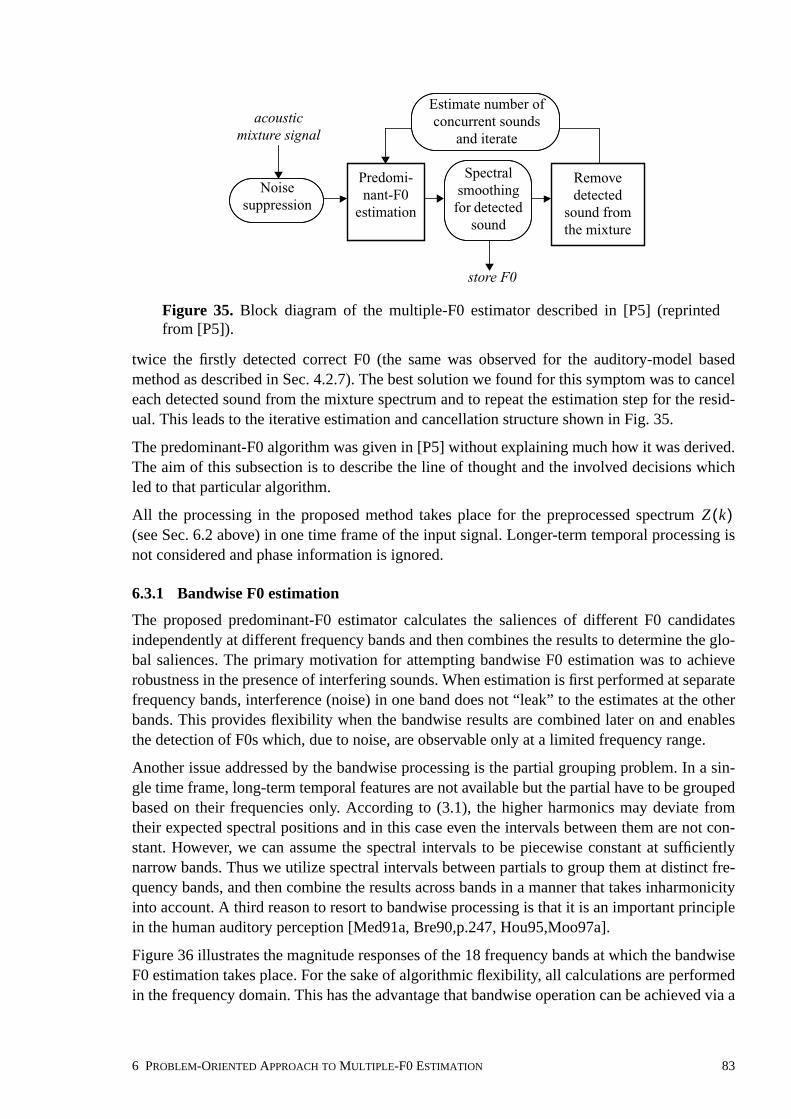
twice the firstly detected correct F0 (the same was observed for the auditory-model basedmethod as described in Sec. 4.2.7). The best solution we found for this symptom was to canceleach detected sound from the mixture spectrum and to repeat the estimation step for the resid-ual. This leads to the iterative estimation and cancellation structure shown in Fig. 35.
The predominant-F0 algorithm was given in [P5] without explaining much how it was derived.The aim of this subsection is to describe the line of thought and the involved decisions whichled to that particular algorithm.
All the processing in the proposed method takes place for the preprocessed spectrum(see Sec. 6.2 above) in one time frame of the input signal. Longer-term temporal processing isnot considered and phase information is ignored.
6.3.1 Bandwise F0 estimation
The proposed predominant-F0 estimator calculates the saliences of different F0 candidatesindependently at different frequency bands and then combines the results to determine the glo-bal saliences. The primary motivation for attempting bandwise F0 estimation was to achieverobustness in the presence of interfering sounds. When estimation is first performed at separatefrequency bands, interference (noise) in one band does not “leak” to the estimates at the otherbands. This provides flexibility when the bandwise results are combined later on and enablesthe detection of F0s which, due to noise, are observable only at a limited frequency range.
Another issue addressed by the bandwise processing is the partial grouping problem. In a sin-gle time frame, long-term temporal features are not available but the partial have to be groupedbased on their frequencies only. According to (3.1), the higher harmonics may deviate fromtheir expected spectral positions and in this case even the intervals between them are not con-stant. However, we can assume the spectral intervals to be piecewise constant at sufficientlynarrow bands. Thus we utilize spectral intervals between partials to group them at distinct fre-quency bands, and then combine the results across bands in a manner that takes inharmonicityinto account. A third reason to resort to bandwise processing is that it is an important principlein the human auditory perception [Med91a, Bre90,p.247, Hou95,Moo97a].
Figure 36 illustrates the magnitude responses of the 18 frequency bands at which the bandwiseF0 estimation takes place. For the sake of algorithmic flexibility, all calculations are performedin the frequency domain. This has the advantage that bandwise operation can be achieved via a
Remove
detected
sound from
the mixture
store F0
Predomi-
nant-F0
estimation
Estimate number of
concurrent sounds
and iterate
acousticmixture signal
Noise
suppression
Spectral
smoothing
for detected
sound
Figure 35. Block diagram of the multiple-F0 estimator described in [P5] (reprintedfrom [P5]).
Z k( )
6 PROBLEM-ORIENTED APPROACH TO MULTIPLE-F0 ESTIMATION 83
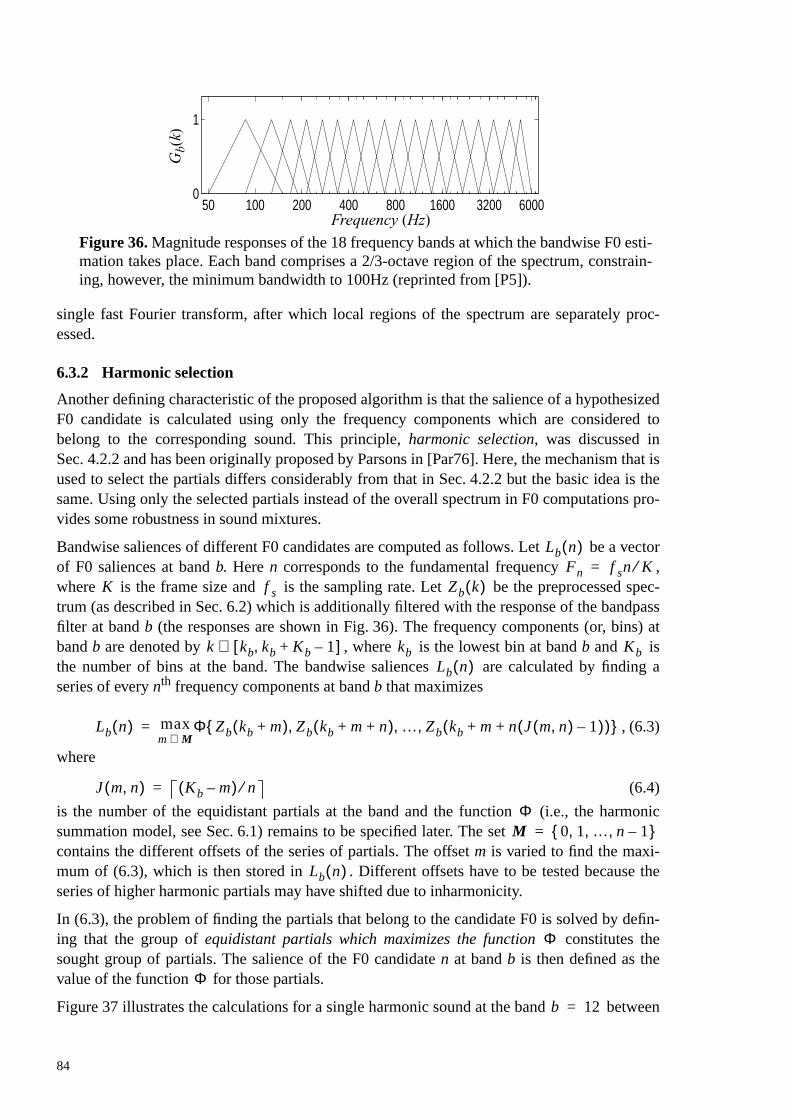
single fast Fourier transform, after which local regions of the spectrum are separately proc-essed.
6.3.2 Harmonic selection
Another defining characteristic of the proposed algorithm is that the salience of a hypothesizedF0 candidate is calculated using only the frequency components which are considered tobelong to the corresponding sound. This principle, harmonic selection, was discussed inSec. 4.2.2 and has been originally proposed by Parsons in [Par76]. Here, the mechanism that isused to select the partials differs considerably from that in Sec. 4.2.2 but the basic idea is thesame. Using only the selected partials instead of the overall spectrum in F0 computations pro-vides some robustness in sound mixtures.
Bandwise saliences of different F0 candidates are computed as follows. Let be a vectorof F0 saliences at band b. Here n corresponds to the fundamental frequency ,where is the frame size and is the sampling rate. Let be the preprocessed spec-trum (as described in Sec. 6.2) which is additionally filtered with the response of the bandpassfilter at band b (the responses are shown in Fig. 36). The frequency components (or, bins) atband b are denoted by , where is the lowest bin at band b and isthe number of bins at the band. The bandwise saliences are calculated by finding aseries of every nth frequency components at band b that maximizes
, (6.3)
where
(6.4)
is the number of the equidistant partials at the band and the function (i.e., the harmonicsummation model, see Sec. 6.1) remains to be specified later. The setcontains the different offsets of the series of partials. The offset m is varied to find the maxi-mum of (6.3), which is then stored in . Different offsets have to be tested because theseries of higher harmonic partials may have shifted due to inharmonicity.
In (6.3), the problem of finding the partials that belong to the candidate F0 is solved by defin-ing that the group of equidistant partials which maximizes the function constitutes thesought group of partials. The salience of the F0 candidate n at band b is then defined as thevalue of the function for those partials.
Figure 37 illustrates the calculations for a single harmonic sound at the band between
Frequency (Hz)
Gb(
k)
50 100 200 400 800 1600 3200 60000
1
Figure 36. Magnitude responses of the 18 frequency bands at which the bandwise F0 esti-mation takes place. Each band comprises a 2/3-octave region of the spectrum, constrain-ing, however, the minimum bandwidth to 100Hz (reprinted from [P5]).
Lb n( )Fn f sn K⁄=
K f s Zb k( )
k kb kb Kb 1–+,[ ]∈ kb KbLb n( )
Lb n( ) maxm M∈
Φ Zb kb m+( ) Zb kb m n+ +( ) … Zb kb m n J m n,( ) 1–( )+ +( ), , ,{ }=
J m n,( ) Kb m–( ) n⁄=
ΦM 0 1 … n 1–, , ,{ }=
Lb n( )
Φ
Φ
b 12=
84

1100Hz and 1700Hz. The arrows indicate the series of frequency components which maxi-mizes for the true F0 (corresponding to in this case).
The values of the offset m are further restricted to physically realistic inharmonicities, a subsetof M. The exact limit is not critical, therefore (3.1) with a constant inharmonicity factor
can be used to determine the maximum allowable offset from the ideal harmonicpositions. In the extreme case where there is only one harmonic partial at the band (i.e.
), inharmonicity is not allowed at all but the partial is selected from the ideal har-monic position in the spectrum. As a consequence, the “spectral-interval oriented” harmonicselection in (6.3) reduces to a special case where spectral-location information is used for har-monic selection.
6.3.3 Determining the harmonic summation model
The remaining problem is to determine the function in (6.3) which computes the salience ofa F0 candidate n based on the magnitudes of the selected harmonic components. We use
to denote the fundamental frequency corresponding to n. Also, we use todenote the set of the equidistant frequency bins at band b that maximizes (6.3) for candidate n.
The function was found via a two-stage process. As a starting point, we used a functionwhich estimates the perceived loudness of the set of the partials at band b. In the secondstep, the function was parametrized and machine-learning techiques were used to find suchparameters that, “most of the time”, the function gives the highest salience to the correct F0.
Given that the set for candidate n at band b contains at least one partial1, the loudness ofthe partials can be estimated as
, (6.5)
where is the power spectral density of the input signal at band b and isthe frequency of partial k (note that the above expression is used here as the backgroundmodel; the continuous power spectrum will be replaced by the noise-suppressed dis-crete spectrum in the following). The exponent 0.23 performs power spectrum compressionaccording to a recent model of loudness perception [Moo97b] and the overall sum approxi-mates the integral over the excitation pattern caused by partials on a critical-band scale.The coefficient
1. Inharmonicity is not allowed for the lowest partials as described in the previous subsection (Sec. 6.3.2).Consequently, there are frequency bands which do not contain any partials of a certain F0 candidate n.
1100 1200 1300 1400 1500 1600 1700
kb
kb+K
b−1
n=13m=11
Z 12(k
)Frequency (Hz)
Figure 37. Harmonic selection according to (6.3) (reprinted from [P5]).
L12 n( ) n 13=
β 0.01=
J m n,( ) 1=
Φ
Fn f sn K⁄= Obn( )
ΦOb
n( )
Obn( )
Lbˆ n( ) Ψxb
f k( )0.23 Fnddf-----e f k( )
k Ob
n( )∈∑=
Ψxbf( ) f k f sk K⁄=
Ψxbf k( )
Obn( )
6 PROBLEM-ORIENTED APPROACH TO MULTIPLE-F0 ESTIMATION 85

(6.6)
is the inter-partial interval around partial k on a critical-band scale. The mapping fromthe linear frequency scale to the critical-band scale is given by (4.6). Figure 38 illustrates thespectral area that is summed in (6.5), one critical band at a time. (Note that this model of loud-ness is simplified and does not limit the effect of the lowest partials to one critical band aroundthe partials.)
By derivating, it turns out that (6.6) is equal to , where is the ERB value ofthe auditory filter centered on and is a constant scalar which can be omitted. Note thatthis is equivalent to the concept of resolvability as defined in (4.57) on page 50. In order tosimplify (6.5), we replace by the bandwidths of the F0 estimator (see Fig. 36).The coefficient in (6.6) then, can be replaced by and (6.5) can be written in a simplifiedform as
. (6.7)
In a subsequent step, the above formula was parametrized and machine learning techniqueswere used to find the optimal values of the parameters. In the parametrized formula,
is used as the variable in place of . These two are closely related, as can beseen in (6.4). Also, is replaced by the discrete preprocessed spectrum . Thepreprocessing step involves compression and allows us to omit the exponent 0.23. The para-metrization of (6.7) is given as
, (6.8)
where the parameters and are to be learned1.
A well-posed machine-learning problem requires the definition of the task to do, the perform-ance measure to use, and the experience from which to learn [Mit97]. Here, the task assignedto the algorithm was to estimate the F0s of isolated musical sounds. The performance measureused was the percentage of cases where the maximum of at different bands corre-sponded to the true F0 of the sound in question. The learning algorithm had access to the cor-
1. It should be noted that the formula in (6.8) can no more be considered as estimating the loudness ofpartials . This is due to the described departures from the original model in (6.5). The loudnessmodel was used as a starting point but precise modeling of loudness as such is not of interest here.
Fnddf-----e f k( )
e f( )
1 5 10 15 20 25 30 35
1
23
45
6 78 9
50
Figure 38. The first 50 overtone partials of a harmonic sound (F0 140Hz) on a critical-band scale. The dotted vertical lines indicate the boundaries of adjacent critical bands.Expression (6.5) measures the area under the stepwise curve separately for each band b.
Critical-band scale e f( )
Ψx
f()0
.23
αFn u f k( )⁄ u f k( )f k α
u f k( ) f sKb K⁄n Kb⁄
Lb˜ n( ) n
Kb------ Ψxb
f k( )0.23
k Obn( )∈
∑=
1 J m n,( )⁄ n Kb⁄Ψxb
f k( )0.23 Zb n( )
Lb n( ) a0 a11
J m n,( )------------------+
Zb n( )k Ob
n( )∈∑=
a0 a1
Obn( )
Lb n( )
86

rect F0s of the sounds and attempted to improve the measure of success by changing the valuesof the coefficients and . As a results, the values and were learned.A second-order polynomial of was trained, too, but it did not perform significantlybetter than the first-order model which was therefore taken into use.
Thus, the function in (6.3) which computes the salience of a F0 candidate n at a fre-quency band b becomes
, (6.9)
where
(6.10)and is as defined in (6.4).
6.3.4 Cross-band integration and estimation of the inharmonicity factor
Figure 39 shows the calculated salience vectors at different bands for two isolated pianotones. The vectors are arranged in increasing band center frequency order. As expected, themaximum salience is usually assigned to the true F0, provided that there is a harmonic partialat that band. The inharmonicity phenomenon appears in the the two panels: the fundamentalfrequencies show a rising trend as a function of band center frequency.
The bandwise F0 saliences are combined to yield a global F0 estimate. A straightforward sum-mation across the salience vectors does not accumulate them appropriately since the F0 esti-mates at different bands may not match for inharmonic sounds, as can be seen in Fig. 39. Toovercome this, the inharmonicity factor is estimated and taken into account. Two differentinharmonicity models were implemented, the one given by (3.1) and another mentioned in[Fle98, p.363]. In simulations, the performance difference between the two was negligible. Themodel in (3.1) was adopted.
Global saliences L(n) are obtained by summing squared bandwise saliences that are
a0 a1 a0 0.25= a1 0.75=1 J m n,( )⁄
Lb n( )
Lb n( ) maxm M∈
c m n,( ) Zb kb m n j 1–( )+ +( )j 1=
J m n,( )
∑
=
c m n,( ) 0.25 0.75 J m n,( )⁄+=J m n,( )
0 50 100 150 200 250 300 350 400
87
170
270
428
680
1079
1713
2720
4317
0 100 200 300 400 500 600 700 800
87
170
270
428
680
1079
1713
2720
4317
Fundamental frequency (Hz)
Cen
ter
freq
uenc
y of
ban
ds(H
z)
Fundamental frequency (Hz)
Cen
ter
freq
uenc
y of
ban
ds(H
z)
Figure 39. Bandwise-calculated F0 saliences for two piano tones. The vectors aredisplaced vertically for clarity. The true F0s of the two sounds are 65Hz and 470Hz in theleft and right panels, respectively, and are indicated with dashed vertical lines (reprintedfrom [P5]).
Lb n( )
Lb n( )
Lb n( )
6 PROBLEM-ORIENTED APPROACH TO MULTIPLE-F0 ESTIMATION 87

selected from different bands according to a curve determined by (3.1). A search over possiblevalues of the inharmonicity factor is conducted for each n, and the highest and thecorresponding are stored in the output. Squaring the bandwise F0 saliences prior to sum-ming was found to provide robustness in very noisy cases where the pitch may be detectable ata limited frequency range only. Weighting of different bands according to their estimated sig-nal-to-noise ratios was not attempted.
The described method yields the inharmonicity factors (see (3.1)) of the detected sounds asa side-product. Figure 40 illustrates the measured inharmonicity factors for the differentnotes of an upright piano. The measured data agrees with that given by Fletcher and Rossingfor the piano in [Fle98, pp.363,390].
6.4 Coinciding frequency partials
The described predominant-F0 estimator operates reliably even in cases where several concur-rent harmonic sounds are present. However, the method is not able to estimate all the compo-nent F0s simultaneously but the iterative estimation and cancellation procedure shown inFig. 35 has to be applied.
The partials of a detected predominant-F0 cannot be completely removed from the mixturespectrum. This kind of “partial grouping” is not appropriate for coinciding partials1. The spec-tral components that are due to several coinciding partials need to be shared between the corre-sponding sounds. If the partials of a detected sound are completely removed, the coincidingpartials of other sounds are deleted in the subtraction procedure. After several iterations, asound remaining in the residual spectrum may become too corrupted to be correctly analyzedin the iterations that follow.
In addition to the above-described issue, coinciding partials of other sounds bring noise to theF0 salience calculations in (6.9). Although this problem is less severe, it sometimes causeserrors in the predominant-F0 estimation.
The aim of this section is to introduce two different techniques to deal with coinciding partials.The method proposed in [P3] is able to resolve coinciding partials to a certain degree and is
1. In practice, coinciding partials do not need to have exactly the same frequencies. The partials can beconsidered to coincide if their frequency difference is smaller than the width of the mainlobe of thespectrum of the time-domain analysis window.
β n( ) L n( )β n( )
β
Figure 40. Measured inharmonicity factors β for piano strings. The value β=0.0004given by Fletcher and Rossing [Fle98] for the middle register of the piano is indicatedwith a dashed horizontal line.
F4
β=0.0004
Fundamental frequency (Hz)
Inha
rmon
icit
y fa
ctor
33 65 131 262 523 1047 2093 4186 10
−5
10−4
10−3
10−2
C1 C2 C3 C4 C5 C6 C7 C8
β
88

introduced in Sec. 6.4.2. This mechanism is applied in the final system in Publication [P5]. Themethod introduced in Sec. 6.4.3 has been originally proposed in [P1] and is oriented towardsavoiding the use of coinciding partials when a sound is being observed.
6.4.1 Diagnosis of the problem
When two sinusoidal partials with amplitudes a1 and a2 and phase difference θ∆ coincide infrequency, the amplitude of the resulting sinusoid can be calculated as
. (6.11)
If the two amplitudes are roughly equivalent, the partials may either amplify or cancel eachother, depending on their phases. However, if one of the amplitudes is significantly larger thanthe other, as is usually the case, is close to the maximum of the two.
The condition that a harmonic partial h of a sound S coincides a harmonic j of another sound Rcan be written as , where FS and FR are the fundamental frequencies of the twosounds. Here ideal harmonicity is assumed, which is valid for many important classes of soundsources and for the lower-order harmonics ( ) of all the instruments considered in thiswork. When the common factors of integers h and j are reduced, we obtain
, (6.12)
where are integer numbers. This implies that partials of two sounds can coincideonly if the fundamental frequencies of the two sounds are in rational number relationships.Furthermore, when the fundamental frequencies of two sounds are in the above relationship,then every pth harmonic of the sound S coincides every qth harmonic of the sound R,where . This is evident since equals for each pair and ,when (6.12) holds. If , the sound R overlaps all the partials of sound S at their commonfrequency bands.
An important principle governing Western music is paying attention to the pitch relations,intervals, of simultaneously played notes. Simple harmonic relations satistying Eq. (6.12) arefavoured over dissonant ones. The smaller the values of p and q are, the closer is the harmonicrelation of the two sounds and the more perfectly they play together. For instance, fundamentalfrequencies in relationships 4 : 5: 6 constitute a basic major chord and fundamental frequen-cies in relationships : : constitute a basic minor chord. Because har-monic relations are so common in music, these “worst cases” must be handled well in general.Also, this partly explains why multiple-F0 estimation is particularly difficult in music.
Western music arranges notes to a quantized logarithmic scale1, where the fundamental fre-quency of a note n is Hz, and in the standard piano keyboard,for example. Although the scale is logarithmic, it can surprisingly well produce the differentharmonic F0 relationships that can be derived by substituting small integers to (6.12) [Kla98].Table 8 shows some basic musical intervals. As can be seen, the realizable F0 relationshipsdeviate a little from their harmonic ideals, but the amount of error is so small that it is notaurally disturbing to an average human listener. Moreover, for a feasible frequency analysisresolution, the coinciding of the partials appears as perfect2.
1. The scale is often called twelve tone equal-tempered scale.
as a1 a2eiθ∆+=
as
hFS jFR=
h 10<
FRpq---FS=
p q,( ) 1≥
pk qkk 1 2 …, ,= hFS jFR h pk= j qk=
p 1=
1 6⁄( ) 1 5⁄( ) 1 4⁄( )
Fn 440 2n 12⁄×= 48– n 39≤ ≤
6 PROBLEM-ORIENTED APPROACH TO MULTIPLE-F0 ESTIMATION 89

6.4.2 Resolving coinciding partials by the spectral smoothness principle
The amplitudes and phases of coinciding frequency partials can no more be deduced from theirsum. However, by making certain assumptions concerning the involved musical sounds, it ispossible to resolve the component partials to a certain degree. A method for this purpose hasbeen proposed in [P3] and is now introduced.
Consider the preprocessed spectrum of two concurrent harmonic sounds in Fig. 41. The F0s ofthe two sounds are in 1 : 3 relationships and, as a consequence, the partials of the higher-pitched sound coincide with every third harmonic of the lower-pitched sound. As predicted by(6.11), the coinciding partials randomly cancel or amplify each other at the low frequencies,whereas at the higher frequencies the summary amplitudes approach the maximum of the two,i.e., the spectral envelope of the higher sound.
In cases such as that in Fig. 41, the lower sound is usually detected first because it capturesmuch of the power of the higher-pitched sound, too. In general, sounds which are able to“steal” much of the energy of the other sounds are often detected first. Removing the partials ofthese sounds completely would effectively corrupt the other sounds.
2. The described principles generalize beyond Western music. Sethares has presented an extensive analy-sis of how music utilizes F0 relationships so as to cause partials of concurrent sounds coincide and tomake the sounds “blend” better [Set98]. Also, he draws an interesting connection between the appliedmusical instruments and the musical scales in different cultures.
Table 8: Some basic musical intervals.
Interval name Size (semitones)Ideal F0
relationship
Deviation from ideal
relationship
octave 12 2:1 0.0%
perfect fifth 7 3:2 –0.11%
perfect fourth 5 4:3 +0.11%
major third 4 5:4 +0.79%
minor third 3 6:5 –0.91%
major second 2 9:8 –0.23%
minor second 1 16:15 –0.68%
0 1000 2000 3000 4000 5000 60000
10
20
30
40
3
69 12
15 1821
2427
30
Frequency (Hz)
Mag
nitu
de o
fZ(k
)
Figure 41. Preprocessed spectrum Z(k) containing two sounds with F0s in the relation 1:3(reprinted from [P5]).
90
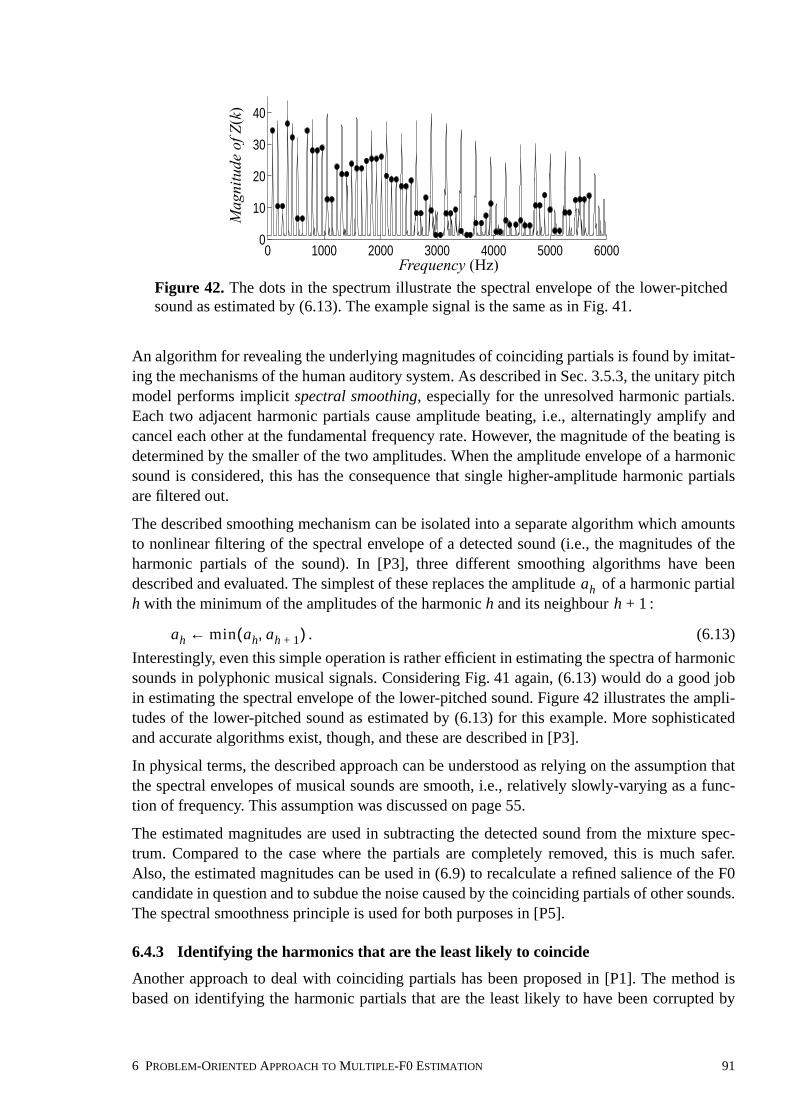
An algorithm for revealing the underlying magnitudes of coinciding partials is found by imitat-ing the mechanisms of the human auditory system. As described in Sec. 3.5.3, the unitary pitchmodel performs implicit spectral smoothing, especially for the unresolved harmonic partials.Each two adjacent harmonic partials cause amplitude beating, i.e., alternatingly amplify andcancel each other at the fundamental frequency rate. However, the magnitude of the beating isdetermined by the smaller of the two amplitudes. When the amplitude envelope of a harmonicsound is considered, this has the consequence that single higher-amplitude harmonic partialsare filtered out.
The described smoothing mechanism can be isolated into a separate algorithm which amountsto nonlinear filtering of the spectral envelope of a detected sound (i.e., the magnitudes of theharmonic partials of the sound). In [P3], three different smoothing algorithms have beendescribed and evaluated. The simplest of these replaces the amplitude of a harmonic partialh with the minimum of the amplitudes of the harmonic h and its neighbour :
. (6.13)
Interestingly, even this simple operation is rather efficient in estimating the spectra of harmonicsounds in polyphonic musical signals. Considering Fig. 41 again, (6.13) would do a good jobin estimating the spectral envelope of the lower-pitched sound. Figure 42 illustrates the ampli-tudes of the lower-pitched sound as estimated by (6.13) for this example. More sophisticatedand accurate algorithms exist, though, and these are described in [P3].
In physical terms, the described approach can be understood as relying on the assumption thatthe spectral envelopes of musical sounds are smooth, i.e., relatively slowly-varying as a func-tion of frequency. This assumption was discussed on page 55.
The estimated magnitudes are used in subtracting the detected sound from the mixture spec-trum. Compared to the case where the partials are completely removed, this is much safer.Also, the estimated magnitudes can be used in (6.9) to recalculate a refined salience of the F0candidate in question and to subdue the noise caused by the coinciding partials of other sounds.The spectral smoothness principle is used for both purposes in [P5].
6.4.3 Identifying the harmonics that are the least likely to coincide
Another approach to deal with coinciding partials has been proposed in [P1]. The method isbased on identifying the harmonic partials that are the least likely to have been corrupted by
ahh 1+
ah min ah ah 1+,( )←
0 1000 2000 3000 4000 5000 60000
10
20
30
40
Mag
nitu
de o
fZ(k
)
Frequency (Hz)
Figure 42. The dots in the spectrum illustrate the spectral envelope of the lower-pitchedsound as estimated by (6.13). The example signal is the same as in Fig. 41.
6 PROBLEM-ORIENTED APPROACH TO MULTIPLE-F0 ESTIMATION 91

the coinciding partials of other sounds. Those partials are then given more weight when mak-ing observations concerning a hypothesized harmonic sound in a mixture signal.
The starting point of the method in [P1] is the assumption that if a harmonic sound S with fun-damental frequency occurs in music, it is quite probable that other harmonic sounds Riwith fundamental frequencies (here integers ) occur simultane-ously. This is due to the principles of Western music as discussed in Sec. 6.4.1. Moreover, it isreasonable to assume that all values of p and q binding the fundamental frequencies areequally probable, except that small values are in general more probable than large values. As aconsequence, the partials of an interfering sound Ri are equally probable to overlap any subsetof every pth partial of S. The set of every pth partial of S is here denoted by
. (6.14)
Let us denote by the probability that an interfering sound Ri overlaps some subset ofthe sound S. The probability is assumed to be the same for all the sets as mentionedabove. However, the likelihood that an individual harmonic partial does not coincide with thepartials of the other sounds is not equal to all different harmonics h. Instead, the likelihood isproportional to the probability that none of the sets that the partial h belongs to is over-lapped. This can be calculated as , where is the number of subsets thatthe harmonic h belongs to. It is easy to prove that is the number of integers that divide h,
. An integer a is defined to divide another integer b, if and only if for someinteger d. Here, perfect harmonicity is assumed.
The method in [P1] utilizes the above analysis in order to make reliable observations of a har-monic sound in polyphonic musical signals. The most fundamental observation, of course, iswhether a hypothesized sound exists in the mixture signal or not. This is reduced to the ques-tion whether the individual harmonics of a sound appear in the spectrum or not. However, thereare two types of outlier partials, i.e., harmonics that are not valid to represent a hypothesizedsound. Some harmonics may be due to the coinciding partials of other sounds only, whereassome harmonics may be missing from the target sound even when it is present. In [P1], aweighted order-statistical filter [Kuo94, Ast97] is proposed which is able to filter out the out-lier values. Moreover, the sample selection probabilities of the filter are set according to therelative trustworthiness of different harmonics. The hth sample selection probability is theprobability that the sample h in a set is selected to the output of the filter [Kuo94].
A complete description of the method can be found in [P1]. The method has been extensivelyused in a transcription system for piano music as described in [Kla98]. The method as such isnot applied in the multiple-F0 estimation method in [P5]. However, a spectral smoothing algo-rithm which utilizes the statistical dependencies of the subsets achieves a slight improve-ment in [P5].
6.5 Criticism
The multiple-F0 estimation method described in this chapter has a certain major weakness.That is, the iterative cancellation of the detected sounds is performed by separating the spectraof the sounds in the frequency domain. Estimation and separation of the individual higher-order harmonic partials cannot be done reliably. The smoothing mechanism partly saves theday because it prevents from completely removing the higher-order partials and thus fromdestroying the corresponding frequency range of the mixture spectrum.
FSFRi
p q⁄( )FS= p q,( ) 1≥
FRi
E p pk{ } k 1 2 …, ,=,=
π0 E pπ0 E p
E p1 π0–( )D h( ) D h( ) E p
D h( )D 1( ) 1= b da=
E p
92
The successfulness of the frequency-domain separation depends critically on the resolution ofthe spectrum. As a consequence, the described method requires a relatively long analysis frameto perform well. The method proposed in Chapter 4 is advantageous in this respect because ituses a different mechanism to estimate and cancel the higher-order (unresolved) partials. As aresult, the method in Chapter 4 achieves a better accuracy, particularly in shorter time frames,as can be seen in Table 6 on page 65.
The method presented here has some advantages compared to that in Chapter 4, as well. Thesewere mentioned in the beginning of this chapter.
6 PROBLEM-ORIENTED APPROACH TO MULTIPLE-F0 ESTIMATION 93

94
7 Conclusions and future work
7.1 Conclusions
7.1.1 Multiple-F0 estimation
Main part of this thesis deals with multiple-F0 estimation which was considered to be the coreof the music transcription problem. Two different methods were proposed for this purpose. Thefirst was derived from the unitary pitch model in Chapter 4 and the other, as originally pub-lished in [P5], is oriented towards more pragmatic problem-solving. The obtained results indi-cate that multiple-F0 estimation can be performed reasonably accurately at the level of a singletime frame. For a variety of musical sounds, a priori knowledge of the sound sources is notnecessary, although this might further improve the performance.
The method described in [P5] represents a “complete” multiple-F0 estimation system in thesense that it includes mechanisms for suppressing additive noise and for estimating the numberof concurrent sounds in an input signal. Also, it provides an explicit reference implementationof many basic mechanisms that are needed in multiple-F0 estimation. However, the methoddescribed in Chapter 4 is more accurate and, in particular, operates more reliably in short anal-ysis frames. A comparative evaluation of the two methods was presented in Table 6 on page65. The performance advantage of the method described in Chapter 4 is due to the principlethat higher-order (unresolved) harmonic partials are processed collectively; estimation andseparation of individual higher-order partials is not attempted. The author of this work wasquite surprised at the efficiency of the combined use of spectral-location and spectral-intervalinformation, basically directly according to the model for half-wave rectification in (4.27).
Both of the proposed multiple-F0 estimation methods are based on an iterative estimation-and-cancellation approach. The method described in [P5] separates the spectra of detected soundsfrom the mixture, whereas the method described in Chapter 4 does not separate but, rather,cancels the effect of detected sounds from the mixture signal. The very reason to resort to theiterative approach was that we could not find any other technique that would have led to a com-parable degree of accuracy. A particularly attractive property of the iterative approach is that atleast a couple of the most prominent F0s can be detected even in rich polyphonies. The proba-bility of error increases rapidly in the course of iteration but, as described in [P5], this appearsto be at least partly due to the inherent characteristics of the problem itself: some sounds in amixture signal are more difficult to detect and remain in the residual till the last iterations. Thesounds which are aurally the most prominent are usually detected first.
It seems unlikely that the frame-level multiple-F0 estimation accuracy could get substantiallybetter using bottom-up signal analysis techniques. The two methods converge close to thesame error rate (although the auditory-model based method is superior in short analysisframes) and the performance of both methods is comparable to that of human listeners, asdescribed in [P5]. However, substantial performance improvements can still be expected byutilizing longer-term acoustic features and by constructing internal musicological models orsound sources models. These will be discussed in Sec. 7.2 below.
7.1.2 Musical meter estimation
The proposed musical meter estimator is fairly successful in estimating the meter of different
7 CONCLUSIONS AND FUTURE WORK 95

types of music signals. This conclusion was drawn by comparing the obtained results withthose of the two reference systems in Publication [P6] and, informally, by auralizing meterestimatimation results as a generated drum track along with the original piece.
As mentioned in Sec. 1.3, pitch information is not utilized in meter estimation. This basic deci-sion contradicts with what we know about the human cognition of music but, nevertheless, wasmade for two main reasons. First, the proposed meter analysis is computationally very efficientcompared to the multiple-F0 analysis. Secondly, the meter estimator benefits of a relativelygood time-resolution which cannot be adequately provided by the multiple-F0 estimators. Thedisadvantage of ignoring the pitch information is that meter analysis at the measure-pulse levelis not very reliable. Since the measure-pulse correlates with harmonic changes, pitch informa-tion would most probably improve the accuracy. Despite this criticism, the simulation resultsindicate that the meter of a large part of musical material can be analyzed without resorting tomultiple-F0 analysis. The most important elements of a successful meter estimator turned outto be measuring the degree of musical accentuation as a function of time and modeling primi-tive musical knowledge which governs musically meaningful meter abstractions.
7.2 Future work
7.2.1 Musicological models
The scope of this thesis was restricted to bottom-up signal analysis methods. As mentioned inSec. 1.2.2, however, the use of musicological information is almost equally important in theautomatic transcription of real-world musical material. Although the accuracy of the proposedmultiple-F0 methods is comparable to that of trained humans in musical-chord identificationtasks, the accuracy of the methods is still inferior in the transcription of continuous musicalpieces. This is largely due to the fact that the proposed methods do not include any internal“language model” for music but, instead, consider each individual analysis frame separately,apart from its context. Temporal continuity of musical sounds or melodic phrases is not takeninto account at all. In brief, the program performs multiple-F0 estimation but it does not under-stand anything about music. Demonstrations of the transcription of continuous musical piecesusing the described musically-agnostic system are available at [Kla03b].
There are straightforward and efficient ways of representing musicological knowledge. As anexample, consider the following experiment. We represented combinations of co-occurringnotes as 12-bit numbers that we call chord unigrams. There are 4096 such unigrams. Each bitsignifies the presence/absence of one of the 12 pitch classes1. A total of 359 MIDI songs werecollected and cut into segments where note onsets and offsets do not occur. The harmonic con-tent of each segment was then represented with the corresponding unigram. The probability ofoccurrence for each unigram was computed within the pieces and averaged over all pieces. Theresults were interesting: among the 30 most probable unigrams were the 12 single notes (pitchclasses), seven different major triad chords, five minor triads, and three minor-seventh chords.
The described kind of “brute force” statistical approach has several advantages. First, the esti-mated prior probabilities of different F0 combinations can be used to rate the likelihoods ofseveral competing F0 hypotheses in a transcription system. Secondly, the described estimation
1. The pitch class “c”, for example, represents all c notes in different octaves since these play the sameharmonic role. The principle that the notes c3 (130Hz), c4 (260Hz), c5 (520Hz) etc. are consideredequivalent is called octave equivalence. The twelve pitch classes are: c, c#, d, d#, e, f, f#, g, g#, a, a#, h.
96

procedure involves no heuristic parameters or rules. Thirdly, no musical expertise wasemployed, yet the system knows about major and minor triad chords, the building blocks ofWestern harmony. New music types can be addressed simply by re-estimating the unigramprobabilities using different training material.
The described experiment with chord unigrams is merely an example of the probabilisticapproach to musicological modeling. Similar formulations can be proposed for the temporalcontinuity of melodies and for harmonic progression, for example. Readily-collected statisticshave been published e.g. in [Kru90, pp. 67, 181, 195]. More complex rules governing Westernmusic can be found in music-theory workbooks. Temperley has proposed a very comprehen-sive rule-based system which models the cognition of basic musical structures [Tem01]. Heused the system for the automatic musicological analysis of MIDI files. From the point of viewof music transcription, a remaining challenge is to transform these rule-based models intoprobabilistic models which are able to evaluate the likelihoods of several candidate analysesalready during the transcription process.
7.2.2 Utilizing longer-term temporal features in multiple-F0 estimation
In Sec. 5.2.1, several perceptual cues were listed which promote the grouping of time-fre-quency components to a same sound source in human listeners. The cues, when present, facili-tate the auditory organization (analysis) of sound mixtures. The proposed multiple-F0estimators utilize two cues extensively: harmonic frequency relationships of partials and spec-tral smoothness of their amplitude values. In contrast to this, a certain important feature wasnot utilized at all: synchronous changes of time-frequency components. For example, the com-ponents belonging to a same sound typically set on simultaneously, they may exhibit synchro-nous frequency-modulation (vibrato) or amplitude-modulation, or the components may have a“common fate”, such as synchronously ascending frequencies. All these cues are commonlypresent in real-world music signals.
There is a straightforward way of utilizing the longer-term temporal features in multiple-F0estimation. The proposed multiple-F0 estimation methods perform the analysis in a single timeframe. Moreover, the analysis frames can be relatively short (down to 46ms) in the case of theauditory-model based method. Taking hanning-windowing into account, it is meaningful tocompute the F0-salience vectors every 23 milliseconds. Consider calculating the differ-ence between two temporally successive F0-salience vectors, . In a quitetypical musical situation, several long-duration notes are playing in the background and, on topof this static harmonic background, a sequence of shorter notes (a melody) is played. When anew sound sets on, it appears as a peak in the differential F0-salience, whereas the long-dura-tion notes do not pop up because they are present in both the past and the future frames. Inother words, the differential includes only the freshly onsetting sound and, from the point ofview of the differential F0-salience, the polyphony is virtually one in this case.
The above-described principle can be used to model all the “synchronous changes” cues. Aclear peak in the differential F0-salience vector occurs exactly when all the partials of a certainF0 change synchronously. For example, when several sounds are playing and only one of thesounds exhibits vibrato, the sound with vibrato comes up in the differential F0-salience. This isbecause the peaks corresponding to the vibrato-sound in successive F0-salience vectors are indifferent positions . In a practical implementation, instead of merely picking maxima in theF0-salience vectors themselves, it might be reasonable to inspect the differential of F0-sali-
λ τ( )λ t 1+( ) τ( ) λ t( ) τ( )–
τ
7 CONCLUSIONS AND FUTURE WORK 97

ence, too, or, to pick peaks in the weighted sum of the two. From the point of view of psychoa-coustics, we know that the auditory-nerve response is very strong at the onset of a sound butthen steadily falls to a lower “adaptation” level when the sound continues playing [Med86].The use of differential F0-salience would not depart much from this basic principle and is ableto model the perceptual effect of the “synchronous changes” cues in auditory organization.
7.3 When will music transcription be a “solved problem”?
An important fact about music transcription is that it is difficult. The problem is at best compa-rable to automatic speech recognition which has been studied for fifty years and is only nowbecoming practically applicable. In music transcription, the development will probably befaster as the computational power is already available and we can borrow theoretical methodsand approaches from speech recognition. However, the problem is really not in finding fastcomputers but in discovering the mechanisms and principles that humans use when listening tomusic. Modelling perception is difficult because the world in which we live is complex,because the things that humans create are complex (music being just one example), andbecause the human brain is complex.
Anyone who claims to have a quick solution to the polyphonic transcription problem, or a sin-gle mechanism that solves the problem once and for all – is mistaken. The human brain com-bines a large number of processing principles and heuristics. We will be searching for them foryears, perhaps even decades, before arriving at, say, 95% of a skilled musician’s accuracy andflexibility.
There is a certain factor which may crucially change the above prediction regarding the timeneeded to release an accurate general-purpose1 music transcriber. This has to do with the gen-erative nature of music versus speech. The development of speech recognition systems is con-stantly confronted with the problem that the amount of targeted and carefully annotatedtraining data is limited. Synthetic speech is not valid for training a speech recognizer. In musictranscription, the very problem stems from combinatorics: the sounds of different instrumentsoccur in varying combinations and make up musical pieces. The dynamic variability and com-plexity of a single sound event is not as high as that of speech sounds2. For these reasons, weargue that synthetic music is valid for training a music transcriber. In principle, astronomicalamounts of training data can be generated since acoustic measurements for isolated musicalsounds are available, combinations of these can be generated by mixing, and effects can beadded. An exact reference annotation is immediately available.
The availability of training data helps us to automatize away the most frustrating part of algo-rithm development: parameter optimization. However, it does not free us from designing themethods themselves. It is quite unlikely that the transcription problem could be solved simplyby training a huge neural network, for example. The “space” of possible algorithms and mod-els may be even larger than we can think of. The interesting part is to explore this space in ameaningful and efficient way until we have found the necessary ingredients of a successfultranscription system. People from different disciplines are needed in this pursuit, including sig-nal processing, acoustics, computer science, music, linguistics, and experimental psychology.
1. The concept music is not well-defined: in principle anything can be called music. The scope of a “gen-eral-purpose” transcriber is here limited to signal types that are commonly regarded as music.
2. Even for singing, transcribing the melody is significantly easier than recognizing the lyrics.
98

Bibliography
[Abd03] S. A. Abdallah and M. D Plumbley, “Probability as metadata: Event detection inmusic using ICA as a conditional density model,” In Proc. 4th International Symposium onIndependent Component Analysis and Blind Signal Separation, Nara, Japan, April 2003.
[Abd_] S. A. Abdallah and M. D. Plumbley, “Sparse coding of music signals,” Submitted toNeural Computation.
[AKo01] AKoff Sound Labs, AKoff Music Composer (transcription software), 2001.URL: http://www.akoff.com/
[Ale01] J. S. Alexander, K. A. Daniel, and T. G. Katsianos, “Apparatus for detecting the funda-mental frequencies present in polyphonic music,” United States Patent Application Publica-tion, Pub. No. US 2001/0045153 A1, Nov. 29, 2001.
[All90] P. E. Allen and R. B. Dannenberg, “Tracking Musical Beats in Real Time,” In Proc.International Computer Music Conference, San Francisco, 1990.
[Ara03] Arakisoftware, AmazingMIDI (transcription software), 2003.URL: http://www.pluto.dti.ne.jp/~araki/amazingmidi/
[ANS73] American National Standards Institute, ANSI. Psychoacoustical terminology. Amer-ican National Standards Institute, New York, 1973.
[Ast97] J. T. Astola and P. Kuosmanen, Fundamentals of Nonlinear Digital Filtering. CRCPress, 1997.
[Bar01] J. Barker, M. Cooke, and P. Green, “Robust ASR Based On Clean Speech Models: AnEvaluation of Missing Data Techniques For Connected Digit Recognition in Noise,” inProc. Eurospeech, Aalborg, Denmark, 2001.
[Bel99] S. D. Bella and I. Peretz, “Music agnosias: Selective impairments of music recognitionafter brain damage,” Journal of New Music Research, 28(3), 209–216, 1999.
[Bel03] J. P. Bello, “Towards the Automated Analysis of Simple Polyphonic Music: A Knowl-edge-Based Approach,” Ph.D. thesis, Univ. of London, 2003.
[Bil93] J. Bilmes, “Timing is of the Essence: Perceptual and Computational Techniques forRepresenting, Learning, and Reproducing Expressive Timing in Percussive Rhythm,” M.Sc.thesis, Massachusetts Institute of Technology, 1993.
[Bra99] M. Braun, “Auditory midbrain laminar structure appears adapted to f0 extraction: fur-ther evidence and implications of the double critical bandwidth,” Hearing Res., 129, 71–82,1999.
[Bra00] M. Braun, “Inferior colliculus as candidate for pitch extraction: multiple support fromstatistics of bilateral spontaneous otoacoustic emissions,” Hearing Res. 145, 130–140,2000.
[Bre90] A. S. Bregman, Auditory Scene Analysis. The MIT Press, Cambridge, Massachusetts,1990.
[Bro92a] G. J. Brown. “Computational auditory scene analysis: A representational approach,”Ph.D. thesis, Dept. of Comp. Sci., Univ. of Sheffield, 1992.
[Bro94] G. J. Brown and M. Cooke, “Perceptual grouping of musical sounds: A computationalmodel,” J. of New Music Research 23, 107–132, 1994.
[Bro91] J. C. Brown and B. Zhang, “Musical frequency tracking using the methods of conven-
BIBLIOGRAPHY 99

tional and “narrowed” autocorrelation,” J. Acoust. Soc. Am., 89 (5), 2346–2354, 1991.
[Bro92b] J. C. Brown, “Musical fundamental frequency tracking using a pattern recognitionmethod,” J. Acoust. Soc. Am., 92 (3), 1394–1402, 1992.
[Bro93a] J. C. Brown, “Determination of the meter of musical scores by autocorrelation,” J.Acoust. Soc. Am., 94 (4), 1953-1957, 1993.
[Bro01] J. C. Brown, “Feature dependence in the automatic identification of musical wood-wind instruments,” J. Acoust. Soc. Am., 109 (3), 1064-1072, 2001.
[Bro93b] L. Brown (Ed.), The New Shorter Oxford English Dictionary. Oxford UniversityPress, New York, 1993.
[Bui04] BuildOrBuy Group Network, List of Wav to Midi conversion and audio transcriptionsoftware, 2004. URL: http://www.buildorbuy.org/wavtomidi.html
[Car92] N. Carver and V. Lesser, “The evolution of blackboard control architectures,” Massa-chusetts Amherst University Technical Report 92-71, Oct. 1992.
[Cem01] A. T. Cemgil, B. Kappen, P. Desain, and H. Honing, “On tempo tracking: Tempo-gram representation and Kalman filtering,” Journal of New Music Res., 28(4), 259–273,2001.
[Cem03] A. T. Cemgil and B. Kappen, “Monte Carlo Methods for Tempo Tracking andRhythm Quantization,” Journal of Artificial Intelligence Research 18, 45-81, 2003.
[Cha82] C. Chafe, B. Mont-Reynaud, and L. Rush, “Toward an Intelligent Editor of DigitalAudio: Recognition of Musical Constructs”. Computer Music Journal, 6 (1), Spring 1982.
[Cha86a] C. Chafe and D. Jaffe, “Source separation and note identification in polyphonicmusic,” in Proc. IEEE International Conf. on Acoust., Speech, and Signal Processing,Tokyo, 1986.
[Cha86b] C. Chafe and D. Jaffe, “Techniques for Note Identification in Polyphonic Music,” inProc. IEEE International Conference on Acoustics Speech and Signal Processing, Tokyo,1986.
[Cla02] L. P. Clarisse, J. P. Martens, M. Lesaffre, B. De Baets, H. De Mayer, and M. Leman,“An Auditory Model Based Transcriber of Singing Sequences,” In Proc. International Con-ference on Music Information Retrieval, Paris, France, Oct. 2002.
[Cla99] E. F. Clarke, “Rhythm and Timing in Music,” In The Psychology of Music, D. Deutsch,(Ed.), Academic Press, 1999.
[Cla04] Classical Archives LLC, Classical Archives (an archive of classical music), 2004.URL: http://www.classicalarchives.com/
[Coo91] M. Cooke. “Modelling Auditory Processing and Organisation,” Ph.D thesis, Dept. ofComp. Sci., Univ. of Sheffield, 1991.
[Coo94] M. Cooke and G. J. Brown, “Separating Simultaneous Sound Sources: Issues, Chal-lenges and Models,” in Fundamentals of speech synthesis and speech recognition, E. Keller,(Ed.), J. Wiley, pp. 295-312, 1994.
[Coo01a] M. Cooke and D. P. W. Ellis “The auditory organization of speech and other sourcesin listeners and computational models,” Speech Communication, 35(3–4), 141–177, 2001.
[Coo01b] M. Cooke, P. Green, L. Josifovski, and A. Vizinho, “Robust automatic speech recog-nition with missing and unreliable acoustic data,” Speech Communication, 34 (3), 267–285,2001.
100

[Cor90] T. H. Cormen, C. E. Leiserson, and R. L. Rivest, Introduction to Algorithms. MITPress, Cambridge, Massachusetts, 1990.
[Dav02] M. Davy and S. Godsill, “Detection of Abrupt Spectral Changes using Support VectorMachines. An application to audio signal segmentation,” In Proc. IEEE International Con-ference on Acoustics, Speech, and Signal Processing, Orlando, Florida, May 2002.
[Dav03] M. Davy and S. J. Godsill, “Bayesian harmonic models for musical signal analysis, ”In Bayesian Statistics VII, J.M. Bernardo, J.O. Berger, A.P. Dawid, and A.F.M. Smith(Eds.), Oxford University Press, 2003.
[Dav87] W. B. Davenport and W. L. Root, An Introduction to the Theory of Random Signalsand Noise, IEEE Press, 1987.
[deC93] A. de Cheveigné, “Separation of concurrent harmonic sounds: fundamental frequencyestimation and a time-domain cancellation model of auditory processing,” J. Acoust. Soc.Am., 93 (6), 3271–3290, 1993.
[deC99] A. de Cheveigné and H. Kawahara, “Multiple period estimation and pitch perceptionmodel,” Speech Communication 27, 175–185, 1999.
[deC01] A. de Cheveigné and H. Kawahara, “Comparative evaluation of F0 estimation algo-rithms,” in Proc. Eurospeech, Copenhagen, Denmark, 2001.
[deC02] A. de Cheveigné and H. Kawahara, “YIN, a fundamental frequency estimator forspeech and music,” J. Acoust. Soc. Am., 111 (4), April 2002.
[Dep93] Ph. Depalle, G. García, and X. Rodet, “Tracking of partials for additive sound synthe-sis using hidden Markov models,” In Proc. IEEE International Conference on Acoustics,Speech and Signal Processing, Minneapolis, Minnesota, 1993.
[Dep97] Ph. Depalle and T. Hélie, “Extraction of spectral peak parameters using a short-timeFourier transform modeling and no sidelobe windows,” In Proc. IEEE Workshop on Appli-cations of Signal Processing to Audio and Acoustics, New Paltz, New York, 1997.
[Des99] P. Desain and H. Honing, “Computational models of beat induction: the rule-basedapproach,” Journal of New Music Research, 28 (1), 29-42, 1999.
[Deu99] D. Deutsch (Ed.), The Psychology of Music. Academic Press, San Diego, 1999.
[Dix01] S. Dixon, “Automatic Extraction of Tempo and Beat from Expressive Performances,”J. New Music Research 30 (1), 39-58, 2001.
[Dov91] B. Doval and X. Rodet, “Estimation of fundamental frequency of musical sound sig-nals,” in Proc. IEEE International Conf. on Acoust., Speech, and Signal Processing, 1991.
[Dov93] B. Doval and X. Rodet. “Fundamental frequency estimation and tracking using maxi-mum likelihood harmonic matching and HMM’s,” In Proc. IEEE International Conferenceon Acoustics, Speech and Signal Processing, 1993.
[Dun61] H. K. Dunn, “Methods of Measuring Vowel Formant Bandwidths,” J. Acoust. Soc.Am., 33 (12), 1737–1746, 1961.
[Dux03] C. Duxbury, J. P. Bello, M. Davies, and M. Sandler, “Complex domain onset detectionfor musical signals,” In Proc. 6th Int. Conference on Digital Audio Effects, London, UK,Sep. 2003.
[Ell95] D. P. W. Ellis and D. F Rosenthal, “Mid-level representations for Computational Audi-tory Scene Analysis,” In Proc. Workshop on Computational Auditory Scene Analysis, Intl.Joint Conf. on Artif. Intell., Montreal, Aug. 1995.
BIBLIOGRAPHY 101
[Ell96] D. P. W. Ellis, “Prediction-driven computational auditory scene analysis,” Ph.D. thesis,MIT Media Laboratory, Cambridge, Massachusetts, 1996.
[Ero00] A. Eronen and A. P. Klapuri, “Musical instrument recognition using cepstral coeffi-cients and temporal features,” In Proc. IEEE International Conference on Acoustics, Speechand Signal Processing, Istanbul, Turkey, June 2000.
[Ero01] A. Eronen, “Comparison of features for musical instrument recognition,” In Proc.IEEE Workshop on Applications of Signal Processing to Audio and Acoustics, New Paltz,New York, Oct. 2001.
[Fiz02] D. FitzGerald, E. Coyle, and B. Lawlor, “Sub-band Independent Subspace Analysis forDrum Transcription”, in Proc. 5th Int. Conference on Digital Audio Effects (DAFX-02),Hamburg, Germany, 2002.
[Fle40] H. Fletcher, “Auditory patterns,” Reviews of Modern Physics, 12, 47–65, 1940.
[Fle98] N. F. Fletcher and T. D. Rossing, The physics of musical instruments. 2nd ed.Springer–Verlag New York, 1998.
[Gla90] B. R. Glasberg and B. C. J. Moore, “Derivation of auditory filter shapes from notched-noise data,” Hearing Research 47, 103–138, 1990.
[God98] D. Godsmark, “A computational model of the perceptual organization of polyphonicmusic,” Ph.D. thesis, Dep. of Comp. Sc., Univ. of Sheffield, 1998.
[God99] D. Godsmark and G. J. Brown, “A blackboard architecture for computational auditoryscene analysis,” Speech Communication 27, 351–366, 1999.
[Gom03] E. Gómez, A. Klapuri, and B. Meudic, “Melody Description and Extraction in theContext of Music Content Processing,” Journal of New Music Research, 32 (1), 2003.
[Gol73] J. L. Goldstein, “An optimum processor theory for the central formation of the pitch ofcomplex tones,” J. Acoust. Soc. Am., 54 (6), 1973.
[Goo97] M. M. Goodwin, “Adaptive Signal Models: Theory, Algorithms, and Audio Applica-tions,” Ph.D. thesis, Univ. of California, Berkeley, 1997.
[Got95] M. Goto and Y. Muraoka, “Music understanding at the beat level — real-time beattracking for audio signals,” In Working Notes of the IJCAI-95 Workshop on ComputationalAuditory Scene Analysis, 1995, pp. 68-75.
[Got96] M. Goto and Y. Muraoka, “Beat Tracking based on Multiple-agent Architecture — AReal-time Beat Tracking System for Audio Signals,” In Proc. Second International Confer-ence on Multiagent Systems, 1996, pp.103–110.
[Got97] M. Goto and Y. Muraoka, “Real-time Rhythm Tracking for Drumless Audio Signals— Chord Change Detection for Musical Decisions,” In Proc. IJCAI-97 Workshop on Com-putational Auditory Scene Analysis, 1997, pp. 135-144.
[Got00] M. Goto, “A robust predominant-F0 estimation method for real-time detection of mel-ody and bass lines in CD recordings,” in Proc. IEEE International Conf. on Acoust., Speech,and Signal Processing, Istanbul, Turkey, June 2000.
[Got01] M. Goto, “A predominant-F0 estimation method for real-world musical audio signals:MAP estimation for incorporating prior knowledge about F0s and tone models,” in Proc.Workshop on Consistent and reliable acoustic cues for sound analysis, Aalborg, Denmark,Sep. 2001.
[Gou01] F. Gouyon and P. Herrera, “Exploration of techniques for automatic labeling of audiodrum tracks’ instruments”, in Proc. MOSART: Workshop on Current Directions in Compu-
102
ter Music, Barcelona, Spain, 2001.
[Gou02] F. Gouyon, P. Herrera, and P. Cano, “Pulse-dependent analyses of percussive music,”In Proc. AES 22nd International Conference on Virtual, Synthetic and Entertainment Audio,Espoo, Finland, June 2002.
[Gus02] S. Gustafsson, R. Martin, P. Jax, and P. Vary, “A Psychoacoustic Approach to Com-bined Acoustic Echo Cancellation and Noise Reduction,” IEEE Trans. Speech and AudioProc. 10(5), July 2002.
[Hai01] S. W. Hainsworth, “Analysis of Musical Audio for Polyphonic Transcription,” 1st yearreport, Dept. of Eng., Univ. of Cambridge, 2001.
[Hai02] S. W. Hainsworth and M. D. Macleod, “A Physiologically Motivated Approach toMusic Transcription,” Poster presented at the Digital Music Research Network Launch Day,Dec. 17th, 2002.
[Hai_] S. W. Hainsworth, “Techniques for the Automated Analysis of Musical Audio,” Ph.Dthesis, Cambridge Univ., to appear.
[Han95] S. Handel, “Timbre perception and auditory object identification,” In Hearing —handbook of perception and cognition, B. C. J. Moore (Ed.), Academic Press, San Diego,California, 1995.
[Har96] W. M. Hartmann, “Pitch, periodicity, and auditory organization,” J. Acoust. Soc. Am.100 (6), 3491–3502, 1996.
[Haw93] M. Hawley, “Structure out of sound,” Ph.D. thesis, MIT Media Laboratory, Cam-bridge, Massachusetts, 1993.
[Hes83] W. J. Hess, Pitch Determination of Speech Signals. Springer–Verlag, Berlin Heidel-berg, 1983.
[Hes91] W. J. Hess, “Pitch and voicing determination,” in Advances in speech signal process-ing, Sadaoki Furui, M. Mohan Sondhi (Ed.), Marcel Dekker, Inc., New York, 1991.
[Hou90] A. J. M. Houtsma and J. Smurzynski, “Pitch identification and discrimination forcomplex tones with many harmonics,” J. Acoust. Soc. Am., 87 (1), 304–310, Jan. 1990.
[Hou95] A. J. M. Houtsma, “Pitch Perception,” in Hearing — handbook of perception and cog-nition, B. C. J. Moore (Ed.), Academic Press, San Diego, California, 1995.
[Hu02] G. Hu and D. L. Wang, “Monaural Speech Segregation Based on Pitch Tracking andAmplitude Modulation,” Technical Report OSU-CISRC-3/02-TR6, Dept. of Comp. and Inf.Sci., Ohio State University, March 2002.
[Hut97] P. Hutchinson, NoteChaser (transcription software), 1997.URL: http://www.tnsoptima.com/soundidea/notechaser.html
[Inn04] Innovative Music Systems, IntelliScore (transcription software), 2004.URL: http://www.intelliscore.net/
[Iow04] University of Iowa, The University of Iowa Musical Instrument Samples, Iowa City,Iowa, 2004. URL: http://theremin.music.uiowa.edu/MIS.html
[IRC04] IRCAM, IRCAM Studio Online, Paris, France, 2004. URL: http://soleil.ircam.fr/
[ISO99] ISO/IEC FDIS 14496-3 sec5, “Information Technology — Coding of AudiovisualObjects; Part 3: Audio; Subpart 5: Structured Audio”. (International Organization forStandardization, 1999). URL: http://web.media.mit.edu/~eds/mpeg4/SA-FDIS.pdf,
[Jel97] F. Jelinek, Statistical Methods for Speech Recognition. MIT Press, Cambridge, Massa-
BIBLIOGRAPHY 103

chusetts, 1997.
[Jur00] D. Jurafsky and J. H. Martin, Speech and Language Processing. Prentice Hall, NewJersey, 2000.
[Jär01] H. Järveläinen, V. Välimäki, and M. Karjalainen, “Audibility of the timbral effects ofinharmonicity in stringed instrument tones,” Acoustics Research Letters Online 2(3), July,2001.
[Kae98] C. Kaernbach and L. Demany, “Psychophysical evidence against the autocorrelationtheory of auditory temporal processing,” J. Acoust. Soc. Am., 104 (4), 2298–2306, Oct.1998.
[Kae01] C. Kaernbach and C. Bering, “Exploring the temporal mechanism involved in thepitch of unresolved harmonics,” J. Acoust. Soc. Am., 110 (2), 1039–1048, Aug. 2001.
[Kar99a] M. Karjalainen, Kommunikaatioakustiikka. Espoo, Finland: Teknillinen korkeakoulu,Akustiikan ja äänenkäsittelytekniikan laboratorio, 1999. Report 51, in Finnish (Communi-cation Acoustics).
[Kar99b] M. Karjalainen and T. Tolonen, “Separation of speech signals using iterative multi-pitch analysis and prediction,” in Proc. 6th European Conf. Speech Communication andTechnology (EUROSPEECH’99), Vol. 5, 2187–2190, Budapest, Hungary, Sep. 5-9, 1999.
[Kas93] K. Kashino and H. Tanaka, “A Sound Source Separation System with the Ability ofAutomatic Tone Modeling,” in Proc. International Computer Music Conference, Tokyo,1993, pp.248-255.
[Kas95] K. Kashino, K. Nakadai, T. Kinoshita, and H. Tanaka, “Organization of hierarchicalperceptual sounds: music scene analysis with autonomous processing modules and a quanti-tative information integration mechanism,” in Proc. International Joint Conf. on ArtificialIntelligence, Montréal, 1995.
[Kas99] K. Kashino and H. Murase, “A sound source identification system for ensemble musicbased on template adaptation and music stream extraction,” Speech Communication 27,337–349, 1999.
[Kat89] H. Katayose and S. Inokuchi, “The Kansei music system,” Computer Music Journal,13 (4), 72–77, Winter 1989.
[Kla98] A. P. Klapuri, “Automatic transcription of music,” M.Sc. thesis, Tampere Univ. ofTechnology, 1998.
[Kla99a] A. P. Klapuri, “Wide-band pitch estimation for natural sound sources with inharmon-icities,” 106th Audio Eng. Soc. Convention preprint No. 4906, Munich, Germany, 1999.
[Kla99b] A. P. Klapuri, “Pitch Estimation Using Multiple Independent Time-Frequency Win-dows,” In Proc. IEEE Workshop on Applications of Signal Processing to Audio and Acous-tics, New Paltz, New York, Oct., 1999.
[Kla01a] A. P. Klapuri, “Automatic transcription of musical recordings,” in Proc. Consistentand Reliable Acoustic Cues Workshop, D. P. W. Ellis, M. Cooke (Chairs), Aalborg, Den-mark, Sep. 2001.
[Kla01b] A. P. Klapuri. “Means of integrating audio content analysis algorithms,” 110th AudioEngineering Society Convention preprint, Amsterdam, Netherlands, 2001.
[Kla03a] A. P. Klapuri, “Automatic transcription of music,” In Proc. Stockholm Music Acous-tics Conference, Stockholm, Sweden, Aug. 2003.
[Kla03b] A. P. Klapuri, Automatic transcription of music demonstrations, 2003.
104

URL: http://www.cs.tut.fi/~klap/iiro/.
[Kla95] Klassner, F., Lesser, V., and Nawab, H., “The IPUS Blackboard Architecture as aFramework for Computational Auditory Scene Analysis,” In Proc. of the ComputationalAuditory Scene Analysis Workshop, International Joint Conference on Artificial Intelli-gence, Montreal, Quebec, 1995.
[Kru90] C. L. Krumhansl, Cognitive Foundations of Musical Pitch. Oxford University Press,New York, 1990.
[Kun96] N. Kunieda, T. Shimamura, and J. Suzuki, “Robust method of measurement of funda-mental frequency by ACLOS — autocorrelation of log spectrum,” in Proc. IEEE Interna-tional Conf. on Acoust., Speech, and Signal Processing, 1996.
[Kuo94] P. Kuosmanen, “Statistical Analysis and Optimization of Stack Filters,” Ph.D. thesis,Acta Polytechnica Scandinavia, Electrical Engineering Series, 1994.
[Lah87] M. Lahat, R. J. Niederjohn, and D. A. Krubsack, “A spectral autocorrelation methodfor measurement of the fundamental frequency of noise-corrupted speech,” IEEE Trans.Acoust., Speech, and Signal Processing, ASSP-35(6), 741–750, 1987.
[Lar94] E. W. Large and J. F. Kolen, “Resonance and the perception of musical meter”. Con-nection science, 6 (1), 177-208, 1994.
[Lar01] J. Laroche, “Estimating tempo, swing and beat locations in audio recordings,” In Proc.Workshop on Applications of Signal Processing to Audio and Acoustics, New Paltz, NewYork, Oct. 2001.
[Lee85] C. S. Lee, “The rhythmic interpretation of simple musical sequences: towards a per-ceptual model,” In Musical Structure and Cognition, I. Cross, P. Howell, and R. West Eds.,Academic Press, London, 1985.
[Lee91] C. S. Lee, “The perception of metrical structure: experimental evidence and a model,”In Representing musical structure, P. Howell, R. West, and I. Cross, Eds., Academic Press,London, 1991.
[Ler83] F. Lerdahl and R. Jackendoff, A Generative Theory of Tonal Music. MIT Press, Cam-bridge, MA, 1983.
[Lev98] S. N. Levine, “Audio Representation for Data Compression and Compressed DomainProcessing,” Ph.D thesis, Univ. of Stanford, 1998.
[Lic51] J. C. R. Licklider, “A duplex theory of pitch perception,” Experientia 7, 128–133,1951.
[Lon82] H. C. Longuet-Higgins and C. S. Lee, “The perception of musical rhythms,” Percep-tion 11, 115-128, 1982.
[Mah89] R. C. Maher, “An Approach for the Separation of Voices in Composite Music Sig-nals,” Ph.D. thesis, Univ. of Illinois, Urbana, 1989.
[Mah90] R. C. Maher, “Evaluation of a method for separating digitized duet signals,” J. AudioEng. Soc., 38 (12), 956–979, 1990.
[Mah94] R. C. Maher and J. W. Beauchamp, “Fundamental frequency estimation of musicalsignals using a two-way mismatch procedure,” J. Acoust. Soc. Am. 95 (4), 2254–2263,1994.
[Mar01a] M. Marolt, “SONIC: Transcription of Polyphonic Piano Music with Neural Net-works,” In Proc. Workshop on Current Research Directions in Computer Music, Barcelona,Nov. 2001.
BIBLIOGRAPHY 105

[Mar01b] R. Martin, “Noise Power Spectral Density Estimation Based on Optimal Smoothingand Minimum Statistics,” IEEE Trans. Speech and Audio Proc. 9(5), July 2001.
[Mar02] M. Marolt, A. Kavcic, and M. Privosnik, “Neural Networks for Note Onset Detectionin Piano Music,” In Proc. International Computer Music Conference, Göteborg, Sweden,Sep. 2002.
[Mar96a] K. D. Martin, “A Blackboard System for Automatic Transcription of Simple Poly-phonic Music,” MIT Media Laboratory Perceptual Computing Section Technical ReportNo. 385, 1996.
[Mar96b] K. D. Martin, “Automatic transcription of simple polyphonic music: robust front endprocessing,” MIT Media Laboratory Perceptual Computing Section Technical Report No.399, 1996.
[Mar99] K. D. Martin, “Sound-Source Recognition: A Theory and Computational Model,”Ph.D. thesis, MIT Media Laboratory, Cambridge, Massachusetts, 1999.
[McA86] R. J. McAulay and T. F. Quatieri, “ Speech Analysis/Synthesis Based on a SinusoidalRepresentation,” In Proc. IEEE Trans. Acoust., Speech and Signal Processing, 34 (4), 744–754, 1986.
[Med86] R. Meddis, “Simulation of mechanical to neural transduction in the auditory recep-tor,” J. Acoust. Soc. Am., 79 (3), 702–711, 1986.
[Med91a] R. Meddis and M. J. Hewitt, “Virtual pitch and phase sensitivity of a computermodel of the auditory periphery. I: Pitch identification,” J. Acoust. Soc. Am. 89 (6), 2866–2882, 1991.
[Med91b] R. Meddis and M. J. Hewitt, “Virtual pitch and phase sensitivity of a computermodel of the auditory periphery. II: Phase sensitivity,” J. Acoust. Soc. Am. 89 (6), 2883–2894, 1991.
[Med92] R. Meddis and M. J. Hewitt, “Modeling the identification of concurrent vowels withdifferent fundamental frequencies,” J. Acoust. Soc. Am. 91 (1), 233–245, 1992.
[Med97] R. Meddis and L. O’Mard, “A unitary model of pitch perception,” J. Acoust. Soc. Am.102 (3), 1811–1820, 1997.
[Mel91] D. K. Mellinger, “Event formation and separation in musical sound,” PhD thesis,Center for Computer Research in Music and Acoustics, Stanford University, 1991.
[Mit97] T. M. Mitchell, Machine Learning. McGraw–Hill Series in Computer Science, 1997.
[Moe97] D. Moelants and C. Rampazzo, “A Computer System for the Automatic Detection ofPerceptual Onsets in a Musical Signal,” In KANSEI - The Technology of Emotion, A.Camurri, Ed., Genova: AIMI/DIST, 1997, pp. 141-146.
[Moo75] J. A. Moorer, “On the Segmentation and Analysis of Continuous Musical Sound byDigital Computer,” Ph.D. thesis, Dept. of Music, Stanford University, 1975.
[Moo77] J. A. Moorer, “On the transcription of musical sound by computer,” Computer MusicJournal, pp. 32–38, Nov. 1977.
[Moo95a] B. C. J. Moore (Ed.), Hearing — Handbook of Perception and Cognition (2nd Edi-tion). Academic Press, San Diego, California, 1995.
[Moo95b] B. C. J. Moore, “Frequency Analysis and Masking,” In Hearing — Handbook ofPerception and Cognition, B. C. J. Moore (Ed.), Academic Press, San Diego, California,1995.
106

[Moo97a] B. C. J. Moore, Introduction to the Psychology of Hearing. Academic Press, Lon-don, 1997.
[Moo97b] B. C. J. Moore, B. R. Glasberg, and T. Baer. “A Model for the Prediction of Thresh-olds, Loudness, and Partial Loudness,” J. Audio Eng. Soc., 45 (4), April 1997.
[Mur_] K. Murphy, “Dynamic Bayesian Networks,” In Probabilistic Graphical Models, M.Jordan (Ed.), to appear. URL: http://www.ai.mit.edu/~murphyk/Papers/dbnchapter.pdf
[Mus01] Music Recognition Team, WIDI Recognition System 2.7 (transcription software),2001. URL: http://www.hitsquad.com/smm/programs/WIDI/
[Nak99] T. Nakatani and H. G. Okuno, “Harmonic sound stream segregation using localizationand its application to speech stream segregation,” Speech Communication 27, 209–222,1999.
[Nii86] H. P. Nii. “The Blackboard Model of Problem Solving and the Evolution of Black-board Architectures,” The AI Magazine, 7 (2), 38-53, 1986.
[Nol67] A. M. Noll, “Cepstrum Pitch Detection,” J. Acoust. Soc. Am., 41 (2), 293–309, 1967.
[Nun94] D. J. E. Nunn, A. Purvis, and P. D. Manning, “Source separation and transcription ofpolyphonic music,” In Proc. International Colloquium on New Music Research, Ghent, Bel-gium, 1994.
[Oku99] H. G. Okuno, T. Nakatani, and T. Kawabata, “Listening to two simultaneousspeeches,” Speech Communication 27, 299–310, 1999.
[Opo87] F. Opolko and J. Wapnick, McGill University Master Samples (compact disk). McGillUniversity, Montreal, Quebec, Canada, 1987.
[Par76] T. W. Parsons, “Separation of speech from interfering speech by means of harmonicselection,” J. Acoust. Soc. Am., 60, 911–918, 1976.
[Par94] R. Parncutt, “A Perceptual Model of Pulse Salience and Metrical Accent in MusicalRhythms,” Music Perception, 11 (4), 409-464, Summer 1994.
[Pat76] R. D. Patterson, “Auditory filter shapes derived with noise stimuli,” J. Acoust. Soc.Am., 59 (3), 640–654, March 1976.
[Pat86] R. D. Patterson and B. C. J. Moore, “Auditory filters and excitation patterns as repre-sentations of frequency resolution,” In Frequency Selectivity in Hearing, B. C. J. Moore(Ed.), pp. 123–177. Academic Press, London, 1986.
[Pau03a] J. K. Paulus and A. P. Klapuri, “Conventional and periodic N-grams in the transcrip-tion of drum sequences,” In Proc. IEEE International Conferences on Multimedia andExpo, Baltimore, USA, 2003.
[Pau03b] J. K. Paulus and A. P. Klapuri, “Model-based Event Labeling in the Transcription ofPercussive Audio Signals,” In Proc. 6th International Conference on Digital Audio Effects,London, UK, Sep. 2003.
[Per01] I. Peretz, “Music perception and recognition,” In The Handbook of Cognitive Neu-ropsychology, B. Rapp (Ed.), Hove: Psychology Press, 2001, pp. 519–540.
[Per03] I. Peretz and M. Coltheart, “Modularity of music processing,” Nature Neuroscience,6(7), July 2003.
[Pis79] M. Piszczalski and B. A. Galler, “Predicting musical pitch from component frequencyratios,” J. Acoust. Soc. Am., 66 (3), 710–720, 1979.
[Pis86] M. Piszczalski, “A computational model of music transcription,” Ph.D. thesis, Univ. of
BIBLIOGRAPHY 107

Michigan, Ann Arbor, 1986.
[Pov85] D. J. Povel and P. Essens, “Perception of temporal patterns,” Music Perception 2(4),411-440, 1985.
[Rab76] L. R. Rabiner, M. J. Cheng, A. E. Rosenberg, and C. A. McGonegal, “A comparativeperformance study of several pitch detection algorithms,” IEEE Trans. Acoust., Speech, andSignal Processing, ASSP-24(5), 399–418, 1976.
[Rab93] L. R. Rabiner and B.–H. Juang, Fundamentals of Speech Recognition. Prentice Hall,Englewood Cliffs, New Jersey, 1993.
[Rap01a] C. Raphael, “Modeling the Interaction Between Soloist and Accompaniment,” InProc. 14th Meeting of the FWO Research Society on Foundations of Music Research, Ghent,Belgium, Oct. 2001.
[Rap01b] C. Raphael, “Automated Rhythm Transcription,” In Proc. International Symposiumon Music Information Retrieval, Indiana, Oct. 2001, pp. 99-107.
[Roa96] C. Roads, Computer Music Tutorial. The MIT Press, Cambridge, Massachusetts,1996.
[Rod97] X. Rodet, “Musical Sound Signal Analysis/Synthesis: Sinusoidal+Residual and Ele-mentary Waveform Models,” In Proc. IEEE Time-Frequency and Time-Scale Workshop,Univ. of Warwick, Coventry, UK, 1997.
[Ros92] D. F. Rosenthal, “Machine rhythm: Computer emulation of human rhythm percep-tion,” Ph.D. thesis, Massachusetts Institute of Technology, 1992.
[Ros98a] D. F. Rosenthal and H. G. Okuno (Editors), Computational auditory scene analysis.Lawrence Erlbaum Associates, Mahwah, New Jersey, 1998.
[Ros98b] L. Rossi, “Identification de sons polyphoniques de piano,” Ph.D. thesis, L’Universitéde Corse, Corsica, France, 1998.
[Ros90] T. D. Rossing, The Science of Sound. Addison–Wesley Publishing Company, Reading,Massachusetts, 1990.
[Row01] R. Rowe, Machine Musicianship. MIT Press, Cambridge, Massachusetts, 2001.
[Rus95] S. J. Russell and P. Norvig. Artificial intelligence — a modern approach. Prentice-HallInc., 1995.
[Ryy04] M. Ryynänen, “Probabilistic Modelling of Note Events in the Transcription of Mono-phonic Melodies,” M.Sc. thesis, Tampere University of Technology, March, 2004.
[Sch96] D. Scheirer, “Bregman s chimerae: Music perception as auditory scene analysis,” InProc. 1996 International Conference on Music Perception and Cognition, Montreal: Soci-ety for Music Perception and Cognition, 1996, pp. 317–322.
[Sch98] E. D. Scheirer, “Tempo and beat analysis of acoustic musical signals,” J. Acoust. Soc.Am. 103 (1), 588-601, 1998.
[Sch00] E. D. Scheirer, “Music-Listening Systems,” Ph.D. thesis, Massachusetts Institute ofTechnology, June, 2000.
[Ser89] X. Serra, “A System for Sound Analysis/Transformation/Synthesis based on a Deter-ministic plus Stochastic Decomposition,” Ph.D. thesis, Stanford University, 1989.
[Ser97] X. Serra, “Musical Sound Modeling with Sinusoids plus Noise,” In Musical SignalProcessing, C. Roads, S. Pope, A. Picialli, G. De Poli (Eds.), Swets & Zeitlinger Publishers,1997.
108

[Set98] W. A. Sethares, Tuning, Timbre, Spectrum, Scale. Springer–Verlag, London, 1998.
[Set99] W. A. Sethares and T. W. Staley, “Periodicity transforms,” IEEE Trans. Signal Process-ing, 47 (11), 2953–2964, 1999.
[Set01] W. A. Sethares and T. W. Staley, “Meter and Periodicity in Musical Performance,”Journal of New Music Research, 22(5), 2001.
[Sev04] Seventh String Software, Transcribe! (transcription software), 2004.URL: http://www.seventhstring.demon.co.uk/
[Sla93] M. Slaney, “An Efficient Implementation of the Patterson–Holdsworth Auditory FilterBank,” Apple Computer Technical Report #35, Perception Group, Advanced TechnologyGroup, Apple Computer, 1993.
[Sta00] V. Stahl, A. Fischer, and R. Bippus, “Quantile based noise estimation for spectral sub-traction and Wiener filtering,” In Proc. IEEE International Conference on Acoustics, Speechand Signal Processing, Istanbul, Turkey, 2000.
[Ste77] M. J. Steedman, “The perception of musical rhythm and metre,” Perception (6), 555–569, 1977.
[Ste99] A. D. Sterian, “Model-based segmentation of time-frequency images for musical tran-scription,” Ph.D thesis, University of Michigan, 1999.
[Ste75] S. S. Stevens, Psychophysics. John Wiley & Sons, New York, 1975.
[Ste98] K. N. Stevens, Acoustic Phonetics. The MIT Press, Cambridge, Massachusetts, 1998.
[Tal95] D. Talkin, “A robust algorithm for ptch tracking,” In Speech Coding and Synthesis, W.B. Kleijn and K. K. Paliwal (Eds.), Elseview Science B. V., 1995.
[Tem99] D. Temperley and D. Sleator, “Modeling Meter and Harmony: A Preference-RuleApproach,” Computer Music Journal, 23(1), 10–27, Spring 1999.
[Tem01] D. Temperley, Cognition of Basic Musical Structures. MIT Press, Cambridge, MA,2001.
[Ter74] E. Terhardt, “Pitch, consonance, and harmony,” J. Acoust. Soc. Am., 55(5), 1061–1069,May 1974.
[Ter82a] E. Terhardt, G. Stoll, and M. Seewann, “Pitch of complex signals according to virtual-pitch theory: Tests, examples, and predictions,” J. Acoust. Soc. Am., 71(3), 671–678, March1982.
[Ter82b] E. Terhardt, G. Stoll, and M. Seewann, “Algorithm for extraction of pitch and pitchsalience from complex tonal signals,” J. Acoust. Soc. Am., 71(3), 679–688, March 1982.
[Ter02] D. E. Terez, “Robust pitch determination using nonlinear state-space embedding,” InProc. IEEE International Conference on Acoustics, Speech, and Signal Processing,Orlando, Florida, May 2002.
[Ter_] M. Tervaniemi, and K. Hugdahl, “Lateralization of auditory-cortex functions,” BrainResearch Reviews, to appear.
[Tol98] T. Tolonen, V. Välimäki, and M. Karjalainen, Evaluation of Modern Sound SynthesisMethods. Espoo, Finland: Helsinki University of Technology, Laboratory of Acoust. andAudio Sig. Proc., 1998. (Report 48).
[Tol00] T. Tolonen and M. Karjalainen, “A computationally efficient multipitch analysismodel,” IEEE Trans. Speech Audio Processing, 8(6), 708-716, Nov. 2000.
[Var98] P. Vary, U. Heute, and W. Hess, Digitale Sprachsignalverarbeitung. B. G. Teubner,
BIBLIOGRAPHY 109
Stuttgart, 1998.
[Ver97] T. Verma, S. Levine, and T. Meng, “Transient Modeling Synthesis: a flexible analysis/synthesis tool for transient signals,” In Proc. International Computer Music Conference,Thessaloniki, Greece, Sep. 1997.
[Ver00] T. Verma, “A perceptually based audio signal model with application to scalable audiocompression,” Ph.D. thesis, Stanford University, 2000.
[Vii03] T. Viitaniemi, A. Klapuri, and A. Eronen, “A probabilistic model for the transcriptionof single-voice melodies,” In Proc. Finnish Signal Processing Symposium, Tampere, Fin-land, May 2003.
[Vir00] T. Virtanen and A. P. Klapuri, “Separation of Harmonic Sound Sources Using Sinusoi-dal Modeling,” in Proc. IEEE International Conference on Acoustics, Speech, and SignalProcessing, Istanbul, Turkey, 2000.
[Vir01] T. Virtanen, “Audio Signal Modeling with Sinusoids Plus Noise,” M.Sc. thesis, Tam-pere University of Technology, 2001.
[Vir03] T. Virtanen, “Sound source separation using sparse coding with temporal continuityobjective,” International Computer Music Conference, Singapore, 2003.
[Vir04] T. Virtanen, Music Content Analysis Demonstrations, 2004.URL: http://www.cs.tut.fi/~tuomasv/demopage.html
[Väl96] V. Välimäki and T. Takala, “Virtual musical instruments – natural sound using physi-cal models,” Organized Sound, 1(2), 75-86, Aug. 1996.
[Wan99] D. L. Wang and G. J. Brown, “Separation of Speech from Interfering sounds Basedon Oscillatory Correlation,” IEEE Trans. on Neural Networks, 10(3), May 1999.
[Wei86] M. Weintraub, “A Computational Model for Separating Two Simultaneous Talkers,”in Proc. IEEE International Conference on Acoustics, Speech, and Signal Processing,Tokyo, 1986.
[Wig73] F. L. Wightman, “The pattern-transformation model of pitch,” J. Acoust. Soc. Am.,54(2), 407–416, 1973.
[Wol03] P. J. Wolfe and S. J. Godsill, “Efficient Alternatives to the Ephraim and Malah Sup-pression Rule for Audio Signal Enhancement,” EURASIP J. on Applied Signal Proc., No.10, Sep. 2003.
[Wu02] M. Wu, D. L. Wang, and G. J. Brown, “A multi-pitch tracking algorithm for noisyspeech,” in Proc. IEEE International Conference on Acoustics, Speech, and Signal Process-ing, Orlando, Florida, May 2002.
[Zat01] R. J. Zatorre and P. Belin, “Spectral and Temporal Processing in Human Auditory Cor-tex,” Cerebral Cortex 11, 946–953, Oct. 2001.
[Zat02] R. J. Zatorre, P. Belin, and V. B. Penhune, “Structure and function of auditory cortex:music and speech,” TRENDS in Cognitive Sciences, 6(1), 37–46, Jan. 2002.
[Zil02] A. Zils, F. Pachet, O. Delerue, and F. Gouyon, “Automatic Extraction of Drum Tracksfrom Polyphonic Music Signals”, in Proc. 2nd Int. Conference on Web Delivering of Music(WedelMusic2002), Darmstadt, Germany, 2002.
[Zwi99] E. Zwicker and H. Fastl, Psychoacoustics — Facts and Models. Springer Series inInformation Sciences, Springer–Verlag, Berlin, Heidelberg, 1999.
110

Appendices
Author’s contribution to the publications
Publications [P1]–[P3] and [P5] were done by the author alone.
The algorithm in [P4] was derived and implemented by the author. In the beginning of thework, Prof. Astola helped in finding a good way of modelling half-wave rectification in theunitary model by pointing out the treatment of nonlinear analog devices in [Dav87].
The meter estimation method in [P6] was designed and implemented by the author. M.Sc.Antti Eronen contributed significantly to the mathematical formulation and description of theprobabilistic model. Also Prof. Astola helped in the final formulation of the model.
Errata
In addition to some misprints, the following errors have been found in the publications.
Publication [P3]
• In [P3], in the end of Sec. 2 there is a statement:“The predominant pitch estimation algorithm is capable of finding one of the correctpitches with 99% certainty even in six-voice polyphonies.”
This should be“...with more than 90% certainty even in six-voice polyphonies”.
In the erroneous statement, the error rate was calculated as<number of errors> / (<number of test cases> • <polyphony>).
However, when calculating predominant-pitch estimation error rates this should have beensimply
<number of errors> / <number of test cases>.The error is very annoying but does not change the conclusions of the paper in any way. Theerror rates in the evaluation section (in Table I) are correct.
Publication [P4]
• Equation (4) should be
,
not
.
This does not change the forthcoming considerations where and are each dis-cussed separately. The notation refers to the standard deviation of the signal atsubband c. This is misleading. A better notation would have been , of course.
• Equation (5) should be
,
W c k( ) 1
σx 8π-----------------V c k( ) 1
2---Xc k( )+=
W c k( )V c k( )4σx
-------------- Xc k( )+=
V c k( ) Xc k( )σx
σc
V c δ( ) Hc k( )X k( )Hc k δ–( )X∗ k δ–( )[ ]k K 2⁄– δ+=
K 2⁄ δ–
∑=
APPENDICES 111

not
.
This does not change the forthcoming considerations since, as described in Sec. 2.5 of [P4],the squared magnitudes of are used. The erroneous formula gives which isthe complex conjugate of .
• Below Eq. (8) should be , not .• Equation (13): Here, the distortion spectrum centered on has been dropped. This
should have been explicitly stated (dropping the distortion spectrum was mentioned earlierin the paper) and we should have denoted instead of . The notation isused in this thesis when referring to the spectrum where the distortion spectrum hasbeen dropped and only the spectrum centered on zero frequency is retained.
Publication [P5]
• Under equation (9) should be
not
.• Table I (pseudocode of the core algorithm): The seventh row of the algorithm should be
,
not
.
That is, should be expressed in frequency-bin units, not in Hertz units.• Table I (pseudocode of the core algorithm): The second-last row of the algorithm should be
if then ,
not
if then .
• In the end of Equations (13) and (14), should read .
V c δ( ) Hc k( )X k( )Hc k δ+( )X∗ k δ+( )[ ]k K 2⁄– δ+=
K 2⁄ δ–
∑=
V c δ( ) V c δ–( )V c δ( )β2 4.37 1000⁄( ) f s K⁄( )= β2 4.37 1000⁄=
2 f c
V c ′ δ( ) V c δ( ) V c ′ δ( )V c δ( )
M 0 1 … n 1–, , ,{ }=
M 0 1 … k 1–, , ,{ }=
δ lb 1 0.01 lb n⁄( )2 1–[ ]+ 1–[ ]←
δlb f s
K--------- 1 0.01 lb n⁄( )2 1–[ ]+ 1–[ ]←
δ
k1 kb Kb 1–+> k1 kb Kb 1–+←
k1 kb Kb+> k1 kb Kb+←N pow( ) 1( ) N pow( ) l( )
112

Publication 1
A. P. Klapuri, “Number theoretical means of resolving a mixture of several harmonic sounds,”In Proc. European Signal Processing Conference, Rhodos, Greece, 1998.
113

114

ABSTRACTIn this paper, a number theoretical method is developed forthe purpose of analyzing the spectre of a mixture of har-monic sounds. The method is based on the properties ofprime numbers and on non-linear filtering. It is shown that anumber theoretical approach is of vital importance in orderto detect and observe harmonic sounds in musical polypho-nies. The method is verified by applying it to the automatictranscription of piano music.
1 INTRODUCTIONMultiple fundamental frequency tracking is an almost unex-plored area of research, although in the moniphonic caseseveral algorithms have been proposed that are robust, com-mercially applicable and operate in real time. Some pub-lished efforts towards multipitch tracking have been made inthe field of automatic transcription of music [1,2]. Untilthese days, however, the performance of the transcriptionsystems has been very limited in polyphonic signals.
We will discuss the spectral properties of a mixture ofharmonic sounds and demonstrate why single pitch trackingalgorithms are not appropriate as such for use in polyphonicsignals. Then we attempt to establish a number theoreticalmethod to detect and observe harmonic sounds in poly-phonic signals. This does not only concern multiple funda-mental frequency tracking, but observing any of the featuresof harmonic sounds in polyphonic signals.
2 FEATURE OF A SOUNDA harmonic sound consists of a series of frequency partials,harmonics. They appear as peaks in the frequency spectrumat constant frequency intervalsf0, with the lowest partial atfrequencyf0, which is therefore called the fundamental fre-quency of the sound.
We denote harmonic sounds with uppercase lettersS andR. These are used consistently in such roles that soundS isbeing observed in the interference (presence) of a soundR,or Ri , if there are several interfering sounds. We denote theharmonic partials of a sound byhj, where . Braces areused to denotesets, thus {hj} being a set of harmonics.
Further, we denote byg(x) a feature of x, wherex can be asoundS, or its single harmonic partialhj. We will separatethe different features by subscript characters, for examplegF(x), gL(x) andgT(x) refeffing to the frequency, loudness,and onset time ofx, respectively. Because the very sub-stance of a harmonic sound is its series of equidistant sinu-soid partials, any observation of a harmonic sound must rely
j 1≥
on its harmonic partials, no matter if it is made in time or infrequency domain.
3 BASIC PROBLEM IN RESOLVING A MIXTUREOF HARMONIC SOUNDS
There are several good methods for measuring the fre-quency and amplitude contours and phases of the sinusoidpartials in a signal [3,4,5]. Separating amixture of harmonicsounds is problematic for two specific reasons.1. It is most difficult to organize sinusoid partials to their
due fundamental frequencies, because most often the har-monic series of different sounds extend to common fre-quency bands.
2. The amplitude envelopes and phases of two sinusoids canno more be deduced from their sum, if theyoverlap, i.e.share the same frequency.
Proposition 1. If any harmonic of a soundS is over-
lapped by any harmonic of an interfering soundR, then
the fundamental frequencyof the sound R must be
, wherem andn are positive integer numbers.
Proof. The condition of a harmonic of a soundS tobe overlapped by a harmonic of an interfering soundRcan be expressed as
. (1)
When the common factors ofj andi are reduced, this can beexpressed as
, (2)
where and can be calculated from the integersiandj. ❑
Proposition 2. If the fundamental frequencies of two har-
monic soundsS and R are f0S and , respec-
tively, then everynth harmonic of the soundR overlaps
everymth harmonic of the soundS, where integer .
Proof. Substituting (2) to (1) we can rewrite the condi-tion of a harmonichj of a soundS to be overlapped by a har-monichi of an interfering soundR as
,
which is true for each pair i=nk and j=mk, where . ❑It is easy to see that ifm=1 in equation 2,R overlaps all
the harmonics ofS at their common frequency bands. In thiscase, detecting and observingS is difficult and even theoret-ically ambiguous. This case will be separately discussed.
hjS
hiR
f0Rmn---- f0S⋅=
hjS
hiR
i f0R⋅ j f0S⋅=
f0Rmn---- f0S⋅=
m n,( ) 1≥
f0Rmn---- f0S⋅=
hnk
hmk k 1≥
i f0R⋅ j f0S⋅=( ) imn---- f0S⋅ ⋅ j f0S⋅=
i m⋅ j n⋅=( )⇔ ⇔
k 1≥
NUMBER THEORETICAL MEANS OF RESOLVING AMIXTURE OF SEVERAL HARMONIC SOUNDS
Anssi KlapuriSignal Processing Laboratory, Tampere University of Technology,
P.O.Box 553, FIN-33101 Tampere, FINLANDTel: +358 3 3652124; fax: +358 3 3653857
e-mail: [email protected]

4 CERTAIN PRINCIPLES IN WESTERN MUSICAn important principle governing music is paying attentionto the frequency relations, intervals, of simultaneouslyplayed notes. Two notes are in a harmonicrelation to eachother if their fundamental frequencies satisfy
, (3)
wherem andn are small integers. The smaller the values ofm andn are, the closer is the harmonic relation of the twosounds and the more perfectly they play together.
Western music arranges notes to a quantized logarithmicscale, where the fundamental frequency of a notek is
Hz, and in a standard pianokeyboard, for example. Although the scale is logarithmic, itcan surprisingly well produce the different harmonic inter-vals that can be derived from Equation(3) by substitutingsmall integers tom andn. The realizable musical intervalsdeviate a little from their ideals, but the amount of error is solittle that it practically does not disturb the human ear. More-over, for a feasible frequency analysis resolution, the over-lapping of the harmonics of the two sounds is the same as ifthe harmonic relation were perfect.
For instance, the fundamental frequencies of the notes ina basicmajor chord are in 4: 5 : 6 relations to each other.Based on the proposition 2, 47%, 33% and 60% of the har-monic partials of the notes are overlapped by the other twonotes in the chord. In this case, 60% of the partials of thethird note would be found from the signal even in itsabsence. This demonstrates why the algorithms that havebeen designed for the detection and observation of a singleharmonic sound cannot be straightforwardly applied toresolving polyhonic musical contents. Instead, we need torethink the very kernel, how to collect the information of asound from its harmonics.
5 PRIME NUMBER HARMONICSPrime number harmonics {h1, h2, h3, h5, h7,...} of a soundshare a desired common property that is derived from thevery definition of the prime numbers: they are divisible onlyby one and themselves. This has an important consequence,which will give a steadfast starting point in organizing fre-quency partials to their due fundamental frequencies.
Proposition 3. Any harmonic soundR can overlap only one
prime number harmonic of a soundS, provided that the fun-
damental frequency ofR is not , where integer
. If R overlaps two prime number harmonics ofS, it
overlaps all the harmonics ofS, and its fundamental fre-
quency is in the mentioned relation toS.
Proof. This can be proved by assuming that two prime
number harmonics ofS are overlapped by the harmonics of
R and showing that in this case , where ,
and the soundR overlaps all the harmonics of the soundS.
Let f0S and f0R be the fundamental frequencies of thesoundsS andR, respectively. We denote an arbitrary primenumber bypi. The condition of two prime number harmon-
f02mn---- f01⋅=
f0k 440 2k 12⁄⋅= 48– k 39≤ ≤
f0R1n--- f0S⋅=
n 1≥
f0R1n--- fS⋅= n 1≥
ics of S being overlapped by any harmonicshj of R can beexpressed as
, (4)
wherep2 can be solved as
.In order forp2 to be a prime number and not equal top1 , i1must satisfy
, (5)
wheren is an integer and implies.
Substituting (5) to (4) we get
, (6)
where . ❑If Equation 6 holds, all the harmonics ofS are over-
lapped by everynth harmonic ofR, based on proposition2.
6 DEALING WITH OUTLIER VALUESLet us denote the set of prime harmonics by {hp | p isprime}, and the set of the features of the prime harmonics by{ g(hp) | p is prime}, where the type of the feature is not yetfixed. Based on proposition 3, prime number harmonics of asoundS can be considered as independent pieces of evi-dence for the existence of the soundS, or for any of its fea-tures that can be deduced from its harmonics.
In the set of representative features {g(hp) | p is prime}there are two kinds ofoutliers, i.e., irrelevant values inrespect of the true featureg(S) of the sound. Some primeharmonics have been disturbed by interfering sounds, whileothers may be totally lacking fromS. Those values that arenot outliers vary somewhat in value, but outliers are single,clearly deviated values, and invalid to represent the true fea-ture ofS. However, a majority of the representativesshouldbe reliable, it being unprobable that a majority of the primenumber harmonics would be either missing or each cor-rupted by an independent interfering sound.
This is the motivation for the design of a filter whichwould pick the estimated feature from the set of inde-pendent representatives {g(hp) | p is prime} and drop out theirrelevant values. The class of median and order statistic fil-ters is prompted by the fact that they are particularly effec-tive in dealing with the kind of data that was characterizedabove. These filters depend onsorting the set of representa-tives. Under or overestimated outlier values map to the bothends of the sorted set, and in between, the reliable samplesare sorted from the smallest up to the largest value. Thus atrivial way to estimate a feature of a sound would be
= median{ g(hp) | p is prime}. (7)Weighted order statistic (WOS) filters are defined in [7].They allow convenient tailoring of the filter’s sample selec-tion probabilities. Thej th sample selection probability is theprobability that the samplehj in a set {hj} is selected to bethe output of the filter [8]. We denote the sample selection
i1 f0R⋅ p1 f0S⋅=
i2 f0R⋅ p2 f0S⋅=
p2
p1 i2⋅i1
--------------=
i1 n p1⋅=
i2 n p2⋅=
f0R
p1 f0S⋅i1
-----------------p1 f0S⋅n p1⋅
-----------------f0S
n-------= = =
n 1≥
g S( )
g S( )
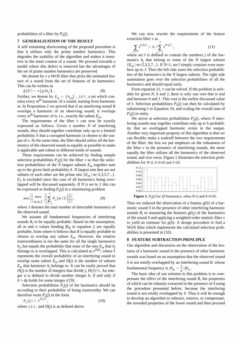
probabilities of a filter byPs(j).
7 GENERALIZATION OF THE RESULTA still remaining shortcoming of the proposed procedure isthat it utilizes only the prime number harmonics. Thisdegrades the usability of the algorithm and makes it sensi-tive to the tonal content of a sound. We proceed towards amodel where this defect is removed but the advantages ofthe set of prime number harmonics are preserved.
We denote byv a WOS filter that picks the estimated fea-ture of a sound from the set of features of its harmonics.This can be written as
. (8)
Further, we denote by , , a set which con-tains everymth harmonic of a sound, starting from harmonicm. In Proposition2 we proved that if an interfering soundRoverlaps a harmonic of an observing sound, it overlapseverymth harmonic of it, i.e., exactly the subsetEm.
The requirements of the filterv can now be exactlyexpressed as follows. Given a numberN of interferingsounds, they should together contribute only up to a limitedprobabilityλ that a corrupted harmonic is chosen to the out-put ofv. At the same time, the filter should utilize all the har-monics of the observed sound as equally as possible to makeit applicable and robust to different kinds of sounds.
These requirements can be achieved by finding sampleselection probabilitiesPs(j) for the filterv so that the selec-tion probabilities of theN largest subsetsEm together sumup to the given limit probabilityλ. N largest sets that are notsubsets of each other are the prime sets {Em | m=2,3,5,7...}.E1 is excluded since the case of all harmonics being over-lapped will be discussed separately. If N is set to 1 this canbe expressed as findingPs(j) in a minimizing problem
, (9)
whereJ denotes the total number of detectable harmonics ofthe observed sound.
We assume all fundamental frequencies of interferingsoundsRi to be equally probable. Based on the assumption,all m and n values bindingf0R in equation 2 are equallyprobable, from where it follows thatR is equally probable tochoose to overlap any subsetEm. However, the relativetrustworthiness is not the same for all the single harmonicshj, but equals the probability that none of the setsEm thathjbelongs to is overlapped. This is calculated asτD(j), whereτrepresents the overall probability of an interfering sound tooverlap some subsetEm andD(j) is the number of subsetsEm that harmonichj belongs to. It can be easily proved thatD(j) is the number of integers that dividej, D(1)=1. An inte-ger a is defined todivide another integerb, if and only ifb = da holds for some integerd [9].
Selection probabilitiesPs(j) of the harmonics should beaccording to their probability of being trustworthy. We cantherefore writePs(j) in the form
, (10)
where , andD(j) is as defined above.
g S( ) v g hj( ){ }=
Em hmj{ }= j 1≥
min max
m 2≥Ps m i⋅( )
i 1=
J
∑
Ps j( ) τD j( )=
j 1≥
We can now rewrite the requirements of the featureexraction filterv as
, (11)
where setI is defined to contain the numbersj of the har-monics hj that belong to some of theN largest subsets{ Em | m=2,3,5,7...}. IfN=1, setI simply contains even num-bers up toJ. Thus the left side sums the selection probabili-ties of the harmonics in theN largest subsets. The right sidesummation goes over the selection probabilities of all theharmonics and should equal unity.
From equation 11, τ can be solved. If the problem is solv-able for givenN, λ andJ, there is only one root that is realand between 0 and 1. This root is the earlier discussed valueof τ. Selection probabilitiesPs(j) can then be calculated bysubstitutingτ to Equation 10, and scaling the overall sum ofPs(j) to unity.
We arrive at selection probabilitiesPs(j), whereN inter-fering sounds may together contribute only up toλ probabil-ity that an overlapped harmonic exists in the output.Another very important property of this algorithm is that wecan flexibly make a tradeoff between the two requirementsof the filter: the less we put emphasis on the robustness ofthe filter v in the presence of interfering sounds, the moreequally the filter utilizes all the harmonics of the observedsound, and vice versa. Figure 1 illustrates the selection prob-abilities forN=2, λ=0.45 andJ=20.
Thus we reduced the observation of a featureg(S) of a har-monic soundS in the presence of other interfering harmonicsoundsRi to measuring the featuresg(hj) of the harmonicsof the soundS and applying a weighted order statistic filtervto yield an estimate forg(S). A design procedure to find aWOS filter whichimplements the calculated selection prob-abilites is presented in [10].
8 FEATURE SUBTRACTION PRINCIPLEOur algorithm and discussion on the observation of the fea-
tures of a harmonic sound in the presence of other harmonic
sounds was based on an assumption that the observed sound
S is not totally overlapped by an interfering sound R, whose
fundamental frequency is .
The basic idea of our solution to this problem is tocom-pensate the effect of the interfering soundR, the propertiesof which can be robustly extracted in the presence ofS usingthe procedure presented before, because the interferingsound is not totally overlapped byS. Thus it will be enoughto develop an algorithm to subtract, remove, or compensate,the revealed properties of the lower sound and then proceed
τD j( )
j I∈∑ λ τD j( )
j 1=
J
∑⋅=
0 2 4 6 8 10 12 14 16 18 200
0.02
0.04
0.06
0.08
0.1
0.12
Figure 1. Ps(j) for 20 harmonics, whenN=2 andλ=0.45.
0.120.100.080.060.040.020.00
f0R1n--- f0S⋅=

to determine the properties of the soundS, which is laid barefrom under the interfering sound. The subtraction processdepends on the feature under inspection, and cannot be pre-sented in a general form.
9 ALGORITHM EVALUATIONOur algorithm was evaluated and verified by applying it in acomputer program whose purpose is to transcribe poly-phonic piano music. The program is first allowed to studypiano notes one by one, a sufficient amount to represent allthe different tone colours that can be produced by thatinstrument. After this we require the program to transcriberich polyphonic musical signals played with the same instru-ment, i.e., to determine the fundamental frequencies and theloudnesses of the sounds in the signals.
In all test cases, the transcription was done withoutknowledge of the polyphony of the transcribed signals, andwith a fixed constant set of parameters. The range of funda-mental frequencies was restricted to extend from 65Hz to2100Hz, where five octaves and 61 piano keys fit inbetween. An acoustic upright piano was used in simulations.
Transcription proceeds by first detecting all potential notecandidates in the spectrum, and then resolving their loud-nesses one by one, using the new method. Naturally, thereare much more potential note candidates than truly playednotes. We call true notes the notes that were truly played inthe recorded signals, andfalse notes those that appear asnote candidates, although they were not actually played.
The goodness of the algorithm is justified by its ability toindicate the truly existing sound in the signal, i.e. the loud-ness of the true notes should raise clearly above the loudnessof the false ones. The loudnesses of the candidates in eachtime segment are scaled between the values 0 to 100.
Certain note combinations were separately played andfed to the transcriber to review its ability to resolve richmusical polyphonies. Results are presented in Table 1. In thefirst type of tests, consonant and dissonant chords wereplayed, two in each of the five octaves. In the second test,groups of adjacent notes in the piano keyboard were playedin each octave. Third, groups of seven random notes wereallotted in the allowed range of pitces and played. In each ofthese tests, average loudnesses among the true and falsenotes were calculated and recorded. Also the worst cases,where the loudness of the false notes gets closest to the truenotes, was recorded. The polyphony, number of notes ineach test, is also indicated.
Chosen classical compositions were played and excerptsfrom them were posed to our transcription system to test itspractical transcription efficiency. Here we used 25% relative
Table 1: Relative loudnesses of the true and false notes.
Test typePolyp.Averages Worst case
min true max false min true max falsechords 3-4 64 17 78 43groups 4-5 48 7 30 7random 7 21 11 10 11
loudness as a threshold to segregate between true and falsenotes. Weaker candidates were discarded as false notes.Results are presented in Table 2. The last piece was playedby a computer on an electric piano. The effect of all noteshaving roughly equal playing loudness and the absence ofcross resonance and noise can be noticed in the results.
Finding the exact fundamental frequencies of the sounds inthe analyzed signals proved successful in all cases. Theywere not assumed to be quantized to the closest legal notes.
10 CONCLUSIONThe problem of resolving rich musical polyphonies was themotivation for developing the new methods. Simulationsillustrate that the current system works within certain errorlimits up to seven notes polyphony. Especially, althoughincrease in polyphony brings the levels of the weakest truenote and the strongest false note closer to each other, thesystem does not totally break down even in rich polypho-nies. We conclude that a number theoretical analysis of asound mixture is the key to a robust detection and observionof harmonic sounds in the interference of each other.
REFERENCES[1] Kashino, Nakadai, Kinoshita, Tanaka. “Application of
Bayesian probability network to music scene analysis”.Proceedings of the Int. Joint Conference on ArtificialIntelligence, CASA workshop, 1995
[2] Martin. “A Blackboard System for Automatic Transcrip-tion of Simple Polyphonic Music”. MIT Media Labora-tory Perceptual Computing Section Technical ReportNo. 399, 1996.
[3] McAulay, Quatieri. “Speech analysis/synthesis based ona sinusoidal representation”.IEEE Trans. ASSP, 34(4),pp. 744-754, 1986.
[4] Depalle, García, Rodet. “Tracking of Partials for Addi-tive Sound Synthesis Using Hidden Markov Models”.IEEE Trans. on ASSP, 1993.
[5] Serra. “Musical Sound Modeling With Sinusoids PlusNoise”. Roads, Pope, Poli (eds.). “Musical SignalProcessing”. Swets & Zeitlinger Publishers, 1997.
[6] Astola, Kuosmanen. “Fundamentals of Nonlinear DigitalFiltering”. CRC Press LLC, 1997.
[7] Kuosmanen. “Statistical Analysis and Optimization ofStack Filters”. Tech.D. thesis., Acta Polytechnica Scan-dinavia, Electrical Engineering Series, 1994.
[8] Koblitz. “A Course in Number Theory and Cryptogra-phy”. Springer, Berlin, 1987.
[9] Klapuri. “Automatic Transcription of Music”. MSc the-sis, Tampere University of Technology, 1998.
Table 2: Transcription results using 25% loudness limit.
Composition Notesin total
Typicalpolyphony
Missingnotes
Erroneousextra notes
Für Elise, I 86 1 - 3Für Elise, II 190 half:2 half:4 9 6Inventio 8 205 2 15 4
Rondo alla Turca 142 3 (up to 5) 1 -

Publication 2
A. P. Klapuri, “Sound onset detection by applying psychoacoustic knowledge,” In Proc. IEEEInternational Conference on Acoustics, Speech, and Signal Processing, Phoenix, Arizona,1999.
© 2004 IEEE. Reprinted, with permission, from Proc. IEEE International Conference onAcoustics, Speech, and Signal Processing 1999.
Personal use of this material is permitted. However, permission to reprint/republish this material for creating newcollective works or for resale or redistribution to servers or lists or to reuse any copyrighted component of thiswork in other works must be obtained from the IEEE.


ABSTRACT
A system was designed, which is able to detect the perceptualonsets of sounds in acoustic signals. The system is general inregard to the sounds involved and was found to be robust for dif-ferent kinds of signals. This was achieved without assuming regu-larities in the positions of the onsets. In this paper, a method isfirst proposed that can determine the beginnings of sounds thatexhibit onset imperfections, i.e., the amplitude envelope of whichdoes not rise monotonically. Then the mentioned system isdescribed, which utilizes band-wise processing and a psychoa-coustic model of intensity coding to combine the results from theseparate frequency bands. The performance of the system wasvalidated by applying it to the detection of onsets in musical sig-nals that ranged from rock to classical and big band recordings.
1. INTRODUCTION
Onset detection plays an important role in the computational seg-mentation and analysis of acoustic signals. It greatly facilitatescut-and-paste operations and editing of audio recordings. Theonset information may also be used in audio/video synchroniza-tion and timing, or passed for further analysis and recognition forexample in an acoustic supervision system.
We use the termonset detection to refer to the detection of thebeginnings of discrete events in acoustic signals. A percept of anonset is caused by a noticeable change in the intensity, pitch ortimbre of the sound [1]. A fundamental problem in the design ofan onset detection system is distinguishing genuine onsets fromgradual changes and modulations that take place during the ring-ing of a sound. This is also the reason why robust one-by-onedetection of onsets has proved to be very hard to attain withoutsignificantly limiting the set of application signals.
A lot of research related to onset detection has been carried out inrecent years. However, only few systems have set out to solve theproblem of one-by-one onset detection [1][2][3]. Instead, mostsystems aim at higher-level information, such as the perceivedbeat of a musical signal [4][5][6], in which case long-term auto-correlations and regularities can be used to remove single errorsand to tune the sensitivity of the low-level detection process.
In this paper, we first propose a mathematical method to copewith sounds that exhibit onset imperfections, i.e., the amplitudeenvelope of which rises through a complex track and easily pro-duces erroneous extra onsets or an incorrect time value. Then wepropose the application of psychoacoustic models of intensitycoding, which enable us to determine system parameters that
apply to a wide variety of input signals. This allows processingthem without a priori knowledge of signal contents or separatetuning of parameters.
The realized system was validated by applying it to the detectionof onsets in musical signals. This was done mainly for two rea-sons. First, musical signals introduce a rich variety of sounds witha wide range of pitches, timbres and loudnesses. Different combi-nations of onsetting and backgrounding sounds are readily availa-ble. Second, verifying the contents of a musical signal issomewhat easier than in the case of environmental sounds. Alsothe concept of a perceivable onset is better defined. It should benoted, however, that the algorithm is not limited to musical sig-nals, because the regularities and rhythmic properties of musicalsignals are not utilized in the detection process. The system per-forms reliably for input signals that ranged from rock music toclassical and big band recordings, both with and without drums.
2. SYSTEM OVERVIEW
The earliest onset detection systems typically tried to process theamplitude envelope of a signal as a whole (see e.g. [7]). Since thiswas not very effective, later proposals have evolved towardsband-wise processing. Scheirer was the first to clearly point outthe fact that an onset detection algorithm should follow thehuman auditory system by treating frequency bands separatelyand then combining results in the end [4]. An earlier system ofBilmes’s was on the way to the same direction, but his systemonly used a high-frequency and a low-frequency band, which wasnot that effective[2].
Scheirer describes a psychoacoustic demonstration on beat per-ception, which shows that certain kinds of signal simplificationscan be performed without affecting the perceived rhythmic con-tent of a musical signal [4]. When the signal is divided into atleast four frequency bands and the corresponding bands of a noisesignal are controlled by the amplitude envelopes of the musicalsignal, the noise signal will have a rhythmic percept which is sig-nificantly the same as that of the original signal. On the otherhand, this does not hold if only one band is used, in which casethe original signal is no more recognizable from its simplifiedform.
The overview of our onset detection system is presented inFigure1. It utilizes the band-wise processing principle as moti-vated above. First, the overall loudness of the signal is normalizedto 70dB level using the model of loudness as proposed by Mooreet al. [8]. Then a filterbank divides the signal into 21 non-overlap-ping bands. At each band, we detectonset components and deter-mine their time and intensity. In final phase, the onset components
SOUND ONSET DETECTION BY APPLYINGPSYCHOACOUSTIC KNOWLEDGE
Anssi Klapuri
Signal Processing Laboratory, Tampere University of TechnologyP.O.Box 553, FIN-33101 Tampere, FINLAND

are combined to yield onsets.
Since we use psychoacoustic models both in onset componentdetection, in its time and intensity determination, and in combin-ing the results, it is important to use a filterbank which can pro-vide input to the models. Therefore, we choose a bank of nearlycritical-band filters which covers the frequencies from 44Hz to18kHz. The lowest three among the required 21 filters are one-octave band-pass filters. The remaining eighteen are third-octaveband-pass filters. All subsequent calculations can be done oneband at a time. This reduces the memory requirements of thealgorithm in the case of long input signals, assumed that parallelprocessing is not desired.
The output of each filter is full-wave rectified and then decimatedby factor 180 to ease the following computations. Amplitudeenvelopes are calculated by convolving the band-limited signalswith a 100ms half-Hanning (raised cosine) window. This windowperforms much the same energy integration as the human auditorysystem, preserving sudden changes, but masking rapid modula-tion [9][4].
3. CALCULATION OF ONSET COMPONENTS
3.1 Onset Component Detection
Several algorithms for picking potential onset candidates from anamplitude envelope function have been presented in the literature[5][6][2][4]. Despite the number of variants, practically all ofthem are based on the calculation of a first order difference func-tion of the signal amplitude envelopes and taking the maximumrising slope as an onset or an onset component.
In our simulations, it turned out that the first order differencefunction reflects well the loudness of an onsetting sound, but itsmaximum values fail to precisely mark the time of an onset. Thisis due to two reasons. First, especially low sounds may take sometime to come to the point where their amplitude is maximally ris-ing, and thus that point is crucially late from the physical onset ofa sound and leads to an incorrect cross-band association with thehigher frequencies. Second, the onset track of a sound is mostoften not monotonically increasing, and thus we would have sev-
onsetcompo-nents
source onsets
1
2
21
Scalesignal
level to70dB
Combineresultsto yieldonsets
Band-wiseprocessing
(see Fig. 1b)
Figure 1a. System overview.
Amplitudeenvelopeextraction
Onsetcomponentdetection
Determinecomponent’s
time andintensity
Figure 1b. Processing at each frequency band.
Filterbank
eral local maxima in the first order difference function near thephysical onset (see plots with a dashed line in Figure 2).
We took an approach that effectively handles both of these prob-lems. We begin by calculating a first order difference function
,
whereA(t) denotes the amplitude envelope function.D(t) is set tozero where signal is below minimum audible field. Then wedivide the first order difference function by the amplitude enve-lope function to get a first order relative difference function W,i.e., the amount of change in relation to the signal level. This is thesame as differentiating the logarithm of the amplitude envelope.
We use the relative difference functionW(t) both to detect onsetcomponents and to determine their time. This is psychoacousti-cally relevant, since perceived increase in signal amplitude is inrelation to its level, the same amount of increase being moreprominent in a quiet signal. According to Moore, the smallestdetectable change in intensity is approximately proportional to theintensity of the signal[10]. That is,∆I / I, the Weber fraction, is aconstant. This relationship holds for intensities from about 20dBto about 100dB above the absolute threshold. The function
is equivalent toW(t), since the frequencyf in is reduced in the division. Thus we detect onset
components by a simple peak picking operation, which looks forpeaks above a global thresholdTdet in the relative difference func-tion W(t).
The relative difference function effectively solves the abovemen-tioned problems by detecting the onset times of low sounds ear-lier and, more importantly, by handling complicated onset tracks,since oscillations in the onset track of a sound do not matter inrelative terms after its amplitude has started rising. To clarify this,we plotted the absolute and relative difference functions of theonset of a piano sound in Figure 2. Both of the benefits discussedcan be seen clearly.
3.2 Intensity of an Onset Component
Simultaneously occurring sounds combine by a linear summation.In determining the intensity of an already detected onset compo-nent, we can assume the level of backgrounding sounds to be
330 340 350 360 370 380 390 400 410 420 4300
1
2
3
4
5
6
Dashed line:
(A(t))
Solid line:
(log(A(t)))
whereA(t) denotesthe amplitude enve-lope function.
ddt-----
ddt-----
6
5
4
3
2
1
Figure 2. Onset of a piano sound. First orderabsolute(dashed) andrelative (solid) difference functions of theamplitude envelopes of six different frequency bands.
D t( ) ddt----- A t( )( )=
W t( ) ddt----- A t( )( )log( )=
∆I t( ) I t( )⁄I t( ) A t( ) f⋅=

momentarily steady and take the increase in level to be due to theonsetting sound(s). Thus the asked intensity can be picked fromthe first order difference functionD(t), multiplied by the bandcenter frequencyfB. The intensity is needed later when onsetcomponents are combined to yield onsets of the overall signal.
An appropriate point in time to pick the intensity fromD(t) is notas early as where the onset was determined to occur. Instead, wescan forward up to the point where amplitude envelope startsdecreasing and determine the intensity at the point of maximumslope, i.e., at the maximum value ofD(t) between the onset andthe point where amplitude stops increasing.
After intensities has been determined for all onset components atthe band, we check them through and drop out components thatare closer than 50ms to a more intense component. Remainingones are accepted.
4. COMBINING THE RESULTS FROM THE BANDS
In the final phase we combine onset components from separatebands to yield onsets of the overall signal. For this purpose, weimplemented the model of loudness as proposed by Moore, Glas-berg and Baer [8]. Input to our implementation is a vector ofsound intensities at third-octave bands between 44Hz and18kHz, from which the program calculates the loudness of thesignal in phons. To optimize the computational efficiency of theprocedure, we slightly simplified the model by making the shapeof the excitation pattern, i.e., the intensity spread between adja-cent critical bands independent from sound pressure level. Thisaccelerated the computations remarkably, but did not make a sig-nificant difference to the estimated loudness values for the soundintensity levels we are using.
The onsets of the overall signal are calculated as follows. First theonset components from different bands are all sorted in timeorder, and are regarded as sound onset candidates hereafter. Theneach onset candidate is assigned a loudness value, which is calcu-lated by collecting onset components in a 50ms time windowaround the candidate and feeding their intensities to the corre-sponding frequency bands of the loudness model of Moore et al.Since most candidates have only a couple of contributing onsetcomponents at different bands, we must use minimum level, orbackground noise level for the other bands in the input of themodel. Repeating this procedure to each onset candidate yields avector of candidate loudnesses as a function of their times, asillustrated in Figure3 for a popular music signal.
Onset loudnesses that were estimated using the abovementinedprocedure corresponded very well to the perceived loudnesses ofthe onsets in verificative listening tests. It turned out that a robustdetection of onsets in very diverse kinds of signals can now beachieved by a simple peak picking operation, which looks foronset candidates above a global threshold valueTfinal. We dropout onset candidates whose loudness falls below the threshold.Then we also drop out candidates that are too close (50ms) to alouder candidate. Among equally loud but too close candidates,the middle one (median) is chosen and the others are abandoned.The remaining onset candidates are accepted as true ones. A goodvalue forTfinal was found to be 25dB for signals, whose averageloudnesses had been normalized to 70dB level.
5. VALIDATION EXPERIMENTS
The presented procedure was verified by testing its performancein detecting onsets in musical signals. The signals were selectedto comprise a large variation of musical instruments and a widedynamic and pitch range. Signals both with and without drumswere included. Another goal was to include representativeexcerpts from different musical genres, ranging from jazz androck to classical and big band music.
Approximately ten second excerpts were sampled from each per-formance. These periods were carefully inspected and their onsettimes were marked. The excerpts were then feeded to the onsetdetection system and its results were compared to the manualtranscription. All simulation cases were computed using the verysame set of parameter values and thresholds, without separate tai-loring for each simulation case. The algorithm itself was asexplained above. Higher-level rhythmic properties and regulari-ties of musical signals were not utilized in the detection.
It is interesting to note that the limitations of our detection systemresemble those of human perception. We define apseudo-onset tobe a sound beginning, which undisputably exists in a signal, butcannot be detected by a human listener if the signal is not pre-sented in short segments and several times. Since objective listen-ing test could not be arranged, we regard undetected pseudo-onsetas errors, too. It turned out that the detection of some pseudo-onsets could not be achieved without giving rise to several erro-neous extra onsets that are due to gradual changes and modula-tions during the ringing of sounds.
Onset detection results for ten different musical signals are sum-marized in Table 1. The total number of onsets, number of unde-tected onsets and the number of erroneous extra onsets are given.A measure of correctness in the rightmost column is calculated as
%.
A more detailed discussion of each case follows.
Chopin’s classical piano etude (op. 25, no. 4) was a trivial case.Still three onsets fell below threshold because the notes were lowpitched, played softly and masked by other notes.Al Di Meola’s‘Orient Blue’ represents a much more difficult case. The piece ispolyphonic and employs the whole dynamic and pitch range ofthe acoustic guitar. Shortest inter-note intervals are only a fif-teenth of a second. Good results were achieved partly because of
0 0.5 1 1.5 2 2.5
x 105
10
15
20
25
30
35
40
45
50
55/share/SpeechDat/klap/grusin01.wav : 1..220000
loudness (dB)
45
40
35
30
25
20
Figure 3. The loudness of onsets as a function of their time.The genuine onsets can now be quite easily discerned.
cor recttotal undetected– extra–
total------------------------------------------------------------------- 100⋅=
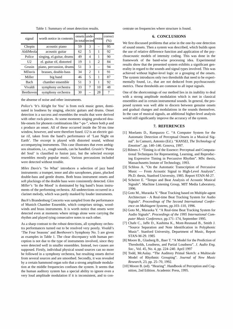
the absense of noise and other instruments.
Police’s ‘It’s Alright for You’ is from rock music genre, domi-nated in loudness by singing, electric guitars and drums. Onsetdetection is a success and resembles the results that were derivedwith other rock-pieces. At some moments singing produced dou-ble-onsets for phonem combinations like “-ps-”, where bothp ands produce an onset. All of these occurred inside the 50ms timewindow, however, and were therefore fused.U2 is an electric gui-tar rif, taken from the band’s performance of ‘Last Night onEarth’. The excerpt is played with distorted sound, withoutaccompanying instruments. This case illustrates that even ambig-uos situations, i.e., rough sounds, can be handled.Grusin’s ‘Puntadel Soul’ is classified to fusion jazz, but the selected excerptresembles mostly popular music. Various percussions includedwere detected without trouble.
Miles Davis’s ‘So What’ introduces a selection of jazz bandinstruments: a trumpet, tenor and alto saxophones, piano, pluckeddouble-bass and gentle drums. Both brass instrument onsets andsoft pluckings of the double bass were consistently detected.GlenMiller’s ‘In the Mood’ is dominated by big band’s brass instru-ments of the performing orchestra. All undetections occurred in aclarinet melody, which was partly masked by louder instruments.
Bach’s Brandenburg Concerto was sampled from the performanceof Munich Chamber Ensemble, which comprises strings, wood-winds and brass instruments. It is worth notice that onsets weredetected even at moments where strings alone were carrying therhythm and played tying consecutive notes to each other.
As a sharp contrast to the robust detections, all symphony orches-tra performances turned out to be resolved very poorly. Vivaldi’s‘The Four Seasons’ andBeethoven’s Symphony No. 5 are givenas examples in Table 1. The clear discrepancy with human per-ception is not due to the type of instruments involved, since theywere detected well in smaller ensembles. Instead, two causes aresupposed. Firstly, individual physical sound sources can no morebe followed in a symphony orchestra, but resulting onsets derivefrom several sources and are smoothed. Secondly, it was revealedby a certain hammond organ solo that a strong amplitude modula-tion at the middle frequencies confuses the system. It seems thatthe human auditory system has a special ability to ignore even avery loud amplitude modulation if it is inconsistent, and to con-
Table 1: Summary of onset detection results.
signal worth notice in contentsonsetsin total
unde-tected
extracorrect
(%)
Chopin acoustic piano 59 3 – 95
AldiMeola acoustic guitar 62 5 1 92
Police singing, el.guitar, drums 49 4 1 90
U2 el. guitar rif, distorted 19 1 2 84
Grusin piano, percussion, drums51 3 – 94
MDavis brasses, double-bass 34 2 1 91
Miller big band 46 5 1 87
Bach chamber ensemble 51 3 1 92
Vivaldi symphony orchestra 33 7 10 48
Beethoven symphony orchestra 30 – 28 7
centrate on frequencies where structure is found.
6. CONCLUSIONS
We first discussed problems that arise in the one-by-one detectionof sound onsets. Then a system was described, which builds uponthe use of relative difference function and application of the psy-choacoustic models of intensity coding. This was done in theframework of the band-wise processing idea. Experimentalresults show that the presented system exhibits a significant gen-erality in regard to the sounds and signal types involved. This wasachieved without higher-level logic or a grouping of the onsets.The system introduces only two thresholds that need to be experi-mentally found, i.e., that are not deduced from psychoacousticmetrics. These thresholds are common to all input signals.
One of the shortcomings of our method lies in its inability to dealwith a strong amplitude modulation which is met in classicalensembles and in certain instrumental sounds. In general, the pro-posed system was well able to discern between genuine onsetsand gradual changes and modulations in the sounds themselves.In the case of musical signals, an additional higher-level analysiswould still significantly improve the accuracy of the system.
7. REFERENCES
[1] Moelants D., Rampazzo C. “A Computer System for theAutomatic Detection of Perceptual Onsets in a Musical Sig-nal”. In Camurri, Antonio (Ed.). “KANSEI, The Technology ofEmotion”, pp. 140–146. Genova, 1997.
[2] Bilmes J. “Timing is of the Essence: Perceptual and Computa-tional Techniques for Representing, Learning, and Reproduc-ing Expressive Timing in Percussive Rhythm”. MSc thesis,Massachusetts Instute of Technology, 1993.
[3] Schloss A. ”On the Automatic Transcription of PercussiveMusic — From Acoustic Signal to High-Level Analysis”.Ph.D. thesis, Stanford University, 1985. Report STAN-M-27.
[4] Scheirer E. “Tempo and Beat Analysis of Acoustic MusicalSignals”. Machine Listening Group, MIT Media Laboratory,1996.
[5] Goto M., Muraoka Y. “Beat Tracking based on Multiple-agentArchitecture - A Real-time Beat Tracking System for AudioSignals”. Proceedings of The Second International Confer-ence on Multiagent Systems, pp.103–110, 1996.
[6] Goto M., Muraoka Y. “A Real-time Beat Tracking System forAudio Signals”.Proceedings of the 1995 International Com-puter Music Conference, pp.171–174, September 1995.
[7] Chafe C., Jaffe D., Kashima K., Mont-Reunaud B., Smith J.“Source Separation and Note Identification in PolyphonicMusic”. Stanford University, Department of Music, ReportSTAN-M-29. 1985
[8] Moore B., Glasberg B., Baer T. “A Model for the Prediction ofThresholds, Loudness, and Partial Loudness”.J. Audio Eng.Soc., Vol. 45, No. 4, pp. 224–240. April 1997
[9] Todd, McAulay. “The Auditory Primal Sketch: a MultiscaleModel of Rhythmic Grouping”.Journal of New MusicResearch, 23, pp. 25–70, 1992.
[10] Moore B. (ed). “Hearing”. Handbook of Perception and Cog-nition, 2nd Edition. Academic Press, 1995.

Publication 3
A. P. Klapuri, “Multipitch estimation and sound separation by the spectral smoothness princi-ple,” In Proc. IEEE International Conference on Acoustics, Speech, and Signal Processing,Salt Lake City, Utah, 2001.
© 2004 IEEE. Reprinted, with permission, from Proc. IEEE International Conference onAcoustics, Speech, and Signal Processing 2001.
Personal use of this material is permitted. However, permission to reprint/republish this material for creating newcollective works or for resale or redistribution to servers or lists or to reuse any copyrighted component of thiswork in other works must be obtained from the IEEE.

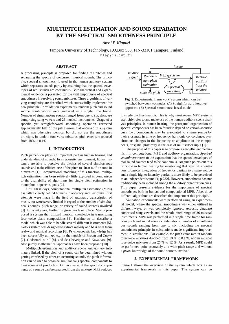
MULTIPITCH ESTIMATION AND SOUND SEPARATIONBY THE SPECTRAL SMOOTHNESS PRINCIPLE
Anssi P. Klapuri
Tampere University of Technology, P.O.Box 553, FIN-33101 Tampere, [email protected]
sal-of
ustice byyn-o-
ha-
ofthish-rcednots.
tralree.n-in
secaln-ne-ale-maldut
anbe
ABSTRACT
A processing principle is proposed for finding the pitches andseparating the spectra of concurrent musical sounds. The princi-ple, spectral smoothness, is used in the human auditory systemwhich separates sounds partly by assuming that the spectral enve-lopes of real sounds are continuous. Both theoretical and experi-mental evidence is presented for the vital importance of spectralsmoothness in resolving sound mixtures. Three algorithms of var-ying complexity are described which successfully implement thenew principle. In validation experiments, random pitch and soundsource combinations were analyzed in a single time frame.Number of simultaneous sounds ranged from one to six, databasecomprising sung vowels and 26 musical instruments. Usage of aspecific yet straightforward smoothing operation correctedapproximately half of the pitch errors that occurred in a systemwhich was otherwise identical but did not use the smoothnessprinciple. In random four-voice mixtures, pitch error rate reducedfrom 18% to 8.1%.
1. INTRODUCTION
Pitch perception plays an important part in human hearing andunderstanding of sounds. In an acoustic environment, human lis-teners are able to perceive the pitches of several simultaneoussounds and make efficient use of the pitch to “hear out” a sound ina mixture [1]. Computational modeling of this function, multip-itch estimation, has been relatively little explored in comparisonto the availability of algorithms for single pitch estimation inmonophonic speech signals [2].
Until these days, computational multipitch estimation (MPE)has fallen clearly behind humans in accuracy and flexibility. Firstattempts were made in the field of automatic transcription ofmusic, but were severy limited in regard to the number of simulta-neous sounds, pitch range, or variety of sound sources involved[3]. In recent years, further progress has taken place. Martin pro-posed a system that utilized musical knowledge in transcribingfour voice piano compositions [4]. Kashinoet al. describe amodel which was able to handle several different instruments [5].Goto’s system was designed to extract melody and bass lines fromreal-world musical recordings [6]. Psychoacoustic knowledge hasbeen succesfully utilized e.g. in the models of Brown and Cooke[7], Godsmarket al. [8], and de Cheveigne and Kawahara [9].Also purely mathematical approaches have been proposed [10].
Multipitch estimation and auditory scene analysis are inti-mately linked. If the pitch of a sound can be determined withoutgetting confused by other co-occurring sounds, the pitch informa-tion can be used to organize simultaneous spectral components totheir sources of production. Or, vice versa, if the spectral compo-nents of a source can be separated from the mixture, MPE reduces
to single pitch estimation. This is why most recent MPE systemexplicitly refer to and make use of the human auditory scene anysis principles. In human hearing, the perceptual organizationspectral components has been found to depend on certain acocues. Two components may be associated to a same sourctheir closeness in time or frequency, harmonic concordance, schronous changes in the frequency or amplitude of the compnents, or spatial proximity in the case of multisensor input [1].
The purpose of this paper is to propose a new efficient mecnism in computational MPE and auditory organization.Spectralsmoothnessrefers to the expectation that the spectral envelopesreal sound sources tend to be continuous. Bregman points outprinciple in human hearing by mentioning that spectral smootness promotes integration of frequency partials to a same souand a single higher intensity partial is more likely to be perceiveas an independent sound [1, p.232]. However, smoothness hastraditionally been included among the auditory organization cueThis paper presents evidence for the importance of specsmoothness both in human and computational MPE. Also, thdifferent algorithms are described that implement this principle
Validation experiments were performed using an experimetal model, where the spectral smoothness was either utilizeddifferent ways, or was completely ignored. Acoustic databacomprised sung vowels and the whole pitch range of 26 musiinstruments. MPE was performed in a single time frame for radom pitch and sound source combinations, number of simultaous sounds ranging from one to six. Including the spectrsmoothness principle in calculations made significant improvment in simulations. For example, the pitch error rate in randofour-voice mixtures dropped from 18 % to 8.1 %, and in musicfour-voice mixtures from 25 % to 12 %. As a result, MPE coulbe performed quite accurately at a wide pitch range and withoa priori knowledge of the sound sources involved.
2. EXPERIMENTAL FRAMEWORK
Figure 1 shows the overview of the system which acts asexperimental framework in this paper. The system can
F, β, spectrummixturesignal Remove
partialsfrom themixture
iterate
store the pitch
Spectralsmoothing
Predomi-nant pitchestimation
Fig. 1.Experimental framework: system which can beswitched between two modes. (A) Straightforward iterativeapproach. (B) Spectral-smoothness based model.
A
B

y
is
oon
lsofre,ove
ls
om-o-
izedt
te-in
so,
si-aylly
nda-entis
e,
switched between two modes. The straightforward iterative MPEmodel, denoted by branchA, has been described earlier in [11]. Itconsists of two main parts that are applied in an iterative succes-sion. The first part, predominant pitch estimation, finds the pitchof the most prominent sound in the interference of other harmonicand noisy sounds. As an output, it gives the fundamental fre-quencyF, inharmonicity factorβ, and the precise frequencies andamplitudes of the harmonic partials of the sound. In the secondpart, the spectrum of the detected sound is linearly subtractedfrom the mixture. These are then repeated for the residual signal.
A spectral-smoothness based model is obtained by locating anadditional module between the estimation and subtraction stages.This is denoted by branchB in Fig. 1. The aim of the spectralsmoothing algorithm is to use the pitch information to produce amore appropriate estimate for the spectrum of a separated soundbefore it is subtracted from the mixture. The need for such a mod-ule is strongly motivated by two observations. The predominantpitch estimation algorithm is capable of finding one of the correctpitches with 99 % certainty even in six-voice polyphonies [11].However, the probability of error increases rapidly in the courseof iteration. This indicates that the initial estimate of a soundspectrum as given by predominant pitch algorithm is not accurateenough to remove it correctly from the mixture.
3. DIAGNOSIS OF THE STRAIGHTFORWARDITERATIVE SYSTEM
Simulations were run to analyze the behaviour of the straightfor-ward iterative estimation and separation approach, i.e., the branchA in Figure 1. Random mixtures ofN sounds were generated byfirst allotting an instrument and then a random note from itswhole playing range, however, restricting the pitch over fiveoctaves between 65 Hz and 2100 Hz. The desired number ofsounds was allotted, and them mixed with equal mean square lev-els. The iterative process was then evoked and requested to extractN pitches from the acoustic mixture signal. As a general impres-sion, the presented iterative approach works rather reliably.
However, an important observation is immediately madewhen the distribution of the remaining errors is analyzed. Figure 2shows the errors as a function of the musical intervals that occurin the erroneously transcribed sound mixtures. It appears that theerror rate is strongly correlated with certain pitch relations. Moreexactly, the straightforward estimation and subtraction approachis likely to fail in cases where the fundamental frequencies ofsimultaneous sounds are in simple rational number relations, alsocalled harmonic relations. These are indicated over the corre-sponding bars in Fig. 2.
3.1 Coinciding sinusoidal partials
It turned out that coinciding frequency partials from differentsounds make the algorithm fail. If sounds are in a harmonic rela-tion to each other, a lot of partials coincide, i.e., share the samefrequency. When the firstly detected sound is removed, the coin-ciding harmonics of remaining sounds are also removed in thesubtraction procedure. In some cases, and particularly after sev-eral iterations, a remaining sound gets too corrupted to be cor-rectly analyzed in the coming iterations.
When two sinusoidal partials with amplitudesa1 anda2 and
phase differenceθ∆ coincide in frequency, the amplitude of theresulting sinusoid can be calculated as
. (1)
If the two amplitudes are roughly equivalent, the partials maeither amplify or cancel each other, depending onθ∆. However, ifone of the amplitudes is significantly larger than the other, asusually the case,asapproaches the maximum of the two.
3.2 Fundamental frequency relations
The condition that a harmonic partialh of a soundS coincides aharmonicj of another soundR can be written as ,whereFS and FR are the fundamental frequencies, and the twsides represent the frequencies of the partials. When the commfactors of integersh andj are reduced, this yields
, (2)
where are integer numbers. This implies that partiaof two sounds can coincide only if the fundamental frequenciesthe two sounds are in rational number relations. Furthermowhen the fundamental frequencies of two sounds are in the abrelation, then everymth harmonicmk of the soundS coincideseverynth harmonicnk of the soundR at their common frequencybands, where integer . This is evident since equa
for each pairh=mk andj=nk, when Eq. (2) holds.An important principle governing music is paying attention t
the pitch relations, intervals, of simultaneously played notes. Siple harmonic relations satistying Eq. (2) are favoured over dissnant ones. Although western music arranges notes to a quantlogarithmic scale, it can surprisingly well produce the differenharmonic intervals that can be derived by substituting small ingers to Eq. (2) [3]. Because harmonic relations are so commonmusic, these “worst cases” must be handled well in general. Althis explains why MPE is particularly difficult in music.
4. SOLUTION AND ITS ARGUMENTATION
The difficulties caused by harmonic pitch relations can be clasfied into two categories. First, the partials of an other sound mbe erroneously removed along with the one that is being actuaseparated. This causes undetections. Second, two or more fumental frequencies in certain relations may make a non-exist“ghost” sound appear, for example the root pitch of a chord. Thcauses insertion errors, i.e., extraneous pitch detections.
There is a solution to these problems that is both intuitiv
0 4 8 12 16 20 24 28 32 36 400
2
4
6
8
5/32
34
3/2
5/4
12/5
8
4/3
Fig. 2.Distribution of the pitch estimation errors as a functionof the musical intervals that occur in the erroneously tran-scribed sound mixtures.
interval (semitones)
% o
f a
ll e
rro
rs
as a1 a2ei θ∆+=
hFS jF R=
FRmn----FS=
m n,( ) 1≥
k 1≥ hFSjF R

Thend
alofin
g
at,thee
theg
-tal
3.ld
he
ti-
l-rs
d-hattesas
entean
edldAns aIf2ery
e-r-nicis
vel
efficient, and psychoacoustically valid: the spectra of the detectedsounds must be smoothed before subtracting them from the mix-ture. Consider the logarithmic magnitude spectrum of a two-sound mixture in Fig. 3. The harmonic partials of the higher-pitched sound coincide every third harmonic of the lower-pitchedsound, which has been detected first. As predicted by Eq. (1), thecoinciding partials of the detected sound tend to have higher mag-nitudes than the other ones. However, when the sound spectrum issmoothed (thin slowly decreasing horizontal curve in Fig 3), thesepartials rise above the smooth spectrum, and thus remain in theresidual after subtraction. In this way, the other sound is notremoved with the detected one. When properly applied, the samemechanism can be used to treat ghost sounds, too.
4.1 Psychoacoustic knowledge applied
The design of the smoothing operation is not as simple as it seemsto be at the first glance. As a matter of fact, simply smoothing theamplitude envelope (thin horizontal curve in Fig 3) before sub-traction from the mixture doesnot work in the sense that it wouldreduce the pitch error rate in simulations.
Spectral smoothing in the human auditory system does nottake the form of lowpass filtering. Instead, a nonlinear mechanismcuts off single higher amplitude partials. In following, a briefdescription of the human auditory processing is made in order toreveal the exact mechanism of an appropriate smoothing process.
Meddis and Hewitt have proposed a computer model ofhuman auditory periphery which aims at reproducing a widestrange of phenomena in human pitch perception [12]. The algo-rithm consists of four main steps. First, the input signal is passedthrough a bank of bandpass filters. At each band, the signal ishalfwave rectified and lowpass filtered to extract the amplitudeenvelope of the bandpassed signal. Periodicity in the resulting sig-nal is detected by calculating autocorrelation function estimateswithin channels. In the final phase, the estimates are linearlysummed across channels to get a summary autocorrelation func-tion, the maximum value of which points out the global pitch.
Amplitude envelope calculation within channels performsimplicit spectral smoothing. When a harmonic sound is consid-ered, each two neighbouring harmonic partials cause amplitudebeating, i.e., alternatingly amplify and cancel each other at thefundamental frequency rate. However, the magnitude of the beat-ing caused by each two sinusoidal partials is determined by thesmaller of their amplitudes. When the spectrum of a harmonicsound is considered, this “minimum amplitude” property filters
out single higher amplitude harmonic partials.
4.2 Three smoothing algorithms
A computer implementation of the implicit smoothing in thehuman auditory system can be isolated to a separate module.algorithm simply goes through the harmonic partials of a souand replaces the amplitudeah of partial h with the minimum ofthe amplitudes of the partial and its neighbour
. (3)
Interestingly, performing this simple operation in the spectrsmoothing module of Fig. 1 corrects about 30 % of the errorsthe straightforward iterative model. For example, the error raterandom four-voice mixtures reduces from 18 % to 12 %.
A still more efficient algorithm can be designed by focusinon the role of the smoothing algorithm. It is: to cut off singleclearly higher amplitude partials. Equation (3) surely does thbut bases the estimate on two values only. The robustness ofmethod can be improved by imitating the calculations of thhuman auditory system at bandlimited frequency channels.
The second algorithm first calculates moving average overamplitudes of the harmonic partials. An octave wide Hamminwindow is centered at each harmonic partialh, and a weightedmeanmh of the amplitudes of the partials in the window is calculated. This is the smooth spectrum illustrated by a thin horizoncurve in Fig. 3. The original amplitude valueah is then replacedwith the minimum of the original and the averaged amplitude
. (4)
These values are illustrated by a thick horizontal curve in Fig.This straightforward algorithm is already almost as good as coube designed. For example, for random four-voice mixtures, taverage pitch error rate dropped from 18 % to 8.9 %.
A final slight improvement to the method can be made by ulizing the statistical dependency of everymth harmonic partials, asexplained in Sec. 3.2. The third algorithm applies a multistage fiter which consists of the following steps. First, the numbe{..., h–1,h, h+1, h+2...} of the harmonic partials around harmonich are collected from an octave wide window. Next, the surrouning partials are classified into groups, where all the harmonics tshare a common divisor are put to a same group. Third, estimafor harmonich are calculated inside groups in the same mannerin the second algorithm. In the last step, the estimates of differgroups are averaged, weighting each group according to its mdistance from harmonich.
The other problem category, that of ghost sounds, was solvby noticing that that the likelihood of a predominant pitch shoube re-estimated after the new smooth spectrum is calculated.example case clarifies why an erroneous sound may arise ajoint effect of the others and how the problem can be solved.two harmonic sounds are played with fundamental frequenciesFand 3F, the spectra of these sounds match every second and evthird harmonics of a non-existent sound with fundamental frquencyF, which is erroneously credited for all the observed patials, and thus appears as a ghost sound. However, if the harmoamplitudes of the ghost sound are smoothed and its likelihoodre-estimated, the irregularity of the spectrum decreases the leof the smooth spectrum, and the likelihood remains low.
0 1000 2000 3000 4000 5000 60000
10
20
30
40
Fig. 3. Illustration of the spectral smoothness principle. Loga-rithmic magnitude spectrum containing two sounds, lower ofwhich has been detected first. The spectrum has been high-passliftered to remove spectral envelope.
frequency(Hz)
mag
nitu
de(
dB)
ah min ah ah 1+,( )←
ah min ah mh,( )←

old,ble
.n-f
.,18.
u-al
.s:esc.
in.,
gc
i-ch
da-
s-
.--
h-
l
5. SIMULATIONS RESULTS
A lot of simulations was run to verify the importance of the pro-posed spectral smoothness principle and to compare the describedthree algorithms. Table 1 gives the pitch error rates using differentspectral smoothing algorithms. Algorithms are listed top–down inthe order they were introduced in this paper. The first row givesthe results using the straightforward iterative estimation and sepa-ration approach, with no smoothing. LabelSMOOTH refers tosimple smoothing of the amplitude envelope, which is of no help,as mentioned in Sec. 4.1.MIN refers to the minimum-among-neighbours algorithm implemented by Eq. (3).SMOOTH+MIN isthe second algorithm, given by Eq. (4).STAT+MIN is the thirdalgorithm utilizing statistical dependencies between the partials.
Random mixtures were generated in the way described inSec. 3. In musical mixtures, different pitch relations werefavoured according to a statistical profile discovered by Krum-hansl in classical western music [13, p.68]. In all simulations,pitch estimation took place in a single 190 ms time frame 100 msafter the onsets of the sounds. A correct pitch was defined to devi-ate less than half a semitone ( %) from the correct value.
As the most important observation, spectral smoothing makesremarkable improvement to MPE accuracy. The third algorithm isslightly but consistently the best, but also by far the most compli-cated among the three. The second algorithm, while being verysimple to implement, already achieves almost same performance.
Figure 4 shows multipitch estimation results in different poly-phonies using theSTAT+MIN algorithm. The bars represent theoverall error rates as a function of the polyphony, where e.g. errorrate for random four-voice polyphonies is 8.1 % on average. Thedifferent shades of grey in each bar indicate the error cumulationin the iteration, errors occurred in the first iteration at the bottom.
The system works reliably and exhibits graceful degradationin increasing polyphony, with no abrupt breakdown at any point.As predicted by the analysis in Sec. 3.2, musical mixtures weregenerally more difficult to resolve. However, the difference is notvery big, indicating that the spectral smoothing works well.
6. CONCLUSIONS
Spectral smoothness principle was proposed as an efficient newmechanism in MPE and sound separation. Introduction of thisidea corrected approximately half of the errors occurring in anotherwise identical system which did not use the smoothnessprinciple. As a result, MPE could be performed quite accuratelyat a wide pitch range and withouta priori knowledge of the soundsources involved. The underlying assumption that the spectral
envelopes of natural sounds are rather continuous seems to hsince the smoothing operation can be done without noticealoss of information from the MPE viewpoint.
7. REFERENCES
[1] Bregman, A. S.(1990). “Auditory Scene Analysis,” MIT Press[2] Rabiner, L. R., Cheng, M. J., Rosenberg, A. E., and McGo
egal C. A. (1976). “A Comparative Performance Study oSeveral Pitch Detection Algorithms,” IEEE Trans. AcoustSpeech, and Signal Processing, Vol.ASSP-24, No.5, 399–4
[3] Klapuri, A. P. (1998). “Automatic Transcription of Music,”MSc thesis, Tampere University of Technology, 1998.
[4] Martin, K. D. (1996). “Automatic Transcription of Simple Pol-yphonic Music: Robust Front End Processing”, Massachsetts Institute of Technology Media Laboratory PerceptuComputing Section Technical Report No. 399.
[5] Kashino, K., Nakadai, K., Kinoshita, T., and Tanaka, H(1995). “Organization of Hierarchical Perceptual SoundMusic Scene Analysis with Autonomous Processing Moduland a Quantitative Information Integration Mechanism,” ProInternational Joint Conf. on Artificial Intelligence, Montréal.
[6] Goto, M. (2000). “A robust predominant-F0 estimationmethod for real-time detection of melody and bass linesCD recordings,” Proc. IEEE International Conf. on AcoustSpeech, and Signal Processing, Istanbul, Turkey.
[7] Brown, G. J., and Cooke, M. P. (1994). “Perceptual groupinof musical sounds: A computational model,” J. of New MusiResearch 23, 107–132.
[8] Godsmark, D., and Brown, G. J. (1999). “A blackboard archtecture for computational auditory scene analysis,” SpeeCommunication 27, 351–366.
[9] de Cheveigné, A., and Kawahara, H. (1999). “Multiple perioestimation and pitch perception model,” Speech Communiction 27, 175–185.
[10] Sethares, W. A., and Staley, T. W. (1999). “Periodicity Tranforms,” IEEE Trans. Signal Processing, Vol. 47, No. 11.
[11] Klapuri, A. P., Virtanen T. O., and Holm, J.–M. (2000)“Robust multipitch estimation for the analysis and manipulation of polyphonic musical signals". In Proc. COST-G6 Conference on Digital Audio Effects, Verona, Italy.
[12] Meddis, R., and Hewitt, M. J. (1991). “Virtual pitch andphase sensitivity of a computer model of the auditory peripery. I: Pitch identification,” J. Acoust. Soc. Am. 89 (6).
[13] Krumhansl, C. L. (1990). “Cognitive Foundations of MusicaPitch,” Oxford University Press, New York.
Table 1: Pitch error rates using different smoothing algorithms.
Applied smoothingalgorithm
Random mixtures,four voices
Musical mixtures,four voices
—None— 18 % 25 %
SMOOTH 18 % 24 %
MIN (1st) 12 % 17 %
SMOOTH+MIN (2nd) 8.9 % 13 %
STAT+MIN (3rd) 8.1 % 12 %
3±
1 2 3 4 5 60
5
10
15
20
1 2 3 4 5 60
5
10
15
20
25
Fig. 4.Pitch error rates for multipitch estimation in differentpolyphonies. Bars represent the overall error rates, and thedifferent shades of gray the error cumulation in iteration.
polyphony
pitc
h e
rro
r ra
te (%
)
polyphony
pitc
h e
rro
r ra
te (
%) Musical mixturesRandom mixtures

Publication 4
A. P. Klapuri and J. T. Astola, “Efficient calculation of a physiologically-motivated representa-tion for sound,” In Proc. 14th IEEE International Conference on Digital Signal Processing,Santorini, Greece, 2002.
© 2004 IEEE. Reprinted, with permission, from Proc. 14th IEEE International Conference onDigital Signal Processing.
Personal use of this material is permitted. However, permission to reprint/republish this material for creating newcollective works or for resale or redistribution to servers or lists or to reuse any copyrighted component of thiswork in other works must be obtained from the IEEE.


EFFICIENT CALCULATION OF A PHYSIOLOGICALLY-MOTIVATEDREPRESENTATION FOR SOUND
Anssi P. Klapuri and Jaakko T. Astola
Tampere University of Technology, P.O.Box 553, FIN-33101 Tampere, Finland
{klap,jta}@cs.tut.fi
Abstract: An algorithm is proposed which calculates a computationally efficient approximation of a certain physiologically-moti-
vated representation for sound, called the summary autocorrelation function. This representation has been found very useful in several
tasks, such as sound separation, multiple period estimation, and computational auditory scene analysis. However, it has been computa-
tionally too complex for most practical applications. The relatively fast algorithm described here proposes only an approximation of
the summary autocorrelation function, but the achieved precision is likely to be good enough for most applications.
1. INTRODUCTION
The human auditory system is amazingly efficient in analyzing
complex acoustic environments. It enables us to perceive and
recognize simultaneously occurring sounds almost as easily as
if the sounds would have been presented separately.
In performing analysis of acoustic signals, it is not only the
algorithms that are important, but also the data representations.
Analysis can be viewed as a hierarchy of representations from
the acoustic signal up to a conscious percept [1]. While the lat-
ter usually cannot be directly deduced from the acoustic input,
intermediate (mid-level) representations between these two are
indispensable. Whereas we know rather little about the exact
mechanisms of the brain, there is much wider consensus about
the mechanisms of the physiological and more peripheral part
of hearing. Moreover, precise auditory models exist which are
able to calculate certain fundamental mid-level representations
of hearing, such as the signal in the auditory nerve [2].
Correlogram has been widely accepted as being among the
most generic and psychoacoustically valid mid-level representa-
tions. It models the physiology of hearing plus some psychoa-
coustic mechanisms, and is calculated as follows [3,1]:
1. Input signal is passed though a bank of bandpass filters
which represent the frequency selectivity of the inner ear.
2. Signal at each frequency channel is half-wave rectified and
lowpass filtered.
3. Periodicity estimation within channels is done by calculat-
ing short-time autocorrelation functions (ACF).
4. Periodicity estimates are aggregated across channels to
obtain summary autocorrelation function (SACF) defined
(1)
Where is the autocorrelation function in time frame t at
frequency channel c.
The above calculations produce a three-dimensional volumewith dimensions (i) time, (ii) frequency, and (iii) ACF lag.
While the correlogram has proved very generic and efficient
mid-level representation for audio analysis, it is easy to see that
it is computationally very complex and data intensive, since the
number of frequency channels in different models varies
between 40 and 80. Data intensiveness is easily solved, since
most analyses can be performed using only two marginal func-
tions: rough spectral envelope, it is, , and the summary
autocorrelation function. Rough spectral envelope forms the
basis for sound source recognition and speech recognition, and
several efficient methods exist to calculate it. However, SACF
remains a computational nightmare, although it has been found
to be very valuable in several tasks, such as sound separation,
multiple period estimation, and computational auditory scene
analysis [5,6,1]. In particular, SACF-based models have been
shown to reproduce a wide range of characteristics of the
human pitch perception [4].
In this paper, we propose a computatinally efficient method
to calculate an approximation of SACF in the frequency
domain. Whereas only an approximation is achieved, it should
be noted that the SACF is not used for sound synthesis but to
indicate perceptually relevant data, such as the highest SACF
peak indicating the pitch period. For such analysis applications,
the precision of the approximation is by far sufficient.
1.1. Auditory filterbank
The auditory frequency analyzer is usually modeled as a bank
of overlapping, linear, bandpass filters. The equivalent rectan-
gular bandwidths (ERB) of the auditory filters have been meas-
ured through listening tests, and can be calculated as [7]:
. (2)
where the center frequency and bandwidth are in Herz units.
Important characteristics of the auditory filterbank are that
the auditory filters are approximately uniformly distributed on a
logarithmic frequency scale, the bandwidths are according to
Eq. (2), and that the number of filters is large enough to make
the passbands of adjacent filters overlap much.
The exact shape of the response of individual filters can be
modeled with Rounded-exponential, Roex(p), filters [7]:
(3)
where is the relative distance from the center
frequency, and p is a parameter determining the bandwidth of
the filter. Roex response is illustrated with dashed line in Fig. 1.
2. FAST APPROXIMATION
A starting point for performing the above-described correlo-
gram calculations efficiently is to analyze the four calculation
phases in the frequency domain. This inevitably leads to frame-
based processing. However, this is not a serious problem, since
the autocorrelation function calculations involved in the con-
st τ( ) rt c, τ( )c∑=
rt c, τ( )
rt c, 0( )
ERB f c( ) 24.7 1 4.37 f c 1000⁄+[ ]=
H g( ) 2 1 pg+( )e pg–=g f f c– f c⁄=
0.4 0.3 0.2 0.1 0 0.1 0.2 0.3 0.40
0.5
1
|H(g
)|2
0.8 0.6 0.4 0.2 0 0.2 0.4 0.6 0.8
−20
−10
0
|H(g
)|2 [dB
]
Figure 1. Roex (dashed line) and Flex (solid line) filter
responses as a function of g, g=|f–fc| / fc.
g
g

ventional SACF calculations are in practice always performed
on a frame-by-frame basis to allow FFT-based ACF computa-
tions. We use X(k) to denote the complex-valued discrete Fou-
rier transform of a K-length frame of the acoustic input signal
x(n). The discrete frequency variable .
The calculations are first presented straigthforwardly in the
frequency domain in a manner that is not faster than the conven-
tional calculations, and then the fast way is shown.
Phase (1): band-pass filtering. Filtering x(n) with a linear
bandpass filter is equivalent to multiplying X(k) with the
frequency response of the filter, .
Phase (2): halfwave rectification (HWR) and lowpass filter-ing. The non-linear HWR operation is an essentially important
part of the correlogram model. For a narrowband signal xc(n)
centered at fc, HWR generates spectral components to bands
centered on zero frequency, on fc, and on integer multiples of fcwithout upper limit (see the standard analyses in [8]). It can be
shown that the desirable properties of SACF are due to the fre-
quency bands centered on zero frequency and on fc. The higher
frequency components, here called the harmonic distortionspectrum, are unnecessary and cause inevitable aliasing in dis-
crete signals. Therefore, we use the following techique to calcu-
late the spectrum Wc(k) of the rectified signal at channel c, so
that aliasing and the distortion spectrum are rejected. As shown
in [8], the spectral region generated by HWR to the band around
zero frequency is a scaled version of the spectrum generated by
squaring the signal, if the harmonic distortion spectrum is
ignored, which causes an error smaller than 3 % around center
frequency. The spectrum around fc in the output of HWR, in
turn, is that of the input narrowband signal . Thus we use
a model for the spectrum of the rectified signal at channel c:
. (4)
where Vc(k) is the spectrum of a squared time domain signal,
lowpass filtered to pass only the band around zero frequency
(up to fc), and σx is the standard deviation of the signal at chan-
nel c. It is easy to verify this approximation of the HWR.
Squaring in time domain is equivalent to convolution in fre-
quency domain, thus we write
(5)
for δ<fc, and otherwise. Vector is the com-
plex conjugate of X(k).
Phase (3): within-channel periodicity extraction. Autocor-
relation function calculation in time domain is equivalent to cal-
culating the square of the absolute value of the Fourier
transform of the signal. Thus the Fourier transform Rc(k) of the
autocorrelation function rc(τ) of the rectified signal at frequency
channel c is obtained as
. (6)
Phase (4): across-channel aggregation of periodicity esti-mates. Summary autocorrelation function s(τ) is calculated in
time domain according to Eq. (1). Since Fourier transform and
its inverse are linear operations, we can sum already in
the frequency domain to obtain the Fourier transform of s(τ) ,
(7)
and then perform a single inverse Fourier transform to obtain
the summary autocorrelation function s(τ).
2.1. Observation which leads to fast implementation
The presented frequency domain calculations as such are not
essentially faster than the conventional ones. They include one
computationally very intensive operation: spectral convolution
to obtain the spectrum of rectified signal, Vc(k).
Core idea behind the fast approximation is the observation
that very efficient iterative update rules exist to calculate Vc(k)
from Vc–1(k). Thus we only need to initialize Vc(k) for c=1, and
then iteratively calculate Vc(k) for all channels c using the
update rules to be described below. Spectrum of SACF, S(k),
can then be calculated straightforwardly from Eq. (7) for this
particular value of k, and computations then proceed to next k.
Such update rules exist for a certain family of bandpass fil-
ters, flatted-exponential filters, defined below.
2.2. Bank of flatted-exponential bandpass filters
The center frequencies and ERB-bandwidths of the bank of fil-
ters Hc(k) to be considered in the rest of this paper are as fol-
lows. Channel index c goes from 1 to K/2, where K is the size of
the time frame. The center frequency of the filter at channel c is
, thus there is one filter corresponding to each posi-
tive frequency sample k of X(k). ERB-bandwidths for channel care obtained from Eq. (2) and are in frequency sample units
, (8)
where , =4.37/1000, and wc is real-valued.
Because the desired distribution of frequency bands is not
linear, the different channels in the sum of Eq. (7) can be
weighted to correspond to an arbitrary distribution of channels,
e.g. weights 1/c corresponding to a logarithimic distribution.
We define Flatted-exponential, Flex(p), filter to have unity
response around the center frequency, followed by an exponen-
tially decaying magnitude response further away from the
center frequency. The response is illustrated in Fig. 1. The slope
of attenuation is the same as the in Roex(p) filter:
(9)
where g can now be written as .
The parameter g0, i.e., the half-width of the flatted top can
be solved by requiring that the ERB-bandwidths of Flex(p) and
Roex(p) filters must be equal for a given parameter p. Writing
the integrals over the squares of the two responses to be equal,
we can solve , where is a function
of c, and Eq. (9) can now be written as
(10)
2.3. Convolved response
The spectrum at channel c can be calculated using con-
volution, as shown in Eq. (5). We denote the terms in Eq. (5)
, (11)
and the convolved response at channel c
. (12)
Substituting Eqs. (11) and (12) to Eq. (5) and observing that
the spectrum is conjugate symmetric for real signals, i.e.,
, we can limit the sum to positive frequencies
and write Eq. (5) as
. (13)
The term Zδ(k) is common to all frequency channels. However,
the term Jc,δ(k) varies for each channel. Conjugate symmetry
applies to , too, thus we only need to calculate for .
Based on Eq. (13), we can also assume .
The convolved response can be of two different
types, depending if the flatted tops of the two Flex responses
overlap or not, as shown in Fig. 2. Type is I if ,
and type II otherwise. Both are of the same general form, con-
sisting of five parts, denoted A, B, C, D, and E in Fig. 2. The
k K– 2⁄ K 2⁄,[ ]∈
hc n( )Xc k( ) Hc k( )X k( )=
Xc k( )
Wc k( ) V c k( ) 4σx( )⁄ Xc k( )+=
V c δ( ) Hc k( )X k( )Hc k δ+( )X∗ k δ+( )[ ]k K 2⁄– δ+=
K 2⁄ δ–
∑=
V c δ( ) 0= X∗ k( )
Rc k( ) V c k( ) 4σx( )⁄ Xc k( )+ 2=
Rc k( )
S k( ) Rc k( )c∑=
f s c K⁄×
wc β1 β2c+=
β1 24.7 f s K⁄= β2
Hc g( )1
p– g g0–( ) 2⁄[ ]exp
=g g0≤
g g0≥
g k c– c⁄=
g0 1 p⁄= pc 4c wc⁄=
Hc k( )1
2 k c– wc⁄– 1 2⁄+[ ]exp
=k c– wc 4⁄≤
k c– wc 4⁄≥
V c δ( )
Zδ k( ) X k( )X∗ k δ+( )=
Jc δ, k( ) Hc k( )Hc k δ+( )=
X k–( ) X∗ k( )=
V c δ( ) 2 Jc δ, k( )Zδ k( )[ ]k 0=
K 2⁄ δ–∑=
V c δ( ) δ 0≥k 0≥
Jc δ, k( )
δ 2 wc 4⁄≤

convolved response is thus defined piecewise as
(14)
The formula for each of the five parts of the convolved
response can be calculated by substituting the Flex(p)
response from Eq. (10) to Eq. (12). The resulting expressions
are the same for the two types, except for the part C, for which
we denote C1 for type I and C2 for type II. The formulae are
(15)
(16)
(17)
(18)
(19)
And the discrete boundaries :
(20)
(21)
(22)
(23)
(24)
(25)
where the formulas for the limits kB and kD are different for the
two response types, as can be seen.
The overall sum in Eq. (13) can then be written as
(26)
where , for example, can be calculated as
. (27)
2.4. Update formulas to calculate Vc(δ) efficiently
Each part (A,B,C,D,E) of can be calculated iteratively
from , or from , in constant time (O(1)) with
few simple operations. The update rules are very similar for dif-
ferent parts, thus it suffices to thoroughly explain one part, let it
be part B, which is illustrated in Fig. 3.
For part B, the algorithm to calculate , according to
Eq. (27), for c=1,...,K/2 and for fixed δ is:
Initializations. Calculate Zδ(k) according to Eq. (11), set
, , determine the type of the response, and
calculate the corresponding boundary values kA and kB.
Iterative calculation of for c=2,...,K/2:
Step 1. Store the current boundaries , .
Step 2. Set and calculate the corresponding new
response type and boundaries.
Step 3. Set , where is
a real number to be determined below.
Step 4. If
• Add new value
• Remember c which captured kB:
Step 5. If
• Recall
• Subtract old value , where
and is
cumulative sum over .
Step 6. If , return to Step 1.
Three update rules are embodied in the above algorithm, as
illustrated in Fig. 3. The first rule is that always when cincreases, the overall sum is multiplied with factor
exp[γB(c)]<1, making old values exponentially leak out from
the sum as they get further away from the center frequency. Sec-
ondly, if the boundary kB changes, a new value is included to
the sum according to Eq. (27). In the third rule, a sam-
ple has to be removed from the sum in the case the boundary kAchanges. To do that, we have to know exactly the factors with
which the sample has been multiplied during it belonging to the
sum . This is calculated in the value B0. The factor
was used when the sample was first included to the
sum. The cumulative effect of repeated multiplying with values
exp[γB(c)],...,exp[γB(co)] can be efficiently solved using a
cumulative sum , where ,
, and so on.
The values of γB(c) remain to be solved. It should be
emphasized, that these constants are the same for all δ and in all
time frames, and thus need to be initialized only once. Writing
(28)
reveals that a value that would lead to exact update rule does not
exist, because wc and thus the slope of attenuation changes as a
function of c. However, an approximation is derived by starting
with a value which realizes the slope of attenuation for the cur-
rent wc. Reading from Eq. (16):
. (29)
As a next step, we force the attenuation caused by successive
multiplications to reach dB level exactly at a same distance
from c as in the ideal response . It is, we force the
dB bandwidth of the convolved response to be according to
the ideal. The ideal –3 dB point can be found by writing
, from which k0 is easily solved.
Then we find a center frequency c0 for which the boundary kB is
k0, assuming response type I. Value c0 is got from Eq. (21).
The realized attenuation at point k0 through successive mul-
tiplications with is now denoted . Value of AB
350 400 450 500 5500
0.5
1
1.5 kA
kB
kD
kE
A B C D E
350 400 450 500 5500
0.5
1
1.5 kA
kB
kD
kE
A B C D E
Type I
Type II
Figure 2. The two different types of the convolved responses.
Jc δ, k( )
Jc δ,A
k( ) k 0 kA,[ ]∈
Jc δ,B
k( ) k kA 1+ kB,[ ]∈
Jc δ,C
k( ) k kB 1+ kD 1–,[ ]∈
Jc δ,D
k( ) k kD kE 1–,[ ]∈
Jc δ,E
k( ) k kE K 2⁄,[ ]∈
=
Jc δ, k( )
Jc δ,A E,
k( ) 2 2k δ 2c–+ wc⁄– 1+( )exp=
Jc δ,B
k( ) 2 c k–( ) wc⁄– 1 2⁄+[ ]exp=
Jc δ,C1
k( ) 1=
Jc δ,C2
k( ) 2δ wc⁄– 1+( )exp=
Jc δ,D
k( ) 2 k δ c–+( ) wc⁄– 1 2⁄+[ ]exp=
kA kB kC kD≤ ≤ ≤kA c δ– wc 4⁄–=
kB1 c wc 4⁄–=
kB2 c δ– wc 4⁄+=
kD1 c δ– wc 4⁄+=
kD2 c wc 4⁄–=
kE c wc 4⁄+=
V c δ( )
V c δ( ) V cA δ( ) V c
B δ( ) V cC δ( ) V c
D δ( ) V cE δ( )+ + + +=
V cB δ( )
V cB δ( ) Jc δ,
Bk( )Zδ k( )[ ]
k kA 1+=
kB∑=
V c δ( )V c 1– δ( ) V c 1+ δ( )
V cB δ( )
410 440 470 5000
0.5
1Multiply:
Add:
Subtract:
γB c( )[ ] V c 1–B
exp δ( )
Jc δ,B
kB( )Zδ kB( )
B0Zδ kA( )
Figure 3. Update rules to calculate from .V cB δ( ) V c 1–
B δ( )f
c 1← V 1B δ( ) 0←
V cB δ( )
kAo
kA← kBo
kB←c c 1+←
V cB δ( ) γB c( )[ ] V c 1–
Bexp δ( )← γB c( ) 0<
kB kBo>
V cB δ( ) V c
B δ( ) Jc δ,B
kB( )Zδ kB( )+←η kB( ) c←
kA kAo>
co η kA( )=V c
B δ( ) V cB δ( ) B0Zδ kA( )–←
B0 Jco δ,B
kA( ) γB† c( ) γB
† co( )–[ ]exp= γB† c( )
γB c( )c K 2⁄<
V cB δ( )
V cB δ( )
Jco δ,B
kA( )
γB† c( ) γB
† 1( ) γB 1( )=γB
† 2( ) γB 1( ) γB 2( )+=
Jc δ,B
k( ) γB c( )[ ] Jc 1– δ,B
k( )exp=
γB' c( ) 2– wc⁄=
3–Jc δ, k( )
3–
Jc δ,B
k0( ) 10 3 10/–= k0 c<,
γB' c( ) AB( )exp

can be calculated by integrating from c0 to c, yielding
. (30)
Finally, the formula for which works out the desired
dB bandwidth is obtained by using a correction term for
, where desired attenuation is divided with the realized:
. (31)
For part A, all is very similar. Only two update rules are
applied, since no values drop from the sum. At each iteration
, (32)
where is simply , since the slope
of attenuation for part A is twice steeper than for part B. New
values are added whenever kA changes.
For part D, the calculations are analogous to part B, except
that for numerical reasons it is essentially important to start
from c=K/2, and iterately calculate for decreasing val-
ues of c. The three update rules are analogous to part B and the
values are determined through the same procedure.
For part C, exact update rules can be written for both types
of the convolved response. However, since the level of the flat-
ted top for type II decreases together with bandwidth wc, it is
numerically advantageous to perform the calculations for
decreasing values of c, starting from c=K/2. The response type
may change on the way.
Initializations. Set , determine type type of the
response, calculate boundaries kB and kD, and initialize
according to Eqs. (17) and (18).
Iterative updating: If the response type is I, we only need to
take in and drop out values when boundaries kB or kD change.
However, if the type is II and the previous type was II, we set
, (33)
where can be solved exactly by writing
(34)
from which .
If the response type is II and the previous type was I, we set
. (35)
Adding new values and subtracting dropping values is relatively
easy since the summing area is flat.
The overall response Vc(δ) is obtained by summing the
different parts, as shown in Eq. (26).
2.5. Including the original spectrum
According to Eq. (4), the spectrum of the signal at channel c,
has to be added before calculating the ACF spectrum in
Eq. (6). This is easier than it first seems. The spectra of
and are non-overlapping, thus the two terms in Eq. (6)
can be squared independently and then summed. In fact, the
both terms can be squared and summed as late as in Eq. (7). It
follows that in Eq. (7) we sum together from all dif-
ferent bands. Since the channel density is very high, and chan-
nel distribution is usually designed so that the bands together
sum to unity, we can use in Eq. (7), and the spectra
do not need to be calculated at all.
3. PRECISION OF THE APPROXIMATION
Figure 4 illustrates the spectral densities of the ideal convolved
response (thick curve), the iteratively calculated
response (thin curve close to the ideal), and the error between
these two (thick broken curve). Due to the iterative calculations,
bandwidth tends to be smaller than desired on the left side of
the center frequency and vice versa. Error for part C is zero, and
separate plateaus of error can be seen for the other four parts.
Signal-to-noise ratios between the ideal response
and the approximation were calculated as
(36)
where is the difference between the ideal and the real-
ized response. SNR values were found to be essentially inde-
pendent of the center frequency and of the frame length, but to
depend on δ, being 49 dB, 47 dB, 37 dB and 30 dB for δ values
0, 0.5wc, wc, and 2wc, respectively. Actually the level of the
error stays persistenty around dB, but as the level of the
ideal response gets smaller for type II according to Eq. (18), the
level of the error in relation to the ideal gets higher.
Based on the above simulation results as such, it can be
shown that the precision of the spectrum of the SACF is of the
same order. This is because each sample in Eq. (13)
coincides with different parts of the convolved responses of the
frequency channels surrounding it. Thus each sample gets
weighted with all parts of , resulting in same precision.
4. COMPUTATIONAL COMPLEXITY
The complexity of the conventional way of calculating the cor-
relogram is , where N is the number
of frequency channels, is the sum of the orders of the
bandpass and lowpass filters applied, and Klog(K) stands for the
ACF calculations via FFT.
In the presented method, FFT and its inverse are
complex operations. In bandpass filtering and
rectifying the signal at all bands, we calculate the com-
plex iterative process for each value of δ. The complexity thus
becomes . A practical and safe value
for δmax is frequency sample corresponding to 1 kHz. For any
reasonable selections for δmax, the complexity
is significantly smaller than .
5. REFERENCES
[1] Ellis, D. P. W. “Prediction-driven computational auditory
scene analysis,” PhD thesis, MIT, 1996.
[2] Moore (Ed.). “Hearing. Handbook of Perception and Cogni-
tion (2nd edition),” Academic Press Inc., 1995.
[3] Duda, R. O., Lyon, R. F., Slaney, M. “Correlograms and the
separation of sounds,” Proc. IEEE Asilomar Conf. on Sig-
nals., Sys. & Computers, 1990.
[4] Meddis R., Hewitt M. J. “Virtual pitch and phase sensitivity
of a computer model of the auditory periphery. I:Pitch iden-
tification”. J. Acoust. Soc. Am. 89 (6), June 1991.
[5] Wang, D. L., Brown, G.J. “Separation of speech from inter-
fering sounds based on oscillatory correlation,” IEEE Trans.Neural Networks, Vol. 10, No. 3, May 1999.
[6] Klapuri, A. “Multipitch estimation and sound separation by
the spectral smoothness principle,” Proc. IEEE International
Conf. on Acoust., Speech and Signal Processing, 2001.
[7] Patterson, R. D., Moore B. C. J. “Auditory filters and excita-
tion patterns as representations of frequency resolution,” In
B. C. J. Moore (Ed.), Frequency Selectivity in Hearing,
Academic Press, London, 1986.
[8] Davenport, W. B., Root, W. L. “An Introduction to the The-
ory of Random Signals and Noise,” IEEE Press, 1987.
γB' c( )AB 2 β2⁄( ) wc wc0
⁄( )ln–=
γB c( )3–
γB' c( )γB c( ) 10 3 10/–( )log AB⁄[ ] 2– wc⁄( )=
V cA δ( ) γA c( )[ ] V c 1–
Aexp δ( )=
γA c( ) γA c( ) γB c( ) γB c( )+=
Jc δ,A
kA( )Zδ kA( )
V cB δ( )
γD c( )
c K 2⁄←
JK 2⁄ δ,C
k( )
V cC δ( ) γC c( )[ ] V c 1+
Cexp δ( )←
γC c( )
Jc δ,C2
k( ) γC c( )[ ] Jc 1+ δ,C2
k( )exp=
γC c( ) 2δβ2–( ) wc wc β2+( )[ ]⁄=
V cC δ( ) Jc δ,
C2k( )V c 1+
C δ( )←
Xc k( )V c k( )
Xc k( )
Xc k( ) 2
X k( ) 2
Xc k( )
Jc δ, k( )
600 900 1200 1500 1800
−100
−50
0
dB
Figure 4. Spectral densities of the ideal convolved response
(thick), realized response (thin) and the error (lower curve).
f / Hz
Jc δ, k( )
SNR 10log10 Jc δ, k( ) 2k 0=2c∑ Ec δ, k( ) 2
k 0=2c∑⁄[ ]=
Ec δ, k( )
50–
Zδ k( )
Jc δ, k( )
O N KM K K( )log+[ ]×{ }M 15≈
O K K( )log×[ ]O K( )
O K δmax K( )log+[ ]×{ }
δmax K( )log+N M K( )log+[ ]×
Publication 5
A. P. Klapuri, “Multiple fundamental frequency estimation based on harmonicity and spectralsmoothness,” IEEE Trans. Speech and Audio Proc., 11(6), 804–816, 2003.
© 2004 IEEE. Reprinted, with permission, from IEEE Trans. Speech and Audio Processing.
Personal use of this material is permitted. However, permission to reprint/republish this material for creating newcollective works or for resale or redistribution to servers or lists or to reuse any copyrighted component of thiswork in other works must be obtained from the IEEE.


804 IEEE TRANSACTIONS ON SPEECH AND AUDIO PROCESSING, VOL. 11, NO. 6, NOVEMBER 2003
Multiple Fundamental Frequency Estimation Basedon Harmonicity and Spectral Smoothness
Anssi P. Klapuri
Abstract—A new method for estimating the fundamentalfrequencies of concurrent musical sounds is described. Themethod is based on an iterative approach, where the fundamentalfrequency of the most prominent sound is estimated, the soundis subtracted from the mixture, and the process is repeated forthe residual signal. For the estimation stage, an algorithm is pro-posed which utilizes the frequency relationships of simultaneousspectral components, without assuming ideal harmonicity. For thesubtraction stage, the spectral smoothness principle is proposedas an efficient new mechanism in estimating the spectral envelopesof detected sounds. With these techniques, multiple fundamentalfrequency estimation can be performed quite accurately in asingle time frame, without the use of long-term temporal features.The experimental data comprised recorded samples of 30 musicalinstruments from four different sources. Multiple fundamentalfrequency estimation was performed for random sound source andpitch combinations. Error rates for mixtures ranging from one tosix simultaneous sounds were 1.8%, 3.9%, 6.3%, 9.9%, 14%, and18%, respectively. In musical interval and chord identificationtasks, the algorithm outperformed the average of ten trainedmusicians. The method works robustly in noise, and is able tohandle sounds that exhibit inharmonicities. The inharmonicityfactor and spectral envelope of each sound is estimated along withthe fundamental frequency.
Index Terms—Acoustic signal analysis, fundamental frequencyestimation, music, music transcription, pitch perception.
I. INTRODUCTION
PITCH perception plays an important part in human hearingand understanding of sounds. In an acoustic environment,
human listeners are able to perceive the pitches of several simul-taneous sounds and make efficient use of the pitch to acousti-cally separate a sound in a mixture [1]. Computational methodsfor multiple fundamental frequency (F0) estimation have re-ceived less attention, though many algorithms are available forestimating the F0 in single-voice speech signals [2]–[4]. It isgenerally admitted that these algorithms are not appropriate assuch for the multiple-F0 case.
A sound has a certain pitch if it can be reliably matchedby adjusting the frequency of a sine wave of arbitrary ampli-tude [5]. Pitch is a perceptual attribute of sounds. The corre-sponding physical term F0 is defined for periodic or nearly pe-riodic sounds only. For these classes of sounds, F0 is closely
Manuscript received November 29, 2001; revised April 16, 2003. Thiswork was supported by the TISE Graduate School, Tampere University ofTechnology, the Foundation of Emil Aaltonen, Tekniikan edistämissäätiö, andthe Nokia Foundation. The associate editor coordinating the review of thismanuscript and approving it for publication was Dr. Sean A. Ramprashad.
The author is with Institute of Signal Processing, Tampere University of Tech-nology, FIN-33720 Tampere, Finland (e-mail: [email protected]).
Digital Object Identifier 10.1109/TSA.2003.815516
related to pitch and is defined as the inverse of the period, i.e.,the time shift for which the time-domain signal shows high cor-relation with itself. In cases where the fundamental period isambigous, a candidate closest to the subjective pitch period isregarded as the correct F0.
Musical signals are natural candidates for the problem ofmultiple-F0 estimation, in the same way as speech signalsare natural candidates for single-F0 estimation. Automatictranscription of music aims at extracting the pitches, onsettimes, and durations of the notes that constitute the piece. Thefirst multiple-F0 algorithms were designed for the purposeof transcribing polyphonic music in which several soundsare playing simultaneously. These attempts date back to1970s, when Moorer built a system for transcribing duets, i.e.,two-voice compositions [6]. The work was continued by Chafeand his collegues [7]. Further advances were made by Maher[8]. However, the early systems suffered from severe limitationsin regard to the pitch ranges and relationships of simultaneoussounds, and the polyphony was restricted to two concurrentsounds. Relaxation of these constraints was attempted byallowing some more errors to occur in the transcription [9], orby limitation to one carefully modeled instrument [10], [11].
More recent transcription systems have recruited psychoa-coustically motivated analysis principles, used sophisticatedprocessing architectures, and extended the application area tocomputational auditory scene analysis in general [12]. Kashinoet al. integrated signal analysis with temporal and musicalpredictions by applying a Bayesian probability network [13].Martin utilized musical rules in transcribing four-voice pianocompositions [14]. Front-end processing in his system wasperformed using a log-lag correlogram model of the humanauditory periphery, as described in [15]. Goto was the firstto introduce a system which works reasonably accurately forreal-world complex musical signals by finding the melody andbass lines in them [16].
Multiple-F0 estimation is closely related to auditory sceneanalysis: any algorithm that can find the F0 of a sound andnot get confused by other co-occurring sounds is, in effect,doing auditory scene analysis [1, p. 240]. Because the humanauditory system is very accurate in performing this task,imitation of its processing principles has become common andpsychoacoustically inspired systems in general have been rel-atively successful. Brown and Cooke have built computationalmodels of the human auditory processes and also addressed theauditory grouping and streaming of musical sounds accordingto common acoustic properties [17]. Godsmark and Brownproposed a blackboard architecture to integrate evidence fromdifferent auditory organization principles and demonstrated
1063-6676/03$17.00 © 2003 IEEE
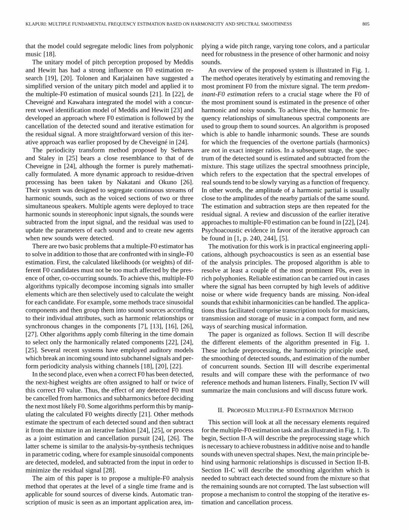
KLAPURI: MULTIPLE FUNDAMENTAL FREQUENCY ESTIMATION BASED ON HARMONICITY AND SPECTRAL SMOOTHNESS 805
that the model could segregate melodic lines from polyphonicmusic [18].
The unitary model of pitch perception proposed by Meddisand Hewitt has had a strong influence on F0 estimation re-search [19], [20]. Tolonen and Karjalainen have suggested asimplified version of the unitary pitch model and applied it tothe multiple-F0 estimation of musical sounds [21]. In [22], deCheveigné and Kawahara integrated the model with a concur-rent vowel identification model of Meddis and Hewitt [23] anddeveloped an approach where F0 estimation is followed by thecancellation of the detected sound and iterative estimation forthe residual signal. A more straightforward version of this iter-ative approach was earlier proposed by de Cheveigné in [24].
The periodicity transform method proposed by Setharesand Staley in [25] bears a close resemblance to that of deCheveigne in [24], although the former is purely mathemati-cally formulated. A more dynamic approach to residue-drivenprocessing has been taken by Nakatani and Okuno [26].Their system was designed to segregate continuous streams ofharmonic sounds, such as the voiced sections of two or threesimultaneous speakers. Multiple agents were deployed to traceharmonic sounds in stereophonic input signals, the sounds weresubtracted from the input signal, and the residual was used toupdate the parameters of each sound and to create new agentswhen new sounds were detected.
There are two basic problems that a multiple-F0 estimator hasto solve in addition to those that are confronted with in single-F0estimation. First, the calculated likelihoods (or weights) of dif-ferent F0 candidates must not be too much affected by the pres-ence of other, co-occurring sounds. To achieve this, multiple-F0algorithms typically decompose incoming signals into smallerelements which are then selectively used to calculate the weightfor each candidate. For example, some methods trace sinusoidalcomponents and then group them into sound sources accordingto their individual attributes, such as harmonic relationships orsynchronous changes in the components [7], [13], [16], [26],[27]. Other algorithms apply comb filtering in the time domainto select only the harmonically related components [22], [24],[25]. Several recent systems have employed auditory modelswhich break an incoming sound into subchannel signals and per-form periodicity analysis withing channels [18], [20], [22].
In the second place, even when a correct F0 has been detected,the next-highest weights are often assigned to half or twice ofthis correct F0 value. Thus, the effect of any detected F0 mustbe cancelled from harmonics and subharmonics before decidingthe next most likely F0. Some algorithms perform this by manip-ulating the calculated F0 weights directly [21]. Other methodsestimate the spectrum of each detected sound and then subtractit from the mixture in an iterative fashion [24], [25], or processas a joint estimation and cancellation pursuit [24], [26]. Thelatter scheme is similar to the analysis-by-synthesis techniquesin parametric coding, where for example sinusoidal componentsare detected, modeled, and subtracted from the input in order tominimize the residual signal [28].
The aim of this paper is to propose a multiple-F0 analysismethod that operates at the level of a single time frame and isapplicable for sound sources of diverse kinds. Automatic tran-scription of music is seen as an important application area, im-
plying a wide pitch range, varying tone colors, and a particularneed for robustness in the presence of other harmonic and noisysounds.
An overview of the proposed system is illustrated in Fig. 1.The method operates iteratively by estimating and removing themost prominent F0 from the mixture signal. The termpredom-inant-F0 estimationrefers to a crucial stage where the F0 ofthe most prominent sound is estimated in the presence of otherharmonic and noisy sounds. To achieve this, the harmonic fre-quency relationships of simultaneous spectral components areused to group them to sound sources. An algorithm is proposedwhich is able to handle inharmonic sounds. These are soundsfor which the frequencies of the overtone partials (harmonics)are not in exact integer ratios. In a subsequent stage, the spec-trum of the detected sound is estimated and subtracted from themixture. This stage utilizes the spectral smoothness principle,which refers to the expectation that the spectral envelopes ofreal sounds tend to be slowly varying as a function of frequency.In other words, the amplitude of a harmonic partial is usuallyclose to the amplitudes of the nearby partials of the same sound.The estimation and subtraction steps are then repeated for theresidual signal. A review and discussion of the earlier iterativeapproaches to multiple-F0 estimation can be found in [22], [24].Psychoacoustic evidence in favor of the iterative approach canbe found in [1, p. 240, 244], [5].
The motivation for this work is in practical engineering appli-cations, although psychoacoustics is seen as an essential baseof the analysis principles. The proposed algorithm is able toresolve at least a couple of the most prominent F0s, even inrich polyphonies. Reliable estimation can be carried out in caseswhere the signal has been corrupted by high levels of additivenoise or where wide frequency bands are missing. Non-idealsounds that exhibit inharmonicities can be handled. The applica-tions thus facilitated comprise transcription tools for musicians,transmission and storage of music in a compact form, and newways of searching musical information.
The paper is organized as follows. Section II will describethe different elements of the algorithm presented in Fig. 1.These include preprocessing, the harmonicity principle used,the smoothing of detected sounds, and estimation of the numberof concurrent sounds. Section III will describe experimentalresults and will compare these with the performance of tworeference methods and human listeners. Finally, Section IV willsummarize the main conclusions and will discuss future work.
II. PROPOSEDMULTIPLE-F0 ESTIMATION METHOD
This section will look at all the necessary elements requiredfor the multiple-F0 estimation task and as illustrated in Fig. 1. Tobegin, Section II-A will describe the preprocessing stage whichis necessary to achieve robustness in additive noise and to handlesounds with uneven spectral shapes. Next, the main principle be-hind using harmonic relationships is discussed in Section II-B.Section II-C will describe the smoothing algorithm which isneeded to subtract each detected sound from the mixture so thatthe remaining sounds are not corrupted. The last subsection willpropose a mechanism to control the stopping of the iterative es-timation and cancellation process.
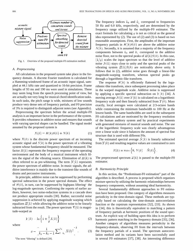
806 IEEE TRANSACTIONS ON SPEECH AND AUDIO PROCESSING, VOL. 11, NO. 6, NOVEMBER 2003
Fig. 1. Overview of the proposed multiple-F0 estimation method.
A. Preprocessing
All calculations in the proposed system take place in the fre-quency domain. A discrete Fourier transform is calculated fora Hamming-windowed frame of an acoustic input signal, sam-pled at 44.1 kHz rate and quantized to 16-bit precision. Framelengths of 93 ms and 190 ms were used in simulations. Thesemay seem long from the speech processing point of view, butare actually not very long for musical chord identification tasks.In such tasks, the pitch range is wide, mixtures of low soundsproduce very dense sets of frequency partials, and F0 precisionof 3% is required to distinguish adjacent notes (see Appendix).
Preprocessing the spectrum before the actual multiple-F0analysis is an important factor in the performance of the system.It provides robustness in additive noise and ensures that soundswith varying spectral shapes can be handled. The signal modelassumed by the proposed system is
(1)
where is the discrete power spectrum of an incomingacoustic signal and is the power spectrum of a vibratingsystem whose fundamental frequency should be measured. Thefactor represents the frequency response of the operatingenvironment and the body of a musical instrument which fil-ters the signal of the vibrating source. Elimination of isoften referred to as pre-whitening. The term representsthe power spectrum of additive noise. In music signals, the ad-ditive interference is mainly due to the transient-like sounds ofdrums and percussive instruments.
In principle, additive noise can be suppressed by performingspectral subtraction in the power spectral domain. The effectof , in turn, can be suppressed by highpass liftering1 thelog-magnitude spectrum. Confirming the reports of earlier au-thors, however, two noise-reduction systems in a cascade doesnot produce appropriate results [30]. Rather, successful noisesuppression is achieved by applying magnitude warping whichequalizes while allowing the additive noise to be linearlysubtracted from the result. The power spectrum is magni-tude-warped as
(2)
where
(3)
1The term “liftering” is defined [29].
The frequency indices and correspond to frequencies50 Hz and 6.0 kHz, respectively, and are determined by thefrequency range utilized by the multiple-F0 estimator. Theexact formula for calculating is not as critical as the generalidea represented by (2). The use of (2) and (3) is based on tworeasonable assumptions. First, the amplitudes of the importantfrequency partials in are above the additive noise
. Secondly, it is assumed that a majority of the frequencycomponents between and correspond to the additivenoise floor, not to the spectral peaks of . In this case,
scales the input spectrum so that the level of additivenoise stays close to unity and the spectral peaks of thevibrating system are noticeably above unity. Itfollows that in (2), additive noise goes through a linear-likemagnitude-warping transform, whereas spectral peaks gothrough a logarithmic-like transform.
The response is efficiently flattened by the loga-rithmic-like transform, since subsequent processing takes placein the warped magnitude scale. Additive noise is suppressedby applying a specific spectral subtraction on [34]. Amoving average over is calculated on a logarithmicfrequency scale and then linearly subtracted from . Moreexactly, local averages were calculated at 2/3-octave bandswhile constraining the minimum bandwidth to 100 Hz at thelowest bands. The same bandwidths are used in the subsequentF0 calculations and are motivated by the frequency resolutionof the human auditory system and by practical experimentswith generated mixtures of musical sounds and noise. The useof the logarithmic frequency scale was clearly advantageousover a linear scale since it balances the amount of spectral finestructure that is used with different F0s.
The estimated spectral average is linearly subtractedfrom and resulting negative values are constrained to zero
(4)
The preprocessed spectrum is passed to the multiple-F0estimator.
B. Harmonicity Principle
In this section, the “Predominant-F0 estimation” part of thealgorithm is described. A process is proposed which organizesmixture spectra by utilizing the harmonic relationships betweenfrequency components, without assuming ideal harmonicity.
Several fundamentally different approaches to F0 estima-tion have been proposed. One category of algorithms measuresperiodicity in the time-domain signal. These methods are typ-ically based on calculating the time-domain autocorrelationfunction or the cepstrum representation [32], [33]. As shownin [34], this is theoretically equivalent to matching a patternof frequency partials atharmonic positionsof the sound spec-trum. An explicit way of building upon this idea is to performharmonic pattern matching in the frequency domain [35], [36].Another category of algorithms measures periodicity in thefrequency-domain, observing F0 from theintervals betweenthe frequency partials of a sound. The spectrum autocorre-lation method and its variants have been successfully usedin several F0 estimators [37], [38]. An interesting difference

KLAPURI: MULTIPLE FUNDAMENTAL FREQUENCY ESTIMATION BASED ON HARMONICITY AND SPECTRAL SMOOTHNESS 807
between the time-domain and frequency-domain periodicityanalysis methods is that the former methods are prone to errorsin F0 halving and the latter to errors in F0 doubling. Thisis because the time-domain signal is periodic at half the F0rate (twice the fundamental time delay) and the spectrum isperiodic at double the F0 rate. A third, psychoacousticallymotivated group of algorithms measures theperiodicity of theamplitude envelopeof a time-domain signal within severalfrequency channels [20], [21], [39].
A major shortcoming of many of the earlier proposedmethods is that they do not handle inharmonic sounds appro-priately. In the case of real nonideal physical vibrators, theharmonic partials are often not in exact integral ratios. Forexample for stretched strings the frequencyof an overtonepartial obeys
(5)
where is the fundamental frequency and is the inhar-monicity factor [40]. Equation (5) means that the partialscannot be assumed to be found at harmonic spectrum positions,but are gradually shifted upwards in the spectrum. This isnot of great concern in speech processing, but is importantwhen analyzing musical sounds at a wide frequency band[41]. In the rest of this paper, capital letteris used to denotefundamental frequency, and the lower case letterto denotesimply frequency.
The proposed predominant-F0 estimation method works bycalculating independent F0 estimates at separate frequencybands and then combining the results to yield a global estimate.This helps to solve several difficulties, one of which is inhar-monicity. According to (5), the higher harmonics may deviatefrom their expected spectral positions, and even the intervalsbetween them are not constant. However, we can assume thespectral intervals to be piecewise constant at narrow-enoughfrequency bands. Thus, we utilize spectral intervals in a twostep process which 1) calculates the weights of differentF0s at separate frequency bands and 2) combines the resultsin a manner that takes inharmonicity into account. Anotheradvantage of bandwise processing is that it provides robustnessand flexibility in the case of badly corrupted signals where onlya fragment of the whole frequency range can be used [41]. Thetwo steps are now described.
1) Bandwise F0 Estimation:The preprocessed spectrumis analyzed at 18 bands that distribute approximately log-
arithmically between 50 Hz and 6 kHz, as illustrated in Fig. 2.Each band comprises a 2/3-octave region of the spectrum,constraining, however, the minimum bandwidth to 100 Hz.Band is subject to weighting with a triangular frequencyresponse , shown in Fig. 2. The overlap between adjacentbands is 50%, making the overall response sum to unity at allexcept the lowest bands. Response at bandis denoted by
(6)
Non-zero frequency components of are defined for fre-quency indices, where is the lowestfrequency component at bandand is the number of com-ponents at the band.
Fig. 2. Magnitude responses of the 18 frequency bands, at which the bandwiseF0 estimation takes place.
In each band, the algorithm calculates a weight vectoracross frequency indices. Note, indexcorresponds to the fun-damental frequency where is the number ofsamples in the time-domain analysis frame andis the sam-pling rate. The resolution of the weight vector is the same asthat of the preprocessed spectrum . The bandwise weights
are calculated by finding a series of each frequencycomponents at bandthat maximizes the sum
(7)
where
(8)
(9)
Here, is the offset of the series of par-tials in the sum, is the number of partials in the sum,and is a normalization factor. A normalization factor isneeded because varies for different values of and . Theform was determined by training with isolated musicalinstrument samples in varying noise conditions. The offsetis varied to find the maximum of (7), which is then stored in
. Different offsets have to be tested because the series ofhigher harmonic partials may have shifted due to inharmonicity.
The upper panel in Fig. 3 illustrates the calculations for asingle harmonic sound at the band between 1100 Hzand 1700 Hz. The arrows indicate the series of frequency com-ponents which maximizes for the true F0.
The values of the offset are restricted to physically realisticinharmonicities, a subset of . The exact limit is not critical,therefore (5) with a constant inharmonicity factor canbe used to determine the maximum allowable offset from theideal harmonic positions. The harmonic indexin (5) can beapproximated by . It follows that the fun-damental partial must be exactly in the harmonic spectralposition, whereas the whole set has to be considered for thehighest partials. In other words, the algorithm combines the useof spectral positions for the lowest harmonic partials and the useof spectral intervals for the higher partials. For a frequency bandwhich is assumed to contain only the first harmonic partial of asound with fundamental frequency corresponding to index,inharmonicity is not allowed. Here is set to 1, and (7) reducesto the special case
(10)

808 IEEE TRANSACTIONS ON SPEECH AND AUDIO PROCESSING, VOL. 11, NO. 6, NOVEMBER 2003
Fig. 3. Calculation of the bandwise F0 weight vectors according to (7).
It follows that in this case the weights are equal tobetween the frequency limits of the band. The algorithm is de-tailed in Table I.
The lower panel in Fig. 3 shows the entire weight vectorcalculated at band for the same signal as in the
upper panel. As can be seen, the preprocessed spectrumappears as such at the corresponding band of . A twicenarrower copy of is found an octave below, since the F0sin that range have exactly one harmonic partial at the band (thesecond partial). Yet lower F0 candidates have a series of higherovertones at the band and inharmonicity is allowed. This is thecase for the true F0 (70 Hz) which has been assigned the highestweight.
An important property of the presented calculations is thatonly the selected frequency samples contribute to the weight
, not the overall spectrum. The other co-occurring soundsaffect the weight only to the extent that their partials overlapthose of the sound being estimated (a solution for overlappingpartials is given in Section II-C). Harmonic selection providesrobustness in sound mixtures as long as we do not rely on thedetection of single partials, as is the case here. Harmonic selec-tion was originally proposed by Parsons in [27] and is used inmost multiple-F0 algorithms, as described in Section I.
2) Integration of Weights Across Subbands:Fig. 4 showsthe calculated weight vectors at different bands for twoisolated piano tones where the weight vectors are arrangedin increasing band center frequency order. As expected, themaximum weight is usually assigned to the true F0, providedthat there is a harmonic partial at that band. The inharmonicityphenomenon appears in Figs. 4(a) and 4(b) as a rising trendin the fundamental frequency.
The bandwise F0 weights are combined to yield a global F0estimate. A straightforward summation across the weight vec-tors does not accumulate them appropriately since the F0 esti-mates at different bands may not match for inharmonic sounds,as can be seen from Fig. 4. To overcome this, the inharmonicityfactor is estimated and taken into account. Two different inhar-monicity models were implemented, the one given in (5) andanother mentioned in [40, p. 363]. In simulations, the perfor-mance difference between the two was negligible. The model in(5) was adopted.
Global weights are obtained by summing squared band-wise weights that are selected from different bands ac-
TABLE IALGORITHM FOR CALCULATING THE WEIGHTSL (n) FORDIFFERENTF0sAT
BAND b. SEE TEXT FOR THEDEFINITION OF SYMBOLS
cording to a curve determined by (5). A search over possiblevalues of is conducted for each, and the highestand the corresponding are stored in the output. Squaringthe bandwise F0 weights prior to summing was found to pro-vide robustness in the presence of strong interference where thepitch may be perceptible only at a limited frequency range.
The global F0 weights and inharmonicity factorsdo not need to be calculated for all fundamental frequency in-dices . Instead, only a set of fundamental frequency indices
is collected from the bandwise weight vec-tors . This is possible, and advantageous since if a soundis perceptible at all, it generally has a high weight in at least oneof the bands. Selecting a couple of maxima from each band pre-serves the correct fundamental frequency among the candidates.
The maximum global weight can be used as such todetermine the true F0. However, an even more robust selec-

KLAPURI: MULTIPLE FUNDAMENTAL FREQUENCY ESTIMATION BASED ON HARMONICITY AND SPECTRAL SMOOTHNESS 809
Fig. 4. Bandwise-calculated F0 weightsL (n) for two piano tones, Figure(a) with F0 65 Hz and Figure (b) with F0 470 Hz. The vectors are displacedvertically for clarity. The true pitches of the tones are indicated with dashedvertical lines.
tion among the candidates can be made by further inspectingthe spectral smoothness of the F0s that have the highest globalweights. This is the reason why a smoothing module is used inFig. 1 before storing the F0. This module will be described indetail in Section III. For the sake of discussion in Section II-Cone can assume that the maximum global score determinesthe predominant F0.
C. Spectral Smoothness Principle
1) Iterative Estimation and Separation:The presentedmethod is capable of making robust predominant-F0 detectionsin polyphonic signals. Moreover, the inharmonicity factor andprecise frequencies of each harmonic partial of the detectedsound are produced. A natural strategy for extending thepresented algorithm to multiple-F0 estimation is to remove thepartials of the detected sound from the mixture and to apply thepredominant-F0 algorithm iteratively to the residual spectrum.
Detected sounds are separated in the frequency domain. Eachsinusoidal partial of a sound is removed from the mixture spec-trum in two stages. First, good estimates of the frequency andamplitude of the partials must be obtained. It is assumed thatthese parameters remain constant in the analysis frame. Second,using the found parameters, the spectrum in the vicinity of the
partials is estimated and linearly subtracted from the mixturespectrum.
Initial estimates for the frequency and amplitude of each si-nusoidal partial of a sound are produced by the predominant-F0detection algorithm. Efficient techniques for estimating moreprecise values have been proposed e.g. in [42]. A methodwidely adopted is to apply Hamming windowing and zeropadding in the time domain, to calculate Fourier spectrum,and to use quadratic interpolation of the spectrum around thepartial. The second problem, estimating the spectrum in thevicinity of the partial is equivalent to translating the magnitudespectrum of the original analysis window at the frequencyof the sinusoidal partial. For Hamming window without zeropadding, it was found to be sufficient to perform the subtractionfor five adjacent frequency bins.
2) The Problem of Coinciding Frequency Partials:Oneissue that is addressed in the algorithm is the problem ofcoinciding frequency partials. To illustrate this problem,simulations were run using the iterative procedure on randomlygenerated F0 mixtures. Fig. 5 shows the errors as a function ofthe musical intervals that occur in the erroneously transcribedsound mixtures (see Appendix). In most cases, the iterativeapproach works rather reliably. However, an important obser-vation can be made when the distribution of the errors in Fig. 5is analyzed. The error rate is strongly correlated with certain F0relations. The conclusion to be noted is that a straightforwardestimation and subtraction approach is likely to fail in caseswhere the fundamental frequencies of simultaneous soundshave simple rational number relations, also calledharmonicrelations. These are indicated over the corresponding bars inFig. 5.
Coinciding frequency partials from different sounds cancause the algorithm to fail since many of the partials coincidein frequency. When the sound detected first is removed, thecoinciding harmonics of remaining sounds are corrupted inthe subtraction procedure. After several iterations, a remainingsound can become too corrupted to be correctly analyzed in theiterations that follow.
When two sinusoidal partials with amplitudesand andphase difference coincide in frequency, the amplitude of theresulting sinusoid can be calculated as
(11)
If the two amplitudes are roughly equivalent, the partials mayeither amplify or cancel each other, depending on. However,if one of the amplitudes is significantly greater than the other,as is usually the case, approaches the maximum of the two.
Assuming ideal harmonicity, it is straightforward to provethat the harmonic partials of two sounds coincide if and onlyif the fundamental frequencies of the two sounds are in rationalnumber relations. Moreover, if the harmonic indices of the co-inciding partials are and , then every partial of the firstsound coincides with every partial of the other sound. Animportant principle in Western music is to pay attention to thepitch relationships of simultaneously played notes. Simple har-monic relationships are favored over dissonant ones in order tomake the sounds blend better. Because harmonic relationships

810 IEEE TRANSACTIONS ON SPEECH AND AUDIO PROCESSING, VOL. 11, NO. 6, NOVEMBER 2003
Fig. 5. Distribution of the F0 estimation errors as a function of the musicalintervals that occur in the erroneously transcribed sound mixtures.
are so common in music, these “worst cases” must be handledwell in general.
To solve this problem, the spectra of the detected sounds mustbe smoothed before subtracting them from the mixture. Con-sider the preprocessed spectrum of a two-sound mixturein Fig. 6(a). In the figure, the harmonic partials of the higher-pitched sound coincide with every third harmonic of the lower-pitched sound . As predicted by (11), thecoinciding partials randomly cancel or amplify each other at thelow frequencies, whereas at the higher frequencies the summaryamplitudes approach the maximum of the two, i.e., the spectralenvelope of the higher sound.
When the spectrum of the lower-pitched sound is smoothed(the thin slowly decreasing horizontal curve in Fig. 6(b)), the co-inciding partials at the higher frequencies rise above the smoothspectrum and thus remain in the residual after subtraction. Inparticular, this solves a very common case where the dense har-monic series of a lower-pitched sound matches the few partialsof a higher-pitched sound. Detecting the higher-pitched soundfirst is less common and in that case, only a minority of the har-monics of the lower-pitched sound are deleted.
It should be noted that simply smoothing the amplitude enve-lope (the thin curve in Fig. 6(b)) of a sound before subtractingit from the mixture does not result in lower error rates. A suc-cessful smoothing algorithm was found by applying psychoa-coustic knowledge. The full motivation for this approach hasbeen presented in [43] and is beyond the scope of this paper.
The algorithm first calculates a moving average over the am-plitudes of the harmonic partials of a sound. An octave-widetriangular weighting window is centered at each harmonic par-tial , and the weighted mean of the amplitudes of the par-tials in the window is calculated. This is the smooth spectrumillustrated by a thin horizontal curve in Fig. 6(b). The originalamplitude value is then replaced with the minimum of theoriginal and :
(12)
These values are illustrated by a thick curve in Fig. 6(b).Performing this straightforward smoothing operation beforesubtracting the sound from the mixture reduces the error ratessignificantly.
A further improvement to the smoothing method can be madeby utilizing the statistical dependency of every harmonic
Fig. 6. Illustration of the spectral smoothness principle. (a) PreprocessedspectrumZ(k) containing two sounds with F0s in the relation 1:3. (b) Twodifferent smoothing operations have been used to estimate the spectral envelopeof the lower-pitched sound. The results are indicated with thin and thickhorizontal curves.
partial, as was previously explained following (11) in this sec-tion. The algorithm applies a multistage filter with the followingsteps [43]. First, the indices of theharmonic partials around harmonicare collected from an oc-tave-wide window. Next, the surrounding partials are classifiedinto groups, where all the harmonics that share a common di-visor are put in the same group, starting from the smallest primefactors. Third, weighted mean around harmonicis calculatedinside groups in the manner described above. In the last step,the estimates of different groups are averaged, weighting eachgroup according to its mean distance from harmonic.
3) Recalculation of F0 Weights After Smoothing:The de-scribed principle of smoothing provides an efficient solutionto another common class of errors. In this class of errors twoor more fundamental frequencies in specific relationships maycause the detection of a nonexistent sound, such as the root of amusical chord in its absence. For instance, when two harmonicsounds with fundamental frequencies and are played,the spectra of these sounds match every second and every thirdharmonic partial of a nonexisting sound with fundamental fre-quency . This frequency may be erroneously estimated inthe predominant-F0 calculations given the observed partials.
The problem can be solved by applying smoothing and anordered search when selecting among the candidate indicescalculated by the predominant-F0 algorithm (see the end of Sec-tion II-B). First, the candidate with the highest global weight
is taken and its spectrum is smoothed. Then the weightof this candidate is recalculated using the smoothed harmonicamplitudes. In the above-described case of a nonexistent sound,the irregularity of the spectrum decreases the level of the smoothspectrum significantly, and the weight remains low. If the recal-culated weight drops below the second-highest weight, the next

KLAPURI: MULTIPLE FUNDAMENTAL FREQUENCY ESTIMATION BASED ON HARMONICITY AND SPECTRAL SMOOTHNESS 811
candidate is processed, and this is continued. The highest re-calculated global weight determines the F0. The computationalload of applying smoothing and recalculation to select amongthe candidates is negligible, since the recalculation procedurehas to consider only one F0 and one value ofin (7).
D. Estimating the Number of Concurrent Sounds
A mechanism is needed which controls the stopping of theiterative F0 estimation and sound separation process. This leadsto the estimation of the number of concurrent sounds, i.e. thepolyphony. The difficulty of the task is comparable to that offinding the F0 values themselves. Huron has studied musicians’ability to identify the number of concurrently sounding voicesin polyphonic textures [44]. According to his report by four-voice polyphonies the test subjects underestimated the numberof voices in more than half of the cases.
A statistical-experimental approach was taken to solve theproblem. Random mixtures of one to six concurrent harmonicsounds were generated by allotting sounds from McGill Uni-versity Master Samples collection [45]. The mixtures were thencontaminated with pink noise or random drum sounds fromRoland R-8 mk II drum machine. Signal-to-noise ratio wasvaried between 23 dB and2 dB.
The behavior of the iterative multiple-F0 estimation systemwas investigated using these artificial mixtures with knownpolyphonies. Based on this investigation it was decided tosplit the estimation task into two stages. The first stage detectsif there are any harmonic sounds at all in the input, and thesecond estimates the number of concurrent sounds, if the firsttest has indicated that some are present. It was found that thebest single feature to indicate the presence of harmonic soundswas the global weight of the winning F0 candidate atthe first iteration. The best compound feature consists ofand terms related to the signal-to-noise ratio (SNR) of the inputsignal:
(13)Here is the discrete power spectrum of the input signaland is the power spectrum of the estimated noise,obtained by applying inverse transform of (2) on . Fre-quency indices and are the same as in (3). A signal isdetermined to contain harmonic sounds whenis greater thana fixed threshold.
If an analysis frame has been determined to contain harmonicsounds, another model is used to estimate the number of sounds.The maximum global weight at iteration was again thebest single feature for controlling the iteration stopping. How-ever, the weight values are affected by the SNR gettingsmaller in noise. The bias can be explicitly corrected, resultingin the measure
(14)
As long as the value of stays above a fixed threshold, thesound detected at iterationis accepted as a valid F0 estimateand the iteration is continued. In (13) and (14), the SNR-relatedterms have different roles and thus different signs.
III. RESULTS
A. Experimental Setup
Simulations were run to validate the proposed methods. Theacoustic database consisted of samples from four differentsources. The McGill University Master Samples collection [45]and independent recordings for acoustic guitar were availablealready during the development phase of the system. In orderto verify that the results generalize outside these data sets, thesamples from the University of Iowa website [46] and IRCAMStudio Online [47] were added to the final evaluation set. Therewere altogether 30 different musical instruments, comprisingbrass and reed instruments, strings, flutes, the piano, and theguitar. These introduce several different sound productionmechanisms and a variety of spectra. On the average, therewere 1.8 pieces of each of the 30 instruments and 2.5 differentplaying styles per instrument. The total number of sampleswas 2536. These were randomly mixed to generate test cases.The instruments marimba and the vibraphone were excludedfrom the data set since their spectrum is quite different fromthe others and extremely inharmonic. The system admittedlycannot handle these sounds reliably.
Semirandom sound mixtures were generated according totwo different schemes.Random mixtureswere generated byfirst allotting an instrument and then a random note from itswhole playing range, restricting, however, the pitch over fiveoctaves between 65 Hz and 2100 Hz. The desired number ofsimultaneous sounds were allotted and then mixed with equalmean-square levels.Musical mixtureswere generated in a sim-ilar manner, but favoring different pitch relationships accordingto a statistical profile discovered by Krumhansl in classicalWestern music [48, p. 68]. In brief, octave relationships arethe most frequent, followed by consonant musical intervals,and the smallest probability of occurrence is given to dissonantintervals. In general, musical mixtures are more difficult toresolve (see Section II-C2).
Acoustic input was fed to the multiple-F0 algorithm that es-timated F0s in a single time frame. Unless otherwise stated, thenumber of F0s to extract, i.e., the polyphony, was given alongwith the mixture signal. It was found to be more informative tofirst evaluate the multiple-F0 estimator without the polyphonyestimator, because these two are separable tasks and because thereference methods do not implement polyphony estimation. Theconfiguration and parameters of the system were fixed unlessotherwise stated. A correct F0 estimate was defined to deviateless than half a semitone (3%) from the true value, makingit “round” to a correct note on a Western musical scale. Errorssmaller than this are not significant from the point of view ofmusic transcription.
B. Reference Methods
To put the results in perspective, two reference methods wereused as a baseline in simulations. The first method,YIN, is a

812 IEEE TRANSACTIONS ON SPEECH AND AUDIO PROCESSING, VOL. 11, NO. 6, NOVEMBER 2003
state-of-the-artmonophonicF0 estimator for speech and musicsignals [49]. Naturally, the method can be used as a baseline insingle-F0 analysis only. The algorithm has been designed to bereliable for individual analysis frames and has been thoroughlytested and compared with other methods in [49]. The originalimplementation by the authors was employed and parameterswere left intact except the “absolute threshold” which was fine-tuned to value 0.15 to improve the performance.
The other reference method, referred to asTK, is a mul-tiple-F0 estimator proposed by Tolonen and Karjalainen in[21]. The implementation was carefully prepared based on thereference, and the original code by the authors was used inthe warped linear prediction part of the algorithm. Thoroughtesting was carried out to verify the implementation. Originalparameters given in [21] were applied. As reported by theauthors, the method cannot handle “spectral pitch,” i.e., F0sabove 1 kHz. It was further found out here that the method isbest at detecting F0s in the three-octave range between 65 Hzand 520 Hz. Thus, in the simulations that follow, the mixturesgiven to theTK method were restricted to contain F0s beloweither 520 Hz or 1 kHz. The bound is specified for each case inthe simulation results to follow.
C. Experimental Results
In the first experiment, different F0 estimators are compared.For this experiment, a predominant-F0 estimate (firstly detectedF0) was defined to be correct if it matches the correct F0 ofanyof the component sounds. That is, only a single match among allpossible F0s is required in this error measure. The error rate wascalculated as the amount of predominant-F0 errors divided bythe number of random sound mixtures (1000), not by the numberof reference notes (e.g. 6000 in the six-note mixtures). F0 esti-mation was performed in a single 190 ms time frame 100 msafter the onset of the sounds. Fig. 7 shows the error rates for thepredominant-F0 estimation in different polyphonies. Results aregiven for the proposed system and for the two reference systems.
For the proposed system, the error rates are generally below10%, getting close only in six-note polyphonies. Surprisingly,increasing the number of concurrent sounds from one to twoappears to help lower the error rate of detecting at least one F0correctly. However, this is due to the fact that the acoustic data-base contains a small percentage of irregular sounds for whichthe simple model in (7) does not work. Among these are e.g.high flute tones and high plucked string tones. Two-sound mix-tures are more likely to contain at least one clear sound with noanomalities, which then appears as the predominant F0.
TheYIN method achieves 4.1% error rate for isolated notes.Since the method is not intended for multiple-F0 estimation, it isnot fair to make comparison for polyphonic signals. Like othersingle-F0 estimators, the algorithm converges to 70% error ratealready in three-note mixtures. TheTKmethod is not quite as re-liable for single-pitch signals, but works robustly in polyphony.If the method is given F0s only below 520 Hz, the predomi-nant-F0 detection accuracy comes close to the proposed systemin higher polyphonies. This is partly due to the relatively higherrandom guess rate.
In the second experiment, the performance of multiple-F0 es-timation is explored in more detail. For multiple-F0 estimation,
Fig. 7. Error rates for detecting any of the potential F0s in a sound as a functionof the predominant-F0 estimation algorithm and the polyphony.
a more appropriate error measure is anote error rate (NER)metric. The NER is defined as the sum of the F0s in error di-vided by the number of F0s in the reference transcription. Theerrors are of three types:
a) Substitution errors. These are defined as errors in which agiven F0 is detected but the estimated value differs morethan 3% from the reference.
b) Deletion errors have occurred if the number of detectedF0s is smaller than the number of F0s in the reference.
c) Insertion errors have occurred if the number of detectedF0s exceeds that in the reference.
Substitution and deletion errors together can be counted fromthe number of F0s in the reference that are not correctly es-timated. Insertion errors can be counted from the number ofexcessive estimates.
Results for multiple-F0 estimation in different polyphoniesare shown in Fig. 8. Here the number of concurrent sounds toextract was given for each mixture signal, i.e., the polyphonywas known. Thus insertion and deletion errors do not occur.Random and musical sound mixtures were generated accordingto the described schemes, and the estimator was then requestedto find a given number of F0s in a single 190 ms time frame 100ms after the onset of the sounds.
In Fig. 8, the bars represent the overall NER’s as a function ofthe polyphony. As can be seen, the NER for random four-soundpolyphonies is 9.9% on the average. The different shades ofgray in each bar indicate the error cumulation in the iteration,errors which occurred in the first iteration at the bottom, anderrors of the last iteration at the top. As a general impression,the system works reliably and exhibits graceful degradation inincreasing polyphony. Results for musical mixtures are slightlyworse than for random mixtures (see Section II-C2), but thedifference is not great. This indicates that the spectral smoothingprinciple works well in resolving harmonically related pitchcombinations.
Analysis of the error cumulation reveals that the errors whichoccurred in the last iteration account for approximately half ofthe errors in all polyphonies, and the probability of error in-creases rapidly in the course of iteration. Besides indicating thatthe subtraction process does not work perfectly, the conductedlistening tests suggest that this is a feature of the problem it-self, rather than only a symptom of the algorithms used. In mostmixtures, there is a sound or two that are very difficult to per-ceive because their spectrum is virtually hidden under the othersounds.
For the reference methodTK, note error rates for mixturesranging from one to six sounds were 22%, 31%, 39%, 45%,

KLAPURI: MULTIPLE FUNDAMENTAL FREQUENCY ESTIMATION BASED ON HARMONICITY AND SPECTRAL SMOOTHNESS 813
Fig. 8. Note error rates for multiple-F0 estimation using the proposedalgorithm when the polyphony was known. Bars represent the overall errorrates, and the different shades of gray the error cumulation in iteration.
49%, and 53%, respectively, when F0s were resticted to range65 Hz–1 kHz. For the three-octave range between 65 Hz and 520Hz, the corresponding error rates were 7.5%, 17%, 26%, 34%,38%, and 43%. Given the complexity of the problem, even theseerror rates are rather low.
Table II gives the error rates for different system configura-tions. Different processing elements were disabled one-by-onein order to evaluate their importance. In each case, the systemwas kept otherwise fixed. In the first test, the mechanisms thataccommodate inharmonicity were disabled. One mechanism isin bandwise F0-weight calculations, and in this case the offset
in (7) was constrained to a value which corresponds to anideal harmonicity. Another mechanism is in the integrationphase. Here the inharmonicity factor was constrained to zero,leading to a straightforward summing across squared weightvectors. The resulting performance degradation is mostly dueto the bandwise calculations.
In the second test, the spectral smoothing algorithm wasswitched between the one presented in Section II-C2 anda version which leaves the harmonic series intact. Thesmoothing operation made a significant improvement to mul-tiple-F0 estimation accuracy in all polyphonies, except for thesingle-note case where it did not have a noticeable effect on theperformance.
In all the results presented above, the polyphony of the sig-nals was known. Fig. 9 shows the statistical error rate of theoverall multiple-F0 estimation system when the polyphony isestimated in the analysis frame, as described in Section II-D. Re-sults are shown for two different polyphony estimation thresh-olds (i.e., thresholds for in (14) which were 0.65 and 1.1 forthe left and right panels, respectively). Depending on the appli-cation, either overestimating or underestimating the number ofconcurrent sounds may be more harmful. In a music transcrip-tion system, for example, extraneous notes in the output are verydisturbing. However, if the frame-level F0 estimates are furtherprocessed at a higher level, it is usually advantageous to producetoo many rather than too few note candidates.
In general, the proposed polyphony estimation methodoperates robustly. However, when the estimation threshold istuned to avoid extraneous detections in monophonic signals,the polyphony is underestimated in higher polyphonies. On theother hand, when underestimations are avoided, many of the
TABLE IIERROR RATES FORDIFFERENT SYSTEM CONFIGURATIONS WHEN THE
POLYPHONY OF THESIGNALS WAS KNOWN
Fig. 9. Error rates for the two different polyphony estimations strategies.
extraneous F0s appear in monophonic signals. This is likelyto be characteristic of the problem itself (see Huron’s report[44] mentioned in Section II-D). One or two sounds in richpolyphonies are usually very difficult to distinguish.
Table III shows the influence of shortening the analysis frame.The significant difference between 190 ms and 93 ms framesizes is partly caused by the fact that the applied techniquewas sometimes not able to resolve the F0 with the required
3% accuracy. Also, irregularities in the sounds themselves,such as vibrato, are more difficult to handle in short frames.However, when the time frame was shortened from 190 msto 93 ms, the error rate of the reference methodTK increasedonly by approximately 5% for both 1000 Hz and 520 HzF0 limits and in all polyphonies. Thus, the error rates ofTKwere essentially the same as those presented around Fig. 8.While the performance is still clearly worse than that of theproposed method (polyphony was known), an obvious drawbackof the proposed method is that its accuracy depends on thelength of the analysis frame. A basic reason for this is thatthe linear frequency resolution of spectral methods does notsuffice at the low end, whereas the frequency resolution ofautocorrelation-based methods is proportional to the inverse offrequency, being closer to the logarithmic frequency resolutionof musical scales and human hearing. Despite these differences,reliable multiple-F0 estimation in general seems to requirelonger time frames than single-F0 estimation.
Fig. 10 shows the NER’s in different types and levels ofadditive noise when the polyphony was known. Pink noise wasgenerated in the band between 50 Hz and 10 kHz. Percussioninstrument interference was generated by randomizing drumsamples from a Roland R-8 mk II drum machine. The test setcomprised 33 bass drum, 41 snare, 17 hi-hat, and 10 cymbal

814 IEEE TRANSACTIONS ON SPEECH AND AUDIO PROCESSING, VOL. 11, NO. 6, NOVEMBER 2003
TABLE IIIERRORRATES FORDIFFERENTANALYSIS FRAME LENGTHS
Fig. 10. Error rates in additive pink noise (left panel) and with interferingpercussive sounds (right panel). For both noise types, error rates for a cleansignal and for noisy signals with SNR’s 10 dB, 5 dB, and 0 dB are given.Polyphony was known.
sounds. The signal-to-noise ratio was adjusted within the anal-ysis frame, and the ratio was defined between the noise and thesumof the harmonic sounds. Thus, the SNR from the point ofview of individual sounds is much worse in higher polyphonies.A 190 ms frame was applied.
D. Comparison With Human Performance
Listening tests were conducted to measure the human pitchidentification ability, particularly the ability of trained musi-cians to transcribe polyphonic sound mixtures. Detailed anal-ysis of the results is beyond the scope of this article. Only asummary of the main findings can be reviewed here.
Test stimuli consisted of computer-generated mixtures of si-multaneously onsetting sounds that were reproduced using sam-pled Steinway grand piano sounds from the McGill UniversityMaster Samples collection [45]. The number of co-occurringsounds varied from two to five. The interval between the highestand the lowest pitch in each individual mixture was never widerthan 16 semitones in order to make the task feasible for the sub-jects that did not have “absolute pitch”, i.e., the rare ability ofbeing able to name the pitch of a sound without a referencetone. Mixtures were generated from three pitch ranges (i.e., reg-isters): low (33 Hz–130 Hz), middle (130 Hz–520 Hz), and high(520 Hz–2100 Hz). In total, the test comprised 200 stimuli.
The task was to write down the musical intervals, i.e., pitch re-lations, of the presented sound mixtures. Absolute pitch valueswere not asked for and the number of sounds in each mixturewas given. Thus, the test resembles the musical interval andchord identification tests that are a part of the basic musicaltraining in Western countries.
Fig. 11. Chord error rates of the human listeners (curves) and of the proposedalgorithm (bars) for different stimulus categories. The lowest curve representsthe two most skilled subjects, the middle curve the average of all subjects, andthe highest curve the two clearly weakest subjects. The labels of the simuluscategories consist of a number which signifies the polyphony, and of a letterwhich tells the pitch range used.
A total of ten subjects participated in the test. All of them weretrained musicians in the sense of having taken several years ofear training2 in music. Seven subjects were students of musi-cology at university level. Two were more advanced musicians,possessing absolute pitch and exceptional pitch identificationabilities. One subject was an amateur musician of similar mu-sical ability as the seven students.
Fig. 11 shows the results of the listening test. Chord error rates(CER) are plotted for different stimulus categories. CER is thepercentage of sound mixtures where one or more pitch identi-fication errors occurred. The labels of the categories consist ofa number which signifies the polyphony, and of a letter whichtells the pitch range used. Letter “m” refers to the middle, “h” tothe high, and “l” to the low register. Performance curves are av-eraged over three different groups. The lowest curve representsthe two most skilled subjects, the middle curve the average of allsubjects, and the highest curve the two clearly weakest subjects.
The CER’s cannot be directly compared to the NER’s givenin Fig. 8. The CER metric is more demanding, accepting onlysound mixtures where all pitches are correctly identified. It hadto be adopted to unambiguously process the musicians’ answers,which were given as pitch intervals.
For the sake of comparison, the stimuli and performancecriteria used in the listening test were used to evaluate theproposed computational model. Five hundred instances weregenerated from each category included in Fig. 11, using thesame software that randomized samples for the listening test.These were fed to the described multiple-F0 system. The CERmetric was used as a performance measure.
The results are illustrated with bars in Fig. 11. As a generalimpression, only the two most skilled subjects perform betterthan the computational model. However, performance differ-ences in high and low registers are quite revealing. The devisedalgorithm is able to resolve combinations of low sounds thatare beyond the ability of human listeners. This seems to be dueto the good frequency resolution applied. On the other hand,
2The aim of ear training in music is to develop the faculty of discriminatingsounds, recognizing musical intervals, and playing music by ear, i.e., withoutthe aid of written music.

KLAPURI: MULTIPLE FUNDAMENTAL FREQUENCY ESTIMATION BASED ON HARMONICITY AND SPECTRAL SMOOTHNESS 815
human listeners perform relatively well in the high register. Thisis likely to be due to an efficient use of the temporal features,onset asynchrony and different decay rates, of high piano tones.These were not available in the single time frame given to themultiple-F0 algorithm.
IV. CONCLUSIONS
The paper shows that multiple-F0 estimation can be per-formed reasonably well using only spectral cues, harmonicityand spectral smoothness, without the need for additionallong-term temporal features. For a variety of musical sounds,a prior knowledge of the type of sound sources involved isnot necessary, although adaptation of internal source (e.g.instrument) models would presumably further enhance theperformance.
The primary problem in multiple-F0 estimation appears tobe in associating partials correctly with their individual sourcesof production. The harmonicity principle must be applied ina manner that is flexible enough to accommodate a realisticamount of inharmonicity in sound production, and yet con-straining enough to prevent erroneous groupings. Contrastedwith the complexity needed in handling inharmonicity, theharmonic summation model used to calculating F0 weightsfrom the amplitudes of the grouped partials is very simple, asembodied in (8) and (9).
A spectral smoothing approach was proposed as an effi-cient new mechanism in multiple-F0 estimation and spectralorganization. The introduction of this principle corrected ap-proximately half of the errors occurring in a system which wasotherwise identical but did not use the smoothness principle.
An attractive property of the iterative estimation and separa-tion approach is that at least a couple of the most prominent F0scan be detected even in very rich polyphonies. The probabilityof error increases rapidly in the course of the iteration, but on thebasis of the listening tests it was suggested that this is at least inpart due to the inherent characteristics of the problem itself. Thelast iteration, i.e., estimation of the F0 of the sound detected last,accounts for approximately half of the errors in all polyphonies.
The main drawback of the presented method is that it re-quires a relatively long analysis frame in order to operate re-liably for low-pitched sounds. This is largely due to the fact thatthe processing takes place in the frequency domain where suffi-ciently fine frequency resolution is required for harmonic seriesof low-pitched sounds.
The described method has been applied to the automatic tran-scription of continuous music on CD recordings. Some demon-stration signals are provided at [50]. Contrary to the musicalchord identification task, however, the accuracy is not compa-rable to that of trained musicians. There are several possibilitiesthat can be explored as areas of future development. Integra-tion across multiple time frames can be used to improve perfor-mance. While independent multiple-F0 estimation in each timeframe is important for feature extraction, it does not account forthe real experience represented in a human listener. Analogousto the case of speech recognition in which models of words andlanguage are used to improve performance, use of higher-levelfeatures in music are also expected to improve music estimationand transcription tasks.
TABLE IVSOME BASIC MUSICAL INTERVALS
APPENDIX
Western music typically uses awell-temperedmusical scale.That is, the notes are arranged on a logarithmic scale where thefundamental frequency of a note is .
The notes on a standard piano keyboard range fromup to . The termsemitonerefers to the interval betweentwo adjacent notes and is used to measure other musical inter-vals. The F0 relation of two notes that are one semitone apart is
.Although the well-tempered scale is logarithmic, it can
surprisingly accurately generate F0s that are in rational numberrelations. Table IV lists some basic musical intervals and thecorresponding ideal rational number relations. Intervals whichapproximate simple rational number relationships are calledharmonic, or, consonantintervals, as opposed todissonantintervals.
REFERENCES
[1] S. Bregman,Auditory Scene Analysis: The Perceptual Organization ofSound. Cambridge, MA: MIT Press, 1990.
[2] L. R. Rabiner, M. J. Cheng, A. E. Rosenberg, and C. A. McGonegal, “Acomparative performance study of several pitch detection algorithms,”IEEE Trans. Acoust., Speech, Signal Processing, vol. ASSP-24, no. 5,pp. 399–418, 1976.
[3] W. J. Hess, “Pitch and voicing determination,”Advances in SpeechSignal Processing, 1991.
[4] A. de Cheveigné and H. Kawahara, “Comparative evaluation of F0 esti-mation algorithms,” inProc. Eurospeech, Copenhagen, Denmark, 2001,pp. 2451–2454.
[5] W. M. Hartmann, “Pitch, periodicity, and auditory organization,”J.Acoust. Soc. Amer., vol. 100, no. 6, pp. 3491–3502, 1996.
[6] J. A. Moorer, “On the transcription of musical sound by computer,”Comput. Music J., pp. 32–38, Nov. 1977.
[7] C. Chafe and D. Jaffe, “Source separation and note identification in poly-phonic music,” inProc. IEEE Int. Conf. Acoust., Speech, Signal Pro-cessing, Tokyo, 1986, pp. 1289–1292.
[8] R. C. Maher, “Evaluation of a method for separating digitized duet sig-nals,”J. Audio Eng. Soc., vol. 38, no. 12, pp. 956–979, 1990.
[9] H. Katayose and S. Inokuchi, “The Kansei music system,”Comput.Music J., vol. 13, no. 4, pp. 72–77, 1989.
[10] M. Hawley, “Structure Out of Sound,” Ph.D. dissertation, MIT MediaLaboratory, Cambridge, MA, 1993.
[11] L. Rossi, “Identification de sons polyphoniques de piano,” Ph.D. thesis,L’Universite de Corse, Corsica, France, 1998.
[12] D. F. Rosenthal and H. G. Okuno, Eds.,Computational Auditory SceneAnalysis. Mahwah, NJ: Lawrence Erlbaum, 1998.
[13] K. Kashino, K. Nakadai, T. Kinoshita, and H. Tanaka, “Organization ofhierarchical perceptual sounds: music scene analysis with autonomousprocessing modules and a quantitative information integration mecha-nism,” in Proc. Int. Joint Conf. Artificial Intelligence, Montréal, QC,Canada, 1995.

816 IEEE TRANSACTIONS ON SPEECH AND AUDIO PROCESSING, VOL. 11, NO. 6, NOVEMBER 2003
[14] K. D. Martin, “Automatic Transcription of Simple Polyphonic Music:Robust Front End Processing,” Massachusetts Institute of TechnologyMedia Laboratory Perceptual Computing Section, Tech. Rep. 399, 1996.
[15] D. P. W. Ellis, “Prediction-Driven Computational Auditory Scene Anal-ysis,” Ph.D. thesis, MIT Media Laboratory, Cambridge, Massachusetts,1996.
[16] M. Goto, “A robust predominant-F0 estimation method for real-time de-tection of melody and bass lines in CD recordings,” inProc. IEEE In-ternational Conf. on Acoust., Speech, and Signal Processing, Istanbul,Turkey, June 2000.
[17] G. J. Brown and M. P. Cooke, “Perceptual grouping of musical sounds:a computational model,”J. New Music Res., vol. 23, pp. 107–132, 1994.
[18] D. Godsmark and G. J. Brown, “A blackboard architecture for computa-tional auditory scene analysis,”Speech Commun., vol. 27, pp. 351–366,1999.
[19] R. Meddis and M. J. Hewitt, “Virtual pitch and phase sensitivity of acomputer model of the auditory periphery I: pitch identification,”J.Acoust. Soc. Amer., vol. 89, no. 6, pp. 2866–2882, 1991.
[20] R. Meddis and L. O’Mard, “A unitary model of pitch perception,”J.Acoust. Soc. Amer., vol. 102, no. 3, pp. 1811–1820, 1997.
[21] T. Tolonen and M. Karjalainen, “A computationally efficient multip-itch analysis model,”IEEE Trans. Speech Audio Processing, vol. 8, pp.708–716, Nov. 2000.
[22] A. de Cheveigné and H. Kawahara, “Multiple period estimation andpitch perception model,”Speech Commun., vol. 27, pp. 175–185, 1999.
[23] R. Meddis and M. J. Hewitt, “Modeling the identification of concurrentvowels with different fundamental frequencies,”J. Acoust. Soc. Amer.,vol. 91, no. 1, pp. 233–245, 1992.
[24] A. de Cheveigné, “Separation of concurrent harmonic sounds: funda-mental frequency estimation and a time-domain cancellation modelof auditory processing,”J. Acoust. Soc. Amer., vol. 93, no. 6, pp.3271–3290, 1993.
[25] W. A. Sethares and T. W. Staley, “Periodicity transforms,”IEEE Trans.Signal Processing, vol. 47, no. 11, pp. 2953–2964, 1999.
[26] T. Nakatani and H. G. Okuno, “Harmonic sound stream segregationusing localization and its application to speech stream segregation,”Speech Commun., vol. 27, pp. 209–222, 1999.
[27] T. W. Parsons, “Separation of speech from interfering speech by meansof harmonic selection,”J. Acoust. Soc. Amer., vol. 60, pp. 911–918,1976.
[28] T. Verma, “A Perceptually Based Audio Signal Model With Applicationto Scalable Audio Compression,” Ph.D. dissertation, Stanford Univer-sity, 2000.
[29] L. R. Rabiner and B.-H. Juang,Fundamentals of Speech Recogni-tion. Englewood Cliffs, NJ: Prentice-Hall, 1993.
[30] H. Hermansky, N. Morgan, and H.-G. Hirsch, “Recognition of speech inadditive and convolutive noise based on RASTA spectral processing,”in Proc. IEEE Int. Conf. Acoustics, Speech, Signal Processing, Min-neapolis, Minnesota, 1993.
[31] A. P. Klapuri, “Automatic transcription of musical recordings,” inProc.Consistent and Reliable Acoustic Cues Workshop, Aalborg, Denmark,Sep. 2001.
[32] D. Talkin, “A robust algorithm for ptch tracking,” inSpeech Coding andSynthesis, W. B. Kleijn and K. K. Paliwal, Eds: Elseview Science B.V.,1995.
[33] J. C. Brown and B. Zhang, “Musical frequency tracking using themethods of conventional and “narrowed” autocorrelation,”J. Acoust.Soc. Amer., vol. 89, no. 5, pp. 2346–2354, 1991.
[34] A. P. Klapuri, “Qualitative and quantitative aspects in the design of pe-riodicity estimation algorithms,” inProc. European Signal ProcessingConference, Tampere, Finland, Sept. 2000.
[35] B. Doval and X. Rodet, “Estimation of fundamental frequency of mu-sical sound signals,” inProc. IEEE Int. Conf. on Acoust., Speech, andSignal Processing, 1991, pp. 3657–3660.
[36] J. C. Brown, “Musical fundamental frequency tracking using a pat-tern recognition method,”J. Acoust. Soc. Amer., vol. 92, no. 3, pp.1394–1402, 1992.
[37] M. Lahat, R. J. Niederjohn, and D. A. Krubsack, “A spectral autocorrela-tion method for measurement of the fundamental frequency of noise-cor-rupted speech,”IEEE Trans. Acoust., Speech, Signal Processing, vol.ASSP-35, no. 6, pp. 741–750, 1987.
[38] N. Kunieda, T. Shimamura, and J. Suzuki, “Robust method of mea-surement of fundamental frequency by ACLOS—autocorrelation of logspectrum,” inProc. IEEE Int. Conf. on Acoust., Speech, and Signal Pro-cessing, 1996, pp. 232–235.
[39] A. J. M. Houtsma, “Pitch perception,” inHearing—Handbook of Per-ception and Cognition, B. J. C. Moore, Ed. San Diego, CA: Academic,1995.
[40] N. F. Fletcher and T. D. Rossing,The Physics of Musical Instruments,2nd ed. New York: Springer-Verlag, 1998.
[41] A. P. Klapuri, “Wide-band pitch estimation for natural sound sourceswith in harmonicities,” inProc. 106th Audio Eng. Soc. Convention, Mu-nich, Germany, 1999.
[42] X. Rodet, “Musical sound signal analysis/synthesis: sinusoidal+
residual and elementary waveform models,” inProc. IEEE Time-Fre-quency and Time-Scale Workshop, Coventry, U.K., Aug. 1997.
[43] A. P. Klapuri, “Multipitch estimation and sound separation by the spec-tral smoothness principle,” inProc. IEEE Int. Conf. on Acoust., Speech,and Signal Processing, 2001, pp. 3381–3384.
[44] D. Huron, “Voice denumerability in polyphonic music of homogeneoustimbres,”Music Perception, vol. 6, no. 4, pp. 361–382, Summer 1989.
[45] F. Opolko and J. Wapnick,McGill University Master Samples. Montreal, QC, Canada: McGill University, 1987.
[46] The University of Iowa Musical Instrument Sam-pleshttp://theremin.music.uiowa.edu/[Online]
[47] IRCAM Studio Onlinehttp://soleil.ircam.fr/[Online][48] C. L. Krumhansl,Cognitive Foundations of Musical Pitch. New York:
Oxford Univ. Press, 1990.[49] A. de Cheveigné and H. Kawahara, “YIN, a fundamental frequency es-
timator for speech and music,”J. Acoust. Soc. Amer., vol. 111, no. 4,April 2002.
[50] Automatic Transcription of Music Demonstrations, A. P. Kla-puri.http://www.cs.tut.fil/~klap/iiro/[Online]
Anssi P. Klapuri was born in Kälviä, Finland, in 1973. He received the M.Sc.degree in information technology from the Tampere University of Technology(TUT), Tampere, Finland, in June 1998. He is currently pursuing a postgraduatedegree.
He has been with the TUT Institute of Signal Processing since 1996. His re-search interests include automatic transcription of music, audio content analysis,and signal processing.
Publication 6
A. P. Klapuri, A. J. Eronen, and J. T. Astola, “Automatic estimation of the meter of acousticmusical signals,” Tampere University of Technology, Institute of Signal Processing, Report 1–2004, Tampere, Finland, 2004.
A revised version of this report is to appear in IEEE Trans. Speech and Audio Processingas:A.P. Klapuri, A. J. Eronen, and J. T. Astola, “Analysis of the meter of acoustic musical signals”
© 2004 IEEE. Personal use of this material is permitted. However, permission to reprint/republish this materialfor creating new collective works or for resale or redistribution to servers or lists or to reuse any copyrightedcomponent of this work in other works must be obtained from the IEEE.

Abstract—A method is decribed which estimates the basic
pattern of beats in a piece of music, the musical meter. Analy-
sis is performed jointly at three different time scales: at the
temporally atomic tatum pulse level, at the tactus pulse level
which corresponds to the tempo of a piece, and at the musical
measure level. Acoustic signals from arbitrary musical genres
are considered. For the initial time-frequency analysis, a new
technique is proposed which measures the degree of musical
accent as a function of time at four different frequency ranges.
This is followed by a bank of comb filter resonators which per-
form feature extraction for estimating the periods and phases of
the three pulses. The features are processed by a probabilistic
model which represents primitive musical knowledge and uses
the low-level observations to perform joint estimation of the
tatum, tactus, and measure pulses. The model takes into
account the temporal dependencies between successive esti-
mates and enables both causal and noncausal estimation. The
method is validated using a manually annotated database of
474 musical signals from various genres. The method works
robustly for different types of music and improves over two
state-of-the-art reference methods in simulations.
Keywords—Acoustic signal analysis, music, musical meter
estimation, music transcription.
I. INTRODUCTION
Meter analysis is an essential part of understanding music sig-
nals and an innate cognitive ability of humans even without
musical education. Perceiving the meter can be characterized
as a process of detecting moments of musical stress (accents)
in an acoustic signal and filtering them so that underlying peri-
odicities are discovered [1], [2]. For example, tapping foot to
music indicates that a listener has abstracted metrical informa-
tion about music and, based on that, is able to predict when the
next beat will occur.
Musical meter is a hierarchical structure, consisting of pulse
sensations at different levels (time scales). Here, three metrical
levels are considered. The most prominent level is the tactus,
often referred to as the foot tapping rate or the beat. Following
the terminology of [1], we use the word beat to refer to the
individual elements that make up a pulse. A musical meter can
be illustrated as in Fig. 1, where the dots denote beats and each
sequence of dots corresponds to a particular pulse level. By the
period of a pulse we mean the time duration between succes-
sive beats and by phase the time when a beat occurs with
respect to the beginning of the piece. The tatum pulse has its
name stemming from “temporal atom” [3]. The period of this
pulse corresponds to the shortest durational values in music
that are still more than incidentally encountered. The other
durational values, with few exceptions, are integer multiples of
the tatum period and onsets of musical events occur approxi-
mately at a tatum beat. The musical measure pulse is typically
related to the harmonic change rate or to the length of a rhyth-
mic pattern. Although sometimes ambiguous, these three met-
rical levels are relatively well-defined and span the metrical
hierarchy at the aurally most important levels. Tempo of a piece
is defined as the rate of the tactus pulse. In order that a meter
would make sense musically, the pulse periods must be slowly-
varying and, moreover, each beat at the larger levels must coin-
cide with a beat at all the smaller levels.
The concept phenomenal accent is important for meter anal-
ysis. Phenomenal accents are events that give emphasis to a
moment in music. Among these are the beginnings of all dis-
crete sound events, especially the onsets of long pitch events,
sudden changes in loudness or timbre, and harmonic changes.
Lerdahl and Jackendoff define the role of phenomenal accents
in meter perception compactly by saying that the moments ofmusical stress in the raw signal serve as cues from which thelistener attempts to extrapolate a regular pattern [1,p.17].
Automatic estimation of the meter has several applications.
A temporal framework facilitates the cut-and-paste operations
and editing of music signals. It enables synchronization with
light effects, video, or electronic instruments, such as a drum
machine. In a disc jockey application, metrical information can
be used to mark the boundaries of a rhythmic loop or to syn-
chronize two or more percussive audio tracks. Meter estima-
tion for symbolic (MIDI1) data is required in time
quantization, an indispensable subtask of score typesetting
from keyboard input.
1. Musical Instrument Digital Interface. A standard interface for
exchanging performance data and parameters between electronic
musical devices.
96 97 98 99 100 101 102
TatumTactusMeasure
FIG. 1. A musical signal with three metrical levels illustrated.
Time (seconds)
Automatic estimation of the meter of acoustic musical signals
Anssi P. Klapuri, Antti J. Eronen, Jaakko T. Astola
Tampere University of Technology, Institute of Signal Processing,
Korkeakoulunkatu 1, FIN-33100 Tampere, Finland
Tel:+358-50-364 8208, Fax: +358-3-365 4954, e-mail: {klap,eronen,jta}@cs.tut.fi
1

A. Previous work
The work on automatic meter analysis originated from algo-
rithmic models which tried to explain how a human listener
arrives at a particular metrical interpretation of a piece, given
that the meter is not explicitly spelled out in music [4]. The
early models performed meter estimation for symbolic data,
presented as an artificial impulse pattern or as a musical score
[5], [6], [7], [8]. In brief, all these models can be seen as being
based on a set of rules that are used to define musical accents
and to infer the most natural meter. The rule system proposed
by Lerdahl and Jackendoff in [1] is the most complete, but was
described in verbal terms only. An extensive comparison of the
early models has been given by Lee in [4], and later augmented
by Desain and Honing in [9].
Parncutt has proposed a detailed and quantitative perceptual
model based on systematic listening tests [10]. Brown per-
formed metrical analysis of musical scores using an autocorre-
lation function where the notes were weighted according to
their durations [11]. Large and Kolen associated meter percep-
tion with resonance and proposed an “entrainment” oscillator
which adjusts its period and phase to an incoming pattern of
impulses, located at the onsets of musical events [12].
Rosenthal aimed at emulating the human rhythm perception
for realistic piano performances, presented as MIDI files [13].
Notable in his system was that other auditory organization
functions were taken into account, too, by grouping notes into
streams and chords. Rosenthal applied a set of rules to rank and
prune competing meter hypotheses and conducted a beam
search to track multiple hypotheses through time. The beam
search strategy was originally proposed for pulse tracking by
Allen and Dannenberg in [14].
Temperley has proposed a meter estimation algorithm for
arbitrary MIDI files, based on implementing the preference
rules verbally described in [1]. Dixon proposed a rule-based
system to track the tactus pulse of expressive MIDI perform-
ances and introduced a simple onset detector to make the sys-
tem applicable for audio signals [16]. The source codes of both
Temperley’s and Dixon’s systems are publicly available.
Cemgil and Kappen have developed a probabilistic genera-
tive model for the timing deviations in expressive musical per-
formances [24]. They used the model to infer a hidden
continuous tempo variable and quantized ideal note onset times
from observed noisy onset times in a MIDI file. Tempo track-
ing and time quantization were performed simultaneously so as
to balance the smoothness of tempo deviations versus the com-
plexity of the resulting quantized score. A similar probabilistic
Bayesian model has been independently proposed by Raphael
in [25].
Goto and Muraoka were the first to present a meter tracking
system which works to a reasonable accuracy for audio signals
[17], [18]. Only popular music was considered. The system
operates in real time and is based on an architecture where
multiple agents track alternative meter hypotheses. Beat posi-
tions at the larger levels were inferred by detecting certain
drum sounds [17] or chord changes [18]. Gouyon et al. pro-
posed a system for detecting the tatum pulse in percussive
audio tracks with constant tempo [20]. Laroche used a straight-
forward probabilistic model to estimate the tempo and swing1
of audio signals [26].
Scheirer proposed a method for tracking the tactus pulse of
music signals of any kind, provided that they had a “strong
beat” [22]. Important in Scheirer’s approach was that he did
not detect discrete onsets or sound events as a middle-step, but
performed periodicity analysis directly on the half-wave recti-
fied differentials of subband power envelopes. The source
codes of Scheirer’s system are publicly available. The meter
estimator of Sethares and Staley resembles Scheirer’s method,
with the difference that a periodicity transform was used for
periodicity analysis instead of a bank of comb filters [23].
In summary, most of the earlier work on meter estimation
has concentrated on symbolic (MIDI) data and typically ana-
lyzed the tactus pulse only. Some of the systems ([12], [16],
[24], [25]) can be immediately extended to process audio sig-
nals by employing an onset detector which extracts the begin-
nings of discrete acoustic events from an audio signal. Indeed,
the authors of [16] and [25] have introduced an onset detector
themselves. Elsewhere, onset detection methods have been
proposed that are based on using subband energies [27], an
auditory model [28], support vector machines [29], neural net-
works [30], independent component analysis [31], or complex-
domain unpredictability [32]. However, if a meter estimator
has been originally developed for symbolic data, the extended
system is usually not robust to diverse acoustic material (e.g.
classical vs. rock music) and cannot fully utilize the acoustic
cues that indicate phenomenal accents in music signals.
There are a few basic problems that a meter estimator has to
address to be successful. First, the degree of musical accentua-
tion as a function of time has to be measured. In the case of
audio input, this has much to do with the initial time-frequency
analysis and is closely related to the problem of onset detec-
tion. Some systems measure accentuation in a continuous man-
ner ([22], [23]), whereas others extract discrete events ([17],
[20], [26]). Secondly, the periods and phases of the underlying
metrical pulses have to be estimated. The methods which
detect discrete events as a middle step have often used inter-
onset interval (IOI) histograms for this purpose [16], [17], [18],
[20]. Thirdly, a system has to choose the metrical level which
corresponds to the tactus or some other specially designated
pulse level. This may take place implicitly, or using a prior dis-
tribution for pulse periods [10] or rhythmic pattern matching
[17]. Tempo halving or doubling is a symptom of failing to do
this.
B. Proposed method
The aim of this paper is to develop a method for estimating
the meter of acoustic musical signals at the tactus, tatum, and
measure pulse levels. The target signals are not limited to any
particular music type but all the main genres, including classi-
cal music, are represented in the validation database. The par-
ticular motivation for the present work is to utilize metrical
information in further signal analysis and classification, more
1. Swing is a characteristic of musical rhythms most commonly
found in jazz. Swing is defined in [26] as a systematic slight delay
of the second and fourth quarter-beats.
2

exactly, in music transcription [33], [34].
An overview of the method is shown in Fig 2. For the time-
frequency analysis part, a new technique is proposed which
aims at measuring the degree of accentuation in acoustic sig-
nals. The technique is robust to diverse acoustic material and
can be seen as a synthesis and generalization of two earlier
state-of-the-art methods [17] and [22]. Feature extraction for
the pulse period and phase analysis is performed using comb
filter resonators very similar to those used by Scheirer in [22].
This is followed by a probabilistic model where the period-
lengths of the tactus, tatum, and measure pulses are jointly esti-
mated and temporal continuity of the estimates is modelled. At
each time instant, the periods of the pulses are estimated first
and act as inputs to the phase model. The probabilistic models
encode prior musical knowledge and lead to a more reliable
and temporally stable meter tracking. Both causal and non-
causal algorithms are presented.
This paper is organized as follows. Section II will describe
the different elements of the system presented in Figure 2.
Section III will present experimental results and compare the
proposed method with two reference systems. Finally,
Section IV will summarize the main conclusions and discuss
future work.
II. METER ANALYSIS MODEL
This section will describe the different parts of the meter esti-
mation method illustrated in Figure 2. Subsection A will
describe the time-frequency analysis part which produces a
measure of musical accent as a function of time. In
Subsection B, the comb filter resonators will be introduced.
Finally, Subsections C and D will describe the probabilistic
models which are used to estimate the periods and phases of
the three pulse levels.
A. Calculation of registral accent signals
All the phenomenal accent types mentioned in Introduction can
be observed in the time-frequency representation of a signal.
Although an analysis using a model of the human auditory sys-
tem would be theoretically better, we did not manage to obtain
a performance advantage using a model similar to [28] and
[35]. Also, the computational complexity of such models
makes them rather impractical.
In a time-frequency plane representation, some data reduc-
tion must take place to discard information which is irrelevant
for meter analysis. A big step forward in this respect was taken
by Scheirer who demonstrated that the perceived rhythmic con-
tent of many music types remains the same if only the subband
power envelopes are preserved and then used to modulate a
white noise signal [22]. A number of approximately five sub-
bands was reported to suffice. Scheirer proposed a method
where periodicity analysis was carried out at subbands and the
results were then combined across bands.
Although Scheirer’s method was indeed very successful, a
problem with it is that it applies primarily to music with a
“strong beat”. Harmonic changes in e.g. classical or vocal
music go easily unnoticed using only few subband envelopes.
To detect harmonic changes or note beginnings in legato1 pas-
sages, approximately 40 logarithmically-distributed subbands
would be needed2. However, this leads to a dilemma: the reso-
lution is sufficient to distinguish harmonic changes but measur-
ing periodicity at each narrow subband separately is no more
appropriate. The power envelopes of individual narrow bands
are not guaranteed to reveal the correct metrical periods, or
even to show periodicity at all, because individual events may
occupy different frequency bands.
To overcome the above problem, consider another state-of-
the-art system, that of Goto and Muraoka [17]. They detect
narrowband frequency components and sum their power differ-
entials across prefedefined frequency ranges before onset
detection and periodicity analysis takes place. This has the
advantage that harmonic changes are detected, yet periodicity
analysis takes place at wider bands.
There is a continuum between the above two approaches.
The tradeoff is: how many adjacent subbands are combined
before the periodicity analysis and how many at the later stage
when the bandwise periodicity analysis results are combined.
In the following, we propose a method which can be seen as a
synthesis of the approaches of Scheirer and Goto et al.Acoustic input signals are sampled at 44.1 kHz rate and 16-
bit resolution and then normalized to have zero mean and unity
variance. Discrete Fourier transforms are calculated in succes-
sive 23 ms time frames which are Hanning-windowed and
overlap 50 %. In each frame, 36 triangular-response bandpass
filters are simulated. The filters are uniformly distributed on the
equivalent-rectangular bandwidth critical-band scale between
50 Hz and 20 kHz [36,p.176]. The power at each band is calcu-
lated and stored to , where k is the frame index and band
index , with . The exact number of
subbands is not critical.
There are many potential ways of measuring the degree of
change in the power envelopes at critical bands. For humans,
the smallest detectable change in intensity, , is approxi-
mately proportional to the intensity of the signal, the same
amount of increase being more prominent in a quiet signal.That is, , the Weber fraction, is perceptually approxi-
mately constant [37,p.134]. This relationship holds for intensi-
ties from about 20 dB to about 100 dB above the absolute
threshold. Thus it is reasonable to normalize the differential of
Periods
Filter states
FIG. 2. Overview of the meter estimation method. The two
intermediate data representations are registral accent
signals and metrical pulse strengths .vc n( ) s τ n,( )
Time-
frequency
analysis
Comb filter
resonators
Meter
Musicsignal
vc n( ) s τ n,( )
Com
bin
e
Probabilistic
model for
pulse periods
PhasesPhase
model
1. A smooth and connected style of playing in which no perceptible
gaps are left between notes.
2. In this case, the center frequencies are approximately one wholetone apart, which is the distance between e.g. the notes c and d.
xb k( )b 1 2 … b0, , ,= b0 36=
∆II
∆I I⁄
3

power with power. This leads to , which
is equal to . This measures spectral change
and can be seen as an approximation of the differential of loud-ness, since the perception of loudness for steady sounds is
rougly proportional to the sum of the log-powers at critical
bands.
The logarithm and differentiation operations are both repre-
sented in a more flexible form. A numerically robust way of
calculating the logarithm is the µ-law compression
, (1)
which performs a nonlinear mapping of values between
zero and one to values of between zero and one. The
constant µ can be used to compromize between a close-to-lin-
ear ( ) and a close-to-logarithmic ( ) transfor-
mation, as illustrated in Fig 3. The value was
employed, but any value in the range [10, 106] would be valid.
To achieve a better time resolution, the compressed power
envelopes are interpolated by factor two by adding zeros
between the samples. This leads to the sampling rate
= 172 Hz. A sixth-order Butterworth lowpass filter with
= 10 Hz cutoff frequency is then applied to smooth the
compressed and interpolated power envelopes. The resulting
smoothed signal is denoted by .
Differentiation of is performed as follows. First, a
half-wave rectified differential of is calculated as
(2)
where HWR maps negative values to zero and is essential to
make the differentiation useful. Then a weighted average of
and its differential is formed as
(3)
where = 0.8 and the factor roughly compensates for
the fact that the differential of a lowpass-filtered signal is small
in amplitude. Using the value = 0.8 instead of 1.0 has a
slight but consistent positive impact on the performance of the
overall system.
Figure 4 illustrates the described dynamic compression and
weighted differentiation steps for an artificial subband-power
signal . Although the present work is motivated purely
from the practical application point of view, it is interesting to
note that the graphs in Fig. 4 bear considerable resemblance to
the response of Meddis’s auditory-nerve model to acoustic
stimulation [38].
Finally, each adjacent bands are linearly summed to get
signals which we call “registral accent sig-
nals”
, . (4)
The registral accent signals serve as a middle-level rep-
resentation for musical meter estimation. They represent the
degree of musical accent as a function of time at frequency
channels c. We use and , leading to .
It should be noted that combining each adjacent bands at
this stage is not primarily an issue of computational complex-
ity, but improves the analysis accuracy. A prototypical meter
estimation system was used to thoroughly investigate the effect
of different values of . Surprisingly, it turned out that nei-
ther of the extreme values or is optimal, but
using a large number of initial channels, , and three or
four registral channels leads to the most reliable meter esti-
mation. Other system parameters were re-estimated in each
case to ensure that this was not merely a symptom of parameter
couplings.
The presented form of calculating the registral accent signals
is very flexible when varying µ, λ, b0, and m0. A representation
similar to that used by Scheirer in [22] is obtained by setting
µ=0.1, λ=1, b0=6, m0=1. A representation roughly similar to
that used by Goto in [17] is obtained by setting µ=0.1, λ=1,b0=36, m0=6. In the following, fixed values µ=100, λ=0.8,b0=36, m0=9 are used.
B. Bank of comb filter resonators
Periodicity of the registral accent signals is analyzed to
estimate the salience (weight) of different metrical pulse
period candidates. This resembles the idea of “registral IOI”1
computation for MIDI data in [15]. Four different period esti-
mation algorithms were evaluated. “Enhanced” autocorrela-
tion, enhanced YIN method of de Cheveigné and Kawahara
[39], different types of comb-filter resonators [22], and banks
d dt⁄( )xb k( )[ ] xb k( )⁄d dt⁄( ) xb k( )[ ]ln
yb k( )1 µxb k( )+[ ]ln
1 µ+( )ln------------------------------------=
xb k( )yb k( )
µ 0.1< µ 1000>
FIG. 3. The µ-law compression with µ getting values 0.1, 1,
10, 102, and 104, starting from the lowest curve.
0 0.2 0.4 0.6 0.8 10
0.2
0.4
0.6
0.8
1
Input
Out
put
µ 100=
yb k( )
f rf LP
zb n( )zb n( )
zb n( )zb' n( ) HWR zb n( ) zb n 1–( )–{ }=
zb n( ) zb' n( )ub n( ) 1 λ–( )zb n( ) λ f r f LP⁄( )zb' n( )+=
λ f r f LP⁄
λ
xb k( )
m0
1. In [15], registral IOI is defined as the time-interval between
events which are within a certain range of pitch. Registral IOI
was considered as a factor of musical accentuation.
1 2 3 4 50
0.05
0.1
0.15
1 2 3 4 50
0.1
0.2
0.3
0.4
0.5
FIG. 4. Illustration of the dynamic compression and
weighted differentiation steps for an artificial signal. Upper
panel shows and the lower panel shows .xb k( ) ub n( )
Time (s)
Time (s)
x bk()
u bn(
)
c0 b0 m0⁄=
vc n( ) ub n( )b c 1–( )m0 1+=
cm0
∑= c 1 … c0, ,=
vc n( )
b0 36= m0 9= c0 4=m0
m0m0 b0= m0 1=
b0 20>c0
vc n( )
4
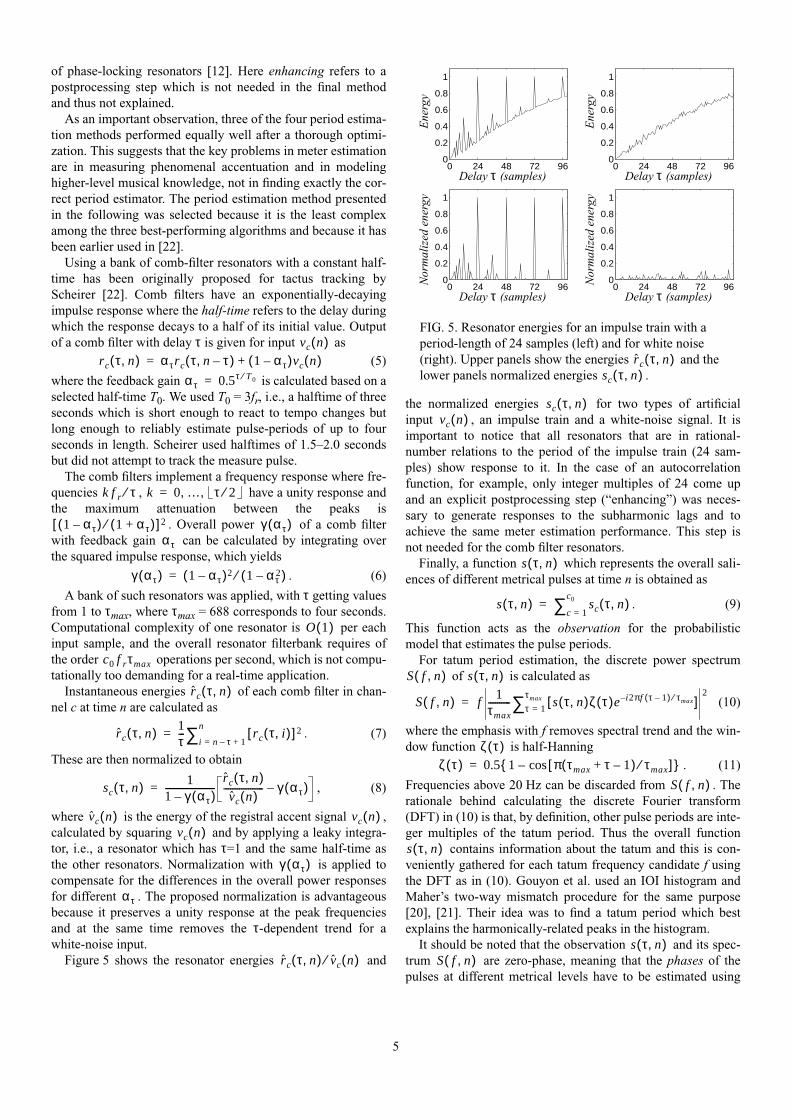
of phase-locking resonators [12]. Here enhancing refers to a
postprocessing step which is not needed in the final method
and thus not explained.
As an important observation, three of the four period estima-
tion methods performed equally well after a thorough optimi-
zation. This suggests that the key problems in meter estimation
are in measuring phenomenal accentuation and in modeling
higher-level musical knowledge, not in finding exactly the cor-
rect period estimator. The period estimation method presented
in the following was selected because it is the least complex
among the three best-performing algorithms and because it has
been earlier used in [22].
Using a bank of comb-filter resonators with a constant half-
time has been originally proposed for tactus tracking by
Scheirer [22]. Comb filters have an exponentially-decaying
impulse response where the half-time refers to the delay during
which the response decays to a half of its initial value. Output
of a comb filter with delay τ is given for input as
(5)
where the feedback gain is calculated based on a
selected half-time T0. We used T0 = 3fr, i.e., a halftime of three
seconds which is short enough to react to tempo changes but
long enough to reliably estimate pulse-periods of up to four
seconds in length. Scheirer used halftimes of 1.5–2.0 seconds
but did not attempt to track the measure pulse.
The comb filters implement a frequency response where fre-
quencies , have a unity response and
the maximum attenuation between the peaks is
. Overall power of a comb filter
with feedback gain can be calculated by integrating over
the squared impulse response, which yields
. (6)
A bank of such resonators was applied, with τ getting values
from 1 to τmax, where τmax = 688 corresponds to four seconds.
Computational complexity of one resonator is per each
input sample, and the overall resonator filterbank requires of
the order operations per second, which is not compu-
tationally too demanding for a real-time application.
Instantaneous energies of each comb filter in chan-
nel c at time n are calculated as
. (7)
These are then normalized to obtain
, (8)
where is the energy of the registral accent signal ,
calculated by squaring and by applying a leaky integra-
tor, i.e., a resonator which has τ=1 and the same half-time as
the other resonators. Normalization with is applied to
compensate for the differences in the overall power responses
for different . The proposed normalization is advantageous
because it preserves a unity response at the peak frequencies
and at the same time removes the τ-dependent trend for a
white-noise input.
Figure 5 shows the resonator energies and
the normalized energies for two types of artificial
input , an impulse train and a white-noise signal. It is
important to notice that all resonators that are in rational-
number relations to the period of the impulse train (24 sam-
ples) show response to it. In the case of an autocorrelation
function, for example, only integer multiples of 24 come up
and an explicit postprocessing step (“enhancing”) was neces-
sary to generate responses to the subharmonic lags and to
achieve the same meter estimation performance. This step is
not needed for the comb filter resonators.
Finally, a function which represents the overall sali-
ences of different metrical pulses at time n is obtained as
. (9)
This function acts as the observation for the probabilistic
model that estimates the pulse periods.
For tatum period estimation, the discrete power spectrum
of is calculated as
(10)
where the emphasis with f removes spectral trend and the win-
dow function is half-Hanning
. (11)
Frequencies above 20 Hz can be discarded from . The
rationale behind calculating the discrete Fourier transform
(DFT) in (10) is that, by definition, other pulse periods are inte-
ger multiples of the tatum period. Thus the overall function
contains information about the tatum and this is con-
veniently gathered for each tatum frequency candidate f using
the DFT as in (10). Gouyon et al. used an IOI histogram and
Maher’s two-way mismatch procedure for the same purpose
[20], [21]. Their idea was to find a tatum period which best
explains the harmonically-related peaks in the histogram.
It should be noted that the observation and its spec-
trum are zero-phase, meaning that the phases of the
pulses at different metrical levels have to be estimated using
vc n( )r c τ n,( ) ατr c τ n τ–,( ) 1 ατ–( )vc n( )+=
ατ 0.5τ T0⁄=
k f r τ⁄ k 0 … τ 2⁄, ,=
1 ατ–( ) 1 ατ+( )⁄[ ] 2 γ ατ( )ατ
γ ατ( ) 1 ατ–( )2 1 ατ2–( )⁄=
O 1( )
c0 f rτmax
r c τ n,( )
r c τ n,( ) 1τ--- r c τ i,( )[ ] 2
i n τ– 1+=
n∑=
sc τ n,( ) 11 γ ατ( )–----------------------
r c τ n,( )vc n( )
------------------ γ ατ( )–=
vc n( ) vc n( )vc n( )
γ ατ( )
ατ
r c τ n,( ) vc n( )⁄
0 24 48 72 960
0.2
0.4
0.6
0.8
1
0 24 48 72 960
0.2
0.4
0.6
0.8
1
0 24 48 72 960
0.2
0.4
0.6
0.8
1
0 24 48 72 960
0.2
0.4
0.6
0.8
1
FIG. 5. Resonator energies for an impulse train with a
period-length of 24 samples (left) and for white noise
(right). Upper panels show the energies and the
lower panels normalized energies .
r c τ n,( )sc τ n,( )
Delay τ (samples) Delay τ (samples)
Ene
rgy
Nor
mal
ized
ene
rgy
Delay τ (samples) Delay τ (samples)
Ene
rgy
Nor
mal
ized
ene
rgy
sc τ n,( )vc n( )
s τ n,( )
s τ n,( ) sc τ n,( )c 1=
c0∑=
S f n,( ) s τ n,( )
S f n,( ) f1
τmax---------- s τ n,( )ζ τ( )e i 2πf τ 1–( )– τmax⁄[ ]τ 1=
τmax∑2
=
ζ τ( )ζ τ( ) 0.5 1 π τmax τ 1–+( ) τmax⁄[ ]cos–{ }=
S f n,( )
s τ n,( )
s τ n,( )S f n,( )
5

some other source of information. As will be discussed in
Subsection D, the phases are estimated based on the states of
the comb filters, after the periods have been solved first.
C. Probabilistic model for pulse periods
Period-lengths of the metrical pulses can be estimated inde-
pendently of their phases and it is reasonable to compute the
phase only for the few winning periods. Thus the proposed
method finds periods first and then the phases (see Fig. 2).
Although estimating the phases is not trivial, the search prob-
lem is largely completed when the period-lengths have been
found.
Musical meter cannot be assumed to be static over the dura-
tion of a piece. It has to be estimated causally at successive
time instants and there must be some temporal tying between
the successive estimates. Also, the dependencies between dif-
ferent metrical pulse levels have to be taken into account. This
requires prior musical knowledge which is encoded in the
probabilistic model to be presented.
For period estimation, a hidden Markov model that describes
the simultaneous evolution of four processes is constructed.
The observable variable is the vector of instantaneous energies
of the resonators, , denoted in the following. The
unobservable processes are the tatum, tactus, and measure peri-
ods. The corresponding hidden variables are the tatum period
, tactus period , and measure period . As a mnemonic
for this notation, recall that the tatum is the temporally atomic
(A) pulse level, tactus pulse is often called “beat” (B), and
musical measure pulse is related to the harmonic (i.e., chord)
change rate (C). For convenience, we use to
denote a “meter state”, equivalent to , , and
. The hidden state process is a time-homogenous first-
order Markov which has an initial state distribution and
transition probabilities . The observable variable is
conditioned only on the current state, i.e., we have the state-
conditional observation densities .
The joint probability density of a state sequence
and observation sequence
can be written as
, (12)
where the term can be decomposed as
. (13)
It is reasonable to assume that
, (14)
i.e., given the tactus period, the tatum period does not give
additional information regarding the measure period. We fur-
ther assume that given , the other two hidden variables at
time give no additional information regarding . Here
. It follows that (13) can be written as
. (15)
Using the same assumptions, is decomposed and sim-
plified as
. (16)
The described modeling assumptions lead to a structure
which is represented as a directed acyclic graph in Figure 6.
The arrays in the graph represent conditional dependencies
between the variables. The circles denote hidden variables and
the observed variable is marked with boxes. The tactus pulse
has a central role in meter perception and it is not by chance
that the other two variables are drawn to depend on it. The
assumption in (14) is not valid if the variables are permuted.
1. Estimation of the state-conditional observation likeli-hoods
The remaining problem is to find reasonable estimates for the
model parameters, i.e., for the probabilities that appear in (12)-
(16). In the following, we ignore the time indeces for a while
for simplicity. The state-conditional observation likelihoods
are estimated from a database of musical recordings
where the musical meter has been hand-labeled. However, the
data is very limited in size compared to the number of parame-
ters to be estimated. Estimation of the state densities for each
different is impossible since each of the three dis-
crete hidden variables can take on several hundreds of different
values. By making a series of assumptions we arrive at the fol-
lowing approximation for :
. (17)
Appendix A presents the derivation of (17) and the underlying
assumptions in detail. An intuitive rationale of (17) is that a
truly existing tactus or measure pulse appears as a peak in
at the lag that corresponds to the pulse period. Analogously, the
tatum period appears as a peak in at the frequency that
corresponds to the inverse of the period. The product of these
three values correlates approximately linearly with the likeli-
hood of the observation given the meter.
2. Estimation of the transition and initial probabilities
In (15), the term can be decomposed as
, (18)
s τ n,( ) sn
τnA τn
B τnC
qn j k l, ,[ ]=τn
A j= τnB k=
τnC l=
P q1( )P qn qn 1–( )
p sn qn( )
Q q1q2…qN( )= O s1s2…sN( )=
p Q O,( ) P q1( )p s1 q1( ) P qn qn 1–( )p sn qn( )n 2=
N
∏=
P qn qn 1–( )P qn qn 1–( )
P τnB qn 1–( )P τn
A τnB qn 1–,( )P τn
C τnB τn
A qn 1–, ,( )=
P τnC τn
B τnA qn 1–, ,( ) P τn
C τnB qn 1–,( )=
τn 1–i( )
n 1– τni( )
i A B C, ,{ }∈P qn qn 1–( )
P τnB τn 1–
B( )P τnA τn
B τn 1–A,( )P τn
C τnB τn 1–
C,( )=
P q1( )
P q1( ) P τ1B( )P τ1
A τ1B( )P τ1
C τ1B( )=
q q q
n−1
n−1
n
n
n+1
n+1
n+1
n−1
B
n
B B
n−1 n n+1
n−1 n n+1
A A A
C C Cτ
τ
τ
s
τ
τ
τ
s
τ
τ
τ
s
FIG. 6. Hidden markov model for the temporal evolution
of the tatum, beat, and measure pulse periods.
p s q( )
q j k l, ,[ ]=
p s q( )p s q j k l, ,[ ]=( ) s k( )s l( )S 1 j⁄( )∝
s τ( )
S f( )
P τnA τn
B τn 1–A,( )
P τnA τn
B τn 1–A,( ) P τn
A τn 1–A( )
P τnA τn
B, τn 1–A( )
P τnA τn 1–
A( )P τnB τn 1–
A( )---------------------------------------------------------=
6
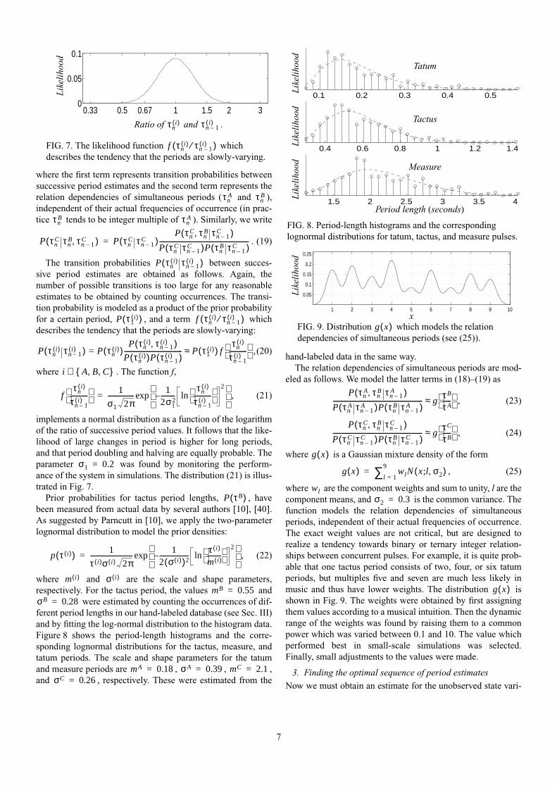
where the first term represents transition probabilities between
successive period estimates and the second term represents the
relation dependencies of simultaneous periods ( and ),
independent of their actual frequencies of occurrence (in prac-
tice tends to be integer multiple of ). Similarly, we write
. (19)
The transition probabilities between succes-
sive period estimates are obtained as follows. Again, the
number of possible transitions is too large for any reasonable
estimates to be obtained by counting occurrences. The transi-
tion probability is modeled as a product of the prior probability
for a certain period, , and a term which
describes the tendency that the periods are slowly-varying:
,(20)
where . The function f,
, (21)
implements a normal distribution as a function of the logarithm
of the ratio of successive period values. It follows that the like-
lihood of large changes in period is higher for long periods,
and that period doubling and halving are equally probable. The
parameter was found by monitoring the perform-
ance of the system in simulations. The distribution (21) is illus-
trated in Fig. 7.
Prior probabilities for tactus period lengths, , have
been measured from actual data by several authors [10], [40].
As suggested by Parncutt in [10], we apply the two-parameter
lognormal distribution to model the prior densities:
, (22)
where and are the scale and shape parameters,
respectively. For the tactus period, the values and
were estimated by counting the occurrences of dif-
ferent period lengths in our hand-labeled database (see Sec. III)
and by fitting the log-normal distribution to the histogram data.
Figure 8 shows the period-length histograms and the corre-
sponding lognormal distributions for the tactus, measure, and
tatum periods. The scale and shape parameters for the tatum
and measure periods are , , ,
and , respectively. These were estimated from the
hand-labeled data in the same way.
The relation dependencies of simultaneous periods are mod-
eled as follows. We model the latter terms in (18)–(19) as
, (23)
, (24)
where is a Gaussian mixture density of the form
, (25)
where are the component weights and sum to unity, l are the
component means, and is the common variance. The
function models the relation dependencies of simultaneous
periods, independent of their actual frequencies of occurrence.
The exact weight values are not critical, but are designed to
realize a tendency towards binary or ternary integer relation-
ships between concurrent pulses. For example, it is quite prob-
able that one tactus period consists of two, four, or six tatum
periods, but multiples five and seven are much less likely in
music and thus have lower weights. The distribution is
shown in Fig. 9. The weights were obtained by first assigning
them values according to a musical intuition. Then the dynamic
range of the weights was found by raising them to a common
power which was varied between 0.1 and 10. The value which
performed best in small-scale simulations was selected.
Finally, small adjustments to the values were made.
3. Finding the optimal sequence of period estimates
Now we must obtain an estimate for the unobserved state vari-
τnA τn
B
τnB τn
A
P τnC τn
B τn 1–C,( ) P τn
C τn 1–C( )
P τnC τn
B, τn 1–C( )
P τnC τn 1–
C( )P τnB τn 1–
C( )---------------------------------------------------------=
P τni( ) τn 1–
i( )( )
P τ1i( )( ) f τn
i( ) τn 1–i( )⁄( )
P τni( ) τn 1–
i( )( ) P τni( )( )
P τni( ) τn 1–
i( ),( )P τn
i( )( )P τn 1–i( )( )
-------------------------------------= P τ1i( )( ) f
τni( )
τn 1–i( )-----------
≈
i A B C, ,{ }∈
fτn
i( )
τn 1–i( )-----------
1
σ1 2π-----------------
12σ1
2---------
τni( )
τn 1–i( )-----------
ln2
–
exp=
σ1 0.2=
0.33 0.5 0.67 1 1.5 2 30
0.05
0.1
FIG. 7. The likelihood function which
describes the tendency that the periods are slowly-varying.
f τni( ) τn 1–
i( )⁄( )
Ratio of and .τni( ) τn 1–
i( )
Like
lihoo
d
P τB( )
p τ i( )( ) 1
τ i( )σ i( ) 2π---------------------------
12 σ i( )( )2-------------------
τ i( )
m i( )--------- ln
2–
exp=
m i( ) σ i( )
mB 0.55=σB 0.28=
mA 0.18= σA 0.39= mC 2.1=σC 0.26=
0.1 0.2 0.3 0.4 0.5
0.4 0.6 0.8 1 1.2 1.4
1.5 2 2.5 3 3.5 4
FIG. 8. Period-length histograms and the corresponding
lognormal distributions for tatum, tactus, and measure pulses.
Like
lihoo
dLi
kelih
ood
Tatum
Tactus
Measure
Period length (seconds)
Like
lihoo
d
P τnA τn
B, τn 1–A( )
P τnA τn 1–
A( )P τnB τn 1–
A( )--------------------------------------------------------- g
τB
τ A-----
≈
P τnC τn
B, τn 1–C( )
P τnC τn 1–
C( )P τnB τn 1–
C( )--------------------------------------------------------- g
τC
τB-----
≈
g x( )
g x( ) wl N x l σ2,;( )l 1=
9∑=
wlσ2 0.3=
g x( )
1 2 3 4 5 6 7 8 9 10
0.05
0.1
0.15
0.2
0.25
FIG. 9. Distribution which models the relation
dependencies of simultaneous periods (see (25)).
g x( )x
Like
lihoo
d
7

ables given the observed front-end data and the model parame-
ters. We do this by finding the most likely sequence of state
variables given the observed front-end data
. This can be straighforwardly computed
using the Viterbi algorithm widely applied in speech recogni-
tion [41]. Thus, we seek the sequence of period estimates,
(26)
where denotes the joint probability density of the
hidden and observed variables, as defined in (12).
For the Viterbi-decoding, we need to define the quantity
, (27)
which is the best score along a single path at time n, which
takes into account the first n observations and ends in state
. By induction we then compute
(28)
In a causal model, the meter estimate at time n is deter-
mined according to the end-state of the best partial path at that
point in time. A noncausal estimate after seeing a complete
sequence of observations can be computed using backward
decoding, and
. (29)
The inequality is due to “pruning” some of the path candidates
by evaluating only a subset of best path candidates at each time
instant, and thus the resulting path is not necessarily the global
optimum. However, in practice the difference is small. Evaluat-
ing all the possible path candidates would be computationally
very demanding. Therefore, we apply a suboptimal beam-
search strategy, and evaluate only a predefined number of the
most promising path candidates at each time instant. The selec-
tion of the most promising candidates is made using a greedy
selection strategy. Once in a second, we select independently
best candidates for the tatum, tactus, and measure periods.
The number of candidates was found to be safe and
was used in simulations. The selection is made by maximizing
for . After selecting the best
candidates for each, we need only to compute the observation
likelihoods for meter candidates, i.e., for the differ-
ent combinations of the tatum, tactus, and measure periods.
This is done according to Eq (17) and the results are stored into
a data vector. The transition probabilities are computed using
Eq. (15) and stored into a 125-by-125 matrix. These data struc-
tures are then used in the Viterbi algorithm.
D. Phase estimation
The phases of the three pulses are estimated at successive time
instants, after the periods have been decided at these points. We
use , to refer to the estimated periods of the
tatum, tactus, and measure pulses at time n, respectively. The
corresponding phases of the three pulses, , are expressed as
“temporal anchors”, i.e., time values when the nearest beat unit
occurs with respect to the beginning of a piece. Periods and
phases, and , completely define the meter at time n.
In principle, the phase of the measure pulse, , determines
the phase of all the three levels. This is because in a well-
formed meter, each measure-level beat must coincide with a
beat at all the lower metrical levels. However, determining the
phase of the measure pulse is difficult and turned out to require
pattern recognition techniques, whereas tactus phase estima-
tion is more straightforward and robust. We therefore propose a
model where the tactus and measure phases are estimated sepa-
rately using two parallel models. For the tatum pulse, phase
estimation is not needed but the tactus phase can be used.
Scheirer has proposed using the state vectors of comb filters
to determine the phase of the tactus pulse [22]. This is equiva-
lent to using the latest outputs of a resonator with delay .
We have resonators at several channels c and, consequently, an
output matrix where is the channel
index and the phase index j takes on values between
and n when estimation is taking place at time n. For conven-
ience, we use to denote the output matrix of a
found pulse period and the notation to refer to
the individual elements of . The matrix acts as the
observation for phase estimation at time n.
Fig. 10 shows an example of the observation matrix
when tactus phase estimation is taking place 20 seconds after
the beginning of a piece. The four signals at different channels
are the outputs of the comb filter which corresponds to the esti-
mated tactus period = 0.51 seconds. The output matrix
contains the latest 0.51 seconds of the output signals, as indi-
cated with the rectangle. The correct phase value has been
marked with a dashed line. As discussed in Sec. II.B, comb fil-
ters implement a “harmonic” frequency response and therefore
the outputs show clear periodicity with period .
Two separate hidden Markov models are evaluated in paral-
lel, one for the tactus phase and another for the measure phase.
No joint estimation is attempted. The two models are very sim-
ilar and differ only in how the state-conditional observation
densities are defined. In both models, the observable variable is
the output matrix of the resonator which corresponds
to the found pulse period. The hidden variable is the phase of
the pulse, , taking on values between and n.
The hidden state process is a time-homogenous first-order
Markov which has an initial state distribution and tran-
sition probabilities . The observable variable is
conditional only on the current state, thus we have the state-
Q q1q2…qN( )=O s1s2…sN( )=
Q maxQ
p Q O,( )[ ]arg=
p Q O,( )
δn j k l, ,( ) maxq1…qn 1–
P q1…qn 1– qn j k l, ,[ ] s1…sn,=,( )=
qn j k l, ,[ ]=
δn 1+ j k l, ,( ) p sn 1+ qn 1+ j k l, ,[ ]=( )
maxj ′ k′ l ′, ,
δn j ′ k′ l ′, ,( )P qn 1+ j k l, ,[ ]= qn j ′ k′ l ′, ,[ ]=( )[ ]⋅
=
qn
maxj k l, ,
δn j k l, ,( )[ ] maxQ
p Q O,( )[ ]≈
KK 5=
p τni( )( )P sn τn
i( )( ) i A B C, ,{ }=
K 3 125=
τni( ) i A B C, ,{ }∈
ϕni( )
τni( ) ϕn
i( )
ϕnC
τ τ
r c τ j,( ) c 1 2 … c0, , ,=n τ 1+–
Rni( ) r c τn
i( ) j,( )τn
i( ) Rni( )( )c j,
Rni( ) Rn
i( )
18.6 18.8 19 19.2 19.4 19.6 19.8
1234
nn−τBn
φBn
FIG. 10. The rectangle indicates the observation matrix
for tactus phase estimation at time n (here period is
0.51 s.). Dashed line shows the correct phase in this case.
RnB
τnB
Time (seconds)
Cha
nnel
c
RnB
τnB Rn
B
ϕnB
τnB
Rni( ) τn
i( )
ϕni( ) n τn
i( ) 1+–
P ϕ1( )P ϕn ϕn 1–( )
8

conditional observation densities .
Again, the remaining problem is to find reasonable estimates
for the model parameters. State-conditional observation likeli-
hoods for the tactus pulse are approximated as
. (30)
It is, the likelihood is proportional to a weighted sum of the
resonator outputs across the channels. The exact weights of the
different channels are not critical. Across-band summing is
intuitively meaningful and earlier used in [22] and [35].
Emphasizing the low frequencies is motivated by the “stable
bass” rule, as stated by Lerdahl and Jackendoff in [1], and
improved the robustness of phase estimation in simulations.
For the purpose of estimating the measure pulse phase, a for-
mula for the state-conditional observation likelihoods analo-
gous to that in (30) is derived, but so that different channels are
weighted and delayed in a more complex manner. It turned out
that pattern matching of some form is necessary to analyze
music at this time scale and to estimate the measure phase
based on the output matrix . It is, no simple formula such as
(30) exists. In the case that the system would have access to the
pitch content of an incoming piece, the points of harmonic
change might serve as cues for estimating the measure phase in
a more straightforward manner. However, this remains to be
proved. Estimation of the higher-level metrical pulses in audio
data has been earlier attempted by Goto and Muraoka, who
resorted to pattern matching [17] or to straightforward chord
change detection [18]. The method presented in the following
is the most reliable that we found.
First, a vector is constructed as
, (31)
where
, (32)
, (33)
and (x mod y) denotes modulus after division. Scalars are
weights for the resonator outputs at channels c and with delays
k. The weights encode a typical pattern of energy fluctua-
tions withing one measure period and are estimated so that the
maximum of indicates the measure phase. Two univer-
sally applicable patterns and were found, leading to
the corresponding vectors and . The values of
these matrices are given in Appendix B. Both patterns can be
characterized as a pendulous motion between a low-frequency
event and a high-intensity event. The first pattern can be sum-
marized as “low, loud, –, loud”, and the second as “low, –
, loud, –”. The two patterns are combined into a single vector
to perform phase estimation according to whichever pattern
matches better to the data
. (34)
The state-conditional observation likelihoods are then defined
as
. (35)
Other pattern matching approaches were evaluated, too. In
particular, we attempted to sample at the times of the tac-
tus beats and to train statistical classifiers to choose the beat
which corresponds to the measure beat (see [42] for further
elaboration on this idea). However, the methods were basically
equivalent to that described above, yet less straightforward to
implement and performed slightly worse.
Transition probabilities between successive
phase estimates are modeled as follows. Given two phase esti-
mates (i.e., beat occurrence times), the conditional probability
which ties the successive estimates is assumed to be normally
distributed as a function of a prediction error e which measures
the deviation of from a predicted next beat occurence time
given the previous beat time and the period :
(36)
where
, (37)
and is common for . In (37), it should be
noted that none or several periods may elapse between
and . The initial state distribution is assumed to be
uniformly distributed, i.e., for all j.Using (30), (35), and (36), causal and noncausal computa-
tion of phase is performed using the Viterbi algorithm as
described in Sec II.C. Fifteen phase candidates for both the
winning tactus and the winning measure period are generated
once in a second. The candidates are selected in a greedy man-
ner by picking local maxima in . The corre-
sponding probability values are stored into a vector and
transition probabilities between successive estimates are com-
puted using (36).
E. Sound onset detection and extrametrical events
Detecting the beginnings of discrete acoustic events one-by-
one has many uses. It is often of interest whether an event
occurs at a metrical beat or not, and what is the exact timing of
an event with respect to its ideal metrical position. Also, in
some musical pieces there are extrametrical events, such as tri-plets, where an entity of e.g. four tatum periods is exception-
ally divided into three parts, or grace notes which are pitch
events that occur a bit before a metrically stable event.
In this paper, we used an onset detector as a front-end to one
of the reference systems (designed for symbolic MIDI input) to
enable it to process acoustic signals. Rather robust onset detec-
tion is achieved by using an overall accent signal which
is computed by setting in (4). Local maxima in
represent onset candidates and the value of at these
points reflects the likelihood that a discrete event occurred. A
simple peak-picking algorithm with a fixed threshold level can
then be used to distinguish genuine onsets from the changes
and modulations that take place during the ringing of a sound.
p Rni( ) ϕn
i( )( )
p RnB ϕn
B( )
p RnB ϕn
B j=( ) c0 c– 2+( ) RnB( )c j,
c 1=
c0
∑∝
ϕnC
RnC
hn l( )
hn l( ) ηc k, RnC( )c j k l n, ,( ),
k 0=
3
∑c 1=
c0
∑=
l 0 1 … τnC 1–, , ,=
j k l n, ,( ) n τnC– 1 l
kτnC
4---------+
mod τnC
+ +=
ηc k,
ηc k,
hn l( )ηc k,
1( ) ηc k,2( )
hn1( ) l( ) hn
2( ) l( )
hn1 2,( ) l( ) max hn
1( ) l( ) hn2( ) l( ),{ }=
p RnC ϕn
C j=( ) hn1 2,( ) j n τn
C– 1+( )–( )∝
RnC
P ϕni( ) ϕn 1–
i( )( )
ϕni( )
ϕn 1–i( ) τn
i( )
P ϕni( ) ϕn 1–
i( )( ) 1
σ3 2π-----------------
e2
2σ32
---------–
exp=
e1
τni( )------- ϕn
i( ) ϕn 1–i( )–
τni( )
2-------+
mod τni( ) τn
i( )
2-------–
=
σ3 0.1= i B C,{ }∈ϕn 1–
i( )
ϕni( ) P ϕ1( )
P ϕ1i( ) j=( ) 1 τn
i( )⁄=
p Rni( ) ϕn
i( ) j=( )
v n( )m0 b0= v n( )
v n( )
9

III. RESULTS
This section will look at the performance of the proposed
method in simulations. The results will be compared with those
of two reference systems. The distribution of errors will be
analyzed and the importance of different processing elements
will be validated.
A. Experimental setup
Table 1 shows the statistics of the database that was used to
evaluate the accuracy of the proposed meter estimation method
and the two reference methods. Musical pieces were collected
from CD recordings, downsampled to a single channel, and
stored to a hard disc using 44.1 kHz sampling rate and 16 bit
resolution.The database was created for the purpose of musical
signal classification in general, and the balance between genres
is according to an informal estimate of what people listen to.
The metrical pulses were manually annotated for approxi-
mately one-minute long excerpts which were selected to repre-
sent each piece. Tactus and measure pulse annotations were
made by a musician who tapped along with the pieces. The tap-
ping signal was recorded and the tapped beat times were then
detected semiautomatically. The tactus pulse could be anno-
tated for 474 of a total of 505 pieces. The measure pulse could
be reliably marked by listening for 320 pieces. In particular,
annotation of the measure pulse was not attempted for classical
music without the musical scores. Tatum pulse was annotated
by the first author by listening to the pieces together with the
annotated tactus pulse and by determining the integer ratio
between the tactus and the tatum period lengths. The integer
ratio was then used to interpolate the tatum beats between the
tapped tactus beats.
Evaluating a meter estimation system is not trivial. The issue
has been addressed in depth by Goto and Muraoka in [19]. As
suggested in [19], we use the longest continuous correctly esti-
mated segment as a basis for measuring the performance. This
means that one inaccuracy in the middle of a piece leads to
50 % performance. The longest continuous sequence of correct
pulse estimates in each piece is sought and compared to the
length of the segment which was given to be analyzed. The
ratio of these two lengths determines the performance rate for
one piece and these are then averaged over all pieces. However,
prior to the meter analysis, all the algorithms under considera-
tion were given a four-second “build-up period” in order to
make it theoretically possible to estimate the correct period
immediately from the beginning of the evaluation segment.
Also, it was taken care that any of the input material did not
involve tempo discontinuities. More specifically, the interval
between two tapped reference beat times (pulse period) does
not change more than 40% at a time, between two successive
beats. Other tempo fluctuations were naturally allowed.
A correct period estimate is defined to deviate less than
17.5 % from the annotated reference and a correct phase to
deviate from an annotated beat time less than 0.175 times the
annotated period length. This precision requirement has been
suggested in [19] and was found appropriate here since inaccu-
racies in the manually tapped beat times allow meaningful
comparison of only up to that precision. However, for the
measure pulse, the period and phase requirements were tight-
ened to 10 % and 0.1, because the measure period-lengths are
large and thus more accurate evaluation is possible – and also
necessary as will be seen. For the tatum pulse, tactus phase is
used and thus the phase is correct always when the tactus phase
is correct, and only the period has to be considered separately.
Performance rates are given for three different criteria [19]:
• “Correct”: A pulse estimate at time n is accepted if both its
period and phase are correct.
• “Accept d/h”: A pulse estimate is accepted if its phase is
correct and the period matches either 0.5, 1.0, or 2.0 times
the annotated reference. It is, period doubling or halving is
accepted but the factor must not change within the continu-
ous sequence. Correct meter estimation takes place, but a
wrong metrical level is chosen to be e.g. the tactus pulse.
• “Period correct”: A pulse estimate is accepted if its period
is correct. Phase is ignored. For tactus, this is interpreted as
the tempo estimation performance.
Which is the single best number to characterize the perform-
ance of a pulse estimator? This was investigated by auralizing
meter estimation results. It was observed that temporal conti-
nuity in producing correct estimates is indeed aurally impor-
tant. Secondly, phase errors are very disturbing. Third, period
doubling or halving is not very disturbing. Tapping consistentlytwice too fast or slow does not matter much. Moreover, select-
ing the correct metrical level is in some cases ambiguous even
for a human listener, especially in the case of the tatum pulse.
In summary, it appears that the “accept d/h” criterion gives a
single best number to characterize the performance of a sys-
tem.
B. Reference systems
To put the results in perspective, two reference methods are
used as a baseline in simulations. This is essential because the
principle of using a continuous sequence of correct estimates
for evaluation gives a somewhat pessimistic picture of the
absolute performance.
The methods of Scheirer [22] and Dixon [16] are very differ-
ent, but both systems represent the state-of-the-art in tactus
pulse estimation and their source codes are publicly available.
Here, the used implementations and parameter values were
those of the original authors. However, for Scheirer’s method,
some parameter tuning was made which slightly improved the
results. Dixon developed his system primarily for MIDI-input,
Table 1: Statistics of the evaluation database.
Genre# Pieces with annotated metrical pulses
tatum tactus measure
Classical 69 84 0
Electronic / dance 47 66 62
Hip hop / rap 22 37 36
Jazz / blues 70 94 71
Rock / pop 114 124 101
Soul / RnB / funk 42 54 46
Unclassified 12 15 4
Total 376 474 320
10

and provided only a simple front-end for analyzing acoustic
signals. Therefore, a third system denoted “O + Dixon” was
developed where an independent onset detector (described in
Sec. II.E), was used prior to Dixon’s tactus analysis. System-
atic phase errors were compensated for in both methods.
C. Experimental results
In Table 2 the tactus tracking performance of the proposed
causal and noncausal algorithms is compared with those of the
two reference methods. As the first observation, it was noticed
that the reference methods did not maintain the temporal conti-
nuity of acceptable estimates. For this reason, the performance
rates are also given as percentages of individual acceptable
estimates (right half of Table 2). Dixon’s method has difficul-
ties in choosing the correct metrical level for tactus, but per-
forms well according to the “accept d/h” criterion when
equipped with the new onset detector. The proposed method
outperforms the previous systems in both accuracy and tempo-
ral stability.
Table 3 shows the meter estimation performance for the pro-
posed causal and noncausal algorithms. As for human listeners,
meter estimation seems to be easiest at the tactus pulse level.
For the measure pulse, period estimation can be done robustly
but estimating the phase is difficult. A reason for this is that in
a large part of the material, two rhythmic patterns elapse within
one measure period, and the system has difficulties in choosing
which one is the first. In the case that π-phase errors (each beat
is displaced by a half-period) would be accepted, the perform-
ance rate would be essentially the same as for the tactus. How-
ever, π-phase errors are disturbing and should not be accepted.
For the tatum pulse, in turn, deciding the period is difficult.
This is because the temporally atomic pulse rate typically
comes up only occasionally, making temporally stable analysis
hard to attain. The method often has to halve its period hypoth-
esis when the first rapid event sequence occurs. This appears in
the performance rates so that the method is not able to produce
a consistent tatum period over time but alternates between e.g.
the reference and double the reference. This degrades the tem-
porally continuous rate, although the “accept d/h” rate is very
good for individual estimates. The produced errors are not very
disturbing when listening to the results.
Figure 11 shows the “accept d/h” (continuity required) per-
formance rates for different musical genres. For classical
music, the proposed method is only moderately successful,
although e.g. the tactus rate still outperforms the performance
of the reference methods for the whole material. However, this
may suggest that pitch analysis would be needed to analyze the
meter in classical music. In jazz music, the complexity of
musical rhythms is higher on the average and the task thus
harder.
In Figure 12, the temporal precision of the proposed method
is illustrated. We measured the time deviation of accepted
phase estimates from the annotated beat times. The deviation is
expressed in relation to the annotated period-length. The histo-
gram shows the distribution of deviation values. It should be
noted that the reference tapping is not absolutely accurate, but
the histogram reflects inaccuracies in both. For the measure
pulse, the histogram is quite exactly a 3.8-times narrower copy
of that for the tactus. Thus the absolute time deviations are
roughly the same, suggesting that they are mostly due to the
reference tapping. The dashed line in the right-hand side histo-
Table 2: Tactus estimation performance (%) of different methods.
Method
Continuity required Individual estimates
correctaccept
d/h
period
correctcorrect
accept
d/h
period
correct
Causal 57 68 74 63 78 76
Noncausal 59 73 74 64 80 75
Scheirer [22] 27 31 30 48 69 57
Dixon [16] 7 26 10 15 53 25
O + Dixon 12 39 15 22 63 30
Table 3: Meter estimation performance for the proposed method.
Method Pulse
Continuity required Individual estimates
correctaccept
d/h
period
correctcorrect
accept
d/h
period
correct
Causal tatum 44 57 62 51 72 65
tactus 57 68 74 63 78 76
measure 42 48 78 43 51 81
Non-
causal
tatum 45 63 62 52 74 65
tactus 59 73 74 64 80 75
measure 46 54 79 47 55 81
0 20 40 60 80 100
soul/RnB/funk
rock / pop
jazz
hip hop / rap
electr. / dance
classical
FIG. 11. Performance within different musical genres. The
“accept d/h” (continuity required) percentages are shown for
the tatum (white), tactus (gray), and measure (black) pulses.
%
−0.2 −0.1 0 0.1 0.20
0.05
0.1
−0.2 −0.1 0 0.1 0.20
0.1
0.2
0.3
0.4
FIG. 12. Relative occurrence frequencies of different phase
deviations from the reference phase. The deviation is
measured in relation to the period length for the tactus (left)
and measure pulse (right).
Relative deviation Relative deviation
Occ
urre
nce
rate
Occ
urre
nce
rate
11

gram shows the histogram if deviations of up to 0.175 times the
period would be accepted for the measure pulse. It is, rhythmi-
cally confused phase estimates would be accepted. Therefore, a
higher precision (0.1) was required for the measure phase.
Figure 13 shows histograms where the ratio of the estimated
period and the annotated period was measured. As can be seen,
almost all period estimation errors are either half or double the
correct period. In the case that the phase is ignored, 83 %
(tatum), 88 % (tactus), and 91 % (measure) of the period esti-
mates are either correct, half, or double the reference period.
The fact that the measure pulse could not be annotated for clas-
sical music explains why the measure period estimation rate is
higher than that of the tactus.
D. Importance of different parts
Table 4 gives the performance rates for different system config-
urations. Different elements of the proposed model were disa-
bled in order to evaluate their importance. In each case, the
system was kept otherwise fixed. The baseline method is the
noncausal system, as in Table 3.
In the first test, the dependencies between the different pulse
levels were broken by using a non-informative (flat) distribu-
tion for in (25). This slightly degrades the performance in
all cases. In the second test, the dependencies between tempo-
rally successive estimates were broken by using a non-informa-
tive distribution for the transition probabilities between
successive period and phase estimates, and
, respectively. This degrades the temporal stabil-
ity of the estimates considerably and hence collapses the per-
formance rates which use the longest continuous correct
segment for evaluation. In the third case, the both types of
dependencies were broken. The system still performs moder-
ately, indicating that the initial time-frequency analysis method
and the comb-filter resonators provide a rather high level of
robustness as such.
IV. CONCLUSIONS
A method has been described which can successfully estimate
the meter of acoustic musical signals. Musical genres of very
diverse types can be processed with a common system configu-
ration and parameter values. For most musical material, rela-
tively low-level acoustic information can be used, without the
need to model the higher-level auditory functions such as
sound source separation or multipitch analysis.
Similarly to human listeners, computational meter estima-
tion is easiest at the tactus pulse level. For the measure pulse,
period estimation can be done equally robustly but estimating
the phase is less straightforward. Either pattern recognition
techniques or pitch analysis seems to be needed to analyze
music at this time scale. For the tatum pulse, in turn, phase esti-
mation is not difficult at all, but deciding the period is very dif-
ficult for both humans and a computational algorithm. This is
because the temporally atomic pulse rate typically comes up
only occasionally. Thus causal processing is difficult and it is
often necessary to halve the tatum hypothesis when the first
rapid event sequence occurs.
The critical elements of a meter estimation system appear to
be the initial time-frequency analysis part which measures
musical accentuation as a function of time and the (often
implicit) internal model which represents primitive musical
knowledge. The former is needed to provide robustness for
diverse instrumentations in e.g. classical, rock, or electronic
music. The latter is needed to achieve temporally stable meter
tracking and to fill in parts where the meter is only faintly
implied by the musical surface. A challenge in the latter part is
to develop a model which is generic for various genres, for
example for jazz and classical music. The proposed model
describes sufficiently low-level musical knowledge to general-
ize over different genres.
The presented method enables both causal and noncausal
processing within the same model. The backward decoding
strategy in the Viterbi algorithm acts as a satisfying counterpart
of a phenomenon called revision in human perception. Here
revision refers to the manner in which the interpretation of pre-
vious material is affected by what happens afterwards. Back-
ward decoding at successive time instants is not
computationally demanding and gives a retrospective estimate
over the whole history up to that point.
APPENDIX A: DERIVATION OF OBSERVATION DENSITIES
This appendix presents the derivation and underlying assump-
tions in the estimation of the state-conditional observation like-
lihoods . We first assume the realizations of
independent of the realizations of and :
(38)
This violates the dependencies of our model but significantly
simplifies the computations and makes it possible to obtain rea-
sonable estimates. Furthermore, tatum information is most
clearly visible in the spectrum of the resonator outputs, thus we
use
, (39)
0.5 1 20
0.2
0.4
0.5 1 20
0.2
0.4
0.6
0.5 1 20
0.2
0.4
0.6
0.8
FIG. 13. Histogram of period-estimation errors for tatum,
tactus, and measure pulses, from left to right, respectively.
Occ
urre
nce
rate
Ratio of estimated period to reference period
Table 4: Meter estimation performance (%) for different system
configurations
Method
Require continuity,
accept d/h
Individual estimates,
accept d/h
tatum tactus measure tatum tactus measure
0. Baseline 62 73 54 74 80 55
1. No joint estim. 58 68 49 71 75 50
2. No temporal proc. 45 54 31 72 77 50
3. Neither of the two 41 50 25 70 72 44
g x( )
P τni( ) τ i( )
n 1–( )P ϕn
i( ) ϕn 1–i( )( )
p s q( ) τ A
τB τC
P s τ A j τB k τC l=,=,=( )P s τB k τC l=,=( )P s τ A j=( )∝
P s τ A j=( ) P S τ A j=( )=
12

where S is the spectrum of s, according to (10). We further
assume the components of s and S to be conditionally inde-
pendent of each other given the state, and write
(40)
It is reasonably safe to make two more simplifying assump-
tions. First, we assume that the height of s and S at the lags cor-
responding to a period actually present in the signal depend
only on the particular period, not on other periods. Second, the
value at a lag where there is no period present in the signal is
independent of the true periods , and , and is domi-
nated by the fact that no period corresponds to that particular
lag. Hence, (40) can be written as
(41)
where denotes the probability of value
given that is a tactus pulse period and
denotes the probability of value given that is not a tac-
tus pulse period. These conditional probability distributions
(tactus, measure, and tatum each have two distributions) were
approximated by discretizing the value range of
and by calculating a histogram of values in the cases that
is or is not an annotated metrical pulse period.
Then, by defining
(42)
Equation (41) can be written as
(43)
where the scalar is a function of s but does not depend on
q.
By using the two approximated histograms for tactus, meas-
ure, and tatum, each of the three terms of the form
in (43) can be represented
as a single discrete histogram. These were modeled as first
order polynomials. The first two terms depend linearly on the
value and the last term depends linearly on the value
. Thus we can write
. (44)
The histograms could be more accurately modeled with third-
order polynomials, but this did not bring performance advan-
tage over the simple linear model in (44).
APPENDIX B
Numerical values of the matrices used in Sec. II.D:
, , (45)
where channel c determines the row and delay k the column.
The first row correspond to the lowest-frequency channel.
V. REFERENCES
[1] F. Lerdahl, R. Jackendoff, A Generative Theory of TonalMusic. MIT Press, Cambridge, Massachusetts, 1983.
[2] E. F. Clarke, “Rhythm and Timing in Music,” In The Psy-chology of Music, D. Deutsch, Ed., Academic Press, 1999.
[3] J. Bilmes, “Timing is of the Essence: Perceptual and
Computational Techniques for Representing, Learning,
and Reproducing Expressive Timing in Percussive
Rhythm,” M.Sc. thesis, Massachusetts Institute of Tech-
nology, 1993.
[4] C. S. Lee, “The perception of metrical structure: experi-
mental evidence and a model,” In Representing musicalstructure, P. Howell, R. West, and I. Cross, Eds., Aca-
demic Press, London, 1991.
[5] M. J. Steedman, “The perception of musical rhythm and
metre,” Perception (6), pp. 555-569, 1977.
[6] H. C. Longuet-Higgins, C. S. Lee, “The perception of
musical rhythms,” Perception (11), pp. 115-128, 1982.
[7] C. S. Lee, “The rhythmic interpretation of simple musical
sequences: towards a perceptual model,” In MusicalStructure and Cognition, I. Cross, P. Howell, and R. West
Eds., Academic Press, London, 1985.
[8] D. J. Povel, P. Essens, “Perception of temporal patterns,”
Music Perception 2 (4), pp. 411-440, 1985.
[9] P. Desain, H. Honing, “Computational Models of Beat
Induction: The Rule-Based Approach,” Journal of NewMusic Research, Vol. 28, No. 1, pp. 29-42, 1999.
[10] R. Parncutt, “A Perceptual Model of Pulse Salience and
Metrical Accent in Musical Rhythms,” Music Perception,
Vol. 11, No. 4, pp. 409-464, Summer 1994.
[11] J. C. Brown, “Determination of the meter of musical
scores by autocorrelation,” J. Acoust. Soc. Am. 94, pp.
1953-1957, 1993.
[12] E. W. Large, J. F. Kolen, “Resonance and the perception
of musical meter”. Connection science, 6 (1), pp. 177-
208, 1994.
[13] D. F. Rosenthal, “Machine rhythm: Computer emulation
of human rhythm perception,” Ph.D. thesis, Massachu-
setts Institute of Technology, 1992.
[14] P. E. Allen, R. B. Dannenberg, “Tracking Musical Beats
in Real Time,” In Proc. International Computer MusicConference, San Francisco, 1990.
[15] D. Temperley, Cognition of Basic Musical Structures.
MIT Press, Cambridge, Massachusetts, 2001.
[16] S. Dixon, “Automatic Extraction of Tempo and Beat from
Expressive Performances,” J. New Music Research 30 (1),
pp. 39-58, 2001.
[17] M. Goto, Y. Muraoka, “Music understanding at the beat
P s τB k τC l=,=( )P S τ A j=( )
P s k'( ) τB k τC l=,=( )k' 1=
τmax
∏ P S 1 j '⁄( ) τ A j=( )j ' 1=
τmax
∏=
τB τC, τA
P s q j k l, ,[ ]=( )
P s k( ) τB k=( )P s l( ) τC l=( ) P s k′( ) τB τC k'≠,( )k′ k l,≠∏
P S 1 j⁄( ) τ A j=( ) P S 1 j ′⁄( ) τ A j '≠( )j ′ j≠∏⋅
=
P s τ( ) τB τ=( ) s τ( )τ P s τ( ) τB τ≠( )
s τ( ) τ
s τ( ) 0 1,[ ]∈s τ( )
τ
β s( ) P s k'( ) τB τC, k'≠( )k' 1=
τmax
∏ P S1j '---
τ A j '≠
j ' 1=
τmax
∏=
P s q j k l, ,[ ]=( ) β s( )
P s k( ) τB k=( )P s k( ) τB τC, k≠( )---------------------------------------------⋅
P s l( ) τC l=( )P s l( ) τB τC, l≠( )------------------------------------------
P S 1 j⁄( ) τ A j=( )P S 1 j⁄( ) τ A j≠( )--------------------------------------------
=
β s( )
P s τ( ) τ i( ) τ=( ) P s τ( ) τ i( ) τ≠( )⁄
s τ( )S 1 τ⁄( )
p s q j k l, ,[ ]=( ) s k( )s l( )S 1 j⁄( )∝
ηc k,1( )
12 1.0 0 5.7
0 2.0 0 2.0
0 3.0 0 3.0
0 4.0 0 4.0
= ηc k,2( )
10 0 1.4 1.3
0 0 2.8 0.8
0 0 4.3 1.2
0 0 5.8 1.5
=
13

level — real-time beat tracking for audio signals,” In
Working Notes of the IJCAI-95 Workshop on Computa-tional Auditory Scene Analysis, 1995, pp. 68-75.
[18] M. Goto, Y. Muraoka, “Real-time Rhythm Tracking for
Drumless Audio Signals — Chord Change Detection for
Musical Decisions,” In Proc. IJCAI-97 Workshop onComputational Auditory Scene Analysis, 1997, pp. 135-
144.
[19] M. Goto, Y. Muraoka, “Issues in Evaluating Beat Track-
ing Systems,” IJCAI-97 Workshop on Issues in AI andMusic, 1997, pp. 9-16.
[20] F. Gouyon, P. Herrera, P., Cano, “Pulse-dependent analy-
ses of percussive music,” In Proc. AES 22nd InternationalConference on Virtual, Synthetic and EntertainmentAudio, Espoo, Finland, June 2002, pp. 396-401.
[21] R. C. Maher, J. W. Beauchamp, “Fundamental frequency
estimation of musical signals using a two-way mismatch
procedure,” J. Acoust. Soc. Am. 95 (4), pp. 2254-2263,
1994.
[22] E. D. Scheirer, “Tempo and beat analysis of acoustic
musical signals,” J. Acoust. Soc. Am. 103 (1), pp. 588-601,
1998.
[23] W. A. Sethares, T. W. Staley, “Meter and Periodicity in
Musical Performance,” Journal of New Music ResearchVol. 22, No. 5, 2001.
[24] A. T. Cemgil, B. Kappen, “Monte Carlo Methods for
Tempo Tracking and Rhythm Quantization,” Journal ofArtificial Intelligence Research 18, pp. 45-81, 2003.
[25] C. Raphael, “Automated Rhythm Transcription,” In Proc.International Symposium on Music Information Retrieval,Indiana, Oct. 2001, pp. 99-107.
[26] J. Laroche, “Estimating tempo, swing and beat locations
in audio recordings,” In Proc. Workshop on Applicationsof Signal Processing to Audio and Acoustics, New Paltz,
New York, Oct. 2001, pp. 135-138.
[27] A. P. Klapuri, “Sound onset detection by applying psy-
choacoustic knowledge,” In Proc. IEEE InternationalConference on Acoustics, Speech, and Signal Processing,
Phoenix, Arizona, 1999, pp. 3089-3092.
[28] D. Moelants, C. Rampazzo, “A Computer System for the
Automatic Detection of Perceptual Onsets in a Musical
Signal,” In KANSEI - The Technology of Emotion, A.
Camurri, Ed., Genova: AIMI/DIST, 1997, pp. 141-146.
[29] M. Davy, S. Godsill, “Detection of Abrupt Spectral
Changes using Support Vector Machines. An application
to audio signal segmentation,” In Proc. IEEE Interna-
tional Conference on Acoustics, Speech, and SignalProcessing, Orlando, Florida, May 2002, pp. 1313-1316.
[30] M. Marolt, A. Kavcic, M. Privosnik, “Neural Networks
for Note Onset Detection in Piano Music,” In Proc. Inter-national Computer Music Conference, Göteborg, Sweden,
Sep. 2002.
[31] S. A. Abdallah, M. D Plumbley, “Probability as metadata:
Event detection in music using ICA as a conditional den-
sity model,” In Proc. 4th International Symposium onIndependent Component Analysis and Blind Signal Sepa-ration, Nara, Japan, April 2003.
[32] C. Duxbury, J. P. Bello, M. Davies, M. Sandler, “Complex
domain onset detection for musical signals,” In Proc. 6thInt. Conf. on Digital Audio Effects, London, UK, Sep.
2003.
[33] A. P. Klapuri, “Multiple Fundamental Frequency Estima-
tion Based on Harmonicity and Spectral Smoothness,”
IEEE Trans. Speech and Audio Processing, 11(6), pp.
804–816, Nov. 2003.
[34] J. K. Paulus, A. P. Klapuri, “Conventional and periodic N-
grams in the transcription of drum sequences,” In Proc.IEEE International Conference on Multimedia and Expo,
Baltimore, Maryland, July 2003.
[35] R. Meddis and M. J. Hewitt, “Virtual pitch and phase sen-
sitivity of a computer model of the auditory periphery.
I: Pitch identification,” J. Acoust. Soc. Am. 89 (6), pp.
2866–2882, 1991.
[36] B. R. Glasberg, B. C. J. Moore, “Derivation of Auditory
Filter Shapes from Notched-Noise Data,” Hear. Res., Vol.
47, pp. 103-138, 1990.
[37] B. J. C. Moore, Ed., Hearing. Handbook of Perceptionand Cognition (2nd edition). Academic Press Inc., 1995.
[38] R. Meddis, “Simulation of mechanical to neural transduc-
tion in the auditory receptor,” J. Acoust. Soc. Am. 79 (3),
pp. 702-711, March 1986.
[39] A. de Cheveigné and H. Kawahara, “YIN, a fundamental
frequency estimator for speech and music,” J. Acoust. Soc.Am. 111 (4), pp. 1917-1930, April 2002.
[40] L. van Noorden, D. Moelants, “Resonance in the Percep-
tion of Musical Pulse,” Journal of New Music Research,
Vol. 28, No. 1, pp. 43-66, 1999.
[41] L. R. Rabiner, B.–H. Juang, Fundamentals of Speech Rec-ognition. Prentice-Hall, New Jersey, 1993.
[42] Jarno Seppänen, “Computational models of musical meter
recognition,” M.Sc. thesis, Tampere University of Tech-
nology, Tampere, Finland, 2001.
14
