signal processing over graphs: distributed optimization...

Signal Processing over Graphs: Distributed Optimization and

Bio-Inspired Mechanisms

Sergio Barbarossa

1 22/06/15 Università di Siena – June 2015

Overall summary 1. Algebraic graph theory 2. Signal Processing over Graphs 3. Distributed OpFmizaFon over Networks 4. Examples of OpFmizaFon over Networks 5. Biologically-‐Inspired Mechanisms


Summary – Day 1 1. Networks 2.Algebraic graph theory 3. Random graph models 4. OperaFons on graphs


Networks The simplest way to represent the interaction between different entities (machines, agents, people, …) is a graph A graph is composed of vertices and edges connecting pairs of vertices A powerful theory to extract network features from a graph is Algebraic Graph Theory


Networks More complex representations of interactions are hypergraphs or simplicial complexes as they incorporate more information than just pair relations


Networks Examples 1. Technological networks 1.1 Internet

6

The vertices are routers The edges are physical links (fiber optic, wireless link, …)

22/06/15 Università di Siena – June 2015

Networks Examples 1. Technological networks 1.2 Power grid Spatial distribution of load on the European power grid

7

The vertices are generating stations and switching substations The edges are high voltage transmission lines


Examples 2. Information networks 2.1 World Wide Web

Networks

8

The vertices are webpages The edges are hyperlinks between pages


Examples 2. Information networks 2.2 Citation networks

Networks

9

The vertices are papers or disciplines The edges represent citations Curiosity: Erdos number


Examples 3. Biological networks - Gene regulatory networks (GRN)

Networks

10

The vertices are proteins or genes that code for them A directed edge from A to B indicates that A regulates the expression of B In a GRN, a gene may either promote or inhibit a transcription factor


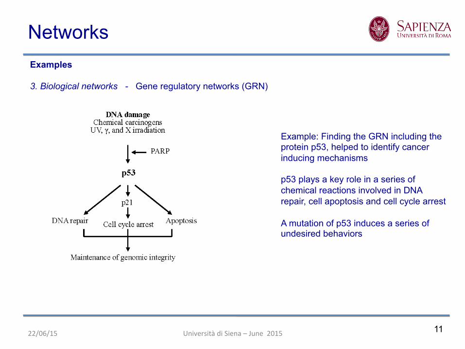
Examples 3. Biological networks - Gene regulatory networks (GRN)

Networks

11

Example: Finding the GRN including the protein p53, helped to identify cancer inducing mechanisms p53 plays a key role in a series of chemical reactions involved in DNA repair, cell apoptosis and cell cycle arrest A mutation of p53 induces a series of undesired behaviors


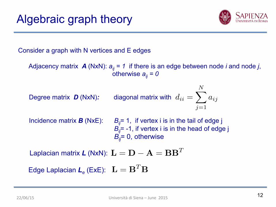
Consider a graph with N vertices and E edges Adjacency matrix A (NxN): aij = 1 if there is an edge between node i and node j, otherwise aij = 0 Degree matrix D (NxN): diagonal matrix with Incidence matrix B (NxE): Bij= 1, if vertex i is in the tail of edge j Bij= -1, if vertex i is in the head of edge j Bij= 0, otherwise Laplacian matrix L (NxN): Edge Laplacian Le (ExE):

Algebraic graph theory


L = D�A = BBT

L = BTB

dii =NX

j=1

aij

Example


13

1

2

3

5

4

L =

2

66664

2 �1 �1 0 0�1 3 �1 0 �1�1 �1 4 �1 �10 0 �1 2 �10 �1 �1 �1 3

3

77775

A =

2

66664

0 1 1 0 01 0 1 0 11 1 0 1 10 0 1 0 10 1 1 1 0

3

77775


Example


14

1

2

3

5

4

B =

2

66664

�1 �1 0 0 0 0 01 0 �1 �1 0 0 00 1 1 0 �1 �1 00 0 0 0 0 1 10 0 0 1 1 0 �1

3

77775

A =

2

66664

0 0 0 0 01 0 0 0 01 1 0 0 00 0 1 0 10 1 1 0 0

3

77775

Note: for a directed graph (digraph) L = D�A 6= BBT


Properties -  The total number of paths of length k between two nodes i and j is

-  The total number of loops of length k starting from node i is

-  The total number of loops of length k is

-  The number of triangles in a graph is

-  By construction, , hence is an eigenvector of associated to the zero eigenvalue

Given a vector defined over the vertices of a graph, the disagreement is

15

x

TLx =

X

u,v2E(xu � xv)

2


[Ak]ij

[Ak]ii

tr(Ak)

tr(A3)/6


L1 = 0 L1

x

Properties If G is a graph with c connected components rank (B) = N – c Sketch of the proof: Let us look at the (left) null space of B zT B = 0 if (u,v) is an edge of the graph zu – zv = 0 z is constant over each connected component How many independent z ? c Null space of B = c Equivalently, If G is a graph with c connected components rank (L) = N – c

16



Properties Let us denote by the eigenvalues of L -  By construction, the minimum eigenvalue of L is

-  The eigenvector associated to is composed of all ones

-  The multiplicity of equals the number of connected components

17

�1 �2 . . . �N

�1 = 0

�1 = 0

�1 = 0



Conductance Let be a subset of the vertex set V denotes the boundary of S, i.e. the set of edges with one end in S and the other end outside S Conductance: with Theorem: = second smallest eigenvalue of L measures graph connectivity

18

@S

S

� := minS

|@S||S|

|S| |V |/2

� � �2

2

�2



Eigen-decomposition of From Rayleigh-Ritz theorem

19



�min

(L) x

T

Lx

x

T

x

�max

(L)

u1 = argminx

x

TLx

x

Tx

ui = argminx

x

TLx

x

Tx

uTi uj = 0, j = 1, . . . , i� 1

subject to

ku1k = 1

kuik = 1

subject to

L

20

u2 u3

−1 −0.5 0 0.5 1 1.5−1

−0.5

0

0.5

1

1.5

2

−1 −0.5 0 0.5 1 1.5−1

−0.5

0

0.5

1

1.5

2

Examples of eigenvectors



Graph features Diameter: maximal distance (number of hops along the geodesic path) between any pair of nodes Denoting with the average degree in a random graph If the graph is composed of isolated trees If a giant cluster appears If the graph is totally connected and the diameter is concentrated around

Graph features


The clustering coefficient Ci for a vertex vi is given by the proportion of links between the vertices within its neighborhood divided by the max number of links that could possibly exist between them The clustering coefficient for the whole system is the average of the clustering coefficients:

22

- Clustering coefficient

Graph features


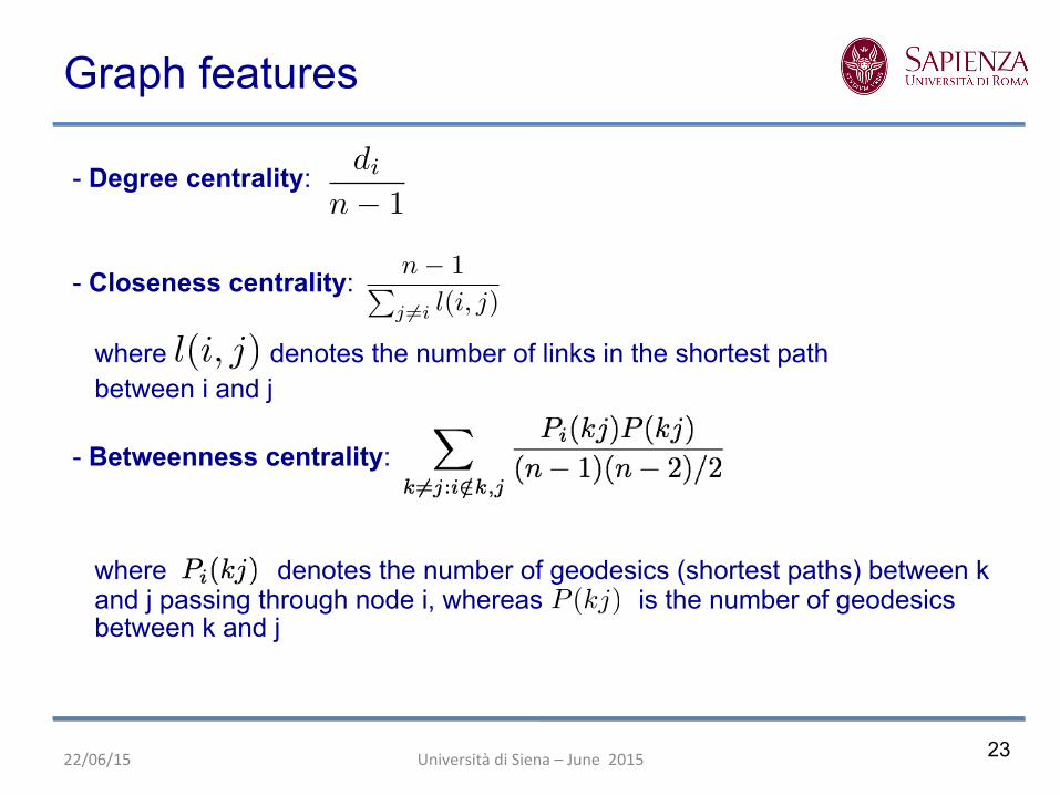
- Degree centrality: - Closeness centrality: where denotes the number of links in the shortest path between i and j

di

n� 1

n� 1�j �=i l(i, j)

l(i, j)

23

- Betweenness centrality: where denotes the number of geodesics (shortest paths) between k and j passing through node i, whereas is the number of geodesics between k and j

P (kj)

Graph features


Betweenness centrality – Example: fifteenth century Florence

BC(Medici) = 0.522 BC(Strozzi) = 0.103 BC(Guadagni) = 0.255

24

Graph features


Eigenvector centrality Idea: Importance of a vertex in a network increases by having connections to other vertices that are themselves important

The solution is given by the eigenvector associated to the largest eigenvalue of

25

Graph features


xi = ↵

NX

j=1

Aijxj x = ↵Ax

A

Erdos-Renyii Each node is connected with to each of the other nodes with probability The presence of links are statistically independent event The degree distribution is then mean degree: ; standard deviation: If the average of nodes s steps away from a random node is , the average number of steps necessary to reach any node is diameter:

Random graph models


pn� 1

pk =

✓n� 1k

◆pk(1� p)n�1�k

(n� 1)pp(n� 1)p(1� p)

cs

D ⇡ lnn

ln c

Erdos-Renyii Giant component (asymptotic behavior) Let us denote by u the fraction of nodes not belonging to a giant component For a vertex i not to belong to the giant component it must not be connected to the giant component via any other vertex For every other vertex j in the graph, either (a) i is not connected to j by an edge, or (b) i is connected to j but j is itself not a member of the giant component The total probability of not being connected to the giant component via vertex j is 1 − p + pu

Random graph models


u = (1� p� pu)n�1

Erdos-Renyii Giant component (asymptotic behavior) The fraction S of nodes in the giant component satisfies where

Random graph models

Note: transition phase


S = 1� e�cS

c = (n� 1)p

0 0.5 1 1.5 2 2.5 3 3.5 40

0.1

0.2

0.3

0.4

0.5

0.6

0.7

0.8

0.9

1

Mean degree c

Size

of t

he g

iant

com

pone

nt S

Phase transition in random graphs

Random graph models


Random graphs often exhibit phase transition phenomena as many physical systems, like water-ice transition, magnetism, … Phase transitions are often regulated by small variations of a single parameter, e.g. average degree, …

Small world networks Motivation Purely random graphs exhibit a small average shortest path length (varying typically as the logarithm of the number of nodes) along with a small clustering coefficient However, many real-world networks have a small average shortest path length, but also a clustering coefficient significantly higher than expected by chance Milgram experiment (six degrees of separation) A small-world network is a graph with high clustering coefficient, where most nodes are not neighbors of each other, but they can be reached from every other by a small number of hops

Random graph models


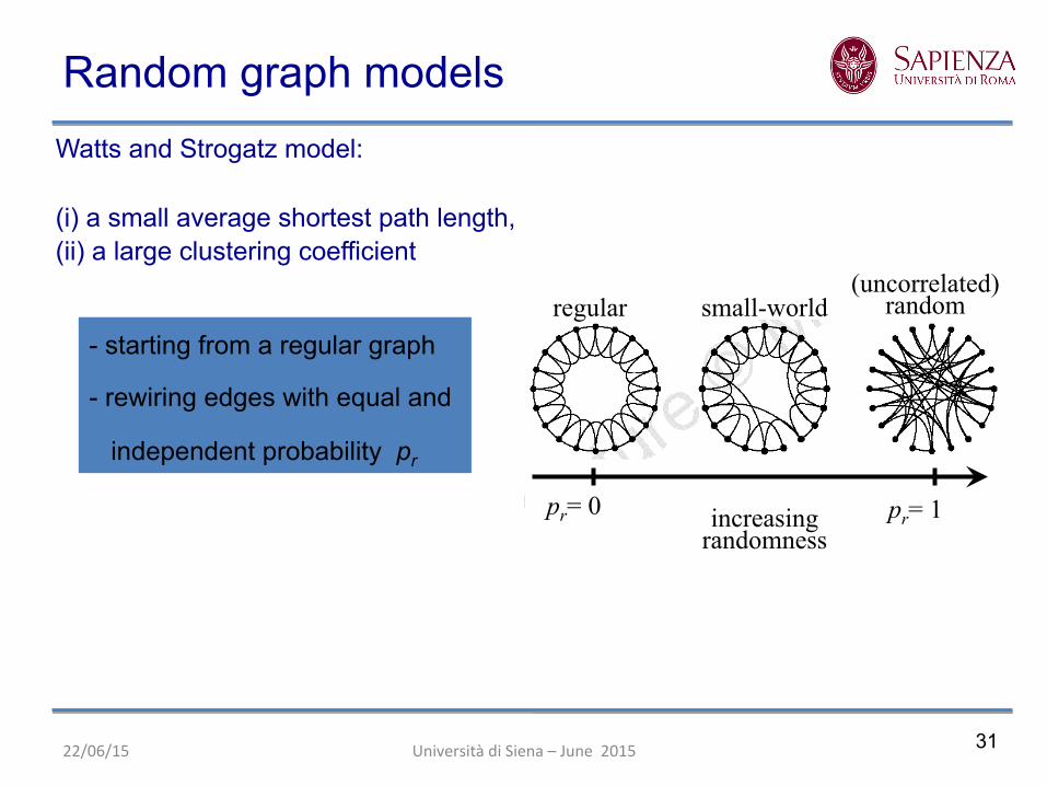
Watts and Strogatz model: (i) a small average shortest path length, (ii) a large clustering coefficient

-  starting from a regular graph

-  rewiring edges with equal and

independent probability pr

regular small-world (uncorrelated)

random

increasing randomness

pr= 0 pr= 1

31

Random graph models


for intermediate values of pr:

small-world behavior:

•  average clustering (C) high •  average distance (L) low

1 0.01

1

0.5

0 pr= 0

32

Watts and Strogatz model: (i) a small average shortest path length, (ii) a large clustering coefficient

Random graph models


33

Scale-free model In most real networks, the degree distribution follows a polynomial law decay, as opposed to exponential decay of purely random networks

scale-free networks

random networks

Scale-free networks exhibit polynomial decay Scale-free networks can be grown through a preferential attachment rule

Random graph models


34

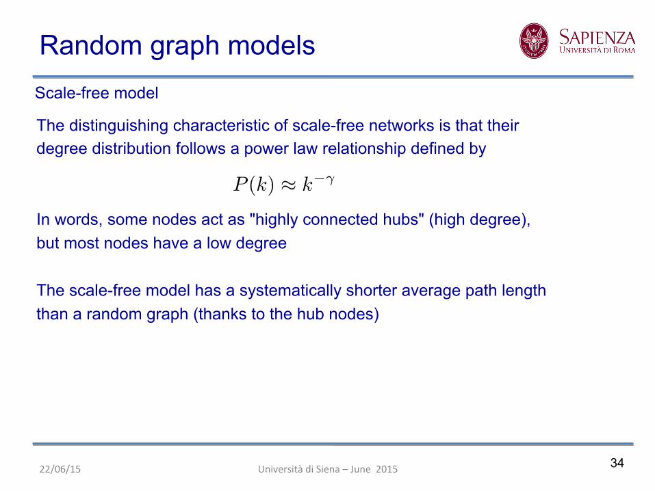
Scale-free model

Random graph models


The distinguishing characteristic of scale-free networks is that their degree distribution follows a power law relationship defined by In words, some nodes act as "highly connected hubs" (high degree), but most nodes have a low degree The scale-free model has a systematically shorter average path length than a random graph (thanks to the hub nodes)

P (k) ⇡ k��

35

Random graph models


Network building rules (dynamic) 1. The network begins with an initial network of m0 (>1) nodes 2.  Growth: New nodes are added to the network one at a time

3.  Preferential attachment: Each new node is connected to m of the existing nodes with a probability proportional to the number of links that the existing node already has. Formally, the probability that the new node is connected to node i is

where is the degree of node i (rich get richer)

36

Random graph models


Random geometric graphs A random geometric graph is a random undirected graph drawn on a bounded region It is generated by:

1. Placing vertices at random uniformly and independently on the region

2. Connecting two vertices, u, v if and only if the distance between them is smaller than a threshold r

37

Random graph models


Def.: A graph is said to be k–connected (k=1,2,3,...) if for each node pair there exist at least k mutually independent paths connecting them

Equivalently, a graph is k–connected if and only if no set of (k−1)nodes exists whose removal would disconnect the graph The maximum value of k for which a connected graph is k–connected is the connectivity κ of G. It is the smallest number of nodes whose failure would disconnect G As r0 increases, the resulting graph becomes k–connected at the moment it achieves a minimum degree dmin equal to k

Random geometric graphs

38

Random graph models


Random geometric graphs

Thm (Gupta & Kumar): Given a graph G(n, rn), with the graph is connected with probability one as n goes to infinity if and only if Example:

rn =

rlog n+ cn

⇡n

limn!1

cn = 1

rn =

r2 log n

⇡n

39

Operations on graphs

Graph partitioning Given a graph, split in two complementary subsets S and Sc, let us associate different labels to nodes belonging to different subsets:

si= 1, if i belongs to S, si= -‐1, if i belongs to Sc

Note

0.5 si sj = 0, if i and j belong to the same set, 0.5 si sj = 1, if i and j belong to different sets

DefiniFon: Cut size = Problem: Split a graph in two subsets in such a way that the cut size is minimum

R =1

4

X

i

X

j

Aij (1� sisj)


40


Graph partitioning Cut size can be rewri\en as Constraints: -‐ number of nodes / cluster -‐ bounded norm Problem formulaFon:


R =1

4sTLs

s = argmin sTLs

NX

i=1

si = n1 � n2

si 2 {�1, 1}subject to

This is a combinatorial problem

41


Graph partitioning Relaxed problem:


s = argmin sTLs

NX

i=1

si = n1 � n2

subject to

Lagrangian:

NX

i=1

s2i = N

L(s;�, µ) =NX

k=1

NX

j=1

Ljksjsk + �

0

@N �NX

j=1

s2j

1

A+ 2µ

0

@n1 � n2 �NX

j=1

sj

1

A

Ls = � s+ µ1

Se_ng the gradient to zero, we get

42


Graph partitioning Relaxed problem: MulFplying from the le` side by , we get Introducing the vector we get is then an eigenvector of The cut size can be rewri\en as


x := s+µ

�1 = s+

n2 � n1

N1

µ =n2 � n1

N�sT

Lx = �x

x

L

R =n1n2

N�

43


Graph partitioning Relaxed problem: is then the eigenvector associated to the second smallest eigenvalue of : The (real) soluFon is then The closest binary soluFon is obtained by maximizing the scalar product The opFmal is achieved by assigning to the verFces with the largest and to the other verFces


Lx

u2

sR = x+n1 � n2

N1

sT sR

sxi + (n1 � n2)/N

si = +1 n1

si = �1

44


Graph partitioning Example


−1 −0.5 0 0.5 1 1.50

0.2

0.4

0.6

0.8

1

1.2

1.4

1.6

−0.06

−0.04

−0.02

0

0.02

0.04

0.06

45


Graph partitioning


−1 −0.5 0 0.5 1 1.5−1

−0.5

0

0.5

1

1.5

2

−0.06

−0.04

−0.02

0

0.02

0.04

0.06

−1 −0.5 0 0.5 1 1.5−1

−0.5

0

0.5

1

1.5

2

−0.06

−0.04

−0.02

0

0.02

0.04

0.06

0.08

u2 u3

References

46

1.  M. Newman, Networks: An IntroducFon, Oxford Univ. Press, 2010

2.  C. Godsil, and G. Royle, Algebraic Graph Theory , Springer, New York, 2001

3.  M. Mesbahi, M. Egerstedt, Graph TheoreFc Methods in MulFagent Networks, Princeton Univ. Press, 2010

4.  R. Albert and A.-‐L. Barabasi, “StaFsFcal mechanics of complex networks," Reviews of Modern Physics, 74(1), pp.47-‐97, 2002.


signal processing over graphs: distributed optimization...

Documents