signal-to-noise ratio of the bispectral analysis of ... · the signal-to-noise ratio of the...

Vol. 5, No. 9/September 1988/J. Opt. Soc. Am. A 1477

Signal-to-noise ratio of the bispectral analysis of speckleinterferometry

Tadashi Nakajima

Division of Physics, Mathematics, and Astronomy, California Institute of Technology, Pasadena, California 91125

Received February 8, 1988; accepted April 26, i988

Monte Carlo simulations of an atmospheric phase screen, based on a Kolmogorov spectrum of phase fluctuations,were performed. Speckle patterns produced from the phase screens were used to derive statistical properties ofpower spectra and bispectra of speckle interferograms. We present the bispectral modulation transfer function andits signal-to-noise ratio at high light levels. The results confirm the validity of a heuristic treatment based on aninterferometric picture of speckle pattern formation in deriving the attenuation factor and the signal-to-noise ratioof the bispectral modulation transfer function in the mid-spatial-frequency range. The derived modulationtransfer function is also interpreted in terms of the signal-to-noise ratio at low light levels. A general expression ofthe signal-to-noise ratio of the bispectrum is derived as a function of the transfer functions of the telescope, thenumber of speckles, and the mean photon counts in the mid-spatial-frequency range.

1. INTRODUCTION

Speckle interferometry' was first extended to full imagingwith phase by Knox and Thompson. 2 A more powerfulimaging technique, based the use of closure phase, 3 wasdeveloped in radio astronomy. Independently, for opticalwavelengths, a method to extract closure-phase informationfrom speckle observations by means of the bispectrum wasdeveloped by the Erlangen group.4 So far, the method,called bispectral analysis, has been successful in recovering a10th-magnitude multiple stellar system.5 However, the po-tential and the limitations of the method have not yet beeninvestigated fully both in sensitivity and resolution. It isimportant to quantify the behavior of the signal-to-noiseratio (SNR) of the bispectrum, which depends on both thespatial frequency and the light level.

The analysis of the SNR of the bispectral analysis is paral-lel to that of the power spectrum analysis and comprises twostages. First the modulation transfer functions (MTF's)that describe the combined effect of the telescope and theatmospheric disturbance are obtained by treating an incom-ing light as a wave and treating a speckle interferogram as anintensity distribution. By taking the influence of photonnoise into account, the SNR of the bispectrum at arbitrarylight levels is determined as a function of the classical MTF'sand the mean photon counts.

In most discussions of the SNR in the literature on speckleinterferometry, MTF's are derived in the mid-spatial-fre-quency range, based on the heuristic interferometric view(HIV) of the image-forming process.6 From this point ofview, a speckle pattern is regarded as a random interferencepattern produced by a partially coherent incident wave.The validity of this heuristic treatment is known empiricallyin the case of the power-spectrum analysis. The effect ofthe atmospheric disturbance is included in only one parame-ter, the coherence length. The existence of the steep Kol-mogorov spectrum in phase fluctuations suggests that theremay be some important effects that are not predicted by thissimple approach. A more thorough derivation of the power-

spectrum MTF, based on the phase structure function of theKolmogorov theory, was derived by Korff,'7 who used a semi-analytical approach that took the atmospheric turbulenceproperly into account. The derivation of the power-spec-trum MTF is close to the limit of what can be done analyti-cally. In order to obtain higher-order MTF's, such as thebispectral MTF, that take the Kolmogorov theory into ac-count, it is necessary to resort to Monte Carlo simulations.This method enables us to test the predictions of the HIV ofthe bispectral analysis,8 -10 and it is shown here that thosepredictions can be used as a guide to the correct first-orderresults. Predictions of the HIV are summarized in Appen-dix A of this paper.

The modeling of the photodetection process, based on therules of conditional statistics, and its application to the pow-er-spectrum analysis were given by Goodman andBelsher,11-"3 who formulated an unbiased estimator of theclassical power spectrum from an ensemble of photon-noise-limited images. They also obtained an expression for theSNR of the power spectrum in terms of the classical MTFand the mean photon counts. Their analysis is applicable tonon-photon-counting detection. In other words, they treat-ed a case in which average photon counts per image weremeasurable but neither the positions of the individual pho-tons nor the total photon counts of individual images wereknown. Dainty and Greenaway14 applied the approach ofGoodman and Belsher"1-"3 to photon-counting detectionand pointed out that an unbiased estimator of the powerspectrum is given in the same manner as in the case of non-photon-counting detection but the expression for the SNR isdifferent. Since the photon-noise bias can be removed ineach frame, the variance of the power spectrum does notinclude terms originating from the fluctuations of the bias.

Wirnitzer'5 gave an unbiased estimator of the classicalbispectrum, applying the method of Goodman andBelsherll-13 to the bispectral analysis for photon-countingdetection. Wirnitzer also obtained the SNR in the high-and low-light limits by evaluating the corresponding leadingterms in the power of photon counts. This was the first

0740-3232/88/091477-15$02.00 © 1988 Optical Society of America

Tadashi Nakajima

1478 J. Opt. Soc. Am. A/Vol. 5, No. 9/September 1988 Tadashi Nakajima

realistic attempt to estimate the limiting magnitude of thebispectral analysis. However, as was first pointed out byKarbelkar and Nityananda,9 the classical bispectral MTFadopted by Wirnitzer and the SNR in the high-light limit donot agree with those derived from the treatment based onthe HIV.

Monte Carlo simulations of an atmospheric phase screen,based on the Kolmogorov spectrum derived by Tatarskii,' 6 ,17

were made in order to study statistical properties of thebispectral MTF at high light levels. The algorithm and thecomputation are described in Sections 2 and 3, respectively.The results of the simulations for a 2-m telescope are pre-sented in Section 4. The results are compared with thoseobtained by using the interferometric view in Section 5.The MTF obtained by the simulations is reinterpreted toyield the SNR at low light levels in Section 6. In Section 7the discussion of the SNR is generalized to arbitrary lightlevels and arbitrary telescope sizes by modeling of the photo-detection process and the approximate MTF's in the mid-frequency range. Finally, in Section 8 the SNR in the recov-ered map is considered. An estimate of the practical limit-ing magnitude is discussed along with the limitation inresolution.

2. ALGORITHM

The simulations are based on the Kolmogorov theory ofturbulence and refractive-index fluctuation' 6-'8 and on re-cent observations of the altitude dependence of the refrac-tive-index structure constant Cn2 (e.g., the La Silla SeeingCampaign19' 20). The Kolmogorov theory provides mathe-matical expressions of the atmospheric disturbance on alight-wave propagation as two-dimensional spectral densi-ties of phase fluctuation and amplitude fluctuation and thecross spectral density of the two. On the other hand, recentobservations indicate that most of the turbulence is pro-duced at the boundary layer and that the high-altitude tur-bulence contributes a relatively small fraction of the overallseeing degradation. We therefore assume that the majordisturbance appears as phase fluctuations in the near-fieldlimit and that the amplitude fluctuation (scintillation) andthe cross correlation of the phase and the amplitude fluctua-tions are negligible to first order.

In the near-field limit, the spectral density of the phasefluctuation at the aperture plane of a telescope is given by

FS(Kr) = 0.03321rk2[J Cfl2(L)dL]Kr-11/3, (2.1)

where Kr = (Kx2 + KY

2)1/

2 is the two-dimensional radial spatialfrequency, k is the wave number, and f C,2(L)dL is theintegrated structure constant of the refractive-index fluctu-ation over the optical path through a turbulent medium.

Since the spectral density constrains the frequency-de-pendent variance of the fluctuation but not the probabilitydistribution, we further assume a Gaussian probability dis-tribution with zero mean. In what follows, 4(x) denotes thephase at the aperture plane of a telescope and is a realfunction of x, and @(K) denotes its Fourier transform, whichis a conjugate-symnmnetric-complex function of K. At eachpoint over one half of the K space, @(K), a complex randomnumber whose modulus is a Gaussian random number with avariance of FS(Kr)AK and whose phase is a uniform random

number between 0 and 27r, is generated. AK denotes an areain K space equaling (27/lmax)2, where 1max is the size of thesquare phase screen. A conjugate-symmetric-to-real Fouri-er transform from K to x space then creates a monochromaticphase screen b(x) at A = 27r/k.

An idealized telescope is simulated simply by a circularaperture on the phase screen. At each point of the apertureplane, the complex amplitude T(x) = exp[ib(x)] is calculat-ed. Another Fourier transform simulates the light-wavepropagation from the aperture plane to the image plane, andfrom the squared modulus of the Fourier transform of I(x),a monochromatic speckle pattern, ['I'(s) 12, is obtained, wheres denotes the coordinate on the image plane. Since thephase fluctuations are simply proportional to the wave num-ber k, the finite-bandwidth effect is taken into account byaveraging over monochromatic speckle patterns at equallyspaced wave numbers covering the bandpass. Thus, fromone evaluation of '(x), multiple IjII(s)I2 are generated andaveraged to produce one speckle interferogram I(s). If Tay-lor's hypothesis of frozen-in turbulence2' and a uniformtranslation by a constant wind velocity are assumed, a con-tinuous observation can be simulated by considering a seriesof apertures displaced by a distance that is typically thecoherence length, r,.

In the data reduction, many short-exposure frames areprocessed to derived statistics. The Fourier transform Ij(u)of the speckle interferogram of the jth frame Ij(s) is taken toform the bispectrum,

B3j")(u,, u2) = 1j(u1)Ij(u2 ) 1j(-U1 '-U"9 (2.2)

where u denotes the spatial frequency on the image plane.For n frames, both the sum of bispectra,

n

E' B[j(3)(Ul, U2),j=1

and the sum of square moduli,

jf3jl)(U,, U2)12,

(2.3)

(2.4)

are calculated. The unbiased estimator of the ensemble-average bispectrum is

n

1 B3j (3)(Ul, U2)

0 (N uP U2)) = j1, (2.5)n

where ( ) indicates an ensemble average. Likewise the un-biased estimator of the variance of the bispectrum per frameis

n

> IA'j(3)(u, U2) 12-n1(B3(U, U2))12

u2[B3(u3 , U 2)I = j1

(2.6)

In the case of the bispectral MTF, the mean value is real,3since the atmospheric disturbance is statistically isotropicand the ideal telescope is static and symmetric. After aver-

n

j=1


aging over enough samples, the SNR of the MTF per frameis defined as

N[B~(u, u2 )] =Re[(B(3)(ul, u2))] (2.7)

77

D

Henceforth a SNR is taken to mean a SNR per frameunless specified otherwise. The SNR in the recovered mapis discussed in Section 8.

3. COMPUTATION

The simulations were made at a wavelength X = 0.55 ,gm witha fractional bandwidth of 0.1. At this wavelength, the inte-grated structure constant of the refractive-index fluctua-tion,

J C"2 (L)dL = 5 X I0O-3 ml/'3 , (3-1)

was adopted corresponding to 1-arcsec seeing. This is ap-proximately Roddier's value.2 2 It was found experimentallythat five monochromatic speckle interferograms producedat equally spaced wave numbers within the bandpass wereenough to obtain a reasonable averaged speckle interfero-gram.

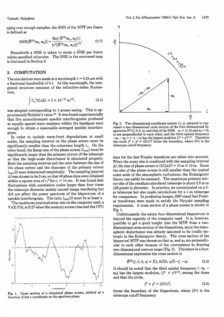
In order to include wave-front degradations at smallscales, the sampling interval on the phase screen must besignificantly smaller than the coherence length r,. On theother hand, the linear size of the phase screen (lma,) must besignificantly larger than the primary mirror of the telescopeso that the large-scale disturbance is simulated properly.Both the sampling interval and the ratio between the size ofthe phase screen and the diameter of the primary mirrorlmax/D were determined empirically. The sampling intervalAl was chosen to be 2 cm, so that 49 phase data were obtainedwithin a square area of r,2 for r, = 14 cm. It was found thatfluctuations with correlation scales larger than four timesthe telescope diameter mainly caused image wandering butdid not affect the power spectrum of the bispectrum of aspeckle interferogram. The ratio lmax/D must be at least 4.

The maximum practical array size on the computer used, aVAX/750, is 5122 when the memory access time and the CPU

CD

Fig. 2. Two-dimensional coordinate system (D t), adopted to rep-resent a two-dimensional cross section of the four-dimensional bi-spectrum b(3)(t, 0,0, ii), and that of the SNR. uj = (D, 0) and U2 = (0,w) are perpendicular to each other, and the third spatial frequency-Ul-U2 = (-i,-n) has the largest modulus (r + ,12)1/2. Thereforethe circle t2 + r7

2 = (D/X)2 forms the boundary, where D/X is thetelescope-cutoff frequency.

time for the fast Fourier transform are taken into account.When the array size is combined with the sampling intervalAl, the size of phase screen is (512Al) 2 10 m X 10 m. Since

the size of the phase screen is still smaller than the typicalouter scale of the atmospheric turbulence, the Kolmogorovtheory can safely be assumed. The maximum primary mir-ror size of the resultant simulated telescope is about 2.5 m or128 pixels in diameter. In practice, we concentrated on a 2-m telescope but also made calculations for a 1-m telescopefor comparison. In producing images, 2562 -sized fast Fouri-er transforms were made to satisfy the Nyquist samplingrequirement. A cross section of a phase screen is shown inFig. 1.

Unfortunately the entire four-dimensional bispectrum isbeyond the capacity of the computer used. It is, however,possible to get a good insight into the MTF from a two-dimensional cross section of the bispectrum, since the atmo-spheric disturbance was already assumed to be locally iso-tropic in the Kolmogorov theory. The cross section of thebispectral MTF was chosen so that ul and u2 are perpendic-ular to each other because of the convenience in drawingtwo-dimensional contour maps (Fig. 2). Therefore in a four-dimensional expression the cross section is

13f)(j; 0, 0, Oq) = I(, 0)I(0, )I(- n,-). (3.2)

It should be noted that the third spatial frequency (-ul -u2) has the largest modulus, (?e + r/2)1/2, among the threeand that the circle,

e2 + 7 2 = (D/X)2, (3.3)

forms the boundary of the bispectrum, where D/X is thetelescope cutoff frequency.

coordiate(r)

Fig. 1. Cross section of a simulated phase screen, plotted as afunction of the x coordinate on the aperture plane.

Tadashi Nakajima

1480 J. Opt. Soc. Am. A/Vol. 5, No. 9/September 1988

4. RESULTS OF THE SIMULATIONS

The results of the computations are the normalized bispec-tral MTF's, defined as

(B,(3)(0, 0)) (4.1)

Since fluctuations in the total intensity I(0) = f I(x)dx arenot considered,

(fr')(O, 0)) = A(0)M = const.,

and then

(b')(ul, U2)) = (T(u,)T(u2)T(-u1 -U2))

(4.2)

(4.3)

where i(u) = 7(u)/l(0). For the same reason, the SNR in thenormalized bispectral MTF is

SNR[6(')(uj, u2 )] = SNR[f(3)(u,, U2)]- (4.4)

The r and -q axes on the t-77 plane correspond to thenormalized power-spectrum MTF:

(5(3)(D, 0, 0, 0)) = (T(r, 0)i(0, 0)T(-, 0))

= (T(D, 0)1T(¢, 0)*)

= (JT(I, 0)12), (4.5)

and, similarly,

(&(6 )(0, 0, 0, n)) = ( I(o 77)12). (4.6)

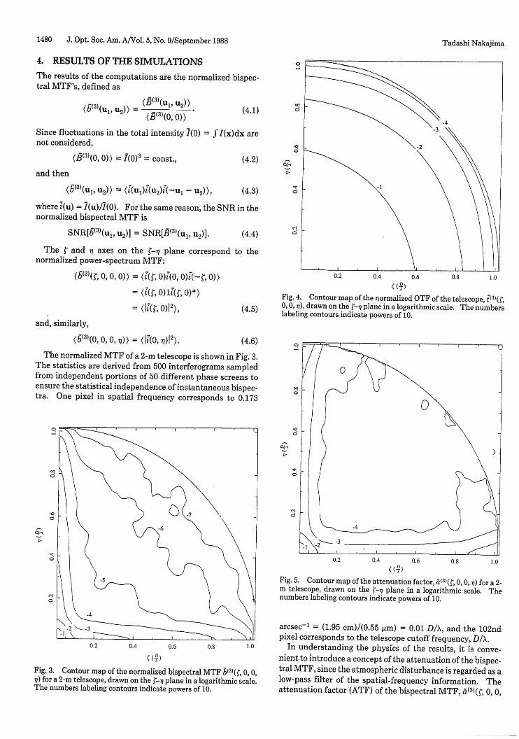
The normalized MTF of a 2-m telescope is shown in Fig. 3.The statistics are derived from 500 interferograms sampledfrom independent portions of 50 different phase screens toensure the statistical independence of instantaneous bispec-tra. One pixel in spatial frequency corresponds to 0.173

0

6o

6

6i

0.2 0.4 0.6 0.8 1.0( t A)

Fig. 4. Contour map of the normalized OTF of the telescope, t(3)(¢,0, 0, i7), drawn on the {-17 plane in a logarithmic scale. The numberslabeling contours indicate powers of 10.

9

6o

6O1k

61

6o

0

ci6o

Fig. 3. Contoui1) for a 2-m telesThe numbers lal

0.2 0.4 0.6 0.8 1.0( (DA)

Fig. 5. Contour map of the attenuation factor, &(3)(t, 0, 0, 7) for a 2-m telescope, drawn on the A-,1 plane in a logarithmic scale. Thenumbers labeling contours indicate powers of 10.

3 - \)arcsec-1 = (1.95 cm)/(0.55 ktm) = 0.01 D/X, and the 102ndI I _t_-x > 1)pixel corresponds to the telescope cutoff frequency, D/X.

0.2 0.4 0.6 0.8 1.0 In understanding the physics of the results, it is conve-( ( i)) nient to introduce a concept of the attenuation of the bispec-

r map of the normalized bispectral MTF b(3)(D, 0, 0 tral MTF, since the atmospheric disturbance is regarded as acope, drawn on the {-71 plane in a logarithmic scale. low-pass filter of the spatial-frequency information. The)eling contours indicate powers of 10. attenuation factor (ATF) of the bispectral MTF, &(3)(t, 0, 0,

9

coTo

0

Tadashi Nakajima


0) is defined along with the optical transfer function (OTF)of the telescope, j(3)(D, 0, 0, 7), as

(a(3)(~' 0, 0, a)) = (b(3( 0, 0, 1))F'3)(' 0, , ,)

(4.7)

where 1(3)(¢, 0, 0, 77) is static and real. The OTF is thenormalized bispectrum of the Airy pattern and thus is thenormalized MTF under the coherent illumination. It couldalso be interpreted as the relative weight of the frequencycomponents or the relative redundancy of the triangularbaselines (both closed and nonclosed) on the primary mirror.To avoid confusion, it should be noted that the attenuationis the combined effect of the atmosphere and the optics andthus that the ATF depends on the OTF even for a givenatmospheric condition. The OTF and the ATF are shown inFigs. 4 and 5, respectively. The OTF is a monotonicallydecreasing function of r and 7. It is fairly flat at (r + 772)1/2

' 0.5 D/X and then falls more steeply at higher frequencies.The ATF, and thus the MTF, behave in a more complicat-

ed manner. The SNR of the classical MTF or the saturatedSNR at high light levels is shown in Fig. 6. The behavior ofthe SNR is quite similar to that of the ATF. Semiquantita-tively, the contour maps of the ATF and the SNR can beclassified into five distinct regions in spatial frequency asfollows.

A. Low-Frequency Region [(f2 + n72)1

/2 < 0.1 D/XA

The ATF is larger than 0.01 and the SNR is larger thanunity. The information of this region originates from theenvelopes of instantaneous interferograms. Even this low-frequency region has better information than a seeing diskobtained by a long time exposure, since the effect of imagewandering is removed.

9

Iq

6

'0

Cld

6E

0 0.2 0.4 0.6 0.8 1.0

Radial Spatial Frequency Jul (A)

Fig. 7. Power-spectrum atmospheric transfer function l(u)12,plotted as a function of the modulus of the radial spatial frequencyul.

B. On-Axis Region (D = 0, 77 = 0)The power-spectrum ATF is plotted as a function of radialfrequency in Fig. 7, since it is statistically isotropic. TheATF falls off steeply at low frequencies (<0.1 D/X) and thenlevels between 0.1 D/X and 0.8 D/X at around 4 X 10-3.Above 0.8 D/X, the ATF slowly rises up to 10-1 at D/X. Thisincrease in the ATF at high spatial frequencies is not fastenough to compensate for the steep fall of the OTF, and thepower-spectrum MTF monotonically falls off, as is shown onthe axes in Fig. 3. The SNR is larger than 0.8 up to D/X.

C. Near-Axis Region (D • 0.1 D/X, or i7 ' 0.1 D/X)The ATF falls off steeply to 10-4, and the SNR decreases to0.3 as the plot moves vertically saway from each axis. Thebispectral components are the combination of the low-fre-quency Fourier components and the power spectrum.Phases of the bispectral components in this region are effec-tively local phase differences of nearby Fourier components,which are used in the Knox-Thompson method. 2

D. Mid-Frequency Region [r, i1 > 0.1 D/X and (r2 + 772)1/2

< 0.8 D/XI

A large triangular plateau of the ATF with a mean value of 3

X 10-5 is evident in Fig. 5. In this region, the behavior of the0.06 CJ ( \MTF is determined mainly by that of the OTF. The MTF

falls from 10-4 to 10-6. The SNR is between 0.1 and 0.2.

0.1 EJ E. High-Frequency Region [r2 + X72 (D/X)2 J

The diffraction-limited information lies in this region. Be-cause of the steep fall of the OTF, the MTF is very small

0 2 (<10-7). The SNR is smaller than 0.1.

-0.

0.6 I _ = 1 5. COMPARISON WITH THE HEURISTIC

0.2 0.4 0.6 0.8 1.0 INTERFEROMETRIC VIEW((A)

Fig. 6. Contour map of the SNR of the bispectral MTF SNR[b(3 )(D,0, 0, 7)] for a single frame obtained with a 2-m telescope, drawn onthe t-77 plane. This map shows the saturated SNR at high lightlevels.

It is interesting to compare the results described in sectionfour with the predictions obtained by using the HIV of theimage-forming process. A brief description of this view isgiven in Appendix A, and a detailed discussion is found in

l I l l l l l l l I

. , . , . I . I

Tadashi Nakajima

1482 J. Opt. Soc. Am. A/Vol. 5, No. 9/September 1988 Tadashi Nakajima

Ref. 10. The HIV predicts that the power-spectrum ATF isapproximated by n,-1 = (rI/D) 2, where n, is the number ofspeckles, and that the SNR of the power spectrum is unity inthe mid-frequency range. It also estimates that the bispec-tral ATF in the mid-frequency range is about n,- 2 = (r,/D)4

and that the SNR is given by n,-1/2 = r/D. The bispectralATF and its SNR are therefore related by

(5.1)

Thus the similarity of the contour maps of the ATF and theSNR, which are plotted in logarithmic scale in Figs. 5 and 6,is naturally explained by the HIV. For r, = 14 cm and D = 2m, n, = 204. The flat portion of the simulated power-spectrum ATF between 0.2 D/I and 0.8 D/A is 4 X 10-3 onaverage, whereas the value predicted by the HIV is 5 X 10-3.

The SNR of the power spectrum lies between 0.6 and 0.8 andis approximately unity. At the mid-frequency region, thesimulated bispectral ATF has an average value of 3 X 10-5,whereas the value predicted by using the HIV is 2 X 10-5.We consider this agreement good.

The simulations were also made for a 1-m-diameter tele-scope. For a telescope of this size the midfrequency of thepower spectrum ranges from 0.3 D/A to 0.6 D/A, and thesimulated power-spectrum ATF is 3 X 10-2, whereas thepredicted value is 2 X 10-2. The SNR of the power spec-trum is between 0.7 and 1.0. The simulated bispectral ATFat the mid frequency is 2 X 10-3 in average, which is some-what larger than the predicted value, 4 X 10-4. The agree-ment is not so good as for a 2-m telescope.

The rise of the power-spectrum ATF at the high-frequen-cy region ('0.8 D/X for D = 2 m) can be interpreted qualita-tively by the HIV. At the high-frequency region, the redun-dancy (or OTF) of the baselines is so small and the identicalbaselines are so localized on the primary mirror that thephasors of those baselines are correlated and increase theATF. The approximate validity of the HIV of the image-forming process is confirmed by the simulations. The simu-lations also clarified the boundaries of the mid frequency forgiven apertures. Because of the higher redundancy and thewider mid-frequency range, the predictions made by usingthe HIV work better for larger telescopes.

9

0

'0

41-c

6t

ci

6

0.2 0.4 0.6 0.8 1.0

Fig. 8. Contour map of the SNR for a V = 12.3 magnitude starobtained with a 2-m telescope after integrating 104 frames, assuminga 10% observing efficiency, a 10% fractional bandwidth and a 10-msec integration time. These brightness and observing efficienciescorrespond to 1 photon per speckle.

9

6q

'0

6D~

lH

0

6. SIGNAL-TO-NOISE RATIO AT LOW LIGHTLEVELS

At low light levels, the SNR per frame of an unbiased estima-tor of the classical bispectral MTF is approximated by

(6(3)(ul, u2)) x p73/2'

Cl

(6.1)

where N is the average photon count per frame.I5 Thereforethe contour map of (b(3)(ul, u2)) can be converted immedi-ately to that of the SNR.

Figure 8 shows the SNR of a V = 12.3 magnitude star witha 2-m telescope after integrating 104 frames; this magnitudecorresponds to one photon per speckle in a 10% fractionalbandwidth, with 10% efficiency of the observing system anda 10-msec integration time. The SNR = 3 contour reachesthe diffraction limit on the axes but stays near the axis as or77 increases. The slope of the contours is the steepest diago-nally. Figure 9 shows SNR = 3 contours according to thebrightness of the sources. At 9.0 magnitudes the bispectralanalysis is diffraction limited in the sense of a 3a detection,

Fig. 9.levels.Fig. 8.

0.2 0.4 0.6 0.8 1.0

((A)

Behavior of 3a contours, plotted according to the lightMagnitudes are calculated for the same conditions as for

whereas at 13.9 magnitudes even the power-spectrum analy-sis is not necessarily diffraction limited, and the region ofhigh SNR is strictly near the axes.

The contour maps immediately show that the power spec-trum in general has a better SNR than the bispectrum. Theclosure-phase information obtained by near-axis bispectral

(&"'(Ull U2)) - jSNR[P)(uj, U2)114.


components is effectively the local phase differences ofneighboring Fourier components. For a simple source suchas a multiple stellar system, the autocorrelation functioncontains most of the source structure. The behavior of thephase in Fourier space is fairly regular, and thus the localphase differences are enough to recover a full image. Hof-mann and Weigelt5 used only the 5% of the bispectrum nearthe axes with the highest SNR for their image recovery.The result of the simulations is consistent with their obser-vations. The wide mid-frequency range contains global clo-sure-phase information with lower quality. For a compli-cated source, mid-frequency components may be crucial inrecovering a full image. Intensive computations are re-quired for utilization of the full bispectrum.

7. SIGNAL-TO-NOISE RATIO AT ARBITRARYLIGHT LEVELS

In the simulations, the incoming light is treated as a wave.Thus, from the point of view of photon detection, a limitingcase with an infinite number of photons is considered. Inthis section, by using the modeling of the photodetectionprocess by Goodman and Belsher"l-1 3' 23 and following thetreatment of the influence of photon noise on the bispectralanalysis by Wirnitzer,15 the derivation of an unbiased esti-mator of the classical bispectrum is reviewed, and then anexpression for the SNR of the bispectral MTF is obtained asa function of the mean photon count, the OTF's of tele-scopes, and the number of speckles.

We consider a speckle observation by using a photon-counting detector that records the positions of individualphotons detected on the image plane. The raw intensity ofthe jth frame is given as

Nj

Dj(x) = E(x - Xk), (7.1)k=1

where Xk is the position of the kth photon and Nj is the totalnumber of photons. The Fourier transform of Eq. (7.1) is

Nj

Dj(u) = J (x - xk)exp(iux)dx

Nj

= Z exp(iuxk). (7.2)k=1

The bispectrum of the raw data is given as

5j(3 )(u1, u2) = Dj(ul)Dj(u 2)Dj(-U 1 - U2)

Nj Nj Nj

= I I I expfi[ul(xk - Xm) + U2(XI - Xm)]1.k=1 1=1 m=1

(7.3)

The expected value of .1 ( 3)(ul, u2) is evaluated over theconditional statistics of XkS, Nj, and the rate function Xj(x),which is proportional to the classical intensity, Ij(x). For agiven Nj and Xj(x), the event locations x are independentrandom variables with a common probability-density func-tion,

p(X) = Xj(x) Ij(X))

J Xj(x)dx | Ij(x)dx

The characteristic function of pj(x) equals the normalizedFourier transform of the classical intensity distribution

pj(u) = J pj(x)exp(iux)dx

| Ij(x)exp(iux)dx

J Ij(x)dx

Ij(u)

ii()..Dj(3)(u1 , u2) is averaged first over the conditional statistics ofXk, x1 , and xm and then over Nj and Xj(x). The starting pointis the evaluation of

Eklm[.j(3)(Ul, u2 )J

Nj Nj Nj

= Eklm Z EX expli[u(xk -Xm) + U2(X1 Xm)]1)|k=1 1=11m=1

Nj Nj N.

= EE Ek~m (expli[Ul(Xk Xh) + U2(X1 Xm)]),k=l 1=1 m=l

(7.6)

where Ekl00 stands for an average over Xk, xi, and Xm. TheNj 3 terms are classified as follows:

(1) For k = I = m and Nj terms,

Eklm(l) = pj(Xk)dxk = 1

(2) For k 0 1 = m and Nj(Nj - 1) terms,

Eklmjexp[iul(Xk - k)]j}

= J J exp[iul(xk - x)] pj(xk)pj(xl)dXkdxl

= [JPj(Xk)exP(iulxk)dxk] [JPj(xl)exP(-iulxl)dXI]

= 'ij(Ulij-

= 1i7(ul)12 ,

where I7j(ui)12 is the normalized power spectrum.

(3) For k = m F 1 and Nj(Nj - 1) terms,

Eklmtexp[iul(xl - Xm)]} = I7(U2)12.

(4) For k = 1 5d m and Nj(Nj - 1) terms,

Eklmlexp[i(-ul - u2)(x - Xm)]I = 1T(/u1 - U2)12. (7.10)

(7.4)

(7.7)

(7.8)

(7.9)

Tadashi Nakajima

(7.5)


(5) For k , I m and Nj(Nj - 1)(Nj - 2) terms,

Eklm(expli[ul(xk - Xm) + U2 (X1 - Xm)]1)

[ Pj(Xk)exp(iUlXk)dXk][J Pj(xI)exp(iU 2X)dxi]

X (J pj(xm)exp[i(-u1 - U2 )xm]dxm)

= ij(uL)Tj(u2 )j(-u1 - u2)

= j(3)(ul, u2), (7.11)

where bj(3)(u1, u2) is the normalized bispectrum.

Thus the average of Dj(3)(u1, u2) over the statistics of xk, xi,and xm is

Eki. [fj(3)(Ul, U2)1

=Nj + Nj(Nj - 1)[Ij(u1 )12 + k 1(u2)I + ij(- U,)12

+ Nj(Nj - 1)(Nj - 2) X bV'3)(ul, u2). (7.12)Next Ekbm[D / 3 )(ul, u2)] is averaged over the Poisson statis-tics of Nj. For Poisson statistics,

E[Nj(Nj -1) ... (Nj - r + 1)] = N~jr, (7.13)

where Nj denotes the Poisson mean of Nj. For a given ratefunction Xj(x),

EkjlNj[Dj( )(uj, U2)]

- Nj + Nj2[Ij(u1 )12 + Ii(U2)12 + 1i(-u1 - U2)I

+ Nj 3bj(3)(u1 , u2). (7.14)

Finally, averaging over the ensemble of Xj(x) or pj(x), yields

E [f(3)(Ul, U2)1

=Nj + Nj2[(IT(u1 )12) + (IT(u2)12) + (IT(-u 1 - U2)12)]

+ Nj3 (&(3 )(ul, u2)). (7.15)

If Nj does not fluctuate from frame to frame, i.e.,

E(Njr) = E(Nj)' = Nr, (7.16)

then, for an arbitrary r,

EDf(3)(ul, u2)I = N + N 2 [(IT(u1 )I2) + (IT(u2 )12 )

+ (IT(-U1 - u2)12)] + N3(&(3)(u1 , u2)).

(7.17)

In order to express an unbiased estimator of (b( 3)(u1 , u2) ) byusing the quantities observed directly,

E[ID(u)12 ] = N + N 2(dI(u)12) (7.18)

is useful. This equation was first obtained by Goodman andBelsher for non-photon-counting detection and was also de-rived by Dainty and Greenaway1 4 for photon-counting de-tection. From it we obtain

N 3 (6(3)(U1, u 2 )) = Ef)(3)(ul, U2 ) - [ID(U1 )12

+ If)(U2)12 + ID(-u 1 - U2)12 - 2N].

(7.19)

Thus an unbiased estimator of the bispectrum for the jthframe becomes

Qj(3)(u1, u2) = D 3 )(u1, u 2) - [IDj(U)12

+ I3j(U2)12 + Ij(-u - U2) - 2J],(7.20)

where the terms in square brackets represent the photon-noise bias. Equation (7.20) was first obtained by Wir-nitzer. 1 5 This estimator can be rewritten as

Q.(3)(ul, U2) = > exp{i[ul(xk - Xm) + U2(X1 - Xm)]}'

(7.21)

Since the observables are the positions of individual pho-tons, it is also possible to calculate the Nj(Nj - 1)(Nj - 2)exponential terms directly through Eq. (7.21). The absoluteminimum number of photons per frame is 3, since triplecross correlations of different photon events contribute tothe unbiased estimator of the classical bispectrum.

The next goal is to find the variance of the unbiasedestimator Q/3)( u2) and its SNR per frame. In evaluatingthe variance U2[Qj(3)(ul, u2 )], it is necessary to calculateE[IQj(3)(u1 , U2)12]. The derivation is systematic but lengthyand is given in Appendix B. Here only the resultant expres-sion is presented:

a2 [Qj (3 ) (u1 , u 2)] = N 3[' + (Ii(u 1 - U2 )12 ) + (VI(2u1 + U2 )12 )

+ (IT(ul + 2U2)I2) + (&(3)(ul - U2, U1

+ 2u 2)) + (P) 3 )(2uj + U2, -U 1 + U2 ))]

+ N 4 [(li(u 1)l2 ) + (IT(U2 )12)

+ (IT(-U 1 - u 2 )12) + (&(3)(u,, -U 2 )) + C.c.

+ (&(a)(ul + u 2, U1 )) + C.C.

+ (&(3)(u2, U1 + U2)) + C.C.

+ (IT(u1)I2IT(uj + 2U2)12)

+ (IT(u2)12 1I(2u, + u2)12)

+ (IT(ul + u2) 12I(ul - u2)12)

+ (14)(U1 - U2, U1 + 2U2 , -U 1 - U2)) + C.C.

+ (r 4)(U1 , U1 + 2U2 , -2u 1 - U2 )) + C.C.

+ (T4 )(2u1 + U2 , -U1 + U2 , -U 1 - U2 ))

+ c.c.] + N5{(IT(u1)I2 i(-u1 - u2)12)

+ (IT(u2)I2IT(-ul - u2)12) + (IT(uJ) 12IT(u2 )12 )

+ (IT(uO)I2 [&(3)(u2, U1 + U2) + C.C.])

+ (IT(u2 )I2 [&(3)(ul, U1 + U2) + C.C.])

+ (IT(-U1 - u2)I2[&(3)(uP, -u2 ) + c.c.-)}

+ N6 [(I&(3 )(uj, u 2) 12. I (6b(3)(ul, u2))1],

(7.22)

where

Tadashi Nakajima


0

H-

a

1,

0

0

lo-, 10-'lo510° lo, lo, lo,00 1

Mean Photon Counts per Speckle

Fig. 10. Lightlevelandspatial-frequencydependence of the SNR n,1/2 .SNR[Q(3)(x .D/X, 0, 0,x *D/X)], which is independent of the size of the

telescope, plotted as a function of the mean photon counts per speckle n and the normalized spatial frequency x. Since nl/ 2 = D/r1 , the SNR fora telescope with a diameter of D meters can be obtained by lowering the whole plot by log(D/r,), as indicated by the arrow.

,(4)(Ul U2 , u3 ) = T(ul)T(u 2 )T(u3 )T(-ul - u2 - u3 ) (7.23)

is the normalized fourth-order spectrum and c.c. denotes acomplex conjugate. The SNR of the unbiased estimator ofthe bispectrum is given by

SNR[ U3 )(u1 ,u 2)] = N 2[Q(3)(ul, u2)1/2) (7.24)

In order to obtain a more useful expression, it is conve-nient to use approximate attenuation factors of MTF'sbased on the HIV of the image-forming process (AppendixA). In the mid-frequency range, MTF's are expressed bythe number of speckles n, and normalized OTF's of thetelescope as follows:

(IT(u)12) = n,-l F(U)12

(&(3)(ul, u2)) = nj 2 tI(3)(ul, U2),

(P) (Uu, U21 U3))d = nj- 3 TW4 )(ul, U2, U3),

(IT(u1)12 1i(u2 )12) = n,-21F(u,)121TW 12)

(IT(ul)J2 5(3)(u 2 , U3)) = n,83 JF(u1 )J2t(3)(u 2 , U3),

(I5(3)(ul, u2 )12 ) = n,83

JT(3)(ul, u2)12,

1(&(3)(ul, u2 ))12 = n84IFl 3 (ul, u2 )12.

(7.25)

(7.26)

O' 2[Q(3)(Ul, U2)] = TV3 + N ~n,,

x [IT(u1)12 + I F(U2)12 + IT(-u 1 - u2)12]

+ N5n- 2 [Ii(u1 )121(-Ul - u2)12

+ IR(U2)I21t(-ul - u2)12 + IT(u1)121t(u2)12]

+ N6n, 3I(3)(ul, U2 ).

The SNR of the unbiased estimator is then given by

SN[ (lu)] {f[Q(3)(U N n, u, u 2 )SNR[Q3 Uu2)] = 11Q3(J

U2)1

(7.32)

(7.33)

If the mean number of photons per speckle, n, is defined as n= N/n,, the SNR can also be expressed as

[ -1/2 X -3/ 2 X E3 )(u3 u2 ),A

(7.27) where

(7.28)

(7.29)

(7.30)

(7.31)

Typically n, = (D/r,)2 > 102, and |t(u)12 - 10'1 in the mid-frequency range. By selecting leading terms of each order ofNin Eq. (7.22), the variance of the unbiased estimator of theclassical bispectral MTF, a 2[Q(3)(ul, u2)] is found to be

A = 1 + H(Ii(u1 )12 + I1(u2)12

+ It(-U 1 - u2)12)+ -2(dI(u1)12IE(u2)I2

+ IT(u1)12 1t(-ul - u2)12+ RI(U2 )12

X 1i(-u 1 - u2 )12) + H31F(3)(u1, u2)12 (7.34)

and n,112 X SNR[Q(3 )(ul, u2)] is independent of n, = (D/r,) 2.In Fig. 10, n,1/2 X SNR[Q( 3)(xD/X, 0,0, xD/X)] at x = (0.2,0.3,

0.4, 0.5, 0.6) is plotted as a function of n in a logarithmicscale. An estimate of the SNR for a telescope with a diame-ter of D meters can be obtained by lowering the value on the

Tadashi Nakajima

I l{D


plot by log (Dir,). It should again be emphasized that theabove approximations are valid only in the mid-frequencyrange.

8. ESTIMATES OF THE LIMITING MAGNITUDEAND RESOLUTION

In order to estimate the limiting magnitude, we must firstobtain the statistically independent volume of the bispec-trum. The HIV suggests that the Fourier components in themid-frequency range are statistically independent. Thevolume is proportional to n, 2, which must be multiplied by afactor related to the symmetry and the boundary of thebispectrum. Wirnitzer estimated the bispectral volume asn, 2/4. In Ref. 10 3n,2/4 was obtained for a square aperture,and (7r2/32)n,2 was obtained for a circular aperture, with theassumption of statistical independence of all the baselines.Since only the mid-frequency components are statisticallyindependent, these values give upper limits. An estimate ofthe SNR of an ideally recovered map from the bispectralMTF is given as

SNR(map) = (-3 n,2) X SNR[ 3 )(uP, u2 )] z1/2,

(8.1)

where SNR[Q( 3 )(ul, u2)] is the average SNR over the mid-frequency range and Z is the number of frames. As is esti-mated from Eq. (7.34) and shown in Fig. 10, the SNR at themid frequency for n ' 1 is approximated well by

SN[Q(3)(Ul, 12]tn~/2-3/2t()uu) 82

since A - 1 in (7.34). Equation (8.1) can then be rewrittenas

SNR(map) = () 2) (nsn3)1/2 (3)(ui, U2) X Z1/2

- 0.027(nsn3)11 2Z , 2 (8.3)

where t(3)(ul, u2) is the average OTF over the mid frequencyand -5 X 10-2. n can be expressed as functions of themagnitude of the object m, the fractional bandwidth AX/X,the efficiency of the detection system n, the integration timeAr, and the coherence length r,. The limiting magnitude atX = 0.55 ,um is given as

mum = 13.3 + 2.5{log( AX/ + log(1) + log ( sec)

4 /r\2 /D\) 1 /ogZ\+ -logi + -log 1+ -lg-3 l4 cmi 3 l m) 3 104

2 lo[SNRimap)]} (8.4)

With a resolution approximately a factor of 2 lower than thediffraction limit, a SNR of 10 is obtained from the attainablenumber of frames of 104 for a point source of 13.3 magni-tudes with a 1-m telescope and for a point source of 14.5magnitudes with a 5-m telescope. For a good observing

condition, Ar may be somewhat longer, and the limitingmagnitude may reach 15 mag. As can be seen from Fig. 10,the SNR at frequencies above 0.5 D/X decreases drasticallyaccording to the behavior of the OTF.

For the high-frequency region the nonredundant-maskingmethod10' 24' 25 is more promising than the fully filled aper-ture method of the conventional speckle. From the interfer-omietric view, for a certain Fourier component, other Fouriercomponents behave as backgrounds. In the presence ofoverwhelming lower-frequency components, high-frequencycomponents are suppressed strongly because of the low re-dundancy of long baselines. However, before we proceed toa quantitative comparison between the fully filled-aperturemethod and the nonredundant-masking method, there arestill problems to be solved, such as the estimation of theindependent bispectral volume for the nonredundant mask-ing. 2 6

9. CONCLUSIONS

In this paper the behavior of the SNR of the bispectralanalysis of speckle interferometry is studied in two stages.At the high-light limit, the Monte Carlo simulations of anatmospheric phase screen based on the Kolmogorov theoryand recent observations of the atmospheric disturbance areused to derive statistical properties of the classical bispectralMTF. The influence of photon noise is taken into accountby modeling the photodetection process.

A general expression for the SNR of the bispectrum atarbitrary light levels is obtained in terms of the classicalMTF's and the mean photon counts. In the mid-frequencyrange, a practical expression is obtained for the SNR as afunction of the OTF's of the telescope optics, the number ofspeckles, and the mean photon counts.

Major conclusions are as follows:

(1) The overall behavior of the MTF is qualitativelyconsistent with the HIV of the image-forming process, and,especially in the mid-frequency range, the quantitative pre-dictions of the HIV agree approximately with the simulatedresults. At the mid frequencies, the attenuation of the bi-spectral MTF and the SNR are approximated by the pre-dicted values n,- 2 and n,-1/2, respectively.

(2) At low light levels, only bispectral components nearthe axes have a high SNR. Closure phases near the axes areeffectively local phase differences. For simple sources, thebehavior of the phase in Fourier space is so regular that localphase differences are enough for a full image recovery. Inrecovering complicated sources, global closure phases con-tained in the mid-frequency range may be crucial for thereconstruction of images of complicated sources. However,the SNR at the mid frequency falls off so drastically at lowlight levels that the effective limiting magnitudes are muchlower than those of simple sources.

(3) As estimated from the SNR in the mid-frequencyrange, the practical limiting magnitude of the bispectralanalysis at a visual wavelength is between 13 and 15 magni-tudes, depending on the size of the telescope and the observ-ing conditions. This limit is achieved with a resolution thatis half the diffraction limit of a given telescope.

Tadashi Nakajima


APPENDIX A: PREDICTIONS OBTAINED BYTHE TREATMENT BASED ON THE HEURISTICINTERFEROMETRIC VIEW OF THE IMAGE-FORMING PROCESS

A detailed treatment based on the HIV of the image-formingprocess was discussed in Ref. 10. In this appendix the majorpredictions are reviewed briefly.

A speckle pattern is regarded as an instantaneous interfer-ence pattern formed by a number of elementary coherentareas on the aperture plane, whose linear sizes are about r,.The discussion must be restricted to mid spatial frequency,where a certain Fourier component on the image plane isgiven as a sum of random phasors originating from identicalbaselines on the aperture plane. A mid-frequency compo-nent satisfies the following two conditions. First, the corre-sponding baselines to a mid-frequency component are somuch longer than r, that the rms phase (ac) of the baselinesis significantly larger than 27r. In other words, the rmsphase correlation function of a pair of elementary areas issignificantly larger than 27r. The unit phasor exp(iA) of abaseline then becomes a uniform random number on theunit circle on the complex plane. Effectively a 4 can beregarded as a uniform random number between -7r and 7r.Second, the redundancy of the baseline must be high so thatthe number of random phasors is large enough for an inco-herent average to be performed. Although individual pha-sors have uniformly random phases, phases of neighboringbaselines are correlated. To ensure that a good average isobtained over the random phasors, the number of phasorsmust be significantly larger than 27r. (Recall that the trans-lation by r, on the aperture plane causes a rms phase changeof 1 rad.) At the highest-frequency region of a circularaperture, this condition is not satisfied; thus we restrict ourdiscussion to the mid-frequency range.

The dependences of the power-spectrum ATF, the bispec-tral ATF, and their SNR's on the number of speckles [n, =(D/r,) 2] are determined below. For simplicity, we neglectscintillation and assume unit phasors originating from indi-vidual baselines.

ui, 7(ui), and N(ul) denote a mid-spatial frequency andthe Fourier component and the number of phasors or redun-dancy of the baseline corresponding to ul, respectively. TheFourier component is given as

N(ul)

I(ul) = E exp(i'b,),k=1

where 4 k is the phase of the kth phasor. The average power-spectrum MTF over an ensemble of speckle patterns is

/N(u,) N(u,)

(II(Ui)12) = (> 3> exp[i(k - 1)]k=1 1=1

N(ul) N(ul)

= >3 >3 (exp[i(k- -b].k=1 1=1

Since 4k and bl are not correlated unless k = 1,

(exp[i('k - 41)]) = 1, k = 1, with N(u,) terms

= 0, k #4 1, with N(u,) [N(u1 ) - 1]

terms;

then

(II(Ui)12) = N(u 1 ).

In the absence of atmospheric disturbance,

II(Ui)12 = N(u 1 )2 .

Thus the ATF or the power-spectrum ATF is N(ul)-l. Inaddition to the ATF that is due to the atmosphere, there isan atmospheric noise factor that is -N(ul). Thus the SNRof (I1(UD)I2) is 1. In the mid-frequency region, the redun-dancy N(u) is proportional to and of the order of the numberof speckles, n, = (D/r,) 2 . The ATF is about n,-8 .

The bispectral ATF is obtained in the same manner. Theensemble average of the bispectral component at (u1, u2) is

J(I()(Ul, U2))

/N(ul) N(u2) N(-ul-U2 )

= (\ exp(i"l 2 ,k) E exp(i4 2 3 ,1 ) >3 exp(A)31,m)k=1 1=1 : m=1

N(u,) N(u2) N(-u,-u,)

k=1 1=1 M=1(exp[i(12k + 23,1 + 31,)]I

where 12, 23, and 31 denote baselines corresponding to thefrequencies u1, u2, and -ul - u2, respectively. The onlyterms with k = 1 = m have finite contributions, and the otherterms have zero mean. In the ideal case in which the clo-sure-phase cancellation is perfect,

(I()(u 1, u2)) = Min[N(u 1 ), N(u 2 ), N(-u 1 -U2)1

where Min[N(ul), N(u2 ), N(-ul - u 2)] is the minimumamong the three redundancies and the number of closedtriangles. In the absence of atmospheric disturbance,

.T3)(ul, u2) = N(u1)N(u 2)N(-u 1 -U2);

then the bispectral ATF at (u1, u2) is

Min[N(ul), N(u2), N(-ul - u 2)]N(u 1)N(u 2 )N(-u 1 - U 2 )

After N(u1 )N(u2 )N(-u 1 - u2) terms are added, the averagebecomes Min[N(ul), N(u2), N(-ul - u2)]. Therefore theSNR is

Min[N(ul), N(u 2 ), N(-u 1 - U2)]

[N(u1)N(u2 )N(-u 1 - u 2)]1/2

Estimates of the bispectral ATF and the SNR are given asns 2 and n,-1/2 , respectively.

In what follows, higher-order ATF's used to derive Eqs.(7.27)-(7.30) are calculated.

Tadashi Nakajima


(2(4)(Uj U2, U3 ))

N(u,) N(u.,) NWu) N(-u,-u.--u:)>3 >3 >3 >3 (exp[i("1 2,k + b23,1 + "?34,m + (P41,A)])k-= 1=1 m=1 n=1

(1d(ul)121&(u2)12)

NMul) NWul) N(u.,) N(u.,)

>3 >3 >3 >3 (exp[i(cI -12,k - ")12,1 + '34,m - 34,n)k=l 1=1 m=1 n=1

N(u8 )N(u 2)N(u3 )N(-u 1 - U2 - U3 )

Min[N(u 1 ), N(U2 ), N(U3 ), N(-u 1 - U 2 - U3 )]

N(u1 )N(u2 )N(u3 )N(-u 1 - U2 - U3)

; ns 3

N(u1 )N(U2 )

N(u )2 N(U2)'

n~-2,5:- ns,

since for only the terms with k = 1, m = n,

(exp[iQ(l 2 ,k - "D12,1 + 11)34,m - 34,n)]) = 1;

N(u,) N(u,) N(u ) N(u,) N(-u, - u,)

= >3 >3 >3 >3 >3 (exp[i(cI 12 ,k - 'P12,1 + ')34,m + 'P45,n + 'I 53 , )])/N(u 1)2N(u2)N(u 3)N(-U 2 - U3)k=1 1=1 m=1 n=l o=l

N(u 1 ) X Min[N(u 2 ), N(U3 ), N(-U 2 - U3 )]

N(u 1)2N(U2 )N(U3 )N(-U 2 - U3)

ns-3 ;

since for only the terms with k = 1, m = n = o,

(exp[i(4 2 3,k - )12,1 + 134,m + (I)45,n + "'53,o)]) = 1,

N(u,) N(u,) N(-u,-u,) N(u,) N(u.) (-u,-u.)

= I " I v" Ik=1 1=1 m=l n=l o=1 p=1

(exp[i(1 12 k + "'23,1 + "'31,m - "'12,n - "'23,o

- 31,p)] ),/N(U1)2N(U2)2 N(-U1 - U2)2

N(u1 )N(U2 )N(-u 1 - U2 ) + Min[N(U2), N(U3), N(-U 2 - U3)]2

N(u3)2N(U3)2N(-ul-U2)2

-z ns-3;

since the followinrg closure-phase cancellations work only forthe terms with k = 1 = m = n:

'I'12,k + 4'23,k + "'34,k + ")41,k = ((12,k + "b23,k + "'31,k)

+ ((D13,k + "'34,k + <b4tk)

= 0.

since for only the terms with k = n, I = o, m = p or k = 1 = m, o= p = q,

(exp[iQ(l2,k + ('23,1 + 'D31,m - 'D12,n - 'D23,o - "'31,p)]' = 1-

APPENDIX B: CALCULATIONS OF THEVARIANCE OF THE BISPECTRUM

In the estimation of the expected value of the variance, theThus we have starting point is the modulus squared of Eq. (7.21):

Eaw86fl7 E E expli[ul(xa - xy - Xb + X) + u2(x - X-:

=> 3a ;- 0 P6 y 6 i' (5.-

K, + Xd)1

Ec,0-Yf(expji[uj(x, - x- x + Xd.) + U2(XO - -x 1+ xd)),

Tadashi Nakajima

(jEj(UJ)j2a(3) (U21 U3))

(la(31(Ul, U2) 12)

Tadashi Nakajima

where Eafyber denotes an average over xa, x0, xy, xb, Xe, andxi. The [Nj(Nj - 1)(Nj - 2)]2 terms are classified as fol-lows:

(1) Fora= 6,fl= e,y = PandNj(Nj- 1)(Nj-2) terms,

(2) For a = E, E = 6, -y = andNj(Nj - 1)(Nj -2) terms,

Eayafl exp[i(U1 - u 2 )(Xa - X#)]1 = I1j(Ul - u2)12.

(3) Fora = ",1 = >, -y = 6 andNj(Nj -1)(Nj -2) terms,

Eaayfl-Yexp[i(2uj + u 2 )(Xa -Xy)] = X Ij(2U1 + u 2)12.

(4) Fora= 6,f=,r-y=eandNj(Nj-1)(Nj-2)terms,

E,,#Ybexp[i(ul + 2U2 )((X -x7)II = Iij(u + 2U2 ) 12.

(5) Fora=e,l= ,-y=6andNj(Nj-1)(Nj-2)terms,

Eayfle(expji[(ui - U2)Xa + (u1 + 2U2)X# + (-2u1 - U2)Xyl])= 6j(3)(U.-u 2, U1 + 2U2).

(6) Fora = ,= 6 ,-y = E and Nj(Nj - l)(Nj -2) terms,

Eapyba(expji[(2uj + U2 )Xa + (-U 1 + U2)Xf + (-U 1 - 2U2 )Xy]1)

= j(3) (2u, + U2, -U1 + U2).

(7) Fora # 6,3= , y= andNj(Nj-1)(Nj-2)(Nj-3)terms,

Eajyfel4xp[iuj(xe - xb)]1 = 1i (U l) 2.

(8) Fora= 6,13# E,-y= ?andNj(Nj -1)(Nj-2)(Nj-3)terms,

Eay0e'exp[iU 2 (Xf - XM)] = 1,j(u 2)12.

(9) Fora= 6, a =e,'ysandNj(Nj-1)(Nj-2)(Nj-3)terms,

Eafl~8bexp[i(-uj - u2)(xy - x!.)]1 = '( -u - u2)12.

(10) Fora , = 6,-y= andNj(Nj-1)(Nj-2)(Nj-3) terms,

_E7,Y6,(expji[ujx, + (-U 1 + u2)Xf - U2 XJ11) = 6j,(3)(ul, U2 ).

(11) For a= ,( X, ,yz= and Nj(Nj-1)(Nj- 2)(Nj-3) terms,

Easy#3,(expfi[(u 1 -u 2 )Xa + u2 xf - uIx]}) = 6j(3)(-u1, u2 )

=b(3)(Ul, -u2)*.

(12) For a = 6, E =Eand Nj(Nj- 1)(Nj- 2)(Nj-3) terms,

Eca-ybf¢xpjiu2Xf - (u1 + 2U2)Xy + (Ul + U2)XJI)

= 6j(3 )(ul + u 2 , u 2).


(13) Fora= 6,fl= ,y-#eandNj(Nj-1)(Nj-2)(Nj-3) terms,

Eaayfl'(expji[(uj + 2u 2)xf - (U1 + U2)Xy + U2X,]})

= 6j(3)(-u, - U2, U2)

= 6j(3)(ul + U2, U2)*-

(14) For a =e, y = 6 and Nj(Nj- 1)(Nj -2)(Nj-3) terms,

Ea#y6.(expti[ujxa - (2u1 +U2)Xy + (U1 + U2)XtJI)

= 6 j(3 )(ul + U2, U1).

(15) Fora= ,fl= E, yz < 6 andNj (Nj -1)(Nj-2)(N 1 -3) terms,

Eaflyaey(exp{i[(2ui + U2 )Xa - (u1 + U2)Xy - u1xb]j)

= bj(3)(-ul - U2, -U1 )

=j(3 + u 2, U1 )*.

(16) Fora # 6,3= ¢,,y = eandNJ(Nj- 1)(Nj-2)(Nj-3) terms,

Ea0fy&D(expji[uj(x a - xb) + (u1 + 2U2 )(Xfl -X)])

- 1Ij(u1)121i(ul + 2U2)12.

(17) Forca= , 5 3 E,-y=6andNj(Nj-1)(Nj-2)(Nj-3) terms,

Ea,576f*(expfi[U2(Xl - Xf) + (2u1 + U2 )(Xa - Xy)]j)

- ij(U2)12 1 j(2u, + U2)2.

(18) Fora=e,fl=6,.y andNj(Nj-1)(Nj-2)(Nj-3) terms,

E,,fl-y(expti[(uj - U2)(xa - Xf) -(Ul + U2)(X, -x))= ITJ(u1 - u2)I It((u1 + u2)I.

(19) F~or a=e, , = A, y < 6and Nj(Nj- 1)(Nj- 2)(Nj-3) terms,

E.#, ¢(expji[(uj - u 2)Xa + (u, + 2u2 )Xf - (Ul + U2)Xy - U1xaJj)

= ij(U - U2)j(Uil + 2U2 )ij(-u 1 -U2)Tj(-Ul)

= j(4)(U1 -u 2 , U1 + 2U2,-U1 -U 2)-

(20) Fora # ,=6,-y=eandNj(Nj-1)(Nj-2)(Nj-3) terms,

Ea,6,t(expfi[ujx, + (-u 1 + u2)x# - (u1 + 2U2)Xy + (U1 + U2)X6]1)

= ij(ulij(-ui + u2)ij(-U- 2u2 )i,(Ul + U2)

= j()Ul-2, U1 + 2U2,-_U1 U2)*-

(21) Fora e,j = ,-y=6andNj(Nj-1)(Nj-2)(Nj-3) terms,

Eafybsr(pxpji[ujx. + (u1 + 2U2)X# - (2u1 + U2)X, - u2x,})

= j(4 )(U, U1 +2U 2 ,-2u 1 -U 2 )


(22) Fora= , , e3,-y = eandNj(Nj- 1)(Nj-2)(Nj-3) terms,

Eayfle(expti[(2ui + U2)Xa + U2 XO - (u1 + 2U2)X7 - U1 X3]j)

= lj(4)(ul, u1 + 2u2 , -2u U2)*-

(23) Fora = ¢,/3= 3,y z eandNj(Nj- 1)(Nj-2)(Nj-3) terms,

EO.6f(expli[(2u, + U2)X,, + (-U1 + U2)Xl - (U1 + U2)Xy - U2XI)

= fj( )(2u1 + u2, -u1 + u2,-u1 - u2).

(24) For a =e,f 3 , y= 6and Nj(Nj- 1)(Nj- 2)(Nj-3) terms,

E,,yfl-(,xpji[(u -u 2)xa + u2xO + (-2u, + U2)Xy + (Ul + U2)X,]})

= f1( )(2u1 + u 2 , -u 1 + u 2 , -u 1 -U2)*

(25) For a 56, p < 5e, y= and Nj(Nj- 1)(Nj- 2)(Nj-3)(Nj - 4) terms,

E, y- x(expji[uj(x 5-x,) + U2 (Xf - Xf)]1) = ij(u1)12

3j(U2)12.

(26) Fora <, = e,' , andNj(Nj- 1)(Nj- 2)(Nj-3)(Nj- 4) terms,

Eay-x(expji[uj(x 4-x6) - (U1 + U2)(Xy-xd)

- l(ul)121i(-ui - u2)12.

(27) For a= 6, : < e, < P4-and Nj(Nj- 1)(Nj- 2)(Nj-3)(Nj - 4) terms,

Ea,,.Y6(expji[U2(X0 - Xf) - (U1 + U2)(X7 -xd)- 1ij(u 2 ) 2Iij(-u1 - u2)1.

(28) For a#a#ao < o, z= eand Nj(Nj-1l)(Nj- 2)(Nj- 3)(Nj - 4) terms,

Ecyfl -xpji[u,(x 5-x6) + U2(Xfl - x) + (Ul + u2)(X - X)]1)

= Ui,(ui)I2 6i( 3 )(u 2 , U1 + U2 ).

(29) Foraoy oEand= and(Nj (Nj-1)(Nj-2)(Nj- 3)(Nj - 4) terms,

Ea,3,fl (expji[uj(xa - xa) - U2(X, - X,) - (Ul + U2)(Xy - X)])

= IT/u1 )I2 b33 (u2, U1 + U2)*

(30) Foraofleo e ,y=bandNj(Nj-1)(Nj-2)(Nj- 3)(Nj - 4) terms,

Ec,#Y,.(expji1u 2(x0 - X) + Ul(Xa -` Xy) + (U1 + U2)(Xr - X7)11)

= 1ij(u 2 )I251

3)(ui, U1 + U2 ).

(31) For 3 # 3 y 6 55e,a= andNj(Nj-1)(Nj-2)(Nj- 3)(Nj - 4) terms,

EcyflY(expji[u2(x0 - X) - U1(X6 - Xa) - (Ul + U2)(Xt - XC)])

= Ij(u 2)I26j3 )(u1 , U1 + U2)*.

(32) Fora $ y $ e <y ,fl= Iand Nj(Nj- 1)(Nj-2)(Nj- 3)(Nj - 4) terms,

Eaayfl (expji[-(uj + U2)(Xy - x + ul(xa - X) - U 2(x -X))

- 1ij(-u1 - u2)I2 b (3)(u1, -u2 ).

(33) Forj#-y zb ,a=EandNj(Nj-1)(Nj-2)(Nj- 3)(Nj - 4) terms,

E,,,:zafl, xpji[-(uj + U2)(X-, - x) - ul(xa - Xc) + U2(X,3 - Xa)]1)

= Ij1 (-U1 - u 2)I2 -3 )(u1 -u 2)*.

(34) For a 0 0 5,! -y 3, 6 54 e 5- Pand Nj(Nj - 1) (Nj -2)(Nj- 3)(Nj - 4)(Nj - 5) terms,

Ec,#yW,(expji[uj(xa - x6) + U2(Xf - X) -(Ul + U2)(X, - x)]1)

= 1i1(ul021ij(u2 )I2I1j(-u1 - u2)I

= IQj(3)(u, u2 )12

Averaging over the statistics of Nj and Xj(x) and assumingthat Eq. (7.16) holds, we obtain Eq. (7.22).

APPENDIX C: VARIANCE FOR NON-PHOTON-COUNTING DETECTIONFor an observation with a non-photon-counting detector, itis impossible to remove bias terms frame by frame. Anunbiased estimator of the classical bispectrum is again givenby Eq. (7.20). However, fluctuations in the bias terms causeadditional terms in the variance of the unbiased estimator ofthe classical bispectrum, Eq. (7.21). Those terms are evalu-ated as

N+T 2 + 2(N 3 + 2N2)[(I(U2 )12 ) + (IT(u2)12) + (IT(-U -U2) 2)]

+ (N4 + 3N3)[(b63)(u1, u2)) + c.c.] + (N4 + 4V3

+ 2N 2 )[(Ii(u 1 )14 ) + (IT(u2 )14) + (IT(-ul - u2)14)

+ 2(Ii(u1 )12 1i(u2 )12 ) + (IT(u2 )12IT(-ul - u2)12)

+ (IT(-u 1 - u2)Ik(u 1 )I )] + (N5 + 6N4 + 6N3 )

X ([6(3)(ul, u2))+ c.c.][IT(ul)12 + IT(u2)12 + IT(-u - u2)12]).

ACKNOWLEDGMENTS

It is a pleasure to express my special thanks to A. C. S.Readhead for initial suggestions on simulations, which wereessential to this work. I would also thank P. W. Gohram, S.R. Kulkarni, G. Neugebauer, and A. C. S. Readhead forvaluable discussions and useful comments on the manu-scripts of the paper. I thank the editor, J. C. Dainty, and ananonymous referee for informing me of recent literature thatwas not mentioned in the original manuscript. Finally, Iacknowledge the financial support of National ScienceFoundation grant AST 86-13059 and the Schlumberger Fel-lowship.

Note added in proof: While this paper was being pro-cessed, the author was informed by the editor that a recentwork by Ayers et al.27 had some overlap with the presentpaper. Ayers et al. obtained, by means of a different logicalpath, an expression for the SNR of the bispectrum in themid-frequency range that is identical to Eq. (7.34) of thispaper.

Tadashi Nakajima


REFERENCES

1. A Labeyrie, "Attainment of diffraction-limited resolution inlarge telescopes by Fourier analysing speckle patterns in starimages," Astron. Astrophys. 6, 85-87 (1970).

2. K. T. Knox and B. J. Thompson, "Recovery of images fromatmospherically degraded short-exposure photographs," As-trophys. J. 193, L45-L48 (1974).

3. A. C. S. Readhead and P. N. Wilkinson, "The mapping of com-pact radio sources from VLBI data," Astrophys. J. 223, 25-36(1978).

4. A. W. Lohmann, G. Weigelt, and B. Wirnitzer, "Speckle mask-ing in astronomy: triple correlation theory and applications,"Appl. Opt. 22, 4028-4037 (1983).

5. K.-H. Hofmann and G.Weigelt, "Speckle masking observationof the central object in the giant HII region NGC 3603," Astron.Astrophys. 167, L15-L16 (1986).

6. G. L. Rogers, "The process of image formation as the re-trans-formation of the partial coherence pattern of the object," Proc.Phys. Soc. 81, 323-331 (1963).

7. D. Korff, "Analysis of a method for obtaining near-diffraction-limited information in the presence of atmospheric turbulence,"J. Opt. Soc. Am. 63, 971-980 (1973).

8. F. Roddier, "Triple correlation as a phase closure technique,"Opt. Commun. 60, 145-149 (1986).

9. S. N. Karbelkar and R. Nityananda, "Atmospheric noise on thebispectrum in optical speckle interferometry," J. Astrophys.Astr. 8, 271-274 (1987).

10. A. C. S. Readhead, T. Nakajima, T. J. Pearson, G. Neugebauer,J. B. Oke, and W. L. W. Sargent, "Diffraction limited imagingwith ground-based optical telescopes," Astron. J. 95, 1278-1296(1988).

11. J. W. Goodman and J. F. Belsher, "Photon limited images andtheir restoration," Tech. Rep. RADC-TR-76-50 (Rome Air De-velopment Center, New York, 1976).

12. J. W. Goodman and J. F. Belsher, "Precompensation and post-compensation of photon limited degraded images," Tech. Rep.RADC-TR-76-382 (Rome Air Development Center, New York,1976).

13. J. W. Goodman and J. F. Belsher, "Photon limitations in imag-ing and image restoration," Tech. Rep. RADC-TR-77-175(Rome Air Development Center, New York, 1977).

14. J. C. Dainty and A. H. Greenaway, "Estimation of spatial powerspectra in speckle interferometry," J. Opt. Soc. Am. 69, 786-790(1979).

15. B. Wirnitzer, "Bispectral analysis at low light levels and astro-nomical speckle masking," J. Opt. Soc. Am. A 2, 14-21 (1985).

16. A. N. Kolmogorov, "The local structure of turbulence in incom-pressible viscous fluid for very large Reynolds numbers," inTurbulence, Classical Papers on Statistical Theory, S. K.Friedlander and L. Topper, eds. (Wiley-Interscience, NewYork, 1961).

17. V. I. Tatarskii, Wave Propagation in a Turbulent Medium(McGraw-Hill, New York, 1961).

18. V. I. Tatarskii, The Effects on the Turbulent Atmosphere onWave Propagation (Nauka, Moscow, 1967). (Translated byIsrael Program for Scientific Translations, Keter, Jerusalem,1971.)

19. J. Vernin, "Scidar measurements and model forecasting of freeatmosphere turbulence," in Proceedings of the Second Work-shop on ESO's Very Large Telescope, S. D'Odorico and J. P.Swings, eds. (European Southern Observatory, Garching, 1986),pp. 279-288.

20. C. Roddier and F. Roddier, "Interferometric seeing measure-ments at La Silla," in Proceedings of the Second Workshop onESO's Very Large Telescope, S. D'Odorico and J. P. Swings,eds. (European Southern Observatory, Garching, 1986), pp.269-278.

21. G. I. Taylor, "Statistical theory of turbulence," in Turbulence,Classical Papers on Statistical Theory, S. K. Friedlander andL. Topper, eds. (Wiley-Interscience, New York, 1961).

22. F. Roddier, "Atmospheric limitations to high angular resolutionimaging," in Proceedings of the ESO Conference on The Scien-tific Importance of High Angular Resolution at Infrared andOptical Wavelengths, M. H. Ulrich and K. Kjar, eds. (EuropeanSouthern Observatory, Garching, 1981), pp. 5-23.

23. J. W. Goodman, Statistical Optics (Wiley, New York, 1985).24. J. E. Baldwin, C. A. Haniff, C. D. Mackay, and P. J. Warner,

"Closure phase in high-resolution optical imaging," Nature 320,595-597 (1986).

25. C. A. Haniff, C. D. Mackay, D. J. Titterington, D. Sivia, J. E.Baldwin, and P. J. Warner, "The first images from optical aper-ture synthesis," Nature 328, 694-696 (1987).

26. S. R. Kulkarni, California Institute of Technology, Pasadena,California 91126 (personal communication, 1987).

27. G. R. Ayers, M. J. Northcott, and J. C. Dainty, "Knox-Thomp-son and triple-correlation imaging through atmospheric turbu-lence," J. Opt. Soc. Am. A 5, 963-985 (1988).

Tadashi Nakajima

signal-to-noise ratio of the bispectral analysis of ... · the signal-to-noise ratio of the...

Documents