signatures of quantum-like chaos in spacing intervals of non

Apeiron, Vol. 8, No. 4, October 2001 10

© 2001 C. Roy Keys Inc.

Signatures of Quantum-like Chaos in Spacing Intervals of Non-trivial Riemann Zeta

Zeros and in Turbulent Fluid Flows

A. M. Selvam (Retired) Indian Institute of Tropical Meteorology Pune 411 008, India email: [email protected] website: http://www.geocities.com/amselvam

The spacing intervals of adjacent Riemann zeta zeros (non-trivial) exhibit fractal (irregular) fluctuations generic to dynamical systems in nature such as fluid flows, heart beat patterns, stock market price index, etc., and are associated with unpredictability or chaos. The power spectra of such fractal space-time fluctuations exhibit inverse power-law form and signify long-range correlations, identified as self-organized criticality. A cell dynamical system model developed by the author for turbulent fluid flows provides a unique quantification for the observed power spectra in terms of the statistical normal distribution, such that the variance represents the statistical probability densities. Such a result that the additive amplitudes of eddies when squared, represent the statistical probabilities is an observed feature of the subatomic dynamics of quantum systems such as an electron or photon. Self-organized criticality is therefore a signature of quantum-like chaos in dynamical systems. The model



concepts are applicable to all real world (observed) and computed (mathematical model) dynamical systems.

Continuous periodogram analyses of the fractal fluctuations of Riemann zeta zero spacing intervals show that the power spectra follow the unique and universal inverse power-law form of the statistical normal distribution. The Riemann zeta zeros therefore exhibit quantum-like chaos, the spacing intervals of the zeros representing the energy (variance) level spacings of quantum-like chaos inherent to dynamical systems in nature. The cell dynamical system model is a general systems theory applicable to dynamical systems of all size scales.

Keywords: fractal structure of spacing intervals of Riemann zeta zeros, quantum-like chaos in Riemann zeta zeros, self-organized criticality in Riemann zeta zeros

1. Introduction he Riemann zeta function )s(ζ is a function of the complex variable s (=x+iy) and is defined as a sum over all integers (Keating, 1990)

1xif.....514131211)s( ssss >+++++=ζ (1) The analytic properties of the zeta function are also related to the

distribution of prime numbers. It is known that there are an infinite number of prime numbers. Though the prime numbers appear to be distributed at random among the integers, the distribution follows the approximate law that the number of primes π(x) up to the integer x is equal to x/logx where log is the natural logarithm. The actual distribution of primes fluctuates on either side of the estimated value and approach closely the estimated value for large values of x.

T



In 1859 Bernhard Riemann gave an exact formula for the counting function π(x), in which fluctuations about the average are related to the value of s for which 0)s( =ζ , s being a complex number. Based on a few numerical computations Riemann conjectured that an important set of the zeros, namely the non-trivial zeros, all have real part equal to x = 1/2. This is the Riemann hypothesis (Keating, 1990; Devlin, 1997). Numerical computations done so far agree with Riemann’s hypothesis. However, a theoretical proof will establish the validity of numerous results in number theory, which assume that the Riemann hypothesis is true.

A proof of Riemann hypothesis will also help physicists to compute the chaotic orbits of complex atomic systems such as a hydrogen atom in a magnetic field, to the oscillations of large nuclei (Richards, 1988; Gutzwiller, 1990; Berry, 1992; Cipra, 1996; Klarreich, 2000). It is now believed that the spectrum of Riemann zeta zeros represent the energy spectrum of complex quantum systems which exhibit classical chaos.

A cell dynamical system model developed by the author shows that quantum-like chaos is inherent to fractal space-time fluctuations exhibited by dynamical systems in nature ranging from sub-atomic and molecular scale quantum systems to macro-scale turbulent fluid flows. The model provides a unique quantification for the fractal fluctuations in terms of the statistical normal distribution. The Riemann zero spacing intervals exhibit fractal fluctuations and the power spectrum exhibits model predicted universal inverse power-law form of the statistical normal distribution. The distribution of Riemann zeros therefore exhibit quantum-like chaos.



2. Cell Dynamical System Model As mentioned earlier (Section 1: Introduction) power spectral analyses of fractal space-time fluctuations exhibit inverse power-law form, i.e., a self-similar eddy continuum. The cell dynamical system model (Mary Selvam, 1990; Selvam and Fadnavis, 1998, and all references contained therein) is a general systems theory (Capra, 1996) applicable to dynamical systems of all size scales. The model shows that such an eddy continuum can be visualised as a hierarchy of successively larger scale eddies enclosing smaller scale eddies. An eddy or wave is characterised by circulation speed and radius. Large eddies of root mean square (r.m.s) circulation speed W and radius R form as envelopes enclosing small eddies of r.m.s circulation speed w* and radius r such that

22 wRr2

W ∗=ππ

(2)

Large eddies are visualised to grow at unit length step increments at unit intervals of time, the units for length and time scale increments being respectively equal to the enclosed small eddy perturbation length scale r and the corresponding eddy circulation time scale.

Since the large eddy is but the average of the enclosed smaller eddies, the eddy energy spectrum follows the statistical normal distribution according to the Central Limit Theorem (Ruhla, 1992). Therefore, the variance represents the probability densities. Such a result that the additive amplitudes of the eddies when squared, represent the probabilities is an observed feature of the subatomic dynamics of quantum systems such as the electron or photon (Maddox 1988a, 1993; Rae, 1988). The fractal space-time fluctuations exhibited by dynamical systems are signatures of quantum-like mechanics. The cell dynamical system model provides a unique quantification for the apparently chaotic or unpredictable



nature of such fractal fluctuations (Selvam and Fadnavis, 1998). The model predictions for quantum-like chaos of dynamical systems are as follows. (a) The observed fractal fluctuations of dynamical systems are generated by an overall logarithmic spiral trajectory with the quasiperiodic Penrose tiling pattern for the internal structure. (b) Conventional continuous periodogram power spectral analyses of such spiral trajectories will reveal a continuum of periodicities with progressive increase in phase. (c) The broadband power spectrum will have embedded dominant wavebands, the bandwidth increasing with period length. The peak periods (or length scales) En in the dominant wavebands are given by the relation

nsn )2(TE ττ+= (3)

where τ is the golden mean equal to (1+√5)/2 [ ≅ 1.618] and Ts , the primary perturbation length scale. Considering the most representative example of turbulent fluid flows, namely, atmospheric flows, Ghil (1994) reports that the most striking feature in climate variability on all time scales is the presence of sharp peaks superimposed on a continuous background. The model predicted periodicities (or length scales) in terms of the primary perturbation length scale units are 2.2, 3.6, 5.8, 9.5, 15.3, 24.8, 40.1,and 64.9 respectively for values of n ranging from –1 to 6. Periodicities close to model predicted have been reported in weather and climate variability (Burroughs 1992; Kane 1996). (d) The ratio r/R also represents the increment dθ in phase angle θ (Equation 2). Therefore the phase angle θ represents the variance. Hence, when the logarithmic spiral is resolved as an eddy continuum in conventional spectral analysis, the increment in wavelength is concomitant with increase in phase (Selvam and Fadnavis, 1998). Such a result that increments in wavelength and phase angle are related is observed in quantum systems and has been named ‘Berry’s phase’ (Berry 1988;



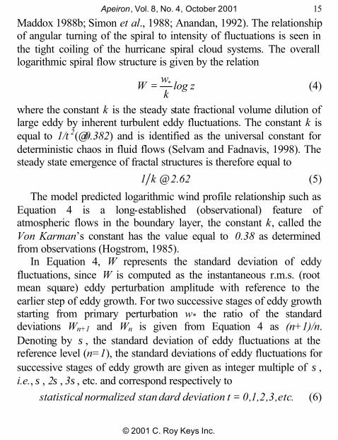
Maddox 1988b; Simon et al., 1988; Anandan, 1992). The relationship of angular turning of the spiral to intensity of fluctuations is seen in the tight coiling of the hurricane spiral cloud systems. The overall logarithmic spiral flow structure is given by the relation

zlogkw

W ∗= (4)

where the constant k is the steady state fractional volume dilution of large eddy by inherent turbulent eddy fluctuations. The constant k is equal to 1/τ2(≅0.382) and is identified as the universal constant for deterministic chaos in fluid flows (Selvam and Fadnavis, 1998). The steady state emergence of fractal structures is therefore equal to

62.2k1 ≅ (5)

The model predicted logarithmic wind profile relationship such as Equation 4 is a long-established (observational) feature of atmospheric flows in the boundary layer, the constant k, called the Von Karman’s constant has the value equal to 0.38 as determined from observations (Hogstrom, 1985).

In Equation 4, W represents the standard deviation of eddy fluctuations, since W is computed as the instantaneous r.m.s. (root mean square) eddy perturbation amplitude with reference to the earlier step of eddy growth. For two successive stages of eddy growth starting from primary perturbation w* the ratio of the standard deviations Wn+1 and Wn is given from Equation 4 as (n+1)/n. Denoting by σ, the standard deviation of eddy fluctuations at the reference level (n=1), the standard deviations of eddy fluctuations for successive stages of eddy growth are given as integer multiple of σ, i.e., σ, 2σ, 3σ, etc. and correspond respectively to .etc,3,2,1,0tdeviationdardtansnormalizedlstatistica = (6)



The conventional power spectrum plotted as the variance versus the frequency in log-log scale will now represent the eddy probability density on logarithmic scale versus the standard deviation of the eddy fluctuations on linear scale since the logarithm of the eddy wavelength represents the standard deviation, i.e., the r.m.s. value of eddy fluctuations (Equation 4). The r.m.s. value of eddy fluctuations can be represented in terms of statistical normal distribution as follows. A normalized standard deviation t=0 corresponds to cumulative percentage probability density equal to 50 for the mean value of the distribution. Since the logarithm of the wavelength represents the r.m.s. value of eddy fluctuations the normalized standard deviation t is defined for the eddy energy as

1)TlogLlog(t 50 −= (7)

where L is the period in years and T50 is the period up to which the cumulative percentage contribution to total variance is equal to 50 and t = 0. The variable LogT50 also represents the mean value for the r.m.s. eddy fluctuations and is consistent with the concept of the mean level represented by r.m.s. eddy fluctuations. Spectra of time series of fluctuations of dynamical systems, for example, meteorological parameters, when plotted as cumulative percentage contribution to total variance versus t follow the model predicted universal spectrum (Selvam and Fadnavis, 1998, and all references therein). The literature shows many examples of pressure, wind and temperature whose shapes display a remarkable degree of universality (Canavero and Einaudi, 1987).

The periodicities (or length scales) T50 and T95 up to which the cumulative percentage contribution to total variances are respectively equal to 50 and 95 are computed from model concepts as follows.

The power spectrum, when plotted as normalised standard deviation t versus cumulative percentage contribution to total variance



represents the statistical normal distribution (Equation 7), i.e., the variance represents the probability density. The normalised standard deviation values t corresponding to cumulative percentage probability densities P equal to 50 and 95 respectively are equal to 0 and 2 from statistical normal distribution characteristics. Since t represents the eddy growth step n (Equation 6) the dominant periodicities (or length scales) T50 and T95 up to which the cumulative percentage contribution to total variance are respectively equal to 50 and 95 are obtained from Equation 3 for corresponding values of n equal to 0 and 2. In the present study of fractal fluctuations of spacing intervals of adjacent Riemann zeta zeros, the primary perturbation length scale Ts is equal to unit spacing interval and T50 and T95 are obtained as

intervals spacing6unit3(2T 050 .≅ττ)+= (8)

intervals spacingunit592(T 295 .≅ττ)+= (9)

3. Data and Analysis Details of the Riemann zeta zeros (non-trivial) used in the present study are given in the following: (a) The first 100000 zeros were obtained from: http://www.research.att.com/~amo/zeta_tables/zeros1 (b) Riemann zeta zeros numbered 1012 + 1 through 1012 + 104 were obtained from: http://www.research.att.com/~amo/zeta_tables/zeros3 [Values of gamma - 267653395647, where gamma runs over the heights of the zeros of the Riemann zeta numbered 1012 + 1 through 1012 + 104. Thus zero # 1012 + 1 is actually 1/2 + i * 267,653,395,648.8475231278... Values are guaranteed to be accurate only to within 10 -8].



(c) Riemann zeta zeros numbered 1021 + 1 through 1021 + 104 were obtained from: http://www.research.att.com/~amo/zeta_tables/zeros4 [Values of gamma - 144176897509546973000, where gamma runs over the heights of the zeros of the Riemann zeta numbered 1021 + 1 through 1021 + 104. Thus zero # 1021 + 1 is actually 1/2 + i * 144,176,897,509,546,973,538.49806962... Values are not guaranteed, and are probably accurate to within 10 -6]. (d) Riemann zeta zeros numbered 1022 + 1 through 1022 + 104 were obtained from: http://www.research.att.com/~amo/zeta_tables/zeros5 [Values of gamma - 1370919909931995300000, where gamma runs over the heights of the zeros of the Riemann zeta numbered 1022 + 1 through 1022 + 104. Thus zero # 1022 + 1 is actually 1/2 + i * 1,370,919,909,931,995,308,226.68016095... Values are not guaranteed, and are probably accurate to within 10 -6].

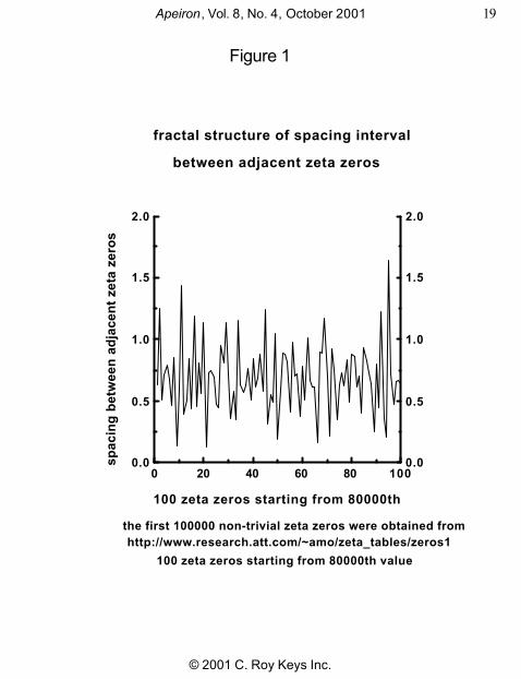
3.1 Fractal structure of spacing intervals of adjacent Riemann zeta zeros

The spacing interval between adjacent zeta zeros for a representative sample of 100 successive zeta zeros starting from the 80,000th value are plotted in Figure 1. The irregular zig-zag pattern of fluctuations of adjacent spacing intervals is identified as characteristic of fractal fluctuations exhibited by dynamical systems, such as, rainfall, river flows, stock market price index, etc. (Selvam and Fadnavis, 1998).



Figure 1

0 20 40 60 80 1000.0

0.5

1.0

1.5

2.0

0.0

0.5

1.0

1.5

2.0

100 zeta zeros starting from 80000th value

http://www.research.att.com/~amo/zeta_tables/zeros1the first 100000 non-trivial zeta zeros were obtained from

between adjacent zeta zeros

fractal structure of spacing interval

spac

ing

bet

wee

n a

dja

cen

t ze

ta z

ero

s

100 zeta zeros starting from 80000th



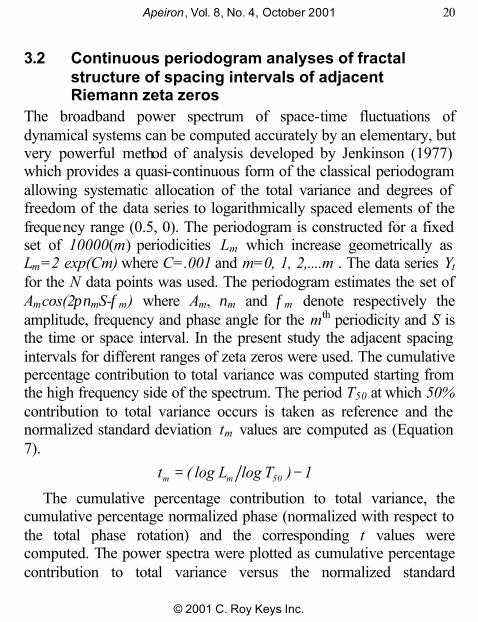
3.2 Continuous periodogram analyses of fractal structure of spacing intervals of adjacent Riemann zeta zeros

The broadband power spectrum of space-time fluctuations of dynamical systems can be computed accurately by an elementary, but very powerful method of analysis developed by Jenkinson (1977) which provides a quasi-continuous form of the classical periodogram allowing systematic allocation of the total variance and degrees of freedom of the data series to logarithmically spaced elements of the frequency range (0.5, 0). The periodogram is constructed for a fixed set of 10000(m) periodicities Lm which increase geometrically as Lm=2 exp(Cm) where C=.001 and m=0, 1, 2,....m . The data series Yt for the N data points was used. The periodogram estimates the set of Amcos(2πνmS-φm) where Am, νm and φm denote respectively the amplitude, frequency and phase angle for the mth periodicity and S is the time or space interval. In the present study the adjacent spacing intervals for different ranges of zeta zeros were used. The cumulative percentage contribution to total variance was computed starting from the high frequency side of the spectrum. The period T50 at which 50% contribution to total variance occurs is taken as reference and the normalized standard deviation tm values are computed as (Equation 7).

1)TlogLlog(t 50mm −=

The cumulative percentage contribution to total variance, the cumulative percentage normalized phase (normalized with respect to the total phase rotation) and the corresponding t values were computed. The power spectra were plotted as cumulative percentage contribution to total variance versus the normalized standard



deviation t as given above. The period L is in units of number of class intervals, unit class interval being equal to adjacent spacing interval of zeta zeros in the present study. Periodicities up to T50 contribute up to 50% of total variance. The phase spectra were plotted as cumulative percentage normalized (normalized to total rotation) phase .

Five groups of data sets (zeros5, zeros4, zeros3, zeros1a and zeros1b) were used. Details of these five data sets are: (i) The first three data groups, namely, zeros5, zeros4, zeros3 consist of the following thirteen data sets of the same length located at same locations in the three data files zeros5, zeros4, and zeros3 respectively (1) 1 to100 (2) 1 to 500 (3) 1 to 1000 (4) 1 to 1500 (5) 1 to 2000 (6) 1 to 3000 (7) 1 to 4000 (8) 1 to 5000 (9) 5000 to 5099 (10) 5000 to 5499 (11) 5000 to 5999 (12) 5000 to 6499 (13) 1 to 9999. (ii) The data group zeros1a consists of the first twelve data sets shown above for the first three data groups at corresponding locations in data file zeros1. (iii) The data group zeros1b consists of the following eight data sets located in data file zeros1 (1) 5000 to 14999 (2) 5000 to 9999 (3) 10000 to 19999 (4) 80000 to 89999 (5) 80000 to 80099 (6) 98000 to 98049 (7) 98009 to 98049 (8) file zeros3, 5000 to 5049.

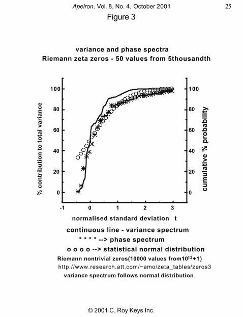
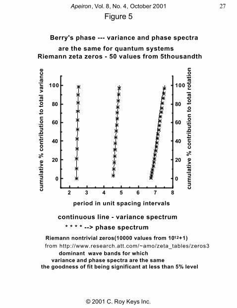
The results of power spectral analyses for all the data sets are shown in Figures 2 to 9. The variance and phase spectra along with statistical normal distributions are shown in Figures 2 and 3 for two representative data sets of Riemann zeta zero spacing intervals. Also, for these two representative data sets, the cumulative percentage contribution to total variance and the cumulative (%) normalized phase (normalized with respect to. the total rotation) for each dominant waveband is computed for significant wavebands and shown in Figures 4 and 5 to illustrate Berry’s phase, namely the progressive increase in phase with increase in period and also the close association between phase and variance (see Section 2)



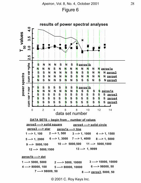
Figure 6 shows the following: (a) details of data files (b) data series location in the data file (c) number of data values in each series (d) the value of T50 which is the length scale up to which the cumulative percentage contribution to total variance is equal to 50 (in unit spacing intervals of Riemann zeta zeros). (e) whether the variance and phase spectra follow statistical normal distribution characteristics. The length of the data sets ranged from 50 to 10,000 values.

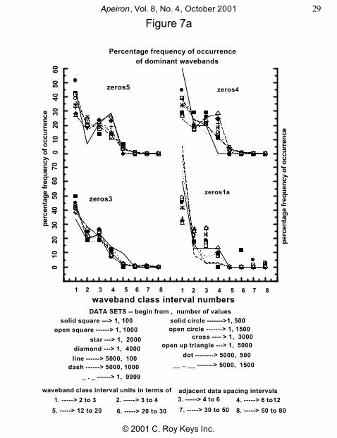
Figures 7 to 9 give the following additional results for the same data sets grouped according to frequency of occurrence of dominant wavebands with peak periodicities in class intervals 2 - 3, 3 - 4, 4 - 6, 6 - 12, 12 - 20, 20 - 30, 30 - 50, 50 – 80. These wavebands include the model predicted (Equation 3) dominant peak periodicities (or length scales) 2.2, 3.6, 5.8, 9.5, 15.3, 24.8, 40.1, and 64.9 (in unit spacing intervals of Riemann zeta zeros) for values of n ranging from -1 to 6. Figures 7a and 7b show the percentage number of dominant wavebands. Figures 8a and 8b show the percentage number of statistically significant (less than or equal to 5% level) dominant wavebands. Figures 9a and 9b show the percentage number of dominant wavebands, which exhibit Berry’s phase, namely, the variance spectrum follows closely the phase spectrum (see Section 2).

3.3 Results of power spectral analyses Results of power spectral analyses of Riemann zeta zero spacing

intervals agree with the following model predictions: (a) almost all variance spectra follow statistical normal distribution (Figure 6) (b) The magnitude of T50 values (Figure 6) are very close to model predicted value of 3.6 unit spacing intervals (see equation 8).

The ‘goodness of fit’ (statistical chi-square test) between the variance spectrum and statistical normal distribution is significant at less than or equal to 5% level for the two representative spectra



shown in Figures 2 and 3 and also for almost all the data sets shown by the symbol S in Figure 6. The phase spectrum is close to the statistical normal distribution, but the ‘goodness of fit ’ is not statistically significant in a majority of cases as shown by the symbol N in Figure 6. However, the ‘goodness of fit ‘ between variance and phase spectra illustrating Berry’s phase is statistically significant (chi-square test) for individual dominant wavebands, particularly for longer periodicities (Figures 4 and 5 and Figures 9a and 9b). The frequency of occurrence of shorter dominant periodicities up to 5 spacing interval units is a maximum as compared to longer periodicities (Figures 7a and 7b). Also a majority of shorter dominant periodicities up to 5 spacing interval units are found to be statistically significant (Figures 8a and 8b). The predominance of shorter dominant periodicities is consistent with model predicted and observed (Figure 6) value of about 3.6 for the value of T50 which is the period up to which the cumulative percentage contribution to total variance is equal to 50.



Figure 2

-1 0 1 2 3

0

20

40

60

80

100

0

20

40

60

80

100

variance spectrum follows normal distribution

o o o o --> statistical normal distribution

* * * * --> phase spectrum

continuous line - variance spectrum

http://www.research.att.com/~amo/zeta_tables/zeros1Riemann nontrivial zeros(first 100000) obtained from

variance and phase spectra

cum

ula

tive

% p

rob

abili

ty

Riemann zeta zeros - 50 values from 98thousandth

% c

on

trib

uti

on

to

to

tal v

aria

nce

normalised standard deviation t



Figure 3

-1 0 1 2 3

0

20

40

60

80

100

0

20

40

60

80

100

Riemann nontrivial zeros(10000 values from1012+1)

variance spectrum follows normal distribution

http://www.research.att.com/~amo/zeta_tables/zeros3

o o o o --> statistical normal distribution* * * * --> phase spectrum


Riemann zeta zeros - 50 values from 5thousandthvariance and phase spectra

cum

ula

tive

% p

rob

abili

ty

normalised standard deviation t

% c

on

trib

uti

on

to

to

tal v

aria

nce



Figure 4

2 3 4 5 6 7 8 9

0

20

40

60

80

100

0

20

40

60

80

100

Riemann zeta zeros - 50 values from 98thousandth

the goodness of fit being significant at less than 5% level

are the same for quantum systems

dominant wave wave bands for whichvariance and phase spectra are the same

http://www.research.att.com/~amo/zeta_tables/zeros1

Riemann nontrivial zeros(first 100000) obtained from



Berry's phase --- variance and phase spectra

cum

ula

tive

% c

on

trib

utio

n to

tota

l ro

tatio

n

cum

ulat

ive

% c

ontr

ibut

ion

to to

tal v

aria

nce

period in unit spacing intervals



Figure 5

2 3 4 5 6 7 8

0

20

40

60

80

100

0

20

40

60

80

100

from http://www.research.att.com/~amo/zeta_tables/zeros3

the goodness of fit being significant at less than 5% levelvariance and phase spectra are the same

dominant wave bands for which

Riemann nontrivial zeros(10000 values from 1012+1)



period in unit spacing intervals

cum

ula

tive

% c

on

trib

uti

on

to

to

tal v

aria

nce

cum

ula

tive

% c

on

trib

uti

on

to

to

tal r

ota

tio

n

Riemann zeta zeros - 50 values from 5thousandthare the same for quantum systems

Berry's phase --- variance and phase spectra



Figure 6

0 2 4 6 8 10 12 14

results of power spectral analyses

S N N N S N S S zeros1bN N N S N N N N N N N N zeros1aS S N N N N S N S S N N N zeros3S S N N N N S S N N N N N zeros4N S N N S N N S S S N S N zeros5

S S S S S S S S zeros1bN N N N N N N S S S S S zeros1aS S S S S S S S S S S S S zeros3S S S S S S S S S S S S S zeros4

cum

var

=ph

scu

m v

ar =

nor

pow

er s

pect

ra

2.5

3

.0

3.5

4

.0

S S S S S S S S S S S S S zeros5

13 ---> 1, 999912 ---> 5000,1500

11 ---> 5000,100010 ---> 5000,5009 ---> 5000,100

8 ---> 1, 50006 ---> 1, 3000 7 ---> 1, 40005 ---> 1, 2000

4 ---> 1, 15003 ---> 1, 10002 ---> 1, 5001 ---> 1, 100

8 ----> zeros3, 5000, 507 ----> 98009, 50

6 ----> 98000, 505 ----> 80000, 100004 ----> 80000, 100

3 ----> 10000, 100002 -----> 5000, 100001 ----> 5000, 5000

DATA SETS -- begin from , number of values

zeros1b ----> dot

zeros1a ----> linezeros3 ----> starzeros4 ----> solid circlezeros5 ----> solid square

T 50 v

alue

s

data set number



Figure 7a

0

10

20

30

40

50

6

0

1 2 3 4 5 6 7 8

of dominant wavebandsPercentage frequency of occurrence

perc

enta

ge fr

eque

ncy

of o

ccur

renc

e

perc

enta

ge fr

eque

ncy

of o

ccur

renc

e0

10

2

0

30

40

50

6

0

70

1 2 3 4 5 6 7 8

adjacent data spacing intervalswaveband class interval units in terms of

8. -----> 50 to 807. -----> 30 to 506. -----> 20 to 305. -----> 12 to 20

4. -----> 6 to123. -----> 4 to 62. -----> 3 to 41. -----> 2 to 3

_ . _ ------> 1, 9999


__ .. __ -------> 5000, 1500dash ------> 5000, 1000

dot --------> 5000, 500line ------> 5000, 100

open square ------> 1, 1000solid square ---> 1, 100

zeros1azeros3

zeros4zeros5

open up triangle ---> 1, 5000diamond ---> 1, 4000

cross ---- > 1, 3000star ---> 1, 2000

open circle -------> 1, 1500solid circle ------->1, 500

waveband class interval numbers



Figure 7b

0 2 4 6 8-10

0

10

20

30

40

50

60

70

80

90

-10

0

10

20

30

40

50

60

70

80

90

perc

enta

ge fr

eque

ncy

of o

ccur

renc

e

of dominant wavebandsPercentage frequency of occurrence

1. -----> 2 to 3

8. -----> 50 to 807. -----> 30 to 50

6. -----> 20 to 305. -----> 12 to 204. -----> 6 to12

3. -----> 4 to 62. -----> 3 to 4adjacent data spacing intervals

waveband class interval units in terms of

DATA SETS -- begin from , number of valueswaveband class interval numbers

line ----> zeros3, 5000, 50

up triangle open ----> 98009, 50

cross ----> 98000, 50

open circle ----> 80000, 100

open square ----> 80000, 10000

star ----> 10000, 10000

solid circle ----> 5000, 5000

zeros1b

solid square -----> 5000, 10000



Figure 8a

0

20

4

0

60

8

0

100

0

20

4

0

60

8

0

100

0

20

4

0

60

8

0

100

significant dominant wavebands

percentage frequency of statistically

zeros1azeros3

zeros4zeros5

0

20

4

0

60

8

0

100

1 2 3 4 5 6 7 81 2 3 4 5 6 7 8

perc

enta

ge fr

eque

ncy

of o

ccur

renc

e


8. -----> 50 to 807. -----> 30 to 506. -----> 20 to 305. -----> 12 to 204. -----> 6 to 123. -----> 4 to 62. -----> 3 to 41. -----> 2 to 3


short _._ ----> 1, 9999__..__ -----> 5000, 1500

dash ----> 5000, 1000dot ----> 5000, 500

line ----> 5000, 100open up triangle ----> 1, 5000

diamond ----> 1, 4000cross ----> 1, 3000star ----> 1, 2000

open circle ----> 1, 1500open square ----> 1, 1000solid circle ----> 1, 500solid square ---> 1, 100




Figure 8b

0 2 4 6 8

0

20

40

60

80

100

0

20

40

60

80

100

zeros1b

significant dominant wavebandspercentage frequency of statistically

perc

enta

ge fr

eque

ncy

of o

ccur

renc

e

8. -----> 50 to 807. -----> 30 to 50

6. -----> 20 to 305. -----> 12 to 204. -----> 6 to 12

3. -----> 4 to 62. -----> 3 to 41. -----> 2 to 3


line ----> zeros3, 5000, 50

up triangle open ----> 98009, 50

cross ----> 98000, 50

open square ----> 80000, 10000

open circle ----> 80000, 100

star ----> 10000, 10000

solid square -----> 5000, 10000

solid circle ----> 5000, 5000





Figure 9a

0

20

4

0

60

8

0

100

1 2 3 4 5 6 7 8

which exhibit Berry's phasepercentage of dominant wavebands

zeros3

zeros1a

8. -----> 50 to 807. -----> 30 to 506. -----> 20 to 305. -----> 12 to 20

4. -----> 6 to 123. -----> 4 to 62. -----> 3 to 41. -----> 2 to 3adjacent data spacing intervalswaveband class interval units in terms of


0

20

4

0

60

8

0

100

0

20

4

0

60

8

0

100

0

20

4

0

60

8

0

100

1 2 3 4 5 6 7 8waveband class interval numbers

perc

enta

ge fr

eque

ncy

of o

ccur

renc

e

zeros4

short _._ ----> 1, 9999

__..__ -----> 5000, 1500dash ----> 5000, 1000

dot ----> 5000, 500line ----> 5000, 100

open up triangle ----> 1, 5000

diamond ----> 1, 4000cross ----> 1, 3000star ----> 1, 2000open circle ----> 1, 1500open square ----> 1, 1000solid circle ----> 1, 500solid square ---> 1, 100

zeros5



Figure 9b

0 2 4 6 8

0

20

40

60

80

100

0

20

40

60

80

100

zeros1b


perc

enta

ge fr

eque

ncy

of o

ccur

renc

ewhich exhibit Berry's phase

percentage of dominant wavebands

8. -----> 50 to 807. -----> 30 to 50

6. -----> 20 to 305. -----> 12 to 204. -----> 6 to 12

3. -----> 4 to 62. -----> 3 to 41. -----> 2 to 3


line ----> zeros3, 5000, 50up triangle open ----> 98009, 50

cross ----> 98000, 50open square ----> 80000, 10000

open circle ----> 80000, 100star ----> 10000, 10000

solid square -----> 5000, 10000solid circle ----> 5000, 5000




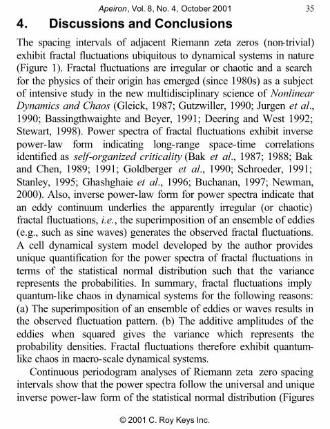
4. Discussions and Conclusions The spacing intervals of adjacent Riemann zeta zeros (non-trivial) exhibit fractal fluctuations ubiquitous to dynamical systems in nature (Figure 1). Fractal fluctuations are irregular or chaotic and a search for the physics of their origin has emerged (since 1980s) as a subject of intensive study in the new multidisciplinary science of Nonlinear Dynamics and Chaos (Gleick, 1987; Gutzwiller, 1990; Jurgen et al., 1990; Bassingthwaighte and Beyer, 1991; Deering and West 1992; Stewart, 1998). Power spectra of fractal fluctuations exhibit inverse power-law form indicating long-range space-time correlations identified as self-organized criticality (Bak et al., 1987; 1988; Bak and Chen, 1989; 1991; Goldberger et al., 1990; Schroeder, 1991; Stanley, 1995; Ghashghaie et al., 1996; Buchanan, 1997; Newman, 2000). Also, inverse power-law form for power spectra indicate that an eddy continuum underlies the apparently irregular (or chaotic) fractal fluctuations, i.e., the superimposition of an ensemble of eddies (e.g., such as sine waves) generates the observed fractal fluctuations. A cell dynamical system model developed by the author provides unique quantification for the power spectra of fractal fluctuations in terms of the statistical normal distribution such that the variance represents the probabilities. In summary, fractal fluctuations imply quantum-like chaos in dynamical systems for the following reasons: (a) The superimposition of an ensemble of eddies or waves results in the observed fluctuation pattern. (b) The additive amplitudes of the eddies when squared gives the variance which represents the probability densities. Fractal fluctuations therefore exhibit quantum-like chaos in macro-scale dynamical systems.

Continuous periodogram analyses of Riemann zeta zero spacing intervals show that the power spectra follow the universal and unique inverse power-law form of the statistical normal distribution (Figures



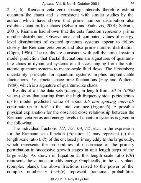
2, 3, 6). Riemann zeta zero spacing intervals therefore exhibit quantum-like chaos and is consistent with similar studies by the author, which have shown that prime number distribution also exhibits quantum-like chaos (Selvam and Fadnavis, 2001; Selvam, 2001). Riemann had shown that the zeta function represents prime number distribution. Observational and computed values of energy level distributions of excited quantum systems appear to follow closely the Riemann zeta zeros and also prime number distribution (Cipra, 1996). The results are consistent with cell dynamical system model prediction that fractal fluctuations are signatures of quantum-like chaos in dynamical systems of all sizes ranging from the sub-atomic quantum systems to macro-scale fluid flows. The Heisenberg uncertainty principle for quantum systems implies unpredictable fluctuations, i.e., fractal space-time fluctuations (Hey and Walters, 1989), which is a signature of quantum-like chaos.

Results of all the data sets (ranging in length from 50 to 10000 values) show that starting from the high frequency side, periodicities up to model predicted value of about 3.6 unit spacing intervals contribute up to 50% to the total variance (Figure 6). A possible physical explanation for the observed close relationship between the Riemann zeta zeros and energy levels of quantum systems is given in the following:

The individual fractions 1/2, 1/3, 1/4, 1/5, etc., in the expression for the Riemann zeta function (Equation 1) may represent (a) the length scale ratio (r/R) of the enclosed primary eddy to the large eddy, which represents the probabilities of occurrence of the primary perturbation in successive growth stages in unit length steps of the large eddy. As shown in Equation 2, this length scale ratio (r/R) represents the variance or eddy energy. Graphically, in the x - y plane (complex plane), the above fractions raised to the power of the complex number s (=x+iy) represent fractional probabilities



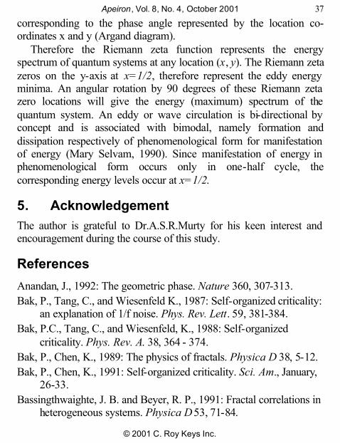
corresponding to the phase angle represented by the location co-ordinates x and y (Argand diagram).

Therefore the Riemann zeta function represents the energy spectrum of quantum systems at any location (x, y). The Riemann zeta zeros on the y-axis at x=1/2, therefore represent the eddy energy minima. An angular rotation by 90 degrees of these Riemann zeta zero locations will give the energy (maximum) spectrum of the quantum system. An eddy or wave circulation is bi-directional by concept and is associated with bimodal, namely formation and dissipation respectively of phenomenological form for manifestation of energy (Mary Selvam, 1990). Since manifestation of energy in phenomenological form occurs only in one-half cycle, the corresponding energy levels occur at x=1/2.

5. Acknowledgement The author is grateful to Dr.A.S.R.Murty for his keen interest and encouragement during the course of this study.

References

Anandan, J., 1992: The geometric phase. Nature 360, 307-313. Bak, P., Tang, C., and Wiesenfeld K., 1987: Self-organized criticality:

an explanation of 1/f noise. Phys. Rev. Lett. 59, 381-384. Bak, P.C., Tang, C., and Wiesenfeld, K., 1988: Self-organized

criticality. Phys. Rev. A. 38, 364 - 374. Bak, P., Chen, K., 1989: The physics of fractals. Physica D 38, 5-12. Bak, P., Chen, K., 1991: Self-organized criticality. Sci. Am., January,

26-33. Bassingthwaighte, J. B. and Beyer, R. P., 1991: Fractal correlations in

heterogeneous systems. Physica D 53, 71-84.



Berry, M. V., 1988: The geometric phase. Sci. Amer. Dec., 26-32. Berry, M., 1992: Quantum physics on the edge of chaos. In The New

Scientist ’s Guide to Chaos, (Ed) Nina Hall, Penguin Books, pp.184 - 195.

Buchanan, M., 1997: One law to rule them all. New Scientist 8 Nov., 30-35.

Burroughs, W. J., 1992: Weather Cycles: Real or Imaginary? Cambridge University Press, Cambridge.

Canavero, F. G., Einaudi, F.,1987: Time and space variability of atmospheric processes. J. Atmos. Sci. 44(12), 1589-1604.

Capra, F., 1996: The web of life, HarperCollins Publishers, London, pp.311.

Cipra, B., 1996: Prime formula weds number theory and quantum physics. Science 274, 2014-2015.

Deering, W., and West, B. J., 1992: Fractal physiology. IEEE Engineering in Medicine and Biology, June, 40-46.

Devlin, K., 1997: Mathematics: The Science of Patterns. Scientific American Library, New York, pp.215.

Ghashghaie, S., Breymann, Peinke, J., Talkner, P., Dodge, Y., 1996: Turbulent cascades in foreign exchange markets. Nature 381, 767-770.

Ghil, M., 1994: Cryothermodynamics: the chaotic dynamics of paleoclimate. Physica D 77,130-159.

Gleick, J., 1987: Chaos: Making a New Science. Viking, New York. Goldberger, A. L., Rigney, D. R., West, B. J., 1990: Chaos and

fractals in human physiology. Sci. Am. 262(2), 42-49. Gutzwiller, M. C., 1990: Chaos in classical and quantum systems.

Interdisciplinary Applied Mathematics, Volume 1, Springer-Verlag, New York, pp.427.



Hey, T. and Walters, P., 1989: The quantum universe. Cambridge University Press, pp.180.

Hogstrom, U., 1985: Von Karman’s constant in atmospheric boundary layer now re-evaluated. J. Atmos. Sci. 42, 263-270.

Jenkinson, A. F., 1977: A Powerful Elementary Method of Spectral Analysis for use with Monthly, Seasonal or Annual Meteorological Time Series. Meteorological Office, London, Branch Memorandum No. 57, pp. 1-23.

Jurgen, H., Peitgen, H-O, Saupe, D., 1990: The language of fractals. Sci. Amer. 263, 40-49.

Keating, J., 1990: Physics and the queen of mathematics. Physics World April, 46-50.

Klarreich, E., 2000: Prime time. New Scientist 11 November, 32- 36. Maddox, J., 1988a: Licence to slang Copenhagen? Nature 332, 581. Maddox, J., 1988b: Turning phases into frequencies. Nature 334, 99. Maddox, J., 1993: Can quantum theory be understood? Nature 361,

493. Mary Selvam, A., 1990: Deterministic chaos, fractals and

quantumlike mechanics in atmospheric flows. Can. J. Phys. 68, 831-841. http://xxx.lanl.gov/html/physics/0010046

Newman, M., 2000: The power of design. Nature 405, 412-413. Rae, A., 1988: Quantum-physics: illusion or reality? Cambridge

University Press, New York, p.129. Richards, D., 1988: Order and chaos in strong fields. Nature 336,

518-519. Ruhla, C., 1992: The physics of chance. Oxford University Press,

Oxford, U. K., pp.217. Schroeder, M., 1991: Fractals, Chaos and Powerlaws. W. H.

Freeman and Co., N.Y.



Selvam, A. M., and Fadnavis, S., 1998: Signatures of a universal spectrum for atmospheric interannual variability in some disparate climatic regimes. Meteorology and Atmospheric Physics 66, 87-112. http://xxx.lanl.gov/abs/chao-dyn/9805028

Selvam, A. M., and Fadnavis, S., 2001: Cantorian fractal patterns, quantum-like chaos and prime numbers in atmospheric flows.(to be submitted for Journal publication). http://xxx.lanl.gov/abs/chao-dyn/9810011

Selvam, A. M., 2001: Quantum-like chaos in prime number distribution and in turbulent fluid flows. Apeiron 8(3), 29-64, (2001). http://redshift.vif.com/ http://xxx.lanl.gov/html/physics/0005067

Simon, R., Kimble, H. J., Sudarshan, E. C. G., 1988: Evolving geometric phase and its dynamical interpretation as a frequency shift: an optical experiment. Phys. Rev. Letts. 61(1), 19-22.

Stanley, H. E., 1995: Powerlaws and universality. Nature 378, 554. Stewart, I., 1998: Life’s other secret . Allen Lane, The penguin press,

pp.273.

signatures of quantum-like chaos in spacing intervals of non

Documents