silt fences: an economical technique for measuring ... fences: an economical technique for measuring...
TRANSCRIPT

Silt Fences: An Economical Technique
for Measuring Hillslope Soil Erosion
Peter R. Robichaud
Robert E. Brown
United StatesDepartmentof Agriculture
Forest Service
Rocky MountainResearch Station
General TechnicalReport RMRS-GTR-94
August 2002

Robichaud, Peter R.; Brown, Robert E. 2002. Silt fences: an economical technique for measuringhillslope soil erosion. Gen. Tech. Rep. RMRS-GTR-94. Fort Collins, CO: U.S. Department of Agriculture,Forest Service, Rocky Mountain Research Station. 24 p.
Abstract—Measuring hillslope erosion has historically been a costly, time-consuming practice. An easy toinstall low-cost technique using silt fences (geotextile fabric) and tipping bucket rain gauges to measureonsite hillslope erosion was developed and tested. Equipment requirements, installation procedures, statis-tical design, and analysis methods for measuring hillslope erosion are discussed. The use of silt fences isversatile; various plot sizes can be used to measure hillslope erosion in different settings and to determineeffectiveness of various treatments or practices. Silt fences are installed by making a sediment trap facingupslope such that runoff cannot go around the ends of the silt fence. The silt fence is folded to form a pocketfor the sediment to settle on and reduce the possibility of sediment undermining the silt fence. Cleaning outand weighing the accumulated sediment in the field can be accomplished with a portable hanging or plat-form scale at various time intervals depending on the necessary degree of detail in the measurement oferosion (that is, after every storm, quarterly, or seasonally). Silt fences combined with a tipping bucket raingauge provide an easy, low-cost method to quantify precipitation/hillslope erosion relationships. Trap effi-ciency of the silt fences are greater that 90 percent efficient, thus making them suitable to estimate hillslopeerosion.
Keywords—silt fence, erosion, erosion rate, sediment, measurement techniques, monitoring
The Authors
Peter R. Robichaud is a Research Engineer and Robert E. Brown is a Hydrologist with the Soil and WaterEngineering Research Work Unit, Rocky Mountain Research Station, Forestry Sciences Laboratory, 1221South Main St., Moscow, ID 83843.
Acknowledgments
Many individuals assisted in installation of silt fences over the years. This includes personnel from theSoil and Water Engineering Project as well as various National Forest personnel. David Turner, Statisticianwith the Rocky Mountain Research Station, provided statistical assistance.
Contents
Introduction ............................................................................................................................ 1
Site Selection .......................................................................................................................... 2
Defining Contributing Areas to Silt Fence....................................................................... 2
Silt Fence Plot Installation .................................................................................................... 4
Cleanout, Maintenance, and Schedule .................................................................................. 5
Additional Data Collection ..................................................................................................... 5
Precipitation Measurements ............................................................................................. 5
Ground Cover Measurements ........................................................................................... 7
Data Analysis and Interpretation: Statistical Design .......................................................... 7
Summary ................................................................................................................................. 8
References ............................................................................................................................... 8
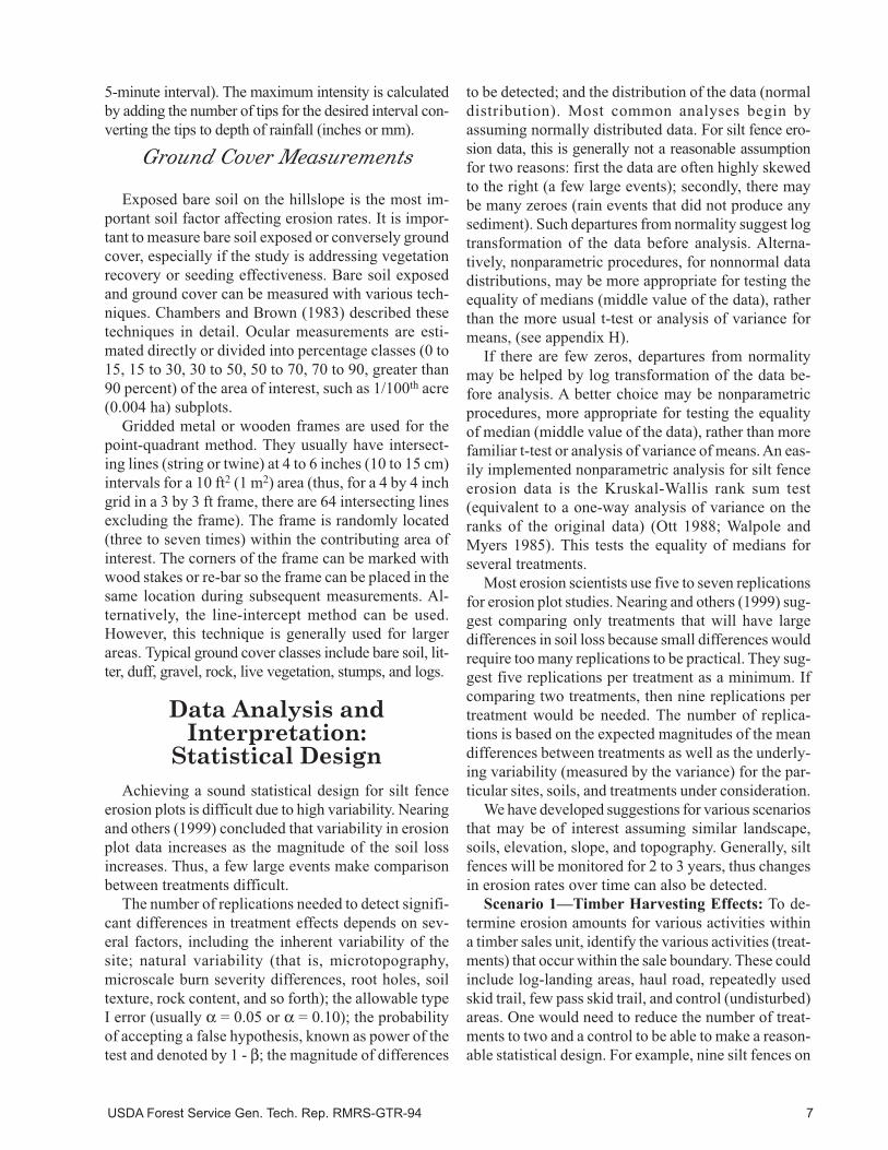
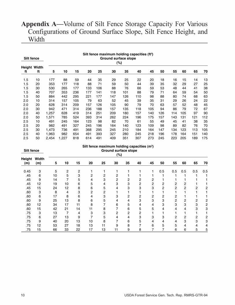
Appendix A—Volume of Silt Fence Storage Capacity For Various Configurations of
Ground Surface Slope, Silt Fence Height, and Width ................................................... 10
Appendix B—Common Silt Fence Specifications ................................................................ 11
Appendix C—List of Suppliers for Silt Fences and Rain Gauges ...................................... 13
Appendix D—Equipment List .............................................................................................. 16
Appendix E—Example of Field Data Sheet ........................................................................ 17
Appendix F—Example of Field and Laboratory Spreadsheet ............................................ 18
Appendix G—Example Data Taken From Onset Rain Gauge Datalogger ....................... 19
Appendix H—Statistical Analysis Procedure ..................................................................... 20

USDA Forest Service Gen. Tech. Rep. RMRS-GTR-94 1
Introduction
Soil erosion is a major land management issue due
to stringent regulations on water quality and efforts to
reduce the impact of various activities on sedimenta-
tion. Surface erosion is the movement of individual
soil particles by a force, either by uniform removal of
material from the soil surface (sheet erosion) or by
concentrated removal of material in the downslope di-
rection (rill erosion) (Foster 1982). Forces required to
initiate and sustain the movement of soil particles can
be from many sources, such as raindrop impact, over-
land flow, gravity, wind, and animal activity. Erosion
is a natural process; however, human or natural distur-
bances on the landscape generally increase surface ero-
sion over natural levels. Erosion is reduced by all ma-
terial on or above the soil surface, such as naturally
occurring vegetation, surface litter, duff, rocks, and
synthetic materials such as erosion mats, mulches, and
other barriers that reduce the impact of the applied
forces (McNabb and Swanson 1990; Megahan and
others 1986).
Erosion modeling techniques have been developed
to predict erosion following common disturbances.
Some of these models are not receiving widespread
use probably because they were not developed or vali-
dated for a particular condition or treatment of inter-
est. Therefore, many government agencies, farmers,
industries, and consultants need an easy method to
measure hillslope erosion to validate model results as
well as need local information from their particular
conditions.
Soil erosion measuring techniques can be costly and
time consuming. Various techniques have been used
including rainfall simulation, erosion bridges, Gerlach
troughs, and small watershed measurement techniques.
Dissmeyer (1982) developed a protocol to measure
hillslope erosion with silt fences. His techniques have
been utilized and improved upon in this document. Less
expensive data recording equipment (such as, continu-
ous recording tipping bucket rain gauges) has made it
easier for land managers to obtain their own erosion
rate data as well as information on the type of storms
that caused the erosion. This information can be used for
completing environmental assessment documentation.
Silt fences have been used to control surface ero-
sion in the construction industry for several decades.
Also, silt fences have been used for instream sediment
control (Trow Consulting Engineers Ltd. 1996). A silt
fence is a synthetic geotextile fabric that is woven to
provide structural integrity (tensile strength 80 to 100
lb, 0.3 to 0.4 kN) with small openings (0.01 to 0.03
inch, 0.3 to 0.8 mm) that pass water but not sediment.
Silt fences have low permeability rates, which make
them suitable to form temporary detention storage ar-
eas allowing sediment to settle and water to pass
through slowly.
Hydraulic performance of silt fences has been mea-
sured by several researchers using flume studies
(Britton and others 2000, 2001; Jiang and others 1996).
They concluded that the maximum flow rate through
silt fences is a function of the head and is generally
small (0.01 to 0.46 ft3 sec-1or 0.00028 to 0.013 m3 sec-1).
Flume studies have shown silt fence trap efficiencies
ranging from 68 to 98 percent (Britton and others 2000,
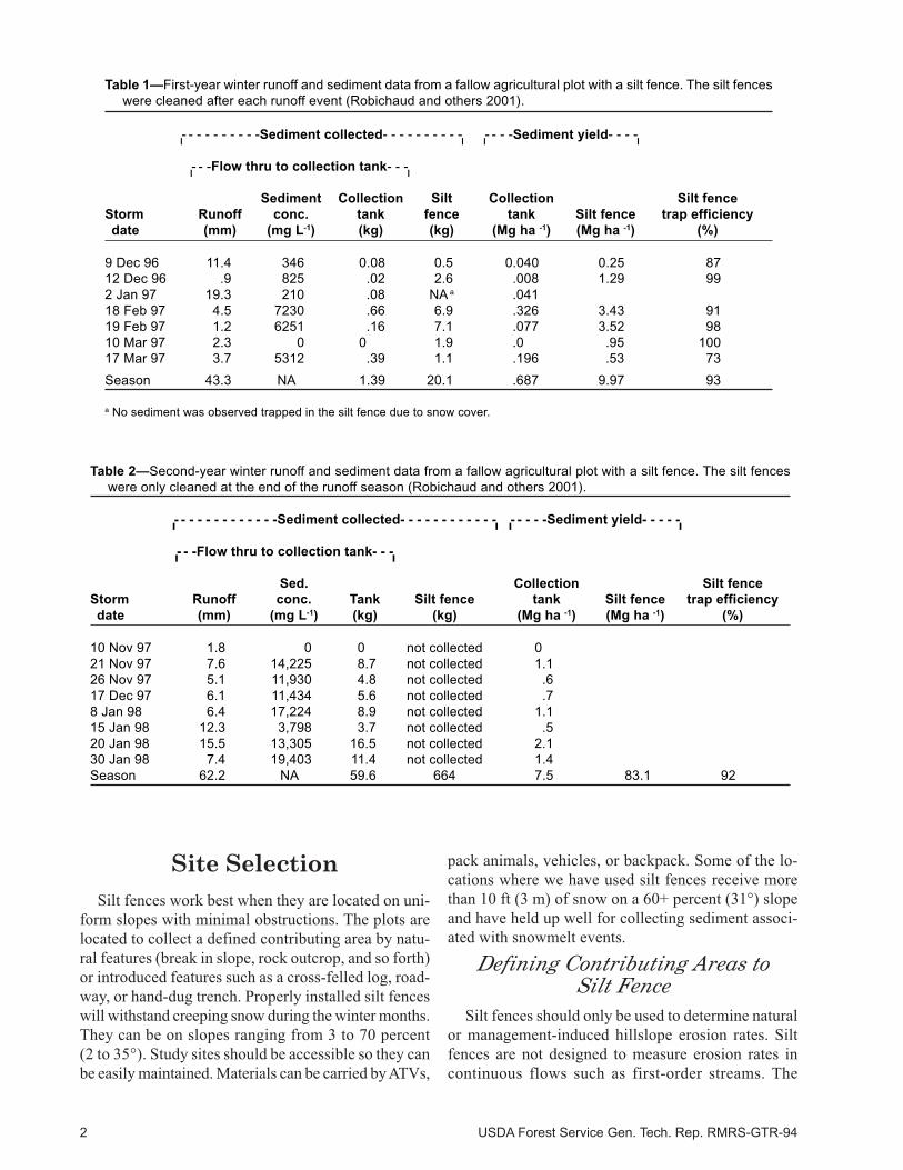
2001; Wishowski and others 1998; Wyant 1980). A field
study of silt fence trap efficiency on an existing long-
term hillslope erosion plot at the Agricultural Re-
search Service Palouse Conservation Field Station
in Washington with a Palouse silt loam soil indicated
trap efficiency was 93 percent the first year when mea-
sured on a storm-by-storm basis and 92 percent effi-
cient the second year when only measured at the end
of the runoff season (Robichaud and others 2001)
(tables 1 and 2).
This paper describes how erosion measurements can
be made with silt fences. Installation procedures, sta-
tistical design, analysis methods, and equipment re-
quirements are discussed. Silt fences can be used to
compare erosion effects of silvicultural treatments,
farming practices, grazing systems, road or skid trail
erosion, vegetative or mechanical rehabilitation treat-
ments, prescribed fires, and wildfires, as well as com-
pare rates of naturally occurring erosion.
Silt Fences: An Economical Technique for
Measuring Hillslope Soil Erosion
Peter R. RobichaudRobert E. Brown
2 USDA Forest Service Gen. Tech. Rep. RMRS-GTR-94
Table 1—First-year winter runoff and sediment data from a fallow agricultural plot with a silt fence. The silt fences
were cleaned after each runoff event (Robichaud and others 2001).
ı- - - - - - - - - -Sediment collected- - - - - - - - - -ı ı- - - -Sediment yield- - - -ı
ı- - -Flow thru to collection tank- - -ı
Sediment Collection Silt Collection Silt fence
Storm Runoff conc. tank fence tank Silt fence trap efficiency
date (mm) (mg L-1) (kg) (kg) (Mg ha -1) (Mg ha -1) (%)
9 Dec 96 11.4 346 0.08 0.5 0.040 0.25 87
12 Dec 96 .9 825 .02 2.6 .008 1.29 99
2 Jan 97 19.3 210 .08 NA a .041
18 Feb 97 4.5 7230 .66 6.9 .326 3.43 91
19 Feb 97 1.2 6251 .16 7.1 .077 3.52 98
10 Mar 97 2.3 0 0 1.9 .0 .95 100
17 Mar 97 3.7 5312 .39 1.1 .196 .53 73
Season 43.3 NA 1.39 20.1 .687 9.97 93
a No sediment was observed trapped in the silt fence due to snow cover.
Table 2—Second-year winter runoff and sediment data from a fallow agricultural plot with a silt fence. The silt fences
were only cleaned at the end of the runoff season (Robichaud and others 2001).
ı- - - - - - - - - - - - -Sediment collected- - - - - - - - - - - -ı ı- - - - -Sediment yield- - - - -ı
ı- - -Flow thru to collection tank- - -ı
Sed. Collection Silt fence
Storm Runoff conc. Tank Silt fence tank Silt fence trap efficiency
date (mm) (mg L-1) (kg) (kg) (Mg ha -1) (Mg ha -1) (%)
10 Nov 97 1.8 0 0 not collected 0
21 Nov 97 7.6 14,225 8.7 not collected 1.1
26 Nov 97 5.1 11,930 4.8 not collected .6
17 Dec 97 6.1 11,434 5.6 not collected .7
8 Jan 98 6.4 17,224 8.9 not collected 1.1
15 Jan 98 12.3 3,798 3.7 not collected .5
20 Jan 98 15.5 13,305 16.5 not collected 2.1
30 Jan 98 7.4 19,403 11.4 not collected 1.4
Season 62.2 NA 59.6 664 7.5 83.1 92
Site Selection
Silt fences work best when they are located on uni-
form slopes with minimal obstructions. The plots are
located to collect a defined contributing area by natu-
ral features (break in slope, rock outcrop, and so forth)
or introduced features such as a cross-felled log, road-
way, or hand-dug trench. Properly installed silt fences
will withstand creeping snow during the winter months.
They can be on slopes ranging from 3 to 70 percent
(2 to 35∞). Study sites should be accessible so they can
be easily maintained. Materials can be carried by ATVs,
pack animals, vehicles, or backpack. Some of the lo-
cations where we have used silt fences receive more
than 10 ft (3 m) of snow on a 60+ percent (31∞) slope
and have held up well for collecting sediment associ-
ated with snowmelt events.
Defining Contributing Areas toSilt Fence
Silt fences should only be used to determine natural
or management-induced hillslope erosion rates. Silt
fences are not designed to measure erosion rates in
continuous flows such as first-order streams. The

USDA Forest Service Gen. Tech. Rep. RMRS-GTR-94 3
contributing area into a silt fence needs to be designed
so it does not overwhelm or overtop the silt fence. The
size of the contributing area varies depending on ex-
pected flow and sediment yield. It is sometimes diffi-
cult to determine the extent of the contributing area to
a particular silt fence. Therefore, a boundary at the top
of the plot is often needed. Typically, silt fences are
between 10 and 50 ft (3 and 15 m) across the hillslope,
and plot lengths upslope are 16 to 200 ft (5 to 61 m).
Contributing areas vary from 160 to 10,000 ft2 (15 to
930 m2). Carpenter (1999) suggests contributing areas
should not exceed 21,000 ft2 (1950 m2) for any appli-
cation (such as construction sites) of silt fences. If the
contributing area is large, a second silt fence located
below the first silt fence may be used to trap any sedi-
ment that overflows the first silt fence. Typical plot
layouts are provided in figure1. Appendix A provides
calculated storage volume for various slopes, slope
lengths, and silt fence width combinations. This can
be helpful in determining silt fence size. Defining the
contributing area allows for converting the amount of
collected sediment to sediment volume-per-unit area
(ft3 ac-1 or m3 ha-1) or weight-per-unit area (t ac-1 or t
ha-1). When possible, use naturally occurring slope
breaks or swales that define the area contributing to
the silt fence installation. These can include insloped
roads, rock outcrops, and ridgelines. In some cases,
slightly convex heeled-in logs placed above the moni-
tored area have been sufficient (fig. 1). There may be
additional flow into the silt fence through, for example,
snow bridging that is almost impossible to measure or
prevent.
Some researchers measure hillslope erosion with-
out a defined area. They measure the amount of ero-
sion that would pass a particular location on the
hillslope—that is, volume of sediment per unit width
Figure 1—Typical plot layout showing contribution areas and silt fences. Varioustechniques to define the upper boundary of the contributing areas are shown:(a) log barrier, (b) sheet metal, (c) hand trench, and (d) existing inslope road.
Contributing Area
Silt FenceTypical Spacing3-5 ft (1-2 m)
Log Barrier
16 Gauge Sheet Metal6 inches (10 cm) High3-4 ft (1-1.3 m) Sections
Trench6-8 inches (15-20 cm) Deep4-6 inches (10-15 cm) Wide
Cross Drain
Contributing Area
Existing Insloped Road
Wooden Stakes
a)b)
c) d)
Contributing Area

4 USDA Forest Service Gen. Tech. Rep. RMRS-GTR-94
(ft3 ft-1 or m3 m-1) or weight per unit width (t ft-1 or t m-1).
These measurements are used when reporting a sedi-
ment flux on a hillslope.
Silt Fence Plot Installation
Specifications for suitable silt fences are provided
in appendix B. Silt fence fabric can be purchased at
building supply stores, regional distributors, and Web-
based suppliers (see appendix C).
The silt fences are installed at the base of the plots
(fig. 1). Materials and tools needed for installations
are provide in appendix D. A trench 6 by 10 inches
(0.15 by 0.25 m) deep is dug along the contour with
the ends of the trough gently curving uphill to prevent
runoff from circumventing the silt fence (fig. 2). The
trench can be dug with hand tools such as a Pulaski or
a narrow blade shovel. The excavated material is placed
on the downhill side of the trench for later use in back-
filling. The silt fence is laid out along the trench cov-
ering the bottom and uphill side of the trench (fig. 2).
The excavated soil is now used to backfill the trench.
Tamping the soil along the entire length of the silt fence
is necessary to compact the soil against the silt fence,
thus preventing the silt fence from being pulled out by
the flowing water. Fold the silt fence downslope 6 to
12 inches (0.15 to 0.3 m) over the compacted soil to
form a pocket for sediment storage.
Install wooden stakes or alternatively #3 re-bars or
metal fence stakes such that 18 to 30 inches (0.46 to
0.76 m) of the silt fence will be against the upright
stake so it can be fastened securely. The stakes should
be driven at least 12 inches (0.3 m) deep and should be
spaced 3 to 5 ft (0.9 to 1.5 m) apart. If the silt fence has
sewn-in loops for wooden stakes, additional stakes can
be located between them. The silt fence can be attached
to the stake with 0.5 inch (13 mm) staples through a
protective strip of asphalt paper 2 inches (50 mm) wide
by the length of the exposed stake to reduce tearing or
by using roofing/siding insulation nails with plastic
washers (fig. 2). Staples should be placed diagonally
covering multiple horizontal fabric strands to minimize
tearing. Alternatively, wire or plastic zip ties can be
used. They should also straddle multiple strands.
Figure 2—Step-by-step installation procedure for silt fences.
3. Compact soil back into trench
to hold fabric.
2. Lay fabric along bottom and uphill
side of trench.
4-6 inches (10-15 cm)
6-8 inches (15-20 cm)
6 inches (15 cm)
4. Drive stakes 4-6 ft (1-2 m)
apart and 6 inches (15 cm)
below trench.
1. Dig trench and place fill
downhill.
6. Sediment accumulated
behind silt fence.
5. Attach fabric to stakes
to form a storage area to
catch sediment.
a) wire or plastic
zip tiesb) staples
c) roofing nails
with plastic washers

USDA Forest Service Gen. Tech. Rep. RMRS-GTR-94 5
Caution should be urged when using this connection
method to prevent large gaps and tears. If gaps or tears
occur, attach a patch of fabric over the problem area
and seal with construction adhesive or silicon. Staples
or notches cut into the wooden stakes prevent the ties
from slipping downward. Additional stakes can be
added to reinforce and stabilize the silt fence especially
in suspect locations. If high snow loads are expected,
cross-braces between the vertical stakes can be used.
Remove any remaining loose soil on the uphill side
of the silt fence and in the pocket that was formed and
smooth out the existing soil. This will ensure that the
existing soil surface is easily identifiable when
cleaning the trapped sediment. Construction or plumber
chalk is often used on the compact soil above the silt
fence to aid in defining the boundary between the na-
tive ground surface and the deposited sediment. Red
chalk sprinkled over the potential deposit area so that
the ground surface appears red has shown the best
results for most soil types.
Cleanout, Maintenance,and Schedule
Periodic cleanout of the silt fences is required to
obtain reliable measurements of erosion. Depending
on the need for accuracy, one can clean out silt fences
after each storm, monthly, or twice a year. Cleaning
the silt fences following every storm improves the pre-
diction accuracy of the storms that produce erosion.
Noticeable degradation of the fabric from sunlight
in harsh environments can occur after 2 or 3 years.
These erosion measuring structures are temporary and
can only be expected to perform properly for a maxi-
mum of 3 to 5 years depending on weather conditions.
After numerous trials of different sediment measure-
ment techniques, including accumulation survey meth-
ods and sediment bulk density measurements, we have
concluded that the direct measurement of the total
weight of the sediment is the most accurate (see ap-
pendix D for materials and tools needed for cleanout).
The sediment is weighed and recorded in the field us-
ing a plastic bucket (5 gal, 19 l). A sample data collec-
tion sheet is in appendix E. A hoe or hand trowel is
used to scrape the deposited sediment into the container,
discarding large sticks, cones, and other organic de-
bris. Care must be used when cleaning the silt fence
pocket to not tear or puncture the fabric. Also, careful
scraping is needed to prevent removing native soil. Dig
down to the colored soil, if chalk was used at installa-
tion or during last cleanout. Place the sediment into
the container and weigh in the field with a hanging or
platform parcel scale (scale with 0.5 or 1 lb, 0.2 to 0.4
kg) increments with a maximum capacity of 80 to 100
lb (36 to 45 kg). Weigh each bucket and place a
subsample (0.1 lb, 50 g) into a soil tin or recloseable
plastic bag for water content determination in the
office or laboratory. The remaining material can be dis-
carded downhill of the silt fence study area. Use a hand
brush or broom to clean all sediment from the silt fence
pocket.
The water content of the sediment needs to be sub-
tracted from the field-collected sediment weight to
obtain the corrected dry weight. Back at the office or
laboratory, preferably on the same day, record wet
weights of the subsample using a scale with an accu-
racy of tenths of grams or one-hundredths of ounces
(laboratory scale or a postal scale). The subsamples
can then be dried in an oven at 221 ∞F (105 ∞C) for 24
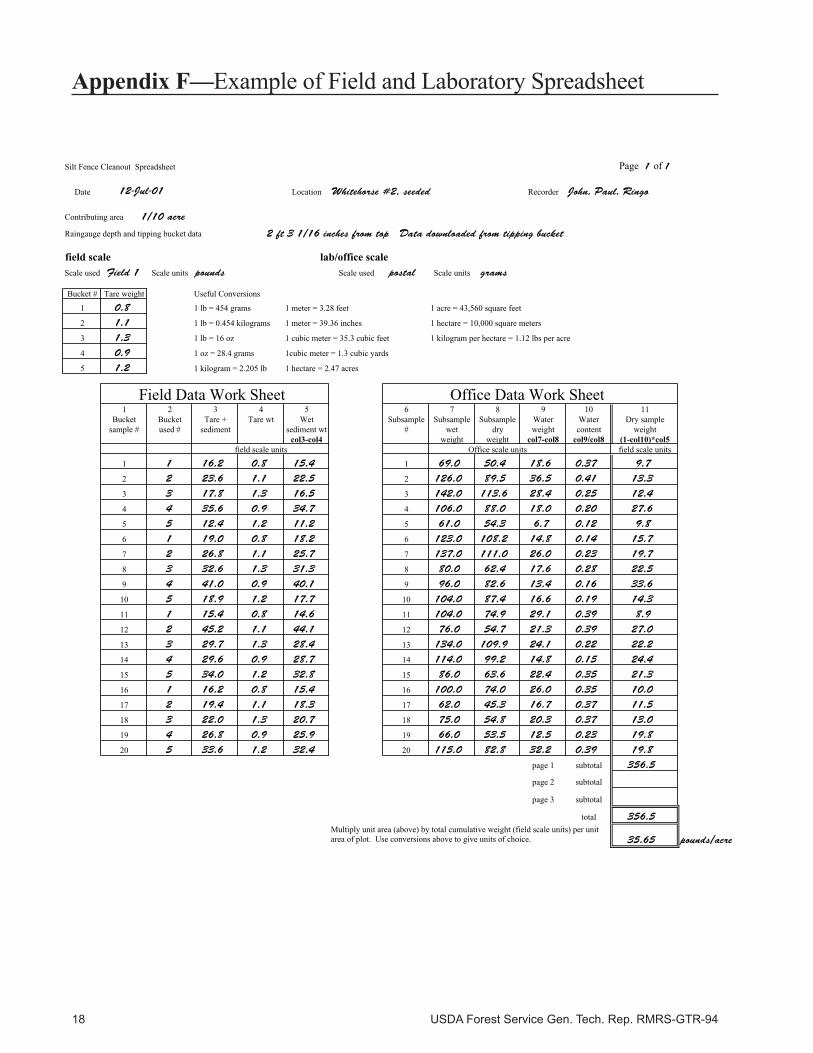
hours. Weigh the dry subsample and calculate gravi-
metric water content as shown in appendix F. If addi-
tional nutrient, organic matter, or particle size infor-
mation on the sediment is desired, take additional
subsamples for later processing.
Additional Data Collection
Precipitation Measurements
Precipitation collection methods can vary from ex-
pensive to low cost. Only low-cost methods will be
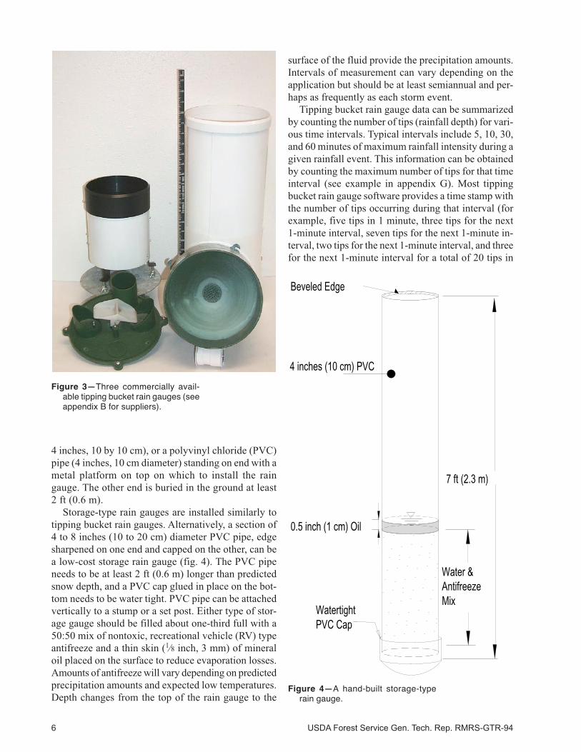
discussed in this paper. A tipping bucket rain gauge
provides information on the rainfall intensity and
amount (fig. 3). A storage-type rain gauge provides
cumulative precipitation only. For snow zone applica-
tion, an antifreeze-filled siphon attachment can be
added to the top of a tipping bucket rain gauge. Anti-
freeze can also be added to the storage-type rain gauge.
The antifreeze will melt the snow and provide the snow
water equivalent. Windscreens or windshields are ap-
propriate for open areas to aid in an accurate catch of
precipitation. In forested areas they are generally not
needed because the horizontal wind component is sub-
dued due to standing timber. Rain gauges are installed
near the silt fence erosion plots (less than 500 ft, 160 m
away) so they will be above estimated winter snow-
pack depth and not directly under tree canopy.
Tipping bucket rain gauges with a data pod (data
logger) became available in 2001 for under $300 and
provide excellent records of the rainfall intensity, event
amount, and time of the event (fig. 3). Commercial
software included with the rain gauge makes down-
loading and displaying this information easy. Tipping
bucket rain gauges are usually installed on a stump,
metal pole (1 inch, 2.5 cm diameter), wooden post (4 by
6 USDA Forest Service Gen. Tech. Rep. RMRS-GTR-94
4 inches, 10 by 10 cm), or a polyvinyl chloride (PVC)
pipe (4 inches, 10 cm diameter) standing on end with a
metal platform on top on which to install the rain
gauge. The other end is buried in the ground at least
2 ft (0.6 m).
Storage-type rain gauges are installed similarly to
tipping bucket rain gauges. Alternatively, a section of
4 to 8 inches (10 to 20 cm) diameter PVC pipe, edge
sharpened on one end and capped on the other, can be
a low-cost storage rain gauge (fig. 4). The PVC pipe
needs to be at least 2 ft (0.6 m) longer than predicted
snow depth, and a PVC cap glued in place on the bot-
tom needs to be water tight. PVC pipe can be attached
vertically to a stump or a set post. Either type of stor-
age gauge should be filled about one-third full with a
50:50 mix of nontoxic, recreational vehicle (RV) type
antifreeze and a thin skin (1⁄8 inch, 3 mm) of mineral
oil placed on the surface to reduce evaporation losses.
Amounts of antifreeze will vary depending on predicted
precipitation amounts and expected low temperatures.
Depth changes from the top of the rain gauge to the
surface of the fluid provide the precipitation amounts.
Intervals of measurement can vary depending on the
application but should be at least semiannual and per-
haps as frequently as each storm event.
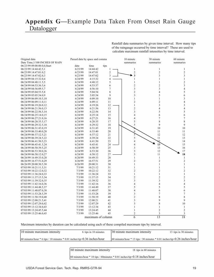
Tipping bucket rain gauge data can be summarized
by counting the number of tips (rainfall depth) for vari-
ous time intervals. Typical intervals include 5, 10, 30,
and 60 minutes of maximum rainfall intensity during a
given rainfall event. This information can be obtained
by counting the maximum number of tips for that time
interval (see example in appendix G). Most tipping
bucket rain gauge software provides a time stamp with
the number of tips occurring during that interval (for
example, five tips in 1 minute, three tips for the next
1-minute interval, seven tips for the next 1-minute in-
terval, two tips for the next 1-minute interval, and three
for the next 1-minute interval for a total of 20 tips in
Figure 3—Three commercially avail-able tipping bucket rain gauges (seeappendix B for suppliers).
Figure 4—A hand-built storage-typerain gauge.
Beveled Edge
4 inches (10 cm) PVC
0.5 inch (1 cm) Oil
7 ft (2.3 m)
WatertightPVC Cap
Water & AntifreezeMix
USDA Forest Service Gen. Tech. Rep. RMRS-GTR-94 7
5-minute interval). The maximum intensity is calculated
by adding the number of tips for the desired interval con-
verting the tips to depth of rainfall (inches or mm).
Ground Cover Measurements
Exposed bare soil on the hillslope is the most im-
portant soil factor affecting erosion rates. It is impor-
tant to measure bare soil exposed or conversely ground
cover, especially if the study is addressing vegetation
recovery or seeding effectiveness. Bare soil exposed
and ground cover can be measured with various tech-
niques. Chambers and Brown (1983) described these
techniques in detail. Ocular measurements are esti-
mated directly or divided into percentage classes (0 to
15, 15 to 30, 30 to 50, 50 to 70, 70 to 90, greater than
90 percent) of the area of interest, such as 1/100th acre
(0.004 ha) subplots.
Gridded metal or wooden frames are used for the
point-quadrant method. They usually have intersect-
ing lines (string or twine) at 4 to 6 inches (10 to 15 cm)
intervals for a 10 ft2 (1 m2) area (thus, for a 4 by 4 inch
grid in a 3 by 3 ft frame, there are 64 intersecting lines
excluding the frame). The frame is randomly located
(three to seven times) within the contributing area of
interest. The corners of the frame can be marked with
wood stakes or re-bar so the frame can be placed in the
same location during subsequent measurements. Al-
ternatively, the line-intercept method can be used.
However, this technique is generally used for larger
areas. Typical ground cover classes include bare soil, lit-
ter, duff, gravel, rock, live vegetation, stumps, and logs.
Data Analysis andInterpretation:
Statistical Design
Achieving a sound statistical design for silt fence
erosion plots is difficult due to high variability. Nearing
and others (1999) concluded that variability in erosion
plot data increases as the magnitude of the soil loss
increases. Thus, a few large events make comparison
between treatments difficult.
The number of replications needed to detect signifi-
cant differences in treatment effects depends on sev-
eral factors, including the inherent variability of the
site; natural variability (that is, microtopography,
microscale burn severity differences, root holes, soil
texture, rock content, and so forth); the allowable type
I error (usually a = 0.05 or a = 0.10); the probability
of accepting a false hypothesis, known as power of the
test and denoted by 1 - b; the magnitude of differences
to be detected; and the distribution of the data (normal
distribution). Most common analyses begin by
assuming normally distributed data. For silt fence ero-
sion data, this is generally not a reasonable assumption
for two reasons: first the data are often highly skewed
to the right (a few large events); secondly, there may
be many zeroes (rain events that did not produce any
sediment). Such departures from normality suggest log
transformation of the data before analysis. Alterna-
tively, nonparametric procedures, for nonnormal data
distributions, may be more appropriate for testing the
equality of medians (middle value of the data), rather
than the more usual t-test or analysis of variance for
means, (see appendix H).
If there are few zeros, departures from normality
may be helped by log transformation of the data be-
fore analysis. A better choice may be nonparametric
procedures, more appropriate for testing the equality
of median (middle value of the data), rather than more
familiar t-test or analysis of variance of means. An eas-
ily implemented nonparametric analysis for silt fence
erosion data is the Kruskal-Wallis rank sum test
(equivalent to a one-way analysis of variance on the
ranks of the original data) (Ott 1988; Walpole and
Myers 1985). This tests the equality of medians for
several treatments.
Most erosion scientists use five to seven replications
for erosion plot studies. Nearing and others (1999) sug-
gest comparing only treatments that will have large
differences in soil loss because small differences would
require too many replications to be practical. They sug-
gest five replications per treatment as a minimum. If
comparing two treatments, then nine replications per
treatment would be needed. The number of replica-
tions is based on the expected magnitudes of the mean
differences between treatments as well as the underly-
ing variability (measured by the variance) for the par-
ticular sites, soils, and treatments under consideration.
We have developed suggestions for various scenarios
that may be of interest assuming similar landscape,
soils, elevation, slope, and topography. Generally, silt
fences will be monitored for 2 to 3 years, thus changes
in erosion rates over time can also be detected.
Scenario 1—Timber Harvesting Effects: To de-
termine erosion amounts for various activities within
a timber sales unit, identify the various activities (treat-
ments) that occur within the sale boundary. These could
include log-landing areas, haul road, repeatedly used
skid trail, few pass skid trail, and control (undisturbed)
areas. One would need to reduce the number of treat-
ments to two and a control to be able to make a reason-
able statistical design. For example, nine silt fences on

8 USDA Forest Service Gen. Tech. Rep. RMRS-GTR-94
the haul road; nine silt fences on the repeatedly used
skid trail, and the remaining nine silt fences for the
control. The total of 27 silt fences would be moni-
tored for 3 years.
Scenario 2—Testing Seeding Mixes Post Wildfire:
To determine erosion rates for two seeding mixes (seed
mix A and seed mix B) and a control (no seeding)
after a wildfire. In this scenario, ground cover would
also need to be measured (described in the “Additional
Data Collection” section). Thus, nine replications of
each treatment would be needed. The total of 27 silt
fences would be monitored for 3 years.
Scenario 3—Comparing Prescribed Fire or Wild-
fire Erosion Rates: To determine erosion amounts
from a prescribe fire or wildfire and a control (no fire).
Thus, five replications of each treatment would be
needed. This total of 10 silt fences would be moni-
tored for 2 years.
Silt fence data can be organized and analyzed using
a computer spreadsheet (appendix F). Calculate the
sediment amounts for each collection period and con-
vert to weight per area. Determine rainfall amounts and
rainfall intensity for that collection period. Compare
sediment yields with rainfall amounts and/or intensity,
remembering that rainfall can vary over short distances.
Variability in the data is to be expected; there are in-
herent variations in soils, below ground organic mat-
ter, and so forth, that can influence sediment output.
That variability, combined with the effects of the treat-
ment, can make interpreting the results challenging. If
a statistically designed layout was used then it will be
easier to develop and run a statistically valid analysis.
Each collection period may be a “repeated measure”
for the same silt fence during the study period.
Summary
Silt fences are an economical method to obtain
hillslope erosion measurements. They can be installed
with a small field crew and maintained at various
time intervals, depending on the storm production
accuracy of the information that is desired. When
installed and maintained properly, they can trap and
store sediment until it is cleaned out and measured.
Erosion measurements from silt fences can be used
to validate model estimates, demonstrate treatment
or management practice effects, and compare seed-
ing treatments on hillslope erosion.
ReferencesASTM. 1995. D 4751-95 Standard Test Method for determining
apparent opening size of a geotextile. Annual book of ASTMstandards, Vol. 4.09. West Conshohocken, PA: ASTM: 983–987.
ASTM. 1996. D 4491-96 Standard Test Methods for waterpermeability of geotextiles by permittivity. Annual book ofASTM standards, Vol. 04.09. West Conshohocken, PA: ASTM:945–950.
Britton, Sherry L.; Robinson, Kerry M.; Barfield, Billy J.; Kadavy,K. C. 2000. Silt fence performance testing. Presented at: Annualmeeting of the American Society of Agricultural Engineers;2000 July. Paper 002162. St. Joseph, MI: American Society ofAgricultural Engineers. 11 p.
Britton, Sherry L.; Robinson, Kerry M.; Barfield, Billy J. 2001.Modeling the effectiveness of silt fence. In: Proceedings:Seventh Federal Interagency Sedimentation Conference; 2001March 25-29; Reno, NV. Vol. 2. U.S. Department of Agriculture,Natural Resources Conservation Service: V/75–82.
Carpenter, Thomas. 1999. Silt fence that works for designers,installers, inspectors. In: Carpenter Erosion Control. SteamboatSprings, CO: International Erosion Control Association. 56 p.
Chambers, Jeanne C.; Brown, Ray W. 1983. Methods forvegetation sampling and analysis on revegetated mined lands.Gen. Tech. Rep. INT-151. Ogden, UT: U.S. Department ofAgriculture, Forest Service, Intermountain Forest and RangeExperiment Station. 57 p.
Conover, W. J. 1971. Practical nonparametric statistics. New York:John Wiley & Sons, Inc. 962 p.
Conover, W. J.; Iman, Ronald. 1981. Rank transformation as abridge between parametric and nonparametric statistics. TheAmerican Statistician. 35: 124–133.
Dissmeyer, G. E. 1982. How to use fabric dams to compare erosionfrom forestry practices. Forestry Rep. SA-FR 13. Atlanta, GA:U.S. Department of Agriculture, Forest Service, SoutheastAreas. 11 p.
Dissmeyer, G. E.; Foster, G. R. 1980. A guide for predicting sheetand rill erosion on forest lands. Tech. Publ. SA-TP 11. Atlanta,GA: U.S. Department of Agriculture, Forest Service, SoutheastAreas. 40 p.
Foster, G. R. 1982. Modeling the erosion process. In: Haan, C. T.;Johnson, H. P.; Brakensiek, D. L., eds. Hydrologic modelingof small watersheds. St. Joseph, MI: American Society ofAgricultural Engineers: chapter 8.
Hahn, Gerald J.; Meeker, William Q. 1991. Statistical intervals: aguide for practitioners. New York: John Wiley & Sons, Inc.416 p.
Jiang, Naiqian; Hirschi, Michael C.; Cooke, Richard A. C.;Mitchell, J. Kent. 1996. Equation for flow through filterfabric. Presented at: Annual meeting of the American Societyof Agricultural Engineers; 1996 July. Paper 962098. St.Joseph, MI: American Society of Agricultural Engineers.14 p.
McNabb, David H.; Swanson, Frederick J. 1990. Effects of fireon soil erosion. In: Natural and prescribed fire in PacificNorthwest forests. Walstad, John D.; [and others], eds.Corvallis: Oregon State University Press: 159–176.
Megahan, Walter F.; Seyedbagheri, Kathleen A.; Mosko, Timothy L.;Ketcheson, Gary L. 1986. Construction phase sediment budgetfor forest roads on granitic slopes in Idaho. In: Hadley, RichardF., ed. Drainage basin sediment delivery, proceedings; 1986;Albuquerque, NM. IAHS Publ. 159. Wallingford, Oxon, UK:31–39.
Nearing, Mark A.; Gover, Gerard; Norton, L. Darrell. 1999.Variability in soil erosion data from replicated plots. SoilScience Society of America Journal. 63: 1829–1835.
Ott, Lyman. 1988. An introduction to statistical methods and dataanalysis. 3d ed. Boston, MA: PWS-Kent Publishing Co. 835 p.
Robichaud, P. R.; McCool, D. K.; Pannkuk, C. D.; Brown, R. E.;Mutch, P. W. 2001. Trap efficiency of silt fences used in hillslopeerosion studies. In: Ascough, J. C., II; Flanagan, D. C., eds. Soilerosion research for the 21st century, proceedings; 2001;Honolulu, HI. St. Joseph, MI: American Society of AgriculturalEngineers: 541–543.

USDA Forest Service Gen. Tech. Rep. RMRS-GTR-94 9
Trow Consulting Engineers Ltd. 1996. Instream sediment controltechniques field implementation manual. FG-007. SouthPorcupine, Ontario (Canada): Ministry of Natural Resources,Northeast Science and Technology. 109 p.
Walpole, Ronald E.; Myers, Raymond H. 1985. Probability andstatistics for engineers and scientists. 3d ed. New York:Macmillan Publishing Co. 639 p.
Wishowskie, J. M.; Mamo, M.; Bubenzer, G. D. 1998. Trapefficiencies of filter fabric fence. Presented at: Annual meetingAmerican Society of Agricultural Engineers; 1998 July. Paper982158. St. Joseph, MI: American Society of AgriculturalEngineers. 14 p.
Wyant, D. C. 1980. Evaluation of filter fabrics for use as silt fences.VHTRC 80-R49. Charlottesville: Virginia Highway andTransportation Research Council.
10 USDA Forest Service Gen. Tech. Rep. RMRS-GTR-94
Appendix A—Volume of Silt Fence Storage Capacity For VariousConfigurations of Ground Surface Slope, Silt Fence Height, andWidth
Silt fence maximum holding capacities (ft3)Silt fence Ground surface slope
(%)Height Width
ft ft 5 10 15 20 25 30 35 40 45 50 55 60 65 70
1.5 10 177 88 59 44 35 29 25 22 20 18 16 15 14 131.5 20 353 177 118 88 71 59 50 44 39 35 32 29 27 251.5 30 530 265 177 133 106 88 76 66 59 53 48 44 41 381.5 40 707 353 236 177 141 118 101 88 79 71 64 59 54 501.5 50 884 442 295 221 177 147 126 110 98 88 80 74 68 632.0 10 314 157 105 79 63 52 45 39 35 31 29 26 24 222.0 20 628 314 209 157 126 105 90 79 70 63 57 52 48 452.0 30 942 471 314 236 188 157 135 118 105 94 86 79 72 672.0 40 1,257 628 419 314 251 209 180 157 140 126 114 105 97 902.0 50 1,571 785 524 393 314 262 224 196 175 157 143 131 121 1122.5 10 491 245 164 123 98 82 70 61 55 49 45 41 38 352.5 20 982 491 327 245 196 164 140 123 109 98 89 82 76 702.5 30 1,473 736 491 368 295 245 210 184 164 147 134 123 113 1052.5 40 1,963 982 654 491 393 327 280 245 218 196 178 164 151 1402.5 50 2,454 1,227 818 614 491 409 351 307 273 245 223 205 189 175
Silt fence maximum holding capacities (m3)Silt fence Ground surface slope
(%)Height Width
(m) (m) 5 10 15 20 25 30 35 40 45 50 55 60 65 70
0.45 3 5 2 2 1 1 1 1 1 1 0.5 0.5 0.5 0.5 0.5.45 6 10 5 3 2 2 2 1 1 1 1 1 1 1 1.45 9 14 7 5 4 3 2 2 2 2 1 1 1 1 1.45 12 19 10 6 5 4 3 3 2 2 2 2 2 1 1.45 15 24 12 8 6 5 4 3 3 3 2 2 2 2 2.60 3 8 4 3 2 2 1 1 1 1 1 1 1 1 1.60 6 17 8 6 4 3 3 2 2 2 2 2 1 1 1.60 9 25 13 8 6 5 4 4 3 3 3 2 2 2 2.60 12 34 17 11 8 7 6 5 4 4 3 3 3 3 2.60 15 42 21 14 11 8 7 6 5 5 4 4 4 3 3.75 3 13 7 4 3 3 2 2 2 1 1 1 1 1 1.75 6 27 13 9 7 5 4 4 3 3 3 2 2 2 2.75 9 40 20 13 10 8 7 6 5 4 4 4 3 3 3.75 12 53 27 18 13 11 9 8 7 6 5 5 4 4 4.75 15 66 33 22 17 13 11 9 8 7 7 6 6 5 5

USDA Forest Service Gen. Tech. Rep. RMRS-GTR-94 11
The following terms are used for silt fence specifi-
cations related to the trap efficiency (ASTM 1995,
1996). Table B1 provides specifications for various silt
fences. These silt fences should perform well for most
soil conditions. Generally, lower permittivity valued
silt fences will trap more sediment but water flow rates
are also reduced.
Permittivity
Permittivity of geotextiles is a measurement of the
amount of water per unit cross-sectional area per unit
head that flows through the geotextile, without any
extra force on the water (laminar flow conditions). It
is an indicator of the quantity of water that can pass
through a geotextile in an isolated condition. Because
there are geotextiles of various thickness, evaluation
in terms of the permeability can be misleading. It is
more significant to evaluate the quantity of water that
will flow through the material under a given head over
a particular area; this is expressed as permittivity. The
units of permittivity are sec-1. This is derived from the
formula for permittivity:
Permittivity = Q/(h*A*t)
Where Q is the quantity of water flow through silt fence
fabric (inch3, mm3), h is the head of water on the silt
fence (inch, mm), A is the cross-sectional area (inch2,
mm2), and t is the time for flow, Q, (sec).
Water Flow Rate
The Water Flow Rate of a geotextile is a measure-
ment of the volume of water that will pass through the
Appendix B—Common Silt Fence Specifications
material per unit time per unit area. The units are (com-
monly) gal min-1 ft-2 (L min-1 m-2). Unlike permittiv-
ity, this value will be affected by thickness of the fab-
ric and other factors such as apparent opening size
(AOS).
Apparent Opening Size (AOS)
The AOS of a geotextile is a property that approxi-
mates the largest particle that will effectively pass
through the fabric. It is figured by using the geotextile
as a filter and sifting various (standardized) sizes of
glass beads through the material. This is an important
characteristic when designing silt fences because it is
crucial that the AOS be small enough that it will hold
back nearly all of the sediment, while at the same time
not clog easily and allow water to pass through. The
AOS is measured in a standard U.S. Sieve number (20
to 80) with 20 being a large opening and 80 being small.
Equivalent values include:
Sieve number equivalencies
Sieve Opening size
no. inch mm
20 0.033 0.840
30 .023 .590
40 .017 .420
50 .012 .297
60 .010 .250
70 .008 .210
80 .007 .177

12 USDA Forest Service Gen. Tech. Rep. RMRS-GTR-94
Manufactor and Permittivity
Product Design (sec-1) (gal min -1 ft -2) (L min -1 m -2) (US Sieve) (mm)
Agri Drain
Biotech 760 0.45 30 1225 20 0.850
NILEX
2130 (Amoco Fabric) 0.05 10 405 30 0.600
910 (SI Industries) 0.20 15 610 20 0.850
915 (SI Industries) 0.40 25 1020 40 0.425
Amoco
Style 2130 0.05 10 405 30 0.600
Exxon
GTF 100S NA 125 5095 50-70 .40-.20
ADS
ADS 3302WP / 3302WT 0.01 50 2035 20 0.840
TC Mirafi
Silt Fence 0.10 10 405 30 0.600
(stakes attached)
100X 0.10 10 405 30 0.600
LINQ Indust. Fabrics
GTF 170 0.05 20 815 20 0.850
GTF 180 0.05 7 285 20 0.850
(GTF 170 and 180 differ in strength)
GTF 190 0.07 12 490 30 0.600
GTF 200S 0.07 12 490 50 0.300
Belton Industries (available in 3 different colors)
751 / 894 / 897 0.10 15 610 30 0.600
(dimensions differ)
755 / 890 NA 25 1020 30 0.600
(dimensions differ)
806 / 810 0.20 20 815 20 0.850
(dimensions differ)
DGI Industries
P - Series 0.10 10 405 30 0.600
BIG R
(Mutual Industries Fabric)
Mutual MISF180 NA 30 1225 40 0.425
Typical
Burst Strength 160-400 Psi (100-2760 Kpa)
Puncture Strength 25-90 lbs (0.11-0.40 kN)
Tensile Strength 80-180 lbs (0.35-0.80 kN)
Water Flow Rate AOS
Table B1—Specifications related to trap efficiency of silt fences. Typical strength characteristics are also provided.

USDA Forest Service Gen. Tech. Rep. RMRS-GTR-94 13
This list of products and businesses is provided as
an information tool only and does not imply endorse-
ment by the Forest Service or the U.S. Department of
Agriculture. All listed prices were as of 2002.
Silt Fence Distributors
ACF Environmental (Amoco Fabrics)
2831 Cardwell Road
Richmond, VA 23234
Toll free: 1-800-448-3636
Web: www.acfenvironmental.com
Big R Manufacturing & Distributing (Mutual Indus-
tries Distributor)
P.O. Box 1290
Greeley, CO 80632-1290
Toll free: 1-800-234-0734
Fax: (970) 356-9621
Web: www.bigrmfg.com/construc.htm
Cobb Lumber Co. (LINQ Industrial Fabrics Distributor)
P.O. Box 808
Timpson, TX 75975
Toll free: 1-888-322-2622
Fax: (936) 254-2763
Web: www.cobblumber.com
Liberty Equipment Co. (Belton Industries Distributor)
10879 Houser Drive
Fredericksburg, VA 22408
Tel: (540) 898-8933
Fax: (540) 898-8650
Web: www.libertyequipment.com
Nilex Corp. (Amoco & SI Fabrics with custom stakes)
15171 E. Fremont Drive
Englewood, CO 80112
Tel: (303) 766-2000
Edmonton (780) 463-9535
Calgary (403) 543-5454
Vancouver (604) 420-6433
Winnipeg (204) 925-4466
Web: www.nilex.com
Silt Fence Manufacturers
Advanced Drainage Systems, Inc. a
3300 Riverside Drive
Columbus, OH 43221
Tel: (614) 457-3051
Fax: (614) 538-5204
Web: www.ads-pipe.com
Agri Drain Co. a
Toll Free: 1-800-232-4742
Fax: 1-800-282-3353
Web: www.agridrain.com
Belton Industries, Inc. a
8613 Roswell Rd.
Atlanta, GA 30350
Tel: (770) 587-0257
Toll Free: 1-800-225-4099
Fax: (770) 992-6361
Toll Free: 1-800-851-4029
E-mail: [email protected]
Web: www.beltonindustries.com
DGI Industries a
P.O. Box 70
Bennington, NH 03442
Tel: (603) 641-2850
Toll Free: 1-888-745-8344
Fax: (603) 669-6991 (24 hour)
Web: www.dgiindustries.com
Exxon Chemical Americas
2100 River Edge Parkway, Suite 1025
Atlanta, GA 30328-4654
Toll Free: 1-800-543-9966
LINQ Industrial Fabrics, Inc.
2550 West Fifth North Street
Somerville, SC 29483-9699
Tel: (843) 873-5800
Toll Free: 1-800-445-4675
Fax: (843) 875-8111
E-mail: [email protected]
Web: www.linqind.com
Appendix C—List of Suppliers for Silt Fences and Rain Gauges

14 USDA Forest Service Gen. Tech. Rep. RMRS-GTR-94
Mutual Industries, Inc. a
707 W. Grange St.
Philadelphia, PA 19120
Tel: (215) 927-6000
Toll Free: 1-800-523-0888
Fax: (215) 927-8888
E-mail: [email protected]
Web: www.mutualindustries.com
SI Geosolutions
6025 Lee Highway, Suite 435
Chattanooga, TN 37421
Toll Free: 1-800-621-0444
Fax: (423) 899-7619
Web: www.fixsoil.com
Database of representatives on Web site
TC Mirafi
Lake Forest, CA
Tel: (949) 859-2850
Web: www.tcmirafi.com
Database of representatives/distributors on Web site
Note: Many of the companies listed sell silt fences with
stakes preattached, sometimes at buyer’s specified in-
tervals; otherwise they are generally 4 to 10 ft (1.2 to 3 m)
apart. Additional stakes can easily be added between
the preattached stakes.
Local lumberyards or building suppliers may have
silt fence fabric or can obtain it.a Sells factory direct.
Rain Gauges
Onset Computer Corp.
P.O. Box 3450
Pocasset, MA 02559-3450
Tel: (508) 759-9500
Toll Free: 1-800-564-4377
Fax: (508) 759-9100
E-mail: [email protected]
Web: www.onsetcomp.com (Online ordering available)
Data Logging Rain Gauge Model RG2 (English ver-
sion) and RG2-M (metric version) are fully self-con-
tained, battery-powered rainfall data collection and
recording systems. They include a HOBO Event data
logger integrated into a tipping-bucket rain gauge. The
RG2 automatically records up to 80 inches (160 cm
for the RG2-M) of rainfall data that can be used to
determine rainfall rates, times, and duration. A time
and date stamp is stored for each 0.01 inches (0.2 mm
for the RG2-M) tip event for detailed analysis. Price:
$380 (2002). HOBO Event Logger Price: $85 (2002)
(can be attached to RainWise Rain Gauge, as well as
Davis Instruments Rain Collector).
Required Software: Boxcar Pro or Boxcar 3.0+
starter kits include software, PC interface cable and
manual. Price: Boxcar Pro 4.0 Windows Starter Kit $95
(2002), Boxcar 3.7 Windows Starter Kit $14 (2002).
Boxcar Pro for MAC OS free on Web site, Mac Inter-
face Cable $9 (2002).
RainWise Inc.
25 Federal Street
Bar Harbor, ME 04609
Tel: (207) 288-5169
Toll Free: 1-800-762-5723
Fax: (207) 288-3477
E-mail: [email protected]
Web: www.rainwise.com (Online ordering available)
RainWise provides a large selection of rain gauges
and data loggers that can be purchased as a single unit
or bought separately then assembled. They are capable
of recording 0.01 inch of rainfall as well as putting a
time and date stamp at specified intervals during an
event. Total System (rain gauge and built-in logger):
Rain Logger Price: $295 (2002), Tipping Bucket Rain
Gauge (wired) Price: $69.95 (2002), Data Logger Price:
$120 (2002).
A PC interface cable and necessary software is in-
cluded with the Rain Logger and the information can
easily be exported into a spreadsheet for graphing and
other data analysis. Also, software is available for
download from the RainWise Web site.
Spectrum
23839 W. Andrew Rd.
Plainfield, IL 60544
Tel: (815) 436-4440
Toll Free: 1-800-248-8873
Fax: (815) 436-4460
E-mail: [email protected]
Web: www.specmeters.com (Online ordering available)
Spectrum’s Data Logging Rain Gauge provides high
accuracy with a low-maintenance tipping bucket de-
sign. The logger records accumulated rainfall during
each interval, maximum of 2.55 inches per interval.
User selected intervals are 1, 5, 10, 15, 30, 60, and 120
minutes. Logger capacity is 7,000 intervals.
Use with SpecWare 6 Software for analysis and re-
porting. WatchDog rain collectors and SpecWare
Software can be programmed to record rainfall in

USDA Forest Service Gen. Tech. Rep. RMRS-GTR-94 15
either English (inches) or metric (mm) units. The rain
gauge and data logger may also be purchased sepa-
rately and assembled.
Total System (gauge and built-in logger): Data Log-
ging Rain Gauge Price: $199 (2002), Digital Tipping
Bucket Rain Gauge Price: $74.95 (2002), WatchDog-
115 Rain Logger Price: $85 (2002).
Required Software: Specware 6.0 Software (includes
PC interface cable) Price: $99.
Davis Instruments
4701 Mount Hope Drive
Baltimore, MD 21215
Tel: (410) 358-3900
Toll Free: 1-800-988-4895
Fax: (410) 358-0252
Toll Free Fax: 1-800-433-9971
E-mail: [email protected]
Web: www.davis.com
The Rain Collector II measures rainfall in 0.01 inch
increments in the English version and 0.2 mm in the
metric version. Can be outfitted with data logger (see
Onset Inc. for HOBO even logger). Davis Rain Col-
lector II-English or Metric Rain Collector II Price: $75
(2002).
Ben Meadows Company (Distributor)
Subsidiary of Lab Safety Supply Inc.
P.O. Box 5277
Janesville, WI 53547-5277
Tel: (608) 743-8001
Toll Free: 1-800-241-6401
Toll Free Fax: 1-800-628-2068
E-mail: [email protected]
Web: www.benmeadows.com (Online ordering avail-
able)
Ben Meadows is a distributor of different rain gauges
and weather monitoring equipment. The Onset Data
Logging Rain Gauge, the Rainwise Tipping Bucket
Rain Gauge, the Davis Rain Collector, and the Onset
HOBO Event Logger are available.

16 USDA Forest Service Gen. Tech. Rep. RMRS-GTR-94
Silt Fence Installation Tools
• Shovels (square and round nosed type)
• Pulaski
• Hand trowels
• Claw hammer
• Sledgehammer
• Heavy-duty stapler
• Flagging
• Pin flags
• Measuring tape
• Steel cap for driving wooden stakes
• Caulking gun
Silt Fence Installation Supplies
• Wooden stake (2 by 2 inches by 4 ft, 5 by 5 cm by
1.2 m)
• Silt fence fabric (100 ft by 36 inches or 42 inches,
30 m by 0.9 or 1.1 m) rolls, 42 inch width preferred
• Staples (0.5 inch, 1 cm), or roofing nails (1 inch,
2.5 cm) with plastic washers, or 16-gauge wire or
plastic zip ties (10 inches, 25 cm)
• Tar paper strips or plastic strips
• Red construction chalk (1 gal, 4 l)
• Construction adhesive or silicon
Sediment Cleanout Tools
• Hanging or platform scale (fish scale: capacity 50 lb
with 1-lb increment, 22 kg with 0.2-kg)
• Shovel (square nosed)
• Hand brush or broom
• Hand trowel (it is best to round-over sharp corners
and points with file or grinder, so it does not catch
the fabric)
• Notebook/data sheets (waterproof) and pencils
• Red construction chalk (1 gal, 4 l)
• Tripod or tree branch or metal angle tied to tree for
hanging scale
• Extra silt fence fabric (for repairs)
• Plastic wire ties (100)
• Construction adhesive or silicon caulk
• 4 plastic buckets (5 gal, 19 l)
Appendix D—Equipment List
Figure D1—Steel cap for poundingwooden stakes into the ground.

USDA Forest Service Gen. Tech. Rep. RMRS-GTR-94 17
Appendix E—Example of Field Data Sheet
Silt Fence Cleanout Field Datasheet Page of
Date Location Recorder
Contributing areaRaingauge depth and tipping bucket data
field scaleScale used Scale units
Bucket # Tare weight
12345
Bucketsample #
Tare wt
sed wtcol3-col4
1
2
3
4
5
6
7
8
9
10
11
12
13
14
15
16
17
18
19
20
Remarks: Include repairs needed and made. Supplies needed for next visit.
field scale units
Whitehorse #2, seeded John, Paul, Ringo
1 1
12-Jul-01
1/10 acre
2 ft 3 1/16 inches from top
Field 1 pounds
Data downloaded from tipping bucket
0.8
1.1
1.3
0.91.2
1
2
3
4
5
1
2
3
4
5
1
2
3
4
5
1
2
3
4
5
1 2 3 4 5
Bucketused #
Tare +sediment
WetSubsample
taken?
Need to bring more antifreeze and new dessicant. Shovel handle broke, need new shovel.
Still have small amount of snow in upper watershed. Rain guage had needles and dust accumulation.
16.2
23.6
17.8
35.6
12.4
19.0
26.8
32.6
41.0
18.9
15.4
45.2
29.7
29.6
34.0
16.2
19.4
22.0
26.8
33.6
0.8
1.1
1.3
0.9
1.2
0.8
1.1
1.3
0.9
1.2
0.8
1.1
1.3
0.9
1.2
0.8
1.1
1.3
0.9
1.2
15.4
22.5
16.5
34.7
11.2
18.2
25.7
31.3
40.1
17.7
14.6
44.1
28.4
28.7
32.8
15.4
18.3
20.7
25.9
32.4
18 USDA Forest Service Gen. Tech. Rep. RMRS-GTR-94
Appendix F—Example of Field and Laboratory Spreadsheet
Silt Fence Cleanout Spreadsheet Page 1 of 1
Date Location Whitehorse #2, seeded Recorder John, Paul, Ringo
Contributing area 1/10 acre
Raingauge depth and tipping bucket data
field scale lab/office scaleScale used Field 1 Scale units pounds Scale used postal Scale units grams
Bucket # Tare weight Useful Conversions
1 0.8 1 lb = 454 grams 1 meter = 3.28 feet 1 acre = 43,560 square feet
2 1.1 1 lb = 0.454 kilograms 1 meter = 39.36 inches 1 hectare = 10,000 square meters
3 1.3 1 lb = 16 oz 1 cubic meter = 35.3 cubic feet 1 kilogram per hectare = 1.12 lbs per acre
4 0.9 1 oz = 28.4 grams 1cubic meter = 1.3 cubic yards
5 1.2 1 kilogram = 2.205 lb 1 hectare = 2.47 acres
1 2 3 4 5 6 7 8 9 10 11Bucket Bucket Tare + Tare wt Wet Subsample Subsample Subsample Water Water Dry sample
sample # used # sediment sediment wt # wet dry weight content weightcol3-col4 weight weight col7-col8 col9/col8 (1-col10)*col5
field scale units
1 1 16.2 0.8 15.4 1 69.0 50.4 18.6 0.37 9.7
2 2 23.6 1.1 22.5 2 126.0 89.5 36.5 0.41 13.3
3 3 17.8 1.3 16.5 3 142.0 113.6 28.4 0.25 12.4
4 4 35.6 0.9 34.7 4 106.0 88.0 18.0 0.20 27.6
5 5 12.4 1.2 11.2 5 61.0 54.3 6.7 0.12 9.8
6 1 19.0 0.8 18.2 6 123.0 108.2 14.8 0.14 15.7
7 2 26.8 1.1 25.7 7 137.0 111.0 26.0 0.23 19.7
8 3 32.6 1.3 31.3 8 80.0 62.4 17.6 0.28 22.5
9 4 41.0 0.9 40.1 9 96.0 82.6 13.4 0.16 33.6
10 5 18.9 1.2 17.7 10 104.0 87.4 16.6 0.19 14.3
11 1 15.4 0.8 14.6 11 104.0 74.9 29.1 0.39 8.9
12 2 45.2 1.1 44.1 12 76.0 54.7 21.3 0.39 27.0
13 3 29.7 1.3 28.4 13 134.0 109.9 24.1 0.22 22.2
14 4 29.6 0.9 28.7 14 114.0 99.2 14.8 0.15 24.4
15 5 34.0 1.2 32.8 15 86.0 63.6 22.4 0.35 21.3
16 1 16.2 0.8 15.4 16 100.0 74.0 26.0 0.35 10.0
17 2 19.4 1.1 18.3 17 62.0 45.3 16.7 0.37 11.5
18 3 22.0 1.3 20.7 18 75.0 54.8 20.3 0.37 13.0
19 4 26.8 0.9 25.9 19 66.0 53.5 12.5 0.23 19.8
20 5 33.6 1.2 32.4 20 115.0 82.8 32.2 0.39 19.8
page 1 subtotal 356.5
page 2 subtotal
page 3 subtotal
total 356.5
35.65 pounds/acreMultiply unit area (above) by total cumulative weight (field scale units) per unit area of plot. Use conversions above to give units of choice.
12-Jul-01
Field Data Work Sheet Office Data Work Sheet
field scale units Office scale units
2 ft 3 1/16 inches from top Data downloaded from tipping bucket
USDA Forest Service Gen. Tech. Rep. RMRS-GTR-94 19
Appendix G—Example Data Taken From Onset Rain GaugeDatalogger
Rainfall data summaries by given time interval. How many tips
of the raingauge occurred by time interval? These are used to calculate maximum rainfall intensities by time interval.
Original data Parsed data by space and comma 10 minute 30 minute 60 minute
Date Time,1/100 INCHES OF RAIN summaries summaries summaries
06/23/99 09:00:00.0,0,Start date time tips
06/23/99 14:44:42.5,1 6/23/99 14:44:42 1 1 1 1
06/23/99 14:47:01.0,2 6/23/99 14:47:01 2 2 2 2
06/23/99 14:47:02.0,3 6/23/99 14:47:02 3 3 3 3
06/24/99 04:15:32.0,4 6/24/99 4:15:32 4 1 1 1
06/24/99 04:48:11.5,5 6/24/99 4:48:12 5 1 1 2
06/24/99 04:53:36.5,6 6/24/99 4:53:37 6 2 2 3
06/24/99 04:56:09.5,7 6/24/99 4:56:10 7 3 3 4
06/24/99 05:04:53.5,8 6/24/99 5:04:54 8 2 4 5
06/24/99 05:05:54.0,9 6/24/99 5:05:54 9 3 5 6
06/24/99 06:09:10.5,10 6/24/99 6:09:10 10 1 1 3
06/24/99 06:09:11.0,11 6/24/99 6:09:11 11 2 2 4
06/24/99 06:19:26.0,12 6/24/99 6:19:26 12 1 3 3
06/24/99 06:21:56.0,13 6/24/99 6:21:56 13 2 4 4
06/24/99 06:22:56.5,14 6/24/99 6:22:56 14 3 5 5
06/24/99 06:25:14.0,15 6/24/99 6:25:14 15 4 6 6
06/24/99 06:27:21.0,16 6/24/99 6:27:21 16 4 7 7
06/24/99 06:28:35.5,17 6/24/99 6:28:35 17 5 8 8
06/24/99 06:29:32.5,18 6/24/99 6:29:32 18 5 9 9
06/24/99 06:31:43.0,19 6/24/99 6:31:43 19 6 10 10
06/24/99 06:33:40.0,20 6/24/99 6:33:40 20 6 11 11
06/24/99 06:37:12.5,21 6/24/99 6:37:12 21 5 12 12
06/24/99 06:39:24.5,22 6/24/99 6:39:24 22 5 11 13
06/24/99 06:41:50.5,23 6/24/99 6:41:50 23 4 12 14
06/24/99 06:45:41.5,24 6/24/99 6:45:41 24 4 13 15
06/24/99 06:50:39.5,25 6/24/99 6:50:39 25 3 13 16
06/24/99 06:53:30.0,26 6/24/99 6:53:30 26 3 12 17
06/24/99 06:58:12.0,27 6/24/99 6:58:12 27 3 11 18
06/26/99 16:49:33.0,28 6/26/99 16:49:33 28 1 1 1
06/26/99 16:57:51.0,29 6/26/99 16:57:51 29 2 2 2
06/26/99 20:00:30.5,30 6/26/99 20:00:31 30 1 1 1
07/03/99 10:21:11.5,31 7/3/99 10:21:12 31 1 1 1
07/03/99 10:22:12.0,32 7/3/99 10:22:12 32 2 2 2
07/03/99 11:36:24.0,33 7/3/99 11:36:24 33 1 1 1
07/03/99 11:37:15.5,34 7/3/99 11:37:15 34 2 2 2
07/03/99 11:39:32.0,35 7/3/99 11:39:32 35 3 3 3
07/03/99 11:42:16.0,36 7/3/99 11:42:16 36 4 4 4
07/03/99 11:44:48.5,37 7/3/99 11:44:49 37 5 5 5
07/03/99 11:48:07.0,38 7/3/99 11:48:07 38 4 6 6
07/03/99 11:53:28.5,39 7/3/99 11:53:28 39 3 7 7
07/03/99 11:58:19.0,40 7/3/99 11:58:19 40 2 8 8
07/03/99 12:00:21.5,41 7/3/99 12:00:21 41 3 9 9
07/03/99 12:07:29.0,42 7/3/99 12:07:29 42 3 8 10
07/03/99 13:12:34.0,43 7/3/99 13:12:34 43 1 1 1
07/03/99 13:24:45.5,44 7/3/99 13:24:45 44 1 2 2
07/03/99 13:25:46.0,45 7/3/99 13:25:46 45 2 3 3
maximum of column 6 13 18
Maximum intensites by duration can be calculated using each of these compiled maximum tips by interval.
10 minute maximum intensity 6 tips in 10 minutes 30 minute maximum intensity 13 tips in 30 minutes
60 minutes/hour * 6 tips / 10 minutes * 0.01 inches/tip=0.36 inches/hour 60 minutes/hour * 13 tips / 30 minutes * 0.01 inches/tip=0.26 inches/hour
60 minute maximum intensity 18 tips in 60 minutes
60 minutes/hour * 18 tips / 60minutes * 0.01 inches/tip=0.18 inches/hour

20 USDA Forest Service Gen. Tech. Rep. RMRS-GTR-94
Appendix H—Statistical Analysis Procedure
This section describes a simple approach to analyze
silt fence erosion data. Additional statistical analysis
can be performed on the data, but it may be necessary
to consult statistical textbooks or get statistical assis-
tance. This example should be viewed as a first ap-
proach for data analysis. The data represent five silt
fences for a Burn Only treatment, four silt fences for
Burn and Seed treatment, and three silt fences for the
Control (no burn) treatment. Fifteen storm events were
observed with some events producing no sediment.
Generally it is best to analyze data after 15 to 20 storm
events or a season.
A common occurrence with erosion or sediment
yield data is that the underlying distribution is not nor-
mal or gaussian. This is due to a large number of ze-
roes (when there was no runoff) together with a few
large values, indicating the underlying distribution is
skewed to the right. For highly skewed data, the usual
normality assumption is violated, and, consequently,
the “usual” confidence intervals, t-tests, and analysis
of variance procedures may not be appropriate. Instead,
less restrictive nonparametric procedures should be
used.
As with any data set, one should first explore the
data to determine whether there are problems that could
cause difficulties in statistical analysis. This can be
accomplished by looking at the data graphically to de-
termine whether there are unreasonable values, trends
in the results, or outliers that do not fit the rest of the
data. The outliers may to due to failure of the silt fences
or contributing areas greater than expected. Graphs can
include sediment yield between treatments (line or bar
graphs), sediment yields versus rainfall intensity/
amounts, and sediment yields versus ground cover
amounts (X-Y graphs).
The data are entered into a spreadsheet program,
such as Microsoft Excel, as follows in sheet 1, Origi-
nal Sediment Yield Data (fig. H1).
Column A contains the sampling date (preferably
the storm date) and is labeled “Date.”
Column B contains the 10-minute maximum
precipitation.
Column C identifies the group or treatment a par-
ticular observation comes from.
Columns D through H contain sediment values
from fences 1 through 5 for the Burn Only treat-
ment, 1 through 4 for the Burn and Seed treatment,
and 1 through 3 for the Control or untreated group.
This is an unequal design.
Column I contains the average sediment collected
across all fences for each storm within each
treatment. These values are computed by entering
the formula “=AVERAGE(D4:H4)” into cell I4. This
cell is then copied (move the cursor to cell I4, then
EDIT/COPY) to cells I5 through I60. Note that each
silt fence is observed after each storm. This analy-
sis will focus on these averages rather than the indi-
vidual storm/fence observations.
A first step in the analysis is to provide descriptive
measures for each group. When data are highly skewed,
the median rather than the arithmetic average is usu-
ally a better representation of a typical value. Although
the median (the 50th percentile) is often of interest,
occasionally other percentiles such as the 75th or 67th
may be useful. If p is the proportion of interest (p =
0.50 for the 50th percentile, p = 0.75 for the 75th , and
so forth), a confidence interval for p may be constructed
as follows (see Hahn and Meeker 1991: 82):
1. Highlight the averages for data from one of the
groups (for the Burn Only group this would be the av-
erages in cells I4:I22) and press EDIT/COPY. Move to
cell J4 and press EDIT/PASTE SPECIAL, select the
“Values” button and then “ENTER.” This copies the
values, instead of the formulas, into cells J4:J22.
2. In cell K4 add the label “Median.” In cell L4 enter-
ing the formula “=MEDIAN(I4:I22)” indicates the
Burn Only group median is 0.1 t ha-1. To find an upper
confidence limit for the median perform the next two steps.
3. If cells J4:J22 are not highlighted, do so and press
DATA/SORT, select “Continue with the current se-
lection” option and then press Sort and then press the
“OK” button on the Sort menu window. This sorts the
average values from smallest to largest. Add the label
“Sorted Average” to cell J3.
4. Place the labels “Confidence [Interval],” “n,” “Per-
centile,” “Order Statistic,” “Upper Confidence Limit”
in cell K5 through K9. In cell L5 enter the desired con-
fidence level; for this example we used 0.95. In cell
L6 enter the number of storm dates (or silt fence
cleanout dates); for this example we had 19 storm dates.
In cell L7 enter the proportion for the desired percen-
tile; for this example we used 0.50. This value may be
changed as one compares various percentiles (such as,
“there is a 50 percent chance that we will . . .”). In cell
L8 use the formula “=CRITBINOM(L6,L7,L5),”
which returns the smallest value for which the
cumulative ranked averages is greater than or equal to a
criterion value or rank of sediment yield. This integer
USDA Forest Service Gen. Tech. Rep. RMRS-GTR-94 21
(13 for the current example) is the index of the order
statistic that will provide a 95 percent upper confidence
interval for the 50th percentile. Finally, in cell L9 en-
ter the formula “=INDEX(J4:J22,L8,1),” which returns
a reference to a value from within the ordered sedi-
ment averages (J4 thru J22). For this example, an up-
per 95 percent confidence limit for the 50th percentile
or median is the 13th smallest observation or the 13th or-
der statistic. With this data set, there are two zeros in the
ordered list; therefore, it will be the 12th smallest obser-
vation or the 12th order statistic, which is 0.128 t ha-1.
Following similar steps for the other two groups
indicates that we are 95 percent certain that the 50th
percentile (the median) is less than 0.133 t ha-1 for the
Burn and Seed group and 0.093 t ha-1 for the Control
group. To find upper confidence limits for other per-
centiles we need only change the 0.5 in cells L7, L26,
and L45 to the desired proportion. For example, enter-
ing the formula “=2/3” in cell L7 indicates that we are
95 percent certain that at least 67 percent of the obser-
vations lie below 0.164 t ha-1, the 15th order statistic.
Figure H1 shows the Excel spreadsheet containing the
raw data, the averages, and the confidence limits dis-
cussed above. This spreadsheet may be downloaded
from http://forest.moscowfsl.wsu.edu/engr/siltfence.
Many investigators want to test for a significant dif-
ference between groups. Again, the usual testing pro-
cedures may not be appropriate because silt fence sedi-
ment yield data are often highly skewed. A simple non-
parametric alternative, the Friedman test (Conover
1971: 299), is equivalent to performing a randomized
complete block analysis of variance on the ranks of
the averages of silt fences (Conover and Iman 1981).
This analysis is accomplished by the following steps:
1. Using data from Original Sediment Yield Data sheet,
copy columns containing dates, groups and averages
(columns A, C, and I) to another page (sheet 2, Rank
Analysis of Sediment Yield) of the spreadsheet
(fig. H2-columns A, B, and C).
2. Highlight cells A1:C58 and press DATA SORT, sort
by “Average” and then press “OK” button on the SORT
menu window. This sorts the average values from
smallest to largest.
3. Ranks of averages are computed by entering the for-
mula “=RANK(C2,$C$2:$C:58)” into cell D2. This
formula is then copied into cells D2:D58.
4. Unfortunately Excel does not handle tied observa-
tions correctly. There are 12 zeroes that are the 12 small-
est observations in the data set. Excel gives each a rank
of 1 that need to be replaced with the average of ranks
1 through 12 which is 6.5. There are four 0.1 averages
that are replaced with the average of their ranks,
(30+31+32+33)/4 = 31.5. The two ranks of 40 are
replaced with 40.5, likewise the two 46s are replaced
with 46.5. Replacing the two ranks of 52 with 52.5
completes the correct ranking of the data.
5. Copy the columns “Date,” “Group,” “Averages,” and
“Ranks” (A1:D58) to cell F1 by pasting the values us-
ing EDIT/PASTE SPECIAL checking “Values.”
6. Now the corrected ranks have to be sorted into the
original order. Highlight cells F1:I58, press DATA
SORT, sort by “Group” then “Date” then press the
“OK” button on the SORT menu window. This sorts
by date for each group.
7. Now build a table for analysis. Label cells K1 “Date,”
L1 “Burn,” M1 “Burn and Seed,” and N1 “Control.”
Copy cells I2:I20 then paste to cell L2, copy cells
I21:I39 then paste to cell M2, copy cells I40:I58 then
paste to cell N2 to complete the table for analysis.
8. Now the built-in function “Anova: Two-Factor With-
out Replication” is applied to the ranks by clicking
TOOLS/DATA ANALYSIS and selecting the “Anova:
Two-Factor Without Replication” from the menu. The
block K1:N20 is selected for the “Input Range” and
cell K22 is selected as the beginning of the output range,
the “Labels” box is checked and “Alpha” is set to 0.05,
press “OK” (fig. H3). Then block K22:P56 will con-
tain the output.
Figure H2 displays the output. The p-value for test-
ing the equality of columns (groups Burn, Burn and
Seed, Control) is 4.25E-05 (cell P53), which is highly
significant. This indicates there is a difference by group.
A p-value smaller than 0.05, generally, is considered
significant. By inspection, the average rank of the con-
trol group is 20.1 (cell N47), while the average ranks
of the two burned groups are 32.6 (cell N45) and 34.3
(cell N46) respectively.
To determine which groups are different, label cell
J58 “LSD” and perform a Least Significant Differ-
ence (LSD) test of the ranks. This is computed in
cell K58 by entering the formula “=TINV(0.05,M54)
*SQRT(N54/L47)” giving 4.27, where cell M54 con-
tains the degrees of freedom for the error mean square,
cell N54 contains the error mean square, and cell L47
contains the number of observations in each of the
group means. This implies that the average of the
ranks for any two groups must differ by at least 4.27
to be significantly different. Hence, the control group
is significantly less than Burn, and Burn and Seed
groups. However, there is no significant difference
between the Burn, and Burn and Seed groups be-
cause the difference between their mean ranks is less
than the LSD value. The analysis also implies that
there is a significant difference by rows (date). The
p-value was 8.50E-07 (cell P52) showing storm
(date) differences.

22 USDA Forest Service Gen. Tech. Rep. RMRS-GTR-94
Figure H1—Example spreadsheet for three groups (Burn, Burn and Seed, andControl) showing calculations of median and upper confidence limits for themedian.

USDA Forest Service Gen. Tech. Rep. RMRS-GTR-94 23
Figure H2—Example spreadsheet of ranked analysis of sediment yield data.

24 USDA Forest Service Gen. Tech. Rep. RMRS-GTR-94
Figure H3—Example window from theAnova analysis.

Rocky Mountain Research Station240 West Prospect RoadFort Collins, CO 80526
The use of trade or firm names in the publication is for reader information and does notimply endorsement by the U.S. Department of Agriculture of any product or service.
You may order additional copies of this publication bysending your mailing information in label form throughone of the following media. Please specify the publica-tion title and series number.
Fort Collins Service CenterTelephone (970) 498-1392
FAX (970) 498-1396E-mail [email protected]
Web site http://www.fs.fed.us/rmMailing Address Publications Distribution
Rocky Mountain Research Station240 West Prospect RoadFort Collins, CO 80526

The Rocky Mountain Research Station develops scientificinformation and technology to improve management, protec-tion, and use of the forests and rangelands. Research is de-signed to meet the needs of National Forest managers, Federaland State agencies, public and private organizations, academicinstitutions, industry, and individuals.
Studies accelerate solutions to problems involving ecosys-tems, range, forests, water, recreation, fire, resource inventory,land reclamation, community sustainability, forest engineeringtechnology, multiple use economics, wildlife and fish habitat,and forest insects and diseases. Studies are conducted coop-eratively, and applications may be found worldwide.
Research Locations
Flagstaff, Arizona Reno, NevadaFort Collins, Colorado* Albuquerque, New MexicoBoise, Idaho Rapid City, South DakotaMoscow, Idaho Logan, UtahBozeman, Montana Ogden, UtahMissoula, Montana Provo, UtahLincoln, Nebraska Laramie, Wyoming
*Station Headquarters, Natural Resources Research Cen-ter, 2150 Centre Avenue, Building A, Fort Collins, CO 80526
The U.S. Department of Agriculture (USDA) prohibits discriminationin all its programs and activities on the basis of race, color, nationalorigin, sex, religion, age, disability, political beliefs, sexual orientation,or marital or family status. (Not all prohibited bases apply to all pro-grams.) Persons with disabilities who require alternative means for com-munication of program information (Braille, large print, audiotape, etc.)should contact USDA's TARGET Center at (202) 720-2600 (voice andTDD).
To file a complaint of discrimination, write USDA, Director, Office ofCivil Rights, Room 326-W, Whitten Building, 1400 Independence Av-enue, SW, Washington, DC 20250-9410 or call (202) 720-5964 (voiceor TDD). USDA is an equal opportunity provider and employer.
ROCKY MOUNTAIN RESEARCH STATION
RMRS
Federal Recycling Program Printed on Recycled Paper