Simple Estimators for Invertible Index Models

Hyungtaik Ahn

Dongguk University

Hidehiko Ichimura

University of Tokyo

James L. Powell

University of California, Berkeley

Paul A. Ruud

Vassar College

March 2015

Preliminary and Incomplete Draft

Abstract

This paper considers estimation of the unknown linear index coeffi cients of a model in which a num-

ber of nonparametrically-identified reduced form parameters are assumed to be smooth and invertible

function of one or more linear indices. The results extend the previous literature by allowing the num-

ber of reduced form parameters to exceed the number of indices (i.e., the indices are "overdetermined"

by the reduced form parameters. The estimation method is an extension of an approach proposed by

Ahn, Ichimura, and Powell (2004) for monotone single-index regression models to a multi-index setting

and extended by Blundell and Powell (2004) and Powell and Ruud (2008) to models with endogenous

regressors and multinomial response, respectively. The estimator of the unknown index coeffi cients

(up to scale) is the eigenvector of a matrix (defined in terms of a first-step nonparametric estimator of

the reduced form parameters) corresponding to its smallest (in magnitude) eigenvalue. Under suitable

conditions, the proposed estimator is root-n-consistent and asymptotically normal, and results of a

small-scale simulation study illustrate its finite-sample performance.

JEL Classification: C24, C14, C13.

1. Introduction

The object of this paper is to construct a class of computationally-simple estimators for models

in which a vector of nonparametric "reduced form" parameters γ(X) is assumed to depend upon the

matrix X of regressors only through a vector Xθ0 of indices—that is, γ(X) = g(Xθ0)—where g is an

unknown function and the coeffi cient vector θ0 is the unknown parameter of interest. In addition to the

familiar smoothness restrictions imposed in the semiparametric literature, we assume that the function

g is invertible in the vector of indices, a restriction that is satisfied for reduced form parameters

of many econometric models in which the latent error terms are assumed to be independent of the

regressors. The proposed estimator of θ0 is the eigenvector of a random matrix S corresponding to its

smallest (in magnitude) eigenvalue, making it relatively simple to compute. As described in more detail

below, the index coeffi cient estimator is a semiparametric analogue of Berkson’s (1955) and Amemiya’s

(1976) minimum chi-square logit estimators, with the reduced form parameters being nonparametrically

estimated —here, using general nonparametric regression methods instead of cell means for regressors

with finite support. This paper consolidates the results in earlier working papers by Ahn, Ichimura, and

Powell (1996), which considered single-index models, and by Powell and Ruud (2008), which considered

estimation of multiple indices for multinomial choice models. It also extends those previous results to

"overdetermined" models, i.e., invertible models in which the dimension of the reduced-form vector

γ(X) exceeds the dimension of the index vector Xβ0. Blundell and Powell (2004) considered a different

extension of the Ahn-Ichimura-Powell estimation approach to binary response models with endogenous

regressors, and that same extension could be adapted to the multi-index models considered here.

While a large literature exists for estimation of semiparametric single-index regression models —

besides Ahn, Ichimura, and Powell (1996), Han (1987), Härdle and Stoker (1989), Härdle and Horowitz

(1996), Ichimura (1993), Klein and Spady (1993), Manski (1975, 1985), Newey and Ruud (2005), and

Powell, Stock and Stoker (1989), among many others —there are fewer results available on estimation

of multiple-index regression models. Ichimura and Lee (1992) consider estimation of a semiparamet-

ric sample selection model with multiple indices in the selection equation, and Lee (1995) constructs a

multinomial analogue to Klein and Spady’s (1993) estimator of the semiparametric binary choice model,

estimating the index coeffi cients by minimizing a semiparametric "profile likelihood" constructed using

nonparametric estimators of the choice probabilities as functions of the indices. Lee demonstrates semi-

1

parametric effi ciency of the estimator under the "distributional index" restriction that the conditional

distribution of the errors depends on the regressors only through the indices. As Thompson (1993)

shows, though, the semiparametric effi ciency bound for multinomial choice under the assumption of

independence of the errors —which coincides with the bound the weaker distributional index restric-

tion for binary choice —differs when the number of choices exceeds two, indicating possible effi ciency

improvements from the stronger independence restriction. Ruud (2000) shows that the stronger inde-

pendence restrictions yield choice probabilities that are invertible functions of the indices and whose

derivative matrix (with respect to the indices) is symmetric, neither of which needs hold under only

the distributional index restriction, and Berry, Gandhi, and Haile (2013) give general conditions on

multivariate demand models that insure their invertibility with respect to the underlying latent utilities

(here assumed to be linear in the regressors).

The next section defines the class of index models considered and the proposed estimator of the index

model coeffi cients, and discusses how three examples—single-index regression, multinomial choice, and

monotonic location-scale quantile regression—fit into the general framework. The large-sample behavior

of the proposed estimator (root-N consistency and asymptotic normality) is derived in Section 3, and

effi cient choice of the "weight matrix" defining the estimator is discussed in Section 4.

2. The Model and Estimator

General Framework

The model for index restrictions considered here assumes that we have a random sample of N

observations on a random vector yi of dependent variables and a matrix Xi of random covariates (with

q rows and p + 1 columns; the dimension of yi plays no direct role in the analysis). For this setup, a

key restriction is that some r-dimensional parameter γi≡ γ(Xi) of the conditional distribution of yi

given Xi (the "reduced form parameter vector") depends only on a q-dimensional linear combination

X′iθ0 of the regressors (the "structural index vector"), with the (p + 1)-dimensional coeffi cient vector

θ0 being the unknown parameter of interest. That is, for some mapping

γ ≡ γ(X) ≡ T(Fy|X (y|X)

)(2.1)

2

of the conditional distribution Fy|X of yi given Xi, the restriction

γi ≡ γ(Xi) = g(Xiθ0) (2.2)

holds with probability one for some smooth (unknown) function g :Rq → Rr.Another key restriction

imposed here is that the function g(·) has a (left) inverse, so that

m(γi) ≡ g−1(γi) (2.3)

= Xiθ0 ≡ µi.

With the smoothness restriction on g(·), existence of the left-inverse function m(·) requires r ≥ q, i.e.,

at least as many reduced form parameters as structural indicies. We call the case with r = q "just-

determined" and with r > q "overdetermined," in analogy with the traditional distinction between

"just-" and "over-" identification in the traditional simultaneous equations literature.

Examples

A number of semiparametric models studied in econometrics fit into this framework. The single

index regression literature has extensively considered the restriction (2.2) when γ(Xi) = E[yi|Xi] and

r = q = 1, and a main objective here is to extend the analysis to multiple reduced form parameters (r >

1) and multiple indices (q > 1). A multivariate extension that generates the restrictions in (2.2) and

(2.3) is the semiparametric multinomial choice (MNC) model under the assumption of independence of

the errors and regressors. In this case the q-dimensional dependent variable yi is a vector of indicator

variables denoting which of q+1 mutually-exclusive and exhaustive alternatives (numbered from j = 0

to j = q) is chosen. Specifically, for individual i, alternative j is assumed to have an unobservable

indirect utility y∗ij for that individual, and the alternative with the highest indirect utility is assumed

chosen. Thus an individual component yij of the vector yi has the form

yij = 1y∗ij ≥ y∗ik for k = 0, ..., q, (2.4)

with the convention that yi = 0 indicates choice of alternative j = 0. An assumption of joint continuity

of the indirect utilities rules out ties (with probability one); in this model, the indirect utilities are

further restricted to have the linear form

y∗ij = x′ijθ0 + εij (2.5)

3

for j = 1, ..., q, where the vector εi of unobserved error terms is assumed to be jointly continuously

distributed and independent of the q × (p + 1)-dimensional matrix of regressors Xi (whose jth row is

x′ij). (For alternative j = 0, the standard normalization y∗i0 = 0 is imposed.) As Lee (1995) notes, the

MNC model with independent errors restricts the conditional choice probabilities to depend upon the

regressors only through the vector µi ≡ Xiθ0 of linear indices; that is, it takes the form

E[yi|Xi] ≡ γi = g(Xiθ0) (2.6)

for some unknown function g(·), so that

yi = γi + ui = g(Xiθ0) + ui, (2.7)

where E[ui|Xi] = 0 by construction. In addition, the assumption of independence of the latent distur-

bances εi and the regressors Xi implies that the function g(µ) is smooth and invertible in its argument

µ if εi has nonnegative density everywhere (Ruud 2000). A weaker condition yielding (2.6) is an as-

sumption that the conditional distribution of εi given Xi only depends upon the vector of indices Xiθ0,

but under this restriction the function g needs not be invertible in its argument, so invertibility would

need to be imposed as an additional restriction for the method proposed here to apply.

A different, somewhat artificial example is a model that restricts several conditional quantiles of

a scalar dependent variable yi to depend upon only two indices, one for location and one for scale.

Specifically, suppose the dependent variable yi is determined through the structural equation

yi = α(x′i1θ1 + σ(x

′i2θ2)εi

)(2.8)

= α (µi1 + σ(µi2)εi) ,

where the unknown functions α(·) and σ(·) are assumed to be strictly increasing. Suppose the unob-

servable error εi is assumed to be continuously distributed given xi, and that r conditional quantiles

are assumed to be independent of xi, i.e.,

Prεi ≤ ηj |xi = τ j (2.9)

for some fractions 0 < τ1 < ... < τ j < ... < τ r < 1 and corresponding quantiles ηj (assumed unique).

Then the corresponding conditional quantiles of yi given xi satisfy

γj(xi) ≡ F−1y|x(τ j |xi)

= α(x′i1θ1 + σ(x

′i2θ2)ηj

)4

for j = 1, ..., r. As long as r ≥ 2, the indices µi1 = x′i1θ1 and µi2 = x′i2θ2 can be written as functions

of any two distinct conditional quantiles γij and γik of yi:

µi1 =η(τ j)α

−1 (γik)− η(τk)α−1(γij)

η(τ j)− η(τk),

µi2 = σ−1

(α−1

(γij)− α−1 (γik)

η(τ j)− η(τk)

),

so that the (unknown) transformation from the indices to the reduced form parameters is indeed invert-

ible. Of course, a natural assumption generating the identifying restriction (2.9) would be statistical

independence of εi and xi, in which case the number of reduced-form quantiles r could be taken to

be arbitrarily large, but here we take r ≥ 2 to be fixed and defer effi ciency considerations for this

condition.

Identification

Returning to the general restrictions (2.1) through (2.3), if the inverse transformationm(γ) = g−1(γ)

(= Xθ0) were known, the coeffi cient vector θ0 would be identified if any of the rows of the regressor

matrix X had a full-rank covariance matrix. Furthermore, given a consistent estimator γ of γ and

smoothness of the inverse transformation, the parameter vector θ0 could be consistently estimated

using generalized least-squares applied to the generated regression equation

µi ≡ g−1(γi) ≡m(γi)

= Xiθ0 + [m(γi)−m(γi)]

' Xiθ0 +

[∂m(γi)

∂γ ′

](γi − γi)

≡ Xiθ0 + ui. (2.10)

This estimation method was proposed by Berkson (1955) for the binary logit model, where the reduced

form estimator γi was a cell mean for the response probability when the regressors are constant within

cells, and the method was generalized by Amemiya (1976) to general parametric multinomial choice

models.

However, in the present setting where the inverse transformation m(γ) = g−1(γ) is unknown, in-

dentification of θ0 is more delicate. The coeffi cient vector θ0 is clearly only identified up to scale at

best. and it will be convenient to normalize the first component of θ0 to be one, with

θ0 ≡(

1

−β0

), (2.11)

5

so that the object of estimation is the p-dimensional parameter β0. Writing the regressor matrix

Xi ≡ [Xi1,Xi2], with the column vector Xi1 corresponding to the normalized component in θ0, the

relation (2.3) can be rewritten as

m(γi) = Xiθ0

= Xi1 −Xi2β0

=⇒

Xi1 = Xi2β0 +m(γi)

= Xi2β0 +m(γi)− ui. (2.12)

In this representation the normalized regressor Xi1 takes the form of the conditional mean of a vector

of dependent variables from a semilinear regression model, with Xi2 the regressors in the linear part

and the identified γi being the regressors in the nonparametric component.

Identification of β0 for such models, which was considered by Robinson (1988) and Ahn and Powell

(1993), requires suffi cient variability in the rows of Xi given γi; since 0 = Var [Xiθ0|γi] , the parameter

vector θ0 is identified (up to scale) if Var [Xiδ|γi] 6= 0 with positive probability unless δ is proportional

to θ0. As discussed in detail by Lee (1995), this requirement can be ensured if the component vector

Xi1 is jointly continuously distributed on Rq conditional on the remaining components Xi2 whose rows

have full-rank covariance matrices. We impose this assumption in our analysis, which implies that the

index µi is jointly continuouslly distributed.

Following Ahn, Ichimura, and Powell (2004), the alternative approach to identification (and esti-

mation) of θ0 taken here uses the fact that, for values of γi that are (nearly) equal, the corresponding

values of Xiβ0 will also be (nearly) equal. This implies that the vector θ0 can be identified by matching

observations (numbered i and j) with the same reduced form parameters γi = γj but different matrices

of regressors. Conditional on

γi = γj , (2.13)

relation (2.3) implies that

(Xi −Xj)θ0 = 0. (2.14)

It follows that

E[Lij(Xi −Xj) |γi = γj ]θ0 = 0 (2.15)

6

for any random (p + 1) × q matrix Lij for which E||Lij(Xi −Xj)|| exists. A convenient class of such

matrices is

Lij = (Xi −Xj)′Wij , (2.16)

for some suitable q×q, nonnegative-definite "weight/trimming" matrix Wij ≡W(Xi,Xj); this implies

that the (identified) (p+ 1)× (p+ 1) matrix

Σ0 ≡ E[(Xi −Xj)Wij(Xi −Xj) |γi = γj ] (2.17)

= E[(Xi −Xj)Wij(Xi −Xj) |µi = µj ]

has

θ′0Σ0θ0= 0, (2.18)

that is, Σ0 has a zero eigenvalue with corresponding eigenvector equal to the true parameter θ0. If the

matrix Wij is chosen so that the zero eigenvalue of Σ0 is unique —which requires a suffi ciently rich

support of the conditional distribution of Xi given X′iθ0 —this suffi ces to identify θ0 up to scale as the

unique nontrivial solution to (2.18).

As discussed below, the weight/trimming matrix can be chosen for technical convenience and/or to

improve the asymptotic effi ciency of the corresponding estimator of β0. Because the index vector µi

will be jointly continuously distributed under our assumptions (to help ensure that V ar[Xiδ] 6= 0 for

any nontrivial δ 6= θ0), the conditioning event in the definition of Σ0 in (2.17) has zero probability, but

we assume the relevant conditional expectations are suffi ciently smooth so that Σ0 can be expressed as

Σ0 = limε→0

E[(Xi −Xj)Wij(Xi −Xj)|∥∥γi − γj∥∥ < ε],

as usual for nonparametric regression problems.

Given a random sample of size N from this model, the preceding identification approach can be

transformed into an estimation method for θ0 by first estimating the unobservable reduced form vectors

γi by some nonparametric method and then, as in Ahn, Ichimura, and Powell (1996), estimating a

sample analogue to the matrix Σ0 using pairs of observations with estimated values γi of γi that

were approximately equal. For the multinomial choice example, where γi = E[yi|xi], the first-step

nonparametric estimator of γi may be the familiar kernel regression estimator, which takes the form

of a weighted average of the dependent variable,

γi ≡∑N

j=1 kij · yj∑Ni=1 kij

, (2.19)

7

with weights kij given by

kij ≡ k(

xi − xjh1

), (2.20)

for xi a vector of the distinct components of the matrix Xi, k(·) a “kernel” function which tends

to zero as the magnitude of its argument increases, and h1 ≡ h1N a first-step “bandwidth” which

is chosen to tend to zero as the sample size n increases. More generally, the reduced form vector

γi may include other nonparametric estimates of the parameters of the conditional distribution of yi

given Xi (e.g., conditional quantiles, distribution functions, or higher moments) and can be estimated

using alternatives to kernel estimation (e.g., nearest neighbor, local polynomial, splines, series, or

sieve estimators). However it is constructed, we will assume the reduced form estimator γi has an

"asymptotically linear" representation of the form

γi = γi +1

N

N∑j=1

RjN (Xi)ξj + riN , (2.21)

where the i.i.d. "error term" ξj has E[ξj |Xj

]= 0, V ar

[ξj |Xj

]≡ Vj and E[

∥∥ξj∥∥2] <∞, the matrixRjN (Xi) has second moment E[‖RjN (Xi)‖2] that increases at a slower rate than

√N, i.e.,

E[‖RjN (Xi)‖2] = o(√N) (2.22)

and the remainder term rin is negligible when multiplied by√N (as described in the next section).

For the kernel estimator example given in (2.19), given appropriate side conditions on the kernel and

bandwidth terms, the components ξi and RjN (Xi) will take the form ξi = yi − E[yi|Xi] = yi − γi

and RjN (Xi) = (h1)−ckij/fX(xi), where c is the number of continuously-distributed components of

xi and fX is the joint density function of xi (the product of the conditional density function of the

continuous components given the discrete components and the probability mass function for the discrete

components).

Given this nonoparametric estimator γi of the reduced form parameter vector γi, a second-step

estimator of a matrix analogue to Σ0 can be constructed as

S ≡(N

2

)−1N−1∑i=1

N∑j=i+1

1

hqK

(γi − γj

h

)· (Xi −Xj)

′Aij(Xi −Xj), (2.23)

where K(·) is a univariate kernel analogous to k above, h ≡ hN is a bandwidth sequence for the

second-step estimator S, and Aij = AN (Xi,Xj) = Aji is a q × q, symmetric, nonnegative-definite

8

“weight/trimming”matrix which is constructed to equal zero for observations where γi or γj is impre-

cise (i.e., where Xi or Xj is outside some compact subset of its support). The term K((γi − γj)/h

)declines to zero as γi− γj increases relative to the bandwidth h; thus, the conditioning event “γi = γj”

in the definition of Σ0 is ultimately imposed as this bandwidth shrinks with the sample size (and the

nonparametric estimator of γi converges to its true value in probability). It is worth noting that,

even though r, the number of components of γi, may exceed the number of indices q, the normalizing

constant for the kernel weight in (2.23) is h−q rather than h−r, reflecting the assumption that the

true reduced form parameters γi have a continous distribution only on an r-dimensional manifold in

q-dimensional Euclidean space (since they depend only on the q-dimensional index vector µi).

Given the estimator S of Σ0 — which corresponds to a particular structure for the population

weight matrix Wim in the definition of Σ0, as discussed below —construction of an estimator of β0

follows exactly the same form as in Ahn, Ichimura, and Powell (1996) and Blundell and Powell (2004),

exploiting a sample analogue of relation (2.17) based on the eigenvalues and eigenvectors of S. Since the

estimator Smay not be in finite samples if the kernel functionK(·) is not constrained to be nonnegative,

the estimator θ of θ0 is defined here as the eigenvector for the eigenvalue of S that is closest to zero in

magnitude. That is, defining (ν1, ..., νp+1) to be the p+ 1 solutions to the determinantal equation

|S−νI| = 0, (2.24)

the estimator θ is defined as an appropriately-normalized solution to

(S−νI)θ = 0, (2.25)

where

ν ≡ argminj|νj |. (2.26)

Normalizing the first component of θ0 to zero, with remaining coeffi cients defined as -β0, i.e.,

θ =

(1

−β

), θ0 =

(1

−β0

), (2.27)

and partitioning S conformably as

S ≡[

S11 S12

S21 S22

], (2.28)

9

the solution to (2.25) takes the form

β ≡ [S22 − νI]−1 · S21 (2.29)

for this normalization. An alternative “closed form”estimator β of β0 can be defined as

β ≡ [S22]−1 · S21; (2.30a)

this estimator exploits the fact (to be verified below) that ν tends to zero in probability, since the

smallest eigenvalue of the probability limit Σ0 of S is zero.

As discussed by Ahn, Ichimura, and Powell (2004), the relation of β to β here is analogous to the

relationship between the two classical single-equation estimators for simultaneous equations systems,

namely, limited-information maximum likelihood, which has an alternative derivation as a least-variance

ratio (LVR) estimator, and two-stage least squares (2SLS), which can be viewed as a modification of

LVR which replaces an estimated eigenvalue by its known (zero) probability limit. The analogy to

these classical estimators extends to the asymptotic distribution theory for β and β, which, under

the conditions imposed below, will be asymptotically equivalent, like LVR and 2SLS. Their relative

advantages and disadvantages are also analogous —e.g., β is slightly easier to compute, while β will be

equivariant with respect to choice of which (nonzero) component of θ0 to normalize to unity. As noted

earlier, both estimators are semiparametric analogues to the minimum chi-square estimators of Berkson

(1955) and Amemiya (1976), using a particular semilinear regression estimator applied to (2.12), which

treats the g−1(·) function as the unknown nonparametric component and the first component of Xi

(with coeffi cient normalized to unity) as the dependent variable. The proposed estimator will be easier

to calculate than Lee’s (1995) estimator for the multinomial response model under index restrictions,

which requires solution of a r-dimensional minimization problem with a criterion involving simultaneous

estimation of J nonparametric regressions (with the J index functions as arguments) and minimization

over the parameter vector β. Unlike the estimator proposed here, however, Lee’s estimator does not

impose invertibility of the vector of choice probabilities in the vector of indices.

3. Large Sample Properties of the Estimator

Since the definition of the estimator θ = (1,−β′)′ is based on the same form of a “pairwise difference”

matrix estimator S analyzed in Ahn, Ichimura, and Powell (2004) and Blundell and Powell (2004),

10

the regularity conditions imposed here will be quite similar to those imposed in these earlier papers.

Rather than restrict the first-stage nonparametric estimator of the choice probabilities γ(xi) to have

a particular form (e.g., the kernel estimator in (2.19)), it is assumed to satisfy some higher-level

restrictions on its rate of convergence and Bahadur representation which would need to be verified for

the particular nonparametric estimation method utilized. Specifically, given a random sample of size

N for yi, Xi, it is assumed that the reduced-form estimator γ(Xi) has a relatively high convergence

rate and the same asymptotic linear representation as for a kernel estimator. That is, defining the

"trimming" indicator

tij ≡ 1||AN (Xi,Xj)|| 6= 0, (3.31)

the condition

maxi,j

tij ||γ(Xi)− γ(Xi)|| = op(N−3/8) (3.32)

is imposed. This is a restriction on both the nonparametric estimation and the construction of the

weight-matrix function AN (Xi,Xj), which will generally requiring "trimming" of observations outside

a bounded set of Xi values to ensure that (3.32) is satisfied. Similarly, the remainder term riN in the

asymptotic linear representation (2.21) for the reduced-form estimator is assumed to converge to zero

at a rate faster than√N uniformly in i and j,

maxi,j

tij ||riN || = op(N−3/4). (3.33)

Another restriction on the model is that the first column xi1 of the matrix of the regressors Xi

is continuously distributed conditionally on the remaining components, and that the corresponding

coeffi cient β0,1 is nonzero (and normalized to unity); as discussed by Lee (1995), this restriction helps

ensure that the parameters are identified by ensuring that Xi is suffi ciently variable conditional upon

a given value of the reduced form vector γi = g(Xiθ0). Other conditions are imposed on the error

distribution, kernel function K, and bandwidth h; a discussion of the relevant regularity conditions,

which are extensions of conditions imposed in Ahn, Ichimura, and Powell (2004) and other single-index

regression papers, is given in the appendix below.

Under the assumptions in the appendix, consistency of the estimator S for a particular matrix Σ0

can be established. That is,

Sp→ Σ0, (3.34)

11

where Σ0 is of the form given in (4.1) with

Wij = limN→∞

Aij

√φiφj , (3.35)

where the term φi (referenced here as the "gamma density") depends on the joint density fµ of the

indices µi, the Jacobian matrix

Gi(r×q)≡∂g(Xiθ0)

∂µ′=

[∂γ

∂µ′

]i

, (3.36)

and the kernel function K(·) as follows:

φi(1×1)

≡ δi · fµ(µi), (3.37)

with

δi(1×1)

≡∫RqK(Giu)du (3.38)

being an "inverse Jacobian determinant" term. In the overdetermined case, the form of the kernel

function K(·) affects the probability limit of S, but when r = q the term (3.38) reduces to

δi(1×1)

≡ |Gi|−1 =∣∣∣∣∂m(γi)

∂γ ′

∣∣∣∣ ,and the term φi becomes the joint density function of γ(X) evaluated at the realized value γi = g(Xi).

The consistency of S for Σ0, along with the identification restriction that the true coeffi cient vector

θ0 is the unique solution of (2.17), implies consistency of the corresponding estimator θ up to scale. In

order to derive the asymptotic normal representation for the unnormalized coeffi cients β,the regularity

conditions also yield an asymptotically-linear representation for Sθ0 of the form

√N Sθ0 =

2√N

N∑ι=1

φiX′iAiMiξi + op(1), (3.39)

where ξi is the reduced-form error term given in (2.21) and φi is the "gamma density" term defined in

3.37). The remaining terms in (3.39) are defined as follows:

Mi(q×r)

≡ δ−1i(∫

Rqu·[∂K(Giu)

∂v′

]du

), (3.40)

is an "inverse Jacobian matrix" term (with δi defined in (3.38);

Ai(q×q)≡ limN→∞

E[Aij | Xi,µj

]µj=Xiθ0

(3.41)

12

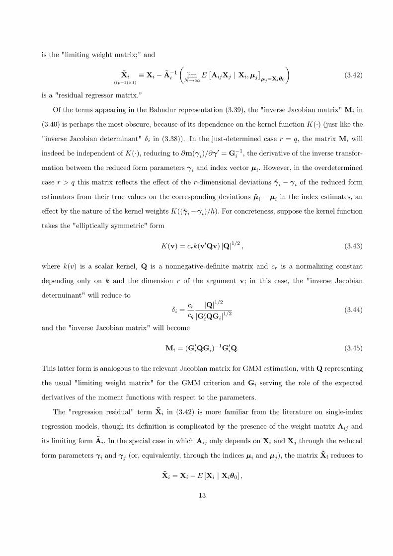
is the "limiting weight matrix;" and

Xi((p+1)×1)

≡ Xi − A−1i

(limN→∞

E[AijXj | Xi,µj

]µj=Xiθ0

)(3.42)

is a "residual regressor matrix."

Of the terms appearing in the Bahadur representation (3.39), the "inverse Jacobian matrix" Mi in

(3.40) is perhaps the most obscure, because of its dependence on the kernel function K(·) (jusr like the

"inverse Jacobian determinant" δi in (3.38)). In the just-determined case r = q, the matrix Mi will

insdeed be independent of K(·), reducing to ∂m(γi)/∂γ′ = G−1i , the derivative of the inverse transfor-

mation between the reduced form parameters γi and index vector µi. However, in the overdetermined

case r > q this matrix reflects the effect of the r-dimensional deviations γi − γι of the reduced form

estimators from their true values on the corresponding deviations µi − µi in the index estimates, an

effect by the nature of the kernel weights K((γi−γι)/h). For concreteness, suppose the kernel function

takes the "elliptically symmetric" form

K(v) = crk(v′Qv) |Q|1/2 , (3.43)

where k(v) is a scalar kernel, Q is a nonnegative-definite matrix and cr is a normalizing constant

depending only on k and the dimension r of the argument v; in this case, the "inverse Jacobian

deternuinant" will reduce to

δi =crcq

|Q|1/2

|G′iQGi|1/2(3.44)

and the "inverse Jacobian matrix" will become

Mi = (G′iQGi)

−1G′iQ. (3.45)

This latter form is analogous to the relevant Jacobian matrix for GMM estimation, with Q representing

the usual "limiting weight matrix" for the GMM criterion and Gi serving the role of the expected

derivatives of the moment functions with respect to the parameters.

The "regression residual" term Xi in (3.42) is more familiar from the literature on single-index

regression models, though its definition is complicated by the presence of the weight matrix Aij and

its limiting form Ai. In the special case in which Aij only depends on Xi and Xj through the reduced

form parameters γi and γj (or, equivalently, through the indices µi and µj), the matrix Xi reduces to

Xi = Xi − E [Xi | Xiθ0] ,

13

a familiar object in the large-sample theory for estimators of single-index or semiparametric regression

models.

The representation (3.39) facilitates the derivation of an asymptotic distribution theory for the

estimator θ = (1, β′)′ of the index coeffi cients. Under the assumptions imposed below, the terms

in this normalized average have zero mean and finite variance, so the Lindeberg-Levy central limit

theorem implies that Sθ0 is asymptotically normal. However, this asymptotic distribution will be

singular: since

θ′0X′i = θ′0X.i − A−1i lim

N→∞E[Aijθ

′0X′j | Xi,Xjθ0 = Xiθ0

](3.46)

= 0, (3.47)

it follows that√Nθ′0Sθ0 = op(1). (3.48)

This further implies that the smallest (in magnitude) eigenvalue ν converges in probability to zero

faster than the square root of the sample size, because

√N |ν| =

√N min

α 6=0|α′Sα|/‖α‖2 ≤

√N |θ′0Sθ0|/‖θ0‖

2 = op(1). (3.49)

To derive the asymptotic distribution of the proposed estimator β in (2.29), the normalized differ-

ence of β and β0 can be decomposed as

√N (β − β0) = [S22 − νI]−1

√n [S12 − (S22 − νI)θ0]

= [S22 − νI]−1√n s−

√n ν [S22 − νI]−1β0, (3.50)

where

s ≡ S12 − S22β0 ≡ [Sθ0]2, (3.51)

i.e., s is the subvector of Sθ0 corresponding to the free coeffi cients β0 . Using conditions (3.49), the

same arguments as in Ahn and Powell (1993) yield

S22 − ν I→p Σ22, (3.52)

where Σ22 is the lower p× p diagonal submatrix of Σ0, and also

√N (β − β0) = [Σ22]

−1√n s+ o(1), (3.53)

14

from which the consistency and asymptotic normality of θ follow from the asymptotic normality of

Sβ0. Specifically,√N (β − β0)→d N (0,Σ−122 Ω22Σ

−122 ), (3.54)

where Ω22 is the lower p× p diagonal submatrix of

Ω ≡ E[ψiψ′i], (3.55)

where ψi is the influence function term in (3.39), i.e.,

ψi ≡ 2φiX′iAiMiξi, (3.56)

A similar argument yields the asymptotic equivalence of the "closed form" estimator β of (2.30a) and

the estimator β, since

√N (β − β) =

√N([S22 − ν I]−1 − [S22]−1)S12

= −√N ν [S22 − ν I]−1θ (3.57)

= op(1),

for ν an intermediate value between ν and zero.

A final requirement for conducting the usual large-sample normal inference procedures is a consistent

estimator of the asymptotic covariance matrix Σ−122 Ω22Σ−122 of θ. Estimation of Σ−122 is straightforward;

by the results given above, either [S22 − νI]−1 or S−122 will be consistent, with the former being more

natural for θ and the latter for θ. Consistent estimation of the matrix Ω is less straightforward; given a

suitably-consistent estimator ψi of the influence function term ψi of (3.56), a corresponding estimator

of Ω could be constructed as

Ω ≡ 1n

n∑i=1

ψiψ′i. (3.58)

Estimation of ψi requires a corresponding estimator of the influence function term ξi for the estimator

of the reduced-form parameters, which would depend upon the form of these parameters—for example,

when γi = E [yi|Xi] , a natural estimator of ξi would be ξi = yi − γi = yi − E [yi|Xi] , Given an

appropriate estimator of the first-stage error term ξi,a similar Taylor’s series argument as in Ahn and

Powell (1993) yields a candidate ψi of an estimator of the second step influence function ψi,

ψi ≡2

n− 1

n∑i=1

1

hq+1D

(γi − γj

h

)ξi · (Xi −Xj)

′Aij(Xi −Xj), (3.59)

15

with D (v) ≡ ∂K(v)/∂v′. Verification of the consistency of Ω under the conditions imposed below

would follow the same strategy as described in Section 4 of.Ahn and Powell (1993).

4. The Ideal Weight Matrix

The results of the preceding section raise the question of the optimal choice of weight matrix

Aij to be used in the construction of S in (2.23) above. The usual effi ciency arguments suggest that

the optimal choice would yield equality (more precisely, proportionality) of the matrices Σ22 and Ω22

characterizing the asymptotic covariance matrix of θ. The matrices Σ0 and Ω0 can be expressed as

Σ0 = limN→∞

E[φi(Xi −Xj)Aij(Xi −Xj) |µi = µj ] (4.1)

= 2E[φiX

′iAiXi

](4.2)

and

Ω0 = 4E[φ2i X

′iAiMiViM

′iAiXi

], (4.3)

so the Gauss-Markov heuristic would suggest that the weight matrix A∗ij would be effi cient if the

corresponding limiting matrix A∗i equates 2Σ0 and Ω0, i.e., if

A∗i =(φiMiViM

′i

)−1, (4.4)

with corresponding matrices

2Σ∗0 = Ω∗0 = 4E[X′i(MiViM

′i

)−1Xi

]. (4.5)

Unfortunately, construction of a weight matrixA∗N (Xi,Xj) yielding A∗i of (4.4) through the relation

in (3.41) is apparently infeasible in the general setting in which Vi = Var [ξi|Xi] is a general function

of the regressor matrix Xi. However, in the special case that Vi is restricted to depend on Xi only

through γ(Xi) (or, equivalently, through the index vector Xiθ0), there is a matrix A∗ij yielding the

optimal limiting weight matrix A∗i of (4.4); that is, if

Vi ≡ Var [ξi|Xi]

= Var [ξi|Xiθ0] , (4.6)

16

then a sequence of matrices A∗N (Xi,Xj) for which

A∗ij ≡ limN→∞

A∗N (Xi,Xj) =

(φiMiViM

′i + φjMjVjM

′j

2

)−1(4.7)

would generate the limiting weight matrix in (4.4) and the corresponding equality of 2Σ∗0 and Ω∗0

in (4.5). The corresponding estimator β∗of the unnormalized slope coeffi cients β would have the

asymptotic normal distribution

√N (β

∗−β0) → dN (0,14[Ω∗22]

−1)

= N (0,(E[X′i(MiViM

′i

)−1Xi

]22

)−1), (4.8)

where now Xi = Xi − E [Xi | Xiθ0] due to the restricted form of A∗N (Xi,Xj). In the just-identified

setting with r = q, the matrices Mi and Vi are square, with Mi = G−1i , so the asymptotic distribution

of β∗would simplify to

√N (β

∗−β0)→d N (0,(E[X′iG

′iV−1i GiXi

]22

)−1). (4.9)

Even when condition (4.6) is imposed, the Gauss-Markov motivation for (4.4) would only establish

effi ciency of the estimator β∗within the class of estimators defined by (2.23), (2.29), and (2.30a), not

its effi ciency among all regular estimators of β0 under the restrictions imposed here. Still, for a special

case, a stronger semiparametric effi ciency result holds. The binary response model

yi = 1Xiθ0 + εi > 0

with independence of the error term εi and the (row vector of) regressors Xi will satisfy the index and

invertibility restrictions imposed here, with r = q = 1 and γi = E[yi|Xi] = g(Xiθ0), where g is the

c.d.f. of -εi (assumed invertible and smooth), Gi = dg(Xiθ0)/d(Xiθ0) = G′i, and Vi = γi(1− γi). For

this model, Klein and Spady (1993) propose an estimator of θ0 (up to scale) and shows that it achieves

the relevant semiparametric effi ciency bound, and with our normalization that effi cient estimator has

the same asymptotic distribution as β∗in (4.9), implying that β

∗is semiparametrically effi cient for

binary response under independence of the errors and regressors. For the just-determined multiple

index model (2.6), Lee (1995) shows that 4Ω∗22 is the semiparametric analogue of the information

matrix for estimation of β0 when only the index restrictions (2.6) (and smoothness of g(·) are imposed,

so β∗would have the same asymptotic distribution as an effi cient semiparametric estimator under these

17

index restrictions. However, the argument for consistency of β∗exploits the additional restriction of

invertibility of the conditional expections g(Xiθ0) in the vector of indicesXiθ0, which is not required for

consistency of Lee’s (1995) semiparametric maximum likelihood estimator. Indeed, Thompson (1993)

shows that, for the multinomial response model (2.4)-(2.5), the semiparametric information matrix

under the assumption of independence of the errors and regressors generally exceeds 4Ω∗22 when r > 1,

implying that the semiparametric effi ciency of β∗only holds for r = 1 (binary response).

As noted earlier, there is a close connection between the estimation approach proposed here and the

"minimum chi-squared logit" estimator proposed for the binary logit by Berkson (1955), and extended

to general parametric multinomial choice models by Amemiya (1976). For that estimation approach,

it is assumed that the matrix of regressors Xi is constant within each of a fixed number of groups, and

a nonparametric estimator of the vector of choice probabilities γi for each group is constructed from

the observed choice frequencies for each group. With this setup, the relavant asymptotic covariance

matrix Vi takes the form

Vi = diagγi − γγ ′, (4.10)

and information matrix

I = E[X′iG

′iV−1i GiXi

](4.11)

Amemiya (1976) shows that an effi cient estimator of θ0 for this setup is the coeffi cient vector of

the generalized least squares regression of g−1(γi) on Xi, using the matrix G′iV−1i Gi (or a feasible

version that replaces the unknown probabilities by the group frequencies) as the weighting matrix. The

estimator θ∗is a semiparametric analogue of this minimum chi-squared estimator, with asymptotic

variance similar to (4.11) but with the regressors Xi replaced by the residual regressors Xi = Xi −

E[Xi|Xiθ0].

When the index restrictiion (4.6) on the reduced-form error variance holds and the model is overde-

termined (r > q), there is another avenue to reduce the asymptotic variance of β, namely, choice of

kernel function K(·), which affects the asymptotic distribution of β through the inverse Jacobian ma-

trix term Mi. When this kernel function takes the elliptically-symmetric form (3.43) and the weight

matrix is the infeasible A∗ij of (4.4), the asymptotic variance of β∗is the inverse of the lower p × p

18

diagonal submatrix of

1

4Ω∗ = E

[X′i(MiViM

′i

)−1Xi

]= E

[X′i(G

′iQGi)

(G′iQViQGi

)−1(G′iQGi)Xi

], (4.12)

using the expression for Mi in (??). If Vi were constant (Vi ≡ V0), the usual Gauss-Markov heuris-

tic would choose Q to maximize this matrix by equating G′iQGi and G′iQVQGi, i.e., by setting

Q = Q∗ = V−1, so that the inverse of the asymptotic covariance matrix of β∗would reduce to

(1/4)Ω∗ = E[X′iG

′iV−10 GiXi

].When the covariance matrix Vi varies with Xi (but only as a function

of γi = g(Xiθ0)), this reduction would require a modification of the estimator S in (2.23), replacing

the the fixed kernel K(·) with a varying (elliptically symmetric) kernel K∗ij(·) of the form

K∗ij(v) = crk(v′Q∗ijv)

∣∣Q∗ij∣∣1/2 , (4.13)

with

Q∗ij ≡(

Vi +Vj

2

)−1. (4.14)

A modification of the arguments for the consistency and asymptotic normality of β would yield the

same results for the improved estimator β∗using the weight matrix A∗ij in (4.7) and the varying kernel

K∗ij(·) in (4.13), yielding the same form for the asymptotic distribution

√N (β

∗−β0)→d N (0,(E[X′iG

′iV−1i GiXi

]22

)−1). (4.15)

whether or not the model is just- or overdetermined.

Of course, even when condition (4.6) is imposed, the effi cient estimator θ∗using the ideal weight

matrix in (4.7) (and optimal kernel in (4.13)) would be infeasible in two respects —the limiting matrix

A∗ij does not specify the trimming mechanism needed to achieve the uniform nonparametric rate of

convergence of γi to γi specified in (??), and the construction of θ∗involves unknown nuisance para-

meters via the joint density function fµ(µi) of the indices, the Jacobian matrix Gi = ∂g(µi)/∂µ′, and

the reduced-form covariance matrix Vi. Following Ichimura (2004), the trimming requirement can be

imposed by multiplying the limiting A∗ij by a trimming term tij of trimming terms of the form

tij ≡ 1fX(Xi) > bN · 1fX(Xi) > bN, (4.16)

where fX(Xi) is the joint density function of the regressors and bN is a bandwidth term declining to zero

at an appropriate rate. Ichimura (2004) discusses conditions under which this trimming mechanism

19

will satisfy the requirements in (3.32) and also under which the asymptotic distribution S will be

unaffected by replacement of the density fX(Xi) in (4.16) by a consistent nonparametric (kernel)

estimator fX(Xi). As noted above, construction of a consistent estimator Vi of Vi will depend upon

the form of the reduced-form estimators γi; the remaining nuisance parameters fµ(µi) andGi could also

be consistently estimated using a kernel density estimator applied to the estimated indices µi = Xiθ

and the derivative of a kernel regression of γi on µi, respectively. Demonstration that an estimator

using a feasible version Aij of A∗ij would achieve the same asymptotic distribution (4.15) of the ideal

estimator β∗would involve strengthening of the regularity conditions and similar derivations to those

in the Appendix.

5. Appendix

The derivations of the consistency of S for Σ0 in (3.34) and the asymptotic linearity representation

(3.39) for Sθ0 follow the same lines as in Ahn and Powell (1993) and Blundell and Powell (2004).

Regarding S as a function of the reduced-form estimators γi and γj , a second-order Taylor’s series

expansion around the true reduced-form parameters γi and γj yields

S = S0 + S1 + S2, (5.1)

where

S0 ≡(N

2

)−1N−1∑i=1

N∑j=i+1

1

hqK

(γi − γj

h

)· (Xi −Xj)

′Aij(Xi −Xj), (5.2)

S1 ≡(N

2

)−1N−1∑i=1

N∑j=i+1

1

hq+1D

(γi − γj

h

)(γi − γi − γj + γj) · (Xi −Xj)

′Aij(Xi −Xj),

and

S2 ≡(N

2

)−1N−1∑i=1

N∑j=i+1

1

hq+2(γi−γi−γj+γj)′H

(γ∗i − γ∗j

h

)(γi−γi−γj+γj)·(Xi−Xj)

′Aij(Xi−Xj),

where D(v) ≡ ∂K(v)/∂v and H(v) ≡ ∂2K(v)/∂v∂v′, and where γ∗i and γ∗j are intermediate values.

The first term S0 is a second-order U-statistic with a summand depending on the sample size N

through the bandwidth term h. We assume that the terms in (Xi −Xj)′Aij(Xi −Xj) have bounded

second moments and have conditional expectations that are smooth functions of the underlying indices

20

Xiθ0 and Xjθ0, and also the kernel function K(·) satisfies some common regularity conditions (it

integrates to one, is bounded and continuous with bounded derivatives). Under such conditions, the

second moment of the terms in the summand for S0 will be of order h−q, so by Lemma 3.1 of Powell,

Stock, and Stoker (1989), the term S0 will satisfy a weak law of large numbers,

S0 − E [S0]p→ 0, (5.3)

provided

h = hN = o(1), h−q = o(N). (5.4)

Calculating the expectation of the summand in S0, first conditioning on µi = Xiθ0 and µj and then

making the change of variables u = (µi − µj)/h, yields

E [S0] = E

(h−qK

(g(µi)− g(µj)

h

)E[(Xi −Xj)

′Aij(Xi −Xj)∣∣µi,µj ])

= E

(∫K

(g(µi)− g(µi − hu)

h

)E[(Xi −Xj)

′Aij(Xi −Xj)∣∣µi,µj = µi − hu

]fµ(µi − hu)du)

→ E

(∫K (Giu) du·E

[(Xi −Xj)

′Aij(Xi −Xj)∣∣µi,µj = µi ] fµ(µi)) (5.5)

= E(δifµ(µi)(Xi −Xj)

′Aij(Xi −Xj)∣∣µi,µj = µi )

≡ Σ0.

Under the rate condition (3.32) for the uniform convergence of the reduced form estimators, the

remaining terms S1 and S2 in the decomposition (5.1) satisfy

‖S1‖ ≤2C

hq+1

( N

2

)−1N−1∑i=1

N∑j=i+1

∥∥(Xi −Xj)′Aij(Xi −Xj)

∥∥·[maxi,j

1||AN (Xi,Xj)|| 6= 0·||γ(Xi)− γ(Xi)||]

= op

(1

N3/8hq+1

), (5.6)

‖S2‖ ≤2C

hq+2

( N

2

)−1N−1∑i=1

N∑j=i+1

∥∥(Xi −Xj)′Aij(Xi −Xj)

∥∥·[maxi,j

1||AN (Xi,Xj)|| 6= 0·||γ(Xi)− γ(Xi)||2

]= op

(1

N3/4hq+2

)(5.7)

21

(where C is an upper bound for the kernel K and its first two derivatives). As long as the bandwidth

h converges to zero suffi cently slowly so that

1

h= o

(N1/4(q+2)

), (5.8)

it will follow that

‖S1‖ = op(1) (5.9)

and

‖S2‖ = op(N−1/2), (5.10)

implying

Sp→ Σ0. (5.11)

With the identification requirement that the lower p× p submatrix Σ22 has full rank, consistency of β

follows from Σ0θ0 = 0.

To obtain the asymptotic linearity condition (3.39), we use the same decomposition (5.1), yielding

√N Sθ0 =

√NS0θ0 +

√NS1θ0 +

√NS2θ0 (5.12)

=√

NS0θ0 +√NS1θ0 + op(1) (5.13)

by (5.10). The first term is a second-order smoothed U-statistic, so under condition (5.8), which implies

(5.4), Lemma 3.1 of Powell, Stock,and Stoker yield

√NS0θ0 =

√NE[S0θ0] +

2√N

N∑i=1

[ρiN − E [ρiN ]] + op(1), (5.14)

where

ρiN ≡ E

[h−qK

(g(µi)− g(µj)

h

)· (Xi −Xj)

′Aij(µi − µj) | Xj

]=

∫K

(g(µi)− g(µi − hu)

h

)E[((Xi −Xj)

′Aij (hu)∣∣Xi,µj = µi − hu

]fµ(µi − hu)du, (5.15)

again using the change-of-variables u =(µi−µj)/h for µj . Since the second moment of ρiN is of order

h2, it follows that√NS0θ0 =

√NE[S0θ0] + op(1), (5.16)

22

that is, that the only contribution of the leading term on the right-hand side of (5.12) is a bias term√NE[S0θ0]. Under the assumption that the expectation E[S0θ0] = E[S0θ0](h) is a suffi ciently smooth

function of the bandwidth parameter h, it will admit a power-series expansion of the form

E[S0θ0](h) =L∑j=1

Γjhj + o

(1√N

)(5.17)

as long as L is suffi ciently large so that hL+1 = o(N−1/2) while (5.8) is satisfied. Assuming the expansion

(5.17) is available, a kernel function K(·) can be constructed to ensure that the coeffi cient matrices Γj

equal zero for j = 1, ..., L using the jackknife approach described in Honoré and Powell (2004). (That

approach would replace the matrix S = S(h) by a particular linear combination of matrices S(cjh) for

distinct positive constants c1, ..., cL, which is algebraically equivalent to use of a "higher-order kernel"

constructed using the generalized jackknife approach of Schucany and Sommers (1977).) With this

choice of kernel, the bias term E[S0θ0] = o(N−1/2), which, together with (5.12) and (5.16), yields

√N Sθ0 =

√NS1θ0 + op(1). (5.18)

To verify the asymptotic linearity expression (3.39) for the remaining term√NS1θ0, we insert the

corresponding asymptotic linearity expression (2.21) into the expression for S1, obtaining

√NS1θ0 ≡

1√N

(N

2

)−1N−1∑i=1

N∑j=i+1

N∑l=1

1

hq+1D

(γi − γj

h

)(RlN (Xi)ξj −RlN (Xi)ξj)

·(Xi −Xj)′Aij(µi − µj)

+√N

(N

2

)−1N−1∑i=1

N∑j=i+1

1

hq+1D

(γi − γj

h

)(rlN − rlN )

·(Xi −Xj)′Aij(µi − µj)

≡ T1 +T2. (5.19)

The second term is asymptotically negligible under condition (3.33), since

‖T2‖ ≤C√N

hq+1

(N

2

)−1N−1∑i=1

N∑j=i+1

∥∥(Xi −Xj)′Aij(µi − µj)

∥∥ ·maxi,j

tij [||riN ||+ ||riN ||]

= Op

(N1/2h−(q+1)

)· op

(N−3/4

)= op

(N−1/4h−(q+1)

)= op(1), (5.20)

23

where the last line follows from condition (5.8) above (with C an upper bound for ‖D(·)‖).

Finally, apart from negligible terms with i = l or j = l, the term T1 can be rewritten as a third-order

smoothed U-statistic, i.e., it is of the form

T1 =√N

(N

3

)−1 ∑i<j<l

κijlN + op(1), (5.21)

where

κijlN ≡1

hq+1D

(γi − γj

h

)(RlN (Xi)ξj −RlN (Xi)ξj) · (Xi −Xj)

′Aij(µi − µj). (5.22)

Though the kernel κijlN is not symmetric in the indices i, j, and l, it can be symmetrized in the same

way as in the proof of Theorem 5.1 of Ahn and Powell (1993), by rewriting T1 as

T1 =√N

(N

3

)−1 ∑i<j<l

κijlN + op(1), (5.23)

where

κijlN ≡1

6(κijlN + κiljN + κjilN + κjliN + κlijN + κljiN ) . (5.24)

A crude bound for the second moment of κijlN is

E[‖κijl‖2] = O(E[‖RjN (Xi)‖2]

)·O(h−2(q+1)

)= O(N1/2h−2(q+1)),

under assumption (2.22), so this second moment will grow slower than the sample size N under (5.8),

which implies

h−2(q+1) = o(√N).

Thus the projection lemma for smoothed U-statistics (Lemma A.3 of Ahn and Powell 1993) implies

that the third-order U-statistic component of T1 can be replaced by its projection, i.e.,

T1 =6√N

N∑i=1

E[κijlN |ξi,Xi] + op(1).

Calculations analogous to those on pages 26 through 28 of Ahn and Powell (1993) establish that

E

[∥∥∥∥E[κijlN |ξi,Xi]−1

6ψi

∥∥∥∥] = o(N−1/2),

where ψi is the influence function term defined in (3.56), establishing the asymptotic linearity relation

(3.39).

24

6. References

Ahn, H., H. Ichimura, and J.L. Powell, 1996, "Simple Estimators for Monotone Index Models,"

manuscript, Department of Economics, University of California at Berkeley.

Ahn, H. and J.L. Powell, 1993, “Semiparametric estimation of censored selection models with a

nonparametric selection mechanism,”Journal of Econometrics, 58, 3-29.

Amemiya, T., 1976, "The maximum likelihood, the minimum chi-square, and the nonlinear weighted

least-squares estimator in the general qualitative response model," Journal of the American Statistical

Association, 71, 347-351.

Berkson, J., 1955, "Maximum likelihood and minimum χ2 estimates of the logistic function," Jour-

nal of the American Statistical Association, 50, 132-162.

Blundell, R.W. and J.L. Powell, 2004, "Endogeneity in Semiparametric Binary Response Models,"

Review of Economic Studies, 71, 655—679.

Han, A.K., 1987, “Non-parametric analysis of a generalized regression model: the maximum rank

correlation estimator,”Journal of Econometrics 35, 303-316.

Härdle, W. and T.M. Stoker, 1989, “Investigating smooth multiple regression by the method of

average derivatives,”Journal of the American Statistical Association, 84, 986-995.

Härdle, W. and J. Horowitz, 1996, “Direct Semiparametric Estimation of Single-Index Models With

Discrete Covariates,”Journal of the American Statistical Association, 91, 1632-1640.

Honoré, B.E. and J.L. Powell, 2005, "Pairwise Difference Estimators for Nonlinear Models," in

Andrews, D.W.K. and J.H. Stock, eds., ,Identification and Inference for Econometric Models, New

York: Cambridge University Press.

Ichimura, H., 1993, “Semiparametric least squares (SLS) and weighted SLS estimation of single-

index models,”Journal of Econometrics, 58, 71-120.

Ichimura, H,. 2004, "Computation of Asymptotic Distribution for Semiparametric GMM Estima-

tors," manuscript , Department of Economics, University Colleg London.

Ichimura, H. and L-F. Lee, 1991, “Semiparametric least squares estimation of multiple index models:

single equation estimation,”in: W.A. Barnett, J.L. Powell, and G. Tauchen, eds., Nonparametric and

semiparametric methods in econometrics and statistics, Cambridge: Cambridge University Press.

Klein, R.W. and R.S. Spady, 1993, “An effi cient semiparametric estimator of the binary response

25

model,”Econometrica, 61, 387-422.

Lee, L-F., 1995, "Semiparametric maximum likelihood estimation of polychotomous and sequential

choice models", Journal of Econometrics, 65, 385-428.

Manski, C.F., 1975, “Maximum score estimation of the stochastic utility model of choice,”Journal

of Econometrics, 3, 205-228.

Manski, C.F., 1985, “Semiparametric Analysis of discrete response, asymptotic properties of the

maximum score estimator,”Journal of Econometrics, 27, 205-228.

Newey, W.K. and P.A. Ruud, 2005, “Density weighted least squares estimation,” in Andrews,

D.W.K. and J.H. Stock, eds., Identification and Inference for Econometric Models, New York: Cam-

bridge University Press.

Newey, W.K. and T.M. Stoker, 1993 ”Effi ciency of weighted average derivative estimators and index

models,”Econometrica, 61, 1199-1223.

Powell, J.L., J.H. Stock and T.M. Stoker, 1989, “Semiparametric estimation of weighted average

derivatives,”Econometrica 57, 1403-1430.

Ruud, P.A., 1986, “Consistent estimation of limited dependent variable models despite misspecifi-

cation of distribution,”Journal of Econometrics, 32, 157-187.

Ruud, P.A., 2000, "Semiparametric estimation of discrete choice models," manuscript, Department

of Economics, University of California at Berkeley.

Schucany, W.R. and J.P.Sommers, 1977, "Improvement of kernel type density estimators, Journal

of the American Statistical Association, 72, 420-423.

Thompson, T.S. , 1993, "Some effi ciency bounds for semiparametric discrete choice models," Journal

of Econometrics, 58, 257—274

26