Simple Robust Linkages Between CDS and Equity Options

Peter Carra,b∗ Liuren Wuc†

aBloomberg L.P., 731 Lexington Avenue, New York, NY 10022, USA

bCourant Institute, New York University, 251 Mercer Street,New York, NY 10012, USA

cBaruch College, Zicklin School of Business, One Bernard Baruch Way, New York, NY 10010, USA

This version: January 15, 2008; First draft: September 25, 2007

Abstract

We test a theory that provides a simple and robust link between market prices of credit default swaps

(CDS) and equity options. The theory links the CDS spread to the market prices of vertical spreads of Amer-

ican put options which are sufficiently out-of-the-money. The linkage is established under a general class of

stock price dynamics for which the default event affects only the state space in which stock prices evolve.

Specifically, stock prices are assumed to be bounded below bya barrierB> 0 strictly before the default event,

and to drop below an alternative barrierA < B at the default time. We allow random stock price evolution

after default, so long as it is bounded above byA. We suppose that investors can take a static position in at

least two co-terminal American put options struck within the default corridor[A,B]. We show that a vertical

spread of such options scaled by the spread between the two strikes replicates a standardized credit insurance

contract that pays one dollar at default whenever the company defaults prior to the option expiry and zero

otherwise. Given the above state space behavior, we show that this simple replicating strategy is robust to the

details of the pre-default stock price dynamics, the post-default stock price dynamics, interest rate dynamics,

and default arrival rate fluctuations. We use the value of theAmerican put spread to infer risk-neutral default

probabilities and compare them to the default probabilities estimated from CDS spreads on the same reference

company. Collecting data from both markets on several reference companies with significant default proba-

bilities, we identify a strong correlation between the default probabilities inferred from the two markets, and

find that deviations between the two estimates help predict future movements in both markets.

JEL Classification:C13; C51; G12; G13.

We are grateful to Bruno Dupire, Bjorn Flesaker, Ziqiang Liu, Dilip Madan, Eric Rosenfeld, Ian Schaad, Serge Tchikanda,ArunVerma, and Yan Wang for discussions and comments. We welcomecomments, including references that we have inadvertentlymissed.

∗Tel.: +1-212-617-5056; fax: +1-917-369-5629.E-mail address:pcarr4@bloomberg.com.†Tel.: +1-646-312-3509; fax: +1-646-312-3451.E-mail address:liuren wu@baruch.cuny.edu.

Keywords:Stock options; American puts; credit default swaps; default arrival rate; default probabilities.

2

Contents

1 Introduction 1

2 Theory 4

2.1 A tale of two generalizations . . . . . . . . . . . . . . . . . . . . . . .. . . . . . . . . . . . 5

2.2 Defaultable displaced diffusion: A toy example . . . . . . .. . . . . . . . . . . . . . . . . . 7

2.2.1 Transition probability density function . . . . . . . . . .. . . . . . . . . . . . . . . . 9

2.2.2 Pricing American put options . . . . . . . . . . . . . . . . . . . . .. . . . . . . . . 10

2.2.3 Linking American put spreads to unit recovery claims .. . . . . . . . . . . . . . . . 11

2.3 Defaultable displaced diffusion: The general specification . . . . . . . . . . . . . . . . . . . . 12

2.4 Linking unit recovery claims to CDS spreads . . . . . . . . . . .. . . . . . . . . . . . . . . 16

3 Data and estimation 17

3.1 Inferring default probabilities from American put spreads . . . . . . . . . . . . . . . . . . . .18

3.2 Inferring default probabilities from CDS spreads . . . . .. . . . . . . . . . . . . . . . . . . 19

3.3 Replicating unit recovery claims from both markets . . . .. . . . . . . . . . . . . . . . . . . 20

4 Results 20

4.1 Predicting the movements of unit recovery claims . . . . . .. . . . . . . . . . . . . . . . . . 24

5 Alternative linkages 25

6 Concluding remarks 28

A Conditional transitional probability density function under the toy DDD model 30

3

1. Introduction

Notional amounts in both credit and equity derivatives continue to display strong growth. In September

2007, the International Swaps and Derivatives Association, Inc. (ISDA) announced that the notional amounts

outstanding of credit derivatives grew by 75% to $45.46 trillion from $26.0 trillion one year earlier, and the

notional amounts in equity derivatives grew by 57% to $10.01trillion from $6.38 trillion one year earlier. As

a result of the continued strong growth in both markets, there is strong interest in understanding if and how the

two markets are linked. If the payoffs are linked but the prices are not, trading opportunities arise. If payoffs

and prices are both linked, the understanding of each marketcan be substantially improved by integrating the

two markets.

For the ISDA survey, credit derivatives comprise credit default swaps referencing single names, indexes,

baskets, and portfolios; equity derivatives comprise equity swaps, options, and forwards. In this paper, we

focus on two segments of the credit and equity derivatives markets that show particularly strong linkages. On

the credit derivatives side, we focus on credit default swaps (CDS) written on a corporate bond, which remains

the largest segment by volume. On the equity derivatives side, we focus on American options written on the

stock of the corresponding firm that issued the corporate bond. While there is much literature attempting to

link single name CDS with single name stock options, the focus to date has been on European-style options.3

This focus is unfortunate since for single name stock options, the only transparency in pricing arises from

listed options, which are all American style. We conjecturethat the past focus on linkages between CDS and

European options stems from the greater ease with which prices of European options can be analytically re-

lated to the underlying stock prices in standard option pricing models. In contrast, the problem of analytically

relating American option prices to the underlying stock price is notoriously difficult.

In this paper, we show that the spread between two American put options with a particular strike range can

be used to directly synthesize a standardized credit insurance contract that pays one dollar at default whenever

the company defaults prior to the option expiry and zero otherwise. This direct linkage between American

put options and credit contracts holds true under a wide class of stock price dynamics. The key assumption

for this class of price dynamics is that random stock prices are bounded below by a barrierB > 0 before

default and drop below an alternative barrierA∈ [0,B) at default. After the default time and before expiry, the

stock price dynamics are bounded above byA. As long as these conditions are satisfied, the simple linkage

3Examples include Bakshi, Madan, and Zhang (2006), Carr and Wu (2005), Collin-Dufresne, Goldstein, and Martin (2001),Cremers, Driessen, Maenhout, and Weinbaum (2004), and Hull, Nelken, and White (2004).

1

holds robustly, irrespective of the details of the stock price dynamics before and after default, the interest rate

dynamics, and default arrival rate fluctuations.

Classic structural models of default, e.g., Merton (1974),have the property that prior to default, the firm

value is random and bounded below by the default barrier. In such models, stock prices vanish at default

and remain zero afterwards. In a recent paper, Carey and Gordy (2007) show that private debtholders play

a key role in setting the endogenous asset value threshold below which corporations declare bankruptcy. In

particular, the private debtholders often find it optimal toforce the bankruptcy well before equity values

vanish. Our specification of the stock price dynamics is in line with such evidence.

Suppose that investors can take static positions in at leasttwo American put options of the same maturityT

and whose strikes(K1 > K2) lie within the default corridor(A,B). Given that the stock price is bounded below

by B > 0 before default, and is bounded above byA < B at and after default, then a simple vertical spread

of the two American put options scaled by the strike distance, Ut(T) ≡ (Pt(K1,T)−Pt(K2,T))/(K1 −K2),

replicates a standardized credit insurance contract that pays off one dollar whenever default occurs up to the

option expiry and zero otherwise. Without default, the stock price stays aboveK1, and hence both put options

will not be exercised as they always have zero intrinsic value. If default occurs prior to the option expiry, then

the stock price falls belowK2 and stays below it afterwards. We will show that both optionsare optimally

exercised at the default time as a result, so that the scaled spread nets a payoff of one dollar at this time. If we

further assume that the stock price falls to zero at the default time (A = 0), then we can setK2 = 0 and use a

single American put option to construct this credit insurance contract,Ut(T) = Pt(K1,T)/K1.

We refer to this standardized credit contract as aunit recovery claim.4 This fundamental claim is simply

a fixed-life Arrow Debreu security paying off one dollar whenthe (default) event occurs, and zero otherwise.

Since American put options trade simultaneously at severaldiscrete maturities, it is possible to interpolate

and extrapolate in the maturity dimension to obtain a term structure of synthetic unit recovery claims. By

assuming deterministic interest rates, we can readily compute the risk-neutral default probabilities from this

term structure.

To link the American stock options to the credit default swap(CDS) spreads on the same reference com-

pany, we assume that the recovery rate on the corporate bond underlying the CDS contract is known. Then,

the value of the protection leg of the CDS contract becomes proportional to the value of the unit recovery

claim, which we can replicate using two American put options. Once the value of the protection leg becomes

4The Chicago Board of Options Exchange (CBOE) has recently launched unit recovery claims under the name Credit EventBinary Option (CEBO).

2

a known function of its maturity, one can uniquely determinethe CDS spread curve by further assuming de-

terministic interest rates. Alternatively, one can take the CDS spread curve as given, strip it for the value of

the protection leg, and then back out the implied recovery rate on the bond using the observable American put

spread.

To empirically test the strength of the linkage between the two markets, we choose eight reference com-

panies from the components of the North American High Yield CDS Index (CDX). The Index is composed of

100 non-investment grade entities, distributed amoung three sub-indices: B, BB, and HB. The composition of

the high yield index and each sub-index is determined by a consortium of 16 member banks. The indices roll

every six months in March and September of each year. We take the 100 components from the index rolled

out in September of 2007 and take eight companies that we haveviable quotes on both CDS and American

put options. The CDS quotes are obtained from Bloomberg. TheAmerican options quotes are obtained from

OptionMetrics. We take the sample period from January 2005 to June 2007. From the options data set, at each

date we synthesize the value of the unit recovery claim at allobservable maturities, compute the risk-neutral

default probabilities while assuming deterministic interest rates, and interpolate to obtain the risk-neutral de-

fault probability at one-year fixed time-to-maturity. Fromthe CDS data, we use the one-year CDS spread to

also compute the one-year risk-neutral default probabilities assuming fixed bond recovery rates and determin-

istic interest rates. Then, we compare the two time series ofdefault probabilities for each reference company.

First, we find that the strike choices in defining the Americanput spread can induce some biases in the default

probability estimates. Nevertheless, the probabilities obtained from the American put spreads are on average

close to those computed from the CDS spread. Furthermore, for each company, the two time series of default

probabilities show high cross-correlations, especially when the default probability is significant. The cross-

correlation estimates are over 80% when the default probabilities are over 2%. Furthermore, we find that

deviations between the two default probability estimates can help predict future movements in both markets.

In linking credit insurance to American equity options, we make assumptions on the stock price dynamics

that lie between structural and reduced-form models. As in structural models, we assume that default occurs

the first time that the stock price crosses a lower barrier, which does not need to be constant but nevertheless

needs to have a fixed lower bound. As in reduced form models, weassume that the waiting time to default

is completely unanticipated. The main innovation in our specification is that the default barrier is expanded

into adefault corridor(A,B). The stock price is assumed to evolve randomly above the default corridor prior

to the default time, to drop below the default corridor at default, and to evolve deterministically afterwards.

It is these three behavioral modes that generate the tight linkage between the American options and the CDS

3

markets.

For comparison, we also implement a simple version of Merton(1974)’s structural model to compute the

one-year default probabilities by using information in thecapital structure and the return volatility. In the

implementation, we use stock price to proxy the per share equity value, net debt per share to proxy the per

share face value of debt, and one stock option implied volatility to proxy for return volatility. Based on these

inputs, we compute the firm value and firm volatility, with which we compute the risk-neutral probability that

the stock price will stay above the face value of the debt at the one-year horizon. We use one minus this

probability as a measure for the one-year risk-neutral default probability from this model. We find that the

default probabilities estimated from the structural modelare significantly lower than those obtained from the

American puts or those from the CDS spreads. Nevertheless, the estimates can show high cross-correlations

with the default probabilities inferred from the CDS spread, especially if we use the implied volatility of

out-of-the-money American put options as the stock return volatility input. This exercise shows that the real

information in the stock market on credit risk is in out-of-the-money put options, as we have shown in our

simple robust linkage.

The rest of the paper is structured as follows. The next section lays down the theoretical framework,

under which we build the tight linkage between the American stock options market and the CDS market.

In this section, we first review two simple generalizations of the standard option pricing model proposed by

Black and Scholes (1973) and by Merton (1973). Then we combine the two generalizations to set up a toy

example of our modeling framework under which we can price American options analytically and link the

American put spreads to unit recovery claims. Finally, we specify the general class of models, under which

the simple linkage between American put spreads and CDS spreads remain robust. Section 3 describes the

data that we use for our empirical work and the procedure thatwe follow to estimate one-year risk-neutral

default probabilities from the two markets. Section 4 compares the two time series of default probabilities

for each company. Section 5 estimates the risk-neutral default probability from a simple structural model

and compares the estimates to those obtained from the American puts and the CDS market. Section 6 offers

concluding remarks and directions for future research.

2. Theory

Black and Scholes (1973) and Merton (1973) propose an optionpricing model, henceforth the BMS

4

model, that has since revolutionized the derivative industry. The main assumptions underlying the BMS

model are that investors can trade continuously over time, that sample paths of the underlying stock price

are continuous, and that the stock’s return volatility is constant. As the model also assumes no arbitrage and

constant proportional carrying costs for the stock, the risk-neutral stock price process is simply geometric

Brownian motion. When this diffusion process is started from a positive level, it can never hit zero.

In what follows, we first review two generalizations of the BMS model proposed by Merton (1976) and

Rubinstein (1983), respectively. Inspired by these generalization, we propose our modeling framework, under

which we build the linkages between credit insurance and American equity options.

2.1. A tale of two generalizations

For companies with positive default probabilities, the stock price going to zero is a definite possibility.

After a company defaults, its stock price is likely to be low and it is common to assume that the stock price

is in fact zero after bankruptcy. Recognizing that the underlying stock price dynamics in the BMS model

are not consistent with this default-related behavior, Merton (1976) generalizes the dynamics by allowing the

possibility for the stock price to jump to zero. We refer to this model as the Merton-Jump-to-Default model

or simply MJD. As the stock of a company is a limited liabilityasset, the MJD model realistically assumes

that the stock price remains at zero after the jump time.

Assuming that the risk-neutral arrival rate of such a jump isconstant, we can still replicate the payoff of

a European call option in the MJD model by dynamically trading just the stock and a corporate bond whose

value also vanishes upon default. The addition of the bankruptcy state does not destroy our ability to replicate

the payoff of the call option as long as we can use a corporate bond instead of a default-free bond as a hedge

instrument. The reason is that the value of the target call option and the value of the stock-bond hedging

portfolio both vanish upon default.

Since the payoff of the call option can be replicated, its price is uniquely determined by no arbitrage.

Merton (1976) shows that the only effect on the BMS call pricing formula of using the MJD model is to cause

the stock growth rate and call discount rate to both increaseby the risk-neutral default arrival rate. The reason

for these changes becomes clear once we recognize that the option pricing formula relates the call price at

any future time to the contemporaneous stock price, conditioning on no prior default. The requirement that

the unconditional risk-neutral expected return on the stock and the call both be the riskfree rate forces the

conditional growth rate in each asset to be higher, as the values for both assets drop to zero upon default.

5

Since each asset drops by 100% of its value, the conditional growth rate of each asset must exceed the riskless

rate by the default arrival rate.

Once the linkage between the value of a European call and its underlying stock has been established, the

link between the value of a European put and its underlying stock is established by put-call parity. Merton

(1976) does not address the pricing of American options, butit is straightforward to analyze the impact of a

jump to default on the optimal exercise strategy. When the underlying stock pays sufficiently small dividends,

it is still the case that American calls are not exercised early (see Merton (1973)). So long as the riskfree

rate is positive and dividends are sufficiently small, it is also still the case that American puts always have

positive probability of early exercise. As in the case with no jump to default, the optimal exercise strategy is

to exercise the American put once the stock price enters a stopping region. As this region contains the origin,

the American put will be exercised early if there is a jump to default. It will also be exercised early if the

stock price diffuses down to an exercise boundary. The analytic determination of this exercise boundary is a

difficult problem and is the main hindrance in analytically valuing American puts in either the MJD or BMS

model.

The MJD model extends the BMS model to include bankruptcy while preserving tractability. In evaluating

the validity of any extension of the BMS option pricing model, it is common to use the notion of option implied

volatility. The implied volatility of an option is defined asthe constant volatility input that one must supply

to the BMS option pricing model in order to have the BMS model value agree with a given option price.

The given option price can be produced by either the model or the market and hence implied volatilities can

likewise be produced by either the model or the market. The model implied volatility of the BMS model is

invariant to strike price. In contrast, the model implied volatility of the MJD model is always decreasing in

the strike price, generating what is commonly referred to asan implied volatility skew.

Motivated by the possibility of producing an analytically tractable European option pricing model for

which implied volatilities can decrease or increase in strike, Rubinstein (1983) introduces the displaced dif-

fusion option pricing model, henceforth the RDD model. In this model, Rubinstein relaxes the requirement

in the BMS model that the state space of the underlying stock price diffusion be the whole positive real line.

Specially, letS0 > 0 denote the initial stock price, Rubinstein introduces a new parameterB∈ (−∞,S0). As-

suming a constant interest rater, an initial investment ofB in the riskfree asset would grow toBert by time

t. Rubinstein suggests that the risk-neutral process for theunderlying stock price be constructed by summing

Bert with a geometric Brownian motion. As a result, the state space of the underlying stock price process at

6

any timet is (Bert ,∞) rather than(0,∞).

As with the MJD model, Rubinstein’s displaced diffusion is an extension of the BMS model while main-

taining the analytical tractability. However, the RDD model has some properties that are not shared by either

the BMS or MJD model. In particular, ifB is positive, levels in(0,Bert ) cannot be reached by the stock price.

It can be shown that the implied volatilities produced by this positively displaced diffusion are an increas-

ing function of strikeK ∈ (Bert ,∞). If B is negative, levels in(Bert ,0) can be reached by the stock price,

and the implied volatilities produced by the negatively displaced diffusion are a decreasing function of strike

K ∈ (Bert ,∞). The RDD model collapses to the standard BMS model when the displacementB is zero.

It is interesting to compare the two generalizations of the BMS, the MJD and the RDD model. Merton’s

generalization introduces a scale factoreλt on the allowed sample paths, while Rubinstein’s generalization

introduces a shiftBert . Under MJD model, the underlying stock price has a state space of [0,∞) and the model

implied volatility can only stay constant or decline in strike price. Under RDD, the underlying stock price has

a state space at timet of (Bert ,∞) and the model implied volatility either increases with the strike whenB> 0

or decreases with the strike whenB < 0. Neither model can produce a U-shaped relation between implied

volatility and strike price, a shape that is the most commonly observed in the market and is often referred

to as the implied volatility smile. To generate smile-consistent dynamics, we propose to combine the two

generalizations to both scale and shift the sample paths.

2.2. Defaultable displaced diffusion: A toy example

Before we lay out the general model specification, we start with a toy example to illustrate the ideas behind

the linkage between credit spreads and the value spread of two American puts. Our specification allows for

both default as in the MJD model and diffusion displacement as in the RDD model. Taken together, we label

the class of models that we propose asdefaultable displaced diffusion, or the DDD model.

As in earlier generation models, we assume frictionless markets, no arbitrage, and the existence of a

riskfree asset with strictly positive paths of bounded variation. As a result, there exists a risk-neutral measure

Q under which all tradeable securities have an expected return equal to the riskfree rate. We useT to denote

the common expiry date of the options and credit contracts. We assume that the underlying stock pays no

dividends over[0,T] and we letr ≥ 0 be the assumed constant riskfree rate over this horizon.

To intuitively describe the risk-neutral stock price dynamics in the toy DDD model, we start with the stock

7

priceSfollowing Rubinstein (1983) displaced diffusion over the fixed time horizont ∈ [0,T]. The stock price

process is assumed to be positively displaced, withB∈ (0,S0]. Then, we depart from Rubinstein’s model by

adding the possibility of a down jump in the stock price. If the first jump in the stock price happens to occur

at timeT, we assume that the stock price jumps to some constantR∈ [0,B). More generally, if the stock price

jumps at some timet ∈ [0,T], we assume that it jumps to the deterministic recovery levelR(t) ≡ Re−r(T−t).

After the jump timeτ, the stock price grows deterministically at the riskfree rate r, i.e. St = R(t) for t ≥ τ.

The risk-neutral arrival rate of the jump in the stock price is assumed to be constant atλ ≥ 0.

To formally model the risk-neutral stock price dynamics in the toy DDD model, we introduce a standard

Brownian motionW and a standard Poisson processN with intensityλ. We letG be a geometric Brownian

motion defined by

Gt = eσWt−σ2t/2, (1)

with G0 = 1 and whereσ is a real constant. The random processG is a martingale started at one. We letJ be

another martingale started at one defined by

Jt = 1(Nt = 0)eλt . (2)

This process drifts up at a constant growth rate ofλ and jumps to zero and stays there at a random and

exponentially distributed time. It is easy to see thatG andJ are both martingales since equations (1) and (2)

imply that they respectively solve the following stochastic differential equations,

dGt = σGtdWt , dJt = −Jt−(dNt −λdt), (3)

where the subscriptt− indicates that the pre-jump level is used at timet. As a result,J is a right continuous

left limits (RCLL) process.

We construct the stock price processSby combining the two random processesG andJ as

St− = ert{R(0)+Jt−[B−R(0)+ (S0−B)Gt]}. (4)

To understand this RCLL stock price process, we can rewrite the stock price process as the sum of three

components,

St− = R(0)ert +[B−R(0)]ert Jt− +(S0−B)ert Jt−Gt . (5)

8

Each component has the form of a constant, multiplied byert , and then a martingale. Therefore, each com-

ponent can be interpreted as the time-t value resulting from investing the constant in an asset whose initial

price is one. In this sense, we are attributing the equity value of a firm to returns from three types of in-

vestments. The first type is a riskless cash reserve defined bythe deterministic and non-negative process

R(t) = R(0)ert . The second type is a defaultable risky cash reserve defined by the stochastic and non-negative

process[B−R(0)]ert Jt−, with the martingaleJt− capturing the default risk. The third type of investment is a

defaultable and market risky asset defined by the stochasticand non-negative process(S0−B)ert Jt−Gt , with

the martingaleGt capturing the market, diffusion-type variation.5 Under the risk-neutral measureQ, all three

investments generate a risk-neutral expected return ofr.

From equation (4), we can derive the stochastic differential equation for the stock price dynamics,

dSt = rSt−dt− (St−−R(t))(dNt −λdt)+{St−− [R(t)+ (B−R(0))Jt−ert ]}σdWt , (6)

where the exposures to the martingale incrementsdNt − λdt anddWt are both affine in the stock priceSt−.

Since no jumps occur before default, the pre-default stock price dynamics simplify to,

dSt = [rSt− + λ(St−−R(t))]dt+{St−− [R(t)+eλt [Bert −R(t)]}σdWt , t ∈ [0,τ), (7)

where both drift and the diffusion coefficient of the stock price dynamics are affine in the stock price.

If we set λ = 0 in the toy DDD model, the model degenerates to the positively displaced diffusion of

Rubinstein (1983), for which implied volatility increaseswith strike. Conversely, if we setB = 0, the model

degenerates to Merton (1976)’s MJD model, for which impliedvolatility decreases with strike. Whenλ and

B are both positive, the implied volatility smiles when graphed against the strike price. This model behavior

is broadly consistent with the behavior of implied volatilities obtained from market prices of listed American

stock options.

2.2.1. Transition probability density function

In this toy model, the transition probability density function (TPDF) of the stock price can be derived in

closed form. LetK(t) ≡ R(0)ert +[B−R(0)]e(r+λ)t. For K > K(T) andS> K(t), the TPDF conditional on

5The stock price dynamics can also have jumps. For simplicity, we exclude this possibility in our toy example, but we incorporatejumps in the general DDD specification.

9

surviving toT is6

Q{ST ∈ dK|St = S,NT = 0} =exp{−[lnh(K,S)+ σ2(T − t)/2]/σ

√T − t]2/2}

√

2πσ2(T − t)

1

K−R− [B−R(0)]e(r+λ)T.

(8)

The risk-neutral probability of defaulting over[t,T] is simply 1− e−λ(T−t) and this is also the risk-neutral

probability thatST = R, given thatSt = S> K(t). One can easily use these results to develop closed form

formulas for European options. As no listed single name stock options are European, we leave this as an

exercise to the interested reader.

2.2.2. Pricing American put options

Prior to default,Jt = eλt andGt > 0, so (5) implies that the stock priceSt exceedsB(t) ≡ R(0)ert +[B−R(0)]e(r+λ)t . At the default timeτ, Jτ = 0, and the stock price jumps down to the riskless cash reservelevel

R(τ)≡ Re−r(T−τ). After the default, the stock priceSt = Re−r(T−t). SinceK(t) ≥ B andR(t)≤ R, we observe

that the stock price process is random and at leastB in the pre-default periodt ∈ [0,τ ∧T], and becomes

deterministic and at mostR in the post-default period,t ∈ [τ,T]. These special properties allow us to derive a

closed-form solution for the value of of American puts struck belowB.

Let K denote the strike price of an American put maturing atT. If K ∈ [0,R(0)], the put is worthless since

it cannot finish in the money in the toy DDD model. IfK ∈ (R(0),R], at any timet before default, the stock

price is aboveB and hence the strike priceK. To define the continuation and exercise regions, lett∗ solve

Re−r(T−t∗) = K. If default occurs at some timeτ in (0, t∗), thenSτ < K and it is optimal to exercise atτ. If

default occurs in[t∗,T], thenSτ ≥ K and it is better to hold on to the American put and let it expireworthless.

Therefore, for such puts, the continuation region is the union of all stock prices aboveB(t) and the curve

R(t), t ∈ [t∗,T], while the exercise region is just the curveR(t), t ∈ [0, t∗]. The payoff from holding such an

American put isK −R(τ) at timeτ if τ ≤ t∗ and zero otherwise. LetP0(K,T) denote the time-0 value of an

American put. By risk-neutral valuation, we have,

P0(K,T) = EQ{e−rτ[K−R(τ)]1(τ ≤ t∗)} =

Z t∗

0λe−λte−rt [K−Re−r(T−t)]dt

= λ

[

K1−e−(r+λ)t∗

r + λ−Re−rT 1−e−λt∗

λ

]

. (9)

6Refer to Appendix A for a proof.

10

If K ∈ (R,B], thent∗ > T and hence the continuation region is all stock prices aboveB(t), while the exercise

region is just the curveR(t), t ∈ [0,T]. The put value is obtained by simply replacingt∗ with T in equation (9),

P0(K,T) = λ

[

K1−e−(r+λ)T

r + λ−Re−rT 1−e−λT

λ

]

. (10)

For American puts options struck aboveB, finite difference methods can be used to numerically approx-

imate the American put valueP(S, t) and the free boundaryS∗(t), t ∈ [0,T]. For S> S∗(t), t ∈ [0,T], the

American put valueP(S, t) solves the partial differential equation,

[

G +∂∂t

]

P(S, t) = rP(S, t), (11)

where

G ≡ σ2

2{S− [R(t)+eλt [Bert −R(t)]}2 ∂2

∂S2 +{rS+ λ[S−R(t)]} ∂∂S

, (12)

subject to the terminal condition

P(S,T) = (K−S)+, S> S∗(T), (13)

and the boundary conditions:

limS↓S∗(t)

P(S, t) = K−S∗(t) and limS↓S∗(t)

∂∂S

P(S, t) = −1, t ∈ [0,T]. (14)

For S≤ S∗(t), t ∈ [0,T], the American put valueP(S, t) = K−S.

2.2.3. Linking American put spreads to unit recovery claims

Now suppose that we observe the market prices of at least two out-of-the-money American put options of

maturity T. Let K1 andK2 denote the associated strike prices and we require thatR≤ K1 < K2 ≤ B. Since

St ≥ B prior to the default time, we know that neither put will be exercised if the firm survives toT. In

contrast, if the firm defaults at some timeτ beforeT, sinceSτ ≤ K1 and grows deterministically thereafter,

both puts will be exercised atτ. Let △K ≡ K2−K1 and△P0(T) ≡ P0(K2,T)−P0(K1,T), whereP0(K1,T)

andP0(K2,T) are the two observable put option prices. Suppose that an investor buys 1△K units of theK2 put

and writes an equal number of theK1 put, the cost of this position is△P0(T)△K , which we refer to as the American

11

put spread.

If no default occurs prior to expiry (τ > T), the American put spread expires worthless. Ifτ ≤ T, the

American put spread pays out one dollar so long as both parties behave optimally. Furthermore, so long as

the American put prices are consistent with optimal behavior as is usually assumed, these prices can be used

to value credit derivatives.

To illustrate this point, consider aunit recovery claim, which pays one dollar atτ if τ ≤ T and zero

otherwise. LetU0(T) denote the arbitrage-free spot value of this claim. In the toy DDD model, this value is

U0(T) =

Z T

0λe−(r+λ)tdt = λ

1−e−(r+λ)T

r + λ. (15)

Unfortunately, if the only assets with observable prices are the riskfree asset and the stock, one cannot infer the

required inputλ. Fortunately, if the observable prices are those of two American putsP0(K2,T) andP0(K1,T),

hten no arbitrage dictates that the value of this unit recovery claim is equal to the value of the American put

spread:

U0(T) =△P0(T)

△K. (16)

As we will show, this simple equation holds under much more general conditions and can be regarded as the

fundamental result of this paper.

Furthermore, under the toy DDD model, we can equate the two right hand sides of equations (15) and (16)

to numerically determineλ from the observation of the riskfree rater and the American put spread△P0(T)△K . As

a result, we can compute the risk-neutral default probability over a fixed horizon[0,T] as 1−e−λT .

2.3. Defaultable displaced diffusion: The general specification

The toy DDD model places strong restrictions on the stock price dynamics to show clearly the tight

linkages between American put spreads and default contingent claims. In this subsection, we show that the

fundamental linkage as shown in equation (16) remains valid, even if we relax the assumptions of the toy

DDD model substantially. In particular, we can generalize the toy model along four major dimensions.

• Random Interest Rates: In the toy DDD model, the riskfree interest rate is fixed as a constant. In

the general specification, we allow the spot interest rater to be a nonnegative stochastic process. As

a result, there exists a money market account whose initial balance is one and whose balance at time

12

t ∈ [0,T] is given byβt ≡ eR t

0 rsds. No arbitrage dictates that there exists a probability measureQ under

which the gains process from any admissible trading strategy deflated byβ is a martingale.

• Random Stock Recovery: In the toy DDD model, the stock price evolves randomly aboveB prior

to default, while the recovery valueR(t) evolves deterministically below a levelR< B afterwards. In

the general DDD class of stochastic processes, the stock price can be random at the default time and

afterwards, but it must evolve below a barrierA < B in any post-default periodt ∈ [τ,T]. To define

these post-default dynamics, let(A,B) be the default corridor withA≥ 0 andB< S0. Let Rt be the spot

price of an asset with support[0,A] over [0,T]. We may write its stochastic differential equation as:

dRt = rtRtdt+dMRt , t ∈ [0,T], (17)

whereMR is aQ martingale. We simply setSt = Rt in any post-default periodt ∈ [τ,T].

• Stochastic Default Arrival: In the toy DDD model, the risk-neutral default arrival rate is constant. In

the generalization, the risk-neutral default arrival rateλ is a nonnegative stochastic process. We define

Jt = 1(Nt = 0)eR t

0 λsds whereN is now a counting process. We note thatJ is a stochastic exponential

since it solves:

dJt = −Jt−[dNt −λtdt]. (18)

Furthermore sinceNt −R t

0 λsdsis a martingale, so isJ. We require that the martingaleJ be independent

of the processR.

• Stochastic Volatility and Jumps: In the toy DDD model, the market risk driver is a Geometric Brow-

nian Motion, denoted asGt . In the general specification, we allow the market risk driver G to be the

stochastic exponential of a martingaleMG, i.e., Gt = E (MG). As a result,G still starts at one and is

still a martingale since

dGt = Gt−dMGt . (19)

The processG is now allowed to jump, but we assume that jumps inMG are bounded below by -1, so

thatG is nonnegative. We furthermore require that the martingaleG be independent of the martingale

J. In contrast,G can depend onr, λ, andR.

To contend with this four dimensional generalization, we construct the stock price process as:

St = (1−Jt)Rt +eR t

0 rsdsJt [B+(S0−B)Gt] , (20)

13

whereR0− ≡ R0. We can again expressSas the sum of three stochastic processes,

St = Rt −JtRt +eR t

0 rsdsJt [B+(S0−B)Gt ], t ∈ [0,T). (21)

For t ∈ [0,τ∧T], the first termRt is clearly an asset price process, as indicated in equation (17). Since the

martingaleJ is a stochastic exponential and is orthogonal toR, the productJRis also an asset price process for

t ∈ [0,τ∧T]. Since the martingalesJ andG are orthogonal, the processJt [B+(S0−B)Gt] is also a martingale.

As a consequence, the last term in (21) is an asset price process. It follows thatS is also an asset price process

for t ∈ [0,τ∧T]. SinceNt = 0 andJt = eR t

0 λsds prior to default, the stock price dynamics overt ∈ [0,τ∧T) can

also be written as,

St = Rt [1−eR t

0 λsds]+eR t

0(rs+λs)ds[B+(S0−B)Gt]. (22)

The stochastic differential equation that governs the stock price process prior to default becomes,

dSt = (rt + λt)(St −Rt)dt+ rtRtdt+[St−−Rt−−Jt−eR t

0 rsds(B−Rt)]dMGt , t ∈ [0,τ∧T]. (23)

Equation (21) treats the stock as a long position in the reserve asset with priceRt , a short position in

the default risky version of this asset with priceeR t

0 λsdsRt prior to default, and finally a long position in an

asset worth at leasteR t

0(rs+λs)dsB prior to default. SinceeR t

0 rsds ≥ 1, the latter two positions net to at least

eR t

0 λsds(B−Rt) prior to default. SinceeR t

0 λsds ≥ 1, the three positions are worth at leastB prior to default.

Thus, the stock price evolves randomly aboveB in the pre-default period[0,τ∧T]. If the default timeτ occurs

at or beforeT, the stock price jumps toRτ ∈ [0,A], and evolves asRafterwards.

Now, we assume that we observe at least two American put options with expiry dateT and with the two

strike prices falling within the default corridor,A ≤ K1 < K2 ≤ B. Prior to default, the stock price evolves

randomly aboveB, which is above the strike prices of both options. Therefore, neither option is exercised. If

default occurs at or beforeT, the stock price jumps at the default time to some random recovery levelRτ that

is below the strike prices of both options and stays below both strikes afterwards. As a result, both American

puts are optimally exercised atτ. These results jointly imply that

U0(T) =△P0(T)

△K. (24)

This simple equation robustly links the unit recovery claimto the American put spread.

14

At the time of this writing, unit recovery claims are listed on the CBOE as Credit Event Binary Options

(CEBO) with planned maturities ranging from 1 to 10.25 years. The CBOE also lists long-dated single-name

put options under the name Long-term Equity AnticiPation Securities (LEAP’s). LEAP maturities can be as

long as 39 months from the date of the initial listing. If the prices of American put spreads and the CEBOs

listed by the CBOE violate equation (24), then either the assumed dynamical restrictions in the DDD model

are incorrect, or else there exists an arbitrage opportunity.

Using American put options at different maturities, we can use equation (24) to compute the values of

the unit recovery claim at different maturities. If we further assume deterministic interest rates, we can strip

the risk-neutral default probabilities from the term structure of unit recovery claims. Specifically, assume that

the riskfree rate is a deterministic function of timer(t), t ∈ [0,T] and letS0(T) denote the spot price of the

survival claim that pays $1 atT if τ > T and zero otherwise. Then irrespective of how default occurs, no

arbitrage implies that

S0(T) = e−R T

0 r(t)dt −U0(T)+Z T

0r(t)e−

R Tt r(s)dsU0(t)dt. (25)

The equation reflects the fact that the survival claim has thesame payoff as the portfolio consisting of:

• long one default-free bond paying $1 atT and costinge−R T

0 r(t)dt initially.

• short one unit recovery claim maturing atT and costingU0(T) initially.

• long r(t)e−R T

t r(s)dsdt unit recovery claims for each maturityt ∈ [0,T], with each unit costingU0(t)

initially.

If no default occurs beforeT, the default-free bond in the portfolio pays off the desireddollar, while all of the

unit recovery claims expire worthless. If the default occurs beforeT, the value of the portfolio at the default

time τ ∈ [0,T] becomes

e−R T

τ r(t)dt −1+

Z T

τr(t)e−

R Tt r(s)dsdt = e−

R Tτ r(t)dt −1+

Z T

τde−

R Tt r(s)ds= 0, (26)

as desired.

Once the spot priceS0(T) of the survival claim is known, the risk-neutral probability of defaulting over

[0,T] is,

Q{τ < T} = 1−eR T

0 r(t)dtS0(T) = U0(T)eR T

0 r(t)dt −Z T

0r(t)e

R t0 r(s)dsU0(t)dt. (27)

15

The risk-neutral default probability andU0(T)eR T

0 r(t)dt are both forward prices of claims that pay one dollar

if default occurs before expiry. The risk-neutral default probability is lower thanU0(T)eR T

0 r(t)dt when interest

rates are positive, because the payment time in the former claim isT rather thanτ.

2.4. Linking unit recovery claims to CDS spreads

Since our ultimate objective is to compare the credit spreadinformation from the stock options market

to that from the CDS market, we go one step further in this section and use unit recovery claim values to

determine the CDS spread in a fairly robust way.

For this purpose, we assume that the bond recovery rate is known atRb ∈ [0,1). LetV prot0 (T) denote the

time-0 value of the protection leg of a CDS contract, which pays 1−Rb at timeτ if τ ≤ T and zero otherwise.

As this payoff is simply 1−Rb times the payoff of a unit recovery claim, no arbitrage implies,

V prot0 (T) = (1−Rb)U0(T). (28)

Furthermore, letA0(T) denote the value of a defaultable annuity, i.e., a claim thatpays $1 per year

continuously until the earlier of the default timeτ and its maturity dateT. As a consequence of frictionless

markets and no arbitrage, we have

A0(T) =Z T

0S0(t)dt. (29)

Assuming that the riskfree rate is a deterministic functionof time r(t), t ∈ [0,T], we can substitute (25) into

(29) to relateA0(T) to the given term structure of unit recovery claim values,

A0(T) =Z T

0

{

e−R t

0 r(s)ds−U0(t)+Z t

0r(s)e−

R ts r(v)dvU0(s)ds

}

dt. (30)

Finally, letk0(T) denote the initial CDS spread of maturityT. We assume that spread payments are made

continuously untilτ∧T.7 Then, we can represent the CDS spread as

k0(T) =V prot

0 (T)

A0(T). (31)

Assuming a known bond recovery rateRb implies that equation (28) can be used to relate the numerator to the

7In practice, payments are quarterly, but an accrued spread payment is netted against the default payoff when default does notoccur on a CDS payment date.

16

terminal unit recovery claim valueU0(T). Assuming deterministic interest rates implies that (30) can be used

to relate the denominator to the given term structure of unitrecovery claim values. Making both assumptions

allows the CDS spread to be expressed in terms of unit recovery claim values,

k0(T) =(1−Rb)U0(T)

R T0

{

e−R t

0 r(s)ds−U0(t)+R t

0 r(s)e−R t

s r(v)dvU0(s)ds}

dt. (32)

Recall from (24) that in the DDD model, a unit recovery claim has the same value as a co-terminal

American put spread:

U0(T) =△P0(T)

△K. (33)

Substituting (33) into (32), we can compute a CDS spread fromtwo term structures of American put prices.

3. Data and estimation

In this section, we gauge the empirical validity of the simple theoretical linkage between American put

spreads and credit default swap spreads. We collect data from both markets and perform an empirical analysis.

The CDS quotes are obtained from Bloomberg, which has provided reliable CDS quotes across a spectrum

of maturities since late 2004. The American options quotes are obtained from OptionMetrics. We take the

common sample period from January 2005 to June 2007. The longest option maturity is usually between

one to three years. The shortest maturity available for our CDS quotes are at one year maturity. Hence, our

analysis focuses on default probabilities at horizons between from one to three years.

To obtain a set of companies with reliable quotes from both markets, we apply the following criteria: (1)

Bloomberg provides reliable CDS quotes for the company at one, two, and three year maturities over our

sample period. (2) OptionMetrics provides non-zero bid quotes for one or more options struck more than one

standard deviation below the stock price and maturing in more than 180 days. (3) The average CDS spread

at one year maturity over our sample period is over 30 basis points. The first two criteria guarantee that we

have the required data from both markets for our comparativeanalysis. The third criterion generates a set

of companies with significant default probabilities. For companies with very low default probabilities, the

noise due to bid offer spreads of out-of-the-money puts would swamp any default signal that these prices may

possess. Based on the above criteria, we choose eight companies. Table 1 lists the tickers, the cusip numbers,

and the names of the eight companies.

17

3.1. Inferring default probabilities from American put spreads

Our model assumes the existence of a default corridor (A,B) such that the pre-default stock price evolves

randomly above the corridor and the stock price at default and afterwards evolves randomly below the corridor.

Given knowledge of the corridor, we can choose two American put options struck within the corridor and form

an American put spread that replicates a unit recovery claim. In reality, however, the location of the corridor

is not known. To identify the corridor, we make the simplifying assumption that the stock price drops to zero

upon default. In this case,A = 0 and we only need to choose one American put option with strike price lower

thanB.

Under our assumptions, any put options struck lower thanB would serve our purpose. Since we do not

observe thisB, we start from the lowest available strike and choose the first put option with non-zero bid quote.

That is, we choose the lowest available strike under which the bid quote on the American put is strictly greater

than zero. Then, the value of the unit recovery claim is defined as the American put option value divided by

the strike price of the option. With zero equity value recovery, we chooseK2 = 0 and henceP(K2) = 0. We

use the mid-value of the put option to compute the value of theunit recovery claim.

As an alternative, we have also chosen the lowest non-zero bid strike asK2 and the next strike asK1

to define the put spread. The implied default probabilities are similar in magnitude, except that using two

strikes often introduces more short-term variation in the daily estimates. From a trading perspective, using

two contracts also increases transaction costs as we need tocross two bid-ask spreads instead of one. Thus,

we report our results based on the single strike American put.

American put options are available at several fixed expiry dates. To construct a time series of default

probabilities with a fixed time-to-maturity, at each datet we first synthesize a unit recovery claim at each

expiry dateT. Then, we compute a default arrival rateλ(t,T) from the value of each unit recovery claim

based on the following equation,

U(t,T) = λ(t,T)1−e−(r(t,T)+λ(t,T))(T−t)

r(t,T)+ λ(t,T), (34)

wherer(t,T) denotes time-t continuously compounded spot rate with expiry dateT, which we strip from the

term structure of US dollar LIBOR and swap rates assuming piecewise constant forward rates. The LIBOR

and swap rate data are obtained from Bloomberg. Equation (34) definesλ(t,T) implicitly as a nonlinear

function of the unit recovery claim valueU(t,T) and the corresponding interest rater(t,T). We had no

18

difficulty solving this equation numerically.

Once we have solved for the default arrival rateλ(t,T) at each expiry dateT, we linearly interpolate

the arrival rates across different time to maturities(T − t) to obtain arrival rate estimates at fixed time-to-

maturities of one, two, and three years. We do not extrapolate linearly; instead, when the maximum option

maturity is less than the target maturity, we use the arrivalrate estimated from the longest maturity options.

When the shortest option maturity is greater than the targetmaturity, we use the arrival rate estimated from

the shortest maturity options. From this approach, we construct the time series of default arrival rates at three

fixed maturities,λ(t,T)o with T − t = 1,2,3, respectively. The superscripto reminds us of the fact that the

arrival rates are estimated from options market information.

The relation in Equation (34) is derived under the assumption of constant interest rates and constant

default arrival rates. While this appears to contradict ourassumptions, it should be noted that we use this

equation merely as a way of converting the unit recovery claim value to a quantity that is relatively stable

across maturities. With the default arrival rates, we can compute the corresponding default probabilities as

Q(t,T)o = 1−e−λ(t,T)o(T−t).

3.2. Inferring default probabilities from CDS spreads

We have CDS quotes at one, two, and three year maturities. To infer the default probabilities at the three

horizons from the CDS quotes, we assume constant interest rates and default arrival rates as we have done for

the American put spreads. Further assuming fixed bond recovery Rb and continuous premium payment, we

can directly convert the CDS spread quotek(t,T) to default arrival rates as,

λ(t,T)c = k(t,T)/(1−Rb), (35)

where the superscript “c” onλ(t,T)c reflects the fact that the arrival rate is estimated from the CDS market.

With the default arrival rates, we can compute the default probability asQ(t,T)c = 1− e−λ(t,T)c(T−t). In

computing the default probabilities, we follow industry convention in fixing the bond recovery to be 40%.

19

3.3. Replicating unit recovery claims from both markets

Translating the information in both markets into default probabilities at fixed time to maturities makes

it convenient for us to perform comparative time series analysis. An alternative perspective is to analyze

investment returns on the synthetic unit recovery claims. The American put spread directly replicates this unit

recovery claim. In particular, when we assume zero equity recovery at default, the put spread reduces to a

single American put option. Tracking the return on this put option is simple.

On the other side, from the CDS market, we can infer the value of the corresponding unit recovery claim

from the CDS spread quotes by combining equations (34) and (35) under assumptions of constant interest

rates and default arrival rates. Carr and Flesaker (2007) show how one can theoretically replicate the unit

recovery claim using CDS contracts of all prior maturities.The practical feasibility of this replication is

hindered by the large transaction costs of signing many over-the-counter CDS contracts over a continuum

of maturities. Thus, in this paper, we propose to use the unitrecovery claim value computed from the CDS

market purely as an informational source. We investigate whether information from the CDS market can help

predict returns on the unit recovery claim synthesized fromAmerican put options.

4. Results

Table 2 compares the summary statistics of the risk-neutraldefault probabilities computed from the Amer-

ican put spreads on the left side with that computed from the CDS spreads on the right side. The last column

of the table reports the cross-correlation between the two time series for each company. The three panels

report the default probabilities at times to maturity of one, two, and three years.

The mean default probabilities computed from the two markets are largely in line with one another. The

autocorrelation estimates are larger for CDS-implied default probabilities, potentially suggesting that the

American put-implied probability contains more transientnoise. For the same company, the default prob-

abilities increase with maturities. The cross-correlation estimates between the default probabilities computed

from the two markets vary across different companies. The lowest are from KBH, with the correlation esti-

mated at 0.207, 0.352, and 0.321 at one-, two-, and three-year maturities, respectively. The highest correlation

estimates are for GM, at 0.944, 0.935, and 0.879 for the threematurities, respectively.

Figure 1 plots the cross-correlation estimates as a function of the mean default probabilities computed

20

from the CDS market. Each panel represents one maturity, where the dots represent data points and the solid

lines represent a local-linear smoothing fit. At all three maturities, we observe an upward sloping relation

between the default probabilities and the correlation estimates. The correlations between the two markets are

higher when the default probability for the underlying company is high. When default probabilities are low,

the American put spreads are more likely to be contaminated by market risk components, thus reducing the

cross-correlation. The noise can also be partially generated by our methodology in choosing the strikes of the

American put spread. By choosing an American put option withstrictly positive bid quote, the American put

spread would always have positive value, regardless of how small the default probability is. Nevertheless, for

a company with a low default probability, the American put value at the correct default corridor can have a

zero bid value given the discrete nature of quotes.

[Fig. 1 about here.]

Figure 2 plots the mean difference between the two default probability estimates from the two markets as

a function of the mean default probabilities computed from the CDS market. The difference is computed as

Qo−Qc. Hence, a positive mean difference suggests that the American put spreads over-estimate the default

probability relative to the CDS spread and vice versa. Each panel represents one maturity. The dots in each

panel are data points and the solid lines are locally-linearsmoothing fits. We observe that at one- and two-year

maturities, the mean difference is positive when the company’s mean default probability is low, but becomes

negative when the company’s mean default probability is high. The sign change suggests that on average,

compared to the CDS spread, the American put spread tends to over-estimate the default probability when the

company’s default probability is low, but under-estimate this probability when the default probability is high.

At the three-year maturity, the mean differences are negative for most companies. Similar to the pattern at the

other two maturities, the negative bias increases with increasing default probabilities. When we perform the

locally-linear smoothing fit in each panel, we obtain downward sloping lines in all three panels.

[Fig. 2 about here.]

When the default probability is low, our criterion for choosing the strike with strictly positive American

put bid quote can over-estimate the default probability because part of the put value can come from the

market risk. Figure 2 shows that this bias is more severe at short maturities but becomes negligible at longer

maturities. On the other hand, when the default probabilityis high, our zero-equity-recovery assumption can

21

lower the estimate for the default probability. For example, if the stock recoveryRs is strictly greater than

zero, then the American put price should be divided by(K1−Rs) instead of byK1 to generate the value of the

unit recovery claim. In this case, assuming zero stock recovery under-estimates the value of the unit recovery

claim and hence also under-estimates the default probability.

Figure 3 compares the time series of the two default probability estimates for each company and at each

of the three maturities. Each panel represents one company and one maturity. Within each panel, the solid

line denotes the time series estimated from the American putspreads, and the dashed line represents the time

series estimated from the CDS spreads. The co-movements between the two time series are obvious from the

plots. Overall, we observe more transient movements in the probabilities computed from the American puts

than from the CDS quotes.

[Fig. 3 about here.]

To quantify the co-movements between the two time series foreach company and at each maturity, we

regress the default probabilities computed from the American puts against the default probabilities computed

from the CDS market,

Qot = a+bQc

t +et . (36)

The objective of the regression is to identify their relative sensitivities. We use the less noisyQct series as

the regressor to reduce the potential bias induced by errors-in-variables issues. We estimate the regressions

using the generalized methods of moments (GMM), with the weighting matrix computed according to Newey

and West (1987) with 30 lags. Table 3 reports the regression estimates,t-statistics, and the R-squares of the

regression. If both quantities are unbiased estimates of the same risk-neutral default probability, we would

expect an intercept of zero and a slope of one from this regression. Table 3 shows that the intercept estimates

are mostly significantly different from zero and many of the slope estimates are significantly different from

one.

One of the potential biases induced by measurement errors inthe regressor is to bias the slope estimate

toward zero and accordingly bias the intercept above zero. Indeed, all intercept estimates are significantly

positive, and all the significantt-statistics on slope estimates (against the null value of one) are negative.

Hence, measurement errors in the regressor can contribute to part of the results.

Given the overlapping information in the two markets, we conjecture that deviations between the two

probabilities series obtained from the two markets can be used to predict future movements of the two series.

22

Specifically, we use the deviations to predict future changes in the two default probability series,

∆Qot+∆t = ao +bo (Qo

t −cQct )+eo

t+∆t , ∆Qct+∆t = ac +bc (Qo

t −cQct )+ec

t+∆t, (37)

where∆Qt+∆t denotes changes in the default probability from datet to t + ∆t, with ∆t being the prediction

horizon. The coefficientc adjusts for potential long-run scaling biases in the two series. We estimate the two

equations for each company and at each maturity using an iterative procedure: Given an initial guess onc, we

run two time series regressions to estimate the coefficients(ao,bo,ac,bc). Then, we minimize the sum of the

squared regression residuals to obtain the coefficientc. We consider prediction horizons of one, seven, and

30 days. When there are holidays or missing data, the change∆Qt+∆t is over the horizon fromt to the earliest

date with available data that is greater or equal tot + ∆t.

Tables 4 and 6 report the estimation results for the three different prediction horizons, respectively. As

a robustness check, we observe that the estimates for the co-integrating coefficientsc at all three prediction

horizons are similar to the slope estimates from equation (36) reported in Table 3. As expected, the fraction

of variance explained increases with the length of the prediction horizon. At each horizon, the R-squares

for predicting the option series are larger than that for predicting the CDS series. This R-squares difference

suggests that CDS quotes contain more reliable informationabout default probabilities than option quotes.

Default information is first revealed in the CDS market.

The estimates for the slope coefficientbo are significantly negative for all companies at all three maturities

and for all three forecasting horizons. The significantly negative estimates indicate that American put option

prices tend to decline in the future if they are too high compared to the CDS spread today and likewise, they

tend to increase if they are too low compared to the CDS spreadtoday. The fraction of variance explained

by the prediction ranges from 3% to 10% at a daily horizon, from 3% to 24% at a weekly horizon, and up to

40% at the monthly horizon. These results suggest that we canexploit the linkage between the two markets

and use their deviations to predict future changes in pricesof American put options.

The estimates forbc are mostly positive but insignificant. The R-squares of the prediction are mostly low.

These results suggest that the deviations between the two markets have only weak predictive ability for future

CDS movements. One exception is GM, for which the slope coefficient estimates are significantly positive

for one- and two-year default probabilities at both daily and weekly prediction horizons. The R-squares is

about 4% at daily horizon and over 11% at weekly horizon for one-year default probabilities. Hence, for

some companies, the options market also helps in discovering credit risk information. The ability to predict

23

three-year default probabilities is lower than for the other two maturities. This result is potentially due to the

fact that three-year option quotes are not as readily available as for nearer maturities and hence most of the

three-year default probability estimates arise from extrapolations.

4.1. Predicting the movements of unit recovery claims

Transforming the information in the options and CDS marketsinto default probabilities over fixed times

to maturity makes it convenient for us to perform comparative time series analysis. A more practical approach

is to analyze the cross-market interaction between tradable instruments, such as the unit recovery claim that

pays one dollar when the company defaults prior to expiry andzero otherwise. The American put spreads

directly replicate this unit recovery claim. In particular, when we assume zero equity recovery at default,

the put spread reduces to a single American put option. Tracking the evolution of the American put option

becomes a simple exercise. In this section, we investigate how the CDS market information helps predict the

movements in the unit recovery claim synthesized from a single American put. Assuming constant interest

rates, constant default arrival rates, and fixed bond recovery, we can convert the CDS spread into the unit

recovery value by combining equations (34) and(35),

U(t,T)c =k(t,T)

(1−Rb)

1−e−(r(t,T)+k(t,T)/(1−Rb))(T−t)

r(t,T)+k(t,T)/(1−Rb). (38)

We analyze how this CDS-market inferred unit recovery claimvalue covaries with the unit recovery claim

synthesized from the American put,U(t,T)o = P(K1)/K1, given the assumption thatK2 = 0.

To generate a series of unit recovery claims from American put options, at each date, we choose the

longest maturity for the American options and choose a strike K1 for an American put option that defines

the unit recovery claim. Based on the bid and ask quotes on theAmerican put, we obtain both a bid and

an ask on the unit recovery claim. From the CDS market, we firstconvert the CDS quotes at fixed times-

to-maturity (from one to five years) to unit recovery claims using (38). Then, we linearly interpolate the

unit recovery claim values across maturities to obtain the corresponding unit recovery claim that matches the

option maturity. The unit recovery claim value from the CDS market is one mid value. Table 7 reports the

summary statistics of the unit recovery claim mid quote obtained from the options market (Uo) and that from

the CDS market (Uc), as well as their cross-correlations (ρ) and the results from regressingUo andUc. The

cross-correlations and the R-squares from the level regressions are both high. The slope coefficients are all

24

positive. Thet-statistics on the slope coefficients are against the null hypothesis of one.

Figure 4 plots in solid lines the time series of the bids and asks of the unit recovery claim synthesized

from American puts. The dashed line represents the regression fit from the unit recovery value from the CDS

market. For AMR, EK, F, GM, and GT, the fitted value from the CDSmarket almost always falls within the

bid-ask range of the American puts, indicating that the two markets are largely integrated. The matching for

CTB, DDS, and KBH are poorer.

[Fig. 4 about here.]

Similar to the predictive regressions in (37) on default probabilities, we also investigate whether the devi-

ations between the two markets can predict future movementsin the unit recovery claims obtained from the

American puts,

Uot+∆t = α+ β(Uo

t −bUct )+et+∆t , (39)

where we fix the cointegrating coefficient to that obtained from the level regression in Table 7. Table 8 reports

the results from the predictive regression over three horizons at one, seven, and 30 days. As expected, the

slope coefficients are all strongly negative. The R-squaresincrease with the prediction horizon. These results

suggest that we can use the linkages between the two markets to predict the movements in prices of American

puts.

5. Alternative linkages

We have proposed a simple robust linkage between CDS spreadsand American put options on the stock

of the same reference company. Much of the research in the literature has focused on the structural linkage

between equity and debt markets following Merton (1974), who regards equity as a call option on the firm

value,

E0 = A0N(d1)−De−rT N(d2), (40)

with

d1 =lnA0/D+ rT + 1

2σ2AT

σA√

T, d2 =

lnA0/D+ rT − 12σ2

AT

σA√

T, (41)

whereE0 denotes the time-0 equity value,A0 denotes the firm value,D the book value of debt, andσA the

volatility on the return of the firm. In particular,N(d2) represents the risk-neutral probability that the call

25

option will finish in the money and hence the firm will not default. Therefore,Q f = 1−N(d2) denotes the

risk-neutral probability of default, where the superscript f reflects the fact that this probability is obtained

from the Merton’s firm value approach.

In order to compare our approach with a widely used standard,we also perform a simple implementation

of this model to compute risk-neutral default probabilities at one-, two-, and three-year maturities. In our

implementation, we take the stock price as the per share equity value, and net debt per share as the face value

of debt. We take an implied volatility from the stock optionsmarket as the equity return volatilityσE, from

which we solve for the firm valueA0 and firm volatilityσA from the following two equations using a numerical

procedure,

E0 = A0N(d1)−De−rT N(d2), σE = N(d1)σAA0/E0, (42)

where the second equation is a result of Ito’s lemma.

To extractσE from stock options prices, we start with the implied volatilities provided by OptionMetrics,

which computes the implied volatility based on a binomial tree to adjust for the early exercise premium of

the American options. Then, at each date and maturity, we perform local quadratic regression of the implied

volatility on a standardized moneyness measure,d = (lnE0/K)/V0√

T, whereK denotes the strike of the

option andV0 denotes an average implied volatility estimate across all strikes. From the local quadratic

regression, we obtain both an at-the-money implied volatility and an out-of-the-money put implied volatility

at d = −1, so that when log price relatives are normally distributed, the log strike is one standard deviation

below the expectation of the log price at expiry. We linearlyinterpolate the total variance at the two moneyness

levels to obtain implied volatility estimates at the three fixed time-to-maturities, with which we compute the

default probabilities.

The use of at-the-money implied volatility is a popular choice in empirical studies given the higher liquid-

ity of near-the-money options and the role of at-the-money implied volatility as a proxy for the risk-neutral

expected value of return volatility (Carr and Wu (2006)). Our alternative choice of an out-of-the-money put

implied volatility is motivated by our robust linkage result that shows that far out-of-the-money American

put options can be used to synthesize a credit insurance contract that pays one dollar at default and zero

otherwise. Accordingly, the implied volatility of such an option should contain credit risk information that

goes beyond the Merton structural model. Nevertheless, forliquidity concerns, we do not go to the extremely

far out-of-the-money strikeK1, which we have defined earlier as the lowest strike with non-zero bid option

quotes. Instead we choose a one-standard deviation criterion which usually generates liquid option quotes

26

while also revealing partially the credit information embedded in our earlier exercise. We empirically inves-

tigate whether incorporating such an extra layer of credit information helps improve the structural model in

generating more realistic default probability predictions.

Table 9 reports the summary statistics of the default probabilities computed from this structural model us-

ing out-of-the-money stock option implied volatility in the left panel and at-the-money stock option implied

volatility in the right panel. The last column under each panel reports the cross-correlation with the default

probability computed from the CDS spread. When we compare the statistics in the two panels, we find that

the probabilities computed using out-of-the-money put implied volatility generates higher mean default prob-

ability estimates and also higher cross-correlation estimates with the CDS-implied default probabilities. The

higher cross-correlations are expected, as the out-of-the-money put implied volatility contains the informa-

tion in the American put that we have used to replicate a credit insurance contract. The higher mean default

probability estimates indicate that the out-of-the-moneyput implied volatility is on average higher than the at-

the-money implied volatility, a reflection of the well-known implied volatility skew pattern, when the implied

volatility is plotted against moneyness at the same maturity.

Figure 5 plots the cross-correlation estimates in the threepanels on the left hand side as a function of

the mean default probabilities computed from CDS spreads. The circles (data) and the solid lines (smoothed

fitting) are for the default probabilities computed from out-of-the-money implied volatilities. The diamonds

(data) and dashed lines (smoothed fitting) are from at-the-money implied volatilities. First, all lines are up-

ward sloping. The cross-correlations between the default probabilities increase as the mean default probability

level increases. This result is similar to the relationshipwe found for values of unit recovery claims synthe-

sized from American puts and from CDS, which show higher correlation for companies with higher default

probabilities. Second, the solid line almost always stays above the dashed line within each panel, suggesting

that the default probability computed from out-of-the-money implied volatilities generates higher correlations

with the CDS market than does the default probability computed from at-the-money implied volatilities. This

result in part reveals the additional information content of out-of-the-money put options as suggested by our

robust linkage results.

[Fig. 5 about here.]

In the three panels on the right hand side of Figure 5, we plot the mean differences in default probabilities

between those from the Merton approach (Q f ) and that from the CDS spreads (Qc). Again, the circles

27

(data) and the solid lines (smoothed fitting) are for the default probabilities computed from out-of-the-money

implied volatilities. The diamonds (data) and dashed lines(smoothed fitting) are from at-the-money implied

volatilities. The two different types of implied volatilities generate different patterns for the mean biases.

Using at-the-money implied volatility, the Merton approach usually generates default probability estimates

lower than that computed from the CDS market. Furthermore, this negative bias increases with increasing

default probabilities. In contrast, when we use the out-of-the-money implied volatility, the mean bias is

negative when the default probability is low, but the bias becomes positive when the default probability is

high. The literature has often found that the Merton approach generates lower default probabilities than those

obtained from corporate bonds or the CDS market.8 However, our exercise shows that this negative bias no

longer exists for high-default firms when we use out-of-the-money implied volatility as the input for stock

return volatility. By using information in out-of-the-money put options, we incorporate the credit information

not captured by the stylized Merton model.

6. Concluding remarks

Structural models of default have the property that prior todefault, the firm value is random and bounded

below by the default barrier. They also have the property that after default, stock prices have little volatility,

if any. We develop a class of reduced-form models for the stock price which is consistent with these observa-

tions. Prior to default, stock prices are bounded below by a positive constantB < S0, while after default, they

are bounded above by another constantA < B. When the default corridor(A,B) exists, risk-neutral default

probabilities can be directly expressed in terms of vertical spreads of American puts struck between these

levels. Furthermore, a vertical spread of American put options scaled by the difference in strikes has the

same payoff as a standardized credit claim paying one dollarat default if this event occurs before the options

expire, and paying zero otherwise. The replication is simple and robust to the details of the stock price dy-

namics before and after default. Since the two positions payoff the same amount at the same random time,

the replication is also robust to the dynamics of interest rates and default arrival rates.

We use the value of the American put spread to infer the risk-neutral default probabilities and compare

them to those inferred from the credit default swap (CDS) market. Collecting data from both markets on eight

reference names with significant default probabilities, weidentify a strong correlation between the default

8See, for example, Huang and Huang (2003), Eom, Helwege, and Huang (2004), Elton, Gruber, Agrawal, and Mann (2001), andCollin-Dufresne, Goldstein, and Helwege (2003).

28

probabilities inferred from American put spreads and from those inferred from CDS spreads. We also find

that deviations between the two estimates help predict future movements in both markets.

Our identified linkage provides fertile ground for future research. On the theoretical side, research effort

should be directed towards specifying the trading strategythat should be enacted when arbitrage arises. In

particular, there is an issue of how to deal with an unexercised short put in the event of default, particularly

when the cost of buying this put is above its exercise value. Research effort should also be directed towards

further relaxation of the assumptions. In particular, the effect of random bond recovery rates and (discrete)

dividends needs to be addressed. On the empirical side, muchwork is needed in investigating how the put

strikes should be chosen and how to deal with maturity mismatches between the two markets.

29

Appendix A. Conditional transitional probability density function under the

toy DDD model

Conditional on no default up to timet, we can rewrite the dynamics in equation (5) as,

St− = R(0)ert +[B−R(0)]e(r+λ)t +(S0−B)e(r+λ)tGt , t ∈ [0,T]. (A1)

Solving forGt , we have

Gt =St−−{R(0)ert +[B−R(0)]e(r+λ)t}

(S0−B)e(r+λ)t. (A2)

Evaluating att = T leads to

GT =ST−−{R+[B−R(0)]e(r+λ)T}

(S0−B)e(r+λ)T. (A3)

Taking the ratio of (A3) to (A2) implies

GT

Gt=

(ST−−R)e−(r+λ)(T−t) − [B−R(0)]e(r+λ)t

St−−{R(0)ert +[B−R(0)]e(r+λ)t} ≡ h(ST−,St−). (A4)

SinceGTGt

= eσ(WT−Wt)−σ2(T−t)/2, the ratio on the left hand side is lognormally distributed:

Q

{

GT

Gt∈ dh

}

=exp{−[lnh+ σ2(T − t)/2]/σ

√T − t]2/2}

√

2πσ2(T − t)hdh≡ ℓ(h)dh. (A5)

Let K(t) ≡ R(0)ert + [B−R(0)]e(r+λ)t . For K > K(T) andS> K(t), the transition probability density conditional on

surviving toT is

Q{ST ∈ dK|St = S,NT = 0} = Q

{

GT

Gt∈ dh(K,S)

}

∂h(K,S)

∂K

= ℓ(h(K,S))e−(r+λ)(T−t)

S−{R(0)ert +[B−R(0)]e(r+λ)t} (A6)

=exp{−[lnh(K,S)+ σ2(T − t)/2]/σ

√T − t]2/2}

√

2πσ2(T − t)

1

K −R− [B−R(0)]e(r+λ)T.(A7)

30

References

Bakshi, G., D. Madan, and F. Zhang, 2006, “Investigating theRole of Systematic and Firm-Specific Factors in Default

Risk: Lessons From Empirically Evaluating Credit Risk Models,” Journal of Business, 79(4), 1955–1987.

Black, F., and M. Scholes, 1973, “The Pricing of Options and Corporate Liabilities,”Journal of Political Economy, 81,

637–654.

Carey, M., and M. B. Gordy, 2007, “The Bank as Grim Reaper: Debt Composition and Recoveries on Defaulted Debt,”

working paper, Board of Governors of the Federal Reserve System.

Carr, P., and B. Flesaker, 2007, “Robust Replication of Default Contingent Claims,” working paper, Bloomberg LP.

Carr, P., and L. Wu, 2005, “Stock Options and Credit Default Swaps: A Joint Framework for Valuation and Estimation,”

working paper, New York University and Baruch College.

Carr, P., and L. Wu, 2006, “A Tale of Two Indices,”Journal of Derivatives, 13(3), 13–29.

Collin-Dufresne, P., R. S. Goldstein, and J. Helwege, 2003,“Is Credit Event Risk Priced? Modeling Contagion via the

Updating of Beliefs,” working paper, Carnegie-Mellon University, Washington University, and Ohio State University.

Collin-Dufresne, P., R. S. Goldstein, and J. S. Martin, 2001, “The Determinants of Credit Spread Changes,”Journal of

Finance, 56(6), 2177–2207.

Cremers, M., J. Driessen, P. J. Maenhout, and D. Weinbaum, 2004, “Individual Stock Options and Credit Spreads,” Yale

ICF Working Paper 04-14, Yale School of Management.

Elton, E. J., M. J. Gruber, D. Agrawal, and C. Mann, 2001, “Explaining the Rate Spread on Corporate Bonds,”Journal

of Finance, 56, 247–277.

Eom, Y. H., J. Helwege, and J. Huang, 2004, “Structural Models of Corporate Bond Pricing: An Empirical Analysis,”

Review of Financial Studies, 17(2), 499–544.

Huang, J.-z., and M. Huang, 2003, “How Much of the Corporate-Treasury Yield Spread is Due to Credit Risk?,” working

paper, Penn State University.

Hull, J., I. Nelken, and A. White, 2004, “Mertons Model, Credit Risk and Volatility Skews,”Journal of Credit Risk,

1(1), 8–23.

Merton, R. C., 1973, “Theory of Rational Option Pricing,”Bell Journal of Economics and Management Science, 4,

141–183.

Merton, R. C., 1974, “On the Pricing of Corporate Debt: The Risk Structure of Interest Rates,”Journal of Finance,

29(1), 449–470.

31

Merton, R. C., 1976, “Option Pricing When Underlying Stock Returns Are Discontinuous,”Journal of Financial Eco-

nomics, 3(1), 125–144.

Newey, W. K., and K. D. West, 1987, “A Simple, Positive Semi-Definite, Heteroskedasticity and Autocorrelation Con-

sistent Covariance Matrix,”Econometrica, 55(3), 703–708.

Rubinstein, M., 1983, “Displaced Diffusion Option Pricing,” Journal of Finance, 38(1), 213–217.

32

Table 1List of companies used in our studyEntries list the equity ticker, cusip, and the name of the companies that are used in our study.

Equity Ticker Cusip Number Company Name

AMR 00176510 AMR CorpCTB 21683110 Cooper Tire & RibberDDS 25406710 Dillard’s Inc.EK 27746110 Eastman Kodak CoF 34537086 Ford Motor CoGM 37044210 General Motors CorpGT 38255010 Goodyear Tire & Rubber CoKBH 48666K10 KB Home

33

Table 2Summary statistics of default probabilitiesEntries report the mean, standard deviation (Std), minimum(Min), maximum (Max), daily autocorrelation(Auto) of companies’ one-year default probabilities (in percentage points) estimated from the American putspreads in the left panel and from the CDS spreads in the rightpanel. The left panel reports the cross-correlation (ρ) between the two time series for each company.

Ticker From American put spreads From CDS spreads ρMean Std Min Max Auto Mean Std Min Max Auto

One-year default probabilities:AMR 5.199 3.240 1.083 14.603 0.973 12.095 9.317 1.877 30.1160.996 0.852CTB 2.817 1.369 1.135 10.006 0.891 1.865 1.580 0.133 8.911 0.988 0.744DDS 2.058 0.911 0.578 4.194 0.946 1.010 0.654 0.118 2.840 0.986 0.696EK 2.056 0.950 0.534 6.151 0.966 1.014 0.511 0.250 2.713 0.987 0.762F 4.655 1.841 1.092 10.693 0.953 5.386 3.588 1.120 15.211 0.993 0.831GM 3.871 2.943 0.920 14.552 0.974 7.333 6.384 1.242 22.766 0.996 0.944GT 3.180 1.432 0.669 8.382 0.966 2.351 1.150 0.263 6.288 0.988 0.886KBH 1.233 0.599 0.349 3.688 0.942 0.815 0.398 0.205 2.683 0.966 0.207

Two-year default probabilities:AMR 10.755 6.324 2.197 28.449 0.981 26.183 16.795 5.911 52.788 0.997 0.937CTB 5.384 2.582 2.144 19.010 0.885 4.932 3.396 0.896 17.348 0.993 0.688DDS 4.246 1.534 1.353 7.491 0.924 3.210 1.517 1.095 6.826 0.990 0.665EK 4.166 1.769 1.461 11.925 0.950 3.397 1.487 1.244 7.795 0.991 0.854F 9.204 3.764 2.065 20.242 0.954 14.336 7.239 3.893 28.108 0.994 0.850GM 8.694 6.251 2.669 27.343 0.983 17.489 11.466 5.265 41.7900.996 0.935GT 6.451 2.590 1.270 13.383 0.970 6.546 2.558 1.597 13.889 0.990 0.853KBH 3.117 1.059 1.063 5.794 0.940 2.517 0.974 1.017 6.329 0.975 0.352

Three-year default probabilities:AMR 15.661 8.819 3.277 39.477 0.980 38.026 19.427 12.571 71.372 0.997 0.957CTB 7.953 3.737 3.198 27.114 0.885 9.072 5.329 2.395 25.038 0.995 0.651DDS 6.298 2.250 2.023 11.023 0.919 7.184 2.215 3.922 11.977 0.990 0.622EK 6.133 2.571 1.941 17.342 0.943 7.098 2.524 3.108 13.837 0.992 0.862F 13.428 5.408 3.021 28.771 0.953 24.482 8.663 7.485 39.043 0.992 0.850GM 12.787 8.703 3.977 38.146 0.980 27.504 12.777 9.702 51.941 0.995 0.879GT 9.534 3.776 1.899 19.387 0.968 12.958 4.534 3.971 24.689 0.992 0.847KBH 4.891 1.933 1.590 9.461 0.925 5.242 1.763 2.289 12.551 0.979 0.321

34

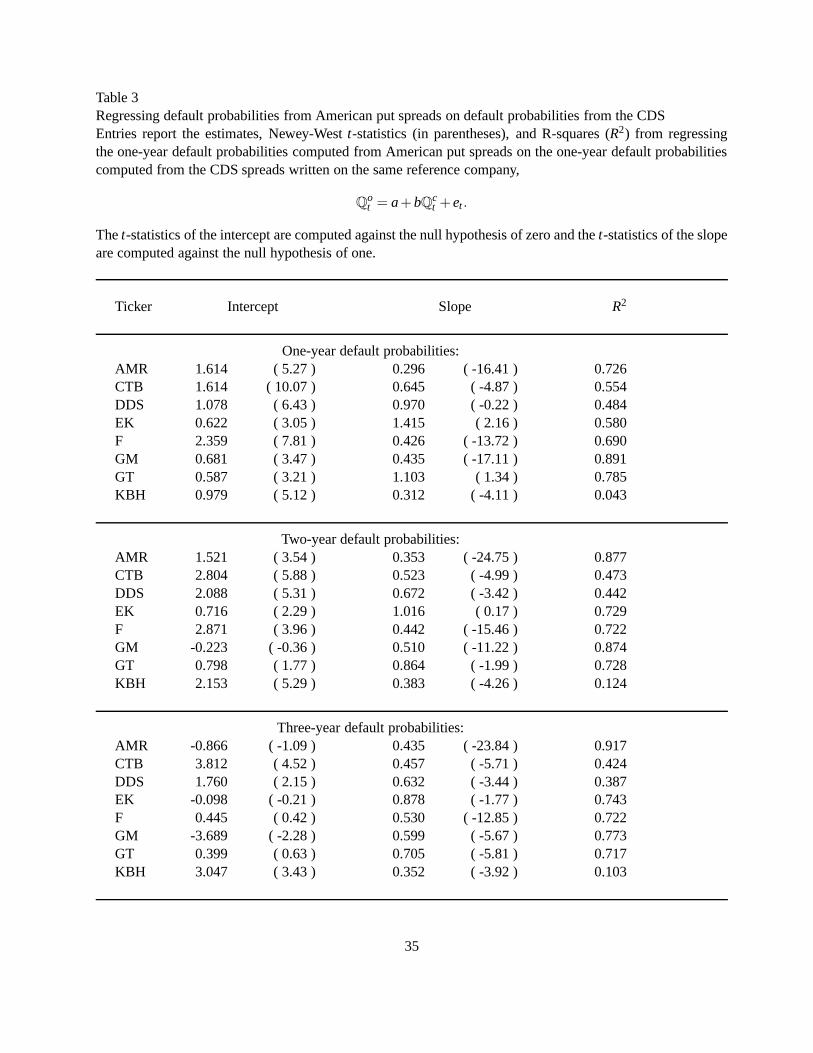
Table 3Regressing default probabilities from American put spreads on default probabilities from the CDSEntries report the estimates, Newey-Westt-statistics (in parentheses), and R-squares (R2) from regressingthe one-year default probabilities computed from Americanput spreads on the one-year default probabilitiescomputed from the CDS spreads written on the same reference company,

Qot = a+bQc

t +et .

Thet-statistics of the intercept are computed against the null hypothesis of zero and thet-statistics of the slopeare computed against the null hypothesis of one.

Ticker Intercept Slope R2

One-year default probabilities:AMR 1.614 ( 5.27 ) 0.296 ( -16.41 ) 0.726CTB 1.614 ( 10.07 ) 0.645 ( -4.87 ) 0.554DDS 1.078 ( 6.43 ) 0.970 ( -0.22 ) 0.484EK 0.622 ( 3.05 ) 1.415 ( 2.16 ) 0.580F 2.359 ( 7.81 ) 0.426 ( -13.72 ) 0.690GM 0.681 ( 3.47 ) 0.435 ( -17.11 ) 0.891GT 0.587 ( 3.21 ) 1.103 ( 1.34 ) 0.785KBH 0.979 ( 5.12 ) 0.312 ( -4.11 ) 0.043

Two-year default probabilities:AMR 1.521 ( 3.54 ) 0.353 ( -24.75 ) 0.877CTB 2.804 ( 5.88 ) 0.523 ( -4.99 ) 0.473DDS 2.088 ( 5.31 ) 0.672 ( -3.42 ) 0.442EK 0.716 ( 2.29 ) 1.016 ( 0.17 ) 0.729F 2.871 ( 3.96 ) 0.442 ( -15.46 ) 0.722GM -0.223 ( -0.36 ) 0.510 ( -11.22 ) 0.874GT 0.798 ( 1.77 ) 0.864 ( -1.99 ) 0.728KBH 2.153 ( 5.29 ) 0.383 ( -4.26 ) 0.124

Three-year default probabilities:AMR -0.866 ( -1.09 ) 0.435 ( -23.84 ) 0.917CTB 3.812 ( 4.52 ) 0.457 ( -5.71 ) 0.424DDS 1.760 ( 2.15 ) 0.632 ( -3.44 ) 0.387EK -0.098 ( -0.21 ) 0.878 ( -1.77 ) 0.743F 0.445 ( 0.42 ) 0.530 ( -12.85 ) 0.722GM -3.689 ( -2.28 ) 0.599 ( -5.67 ) 0.773GT 0.399 ( 0.63 ) 0.705 ( -5.81 ) 0.717KBH 3.047 ( 3.43 ) 0.352 ( -3.92 ) 0.103

35

Table 4Predicting future movements at daily horizon based on cross-market deviationsEntries report the estimates, Newey-Westt-statistics (in parentheses), and R-squares (R2) from the followingregressions,

∆Qot+∆t = ao +bo (Qo

t −cQct )+eo

t+∆t , ∆Qct+∆t = ac +bc (Qo

t −cQct )+ec

t+∆t,

where∆Qt+∆t denotes future changes over a one-day horizon, which are predicted by the deviations betweenthe estimates from the two markets.

Ticker ao bo R2 ac bc R2 c

One-year default probabilities:AMR 0.139 ( 2.46 ) -0.095 ( -2.38 ) 0.047 -0.060 ( -1.38 ) 0.022 (1.40 ) 0.003 0.304 ( 10.19 )CTB 0.381 ( 4.62 ) -0.229 ( -5.86 ) 0.108 -0.021 ( -0.93 ) 0.014 (1.38 ) 0.003 0.617 ( 11.95 )DDS 0.106 ( 2.57 ) -0.097 ( -3.08 ) 0.045 -0.007 ( -0.53 ) 0.008 (0.77 ) 0.003 0.931 ( 6.86 )EK 0.049 ( 2.93 ) -0.080 ( -4.27 ) 0.042 -0.003 ( -0.65 ) 0.005 ( 0.88 ) 0.001 1.441 ( 8.49 )F 0.342 ( 4.28 ) -0.140 ( -4.34 ) 0.069 0.036 ( 0.79 ) -0.013 ( -0.77 ) 0.001 0.413 ( 11.25 )GM 0.118 ( 2.87 ) -0.165 ( -5.51 ) 0.061 -0.075 ( -3.15 ) 0.109 ( 3.57 ) 0.041 0.431 ( 23.99 )GT 0.076 ( 3.58 ) -0.157 ( -6.20 ) 0.082 -0.007 ( -0.80 ) 0.011 ( 0.93 ) 0.002 1.136 ( 18.80 )KBH 0.058 ( 2.19 ) -0.060 ( -2.14 ) 0.030 0.001 ( 0.10 ) 0.002 ( 0.44 ) 0.000 0.353 ( 1.37 )

Two-year default probabilities:AMR 0.176 ( 3.04 ) -0.132 ( -2.43 ) 0.066 -0.074 ( -1.38 ) 0.012 (0.49 ) 0.001 0.353 ( 19.94 )CTB 0.606 ( 5.06 ) -0.207 ( -6.14 ) 0.099 -0.008 ( -0.27 ) 0.005 (0.68 ) 0.001 0.499 ( 9.85 )DDS 0.286 ( 4.18 ) -0.130 ( -4.37 ) 0.062 -0.014 ( -0.71 ) 0.008 (1.19 ) 0.003 0.641 ( 7.42 )EK 0.126 ( 3.16 ) -0.170 ( -4.13 ) 0.083 -0.004 ( -0.43 ) 0.007 ( 0.86 ) 0.001 1.009 ( 16.34 )F 0.464 ( 2.90 ) -0.154 ( -3.33 ) 0.078 0.012 ( 0.27 ) -0.001 ( -0.13 ) 0.000 0.434 ( 13.91 )GM -0.022 ( -0.44 ) -0.098 ( -4.11 ) 0.038 0.019 ( 0.40 ) 0.066 ( 2.19 ) 0.034 0.510 ( 18.41 )GT 0.047 ( 1.71 ) -0.099 ( -4.37 ) 0.050 -0.011 ( -0.52 ) 0.009 ( 0.86 ) 0.001 0.904 ( 12.11 )KBH 0.148 ( 4.02 ) -0.069 ( -3.96 ) 0.034 -0.002 ( -0.07 ) 0.004 (0.39 ) 0.000 0.390 ( 2.30 )

Three-year default probabilities:AMR -0.216 ( -1.87 ) -0.203 ( -3.57 ) 0.102 -0.016 ( -0.28 ) 0.042 ( 1.62 ) 0.008 0.435 ( 32.04 )CTB 0.764 ( 4.74 ) -0.191 ( -5.83 ) 0.092 -0.007 ( -0.17 ) 0.004 (0.58 ) 0.001 0.436 ( 8.65 )DDS 0.254 ( 3.47 ) -0.125 ( -4.15 ) 0.060 -0.009 ( -0.42 ) 0.007 (1.12 ) 0.003 0.596 ( 6.46 )EK -0.003 ( -0.08 ) -0.206 ( -4.86 ) 0.099 0.005 ( 0.36 ) 0.010 ( 1.52 ) 0.002 0.867 ( 18.68 )F 0.123 ( 1.23 ) -0.154 ( -3.62 ) 0.077 0.014 ( 0.34 ) 0.002 ( 0.22) 0.000 0.518 ( 14.10 )GM -0.234 ( -2.62 ) -0.069 ( -3.15 ) 0.030 0.082 ( 1.19 ) 0.022 ( 1.57 ) 0.011 0.588 ( 10.46 )GT -0.002 ( -0.05 ) -0.098 ( -4.24 ) 0.048 -0.011 ( -0.43 ) 0.009( 0.84 ) 0.001 0.731 ( 11.40 )KBH 0.250 ( 3.45 ) -0.083 ( -3.76 ) 0.042 0.002 ( 0.06 ) 0.003 ( 0.30 ) 0.000 0.363 ( 2.40 )

36

Table 5Predicting future movements at weekly horizon based on cross-market deviationsEntries report the estimates, Newey-Westt-statistics (in parentheses), and R-squares (R2) from the followingregressions,

∆Qot+∆t = ao +bo (Qo

t −cQct )+eo

t+∆t , ∆Qct+∆t = ac +bc (Qo

t −cQct )+ec

t+∆t,

where∆Qt+∆t denotes future changes over a one-week horizon, which are predicted by the deviations betweenthe estimates from the two markets.

Ticker ao bo R2 ac bc R2 c

One-year default probabilities:AMR 0.138 ( 1.48 ) -0.137 ( -1.88 ) 0.064 -0.216 ( -1.30 ) 0.062 (0.90 ) 0.007 0.325 ( 10.68 )CTB 0.672 ( 3.50 ) -0.398 ( -3.39 ) 0.141 -0.160 ( -1.98 ) 0.106 (2.79 ) 0.026 0.651 ( 14.10 )DDS 0.206 ( 2.69 ) -0.203 ( -3.48 ) 0.100 -0.046 ( -1.07 ) 0.048 (1.31 ) 0.020 1.033 ( 11.54 )EK 0.201 ( 3.25 ) -0.245 ( -3.82 ) 0.115 0.002 ( 0.07 ) 0.001 ( 0.04 ) 0.000 1.255 ( 12.11 )F 0.803 ( 4.14 ) -0.293 ( -4.33 ) 0.135 0.201 ( 1.03 ) -0.065 ( -1.01 ) 0.005 0.372 ( 12.05 )GM 0.113 ( 1.15 ) -0.219 ( -3.02 ) 0.053 -0.196 ( -1.68 ) 0.463 ( 3.98 ) 0.119 0.465 ( 34.92 )GT 0.137 ( 2.70 ) -0.324 ( -5.88 ) 0.149 -0.046 ( -1.16 ) 0.086 ( 1.50 ) 0.018 1.156 ( 24.62 )KBH 0.201 ( 3.04 ) -0.160 ( -3.26 ) 0.081 0.010 ( 0.29 ) 0.003 ( 0.17 ) 0.000 0.002 ( 0.01 )

Two-year default probabilities:AMR 0.223 ( 2.11 ) -0.253 ( -2.80 ) 0.126 -0.354 ( -1.71 ) 0.060 (0.68 ) 0.005 0.363 ( 23.63 )CTB 1.131 ( 3.80 ) -0.355 ( -3.43 ) 0.128 -0.041 ( -0.23 ) 0.022 (0.51 ) 0.002 0.492 ( 10.38 )DDS 0.584 ( 4.64 ) -0.262 ( -5.50 ) 0.130 -0.079 ( -1.06 ) 0.040 (1.55 ) 0.012 0.645 ( 10.63 )EK 0.347 ( 3.63 ) -0.428 ( -5.40 ) 0.198 0.003 ( 0.05 ) 0.015 ( 0.39 ) 0.001 1.002 ( 25.31 )F 0.982 ( 3.21 ) -0.295 ( -3.78 ) 0.142 0.006 ( 0.03 ) 0.018 ( 0.39) 0.001 0.421 ( 15.33 )GM -0.107 ( -0.75 ) -0.134 ( -2.10 ) 0.030 0.213 ( 0.93 ) 0.201 ( 2.19 ) 0.050 0.547 ( 21.50 )GT 0.042 ( 0.46 ) -0.253 ( -4.10 ) 0.122 -0.041 ( -0.44 ) 0.074 ( 1.34 ) 0.014 0.951 ( 18.65 )KBH 0.415 ( 4.08 ) -0.181 ( -4.37 ) 0.088 0.024 ( 0.19 ) 0.002 ( 0.04 ) 0.000 0.316 ( 2.61 )

Three-year default probabilities:AMR -0.517 ( -2.06 ) -0.348 ( -3.91 ) 0.152 -0.071 ( -0.23 ) 0.183 ( 1.76 ) 0.035 0.441 ( 36.73 )CTB 1.477 ( 3.96 ) -0.326 ( -3.56 ) 0.119 -0.022 ( -0.09 ) 0.016 (0.39 ) 0.001 0.417 ( 8.89 )DDS 0.527 ( 3.59 ) -0.245 ( -5.16 ) 0.121 -0.067 ( -0.78 ) 0.039 (1.47 ) 0.013 0.589 ( 8.88 )EK 0.022 ( 0.22 ) -0.516 ( -6.42 ) 0.240 0.026 ( 0.42 ) 0.031 ( 0.92 ) 0.003 0.868 ( 29.50 )F 0.352 ( 1.49 ) -0.287 ( -3.84 ) 0.133 0.071 ( 0.36 ) 0.037 ( 0.82) 0.003 0.508 ( 16.18 )GM -0.410 ( -1.62 ) -0.102 ( -2.15 ) 0.029 0.382 ( 1.26 ) 0.079 ( 1.41 ) 0.021 0.617 ( 12.09 )GT -0.080 ( -0.62 ) -0.238 ( -3.64 ) 0.111 -0.027 ( -0.23 ) 0.047( 0.93 ) 0.006 0.753 ( 16.25 )KBH 0.631 ( 4.15 ) -0.221 ( -4.70 ) 0.111 0.024 ( 0.14 ) 0.009 ( 0.22 ) 0.001 0.377 ( 3.73 )

37

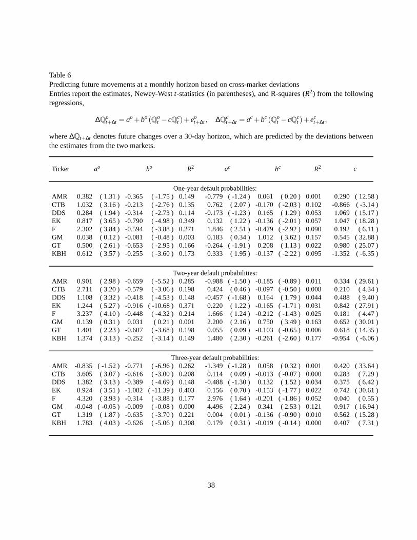
Table 6Predicting future movements at a monthly horizon based on cross-market deviationsEntries report the estimates, Newey-Westt-statistics (in parentheses), and R-squares (R2) from the followingregressions,

∆Qot+∆t = ao +bo (Qo

t −cQct )+eo

t+∆t , ∆Qct+∆t = ac +bc (Qo

t −cQct )+ec

t+∆t,

where∆Qt+∆t denotes future changes over a 30-day horizon, which are predicted by the deviations betweenthe estimates from the two markets.

Ticker ao bo R2 ac bc R2 c

One-year default probabilities:AMR 0.382 ( 1.31 ) -0.365 ( -1.75 ) 0.149 -0.779 ( -1.24 ) 0.061 (0.20 ) 0.001 0.290 ( 12.58 )CTB 1.032 ( 3.16 ) -0.213 ( -2.76 ) 0.135 0.762 ( 2.07 ) -0.170 ( -2.03 ) 0.102 -0.866 ( -3.14 )DDS 0.284 ( 1.94 ) -0.314 ( -2.73 ) 0.114 -0.173 ( -1.23 ) 0.165 (1.29 ) 0.053 1.069 ( 15.17 )EK 0.817 ( 3.65 ) -0.790 ( -4.98 ) 0.349 0.132 ( 1.22 ) -0.136 ( -2.01 ) 0.057 1.047 ( 18.28 )F 2.302 ( 3.84 ) -0.594 ( -3.88 ) 0.271 1.846 ( 2.51 ) -0.479 ( -2.92 ) 0.090 0.192 ( 6.11 )GM 0.038 ( 0.12 ) -0.081 ( -0.48 ) 0.003 0.183 ( 0.34 ) 1.012 ( 3.62 ) 0.157 0.545 ( 32.88 )GT 0.500 ( 2.61 ) -0.653 ( -2.95 ) 0.166 -0.264 ( -1.91 ) 0.208 ( 1.13 ) 0.022 0.980 ( 25.07 )KBH 0.612 ( 3.57 ) -0.255 ( -3.60 ) 0.173 0.333 ( 1.95 ) -0.137 ( -2.22 ) 0.095 -1.352 ( -6.35 )

Two-year default probabilities:AMR 0.901 ( 2.98 ) -0.659 ( -5.52 ) 0.285 -0.988 ( -1.50 ) -0.185( -0.89 ) 0.011 0.334 ( 29.61 )CTB 2.711 ( 3.20 ) -0.579 ( -3.06 ) 0.198 0.424 ( 0.46 ) -0.097 ( -0.50 ) 0.008 0.210 ( 4.34 )DDS 1.108 ( 3.32 ) -0.418 ( -4.53 ) 0.148 -0.457 ( -1.68 ) 0.164 (1.79 ) 0.044 0.488 ( 9.40 )EK 1.244 ( 5.27 ) -0.916 ( -10.68 ) 0.371 0.220 ( 1.22 ) -0.165 ( -1.71 ) 0.031 0.842 ( 27.91 )F 3.237 ( 4.10 ) -0.448 ( -4.32 ) 0.214 1.666 ( 1.24 ) -0.212 ( -1.43 ) 0.025 0.181 ( 4.47 )GM 0.139 ( 0.31 ) 0.031 ( 0.21 ) 0.001 2.200 ( 2.16 ) 0.750 ( 3.49 )0.163 0.652 ( 30.01 )GT 1.401 ( 2.23 ) -0.607 ( -3.68 ) 0.198 0.055 ( 0.09 ) -0.103 ( -0.65 ) 0.006 0.618 ( 14.35 )KBH 1.374 ( 3.13 ) -0.252 ( -3.14 ) 0.149 1.480 ( 2.30 ) -0.261 ( -2.60 ) 0.177 -0.954 ( -6.06 )

Three-year default probabilities:AMR -0.835 ( -1.52 ) -0.771 ( -6.96 ) 0.262 -1.349 ( -1.28 ) 0.058 ( 0.32 ) 0.001 0.420 ( 33.64 )CTB 3.605 ( 3.07 ) -0.616 ( -3.00 ) 0.208 0.114 ( 0.09 ) -0.013 ( -0.07 ) 0.000 0.283 ( 7.29 )DDS 1.382 ( 3.13 ) -0.389 ( -4.69 ) 0.148 -0.488 ( -1.30 ) 0.132 (1.52 ) 0.034 0.375 ( 6.42 )EK 0.924 ( 3.51 ) -1.002 ( -11.39 ) 0.403 0.156 ( 0.70 ) -0.153 ( -1.77 ) 0.022 0.742 ( 30.61 )F 4.320 ( 3.93 ) -0.314 ( -3.88 ) 0.177 2.976 ( 1.64 ) -0.201 ( -1.86 ) 0.052 0.040 ( 0.55 )GM -0.048 ( -0.05 ) -0.009 ( -0.08 ) 0.000 4.496 ( 2.24 ) 0.341 ( 2.53 ) 0.121 0.917 ( 16.94 )GT 1.319 ( 1.87 ) -0.635 ( -3.70 ) 0.221 0.004 ( 0.01 ) -0.136 ( -0.90 ) 0.010 0.562 ( 15.28 )KBH 1.783 ( 4.03 ) -0.626 ( -5.06 ) 0.308 0.179 ( 0.31 ) -0.019 ( -0.14 ) 0.000 0.407 ( 7.31 )

38

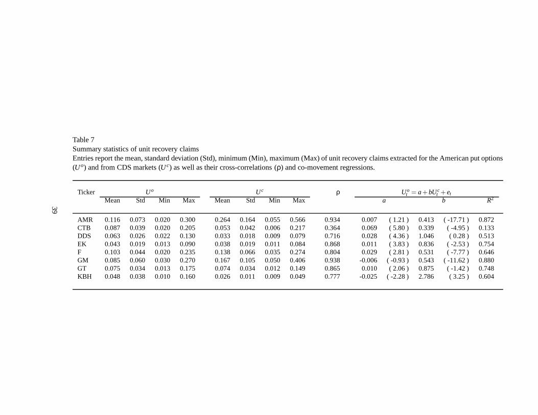
Table 7Summary statistics of unit recovery claimsEntries report the mean, standard deviation (Std), minimum(Min), maximum (Max) of unit recovery claims extracted for the American put options(Uo) and from CDS markets (Uc) as well as their cross-correlations (ρ) and co-movement regressions.

Ticker Uo Uc ρ Uot = a+bUc

t +et

Mean Std Min Max Mean Std Min Max a b R2

AMR 0.116 0.073 0.020 0.300 0.264 0.164 0.055 0.566 0.934 0.007 ( 1.21 ) 0.413 ( -17.71 ) 0.872CTB 0.087 0.039 0.020 0.205 0.053 0.042 0.006 0.217 0.364 0.069 ( 5.80 ) 0.339 ( -4.95 ) 0.133DDS 0.063 0.026 0.022 0.130 0.033 0.018 0.009 0.079 0.716 0.028 ( 4.36 ) 1.046 ( 0.28 ) 0.513EK 0.043 0.019 0.013 0.090 0.038 0.019 0.011 0.084 0.868 0.011 ( 3.83 ) 0.836 ( -2.53 ) 0.754F 0.103 0.044 0.020 0.235 0.138 0.066 0.035 0.274 0.804 0.029( 2.81 ) 0.531 ( -7.77 ) 0.646GM 0.085 0.060 0.030 0.270 0.167 0.105 0.050 0.406 0.938 -0.006 ( -0.93 ) 0.543 ( -11.62 ) 0.880GT 0.075 0.034 0.013 0.175 0.074 0.034 0.012 0.149 0.865 0.010 ( 2.06 ) 0.875 ( -1.42 ) 0.748KBH 0.048 0.038 0.010 0.160 0.026 0.011 0.009 0.049 0.777 -0.025 ( -2.28 ) 2.786 ( 3.25 ) 0.604

39

Table 8Predicting future movements on unit recovery claims based on cross-market deviationsEntries report the estimates, Newey-Westt-statistics (in parentheses), and R-squares (R2) from the following regression that predicts futuremovements in the unit recovery claim synthesized by American puts (Uo) based on its deviations from the CDS market valuations,

∆Uot+∆t = α+ β(Uo

t −bUct )+et ,

where forecasting horizons (∆t) are at one, seven, and 30 days and the cointegrating coefficientsb are obtained from the level regressions inTable 7.

Ticker One days Seven days 30 daysα β R2 α β R2 α β R2

AMR -0.000 ( -0.08 ) -0.070 ( -2.75 ) 0.034 -0.001 ( -0.99 ) -0.175 ( -2.48 ) 0.079 -0.006 ( -1.20 ) -0.598 ( -3.76 ) 0.241CTB 0.001 ( 1.51 ) -0.015 ( -1.44 ) 0.005 0.005 ( 1.33 ) -0.056 ( -1.20 ) 0.015 0.012 ( 1.17 ) -0.144 ( -1.07 ) 0.029DDS 0.000 ( 1.81 ) -0.022 ( -2.66 ) 0.012 0.002 ( 1.53 ) -0.088 ( -2.55 ) 0.052 0.004 ( 1.26 ) -0.290 ( -3.10 ) 0.159EK 0.001 ( 4.84 ) -0.093 ( -4.36 ) 0.053 0.003 ( 5.12 ) -0.297 ( -6.03 ) 0.172 0.011 ( 4.46 ) -0.969 ( -9.93 ) 0.422F 0.002 ( 3.23 ) -0.077 ( -2.89 ) 0.050 0.006 ( 2.74 ) -0.201 ( -2.63 ) 0.111 0.017 ( 2.72 ) -0.571 ( -3.34 ) 0.227GM -0.001 ( -1.60 ) -0.122 ( -3.42 ) 0.051 -0.001 ( -0.71 ) -0.162 ( -2.65 ) 0.040 -0.002 ( -0.41 ) -0.226 ( -1.03 ) 0.021GT 0.000 ( 1.00 ) -0.063 ( -3.66 ) 0.032 0.001 ( 0.53 ) -0.184 ( -2.50 ) 0.077 0.001 ( 0.22 ) -0.599 ( -2.33 ) 0.192KBH -0.000 ( -1.14 ) -0.008 ( -1.29 ) 0.002 -0.000 ( -0.32 ) -0.004 ( -0.10 ) 0.000 -0.001 ( -0.29 ) 0.043 ( 0.53 ) 0.007

40

Table 9Default probabilities estimated from a structural modelEntries report the mean, standard deviation (Std), minimum(Min), maximum (Max), daily autocorrelation(Auto) of companies’ one-year default probabilities (in percentage points) estimated from Merton (1974)’sstructural model. The computations uses the stock price as the per share equity value and net debt per share asthe per share debt face value, and computes the firm value assuming equality between the market and the facevalue of the debt. To compute firm volatility, the left panel uses one-standard deviation out-of-money stockoption implied volatility as input whereas the right panel uses at-the-money stock option implied volatility asinput.

Ticker From out-of-money option From at-the-money optionMean Std Min Max Auto ρ Mean Std Min Max Auto ρ

One-year default probabilities:AMR 9.802 8.058 0.311 33.791 0.994 0.797 3.308 3.259 0.045 13.566 0.989 0.775CTB 0.112 0.367 0.000 2.730 0.940 0.770 0.019 0.080 0.000 0.795 0.888 0.699DDS 0.033 0.042 0.000 0.198 0.957 0.651 0.002 0.006 0.000 0.048 0.884 0.188EK 0.001 0.004 0.000 0.036 0.939 0.677 0.000 0.000 0.000 0.002 0.902 0.619F 3.235 2.588 0.003 14.763 0.976 0.854 0.860 0.857 0.000 5.742 0.966 0.778GM 7.731 9.970 0.017 41.668 0.993 0.972 2.574 4.270 0.000 20.658 0.989 0.925GT 0.848 0.791 0.003 4.222 0.977 0.812 0.113 0.140 0.000 0.929 0.968 0.713KBH 0.071 0.112 0.000 0.588 0.980 0.019 0.010 0.022 0.000 0.131 0.966 -0.037

Two-year default probabilities:AMR 28.704 18.392 2.478 67.296 0.996 0.943 12.353 9.776 0.752 36.588 0.994 0.910CTB 1.066 2.273 0.000 13.112 0.975 0.818 0.279 0.729 0.000 5.214 0.963 0.802DDS 0.812 0.703 0.001 2.784 0.983 0.687 0.131 0.137 0.000 0.605 0.971 0.599EK 0.135 0.267 0.000 1.618 0.985 0.801 0.011 0.029 0.000 0.200 0.971 0.697F 15.745 8.577 0.329 38.120 0.987 0.863 6.611 4.397 0.045 19.536 0.986 0.847GM 22.611 20.341 1.151 66.385 0.991 0.986 9.616 11.711 0.11242.363 0.993 0.970GT 6.058 3.477 0.447 19.845 0.983 0.879 1.587 1.156 0.058 7.282 0.978 0.821KBH 1.335 1.122 0.009 5.095 0.989 0.340 0.300 0.381 0.000 1.680 0.988 0.203

Three-year default probabilities:AMR 41.376 21.973 6.651 81.109 0.996 0.959 21.152 14.182 2.723 52.169 0.994 0.933CTB 2.702 4.681 0.000 23.995 0.981 0.823 0.882 1.813 0.000 10.697 0.977 0.828DDS 2.702 1.916 0.031 7.508 0.985 0.655 0.677 0.577 0.001 2.352 0.980 0.632EK 0.652 0.992 0.000 5.285 0.988 0.825 0.087 0.183 0.000 1.070 0.982 0.732F 26.971 12.132 1.438 55.102 0.986 0.861 13.424 7.491 0.348 32.729 0.986 0.836GM 28.763 18.319 3.612 69.028 0.969 0.860 16.605 16.903 0.658 59.480 0.994 0.943GT 12.838 6.038 1.975 32.946 0.981 0.861 4.457 2.563 0.387 15.092 0.980 0.802KBH 4.081 2.614 0.136 12.174 0.985 0.549 1.220 1.121 0.008 4.571 0.989 0.447

41

0 2 4 6 8 10 12 140.2

0.3

0.4

0.5

0.6

0.7

0.8

0.9

1

Mean default probability, %

Cros

s−co

rrela

tion

Time to maturity: 1 year

0 5 10 15 20 25 30

0.4

0.5

0.6

0.7

0.8

0.9

1

Mean default probability, %

Cros

s−co

rrela

tion

Time to maturity: 2 years

5 10 15 20 25 30 35 40

0.4

0.5

0.6

0.7

0.8

0.9

1

Mean default probability, %

Cros

s−co

rrela

tion

Time to maturity: 3 years

Fig. 1. Cross correlations as function of mean default probabilities.The graphs show the relation between the mean default probability level (computed from the CDS market)and the cross-correlation estimates between the default probabilities computed from the two markets. Thedots are data points. The lines are local-linear smoothing fits. Each panel represents one maturity.

42

0 2 4 6 8 10 12 14−7

−6

−5

−4

−3

−2

−1

0

1

2

Mean default probability, %

Mea

n bi

as, Q

o −Qc , %

Time to maturity: 1 year

0 5 10 15 20 25 30−16

−14

−12

−10

−8

−6

−4

−2

0

2

Mean default probability, %

Mea

n bi

as, Q

o −Qc , %

Time to maturity: 2 years

5 10 15 20 25 30 35 40−25

−20

−15

−10

−5

0

5

Mean default probability, %

Mea

n bi

as, Q

o −Qc , %

Time to maturity: 3 years

Fig. 2. Mean biases in default probabilities.The dots in each panel represent the mean difference betweenthe default probabilities estimated from theoptions market and that from the CDS market. The solid lines are local-linear smoothing fits. Each panelrepresents one maturity.

43

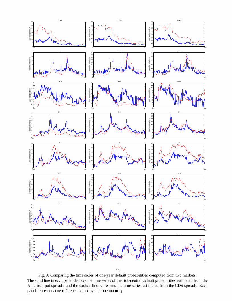
05 070

5

10

15

20

25

30

35

1−ye

ar de

fault p

robab

ility, %

AMR

05 070

10

20

30

40

50

60

2−ye

ar de

fault p

robab

ility, %

AMR

05 070

10

20

30

40

50

60

70

80

3−ye

ar de

fault p

robab

ility, %

AMR

05 070

2

4

6

8

10

12

1−ye

ar de

fault p

robab

ility, %

CTB

05 070

2

4

6

8

10

12

14

16

18

20

2−ye

ar de

fault p

robab

ility, %

CTB

05 070

5

10

15

20

25

30

3−ye

ar de

fault p

robab

ility, %

CTB

05 070

0.5

1

1.5

2

2.5

3

3.5

4

4.5

1−ye

ar de

fault p

robab

ility, %

DDS

05 071

2

3

4

5

6

7

8

2−ye

ar de

fault p

robab

ility, %

DDS

05 072

3

4

5

6

7

8

9

10

11

12

3−ye

ar de

fault p

robab

ility, %

DDS

05 070

1

2

3

4

5

6

7

1−ye

ar de

fault p

robab

ility, %

EK

05 070

2

4

6

8

10

12

2−ye

ar de

fault p

robab

ility, %

EK

05 070

2

4

6

8

10

12

14

16

18

3−ye

ar de

fault p

robab

ility, %

EK

05 070

2

4

6

8

10

12

14

16

1−ye

ar de

fault p

robab

ility, %

F

05 070

5

10

15

20

25

30

2−ye

ar de

fault p

robab

ility, %

F

05 070

5

10

15

20

25

30

35

40

3−ye

ar de

fault p

robab

ility, %

F

05 070

5

10

15

20

25

1−ye

ar de

fault p

robab

ility, %

GM

05 070

5

10

15

20

25

30

35

40

45

2−ye

ar de

fault p

robab

ility, %

GM

05 070

10

20

30

40

50

60

3−ye

ar de

fault p

robab

ility, %

GM

05 070

1

2

3

4

5

6

7

8

9

1−ye

ar de

fault p

robab

ility, %

GT

05 070

2

4

6

8

10

12

14

2−ye

ar de

fault p

robab

ility, %

GT

05 070

5

10

15

20

25

3−ye

ar de

fault p

robab

ility, %

GT

05 070

0.5

1

1.5

2

2.5

3

3.5

4

1−ye

ar de

fault p

robab

ility, %

KBH

05 071

2

3

4

5

6

7

2−ye

ar de

fault p

robab

ility, %

KBH

05 070

2

4

6

8

10

12

14

3−ye

ar de

fault p

robab

ility, %

KBH

Fig. 3. Comparing the time series of one-year default probabilities computed from two markets.The solid line in each panel denotes the time series of the risk-neutral default probabilities estimated from theAmerican put spreads, and the dashed line represents the time series estimated from the CDS spreads. Eachpanel represents one reference company and one maturity.

44

05 070

0.05

0.1

0.15

0.2

0.25

0.3

0.35

Unit

reco

very

cla

im

AMR

05 070

0.05

0.1

0.15

0.2

0.25

Unit

reco

very

cla

im

CTB

05 070

0.02

0.04

0.06

0.08

0.1

0.12

0.14

Unit

reco

very

cla

im

DDS

05 070

0.01

0.02

0.03

0.04

0.05

0.06

0.07

0.08

0.09

0.1

Unit

reco

very

cla

im

EK

05 070

0.05

0.1

0.15

0.2

0.25

Unit

reco

very

cla

im

F

05 070

0.05

0.1

0.15

0.2

0.25

0.3

0.35

Unit

reco

very

cla

im

GM

05 070

0.02

0.04

0.06

0.08

0.1

0.12

0.14

0.16

0.18

0.2

Unit

reco

very

cla

im

GT

05 07−0.02

0

0.02

0.04

0.06

0.08

0.1

0.12

0.14

0.16

0.18

Unit

reco

very

cla

im

KBH

Fig. 4. Tracing the unit recovery values.The solid lines are the market values of the unit recovery claim synthesized from American put options. Thedashed lines are the estimated values from the CDS quotes based on constant interest rate and default arrivalrate assumption and linear interpolation on the CDS quotes.

45

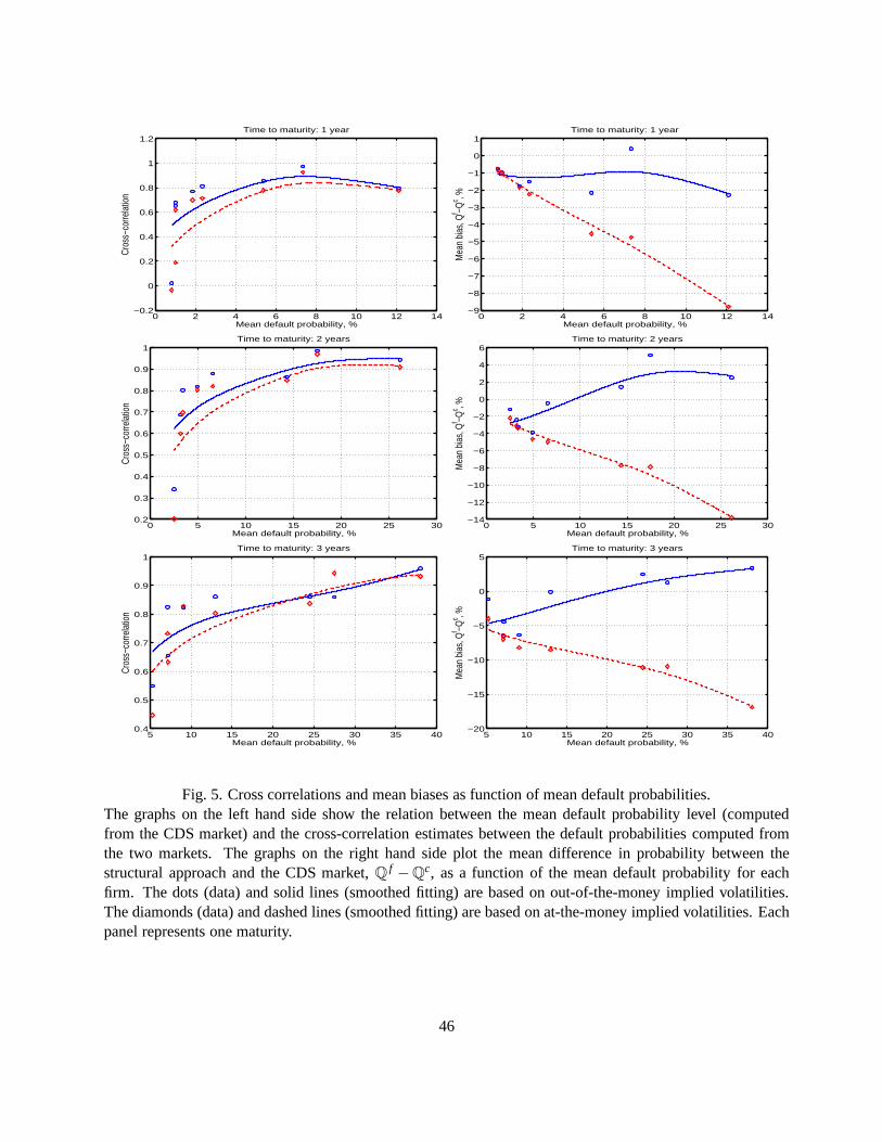
0 2 4 6 8 10 12 14−0.2

0

0.2

0.4

0.6

0.8

1

1.2

Mean default probability, %

Cros

s−co

rrela

tion

Time to maturity: 1 year

0 2 4 6 8 10 12 14−9

−8

−7

−6

−5

−4

−3

−2

−1

0

1

Mean default probability, %

Mea

n bi

as, Q

f −Qc , %

Time to maturity: 1 year

0 5 10 15 20 25 300.2

0.3

0.4

0.5

0.6

0.7

0.8

0.9

1

Mean default probability, %

Cros

s−co

rrela

tion

Time to maturity: 2 years

0 5 10 15 20 25 30−14

−12

−10

−8

−6

−4

−2

0

2

4

6

Mean default probability, %

Mea

n bi

as, Q

f −Qc , %

Time to maturity: 2 years

5 10 15 20 25 30 35 400.4

0.5

0.6

0.7

0.8

0.9

1

Mean default probability, %

Cros

s−co

rrela

tion

Time to maturity: 3 years

5 10 15 20 25 30 35 40−20

−15

−10

−5

0

5

Mean default probability, %

Mea

n bi

as, Q

f −Qc , %

Time to maturity: 3 years

Fig. 5. Cross correlations and mean biases as function of mean default probabilities.The graphs on the left hand side show the relation between themean default probability level (computedfrom the CDS market) and the cross-correlation estimates between the default probabilities computed fromthe two markets. The graphs on the right hand side plot the mean difference in probability between thestructural approach and the CDS market,Q f −Qc, as a function of the mean default probability for eachfirm. The dots (data) and solid lines (smoothed fitting) are based on out-of-the-money implied volatilities.The diamonds (data) and dashed lines (smoothed fitting) are based on at-the-money implied volatilities. Eachpanel represents one maturity.

46